symmetry and visual hallucinations
TRANSCRIPT
Symmetry and Visual Hallucinations
Martin GolubitskyMathematical Biosciences Institute
Ohio State University
Paul Bressloff Jack CowanUtah Chicago
Peter Thomas Matthew WienerCase Western Neuropsychology, NIH
Lie June Shiau Andrew TörökHouston Clear Lake Houston
Klüver: We wish to stress . . . one point, namely, that under
diverse conditions the visual system responds in terms of a
limited number of form constants.
– p. 1/43

Why Study Patterns I
1. Science behind patterns
– p. 2/43

Columnar Joints on Staffa near Mull
– p. 3/43

Columns along Snake River
– p. 4/43
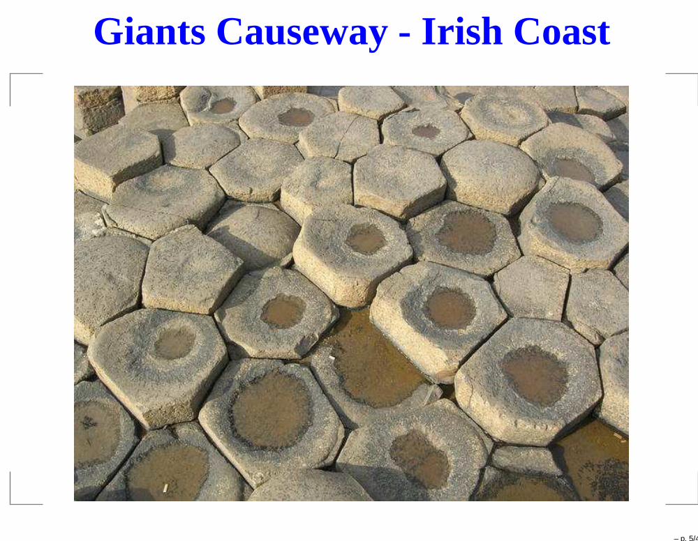
Giants Causeway - Irish Coast
– p. 5/43
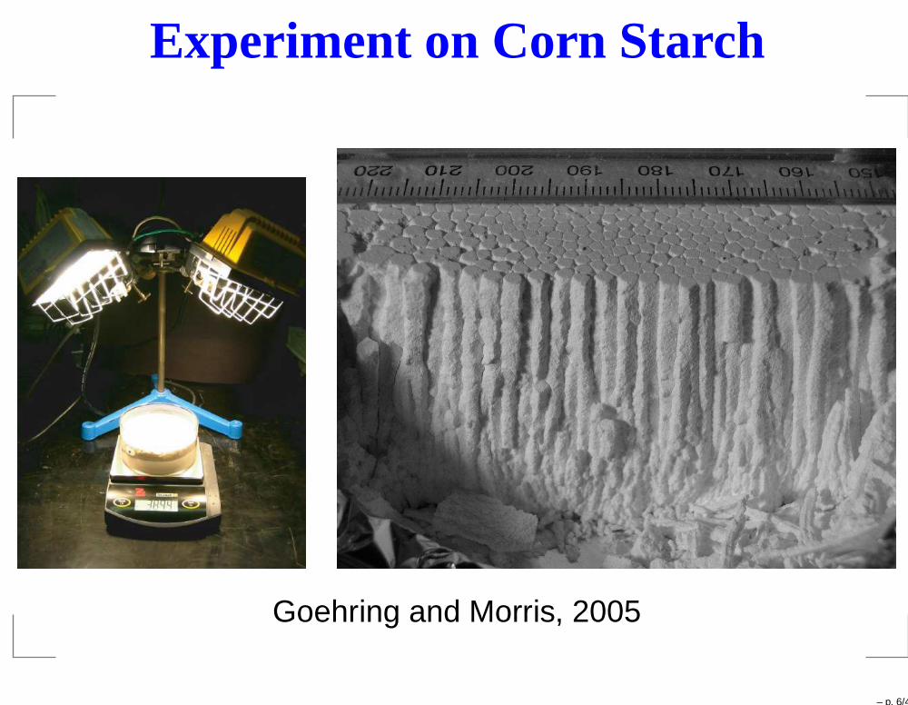
Experiment on Corn Starch
Goehring and Morris, 2005
– p. 6/43

Why Study Patterns II
1. Science behind patterns
2. Change in patterns provide tests for models
– p. 7/43
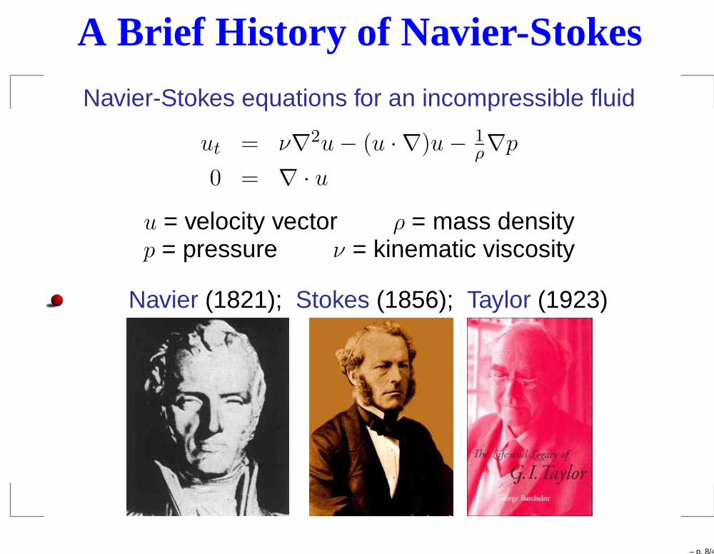
A Brief History of Navier-Stokes
Navier-Stokes equations for an incompressible fluid
ut = ν∇2u − (u · ∇)u − 1ρ∇p
0 = ∇ · u
u = velocity vector ρ = mass densityp = pressure ν = kinematic viscosity
Navier (1821); Stokes (1856); Taylor (1923)
– p. 8/43
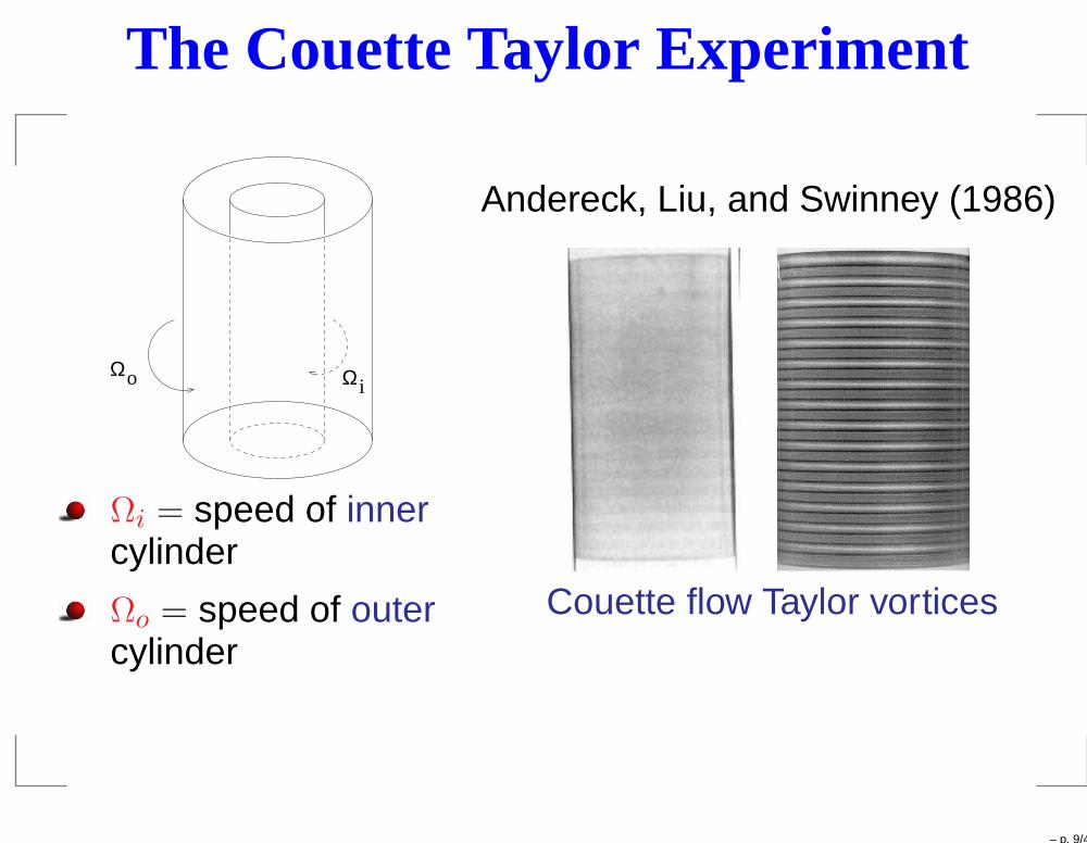
The Couette Taylor Experiment
Ω Ωo i
Ωi = speed of innercylinder
Ωo = speed of outercylinder
Andereck, Liu, and Swinney (1986)
Couette flow Taylor vortices
– p. 9/43
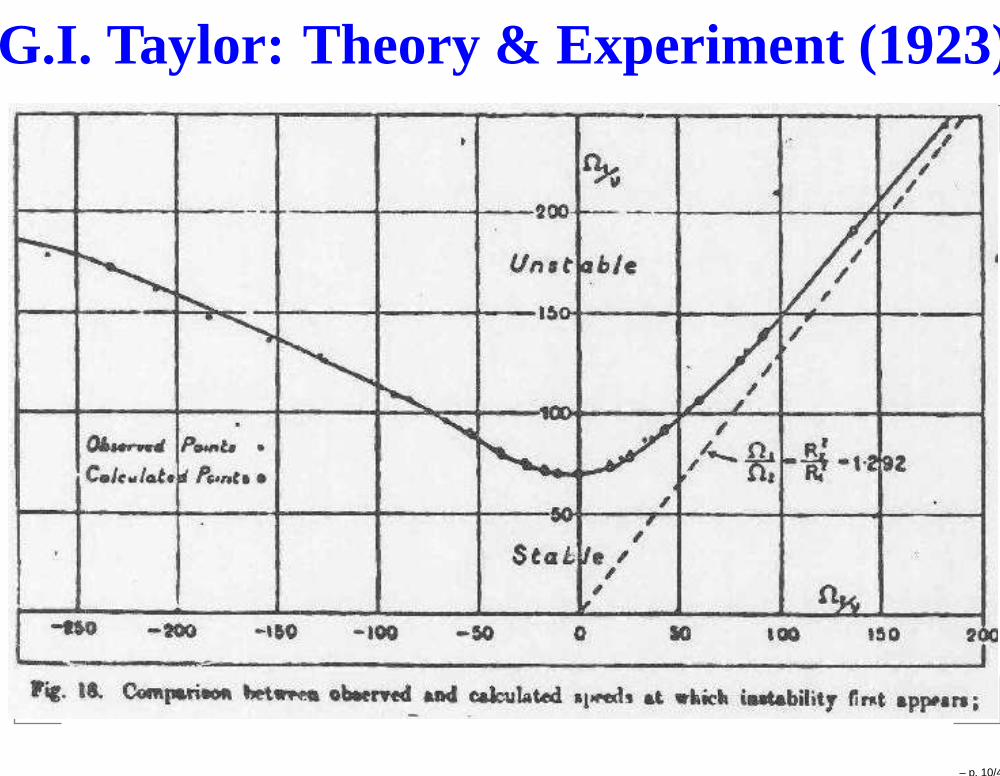
G.I. Taylor: Theory & Experiment (1923)
– p. 10/43
Why Study Patterns III
1. Science behind patterns
2. Change in patterns provide tests for models
3. Model independence
Mathematics provides menu of patterns
– p. 11/43
Planar Symmetry-Breaking
Euclidean symmetry: translations, rotations, reflections
Symmetry-breaking from translation invariant state inplanar systems with Euclidean symmetry leads to
Stripes:States invariant under translation in one direction
Spots:
States centered at lattice points
– p. 12/43

Sand Dunes in Namibian Desert
– p. 13/43
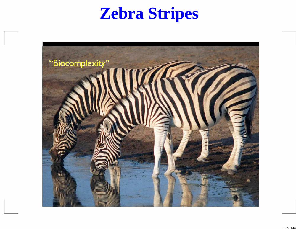
Zebra Stripes
– p. 14/43

Mud Plains
– p. 15/43
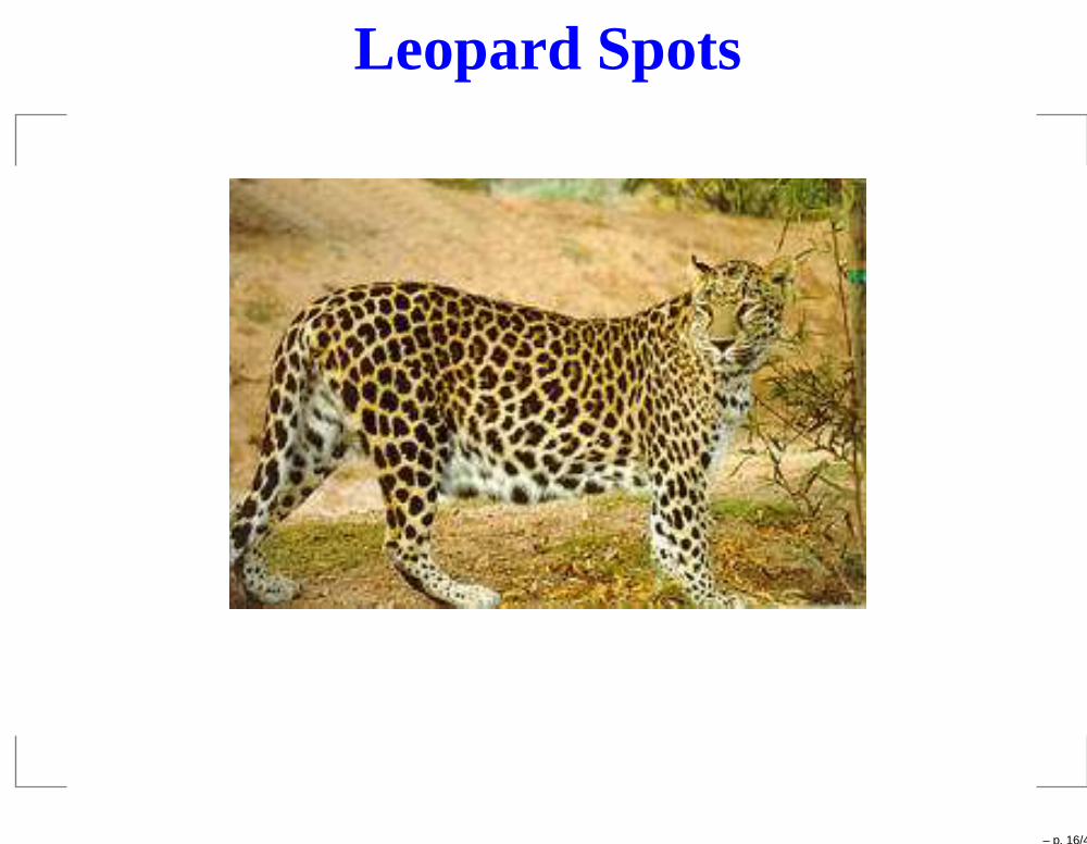
Leopard Spots
– p. 16/43
Outline
1. Geometric Visual Hallucinations
2. Structure of Visual Cortex
Hubel and Wiesel hypercolumns; local and lateralconnections; isotropy versus anisotropy
3. Pattern Formation in V1
Symmetry; Three models
4. Interpretation of Patterns in Retinal Coordinates
– p. 17/43
Visual Hallucinations
Drug uniformly forces activation of cortical cells
Leads to spontaneous pattern formation on cortex
Map from V1 to retina;translates pattern on cortex to visual image
– p. 18/43
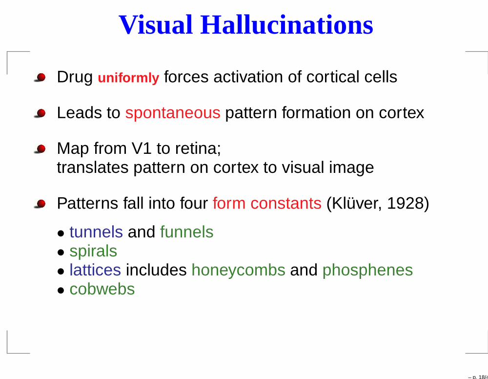
Visual Hallucinations
Drug uniformly forces activation of cortical cells
Leads to spontaneous pattern formation on cortex
Map from V1 to retina;translates pattern on cortex to visual image
Patterns fall into four form constants (Klüver, 1928)
• tunnels and funnels• spirals• lattices includes honeycombs and phosphenes• cobwebs
– p. 18/43
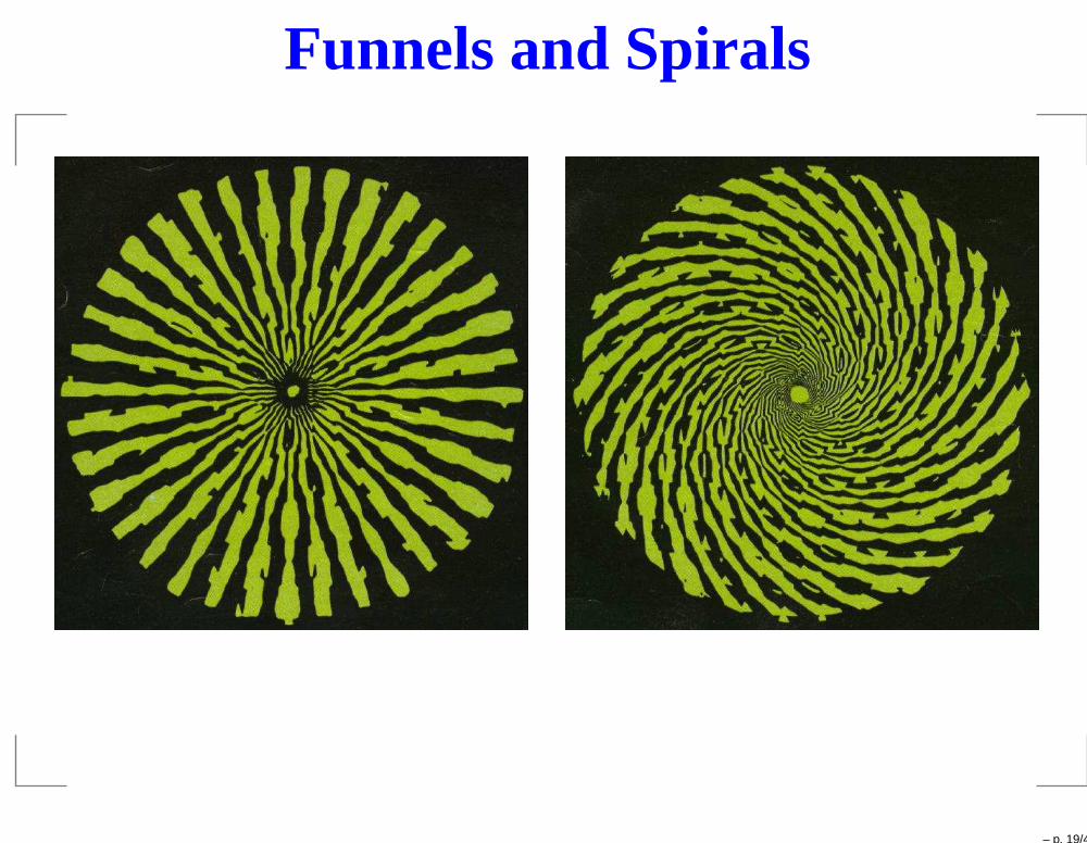
Funnels and Spirals
– p. 19/43

Lattices: Honeycombs & Phosphenes
– p. 20/43
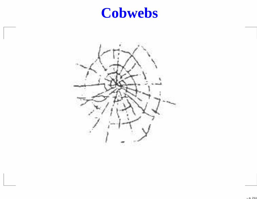
Cobwebs
– p. 21/43
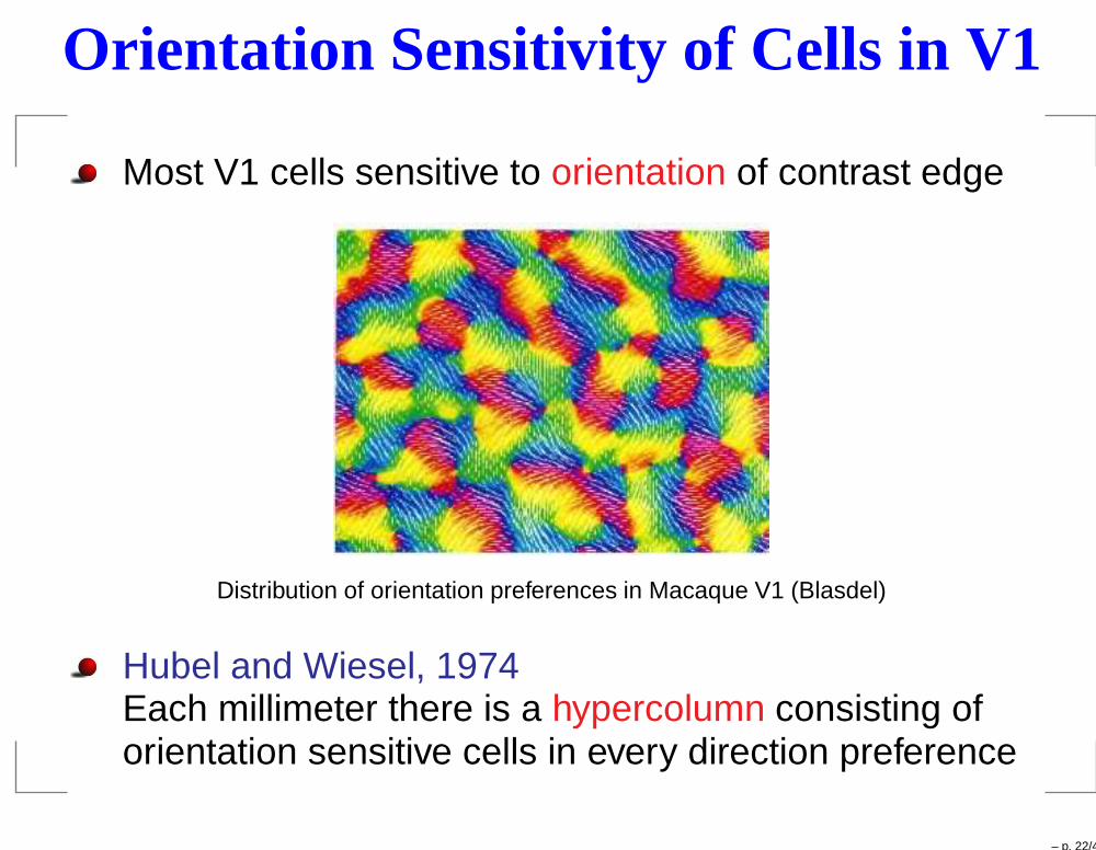
Orientation Sensitivity of Cells in V1
Most V1 cells sensitive to orientation of contrast edge
Distribution of orientation preferences in Macaque V1 (Blasdel)
Hubel and Wiesel, 1974Each millimeter there is a hypercolumn consisting oforientation sensitive cells in every direction preference
– p. 22/43
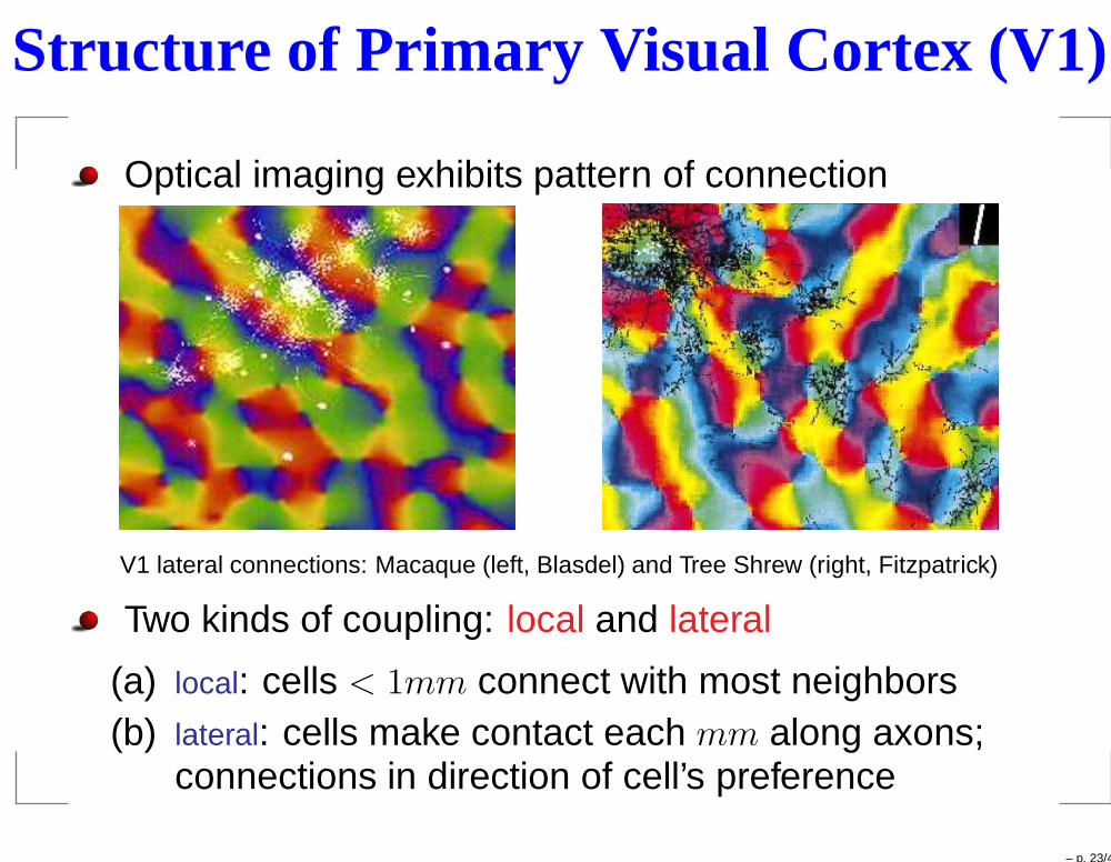
Structure of Primary Visual Cortex (V1)
Optical imaging exhibits pattern of connection
V1 lateral connections: Macaque (left, Blasdel) and Tree Shrew (right, Fitzpatrick)
Two kinds of coupling: local and lateral
(a) local: cells < 1mm connect with most neighbors(b) lateral: cells make contact each mm along axons;
connections in direction of cell’s preference
– p. 23/43
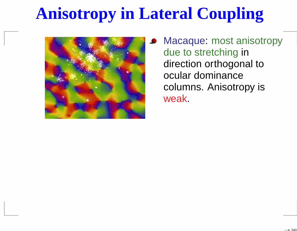
Anisotropy in Lateral Coupling
Macaque: most anisotropydue to stretching indirection orthogonal toocular dominancecolumns. Anisotropy isweak.
– p. 24/43
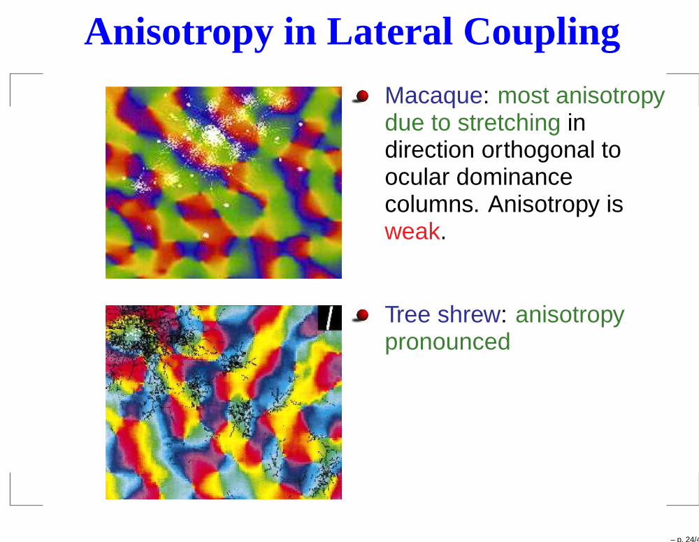
Anisotropy in Lateral Coupling
Macaque: most anisotropydue to stretching indirection orthogonal toocular dominancecolumns. Anisotropy isweak.
Tree shrew: anisotropypronounced
– p. 24/43
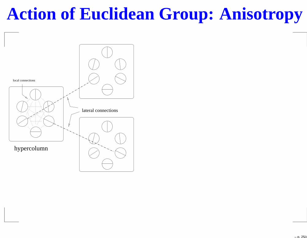
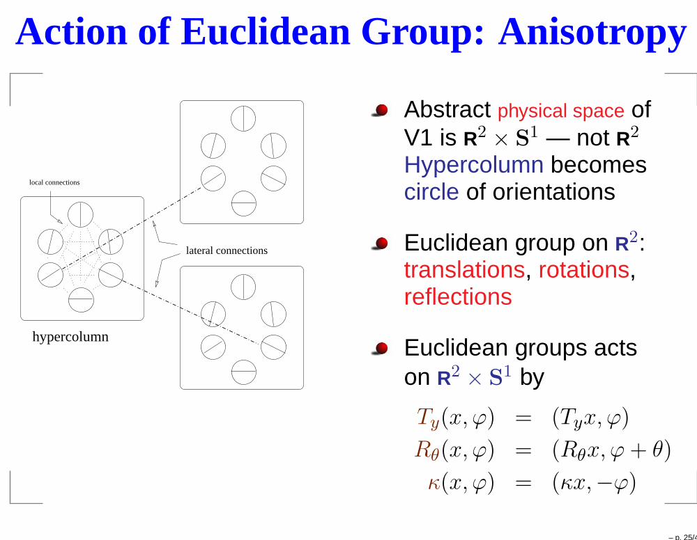
Action of Euclidean Group: Anisotropy
hypercolumn
lateral connections
local connections
– p. 25/43
Action of Euclidean Group: Anisotropy
hypercolumn
lateral connections
local connections
Abstract physical space ofV1 is R2 × S
1 — not R2
Hypercolumn becomescircle of orientations
Euclidean group on R2:translations, rotations,reflections
Euclidean groups actson R2 × S
1 by
Ty(x, ϕ) = (Tyx, ϕ)
Rθ(x, ϕ) = (Rθx, ϕ + θ)
κ(x, ϕ) = (κx,−ϕ)
– p. 25/43
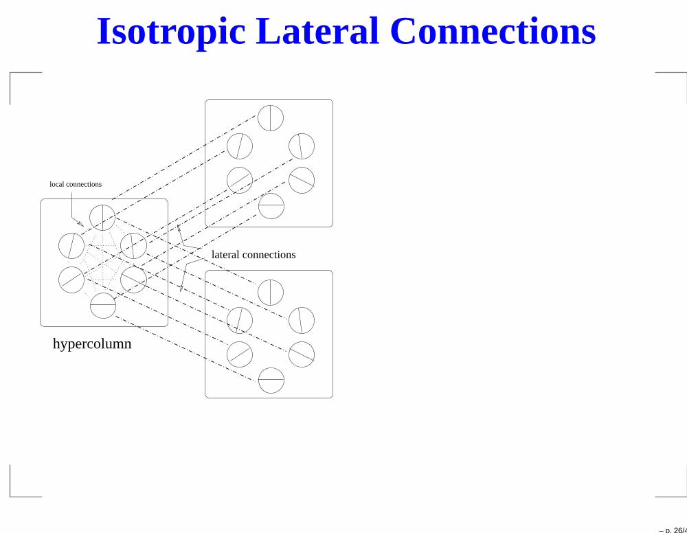
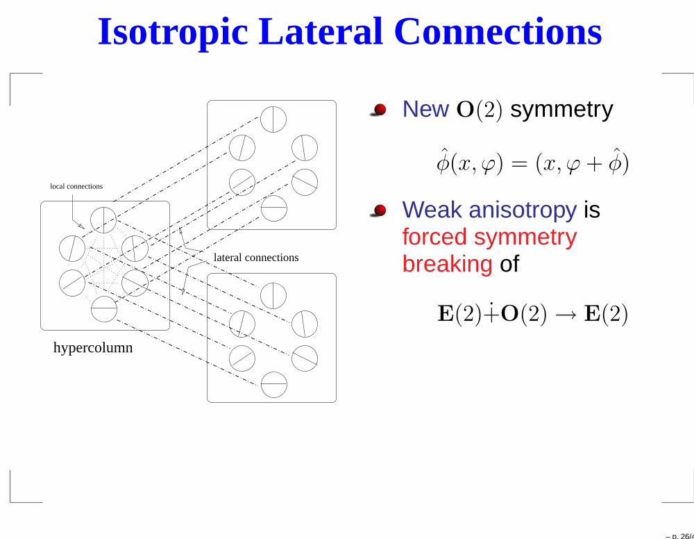
Isotropic Lateral Connections
hypercolumn
lateral connections
local connections
– p. 26/43
Isotropic Lateral Connections
hypercolumn
lateral connections
local connections
New O(2) symmetry
φ(x, ϕ) = (x, ϕ + φ)
Weak anisotropy isforced symmetrybreaking of
E(2)+O(2) → E(2)
– p. 26/43
Three Models
E(2) acting on R2 (Ermentrout-Cowan)neurons located at each point xActivity variable: a(x) = voltage potential of neuronPattern given by threshold a(x) > v0
– p. 27/43
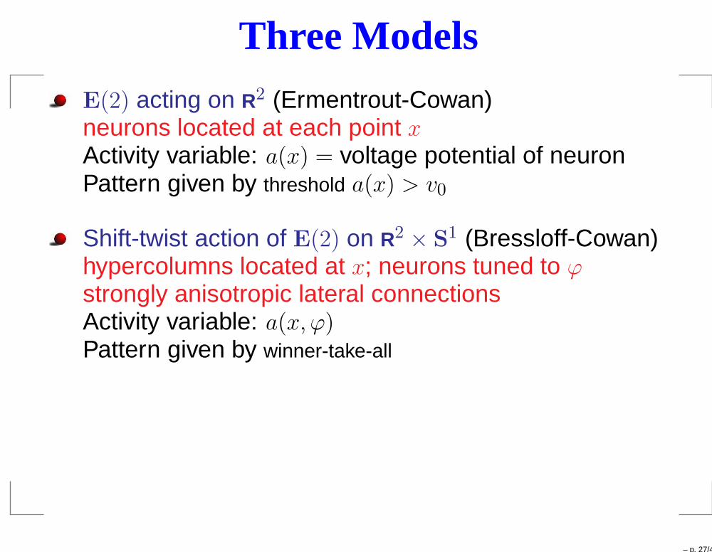
Three Models
E(2) acting on R2 (Ermentrout-Cowan)neurons located at each point xActivity variable: a(x) = voltage potential of neuronPattern given by threshold a(x) > v0
Shift-twist action of E(2) on R2 × S1 (Bressloff-Cowan)
hypercolumns located at x; neurons tuned to ϕstrongly anisotropic lateral connectionsActivity variable: a(x, ϕ)Pattern given by winner-take-all
Symmetry breaking: E(2)+O(2) → E(2)weakly anisotropic lateral couplingActivity variable: a(x, ϕ)Pattern given by winner-take-all
– p. 27/43
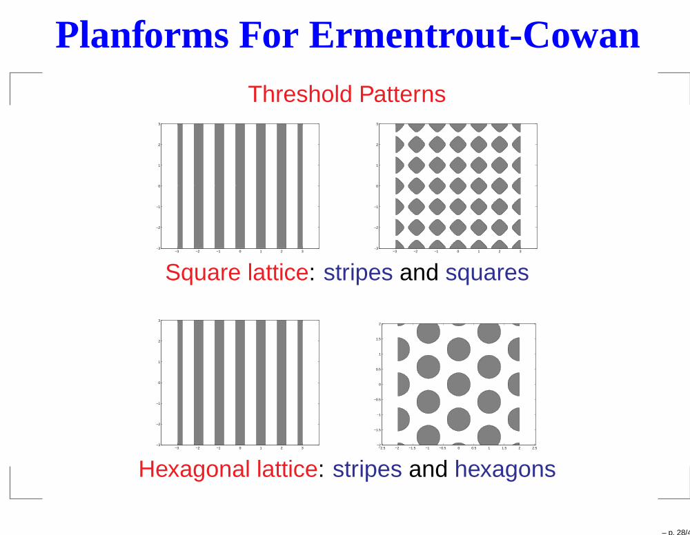
Planforms For Ermentrout-CowanThreshold Patterns
−3 −2 −1 0 1 2 3−3
−2
−1
0
1
2
3
−3 −2 −1 0 1 2 3−3
−2
−1
0
1
2
3
Square lattice: stripes and squares
−3 −2 −1 0 1 2 3−3
−2
−1
0
1
2
3
−2.5 −2 −1.5 −1 −0.5 0 0.5 1 1.5 2 2.5−2
−1.5
−1
−0.5
0
0.5
1
1.5
2
Hexagonal lattice: stripes and hexagons
– p. 28/43

Winner-Take-All Strategy
Creation of Line Fields
Given: Activity a(x, ϕ) of neuron in hypercolumn at x
sensitive to direction ϕ
Assumption: Most active neuron in hypercolumnsuppresses other neurons in hypercolumn
Consequence: For all x find direction ϕx where activityis maximum
Planform: Line segment at each x oriented at angle ϕx
– p. 29/43
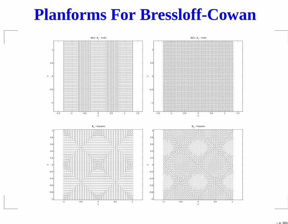
Planforms For Bressloff-Cowan
−1.5 −1 −0.5 0 0.5 1 1.5
−1
−0.5
0
0.5
1
x
y
O(2)⊕ Z2 − Erolls
−1.5 −1 −0.5 0 0.5 1 1.5
−1
−0.5
0
0.5
1
x
y
O(2)⊕ Z4 − Orolls
−1 −0.5 0 0.5 1−1
−0.8
−0.6
−0.4
−0.2
0
0.2
0.4
0.6
0.8
1
x
y
D4 − Esquares
−1 −0.5 0 0.5 1−1
−0.8
−0.6
−0.4
−0.2
0
0.2
0.4
0.6
0.8
1
x
y
D4 − Osquares
– p. 30/43

Cortex to Retina
Neurons on cortex are uniformly distributed
Neurons in retina fall off by 1/r2 from fovea
Unique angle preserving map takes uniform densitysquare to 1/r2 density disk: complex exponential
Straight lines on cortex 7→circles, logarithmic spirals, and rays in retina
– p. 31/43
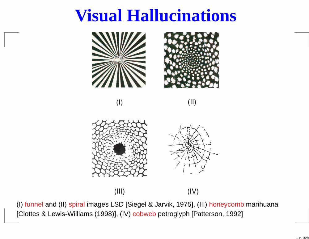
Visual Hallucinations
(I) (II)
(III) (IV)(I) funnel and (II) spiral images LSD [Siegel & Jarvik, 1975], (III) honeycomb marihuana[Clottes & Lewis-Williams (1998)], (IV) cobweb petroglyph [Patterson, 1992]
– p. 32/43
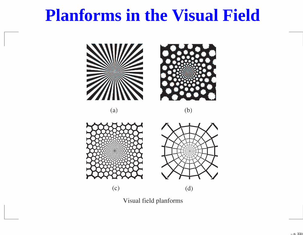
Planforms in the Visual Field
(a) (b)
(c) (d)Visual field planforms
– p. 33/43
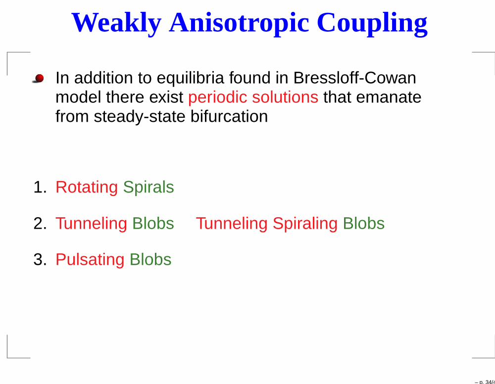
Weakly Anisotropic Coupling
In addition to equilibria found in Bressloff-Cowanmodel there exist periodic solutions that emanatefrom steady-state bifurcation
1. Rotating Spirals
2. Tunneling Blobs Tunneling Spiraling Blobs
3. Pulsating Blobs
– p. 34/43
Pattern Formation Outline
1. Bifurcation Theory with Symmetry
Equivariant Branching LemmaModel independent analysis
2. Translations lead to plane waves
3. Planforms: Computation of eigenfunctions
– p. 35/43
Primer on Steady-State Bifurcation
Solve x = f(x, λ) = 0 where f : Rn × R → Rn
Local theory: Assume f(0, 0) = 0 & find solns near (0, 0)
If L = (dxf)0,0 nonsingular, IFT implies unique soln x(λ)
– p. 36/43
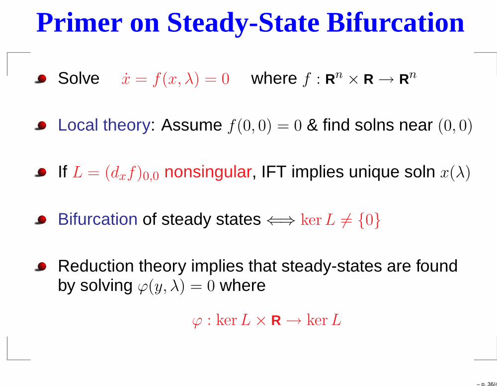
Primer on Steady-State Bifurcation
Solve x = f(x, λ) = 0 where f : Rn × R → Rn
Local theory: Assume f(0, 0) = 0 & find solns near (0, 0)
If L = (dxf)0,0 nonsingular, IFT implies unique soln x(λ)
Bifurcation of steady states ⇐⇒ ker L 6= 0
Reduction theory implies that steady-states are foundby solving ϕ(y, λ) = 0 where
ϕ : ker L × R → ker L
– p. 36/43

Equivariant Steady-State Bifurcation
Let γ : Rn → Rn be linear
γ is a symmetry iff γ(soln)=soln iff f(γx, λ) = γf(x, λ)
Chain rule =⇒ Lγ = γL =⇒ ker L is γ-invariant
Theorem: Fix symmetry group Γ. Genericallyker L is an absolutely irreducible representation of Γ
Reduction implies that there is a unique steady-statebifurcation theory for each absolutely irreducible rep
– p. 37/43
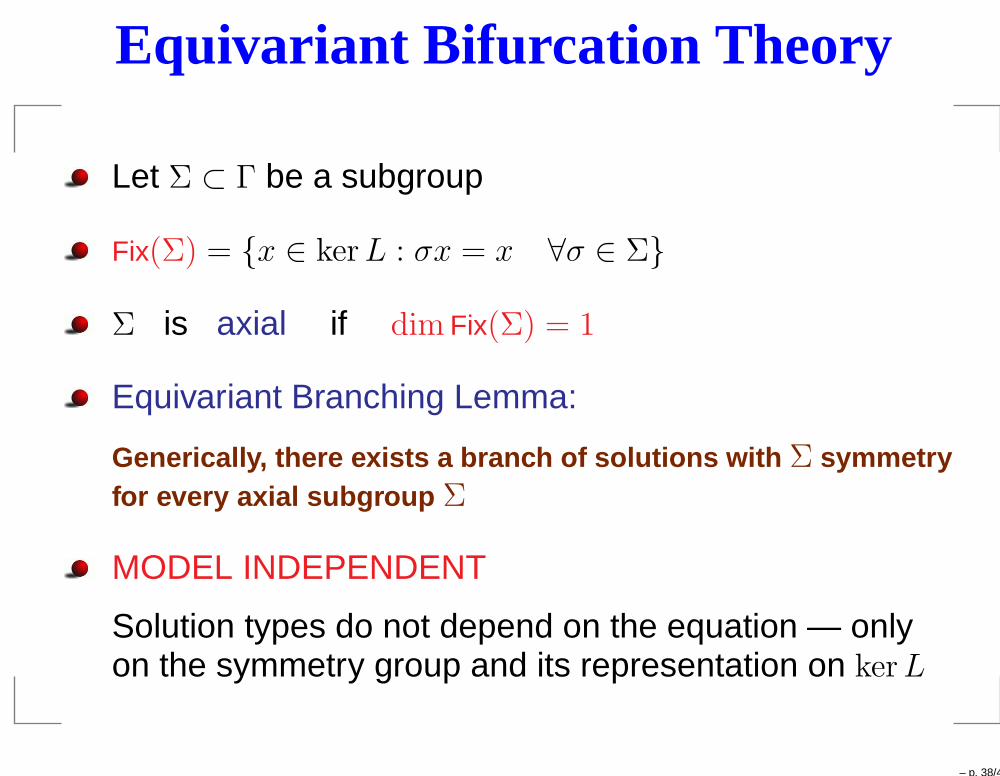
Equivariant Bifurcation Theory
Let Σ ⊂ Γ be a subgroup
Fix(Σ) = x ∈ ker L : σx = x ∀σ ∈ Σ
Σ is axial if dim Fix(Σ) = 1
Equivariant Branching Lemma:
Generically, there exists a branch of solutions with Σ symmetryfor every axial subgroup Σ
MODEL INDEPENDENT
Solution types do not depend on the equation — onlyon the symmetry group and its representation on ker L
– p. 38/43
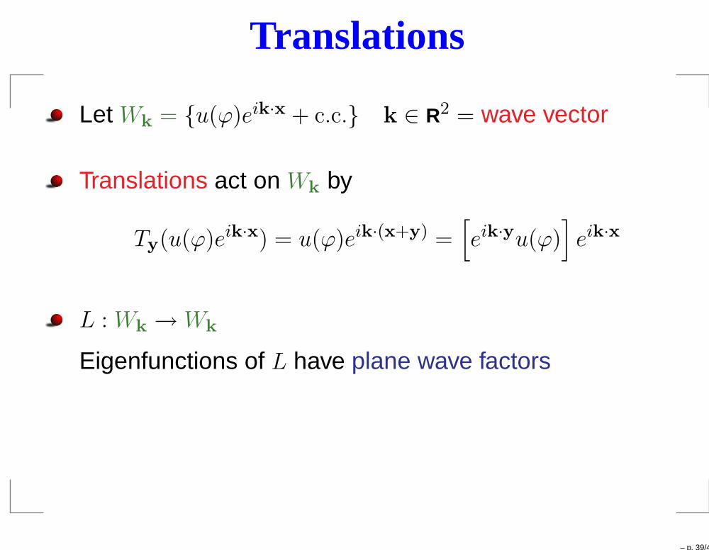
Translations
Let Wk = u(ϕ)eik·x + c.c. k ∈ R2 = wave vector
Translations act on Wk by
Ty(u(ϕ)eik·x) = u(ϕ)eik·(x+y) =[
eik·yu(ϕ)]
eik·x
L : Wk → Wk
Eigenfunctions of L have plane wave factors
– p. 39/43
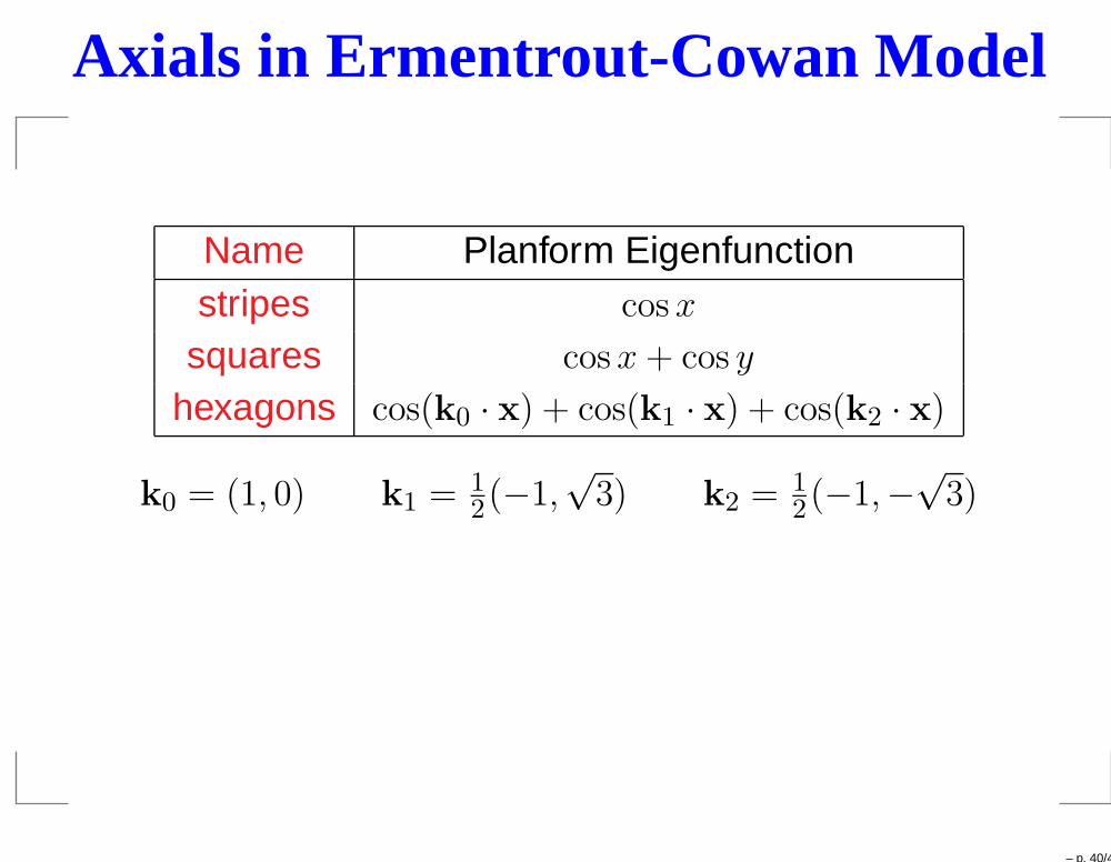
Axials in Ermentrout-Cowan Model
Name Planform Eigenfunctionstripes cos x
squares cos x + cos y
hexagons cos(k0 · x) + cos(k1 · x) + cos(k2 · x)
k0 = (1, 0) k1 = 12(−1,
√3) k2 = 1
2(−1,−√
3)
– p. 40/43
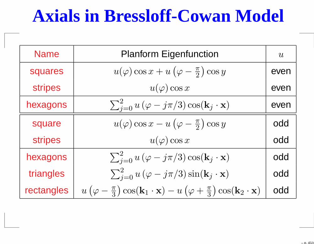
Axials in Bressloff-Cowan Model
Name Planform Eigenfunction u
squares u(ϕ) cos x + u(
ϕ − π2
)
cos y even
stripes u(ϕ) cos x even
hexagons∑
2
j=0u (ϕ − jπ/3) cos(kj · x) even
square u(ϕ) cos x − u(
ϕ − π2
)
cos y odd
stripes u(ϕ) cos x odd
hexagons∑
2
j=0u (ϕ − jπ/3) cos(kj · x) odd
triangles∑
2
j=0u (ϕ − jπ/3) sin(kj · x) odd
rectangles u(
ϕ − π3
)
cos(k1 · x) − u(
ϕ + π3
)
cos(k2 · x) odd
– p. 41/43
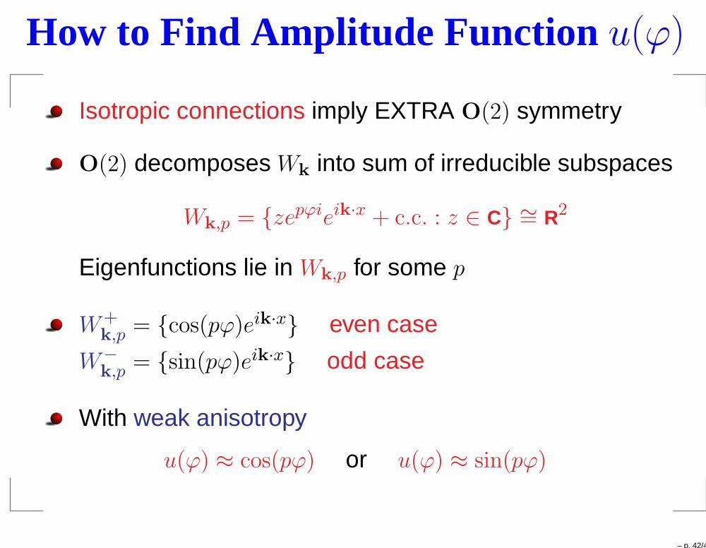
How to Find Amplitude Function u(ϕ)
Isotropic connections imply EXTRA O(2) symmetry
O(2) decomposes Wk into sum of irreducible subspaces
Wk,p = zepϕieik·x + c.c. : z ∈ C ∼= R2
Eigenfunctions lie in Wk,p for some p
W+k,p = cos(pϕ)eik·x even case
W−
k,p = sin(pϕ)eik·x odd case
With weak anisotropy
u(ϕ) ≈ cos(pϕ) or u(ϕ) ≈ sin(pϕ)
– p. 42/43
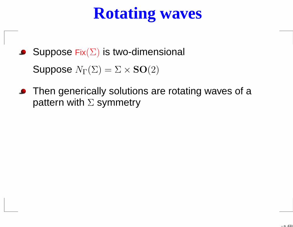
Rotating waves
Suppose Fix(Σ) is two-dimensional
Suppose NΓ(Σ) = Σ × SO(2)
Then generically solutions are rotating waves of apattern with Σ symmetry
– p. 43/43