Symbolic Computation forNonlinear Wave Resonances

E. Kartashova, C. Raab, Ch. Feurer,G. Mayrhofer, W. Schreiner

Research Institute for Symbolic Computation (RISC)Johannes Kepler University Linz

Altenbergerstr. 69, A-4040 Linz, Austria

6th December 2007

1

Contents

1 Introduction 3

2 Mathematical Background 5

3 Equations for Wave Amplitudes 73.1 Method Description . . . . . . . . . . . . . . . . . . . . . . . . 73.2 The Implementation . . . . . . . . . . . . . . . . . . . . . . . 8

3.2.1 Perturbation Equations, General Form . . . . . . . . . 103.2.2 Perturbation Equations, Given Linear Mode . . . . . . 113.2.3 Time and Scale Averaging . . . . . . . . . . . . . . . . 11

3.3 Obstacles . . . . . . . . . . . . . . . . . . . . . . . . . . . . . 133.4 Results . . . . . . . . . . . . . . . . . . . . . . . . . . . . . . . 14

3.4.1 Atmospheric Planetary Waves . . . . . . . . . . . . . . 143.4.2 Ocean Planetary Waves . . . . . . . . . . . . . . . . . 16

4 Resonance Conditions 164.1 Method Description . . . . . . . . . . . . . . . . . . . . . . . . 174.2 The Implementation . . . . . . . . . . . . . . . . . . . . . . . 18

4.2.1 List of Indexes . . . . . . . . . . . . . . . . . . . . . . 184.2.2 Weight Equation . . . . . . . . . . . . . . . . . . . . . 194.2.3 Linear Condition . . . . . . . . . . . . . . . . . . . . . 204.2.4 Scale Coefficients . . . . . . . . . . . . . . . . . . . . . 20

4.3 Results . . . . . . . . . . . . . . . . . . . . . . . . . . . . . . . 21

5 Structure of the Solution Set 215.1 Method Description . . . . . . . . . . . . . . . . . . . . . . . . 215.2 Implementation . . . . . . . . . . . . . . . . . . . . . . . . . . 235.3 Results . . . . . . . . . . . . . . . . . . . . . . . . . . . . . . . 255.4 Important Remark . . . . . . . . . . . . . . . . . . . . . . . . 28

6 A Web Interface to the Software 286.1 The Interface . . . . . . . . . . . . . . . . . . . . . . . . . . . 296.2 The Implementation . . . . . . . . . . . . . . . . . . . . . . . 316.3 Extensions . . . . . . . . . . . . . . . . . . . . . . . . . . . . . 35

7 Discussion 35

2

1 Introduction

Resonance is a common thread which runs through almost every branch ofphysics, without resonance we wouldn’t have radio, television, music, etc.Resonance causes an object to oscillate, sometimes the oscillation is easy tosee (vibration in a guitar string), but sometimes this is impossible withoutmeasuring instruments (electrons in an electrical circuit). A well-known ex-ample with Tacoma Narrows Bridge (at the time it opened for traffic in 1940,it was the third longest suspension bridge in the world) shows how disastrousresonances can be: on the morning of November 7, 1940, the four month oldTacoma Narrows Bridge began to oscillate dangerously up and down, toreitself apart and collapsed. Though designed for winds of 120 mph, a windof only 42 mph caused it to collapse. The experts did agree that somehowthe wind caused the bridge to resonate, and nowadays, wind tunnel testingof bridge designs is mandatory.

Another famous example are the experiments of Tesla who studied in 1898experimentally vibrations of an iron column and noticed that at certain fre-quencies specific pieces of equipment in the room would start to jiggle. Play-ing with the frequency he was able to move the jiggle to another part of theroom. Completely fascinated with these findings, he forgot that the columnran downward into the foundation of the building, and the vibrations werebeing transmitted all over Manhattan. The experiments had started sort of asmall earthquake in his neighborhood with smashed windows, swayed build-ings, and panicky people in the streets. For Tesla, the first hint of troublecame when the walls and floor began to heave [1]. He stopped the experimentas soon as he saw police rushing through the door.

The difference between resonances in a human made system and in somenatural phenomena is very simple. We can change the form of a bridgeand stop the experiment by switching off electricity but we can not changethe direction of the wind, the form of the Earth atmosphere or the sizes ofan ocean. What we can try to do is to predict drastic behavior of a realphysical system by computing its resonances. While linear resonances indifferent physical systems are comparatively well studied, to compute char-acteristics of nonlinear resonances and to predict their properties is quite anontrivial problem, even in the one-dimensional case. Thus, the notoriousFermi-Pasta-Ulam numerical experiments with a nonlinear 1D-string (car-ried out more then 50 years ago) are still not fully understood [2]. On theother hand, nonlinear wave resonances in continuous 2D-media like ocean,space, atmosphere, plasma, etc. are well studied in the frame of wave tur-bulence theory [4] and provide a sound basis for qualitative and sometimes

3

also quantitative analysis of corresponding physical systems. The notion ofnonlinear wave interactions is crucial in the wave turbulence theory [3]. Ex-cluding resonances allows to describe a nonlinear wave system statistically, bywave kinetic equations and power-law energy spectra of turbulence [5], andto observe this behavior in numerical experiments [6]. Direct computationswith Euler equations (modified for gravity water waves, [7]) show that theexistence of resonances in a wave system yield some additional effects whichare not covered by the statistical description. The role of resonances in theevolution of water wave turbulent systems has been studied profoundly bya great number of researchers. One of the most important conclusions (forgravity water waves) made recently in [8] is the following: ”The four-waveresonant interactions control the evolution of the spectrum at every instantof time, whereas non-resonant interactions do not make any significant con-tribution even in a short-term evolution.”

The behavior of a resonant wave system can be briefly described [9] as follows:1) not all waves take part in resonant interactions, 2) resonantly interactingwaves form a few independent small wave clusters, such that there is noenergy flow between these clusters, 3) including some small but non-zeroresonance width into consideration does not destroy the clusters. A modelof laminated wave turbulence [10] allows to describe statistical and resonantregimes simultaneously while methods to compute resonances numericallyare presented in [12] (idea) and in [13] (implementation). Our main purposehere is to study the possibilities of a symbolic implementation of these generalalgorithms using the computer algebra system Mathematica.

The implemented software can be executed with local installations of Math-ematica and the corresponding method libraries; however, we have also de-veloped a Web interface that allows to run the methods from any computerin the Internet via a conventional Web browser. The implementation strat-egy is simple and based on generally available technologies; it can serve as ablueprint for other mathematical software with similar features.

We take as our principal example the barotropic vorticity equation in arectangular domain with zero boundary conditions which describes oceanicplanetary waves, and show how : (a) to compute interaction coefficients ofcorresponding dynamical systems, (b) to solve resonant conditions, (c) toconstruct the topological structure of the solution set, and (d) to use thesoftware via a Web interface over the Internet. A short discussion concludesthe paper.

4

2 Mathematical Background

Wave turbulence takes place in physical systems with nonlinear dispersivewaves thatare described by evolutionary dispersive NPDEs. The role of theevolutionary dispersive NPDEs in the theoretical physics is so importantthat the notion of dispersion is used for a physical classification of PDEs intodispersive and non-dispersive. The well-known mathematical classification ofPDEs into elliptic, parabolic and hyperbolic equations is based on the formof equations and can be applied to the second order PDEs on an arbitrarynumber of variables. On the other hand, the physical classification is basedon the form of solutions and can be applied to PDEs of arbitrary order andarbitrary number of variables. In order to construct the physical classificationof PDEs, two preliminary steps are to be made: 1) to divide all variables intotwo groups - time- and space-like variables (t and x correspondingly); and 2)to check that the linear part of the PDE under consideration has a wave-likesolution in the form of Fourier harmonic

ψ(x, t) = A exp i[kx− ωt]

with amplitude A, wave-number k and wave frequency ω. The direct substi-tution of this solution into the linear PDE shows then that ω is an explicitfunction on k, for instance:

ψt + ψx + ψxxx = 0 ⇒ ω(k) = k − 5k3.

If ω as a function on k is real-valued and such that d2ω/dk2 6= 0, it iscalled a dispersion function and the corresponding PDE is called evolutionarydispersive PDE. If the dimension of the space variable x is more that1, i.e. ~x = (x1, ..., xp), ~k is called the wave-vector and the dispersion

function ω = ω(~k) depends on the coordinates of the wave-vector. Thisclassification is not complementary to a standard mathematical one. Forinstance, though hyperbolic PDEs normally do not have dispersive wavesolutions, the hyperbolic equation ψtt − α2ψxx − β2ψ = 0 has them.

In the huge amount of application areas of NPDEs (classical and quantumphysics, chemistry, medicine, sociology, etc.) a nonlinear term of the cor-responding NPDE can be regarded as small. This is symbolically writtenas

L(ψ) = −εN(ψ) (1)

where L and N are linear and nonlinear parts of the equation correspondinglyand ε is a small parameter defined explicitly by the physical problem setting.It can be shown that in this case the solution ψ of (1) can be constructed

5

as a combination of the Fourier harmonics with amplitudes A depending onthe time variable and possessing two properties formulated here for the caseof quadratic nonlinearity:

• P1 The amplitudes of the Fourier harmonics satisfy the following sys-tem of nonlinear ordinary differential equations (ODEs) written forsimplicity in the real form

A1 = α1A2A3

A2 = α2A1A3 (2)

A3 = α3A1A2

with coefficients αj being functions on wave-numbers;

• P2 The dispersion function and wave-numbers satisfy the resonanceconditions

ω(~k1)± ω(~k2)± ω(~k3) = 0,~k1 ± ~k2 ± ~k3 = 0.

(3)

The transition form (1) to (2) can be performed by some standard methods(for instance, multi-scale method [11]) which also yields the explicit form ofresonance conditions.

Keeping in the mind our main problem - to find a solution of (1) - onehas to take care of the initial and boundary conditions. This is done in thefollowing way: the case of periodic or zero boundary conditions yields integerwave numbers, otherwise they are real. Correspondingly, one has to find allinteger (or real) solutions of (3), substitute corresponding wave-numbers intothe coefficients αj and then look for the solutions of (2) with given initialconditions.

One can see immediately a big problem which appears as soon as one has tosolve a NPDE with periodical or zero boundary conditions. Indeed, disper-sion functions take different forms, for instance,

ω2 = k3, ω2 = k3 + αk, ω2 = k, ω = α/k, ω = m/n(n + 1) · · · , etc.

with ~k = (m,n), k =√

m2 + n2 and α being a constant. This means that (3)corresponds to a system of Diophantine equations of many variables, nor-mally 6 to 9, with cumulative degrees 10 to 16. Those have to be solvedusually for the integers of the order ∼ 103, which means that computa-tions has to be performed with integers of order 1048 and more. Original

6

algorithms to solve these systems of equations have been developed based onsome profound results of number theory [12] and implemented numerically[13].

Further on, an evolutionary dispersive NPDE with periodic or zero boundaryconditions is called 3-term mesoscopic system if it has a solution of the form

ψ =∞∑

j=1

Aj exp i[~kj~xj − ωt]

and there exists at least one triple Aj1 , Aj2 , Aj3 ∈ Aj such that P1 andP2 keep true with some nonzero coefficients αj, αj 6= 0 ∀j = 1, 2, 3.

3 Equations for Wave Amplitudes

3.1 Method Description

The barotropic vorticity equation describing ocean planetary waves has theform [15]

∂4ψ

∂t+ β

∂ψ

∂x= −εJ(ψ,4ψ) (4)

with boundary conditions

ψ = 0 for x = 0, Lx; y = 0, Ly.

Here β is a constant called Rossby number, ε is a small parameter andthe Jacobean has the standard form

J(a, b) =∂a

∂x

∂b

∂y− ∂a

∂y

∂b

∂x.

First we give a basic introduction on how a PDE can be turned into a systemof ODEs by a multi-scale method. Using operator notation, our problem (4)is viewed as a perturbed version of the linear PDE L(ψ) = 0. We pick asolution of this equation, say ψ0, which is a superposition of several wavesϕj, i.e. ψ0 =

∑sj=1 Ajϕj, each being a solution itself. To construct a solution

of the original problem we make the amplitudes time-dependent. As the sizeof the nonlinearity in (1) is just of order ε, the amplitudes will vary only ontime-scales 1/ε times slower than the waves. Hence we define an additional

7

time-variable t1 := tε called ”slow time” to handle this time scale. So welook for approximate solutions of (1) that have the following form

ψ0(t, t1, ~x) =s∑

j=1

Aj(t1)ϕj(~x, t)

which for ε = 0 is an exact solution. The exact solution of the equationis written as power series in ε around ψ0, i.e. ψ =

∑∞k=0 ψkε

k. In ourcomputation it is truncated up to maximal order m which in our case ism = 1, i.e.

ψ(t, t1, ~x) = ψ0(t, t1, ~x) + ψ1(t, t1, ~x)ε.

Plugging ψ(t, t1, ~x) one has to keep in mind that, since t1 = εt, we now haveddt

= ∂∂t

+ ε ∂∂t1

due to the chain rule. Equations are formed by comparing the

coefficients of εk. For k = 0 this gives back the linear equation, but we keepthe equation for k = 1. In particular, for (4) we arrive at

∂4ψ0

∂t+ β

∂ψ0

∂x= 0,

∂4ψ0

∂t1+

∂4ψ1

∂t+ β

∂ψ1

∂x= −J(ψ0,4ψ0.)

In order to (2), we have to get rid of all other variables. This is done byintegrating against the ϕj’s, i.e. 〈., ϕj〉L2(Ω), and averaging over (fast) time,

i.e. limT→∞ 1T

∫ T

0. dt.

3.2 The Implementation

This method was implemented in Mathematica with order m = 1 in mindonly. So it won’t be immediately applicable to higher orders without some(minor) adjustments. The ODEs are constructed done by the function

ODESystem[L(ψ), N(ψ), ψ,x1,..,xn, t, domain, jacobian, m, s, A, linwav,

λ1,..,λp, paramvalues].

Basically this function takes the problem together with the solution of thelinear equation as input and computes the list of ODEs for the amplitudesas output. Its arguments are in more detail:

8

• L(ψ), N(ψ): Linear and nonlinear part of equation (1), each appliedto a symbolic function parameter. Derivatives have to be specified withDt instead of D and the nonlinear part has to be a polynomial in thederivatives of the function.

• ψ: symbol used for function in L(ψ), N(ψ)

• x1,...,xn, t: list of symbols used for space-variables, and symbolfor time-variable

• domain: The domain on which the equation is considered has to bespecified in the form x1,minx1,maxx1, ..., xn,minxn,maxxn,where the bounds on xi may depend on x1,...,xi−1 only.

• jacobian: For integration the (determinant of the) Jacobian must alsoto be passed to the function. This is needed in case the physical domaindoes not coincide with the domain of the variables above, it can be setto 1 otherwise.

• m, s: maximal power of ε and number of waves considered

• A: symbol used for amplitudes

• linwav: General wave of the linear equation is assumed to have sep-arated variables, i.e. ϕ(~x, t) = B1(x1)·...·Bn(xn) exp(iθ(x1, ..., xn, t)),and has to be given in the form

B1(x1), ..., Bn(xn), θ(x1,...,xn,t).• λ1,...,λp: list of symbols of parameters the functions in linwav

depend on

• paramvalues: For each of the s waves explicit values of the parametersλ1,...,λp have to be passed as a list of s vectors of parameter values.

ODESystem[linearpart_,nonlinearpart_,fun_Symbol,vars_List,

t_Symbol,domain_List,jacobian_,ord_Integer,num_Integer,

A_Symbol,linwav_List,params_List,paramvalues_List] :=

Module[B,theta,eq,k,

eq = PerturbationEqns[linearpart,nonlinearpart,

fun,vars,t,ord];

eq = PlugInGenericWaveTuple[eq,fun,vars,t,A,B,theta,num]

/. fun[1]->(0&);

eq = Table[Resonance2[eq,linwav,vars,t,params,A,B,theta,

9

num,paramvalues,k],

k,num];

Map[Integrate[Simplify[#,And@@(Function[B,B[[2]]<B[[1]]<

B[[3]]]/@domain)]*jacobian,

Sequence@@domain]&,

eq,2]

]

Internally this function is divided into three subroutines briefly describedbelow.

3.2.1 Perturbation Equations, General Form

The first of the subroutines is

PerturbationEqns[L(ψ), N(ψ), ψ, x1,...,xn, t, m].

As mentioned before we approximate the solution of our problem by a polyno-mial of degree m in ε. This subroutine works for arbitrary m. In the first stepwe construct equations by coefficient comparison. Additional time-variableswill be created automatically and labeled t[1],...,t[m]. The output is alist of m+1 equations corresponding to the powers ε0, ..., εm. The implemen-tation is quite straightforward. First set ψ =

∑mk=0 ψk(t, t1, ..., tm, x1, .., xn)εk

in (1), where tk = εkt, i.e. ddt

= ∂∂t

+∑m

k=1 εk ∂∂tk

. Then extract the coefficients

of ε0, ..., εm on both sides and assemble the equations. Finally replace εkt bytk again.

PerturbationEqns[linearpart_,nonlinearpart_,fun_Symbol,

vars_List,time_Symbol,ord_Integer] :=

Module[i,j,e,eq,

eq = ((linearpart == -e*nonlinearpart)

/. fun->Sum[e^i*fun[i][time,Sequence@@Table[e^j*

time,j,ord],Sequence@@

DeleteCases[vars,time]],

i,0,ord]);

eq = (eq /. ((Dt[#, __]->0)& /@ Join[vars,time,e]));

eq = (Equal@@#)& /@

Transpose[Take[CoefficientList[#,e],1+ord]& /@

(List@@eq)];

eq /. Table[e^j*time->time[j],j,ord]

]

10

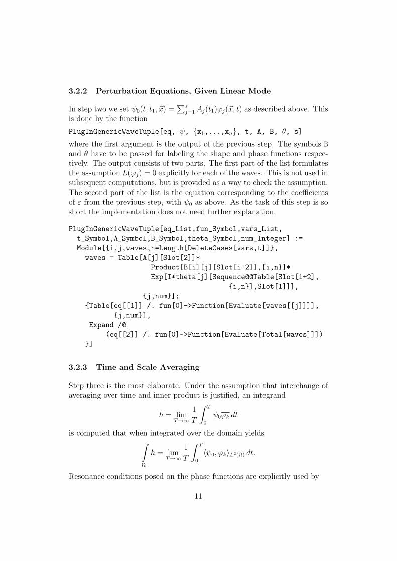
3.2.2 Perturbation Equations, Given Linear Mode

In step two we set ψ0(t, t1, ~x) =∑s

j=1 Aj(t1)ϕj(~x, t) as described above. Thisis done by the function

PlugInGenericWaveTuple[eq, ψ, x1,...,xn, t, A, B, θ, s]

where the first argument is the output of the previous step. The symbols B

and θ have to be passed for labeling the shape and phase functions respec-tively. The output consists of two parts. The first part of the list formulatesthe assumption L(ϕj) = 0 explicitly for each of the waves. This is not used insubsequent computations, but is provided as a way to check the assumption.The second part of the list is the equation corresponding to the coefficientsof ε from the previous step, with ψ0 as above. As the task of this step is soshort the implementation does not need further explanation.

PlugInGenericWaveTuple[eq_List,fun_Symbol,vars_List,

t_Symbol,A_Symbol,B_Symbol,theta_Symbol,num_Integer] :=

Module[i,j,waves,n=Length[DeleteCases[vars,t]],

waves = Table[A[j][Slot[2]]*

Product[B[i][j][Slot[i+2]],i,n]*

Exp[I*theta[j][Sequence@@Table[Slot[i+2],

i,n],Slot[1]]],

j,num];

Table[eq[[1]] /. fun[0]->Function[Evaluate[waves[[j]]]],

j,num],

Expand /@

(eq[[2]] /. fun[0]->Function[Evaluate[Total[waves]]])

]

3.2.3 Time and Scale Averaging

Step three is the most elaborate. Under the assumption that interchange ofaveraging over time and inner product is justified, an integrand

h = limT→∞

1

T

∫ T

0

ψ0ϕk dt

is computed that when integrated over the domain yields∫

Ω

h = limT→∞

1

T

∫ T

0

〈ψ0, ϕk〉L2(Ω) dt.

Resonance conditions posed on the phase functions are explicitly used by

11

Resonance[eq, linwav, x1,..,xn, t,

λ1,..,λp, A, B, θ, s, cond, k]

which receives the output from the previous step in eq. Here cond specifiesthe resonance condition in terms of the θj, which have to be entered asθ[j][x1,..,xn,t] respectively. The last argument is the index of the waveϕk in the integral above. Alternatively Resonance2 uses explicit parametersettings paramvalues for the waves instead of cond. This has been necessarybecause the general Resonance does not give useable results (see Section 3.3for more details). The main work in this step is to find out which terms donot contribute to the result. We exploit the fact that oscillating terms vanishwhen averaged over time by simply omitting those summands of 〈ψ0, ϕk〉L2(Ω)

that have a factor exp(iθ) with some time-dependent phase θ. The code forResonance is not shown here, but is quite similar to Resonance2.

Resonance2[eq_List,linwav_List,vars_List,t_Symbol,params_List,

A_Symbol,B_Symbol,theta_Symbol,num_Integer,

paramvalues_List,testwave_Integer] :=

Module[e,i,j,n=Length[DeleteCases[vars,t]],

e = Expand[(List@@Last[eq])*

Exp[-I*theta[testwave][Sequence@@

DeleteCases[vars,t],

t]]];

e = e /.

Table[

theta[j] ->

(Evaluate[(linwav[[n+1]] /.

(Rule@@#& /@

Transpose[params,paramvalues[[j]]]

)

) /. Append[Table[

DeleteCases[vars,t][[i]]

-> Slot[i],

i,n],

t -> Slot[n+1]]

]&

),

j,num];

e = MapAt[

(Function[theta,If[FreeQ[theta,t],theta,0]

]

12

[Simplify[#]]

)&,

e,

Position[e,Exp[_]]];

e = Equal@@

(e*Conjugate[A[testwave]][t[1]]*

Product[Conjugate[B[i]

[testwave]

[DeleteCases[vars,t][[i]]]

],

i,n]

) /.

Flatten[

Table[B[i][j] ->

Function[

Evaluate[DeleteCases[vars,t][[i]]],

Evaluate[linwav[[i]] /.

(Rule@@#& /@

Transpose[

params,paramvalues[[j]]

]

)]],

i,n,j,num]]

]

The integration of h is done by Mathematica and can be quite time-consuming.So ODESystem simplifies the integrand first to make integration faster. Stillthe expressions involved can be quite complicated. This is the most time-consuming part during construction of the ODEs.

3.3 Obstacles

Mathematica sometimes does not seem to take care of special cases and con-sequently has problems with evaluating expressions depending on symbolicparameters. We give two simple examples to illustrate this issue:

• Orthogonality of sine-functions.Indeed, it holds that

∀m,n ∈ N :

∫ 2π

0

sin(mx) sin(nx)dx = πδm,n.

13

Computing this in Mathematica by

Integrate[Sin[m*x]Sin[n*x], x,0,2π,Assumptions → m∈Integers && n∈Integers]

yields 0 independently of m,n instead.

• Computation of a limit.Mathematica evaluates an expression

∀n ∈ Z : limx→n

sin(xπ)

x= πδn,0

and similar expressions in two different ways getting two different an-swers. On the one hand

Limit[Sin[(m-n)π]/(m-n), m→n,

Assumptions → m∈Integers && n∈Integers]gives 0. On the other hand, however, when the condition m,n ∈ Zis not used for computing the result Mathematica yields the correctanswer π, as with

Limit[Sin[(m-n)π]/(m-n), m→n].

Unfortunately these issues prevented us from obtaining a nice formula forthe coefficients in symbolic form by Resonance. So we just compute resultsfor explicit parameter settings using Resonance2.

3.4 Results

3.4.1 Atmospheric Planetary Waves

For the validation of our program we consider the barotropic vorticity equa-tion on the sphere first. Here numerical values of the coefficients αi areavailable (Table 1, [16]). The equation looks quite similar

∂4ψ

∂t+ 2

∂ψ

∂λ= −εJ(ψ,4ψ)

However in spherical coordinates (φ ∈ [−π2, π

2], λ ∈ [0, 2π]) the differential

operators are different:

4 =∂2

∂φ2+

1

cos(φ)2

∂2

∂λ2− tan(φ)

∂

∂φ

14

J(a, b) =1

cos(φ)

(∂a

∂λ

∂b

∂φ− ∂a

∂φ

∂b

∂λ

).

The linear modes have in this case the following form [14]

Pmn (sin(φ)) exp(i(mλ +

2m

n(n + 1)t)) (5)

where Pmn (µ) are the associated Legendre polynomials of degree n and order

m ≤ n, so again they depend on the two parameters m and n. Also resonanceconditions on the parameters look different in this case.

Now we compute the coefficient α3 in (2). In [16] we find the followingequation for the amplitude A3

n3(n3 + 1)∂A3

∂t1(t1) = 2iZ(n2(n2 + 1)− n1(n1 + 1))A1(t1)A2(t1)

so α3 = 2iZ n2(n2+1)−n1(n1+1)n3(n3+1)

. Parameter settings and corresponding numer-

ical values for Z were taken from the table below (see [16]). For this equa-tion and s = 3 results produced by our program have the form c1A3A3 =c2A1A2A3, so α3 = c2/c1.

Testing all resonant triads from the Table 1 from [16], we see that the coeffi-cients differ merely by a constant factor of ±√8 which is due to the differentscaling of the Legendre polynomials. In our computation they were nor-malized s.t.

∫ 1

−1Pm

n (µ)2dµ = 1. With three triads, however, results werecompletely different. Interestingly this were exactly those triads for whichno ϕ0 appears in the table.

Furthermore, for the other coefficients in (2) our program computes α1 =α2 = 0 in all tested parameter settings. This fact can be easily understoodin the following way. We checked only resonance conditions but not theconditions for the interaction coefficients to be non-zero which are elaboratedenough:

mi ≤ ni, ni 6= nj ∀i = 1, 2, 3, |n1 − n2| < n3 < n1 + n2,

andn1 + n2 + n3 is odd.

Randomly taken parameter setting does not satisfy these conditions.

15

3.4.2 Ocean Planetary Waves

Returning to the original example on the domain [0, Lx] × [0, Ly], we findexplicit formulae for the coefficients in [15]. According to Section 3.3 we canonly verify special instances and not general formulae.

Linear modes have now the form [15]

sin(πmx

Lx

) sin(πny

Ly

) exp(i(β

2ωx + ωt)) (6)

with m,n ∈ N and ω = β

2πq

( mLx

)2+( nLy

)2.

Parameter settings solving the resonance conditions were computed as insection 4. Unfortunately results do not match and we have no explanationfor that. In particular the condition α1

ω21

+ α2

ω22

+ α3

ω23

= 0 stated in [15] does not

hold for the results of our program since we got α1 = α2 = 0 in all testedparameter settings, just as in the spherical case.

For example, if we try the triad 2,4,4,2,1,2 where Lx = Ly = 1

our program computes α3 = 32√

511

π(sin(3

√5π)− i(1 + cos(3

√5π))

), whereas

the general formula yields α3 = 19+7√

511

π sin(3√

5π). However, if we use a triadwith q = 1, e.g. 24,18,9,12,8,6, both agree on α1 = α2 = α3 = 0.

4 Resonance Conditions

The main equation to solve is

1√(m1

Lx)2 + ( n1

Ly)2

+1√

(m2

Lx)2 + ( n2

Ly)2

=1√

(m3

Lx)2 + ( n3

Ly)2

for all possible mi, ni ∈ Z with the scales Lx and Ly (also ∈ Z ) and thento check the condition n1 ± n2 = n3. In the following argumentation it willbe seen that Lx and Ly can be assumed to be free of common factors. Belowwe refer to Lx and Ly as to the scale coefficients.

The first step of the algorithm implemented in Mathematica is to rewritethe equation to 1√

m12+n1

2+ 1√

m22+n2

2= 1√

m32+n3

2and transform it in the

following way: we factorize the result of each mi2 + ni

2 and obtain withρ1 · . . . ·ρr being the factors of m2

i +n2i and α1 · . . . ·αr their respective powers:

m2i + n2

i = ρα11 · ρα2

2 · . . . · ραrr .

16

We will now define a weight γi of the wave-vector (mi, ni) as the productof the ρj’s to the quotient of their respective αj and 2. The weight qi will bethe name of the product of the ρj’s which have an odd exponent:

√m2

i + n2i = γi

√qi.

Our equation then can be re-written as

1

γ1√

q1

+1

γ2√

q2

=1

γ3√

q3

and one easily sees that the only way for the equation to possibly hold isq1 = q2 = q3 = q (see [12] for details). Further we call q an index of thecorresponding wave-vectors. The set of all wave-vectors with the same indexis called a class of index q and is denoted as Clq. Obviously, the solutionsof the resonance conditions are to be searched for with separate classes only.

At this point one can also see that only such scales, Lx and Ly, withoutcommon factors are reasonable. If they had a common factor, it would cancelout in the equation.

4.1 Method Description

The following five steps are the main steps of the algorithm:

• Step 1: Compute the list of all possible indexes q.

To compute the list of all indexes q, we use the fact that they have tobe square-free and each factor of q has to be different from 3 mod 4(Lagrange theorem). There exist 57 possible possible indexes in ourcomputational domains q ≤ 300 :

1, 2, 5, 10, 13, 17, 26, 29, 34, 37, 41, 53, 58, 61, 65, 73, 74, 82, 85, 89,

97, 101, 106, 109, 113, 122, 130, 137, 145, 146, 149, 157, 170, 173, 178,

181, 185, 193, 194, 197, 202, 205, 218, 221, 226, 229, 233, 241, 257,

265, 269, 274, 277, 281, 290, 293, 298

• Step 2: Solve the weight equation 1γ1

+ 1γ2

= 1γ3

.

For solving the weight equation, we transform it into the equivalentform:

γ3 =γ1 γ2

γ1 + γ2

(7)

17

The solution triples γ1, γ2, γ3 can now be found by the two for-loopsover γ1 and γ2 up to a certain maximum parameter and γ3 is then beingfounded constructively with formula (7).

• Step 3: Compute all possible pairs (mi, ni) - if there are any - thatsatisfy m2

i + n2i = γ2

i q.

To compute our initial variables mi, ni, we use the Mathematica stan-dard function SumOfSquareRepresentation[d, x] which produces alist of all possible representations of an integer x as a sum of d squares,i.e. we can find all possible pairs (a, b) with d = 2 such that theysatisfy a2 + b2 = x. Therefore, checking the condition m2

i + n2i = γ2

i qis easy.

• Step 4: Sort out the solutions m1, n1,m2, n2,m3, n3 that do notfulfill the condition n1± n2 = n3.

• Step 5: Check if by dividing the mi by Lx and the ni by Ly there arestill exist some solutions.

Last two steps are trivial.

4.2 The Implementation

Our implementation is quite straightforward and the main program is basedon 4 auxiliary functions shown in the following subsections.

4.2.1 List of Indexes

The function constructqs[max] produces the list of all possible indexes qup to the parameter max. The first (obvious) q’s sol = 1 is given and thefunction checks the conditions starting with n = 2. Every time n satisfiesthe conditions, it is appended to the list sol. If one condition fails, the nextn = n + 1 is considered and so on until n reaches the parameter max. Thenthe list sol is returned:

Clear[constructqs];

constructqs[n , sol List, max ]; n>max := sol (*6*)

constructqs[n ?SquareFreeQ, sol List, max ]

:= constructqs[n+1, Append[sol, n], max] (*5*)

18

constructqs[n ?SquareFreeQ, sol List, max ];

MemberQ[Mod[PrimeFactorList[n], 4], 3]

:= constructqs[n+1, sol, max] (*4*)

constructqs[n , sol List, max ]; !SquareFreeQ[n]

:= constructqs[n+1, sol, max] (*3*)

constructqs[1] := 1 (*2*)

constructqs[max ] := constructqs[3, 1, max] (*1*)

4.2.2 Weight Equation

The function findγs[γmax] solves the weight equation in the following way.For a fixed γ1 and γ2 running between 1 and γmax, it is checked if γ3 isan integer. If it is, the triple γ1, γ2, γ3 is added to the list sol which isempty at the initial moment. Once γ2 reaches γmax, it is set to 1 againand the search starts again with γ1 = γ1 + 1. This is done as long as bothγ1 and γ2 are lower than max. Finally the list sol is returned:

findγs[γmax , γ1 , γ2 , sol List];

γ1 > γmax := (Clear[γ3],sol) (*6*)

findγs[γmax , γ1 , γ2 , sol List]; (γ1 ≤ γmax && γ2>γmax &&

IntegerQ[γ3=(γ1γ2)/(γ1+γ2)]):= findγs[γmax, γ1+1, 1, Append[sol, γ1, γ2, γ3]] (*5*)

findγs[γmax , γ1 , γ2 , sol List];

(γ1 ≤ γmax && γ2>γmax &&

!IntegerQ[γ3=(γ1γ2)/(γ1+γ2)]):= findγs[γmax, γ1 + 1, 1, sol] (*4*)

findγs[γmax , γ1 , γ2 , sol List];

(γ1 ≤ γmax && γ2 ≤ γmax && IntegerQ[γ3=(γ1γ2)/(γ1+γ2)]):= findγs[γmax, γ1, γ2 + 1, Append[sol, γ1, γ2, γ3]] (*3*)

findγs[γmax , γ1 , γ2 , sol List];

(γ1 ≤ γmax && γ2 ≤ γmax && !IntegerQ[γ3=(γ1γ2)/(γ1+γ2)]):= findγs[γmax, γ1, γ2 + 1, sol] (*2*)

findγs[γmax ] := findγs[γmax, 1, 1, ]) (*1*)

For findγs[γmax] to be executable, the iteration depth of 212 is not sufficientand it was set to ∞.

19

4.2.3 Linear Condition

The third auxiliary function makemns checks whether the linear conditionn1 ± n2 = n3 is fulfilled and structures the solution set into a list of pairsm1, n1, m2, n2, m3, n3 :

Clear[makemns];

makemns[m1 , n1 , m2 , n2 , m3 , n3 ] := (*3*)

makemns[m1 , n1 , m2 , n2 , m3 , n3 ];

(n1 + n2 == n3 ‖ n1 - n2 == n3) :=

m1, n1, m2, n2, m3, n3 (*2*)

makemns[mn1 List, mn2 List, mn3 List] :=

Cases[Flatten[Table[makemns[mn1[[i,1]], mn1[[i,2]],

mn2[[j,1]], mn2[[j,2]], mn3[[k,1]], mn3[[k,2]]],

i, 1, Length[mn1], j, 1, Length[mn2],k, 1, Length[mn3]], 2],

x1 ,x2 , x3 ,x4 , x5 ,x6 ] (*1*)

The function makemns is called three times:

In (*1*) from 3 lists of arbitrarily many pairs mi, ni, a 3-dimensionalarray is made combining entries of the 3 lists with each other. Each entrycalls the same program with the parameters of the current combination ofm1,n1,m2,n2,m3,n3.In (*2*) and (*3*) it is decided whether the condition n1 ± n2 = n3is fulfilled. If it is, a solution m1,n1,m2,n2,m3,n3 is written inthe array. The table is then flattened to the level 2 in order to have alist of solutions. In the end, all empty lists have to be sorted out, doneby the function Cases which keeps only those cases that have the shapex1 ,x2 ,x3 ,x4 ,x5 ,x6 .

4.2.4 Scale Coefficients

Finally, the function respectL[sol, Lx, Ly] divides each component of thesolution by the pair (Lx, Ly) and sorts out the result if any of the 6 compo-nents does not remain an integer:

respectL[sol List, Lx , Ly ] :=

Map[solution[#]&,

Cases[Map[#/Lx, Ly&,Map[#[[1]]]&, sol], 2], Integer, Integer, Integer, Integer, Integer, Integer]]

20

The function respectL[sol, Lx, Ly] gets as an input the list of the formsolution[m1,n1,m2,n2,m3,n3],... and returns the list of the sameform.

4.3 Results

All solutions in the computation domain m,n ≤ 300 have been found ina few minutes. Notice that computations in the domain m,n ≤ 20 bydirect search, without introducing indexes q and classes Clq took about30 minutes. A direct search in the domain m,n ≤ 30 has been interruptedafter 2 hours, since no results were produced.

The number of solutions depends drastically on the scales Lx and Ly,some data are given below (for the domain m,n ≤ 50 : )

(Lx = 1, Ly = 1) : 76 solutions;

(Lx = 3, Ly = 1) : 23 solutions;

(Lx = 6, Ly = 16) : 2 solutions;

(Lx = 5, Ly = 21) : 2 solutions;

(Lx = 11, Ly = 29) : no solutions (search up to 300, for both qmax andγmax).

Interestingly enough, in all tried possibilities, only an odd q yield solutions.

5 Structure of the Solution Set

5.1 Method Description

The graphical way to present 2D-wave resonances suggested in [9] for 3-wave

interactions is to regard each 2D-vector ~k = (m,n) as a node (m,n) of inte-ger lattice in the spectral space and connect those nodes which construct onesolution (triad, quartet, etc.). Having computed already all the solutions of(3) in Section 4, now we are interested in the structure of resonances in spec-tral space. To each node (m,n) we can prescribe an amplitude A(m,n, t1)whose time evolution can be computed from the dynamical equations ob-tained in Section 3. Thus, solution set of resonance conditions (3) can bethought of as a collection of triangles, some of them are isolated, some formsmall groups connected by one or two vertices. Corresponding dynamical

21

systems can be re-constructed from the structure of these groups. For in-stance, a single isolated triangle corresponding to a solution with wave vectors(m1, n1)(m2, n2)(m3, n3) and wave amplitudes (A1, A2, A3) corresponds tothe following dynamical system:

A1 = α1A2A3

A2 = α2A1A3

A3 = α3A1A2

with αi being functions of all mi, ni (see Section 3).

If that two triangles share one common vertex (A1, A2, A3), (A3, A4, A5),the the corresponding dynamical system is

A1 = α1A2A3

A2 = α2A1A3

A3 = α3,1A1A2 + α3,2A4A5

A4 = α4A3A5

A5 = α5A3A4

If two triangles have two vertices in common (A1, A2, A3), (A2, A3, A4),then the dynamical system is quite different:

A1 = α1A2A3

A2 = α2,1A1A3 + α2,2A3A4

A3 = α3,1A1A2 + α3,2A2A4

A4 = α4A2A3 =α4

α1

A1

Using the fourth equation, the formulae for A2 and A3 can be simplified to:

A4 =α4

α1

A1 ⇒ A4 =α4

α1

A1 + β1

A2 = A1A3

(α2,1 +

α2,2α4

α1

)+

α4β1

α1

A3 = A1A2

(α3,1 +

α3,2α4

α1

)+

α4β1

α1

This means that qualitative dynamics of the 3-term mesoscopic system de-pends not on the geometrical structure of the solution set but on its topologicalstructure. Constructing the topological structure of the solution set, we do

22

not consider concrete values of the solution but only the way how trianglesare connected. In any finite spectral domain we can compute all independentwave clusters and write out corresponding dynamical systems thus obtain-ing complete information about energy transfer through the spectrum. Ofcourse, quantitative properties of the dynamical systems depend on the spe-cific values of mi, ni (for instance, values of interaction coefficients αi,magnitudes of periods of the energy exchange among the waves belonging toone cluster, etc.)

5.2 Implementation

To construct the topological structure of a given solution set we need first tofind all groups of connected triangles. This is done by the following proce-dure:

FindConnectedGroups[triangles_List] :=

Block[groups = , tr = triangles, newgroup,

While[Length[tr] > 0,

newgroup, tr =

FindConnectedTriangles[First[tr], Rest[tr]];

groups = Append[groups, newgroup];

];

groups

];

FindConnectedTriangles[grp_List,triangles_List]:=

Module[points,newGrpMember,tr=triangles,

points=Flatten[Apply[List,grp,2],1];

newGrpMember=Cases[tr, _[___,#1,___]]&/@points;

(tr=DeleteCases[tr, _[___,#1,___]])&/@points;

newGrpMember=Union[Join@@newGrpMember];

If[Length[newGrpMember]==0,

grp,tr,

newGrpMember=FindConnectedTriangles[newGrpMember,tr];

Join[grp,First[newGrpMember]],

newGrpMember[[2]]

]

];

The function FindConnectedGroups expects a list of triangles as input, andthree different types for data structure can be used. The first type is just

23

a list of three pairs, where each pair contains the coordinates of a node, forexample 1,2,3,4,5,6. An alternative type is like the type beforejust with another head symbol instead of list, e.g.Triangle[1,2,3,4,5,6].

The function also works for vertex numbers instead of coordinates, e.g.Triangle[1, 2, 3]. In every case the function returns a partition of theinput list where all elements of a list are connected and elements of differentlists have no connection to each other.

The function FindConnectedTriangles is an auxiliary function which hastwo parameters. The first list contains allconnected triangles. The secondlist contains all other triangles which are possibly connected to one of thetriangles in the first list. The function FindConnectedTriangles returns apair of lists: the first list contains all triangles which are connected to theselected triangles, the second list contains all remaining.

The input list for FindConnectedTriangles is a list of 3-element lists. Beforewe can use the results produced in Section 4 as an input we have to transformthe data. This can be easily done by:

TransformSolution[sol_List]:=

Flatten[Rest/@sol]/.solution[trs:___List]->trs;

Some remarks on the implementation.

The function FindConnectedGroups selects a triangle, which is not yet in agroup and calls the function FindConnectedTriangles. Since the returnedfirst list always contains at least one triangle, the length of the list tr de-creases in every loop call, hence the FindConnectedGroups terminates. Thequestion left is how to find all triangles connected with a certain triangle.This has been done in the following way. First we search for all triangleswhich share at least one node with this triangle. Then we restart the searchwith all triangles found. For efficiency reasons it is better to perform thesearch with all triangles we found in one step together. If in one step no fur-ther triangles are found then we are ready and return the list of connectedtriangles and the remaining list. In each step we remove all triangles wefound from the list of triangles which are not declared as connected. Thisincreases the speed because the search is faster if there are less elements tocompare. More important, this prevent us to search in loops and find sometriangles more than once. In general, search in a loop can be the reason fora termination problem but due to shrinking the list of triangles to search forin every step the termination can be guaranteed.

24

5.3 Results

In the Figure 1 the geometrical structure of the solution set is shown, for thecase mi, ni ≤ 50 and Lx = Ly = 1.

10 20 30 40 50

10

20

30

40

50

Figure 1: The geometrical structure of the result in domain D = 50

Below we show all the topological elements of this solution set.

1. 21 groups contain only one triangle (obviously, they have isomorphicdynamical systems):

3, 18, 36, 6, 2, 12 4, 46, 14, 44, 23, 26, 44, 36, 26, 13, 18 6, 48, 42, 24, 3, 248, 26, 16, 22, 13, 4 9, 24, 48, 18, 16, 614, 28, 28, 14, 7, 14 18, 36, 36, 18, 9, 1822, 16, 26, 8, 11, 8 22, 20, 28, 10, 11, 1022, 44, 44, 22, 11, 22 22, 48, 42, 32, 21, 1624, 18, 9, 12, 8, 6 26, 28, 28, 26, 19, 228, 42, 42, 28, 21, 14 28, 46, 50, 20, 7, 2636, 22, 42, 4, 11, 18 36, 30, 15, 18, 10, 1238, 24, 42, 16, 21, 8 44, 18, 46, 12, 23, 648, 36, 18, 24, 16, 12

2. Further 9 groups contain also one triangle, but in each triangle two points

25

coincide (again, they have isomorphic dynamical systems):

8, 2, 8, 2, 1, 4 16, 2, 16, 2, 7, 416, 4, 16, 4, 2, 8 24, 6, 24, 6, 3, 1232, 8, 32, 8, 4, 16 34, 8, 34, 8, 7, 1646, 8, 46, 8, 17, 16 48, 6, 48, 6, 21, 1248, 12, 48, 12, 6, 24

3. There exist 2 groups with two triangles each (by observation of the geo-metrical pictures it is easy to determine that both have isomorphic dynamicalsystems):

2, 24, 18, 16, 9, 8, 4, 48, 36, 32, 18, 16 12, 26, 26, 12, 3, 14, 26, 12, 28, 6, 13, 6

4. Two further groups consist of two triangles each, but the common point iscontained twice in one triangle (the dynamical systems are isomorphic, butdifferent from the two groups above):

24, 22, 32, 6, 3, 16, 32, 6, 32, 6, 11, 12 8, 38, 32, 22, 11, 16, 38, 8, 38, 8, 11, 16

5. As we can see by inspecting their geometrical structures, further 7 groupsare not isomorphic to any group found above:

6, 12, 12, 6, 3, 6, 12, 24, 24, 12, 6, 12,24, 48, 48, 24, 12, 24

2, 16, 14, 8, 1, 8, 4, 32, 28, 16, 2, 16,32, 4, 32, 4, 14, 8

2, 4, 4, 2, 1, 2, 4, 8, 8, 4, 2, 4,8, 16, 16, 8, 4, 8, 16, 32, 32, 16, 8, 16

4, 22, 10, 20, 11, 2, 8, 44, 20, 40, 22, 4,10, 20, 20, 10, 5, 10, 20, 40, 40, 20, 10, 20

10, 40, 26, 32, 19, 8, 26, 32, 38, 16, 13, 16,32, 26, 40, 10, 13, 16, 40, 10, 40, 10, 5, 20

4, 18, 14, 12, 7, 6, 8, 36, 28, 24, 14, 12,12, 14, 14, 12, 9, 2, 24, 28, 28, 24, 18, 4,36, 42, 42, 36, 27, 6, 42, 36, 21, 18, 4, 18

26

2, 36, 20, 30, 17, 6, 4, 6, 6, 4, 3, 2,8, 12, 12, 8, 6, 4, 12, 18, 18, 12, 9, 6,16, 24, 24, 16, 12, 8, 18, 12, 9, 6, 4, 6,20, 30, 30, 20, 15, 10, 20, 30, 34, 12, 1, 18,24, 36, 36, 24, 18, 12, 30, 20, 36, 2, 1, 18,32, 48, 48, 32, 24, 16, 34, 12, 36, 2, 15, 10,36, 24, 18, 12, 8, 12, 45, 30, 34, 12, 12, 18

Geometrical interpretation of all topological elements is given below. Incases when there exist more then one element with given structure, wavenumbers are written at the picture corresponding to the element chosen forpresentation.

2 9 16 23 30 376

9

12

15

18

2,12

3,18

36,6

0 2 4 6 8

2

3

4

8,2

1,4

0 9 18 27 3608

1624324048

36,32

18,16

4,48

2,24

9,8

0 8 16 24 32

6

10

14

18

22

32,6

24,22

3,16

11,12

0 6 12 18 24 30 36 42 486

12182430364248

0 4 8 12 16 20 24 28 320

8

16

24

32

0 4 8 12 16 20 24 28 32048

121620242832

5 10 15 20 25 30 35 400

10

20

30

40

5 12 19 26 33 408

16

24

32

40

6 12 18 24 30 36 4206

121824303642

0 6 12 18 24 30 36 42 4806

12182430364248

27

5.4 Important Remark

To compute all non-isomorphic sub-graphs algorithmically is a nontrivialproblem. Indeed, all isomorphic graphs presented in previous section aredescribed by similar dynamical systems, only magnitudes of interaction co-efficients αi vary. However, in the general case graph structure thus defineddoes not present the dynamical system unambiguously. Consider Figure 2below where two objects are isomorphic as graphs. However, the first objectrepresents 4 connected triads with dynamical system

(A1, A2, A3), (A1, A2, A5), (A1, A3, A4), (A2, A3, A6) (8)

while the second - 3 connected triads with dynamical system

(A1, A2, A5), (A1, A3, A4), (A2, A3, A6). (9)

A1 A2

A3A4

A5

A6

A1 A2

A3A4

A5

A6

ì

Figure 2: Example of isomorphic graphs and non-isomorphic dynamical sys-tems. The left graph corresponds to the dynamical system (8) and the graphon the right - to the dynamical system (9). To discern between these twocases we set a placeholder inside the triangle not representing a resonance.

This problem has been solved in [17] by introducing hyper-graphs of a specialstructure; the standard graph isomorphism algorithm used by Mathematicahas been modified in order to suit hyper-graphs.

6 A Web Interface to the Software

The previous sections have presented implementations of various symboliccomputation methods for the analysis of non-linear wave resonances. Theseimplementations are written in the language of the computer algebra system

28

Mathematica which provides an appealing graphical user interface (GUI)for executing computations and presenting the results. For instance, thepictures shown in Section 4.3 were produced by converting the computedhyper-graphs to Mathematica plot structures that can be displayed by theGUI of the system.

However, to run these methods the user needs an installation of Mathematicaon the local computer with the previously described methods installed in alocal directory. These requirements make access to the software difficult andhamper its wide-spread usage. In order to overcome this problem, we haveimplemented a Web interface such that the software can be executed fromany computer connected to the Internet via a Web browser without the needfor a local installation of mathematical software.

This implementation follows a general trend in computer science which turnsaway from stand alone software (that is installed on local computers andcan be only executed on these computers via a graphical user interface) andproceeds towards service-oriented software [18] (that is installed on removeserver computers and wraps each method into a service that can be invokedover the Internet via standardized Web interfaces). Various projects in com-puter mathematics have pursued middleware for mathematical web services,see for instance [19, 20, 21]. On the long term, it is thus envisioned that math-ematical methods generally become remote services that can be invoked byhumans (or other software) without requiring local software installations.

However, even without sophisticated middleware it is nowadays relativelysimple to provide (for restricted application scenarios) web interfaces tomathematical software by generally available technologies. The web interfacepresented in the following sections is deliberately kept as simple as possibleand makes only use of such technologies; thus it should be easy to take thissolution as a blueprint for other mathematical software with similar features.In particular, the web interface is quite independent of Mathematica as thesystem underlying the implementation of the mathematical methods; thesame strategy can be applied to other mathematical software systems suchas Maple, MATLAB, etc.

6.1 The Interface

Figure 3 shows the web interface to some of the methods presented in theprevious sections. Its functionality is as follows:

Create Solution Set The user may enter a parameter D in the first (small)text field and then press the button “Create Solution Set”. This invokes

29

Figure 3: Web interface to the implementation

the method CreateSolutionSet which computes the set of all solutionswhose values are smaller than or equal to D. This set is written intothe second (large) text field in the form

Solution[x1,y1,z1],...,Solution[xn,yn,zn]Plot Topology The user may enter into the second (large) text field a spe-

cific solution set (or, as show above, compute one), and then pressthe button “Plot Topology”. This first invokes the method Topology

which computes the topological structure of the solution set as a listof hyper-graphs and then calls the method PlotTopology which com-putes a plot of each hyper-graph. The results are displayed in the rightframe of the browser window.

The web interface is available at the URL

http://www.risc.uni-linz.ac.at/projects/alisa

(Button “Discrete Wave Turbulence”)

To run the computations, an account and a password are needed.

30

6.2 The Implementation

The web interface is implemented in PHP, a scripting language for producingdynamic web pages [22]. PHP scripts can be embedded into conventionalHTML pages within tags of form <php?...?>; when a Web browser requestssuch a page, the Web server executes the scripts with the help of an embeddedPHP engine, replaces the tags by the generated output, and returns theresulting HTML page to the browser. With the use of PHP, thus programscan be be implemented that run on a web server and deliver their results toa client computer which displays them in a web browser. The web interfaceto the discrete wave turbulence package is implemented in PHP as sketchedin Figure 4 and described below (the parenthesized numbers in the text referto the corresponding numbers in the figure).

Create Solution Set The browser frame input on the left side containsessentially the following HTML input form:

<form target="textarea"action="https://apache2.../CreateSolutionSet.php"method="post">

<input name="domain" size="3"><input type="submit" value="Create Solution Set">

</form>

This form consists of an input field domain to receive a domain value anda button to trigger the creation of the solution set. When the button ispressed, (1) a request is sent to the web server which carries the value ofdomain; this request asks the server to deliver the PHP-enhanced web pageCreateSolutionSet.php into the target frame textarea which is displayedinternally to input.

The file CreateSolutionSet.php has essentially the content

<?php$math="/.../math";$cwd="/.../DiscreteWaveTurbulence";$domain = $_POST[’domain’];$mcmd ="SetDirectory[\"" . $cwd . "\"]; " ."Needs[\"DiscreteWaveTurbulence‘SolutionSet‘\"]; " ."sol=DiscreteWaveTurbulence‘SolutionSet‘CreateSolutionSet[" .

$domain . "]; ";

31

-

?

6

¾

resultinput

S

Mathematica

PHP EngineWeb Server/

Server Computer

Create Solution Set

Plot Topology

(1) D

Client Computer

D

CreateSolutionSet.php/

D (3)CreateSolutionSet[ ](2) S

textarea<html>.. ..</html>(4) S

resultinput

Mathematica

PHP EngineWeb Server/

Server Computer

Create Solution Set

Plot Topology

Client Computer

textarea

(1)

S

PlotTopology.php/S

PlotTopology[... ...]S(2)

(3) Export["image-1.png",...]

(4)

<html><img src="image-1.png">...

(6) GET image-1.png

N

(5)

Figure 4: Implementation of the web interface

32

$command="$math -noprompt -run ’" . $mcmd ."Print[StandardForm[sol]]; Quit[];’";

$result = shell_exec("$command");echo..."<textarea name=\"sol\" cols=\"60\" rows=\"20\">" .htmlspecialchars($result) ."</textarea>" .

...;?>

After setting the paths $math of the Mathematica binary and $cwd of thedirectory where the DiscreteWaveTurbulence package is installed, the scriptsets the local variable $domain to the value of the input field domain. Thenthe Mathematica command $mcmd is constructed in order to load the fileSolutionSet.m and execute the command CreateSolutionSet to computethe solution set. Now the system command $command is constructed to (2)invoke Mathematica which calls the previously constructed command and(3) prints its result to the standard output stream which is captured in thevariable $result. From this, the script contstructs the HTML code of theresult document which is (4) delivered to the Web browser.

Plot Topology The browser frame textarea contains essentially the fol-lowing HTML input form:

<form target="result"action="https://apache2..../PlotTopology.php"method="post">

<textarea name="sol" cols="60" rows="20">...</textarea><input type="submit" value="Plot Topology"></center>

</form>

This form consists of the textarea field sol to receive the solution set and abutton to trigger the plotting of the topology of this set. When the buttonis pressed, (1) a request is sent to the web server which carries the valueof sol; this request asks the server to deliver the PHP-enhanced web pagePlotTopology.php into the target frame result on the right side of thebrowser.

The file CreateSolutionSet.php has essentially the content

33

<?php$math="/.../math";$basedir ="/.../DiscreteWaveTurbulence";$baseurl ="http://apache2/.../DiscreteWaveTurbulence";$sol = $_POST[’sol’];... // create under $basedir a unique subdirectory $dir$mcmd ="SetDirectory[\"$basedir/$dir\"]; " ."Needs[\"DiscreteWaveTurbulence‘Topology‘\"]; " ."Needs[\"DiscreteWaveTurbulence‘SolutionSet‘\"]; " ."top=DiscreteWaveTurbulence‘Topology‘Topology[$sol]; " ."plots=DiscreteWaveTurbulence‘Topology‘PlotTopology1[top];";

$command="/usr/bin/Xvnc :20 & export DISPLAY=:20; " ."export MATHEMATICA_USERBASE=$basedir/.Mathematica; " ."$math -run ’" . $mcmd ."Print[ExportList[plots,\"$image\"]]; Quit[];’";

$result = shell_exec("$command | tail -n 1");for ($i=0;$i<$result;$i++)echo "<img src=\"$baseurl/$dir/image-$i.png\"/>";

?>

For holding the images to be generated later, the script creates a uniquedirectory $basedir/$dir which is served by the web server under the url$baseurl/$dir. The script extracts the solution set $sol from the requestand sets up the Mathematica command to compute its topological structureand generate the plots from which ultimately the image files will be produced.

For this purpose, however, Mathematica needs an X11 display server running;since a Web server has not access to an X11 server, we start the virtual X11server Xvnc [23] as a replacement and set the environment variable DISPLAY

to the display number on which the number listens; Mathematica will subse-quently send X11 requests to that display which will be handled by the virtualserver. Likewise, Mathematica needs access to a .Mathematica configurationdirectory; the script sets the environment variable MATHEMATICA USERBASE

correspondingly.

With these provisions, we can (2) invoke first the command to computethe plots and then the (self-defined) command ExportList to generate forevery plot an image in the previously created directory. For this purpose thecommand uses (3) the Mathematica command EXPORT[file,plot,"PNG"]

which converts plot to an image in PNG format and writes the image to file.ExportList returns the number of images generated which is (4) writtento the standard output stream which in turn is captured in the variable

34

$result. From this information, the script generates an HTML documentwhich contains a sequence of img elements referencing these images. Afterthis document has been (5) returned to the client browser, the browser (6)requests the referenced images with GET messages from the web server.

6.3 Extensions

As an alternative to the display of static images, the Web interface alsoprovides an option “Applet Viewer” with somewhat more flexibility. If thisoption is selected, Mathematica is instructed to save all generated plots asfiles in the standard representation. The generated HTML document thenembeds (rather than img elements) a sequence of applet elements that loadinstances of the “JavaView” applet [24]. These applets run in the Java Vir-tual Machine of the Web browser on the client computer, load the plot filesfrom the web, and visualize them in the browser. Rather than just displayingstatic images, the viewer allows to perform certain manipulations and trans-formations of the plots such as scaling, rotating, etc. While this additionalflexibility is not of particular importance for the presented methods, theymay in the future become useful for others.

To limit access to the software respectively to the computing power of theserver computer, it may be protected by authentication mechanisms. Forexample, on the Apache Web server, it suffices to provide in the installationdirectory of the software a file .htaccess with content

<Files "*.php">SSLRequireSSLAuthName "your account"AuthType BasicRequire valid-user

</Files>

With this configuration, the user is asked for the data of a valid accounton the computer running the Web server; other authentication mechanismsbased e.g. on password files may be provided in a similar fashion.

7 Discussion

Summing up all the results obtained, we would like to make some concludingremarks.

35

• In general, coefficients αi can be computed symbolically by hand andonly numerically by Mathematica (see Section 3.3); at present we arenot aware of the possibility to overcome this problem.

• For the known case of spherical barotropic vorticity equation, valuesof coefficients αi coincide with known form the literature for all triadsbut three. These 3 triads, though satisfying resonant conditions, areknown to be special from the physical point of view in the followingsense (see [16] for details). Though resonance conditions are fulfilledfor the waves of these triads, they, so to say, do not have a place in thephysical space to interact and their influence (if any) on the dynamicsof the wave system has to be studied separately from all other waves.Our results might indicate that also the coefficients αi of these triadshave to be defined in some other way compare to other resonant triads.For instance, another way of space-averaging has to be chosen.

• The results of Section 3.4.2 show that analytical formulae given in [15]for αj are not correct.

• The results of Section 4.3 show a crucial dependence of the numberof solutions on the form of the boundary conditions. In particular,some boundary conditions (for example, (Lx, Ly) = (11, 29)) yield nosolutions which is of most importance for physical applications. Fromthe mathematical point of view, an interesting result has been observed:in all our computations (i.e. for m,n ≤ 300) indexes correspondingto non-empty classes, turned out to be odd. It would be interesting toprove this fact analytically because if it keeps true, we can reduce thecomputational time.

• The algorithm presented in Section 4 has been implemented beforenumerically in Visual Basic, and our purpose here was to show that itworks fast enough also in Mathematica. The algorithms presented inSection 3 and Section 5 have never been implemented before, the wholework is usually done by hand and some mistakes as in [15] are almostunavoidable: it takes sometimes a few weeks of skillful researchers tocompute interaction coefficients of dynamical systems for one specificwave system.

• All the algorithms presented above can easily be modified for the caseof a 4-term mesoscopic system. The only problem left is a procedureto establish all non-isomorphic topological elements for a quadruplegraphs, similar to the procedure given in [17] for a triangle graphs.

36

The structure of quadruple graphs is much more complicated whilesome mechanisms of energy transfer in the spectral space do exist [25]that are absent in 3-term mesoscopic systems. A complete classificationof quadruple graphs is still an open question but in a given spectraldomain it can be done directly (a very time consuming operation).

• We have developed a Web interface for the presented methods, whichturns the implementations from only locally available software to Web-based services that can be accessed from any computer in the Internetthat is equipped with a Web browser. The presented implementationstrategy is simple and based on generally available technologies; it canbe applied as a blueprint for a large variety of mathematical software.In particular, the results are not bound to the current Mathematicaimplementation but can be adapted to any other computer algebrasystem (e.g. Maple) or numerical software system (e.g. MATLAB) ofsimilar expressiveness.

• At present, an explicit form of eigen-modes (5), (6) is used as one ofthe input parameters for our program package. Theoretically, at leastfor some classes of linear partial differential operators and boundaryconditions, computing eigen-modes can also be performed symbolicallybasing on the results in [26]. If this were done, not an eigen-mode butboundary conditions would play role of input parameter.

Acknowledgements. Authors acknowledge the support of the AustrianScience Foundation (FWF) under projects SFB F013/F1301 ”Numerical andsymbolical scientific computing”, P20164-N18 ”Discrete resonances in nonlin-ear wave systems” and P17643-NO4 ”MathBroker II: Brokering DistributedMathematical Services”.

References

[1] M. Cheney. Tesla Man Out Of Time (Dorset Press, 1989)

[2] G.P. Berman, F.M. Israilev. ”The Fermi-Pasta-Ulam problem: Fiftyyears of progress.” Chaos 15 (1), pp. 015104-015104-18 (2005)

[3] V. Zakharov, F. Dias, A. Pushkarev. ”One-dimensional wave turbu-lence.” Physics Reports 398, pp.1-65 (2004)

37

[4] V.E. Zakharov V.E., V.S. L’vov, G. Falkovich. Kolmogorov Spectraof Turbulence. Series in Nonlinear Dynamics, Springer (1992)

[5] V.E. Zakharov, N.N. Filonenko. ”Weak turbulence of capillary waves.”J.Appl. Mech. Tech. Phys. 4, pp.500-515 (1967)

[6] A.N. Pushkarev, V.E. Zakharov. ”Turbulence of capillary waves - theoryand numerical simulations.” Physica D 135, pp.98-116 (2000)

[7] V.E. Zakharov, A.O. Korotkevich, A.N. Pushkarev, A.I. Dyachenko.”Mesoscopic wave turbulence.” JETP Letters, 82 (8), 491 (2005)

[8] M. Tanaka. ”On the role of resonant interactions in the short-term evolu-tion of deep-water ocean spectra.” J. Phys. Oceanogr. 37, pp.1022-1036(2007)

[9] E.A. Kartashova ”Wave resonances in systems with discrete spectra”.In book: V.E. Zakharov (Ed.) Nonlinear Waves and Weak Turbu-lence, pp.95-129 (Series: Advances in the Mathematical Sciences, AMS,1998)

[10] E. Kartashova. ”A model of laminated turbulence.” JETP Letters 83(7), pp. 341-345 (2006)

[11] A.N. Nayfeh. Introduction to perturbation techniques. Wiley-Interscience, NY (1981)

[12] E. Kartashova. ”Fast Computation Algorithm for Discrete Resonancesamong Gravity Waves”. Low Temp. Phys. 145 (1-4), pp. 286-295 (2006)

[13] E. Kartashova, A. Kartashov. ”Laminated wave turbulence: generic al-gorithms I”. Int. J. Mod. Phys. C 17(11), pp. 1579-1596 (2006); ”Lam-inated wave turbulence: generic algorithms II”. Comm. Comp. Phys.2 (4), pp. 783-794 (2007); ”Laminated wave turbulence: generic algo-rithms III”. Physics A: Stat. Mech. Appl. 380, pp. 66-74 (2007)

[14] J. Pedlosky. Geophysical Fluid Dynamics (Springer, 1987)

[15] E.A. Kartashova, G.M. Reznik. ”Interactions between Rossby waves inbounded regions.” Oceanology 31, pp.385-389 (1992)

[16] E. Kartashova, V.S. L’vov. ”A model of intra-seasonal oscillations in theEarth atmosphere.” Phys. Rev. Lett. 98 (19): 198501 (2007) (featuredin Nature Physics 3(6): 368, 2007)

38

[17] E. Kartashova, G. Mayrhofer. ”Cluster formation in mesoscopic sys-tems”. Physica A: Stat. Mech. Appl. 385, pp. 527-542 (2007)

[18] N. Gold, A. Mohan, C. Knight, M. Munro. “Understanding service-oriented software” IEEE Software, 21(2): 71–77, March–April 2004.

[19] MathBroker II: Brokering Distributed Mathematical Services ReseachInstitute for Symbolic Computation (RISC), 2007. http://www.risc.uni-linz.ac.at/projects/mathbroker2.

[20] MONET — Mathematics on the Web. The MONET Consortium, April2004. http://monet.nag.co.uk.

[21] R. Baraka, W. Schreiner. “Semantic Querying of Mathematical WebService Descriptions”. Third International Workshop on Web Servicesand Formal Methods (WS-FM 2006), Vienna, Austria, September 8–9,2006. M. Bravetti, et al. (eds.), Lecture Notes in Computer Science 4184,pp. 73-87. Springer.

[22] The PHP Group. “PHP: Hypertext Preprocessor”. http://www.php.net,2007.

[23] RealVNC Remote Control Software. “VNC Free Edition 4.1”.http://www.realvnc.com/products/free/4.1, 2007.

[24] The JavaView Project. “JavaView — Interactive 3D Geometry and Vi-sualization”. http://www.javaview.de, 2007.

[25] E. Kartashova. ”Exact and quasi-resonances in discrete water-wave tur-bulence.” Phys. Rev. Lett. 98 (21): 214502 (2007)

[26] M. Rosenkranz. ”A new symbolic method for solving linear two-pointboundary value problems on the level of operators”. J. Symb. Comp.39, pp.171-199 (2005)

39