swath-altimetry measurements of the main stem amazon … · 1944 m. d. wilson et al.:...

Hydrol. Earth Syst. Sci., 19, 1943–1959, 2015

www.hydrol-earth-syst-sci.net/19/1943/2015/

doi:10.5194/hess-19-1943-2015

© Author(s) 2015. CC Attribution 3.0 License.

Swath-altimetry measurements of the main stem Amazon River:

measurement errors and hydraulic implications

M. D. Wilson1, M. Durand2, H. C. Jung3,4, and D. Alsdorf2

1Department of Geography, University of the West Indies, St. Augustine, Trinidad & Tobago2Byrd Polar Research Center and School of Earth Sciences, Ohio State University, 125 South Oval Mall, Columbus,

OH 43210, USA3Office of Applied Sciences, NASA Goddard Space Flight Center, 8800 Greenbelt Road, Greenbelt, MD 20771, USA4Science Systems and Applications Inc., 10210 Greenbelt Road, Lanham, MD 20706, USA

Correspondence to: M. D. Wilson ([email protected])

Received: 22 June 2014 – Published in Hydrol. Earth Syst. Sci. Discuss.: 6 August 2014

Revised: 20 March 2015 – Accepted: 24 March 2015 – Published: 22 April 2015

Abstract. The Surface Water and Ocean Topography

(SWOT) mission, scheduled for launch in 2020, will pro-

vide a step-change improvement in the measurement of ter-

restrial surface-water storage and dynamics. In particular,

it will provide the first, routine two-dimensional measure-

ments of water-surface elevations. In this paper, we aimed

to (i) characterise and illustrate in two dimensions the errors

which may be found in SWOT swath measurements of ter-

restrial surface water, (ii) simulate the spatio-temporal sam-

pling scheme of SWOT for the Amazon, and (iii) assess the

impact of each of these on estimates of water-surface slope

and river discharge which may be obtained from SWOT

imagery. We based our analysis on a virtual mission for a

∼ 260 km reach of the central Amazon (Solimões) River,

using a hydraulic model to provide water-surface elevations

according to SWOT spatio-temporal sampling to which er-

rors were added based on a two-dimensional height error

spectrum derived from the SWOT design requirements. We

thereby obtained water-surface elevation measurements for

the Amazon main stem as may be observed by SWOT. Us-

ing these measurements, we derived estimates of river slope

and discharge and compared them to those obtained directly

from the hydraulic model. We found that cross-channel and

along-reach averaging of SWOT measurements using reach

lengths greater than 4 km for the Solimões and 7.5 km for

Purus reduced the effect of systematic height errors, en-

abling discharge to be reproduced accurately from the wa-

ter height, assuming known bathymetry and friction. Using

cross-sectional averaging and 20 km reach lengths, results

show Nash–Sutcliffe model efficiency values of 0.99 for the

Solimões and 0.88 for the Purus, with 2.6 and 19.1 % average

overall error in discharge, respectively. We extend the results

to other rivers worldwide and infer that SWOT-derived dis-

charge estimates may be more accurate for rivers with larger

channel widths (permitting a greater level of cross-sectional

averaging and the use of shorter reach lengths) and higher

water-surface slopes (reducing the proportional impact of

slope errors on discharge calculation).

1 Introduction

The hydrological cycle is of fundamental importance to life

and society and river gauges have long formed a basis our

hydrological understanding, often providing real-time mea-

surement capabilities of river stage or discharge and informa-

tion for water management and flood warning. Yet existing in

situ gauge networks are unevenly distributed globally, with a

distinct lack of measurements obtained in developing coun-

tries, particularly for areas with low population (Vorosmarty

et al., 2001; Shiklomanov et al., 2002). In addition, gauging

stations are highly variable in their accuracy and are under

threat. The United States has around 7000 stream gauges but,

nevertheless, more than 20 % of basins are not gauged ade-

quately (USGS, 1998), contributing to an insufficient knowl-

edge of available national water resources (NSTC, 2004).

Over the latter half of the 20th century, increasing numbers

of gauging stations in the United States with 30 or more years

Published by Copernicus Publications on behalf of the European Geosciences Union.

1944 M. D. Wilson et al.: Swath-altimetry measurements of the main stem Amazon River

of recording were discontinued each year; in the mid-1990s,

this represented about 4 % of the long-record stations being

discontinued (USGS, 1998). The situation globally is sub-

stantially worse than in the United States, with much of the

globally significant discharge occurring in sparsely gauged

catchments (Alsdorf et al., 2003). The gauge density in the

Amazon, expressed as number of gauges per unit of dis-

charge, is around 4 orders of magnitude less than what is

typical in the eastern United States (Alsdorf et al., 2007b).

Worldwide, Fekete and Vörösmarty (2007) indicated that the

number of data available through the Global Runoff Data

Centre (GRDC) is in sharp decline, and now stands at less

than 600 discharge monitoring stations, down from a peak of

around 5000 in 1980.

Remote sensing has been shown to be a valuable addi-

tion to ground-based gauges, with the added benefit of be-

ing able to reduce data access issues in international river

basins, which contribute to greater than 50 % of global sur-

face flows (Wolf et al., 1999) and where obtaining informa-

tion about upstream flows can be politically challenging (e.g.

Hossain et al., 2007). Satellite altimetry, in particular, has

been used extensively to obtain water elevations of inland

river and lake systems, including data from the European re-

mote sensing (ERS) satellite, TOPEX/Poseidon, Envisat and

Jason 1 and 2 (e.g. Berry et al., 2005; Birkett, 1998). For ex-

ample, Birkett et al. (2002) used TOPEX/Poseidon altimetry

data to analyse surface-water dynamics along the Amazon

River and characterised the spatially and temporally variable

surface-water gradient as between 1.5 cm km−1 downstream

and 4.0 cm km−1 upstream. Satellite altimetry has also been

used to estimate river discharge. Birkinshaw et al. (2012) es-

timated discharge for the Mekong and Ob rivers using EN-

VISAT altimetry over 50 km river reaches, based on the Man-

ning’s resistance formulation of Bjerklie et al. (2003), and

were able to obtain Nash–Sutcliffe efficiency values of 0.86–

0.90. Papa et al. (2012) used Jason-2 altimetry data to esti-

mate flux from the Ganga and Brahmaptura rivers, based on

in situ rating curves relating water elevation to discharge, and

obtained errors of 13 and 6.5 %, respectively.

A limitation of profiling satellite altimetry for the analy-

sis of river hydrology is that the nadir viewing geometry and

narrow field of view leads to an incomplete coverage and a

long revisit time. Currently operational satellite altimeters in-

clude the Ocean Surface Topography Mission (OSTM) on

the Jason-2 platform (Lambin et al., 2010) which, as with its

predecessors Jason-1 and TOPEX/Poseidon, has an orbital

repeat time of around 10 days and a ground track spacing

of 315 km at the Equator (Seyler et al., 2013). For rivers in

the Amazon basin, the OSTM altimeter has been found by

Seyler et al. (2013) to have a mean root mean square error

(RMSE) of ±0.31 m for rivers over 400 m wide. Using two

parallel tracks to calculate water-surface slope, as is needed

for the estimation of instantaneous discharge in the absence

of in situ rating curves, this RMSE would lead to a maxi-

mum water-surface slope error of around 2 mm km−1 (cal-

culated using 2× 0.31 m/315 km). However, this represents

an average slope over a large river distance and does not re-

flect the likely spatial variability or curvature in the water

surface due to a coarse spatial resolution. Although ascend-

ing and descending tracks may be combined to better rep-

resent this variability, errors in the estimate of water-surface

slope and, hence, discharge would increase. In addition, to

calculate water-surface slope, temporal interpolation of data

in different tracks is needed, increasing errors particularly for

smaller rivers with higher temporal variability or during pe-

riods of highly variable flow, such as flood events.

These limitations mean that, for the majority of rivers,

satellite altimetry does not provide sufficient detail to cap-

ture the full spatial or temporal complexity of river hydrol-

ogy. Profiling altimetry was shown by Alsdorf et al. (2007b)

to entirely miss 32 % of rivers in a global database, compared

to only 1 % of rivers being missed by an imager (based on the

Terra 16-day repeat cycle, 120 km swath, ∼ 98◦ inclination

and sun-synchronous orbit).

Similar to river gauges, measurements obtained by pro-

filing altimetry are usually spatially one-dimensional (i.e.

they are either at one point or represent a full channel cross

section), meaning that no information on water-surface area

or two-dimensional patterns in water-surface slope is pro-

vided. However, synthetic aperture radar (SAR) interferom-

etry work by Alsdorf et al. (2007a) has shown that water

flow is both spatially and temporally complex, requiring two-

dimensional, multi-temporal measurements to be captured

sufficiently. This means that our current, operational remote

sensing has limited capability with regard to an important

component of the water surface (Alsdorf et al., 2007b). Re-

mote sensing has been used with some success to charac-

terise hydraulic variables including surface-water area and

elevation, water slope and temporal changes. However, none

of the existing technologies are able to provide each com-

mensurately, as needed to model accurately the water cycle

(Alsdorf et al., 2007b).

The forthcoming Surface Water and Ocean Topography

(SWOT) mission (Durand et al., 2010) aims to overcome

existing limitations in remote sensing by using a swath-

altimetry approach to measure surface-water elevation in two

dimensions, providing both surface-water area and eleva-

tion simultaneously. Such measurements may allow water-

surface slopes to be derived instantaneously and, therefore

, potentially could provide estimates of river and floodplain

discharge. The main objective of the work presented in this

paper was to investigate the hydraulic implications of poten-

tial measurement errors in SWOT imagery (independently to

other potential errors) for a reach of the main stem Amazon

River and one of its tributaries.

Hydrol. Earth Syst. Sci., 19, 1943–1959, 2015 www.hydrol-earth-syst-sci.net/19/1943/2015/

M. D. Wilson et al.: Swath-altimetry measurements of the main stem Amazon River 1945

2 The surface water and ocean topography mission

Recommended for launch by the National Research Coun-

cil Decadal Survey (NRC, 2007), SWOT will provide a sub-

stantial improvement in the availability of data on terrestrial

surface-water storage and dynamics, achieving near-global

water elevation measurements in large rivers and their large

floodplains. The SWOT sensor is a Ka-band radar interfer-

ometer which will allow mapping of surface-water extent and

elevation at a spatial resolution of around 70–250 m, at centi-

metric vertical precision when averaged over targets of inter-

est, every 2–11 days depending on the latitude (Durand et al.,

2010; Rodríguez, 2014). Thus, SWOT will provide the first,

routine two-dimensional measurements of water-surface ele-

vation, allowing for the analysis of floodplain hydrodynam-

ics and the estimation of river discharge. While SWOT will

not replace a ground-based river gauge network, it will allow

large ungauged rivers to be sampled and increase the level of

detail and availability in river flow estimates. In addition, the

two-dimensional measurements of surface water provided by

SWOT will allow the detailed observation of floodplain and

wetland hydrodynamics (Durand et al., 2010).

The approach used by SWOT is similar to that of LeFavour

and Alsdorf (2005) and Kiel et al. (2006), who used Shuttle

Radar Topography Mission (SRTM) elevation data of the wa-

ter surface to obtain slopes of the Amazon and Ohio rivers

and, subsequently, to estimate channel discharge. However,

for the Amazon, LeFavour and Alsdorf (2005) found ver-

tical errors of 5.51 m in water-surface elevations from C-

band SRTM data, meaning that a long-reach length of 733 km

was required to reduce errors in derived water-surface slopes

to 1.5 cm km−1 for the accurate estimation of channel dis-

charge (6.2 % error at Manacapuru; 7.6 % at Itapeua). For

SWOT, the science requirements are for a vertical preci-

sion of 10 cm in measurements of water-surface elevation

and derived water-surface slopes with errors of no more than

1 cm km−1 when averaged over a 10 km reach length (Ro-

dríguez, 2014). For comparison, using the simple method of

LeFavour and Alsdorf (2005) to determine an appropriate

reach length (2σ/Smin, where σ denotes the vertical precision

of the measurements and Smin denotes the minimum slope

required), indicates that, using a SWOT vertical precision of

10 cm, to achieve water-surface slope errors of no more than

1 cm km−1, reach lengths of 20 km may be required and for

1.5 cm km−1, reach lengths of 13.3 km. However, this simple

method may be overly conservative and does not take into ac-

count the potential for averaging over channel cross sections.

In this paper, we explore the implications of the SWOT sci-

ence requirements on the derivation of water-surface slope

and subsequent estimation of channel discharge.

2.1 Virtual mission

We used a virtual mission study of two-dimensional obser-

vations of water-surface elevation as may be obtained by

SWOT, for the estimation of discharge on a ∼ 260 km reach

of the central Amazon River (Solimões) and one of its trib-

utaries (Purus) in Brazil (Fig. 1a). The Amazon is a globally

significant river, carrying around 20 % of total global conti-

nental runoff (Richey et al., 1989) with a monomodal flood

pulse passing annually down the river. The middle reaches

of the Amazon are characterised by very low water-surface

slopes of between 1 and 3 cm km−1 and significant backwa-

ter effects (Meade et al., 1991). In the study site, peak chan-

nel discharge of the Amazon is around 120 000 m3 s−1, and

the channel width varies between approximately 2 and 5 km.

Close to its confluence with the Amazon, the Purus is char-

acterised by extremely low water-surface slopes (less than

1 cm km−1) and substantial backwater effects from the main

channel. Peak channel discharge is around 18 000 m3 s−1,

with channel width varying between 0.6 and 1.7 km.

The combination of low water-surface slope combined

with high discharge in these rivers makes the estimation of

discharge from SWOT challenging since water-surface slope

errors may have a proportionately large impact. Here, we as-

sessed the likely accuracy which may be possible, assuming

knowledge of other factors such as channel geometry. Specif-

ically, we aimed to (i) characterise and illustrate in two di-

mensions the errors which may be found in SWOT swath-

altimetry measurements of terrestrial surface water; (ii) sim-

ulate the spatio-temporal sampling scheme of SWOT for the

Amazon; and (iii) assess the impact of each on estimates of

water-surface slope and river discharge which may be ob-

tained from SWOT imagery. Note that, presently, the perfor-

mance of the SWOT instrument in the case of flooded veg-

etation is unknown; thus, throughout this paper the words

floodplain and wetland make reference to conditions with a

clear view of the sky and without flooded vegetation.

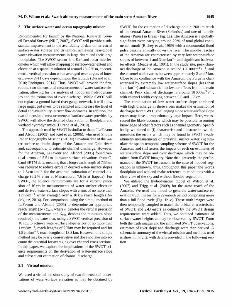
We utilised the hydrodynamic model of Wilson et al.

(2007) and Trigg et al. (2009) for the same reach of the

Amazon. We used this model to generate water-surface el-

evation truth images for a 22-month period comprising more

than a full flood cycle (Fig. 1b–c). These truth images were

then temporally sampled to match the orbital characteristics

of SWOT, and 2-D errors as defined by the SWOT design

requirements were added. Thus, we obtained estimates of

surface-water heights as may be observed by SWOT. From

both the truth images and the simulated SWOT observations,

estimates of river slope and discharge were then derived. A

schematic summary of the virtual mission and methods used

is shown in Fig. 2, with details provided in the following sec-

tion.

www.hydrol-earth-syst-sci.net/19/1943/2015/ Hydrol. Earth Syst. Sci., 19, 1943–1959, 2015


J J A S O N D J F M A M J J A S O N D J F M A2

4

6

8

10

12x 104

Month

Cha

nnel

dis

char

ge, m

3s−1


0.5

1

1.5

2x 104

Month

Cha

nnel

dis

char

ge, m

3s−1

60°45'0"W61°0'0"W61°15'0"W61°30'0"W61°45'0"W62°0'0"W62°15'0"W62°30'0"W62°45'0"W

3°30'0"S

3°45'0"S

4°0'0"S

Solimõ

es

Purus

Bathymetry25 m

-25 m

Topography50 m

0m

0 10 20 30 40 505

km

(a)

(b) (c)

(d)

!Manaus

50°W55°W60°W65°W70°W

0°

5°SAruma

ItapeuaBrazil

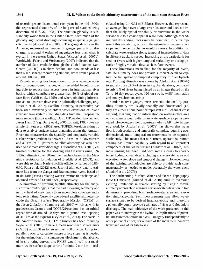
Figure 1. Study area: (a) location of site in the central Amazon, Brazil; (b) Solimões and (c) Purus inflow hydrographs; and (d) SRTM

elevation fused with river bathymetry used in the hydraulic model.

1D water surface

elevations

1D water surface slope

S[MODEL]

Gen

erat

ion

of “v

irtua

l re

ality

”

LISFLOOD-FP, 1D diffusive wave

Mapping to 100 m grid

Inverse Fourier transform of SWOT design error requirements

Spatio-temporal sampling of model output to SWOT

SWOT observation images, h[SWOT OBS]

SWOT “truth”

1D channel discharge Q[MODEL]

Gen

erat

ion

of S

WO

T ob

serv

atio

ns

Estimation of slope using reach-length averaging

S [SWOT OBS]

Cross-sectional averaging

S [SWOT XS] S [TRUE] 1D water

surface slopes

Cal

cula

tion

of sl

ope

and

disc

harg

e

Q [SWOT OBS] Q [SWOT XS] Q [TRUE]

Estimation of channel discharge

1D channel discharges

Width, w Depth, y Friction, n

images h[TRUE]

Figure 2. Schematic diagram of the methods used in this paper.

3 Methods

3.1 Generation of water-surface truth images from

hydrodynamic modelling

In order to generate water elevation truth images, the hy-

drodynamic model code LISFLOOD-FP (Bates and De Roo,

2000) was used. LISFLOOD-FP consists of a 1-D represen-

tation of the river channel which is comprised of a series

of channel cross sections and a 2-D floodplain representa-

tion. The formulation of LISFLOOD-FP used here was the

one-dimensional diffusive wave formulation of Trigg et al.

(2009) for channel flow (floodplain flow was excluded), al-

lowing complex channel bathymetry and back propagation of

flow. A detailed series of rectangular channel cross sections

were used (124 for the Solimões and 48 for the Purus), with

an average along-channel spacing of 2.4 km and each repre-

senting the average bed elevation for that location. Channel

flow was implemented in the form:

∂Q

∂x+∂A

∂t= q, (1)

S0−n2P 4/3Q2

A10/3−

[∂y

∂x

]= 0, (2)

where Q is the volumetric flow rate in the channel, A the

cross-sectional area of the flow, P is the wetted perimeter

(approximated by channel width), n is the Manning friction

coefficient, S0 is the channel bed slope, q is the lateral flow

into and out of the channel, y is the channel depth, x is the



distance along the river and t is time (Trigg et al., 2009).

Note that S0 is written so that it is greater than zero in the

usual case where the bed elevation decreases in the down-

stream direction. The diffusion term,[∂y/∂x

], allows chan-

nel flow to respond to both the channel bed slope and the

water-surface slope. This diffusive wave approximation of

the full 1-D Saint Venant equations is solved using an im-

plicit Newton–Raphson scheme.

In order to create truth images of water-surface elevation

(h[TRUE]), 1-D channel water elevations were first mapped

onto channel cross sections perpendicular to the channel cen-

terline. Across each cross section, the elevation value of the

channel centre was maintained; however, where two or more

cross sections coincided (within 100 m), the arithmetic mean

of each was used. The resulting set of cross sections were

then interpolated onto a 2-D regular grid using a nearest-

neighbour method at a spatial resolution of 100 m. This was

selected to approximately match the design requirements of

SWOT as specified by Rodríguez (2014), although resolu-

tion will vary across the swath. While this method excluded

potential minor cross-channel variation in water-surface el-

evation, variation along channel was incorporated fully, in-

cluding any backwater effects.

Upstream boundary conditions (channel discharge) for the

Solimões (Fig. 1b) and Purus (Fig. 1c) were derived from

rating curves and river stage measurements at in situ gauges

at Itapeua and Aruma (Fig. 1a), respectively, using data pro-

vided by the Agência Nacional de Águas (ANA), Brazil, for

the period 1 June 1995 to 31 March 1997. River stage mea-

sured at Manacapuru was used as the downstream bound-

ary condition. The model developed allowed the inclusion

of a detailed river bathymetry (Fig. 1d), obtained in a field

survey by Wilson et al. (2007) and described in detail by

Trigg et al. (2009). In the study reach, the Solimões varies

in width from around 1.6–5.6 km, with minimum bed eleva-

tion between −26.5 and 8.0 m (vertical datum: EGM96); the

width of the Purus varies from 0.6 to 1.7 km, with minimum

bed elevation between −9.8 and 9.5 m. Friction parameters

for the model were obtained through a calibration based on

the minimisation of RMSE calculated from river levels from

four gauging stations internal to the model domain and model

water-surface elevation obtained at a temporal resolution of

12 h (Trigg et al., 2009).

3.2 Obtaining SWOT observations

Water-surface elevations obtained from LISFLOOD-FP were

used as truth onto which SWOT sampling and errors could be

added, thereby allowing us to assess their hydraulic implica-

tions. Water surfaces were obtained from the model accord-

ing to the SWOT spatio-temporal sampling scheme from an

orbit with 78◦ inclination, 22-day repeat, 97 km altitude, and

140 km swath width. The reach length was sufficient to be

covered by six swaths in total in each 22-day cycle (three

ascending, three descending), with each ground location be-

60°45'0"W61°0'0"W61°15'0"W61°30'0"W61°45'0"W62°0'0"W62°15'0"W62°30'0"W

3°15'0"S

3°30'0"S

3°45'0"S

4°0'0"S

4°15'0"S

Number of observations

2 3

OP 2 (2.39)OP 6 (21.23)

OP 4 (18.30)

OP 1 (0.90)OP 5 (19.79) OP 3 (16.81)

(a)

(b)

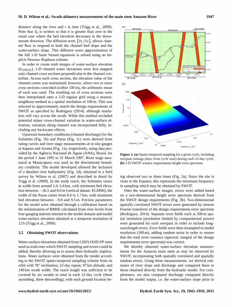
Figure 3. (a) Spatio-temporal sampling for a given cycle, including

overpass timings (days from cycle start) during each 22-day cycle;

(b) 2-D SWOT science requirements height error spectrum.

ing observed two or three times (Fig. 3a). Since the site is

close to the Equator, this represents the minimum frequency

in sampling which may be obtained by SWOT.

Onto the water-surface images, errors were added based

on a two-dimensional height error spectrum derived from

the SWOT design requirements (Fig. 3b). Two-dimensional

spatially correlated SWOT errors were generated by inverse

Fourier transform of the design requirements error spectrum

(Rodríguez, 2014). Separate error fields each at 500 m spa-

tial resolution (resolution limited by computational power)

were generated for each overpass in order to include long-

wavelength errors. Error fields were then resampled to model

resolution (100 m), adding random noise in order to ensure

that the total error variance (spectral, integral of the design

requirements error spectrum) was correct.

We thereby obtained water-surface elevation measure-

ments for the Amazon main stem as may be observed by

SWOT, incorporating both spatially correlated and spatially

random errors. Using these measurements, we derived esti-

mates of river slope and discharge and compared them to

those obtained directly from the hydraulic model. For com-

pleteness, we also compared discharge computed directly

from the model output, i.e. the water-surface slope prior to



adding slope errors. This allowed us to characterise the er-

ror in water-surface slope and discharge estimates from both

the SWOT spatio-temporal sampling scheme and from the

instrument measurement error.

3.3 Calculation of slope and discharge from

water-surface elevations

Initially, single-pixel SWOT water-surface elevation mea-

surements (h[SWOTOBS]) were extracted along the chan-

nel centerline and used to calculate water-surface slope

(S[SWOTOBS]). Note that the water-surface slope is mathemat-

ically equal to the sum of the bed slope (S0) and downstream

changes in water depth[∂y/∂x

]:

S = S0−∂y

∂x. (3)

S was derived by along-reach averaging through the fitting

of 1-D polynomials using least-square estimation to moving

windows placed on the surface-water heights:

S =−

∑xh− kxh∑x2− kx2

, (4)

where k is the number of data points included in the mov-

ing window and x is the distance of the water elevation ob-

servation, h, along the channel; the negative sign constrains

the slopes to be greater than zero in the usual case when h

is decreasing in the downstream direction. The size of the

moving windows used ranged from 0.5 up to 20 km, with

larger windows leading to greater along-channel smoothing

of the data. This process was then repeated using cross-

sectional averages of SWOT water elevation measurements

(h[SWOTXS]), extracted by taking the arithmetic mean of pix-

els across channel in a direction perpendicular to the channel

centerline. Note that, while this may effectively reduce the

random errors present, due to the inclusion of spatially corre-

lated errors in the SWOT water elevations, this process may

not necessarily lead to an improved estimate of discharge.

S[SWOTXS] was calculated from h[SWOTXS] in the same way

as S[SWOTOBS]. For comparison and to assess accuracy of de-

rived estimates ofQ, true slope (S[TRUE]) was also calculated

using water-surface elevation truth images (h[TRUE]) using

Eq. (4).

For each water-surface slope (S[SWOTOBS], S[SWOTXS],

S[TRUE]) at each reach length, discharge along the length of

the channel was derived, following the method of LeFavour

and Alsdorf (2005):

Q=1

nwy5/3S1/2, (5)

where w is the reach-averaged channel width, y is the reach-

averaged river depth and S is the overall water-surface slope.

In this paper, we assume that channel friction, width, and bed

elevation are known. Thus, the focus here is on the impact

of errors in observations of water-surface elevation and the

derived estimates of water-surface slope on the estimation of

discharge. Errors in Q were approximated using first-order

error propagation, via a Taylor series expansion:

σQ ≈∂Q

∂SσS =

1

2QσS

S. (6)

Note that here we have isolated the uncertainty in Q that de-

rives from S. Hydrographs of discharge over time for given

points on the channel were then extracted, with the tempo-

ral frequency of these determined by the SWOT sampling

scheme. Thus, for most locations on the channel, two values

of Q were available in each 22-day cycle.

3.4 Accuracy assessment of SWOT-derived discharge

In addition to the discharge error approximation (σQ) calcu-

lated in Eq. (6), hydrographs of channel discharge obtained

using along-reach averaging (Q[SWOTOBS]) and with added

cross-sectional averaging (Q[SWOTXS]) were directly com-

pared to hydrographs obtained using the true water-surface

elevation (Q[TRUE]). RMSE was calculated for each hydro-

graph using

RMSE=

√√√√∑Tt=1

(Qt

[TRUE]−Qt[PRED]

)2

T, (7)

where Qt[TRUE] is the observed channel discharge derived

from true water-surface elevations at time t , Qt[PRED] is

channel discharge derived from SWOT observations (either

Q[SWOTOBS] or Q[SWOTXS]), and T is the number of data in

the time series. RMSE was then expressed as a percentage of

mean Q[TRUE]:

CV[RMSE] = RMSE ·(Q[TRUE]

)−1. (8)

Finally, the Nash–Sutcliffe model efficiency coefficient

(Nash and Sutcliffe, 1970) was calculated using:

E = 1−

∑Tt=1

(Qt

[TRUE]−Qt[PRED]

)2

∑Tt=1

(Qt

[TRUE]−Qt[TRUE]

)2, (9)

where values of E range between −∞ and 1.0, with 1.0 in-

dicating a perfect match between Q[TRUE] and Q[PRED], and

values less than zero indicating that the mean of Q[TRUE]

is a better predictor of true channel discharge than Q[PRED]

(Legates and McCabe, 1999). Generally, values of E be-

tween 0.0 and 1.0 are considered as acceptable levels of per-

formance (Moriasi et al., 2007).

4 Results and discussion

4.1 Model output and generation of SWOT images

The LISFLOOD-FP model was run for the full 22-month pe-

riod between 1 June 1995 and 31 March 1997, taking around



Table 1. Summary of along-channel variability in modelled water-

surface slope and channel discharge at low and high water.

Variable Water Minimum Maximum Mean Standard

level deviation

So

lim

ões Slope Low 0.15 9.57 1.37 1.53

(cm km−1) High 0.69 7.43 2.19 0.95

Discharge Low 19 765 32 068 26 346 2137.9

(m3 s−1) High 69 918 116 030 99 783 9372.3

Pu

rus

Slope Low −0.12 4.99 0.5 1.02

(cm km−1) High 0.17 3.01 0.52 0.35

Discharge Low −2649 5314 958 1276.4

(m3 s−1) High 6665 19 276 13 466 2958.9

82 h to complete on a dual-processor compute server. The

Manning’s friction coefficient, n, used was 0.032 for the

Solimões and 0.034 for the Purus, obtained from model cal-

ibration by Trigg et al. (2009). The overall RMSE of the

model ranged between 0.1 and 0.9 m (please see Trigg et al.,

2009, for details). Model validation consisted of a compari-

son of model water levels with an independent set of satel-

lite altimetry data, with RMSE found to be 1.26 and 1.42 m

for the Solimões and Purus rivers, respectively (Trigg et al.,

2009).

One-dimensional channel profiles outputs from the

LISFLOOD-FP model are shown in Fig. 4 for low water (15

September 1995) and high water (21 June 1996), including

the water-surface elevation, water-surface slope and channel

discharge, and are summarised in Table 1. There was sub-

stantial along-channel variation in water-surface slope and

channel discharge for the both the Solimões and the Purus at

low and high water. This along-channel variability may make

the accurate estimation of discharge using reach-averaged es-

timates of slope a considerably greater challenge.

Figure 5 indicates water elevation at the upstream and

downstream ends of the Solimões and Purus reaches and av-

erage water-surface slopes throughout the 22-month simula-

tion period. Generally, water-surface slope is lowest during

the falling limb of the hydrograph and highest during the ris-

ing limb. Average water-surface slope for the Solimões rose

quickly to its maximum level of 2.9 cm km−1 during the low

water period (September to November, 1995), immediately

after the river level at the upstream end of the channel started

to rise. The maximum water-surface slope in the Purus of

1.29 cm km−1 occurred during the low water period (Octo-

ber, 1995), when backwater effects from the main Solimões

channel were less important.

As detailed in Sect. 3.2, truth images of water-surface el-

evation, h[TRUE], were generated from LISFLOOD-FP ac-

cording to the SWOT spatio-temporal sampling scheme and

2-D errors were then added to these according to the 2-

D SWOT science requirements height error spectrum, pro-

viding SWOT images of water-surface height observations,

h[SWOTOBS]. Over the 22-month simulation period, there

were a total of 29 orbit cycles (of 22 days each and including

six overpasses of the domain; see Fig. 3a) providing, in total,

174 images of h[SWOTOBS]. An example set of six overpasses

from a SWOT orbit cycle at high water (cycle 18) is shown in

Fig. 6, illustrating the extent of the channel which may be ob-

served. Note that here we are focused on the main channels

and have not attempted to map water elevations in the flood-

plain forest. A detailed inset image of the Purus/ Solimões

confluence for cycle 18, overpass 6 is shown in Fig. 7, illus-

trating the image of h[SWOTOBS] alongside the corresponding

image of h[TRUE] and 2-D SWOT height errors.

Values of SWOT water-surface height observations were

extracted from images of h[SWOTOBS] along the channel cen-

terline and, in addition, averages of channel cross sections

taken perpendicular to the channel centerline were calculated

(h[SWOTXS]), plotted against distance downstream for high

water (cycle 18) in Fig. 8. In these profiles, the tighter clus-

tering of the cross-sectional averages to the true channel wa-

ter elevation profile indicates that by taking a cross-sectional

average, errors in water-surface height observations were re-

duced (assuming no bias in the estimation of water-surface

elevation).

4.2 Water-surface slopes

Figure 9 illustrates along-channel water-surface slope as cal-

culated using h[SWOTXS] for high water (cycle 18, over-

pass 6), using reach lengths between 5 and 20 km. As

the length of averaging increased, errors in S[SWOTXS] re-

duced substantially when compared to S[TRUE]. Overall error

in the estimation of water-surface slope decreased quickly

with increasing reach lengths (Fig. 10): for the Solimões,

without averaging across channel (S[SWOTOBS]) and with a

short reach lengths of 0.5 km, errors in slope were high

at 86.4 cm km−1. These errors dropped quickly as more

data were included in the estimation of slope, reducing to

0.33 cm km−1 at 20 km. Averaging across channel in ad-

dition to along-reach lengths (S[SWOTXS]) led to a further

drop in errors, with 0.09 cm km−1 error at 20 km reach

lengths. Slope errors were similar for the Purus without

cross-sectional averaging (91.0 cm km−1 at 0.5 km; 0.31 at

20 km), and were moderately higher than the Solimões with

cross-sectional averaging (0.13 cm km−1 at 20 km) due to

the narrower channel width (Table 2). The science require-

ment for the SWOT sensor is that river slopes are mea-

sured with errors less than 1 cm km−1 when averaged for

a 10 km reach length (Rodríguez, 2014). As expected from

the methods used, for both the Solimões and Purus, with-

out cross-sectional averaging (S[SWOTOBS]), reach lengths of

∼ 10 km were required to achieve this level of accuracy; with

cross-sectional averaging (S[SWOTXS]), accuracies better than

1 cm km−1 were achieved using shorter reach lengths of ∼ 4

and ∼ 5 km for the Solimões and Purus, respectively. For

10 km reach lengths, incorporating cross-sectional averag-

ing, water-slope errors of 0.26 and 0.37 cm per km, respec-

tively, were achieved.



−20

−10

0

10

20

30E

lev

ati

on

(m

)

0

5

10

Wa

ter

slo

pe

(cm

/km

)

0 50 100 150 200 2500

5

10

x 104

Distance downstream (km)

Ch

an

nel

dis

cha

rge

(m3/s

)

−10

0

10

20

Ele

va

tio

n (

m)

0

1

2

3

4

5

Wa

ter

slo

pe

(cm

/km

)

0 20 40 60 80 100

0

5000

10000

15000

20000


Ch

an

nel

dis

cha

rge

(m3/s

)

(a) (b)Purus inflow to the Solimoes channel

High water

Low water

Figure 4. LISFLOOD-FP model output: 1-D channel profiles at high and low water for (a) the Solimões and (b) Purus rivers. Top: water-

surface elevations along the channel (channel bed topography is shown in grey shaded area); middle: water-surface slope; bottom: channel

discharge. The vertical line in the plots in (a) indicates the location of the Purus inflow to the Solimões.

5

10

15

20

25

Wa

ter

elev

ati

on

(m

)

J J A S O N D J F M A M J J A S O N D J F M A

1

1.5

2

2.5

3

Month

Wate

r sl

op

e (c

m/k

m)

10

15

20

Wa

ter

elev

ati

on

(m

)


0.5

1

Month

Wate

r sl

op

e (c

m/k

m)

(a) (b)

Figure 5. LISFLOOD-FP model output: 1-D channel profiles through time for (a) the Solimões and (b) the Purus rivers. Top plots: water

elevations at the upstream (solid line) and downstream (dashed line) end of the study reach; bottom plots: average water-surface slope through

time.

4.3 Channel discharge

In Fig. 11, along-channel discharge estimates for high wa-

ter (cycle 18, overpass 6) are shown for Q[SWOTXS] us-

ing reach lengths between 5 and 20 km. As with errors in

slope, as reach lengths increased, the errors in estimated dis-

charge decreased. The LISFLOOD-FP modelled discharge

(Q[MODEL]) is also shown for reference. Note thatQ[TRUE] is

different to Q[MODEL] since it does not take into account the

full diffusive wave approximation of the Saint Venant equa-

tions (Sect. 3.1) and is a reach-length average rather than an

instantaneous discharge for a particular location.

Using reach lengths of 20 km, full discharge hydrographs

were constructed for Q[SWOTXS] for several locations along

the Solimões and Purus channels, and are compared to hy-

drographs for Q[TRUE] and Q[MODEL] in Fig. 12. Q[SWOTXS]



Overpass: 1, Day: 374.9

−62.6 −62.2 −61.8 −61.4 −61 −60.6

−4.2

−4

−3.8

−3.6

−3.4


−62.6 −62.2 −61.8 −61.4 −61 −60.6

−4.2

−4

−3.8

−3.6

−3.4


−62.6 −62.2 −61.8 −61.4 −61 −60.6

−4.2

−4

−3.8

−3.6

−3.4


−62.6 −62.2 −61.8 −61.4 −61 −60.6

−4.2

−4

−3.8

−3.6

−3.4


−62.6 −62.2 −61.8 −61.4 −61 −60.6

−4.2

−4

−3.8

−3.6

−3.4


−62.6 −62.2 −61.8 −61.4 −61 −60.6

−4.2

−4

−3.8

−3.6

−3.4

m

18

20

22

24

Figure 6. SWOT water elevation measurements derived from hydraulic model output (Figs. 4 and 5) and science requirements (Fig. 3) for

cycle 18 (at high water), for each of the six overpasses during the 22-day cycle. The box shown in overpass 6 indicates the area shown in

detail in Fig. 7.

0 500 1000 1500 2000 2500 3000 3500 4000

20.5

21

21.5

Distance (m)

Wa

ter e

lev

ati

on

(m

) A B

A

B

−61.56 −61.52 −61.48 −61.44

−3.74

−3.72

−3.7

−3.68

−3.66

−3.64

−3.62

A

B

−61.56 −61.52 −61.48 −61.44

−3.74

−3.72

−3.7

−3.68

−3.66

−3.64

−3.62

m

20.5

21

21.5

(a)

(b)

−61.56 −61.52 −61.48 −61.44

−3.74

−3.72

−3.7

−3.68

−3.66

−3.64

−3.62

σ (m)

−0.5

0

0.5

Figure 7. (a) Detail of 2-D SWOT water-surface elevation for cycle 18, overpass 6 (left) and corresponding “truth” water surface (right) with

added 1 cm contours. Cross sections of water-surface elevation between points A and B are shown for illustrative purposes (h[SWOTOBS]

is the solid red line; h[TRUE] is the dashed grey line). (b) 2-D SWOT errors generated by inverse Fourier transform of the spectrum (see

Fig. 3b).



0 50 100 150 200 250 30018

20

22

24

26Solimoes: Cycle 18, Overpass 1

Wa

ter e

lev

ati

on

(m

)

0 50 100 150 200 250 30018

20

22

24


0 50 100 150 200 250 30018

20

22

24


Wa

ter e

lev

ati

on

(m

)

0 50 100 150 200 250 30018

20

22

24


0 50 100 150 200 250 30018

20

22

24



Wa

ter e

lev

ati

on

(m

)

0 50 100 150 200 250 30018

20

22

24



0 20 40 60 80 10019

20

21

22

23

24Purus: Cycle 18, Overpass 2

0 20 40 60 80 10019

20

21

22

23


0 20 40 60 80 10019

20

21

22

23



SWOT observation, h[SWOT OBS]

SWOT x−section mean, h[SWOT XS]

Model channel profile

Figure 8. The 2-D heights (Fig. 6) were transferred to 1-D for both the Solimões and Purus by extracting values of h[SWOTOBS] along

the channel centerline; to reduce errors, averages of cross sections taken perpendicular to the channel centerline were also calculated

(h[SWOTXS]).

100 120 140 160 180 200 220 240 260

−4

−3

−2

−1

5 km reaches

Wa

ter

slo

pe

(cm

/km

)

100 120 140 160 180 200 220 240 260

−4

−3

−2

−1

10 km reaches

100 120 140 160 180 200 220 240 260

−4

−3

−2

−1

15 km reaches


Wa

ter

slo

pe

(cm

/km

)

100 120 140 160 180 200 220 240 260

−4

−3

−2

−1

20 km reaches


0 20 40 60 80 100−2

−1.5

−1

−0.5

0

0.55 km reaches

Wa

ter

slo

pe

(cm

/km

)

0 20 40 60 80 100−2

−1.5

−1

−0.5

0

0.510 km reaches

0 20 40 60 80 100−2

−1.5

−1

−0.5

0

0.515 km reaches


Wa

ter

slo

pe

(cm

/km

)

0 20 40 60 80 100−2

−1.5

−1

−0.5

0

0.520 km reaches


(a) (b)

Slope, S[SWOT XS]

Slope, S[TRUE]

Figure 9. Slope errors: the effect of averaging along channel using reach lengths between 5 and 20 km for the (a) Solimões and (b) Purus

rivers. Plots show cycle 18 (high water), overpass 6.

matchedQ[TRUE] well throughout the 22-month hydrograph,

including both rising and falling flood wave. As with slope

errors, the error in estimated discharge dropped quickly as

the length of reach-length averaging increased (Fig. 13).

Without averaging water-surface elevations across chan-

nel (Q[SWOTOBS]), errors (CV) were 48.5 % of the mean

Solimões discharge at 5 km reach lengths, reducing to 9.7 %

at 20 km. Averaging across channel in addition to along-

reach lengths (Q[SWOTXS]) led to a further drop in errors,

with 22.2 % error at a reach lengths of 5 km, reducing to

2.6 % at 20 km. Discharge errors for the Purus without cross-

sectional averaging were 130.9% of the mean Purus dis-

charge at 5 km, reducing to 35.1 % at 20 km; conversely, with

cross-sectional averaging errors were 76.0 % at 5 km, reduc-



0 5 10 15 200

1

2

3

4

5

Reach length (km)

Slo

pe

(S)

erro

r, σ

(cm

/km

)

0 5 10 15 200

1

2

3

4

5

Reach length (km)

Slo

pe

(S)

erro

r, σ

(cm

/km

)

(a)

(b)

Science requirements for S

SWOT observation [SWOT OBS]

SWOT x−section mean [SWOT XS]

Figure 10. The effect of reach-length averaging on errors in the

water-surface slope estimation for (a) the Solimões and (b) the Pu-

rus rivers.

ing to 19.1 % at 20 km. Discharge errors are summarised in

Table 2.

Nash–Sutcliffe efficiency coefficient (E) values for with

increasing reach-length averaging are shown in Fig. 13c. On

the Solimões, forQ[SWOTOBS], E was−1.92 at reach lengths

of 5 km, increasing to 0.89 at 20 km; for Q[SWOTXS], E was

0.46 at 5 km, increasing to 0.99 at 20 km. For the Purus, val-

ues of E were lower: for Q[SWOTOBS], E was −8.17 at reach

lengths of 5 km, increasing to 0.57 at 20 km; for Q[SWOTXS],

E was −1.34 at 5 km, increasing to 0.88 at 20 km. Nega-

tive values of E indicate that the prediction of discharge

is no better than the mean value of the observations: con-

sequently, using cross-sectional averaging, reach lengths of

∼ 4 km were required to achieve positive values of E (indi-

cating acceptable levels of accuracy) for the Solimões; for

the Purus, ∼ 7.5 km reach lengths were required. High val-

ues of E (> 0.8) were achieved with reach lengths greater

than ∼ 7.5 km for the Solimões and ∼ 17.5 km for the Purus,

indicating high accuracy in the estimation of discharge.

Table 2. Summary of along-channel variability in modelled water-

surface slope and channel discharge at low and high water.

Error Reach length (km)

So

lim

ões

S[SWOTOBS] σS , cm km−1 2.55 0.91 0.33

S[SWOTXS] σS , cm km−1 0.72 0.26 0.09

Q[SWOTOBS]

RMSE, m3 s−1 34 180 18 900 7190

CV[RMSE], % 48.5 26.1 9.7

E −1.92 0.23 0.89

Q[SWOTXS]

RMSE, m3 s−1 15 670 5950 1960

CV[RMSE], % 22.2 8.3 2.6

E 0.46 0.93 0.99

Pu

rus

S[SWOTOBS] σS , cm km−1 2.57 0.9 0.31

S[SWOTXS] σS , cm km−1 1.05 0.37 0.13

Q[SWOTOBS]

RMSE, m3 s−1 9682 5211 2795

CV[RMSE], % 130.9 67.9 35.1

E −8.17 −0.92 0.57

Q[SWOTXS]

RMSE, m3 s−1 5764 3189 1493

CV[RMSE], % 76 40.9 19.1

E −1.34 0.44 0.88

The above accuracy assessment of SWOT-derived dis-

charge compares estimates obtained using SWOT observa-

tions of water elevation to those obtained using true water-

surface elevations, based on the channel discharge approxi-

mation in Eq. (5), which does not take into account the full

diffusive wave approximation of the Saint Venant equations

shown in (1) and (2). To characterise error introduced by

Eq. (5), Q[TRUE] and Q[SWOT] were also compared using E

to channel discharge obtained directly from LISFLOOD-FP,

using Q[MODEL] in place of Q[TRUE] in Eq. (9) (Fig. 14).

Thus, we were able to characterise errors in estimates of

channel discharge introduced directly by errors in SWOT ob-

servations, as well as errors introduced by the calculation of

Q using reach-length averaging of the water surface in the

calculation of water-surface slope. Errors in Q[TRUE] were

low with a minimum error of 2418 m3 s−1 (3.5 %, E = 0.99)

for the Solimões at a reach length of 0.75 km, and 486 m3 s−1

(6.8 %, E = 0.99) for the Purus at a reach length of 3 km.

However, as the reach length used increased, the errors in

Q[TRUE] also increased. At reach lengths of 20 km, errors

for the Solimões were 5690 m3 s−1 (8.3 %, E = 0.87) and

1238 m3 s−1 (18.1 %, E = 0.89) for the Purus. This increase

in error in conjunction with reach length is primarily a re-

sult of the reach-length averaging used for the calculation of

water-surface slope in Eq. (4), as compared to the instanta-

neous discharge obtained at a single cross section from the

LISFLOOD-FP model output. However, the figures should

be used with caution since errors may also be related to the

structure of the 1-D hydraulic model rather than resulting

from differences with the true channel discharge at a loca-

tion. Notwithstanding this, results illustrate that there may

be an optimal reach length for the estimation of instanta-



100 120 140 160 180 200 220 240 2600.6

0.8

1

1.2

1.4x 10

5 5 km reaches

Dis

cha

rge

(m3/s

)

100 120 140 160 180 200 220 240 2600.6

0.8

1

1.2

1.4x 10

5 10 km reaches

100 120 140 160 180 200 220 240 2600.6

0.8

1

1.2

1.4x 10

5 15 km reaches


Dis

cha

rge

(m3/s

)

100 120 140 160 180 200 220 240 2600.6

0.8

1

1.2

1.4x 10

5 20 km reaches


0 20 40 60 80 100

1

1.5

2

x 104 5 km reaches

Dis

cha

rge

(m3/s

)

0 20 40 60 80 100

1

1.5

2

x 104 10 km reaches

0 20 40 60 80 100

1

1.5

2

x 104 15 km reaches


Dis

cha

rge

(m3/s

)

0 20 40 60 80 100

1

1.5

2

x 104 20 km reaches


(a) (b)

Discharge, Q[SWOT XS]

Discharge, Q[TRUE]

Model discharge, Q[MODEL]

Figure 11. Discharge estimates accounting for slope errors but neglecting width, depth, and friction errors for reach lengths between 5 and

20 km for the (a) Solimões and (b) Purus rivers. Plots show cycle 18 (high water), overpass 6.

0 100 200 300 400 500 6002

4

6

8

10

12x 10

4 Solimoes, distance: 50 km

Dis

cha

rge

(m3/s

)

0 100 200 300 400 500 6002

4

6

8

10

12x 10


0 100 200 300 400 500 6002

4

6

8

10

12x 10


0 100 200 300 400 500 6002

4

6

8

10

12x 10


Dis

cha

rge

(m3/s

)

Time (days)

0 100 200 300 400 500 6002

4

6

8

10

12x 10


Time (days)

0 100 200 300 400 500 6000

0.5

1

1.5

2

x 104 Purus, distance: 50 km

Time (days)

Discharge, Q[SWOT XS]

Discharge, Q[TRUE]

Model discharge, Q[MODEL]

Figure 12. Reconstruction of channel discharge hydrographs from cross-section-averaged SWOT observations (Q[SWOTXS]) for the

Solimões and Purus channels using 20 km reach lengths, compared to discharge obtained using water elevation “truth” images (Q[TRUE])

and the original modelled channel discharge (Q[MODEL]).



0 2 4 6 8 10 12 14 16 18 2010

3

104

105

106

Dis

charg

e (Q

) er

ror,

σ (

m3/s

)

0 2 4 6 8 10 12 14 16 18 200

20

40

60

80

100

Dis

charg

e (Q

) er

ror

(%)

0 2 4 6 8 10 12 14 16 18 20−1

−0.5

0

0.5

1

Nash

−S

utc

liff

e ef

fici

ency

, E

0 2 4 6 8 10 12 14 16 18 2010

3

104

105

Reach length (km)

Dis

charg

e (Q

) er

ror,

σ (

m3/s

)

0 2 4 6 8 10 12 14 16 18 200

20

40

60

80

100

Reach length (km)

Dis

charg

e (Q

) er

ror

(%)

0 2 4 6 8 10 12 14 16 18 20−1

−0.5

0

0.5

1

Reach length (km)

Nash

−S

utc

liff

e ef

fici

ency

, E

(a) (b) (c)



Figure 13. Errors in discharge (Q) as related to reach-length averaging, calculated against slope and discharge obtained using water elevation

“truth” images (Q[TRUE]): (a) absolute discharge error; (b) error expressed as a percentage of mean discharge; and (c) Nash–Sutcliffe

efficiency coefficient. The horizontal line in (c) represents the level of “acceptable” error in modelled discharge estimates. Top row: Solimões;

bottom row: Purus.

neous discharge, beyond which further averaging will lead

to reductions in the accuracy of estimated discharge. For

the Solimões, using cross-sectional averaging (Q[SWOTXS]),

maximum accuracy occurred using reach lengths of 12.5 km

(6258 m3 s−1 error, 9.1 %, E = 0.89), beyond which accu-

racy decreased slightly. For comparison, at this reach length,

errors in Q[TRUE] were 4.7 %, indicating that around 4.4 %

of the error was contributed from SWOT height errors with

the remainder resulting from the method used to calculate

discharge.

4.4 Implications for SWOT

These results indicate that discharge may be obtained accu-

rately from SWOT measurements on large, lowland rivers,

assuming sufficient knowledge of channel bathymetry and

frictional properties. The error in discharge of 2.6 % for the

Solimões using cross-channel averaging and 20 km reach

lengths compares favourably with the error of ∼ 6–8 % ob-

tained by LeFavour and Alsdorf (2005) for the same section

of river using SRTM data and 733 km reach lengths. When

comparing against instantaneous discharge obtained directly

from model output, errors were moderately higher with ac-

curacies of 9.1 % obtained at reach lengths of 12.5 km. This

suggests that SWOT data will provide both an improvement

in accuracy of discharge estimates and a substantial increase

in the level of along-channel detail. Since SWOT will pro-

vide 2-D measurements of surface water, we were able to use

cross-channel averaging to substantially improve accuracy

due to the improved representation of channel water-surface

elevations and subsequent reductions in water-surface slope

errors. For the Purus, accuracy in discharge estimates was

lower, which is likely to have been in large part due to the nar-

rower width of the river leading to a reduction in averaging of

height errors and consequently higher slope errors, combined

with the very low water-surface slopes on the river leading to

a proportionately higher impact of slope errors when calcu-

lating discharge.

The results presented here may be extended to other large

rivers which may be observable by SWOT via Eq. (6). In

Fig. 15, the percentage error in calculated discharge, Q, re-

sulting from errors in SWOT-derived water-surface slope are

indicated for selected rivers, with approximate widths and

water-surface slopes obtained from published sources. These

errors were derived from Eq. (6) using 5 km reach lengths

to estimate water-surface slope, incorporating the effects of

cross-channel averaging of water-surface elevation and as-

suming that the full width of the channel is observable.

As channel width increases, error in discharge decreases

since greater averaging of water-surface elevation is possi-

ble (water-surface elevation errors will decrease by 1/√n,

where n is the number of pixels being averaged Rodríguez,

2014); as water-surface slope decreases, error in discharge

increases since water-surface slope errors become propor-

tionately more important according to Eq. (6). From this, we

can infer that discharge estimates may be more accurate for



0 2 4 6 8 10 12 14 16 18 2010

3

104

105

106

Dis

charg

e (Q

) er

ror,

σ (

m3/s

)

0 2 4 6 8 10 12 14 16 18 200

20

40

60

80

100

Dic

harg

e (Q

) er

ror

(%)

0 2 4 6 8 10 12 14 16 18 20−1

−0.5

0

0.5

1

Nash

−S

utc

liff

e ef

fici

ency

, E

0 2 4 6 8 10 12 14 16 18 2010

2

103

104

105

Reach length (km)

Dis

charg

e (Q

) er

ror,

σ (

m3/s

)

0 2 4 6 8 10 12 14 16 18 200

20

40

60

80

100

Reach length (km)

Dic

harg

e (Q

) er

ror

(%)

0 2 4 6 8 10 12 14 16 18 20−1

−0.5

0

0.5

1

Reach length (km)

Nash

−S

utc

liff

e ef

fici

ency

, E

(a) (b) (c)

Truth image discharge [TRUE]



Figure 14. Errors in discharge (Q) calculated against model discharge (Q[MODEL]): (a) absolute discharge error; (b) error expressed as a

percentage of mean discharge; and (c) Nash–Sutcliffe efficiency coefficient. Top row: Solimões; bottom row: Purus.

rivers with (i) larger channel widths which permit a greater

level of cross-sectional averaging and the use of shorter reach

lengths and (ii) higher water-surface slopes, since the relative

error in discharge decreases as slope increases. Conversely,

discharge estimation accuracy is likely to be the lowest for

narrow (<∼ 1 km width) rivers with low slopes, although fur-

ther research is required to quantify errors for rivers at this

scale. As indicated by the results presented in Fig. 13, longer

reach lengths may lead to reduced error, at the expense of

increasing along-channel approximation.

It is important to note that the errors presented here only

represent the contribution to overall error in reach-averaged

discharge which may be added by SWOT observations of

water-surface elevation. Other errors are excluded but may

be significant and further research is required to charac-

terise their contribution (e.g. errors contributed by friction

or bathymetry, or resulting from along-channel variability in

discharge). Other than surface-water slope and elevation, pa-

rameters required in the estimation of discharge (i.e. chan-

nel width, roughness and bed elevation, or channel depth)

are the subject of other recent studies. For example, Durand

et al. (2008) used data assimilation of synthetic SWOT mea-

surements in a hydraulic model to estimate river bathymet-

ric slope and depth for the same river reach as presented

in this paper, obtaining RMSE of 0.3 cm km−1 and 0.56 m,

respectively. Similarly, Yoon et al. (2012) estimated river

bathymetry for the Ohio River, USA, obtaining an RMSE

of 0.52 m and an effective reach-averaged river roughness

within 1 % of the true value. Finally, Durand et al. (2014)

illustrated the use of a Bayesian algorithm to estimate river

bathymetry and roughness based on observations of river h

and S with high accuracy for the River Severn, UK, and the

subsequent estimation of channel discharge. When compared

to gauge estimates of discharge, Durand et al. (2014) ob-

tained an accuracy of 10 % in discharge estimation for in-

bank flows, assuming known lateral inflows, decreasing to

36 % without this assumption. The work presented in this pa-

per builds on these studies in that it is the first to directly as-

sess the implications of errors in surface-water slope derived

from SWOT observations of water elevation on the estima-

tion of discharge, independent of other factors.

As with other studies, the error analysis presented here ex-

cluded layover and vegetation effects, as may be found in

wetlands and floodplains, or along the edges of rivers. These

effects are likely to be greatest for narrower rivers with bank

vegetation. In addition, research presented here did not in-

corporate effects of the temporal sampling scheme on the ac-

curacy of hydrograph estimation. For large rivers with dis-

charge which changes relatively slowly, such as the Ama-

zon and its sub-basins, errors introduced by SWOT tempo-

ral sampling are likely to be minimal. However, for smaller

rivers with higher discharge variability, this sampling may be

significant. Further research is required in this area, although

it is likely that there will be an optimum level of width, slope,

and discharge variability for discharge estimation.



1

1

1

2

2

2

2

3

3

3

3

3

4

4

4

4

5

5

5

5

15

15

15

10

10

10

20

20

20

30

30

30

50

50

50

100

100

100

Solimoes

Purus

Missouri

Brahmaputra

Niger

Mekong

lower Amazon

Parana

Water surface slope (cm/km)

Riv

er w

idth

(m

)

2 4 6 8 10 12 14 16 18 20 22

103

104

Figure 15. Examples of global rivers which may be observable by SWOT. Contours represent the percentage error in reach-averaged dis-

charge (Q), calculated according to Eq. (6), contributed by errors in water-surface slope derived from SWOT observations, when using 5 km

reach lengths and cross-channel averaging. Errors may be reduced by using longer reach lengths; note that other sources of error are excluded

but may be significant: without full assessment of each river, figures should be used with caution. Sources used to obtain values of river width

and water-surface slopes were the Solimões and Purus rivers (Brazil) from this paper; lower Amazon River (Brazil) from Meade et al. (1985);

Brahmaptura River (India) from Jung et al. (2010); Mekong River (Thailand/ Laos) from Birkinshaw et al. (2012); Missouri River (USA)

from Bjerklie et al. (2005); Niger River (Mali) from Neal et al. (2012); and Paraná River (Argentina) from Depetris and Gaiero (1998).

5 Conclusions

In this paper, we used a virtual mission study of two-

dimensional water-surface elevations which may be obtained

by SWOT for a reach of the central Amazon River in Brazil

and investigated the implications of errors in such measure-

ments on the estimation of water-surface slope and channel

discharge. The following remarks can be made following our

work:

1. Using 1-D polynomials with least-squares estimation

fitted to water elevations obtained from channel center-

lines, the SWOT design requirement of slope errors less

than 1 cm per km when averaged for 10 km (Rodríguez,

2014) was achieved for both the Solimões and Purus

Rivers.

2. Shorter reach lengths (∼ 4 and ∼ 5 km for the Solimões

and Purus, respectively) were required to achieve the

design level of accuracy when additionally averaging

SWOT water-surface height estimates across-channel;

for 10 km reach lengths, higher accuracies were

achieved (water-slope errors of 0.26 and 0.37 cm km−1

for the Solimões and Purus, respectively). This indicates

that the accuracy of water-surface slopes estimates will

be higher for rivers with wider channels, particularly

those several times wider than the ∼ 70–250 m nomi-

nal spatial resolution (Durand et al., 2010; Rodríguez,

2014).

3. SWOT data are promising for the estimation of Amazo-

nian river discharge, with low errors in estimates (9.1 %

for instantaneous estimates, or 2.6 % for reach-averaged

discharge estimates). Discharge hydrographs could be

reconstructed accurately from SWOT imagery based on

the specified temporal sampling scheme (Figure 3; Ro-

dríguez, 2014) although, for rivers with a higher dis-

charge variability, temporal sampling is likely to be a

significant source of error for hydrograph estimation.

4. A high proportion of the errors found in the instanta-

neous estimates derived from the method used to cal-

culate discharge from water-surface slopes, rather than

from SWOT errors, suggesting that improvements to the

estimation of discharge may be possible.

It should be noted that the errors added to water surfaces to

simulate SWOT measurements of water elevation were spa-

tially correlated at multiple scales (according to the SWOT

design requirements error spectrum and incorporating long-

wavelength errors for each orbit), with added random noise

on a per-pixel basis. While averaging along cross sections

will effectively reduce the random noise component (assum-

ing no bias), it was not immediately apparent how spatially

correlated error would affect the estimation of discharge.

Results here indicate that, at this scale, these errors do not

greatly impact discharge accuracy – although similar assess-

ments of other rivers is needed.



Overall, these findings indicate that forthcoming SWOT

imagery shows considerable promise for the hydraulic char-

acterisation of large rivers such as the Amazon, although fur-

ther work is required for a range of additional rivers with a

variety of characteristics, particularly those with a high spa-

tial and temporal variability in surface-water slope and chan-

nel discharge.

A final note of caution: in this paper, we assumed knowl-

edge of channel friction, width, and bed elevation in the cal-

culation of discharge, since our aim was to characterise the

impact of SWOT observations and their associated errors

independently of these issues. We also excluded the poten-

tial effects of vegetation on errors in SWOT surface water

heights. Further work is needed to assess the relative impor-

tance of each of these factors on the estimation of channel

discharge.

Acknowledgements. This research was completed while M. D. Wil-

son was a visiting researcher at the School of Earth Sciences,

Ohio State University. M. Durand is supported by a NASA SWOT

Science Definition Team Grant (no. NNX13AD96G). The authors

would like to thank R. Romanowicz and one anonymous referee for

their careful reviews and valuable recommendations which have

improved the quality of this manuscript.

Edited by: R. Moussa

References

Alsdorf, D., Lettenmaier, D., and Vörösmarty, C.: The Need for

Global, Satellite-based Observations of Terrestrial Surface Wa-

ters, Eos, Transactions American Geophysical Union, 84, 269–

275, doi:10.1029/2003EO290001, 2003.

Alsdorf, D., Bates, P., Melack, J., Wilson, M., and Dunne,

T.: Spatial and temporal complexity of the Amazon flood

measured from space, Geophys. Res. Lett., 34, L08402,

doi:10.1029/2007GL029447, 2007a.

Alsdorf, D., Rodríguez, E., and Lettenmaier, D.: Measuring

surface water from space, Rev. Geophys., 45, RG2002,

doi:10.1029/2006RG000197, 2007b.

Bates, P. and De Roo, A.: A simple raster-based model for flood in-

undation simulation, J. Hydrol., 236, 54–77, doi:10.1016/S0022-

1694(00)00278-X, 2000.

Berry, P. A. M., Garlick, J. D., Freeman, J., and Mathers, E.: Global

inland water monitoring from multi-mission altimetry, Geophys.

Res. Lett., 32, L16401, doi:10.1029/2005GL022814, 2005.

Birkett, C.: Contribution of the TOPEX NASA Radar Altimeter to

the global monitoring of large rivers and wetlands, Water Resour.

Res., 34, 1223–1239, doi:10.1029/98WR00124, 1998.

Birkett, C., Mertes, L., Dunne, T., Costa, M., and Jasinski,

M.: Surface water dynamics in the Amazon Basin: Applica-

tion of satellite radar altimetry, J. Geophys. Res., 107, 8059,

doi:10.1029/2001JD000609, 2002.

Birkinshaw, S. J., Moore, P., Kilsby, C., O’Donnell, G. M., Hardy,

A., and Berry, P. A. M.: Daily discharge estimation at ungauged

river sites using remote sensing, Hydrol. Process., 28, 1043–

1054, doi:10.1002/hyp.9647, 2012.

Bjerklie, D., Lawrencedingman, S., Vorosmarty, C., Bolster, C., and

Congalton, R.: Evaluating the potential for measuring river dis-

charge from space, J. Hydrol., 278, 17–38, doi:10.1016/S0022-

1694(03)00129-X, 2003.

Bjerklie, D. M., Moller, D., Smith, L. C., and Dingman,

S. L.: Estimating discharge in rivers using remotely

sensed hydraulic information, J. Hydrol., 309, 191–209,

doi:10.1016/j.jhydrol.2004.11.022, 2005.

Depetris, P. J. and Gaiero, D. M.: Water-surface slope, total sus-

pended sediment and particulate organic carbon variability in the

Parana River during extreme flooding, Naturwissenschaften, 85,

26–28, doi:10.1007/s001140050445, 1998.

Durand, M., Andreadis, K. M., Alsdorf, D. E., Lettenmaier,

D. P., Moller, D., and Wilson, M.: Estimation of bathymet-

ric depth and slope from data assimilation of swath altimetry

into a hydrodynamic model, Geophys. Res. Lett., 35, L20401,

doi:10.1029/2008GL034150, 2008.

Durand, M., Fu, L.-L., Lettenmaier, D., Alsdorf, D., Rodríguez,

E., and Esteban-Fernandez, D.: The Surface Water and Ocean

Topography Mission: Observing Terrestrial Surface Water

and Oceanic Submesoscale Eddies, P. IEEE, 98, 766–779,

doi:10.1109/JPROC.2010.2043031, 2010.

Durand, M., Neal, J., Rodríguez, E., Andreadis, K. M., Smith,

L. C., and Yoon, Y.: Estimating reach-averaged discharge

for the River Severn from measurements of river wa-

ter surface elevation and slope, J. Hydrol., 511, 92–104,

doi:10.1016/j.jhydrol.2013.12.050, 2014.

Fekete, B. M. and Vörösmarty, C.: The current status of global river

discharge monitoring and potential new technologies comple-

menting traditional discharge measurements, in: Predictions in

Ungauged Basins: PUB Kick-off (Proceedings of the PUB Kick-

off meeting held in Brasilia, 20–22 November 2002). IAHS Publ.

309, November 2002, 129–136, IAHS, Wallingford, UK, 2007.

Hossain, F., Katiyar, N., Hong, Y., and Wolf, A.: The emerging

role of satellite rainfall data in improving the hydro-political sit-

uation of flood monitoring in the under-developed regions of

the world, Nat. Hazards, 43, 199–210, doi:10.1007/s11069-006-

9094-x, 2007.

Jung, H. C., Hamski, J., Durand, M., Alsdorf, D., Hossain, F., Lee,

H., Hossain, A. K. M. A., Hasan, K., Khan, A. S., and Hoque,

A. Z.: Characterization of complex fluvial systems using remote

sensing of spatial and temporal water level variations in the Ama-

zon, Congo, and Brahmaputra Rivers, Earth Surf. Process. Land.,

35, 294–304, doi:10.1002/esp.1914, 2010.

Kiel, B., Alsdorf, D., and Lefavour, G.: Capability of SRTM C- and

X-band DEM Data to Measure Water Elevations in Ohio and the

Amazon, Photogramm. Eng. Rem. S., 72, 1–8, 2006.

Lambin, J., Morrow, R., Fu, L.-L., Willis, J. K., Bonekamp, H.,

Lillibridge, J., Perbos, J., Zaouche, G., Vaze, P., Bannoura, W.,

Parisot, F., Thouvenot, E., Coutin-Faye, S., Lindstrom, E., and

Mignogno, M.: The OSTM/Jason-2 Mission, Mar. Geod., 33, 4–

25, doi:10.1080/01490419.2010.491030, 2010.

LeFavour, G. and Alsdorf, D.: Water slope and discharge in the

Amazon River estimated using the shuttle radar topography mis-

sion digital elevation model, Geophys. Res. Lett., 32, L17404,

doi:10.1029/2005GL023836, 2005.


http://dx.doi.org/10.1029/2003EO290001

http://dx.doi.org/10.1029/2007GL029447

http://dx.doi.org/10.1029/2006RG000197

http://dx.doi.org/10.1016/S0022-1694(00)00278-X

http://dx.doi.org/10.1016/S0022-1694(00)00278-X

http://dx.doi.org/10.1029/2005GL022814

http://dx.doi.org/10.1029/98WR00124

http://dx.doi.org/10.1029/2001JD000609

http://dx.doi.org/10.1002/hyp.9647

http://dx.doi.org/10.1016/S0022-1694(03)00129-X

http://dx.doi.org/10.1016/S0022-1694(03)00129-X

http://dx.doi.org/10.1016/j.jhydrol.2004.11.022

http://dx.doi.org/10.1007/s001140050445

http://dx.doi.org/10.1029/2008GL034150

http://dx.doi.org/10.1109/JPROC.2010.2043031


http://dx.doi.org/10.1007/s11069-006-9094-x

http://dx.doi.org/10.1007/s11069-006-9094-x

http://dx.doi.org/10.1002/esp.1914

http://dx.doi.org/10.1080/01490419.2010.491030

http://dx.doi.org/10.1029/2005GL023836


Legates, D. R. and McCabe, G. J.: Evaluating the use

of “goodness-of-fit” Measures in hydrologic and hydrocli-

matic model validation, Water Resour. Res., 35, 233–241,

doi:10.1029/1998WR900018, 1999.

Meade, R. H., Dunne, T., Richey, J. E., DE M Santos, U., and

Salati, E.: Storage and remobilization of suspended sediment

in the lower Amazon river of Brazil, Science, 228, 488–90,

doi:10.1126/science.228.4698.488, 1985.

Meade, R. H., Rayol, J. M., Conceicão, S. C., and Natividade, J.

R. G.: Backwater effects in the Amazon River basin of Brazil,

Environ. Geol. Water S., 18, 105–114, doi:10.1007/BF01704664,

1991.

Moriasi, D. N., Arnold, J. G., Van Liew, M. W., Bingner, R. L.,

Harmel, R. D., and Veith, T. L.: Model Evaluation Guidelines

for Systematic Quantification of Accuracy in Watershed Simula-

tions, T. ASABE, 50, 885–900, doi:10.13031/2013.23153, 2007.

Nash, J. and Sutcliffe, J.: River flow forecasting through conceptual

models part I – A discussion of principles, J. Hydrol., 10, 282–

290, doi:10.1016/0022-1694(70)90255-6, 1970.

Neal, J., Schumann, G., and Bates, P.: A subgrid channel model

for simulating river hydraulics and floodplain inundation over

large and data sparse areas, Water Resour. Res., 48, W11506,

doi:10.1029/2012WR012514, 2012.

NRC: Earth science and applications from space: National impera-

tives for the next decade and beyond, National Acadamies Press,

Washington, DC, available at: http://www.nap.edu/catalog.php?

record_id=11820 (last access: 1 August 2014), 2007.

NSTC: Science and technology to support fresh water availability

in the United States, Tech. Rep. November, National Science

and Technology Council, Committee on Environment and Nat-

ural Resources, subcommittee on Water Availability and Quality,

Washington, DC, available at: http://water.usgs.gov/owq/swaq.

pdf, last access: 1 August 2004.

Papa, F., Bala, S. K., Pandey, R. K., Durand, F., Gopalakrishna,

V. V., Rahman, A., and Rossow, W. B.: Ganga-Brahmaputra river

discharge from Jason-2 radar altimetry: An update to the long-

term satellite-derived estimates of continental freshwater forc-

ing flux into the Bay of Bengal, J. Geophys. Res., 117, C11021,

doi:10.1029/2012JC008158, 2012.

Richey, J. E., Nobre, C., and Deser, C.: Amazon river discharge and

climate variability: 1903 to 1985, Science (New York, N.Y.), 246,

101–103, doi:10.1126/science.246.4926.101, 1989.

Rodríguez, E.: Surface Water and Ocean Topography Mission

(SWOT): Science Requirements Document, Tech. rep., NASA

Jet Propulsion Laboritory, available at: http://swot.jpl.nasa.gov/

files/swot/SWOT_Science_Requirements_Document.pdf, last

access: 1 August 2014.

Seyler, F., Calmant, S., Silva, J. S. D., Moreira, D. M., Mercier,

F., and Shum, C.: From TOPEX/Poseidon to Jason-2/OSTM

in the Amazon basin, Adv. Space Res., 51, 1542–1550,

doi:10.1016/j.asr.2012.11.002, 2013.

Shiklomanov, A. I., Lammers, R., and Vörösmarty, C.: Widespread

decline in hydrological monitoring threatens Pan-Arctic re-

search, Eos, Transactions American Geophysical Union, 83, 13–

17, doi:10.1029/2002EO000008, 2002.

Trigg, M., Wilson, M. D., Bates, P. D., Horritt, M. S., Alsdorf, D. E.,

Forsberg, B. R., and Vega, M. C.: Amazon flood wave hydraulics,

J. Hydrol., 374, 92–105, doi:10.1016/j.jhydrol.2009.06.004,

2009.

USGS: A New Evaluation of the USGS Streamgaging Network: A

Report to Congress, Tech. rep., United States Geological Survey,

available at: http://water.usgs.gov/streamgaging/report.pdf (last

access: 1 August 2014), 1998.

Vorosmarty, C., Askew, A., Grabs, W., Barry, R. G., Birkett, C.,

Doll, P., Goodison, B., Hall, A., Jenne, R., Kitaev, L., Landwehr,

J., Keeler, M., Leavesley, G., Schaake, J., Strzepek, K., Sun-

darvel, S. S., Takeuchi, K., and Webster, F.: Global water data:

A newly endangered species, Eos, Transactions American Geo-

physical Union, 82, 54–54, doi:10.1029/01EO00031, 2001.

Wilson, M., Bates, P., Alsdorf, D., Forsberg, B., Horritt, M.,

Melack, J., Frappart, F., and Famiglietti, J.: Modeling large-scale

inundation of Amazonian seasonally flooded wetlands, Geophys.

Res. Lett., 34, L15404, doi:10.1029/2007GL030156, 2007.

Wolf, A. T., Natharius, J. A., Danielson, J. J., Ward, B. S., and Pen-

der, J. K.: International River Basins of the World, Int. J. Water

Resour. D., 15, 387–427, doi:10.1080/07900629948682, 1999.

Yoon, Y., Durand, M., Merry, C. J., Clark, E. a., Andreadis, K. M.,

and Alsdorf, D. E.: Estimating river bathymetry from data assim-

ilation of synthetic SWOT measurements, J. Hydrol., 464–465,

363–375, doi:10.1016/j.jhydrol.2012.07.028, 2012.


http://dx.doi.org/10.1029/1998WR900018

http://dx.doi.org/10.1126/science.228.4698.488

http://dx.doi.org/10.1007/BF01704664

http://dx.doi.org/10.13031/2013.23153

http://dx.doi.org/10.1016/0022-1694(70)90255-6

http://dx.doi.org/10.1029/2012WR012514

http://www.nap.edu/catalog.php?record_id=11820

http://www.nap.edu/catalog.php?record_id=11820

http://water.usgs.gov/owq/swaq.pdf

http://water.usgs.gov/owq/swaq.pdf

http://dx.doi.org/10.1029/2012JC008158

http://dx.doi.org/10.1126/science.246.4926.101

http://swot.jpl.nasa.gov/files/swot/SWOT_Science_Requirements_Document.pdf

http://swot.jpl.nasa.gov/files/swot/SWOT_Science_Requirements_Document.pdf

http://dx.doi.org/10.1016/j.asr.2012.11.002

http://dx.doi.org/10.1029/2002EO000008


http://water.usgs.gov/streamgaging/report.pdf

http://dx.doi.org/10.1029/01EO00031

http://dx.doi.org/10.1029/2007GL030156

http://dx.doi.org/10.1080/07900629948682


swath-altimetry measurements of the main stem amazon … · 1944 m. d. wilson et al.:...

Documents