Sustainability with Unbalanced Growth: The Role of Structural Change

Ramón E. López, Gustavo Anríquez, and Sumeet Gulati #

April 16, 2003 Working Paper Number: 2003-02

Food and Resource Economics, University of British Columbia Vancouver, Canada, V6T 1Z4 http://www.agsci.ubc.ca/fre

# Ramón E. López and Gustavo Anríquez are at the University of Maryland at College Park, Sumeet Gulati is at the University of British Columbia. Please address all correspondence to Gustavo Anríquez, 2200 Symons Hall, University of Maryland, College Park, Maryland, 20742, USA, phone: (301) 405-1293, fax: (301) 314-9091, email: ganrique@arec.umd.edu

brought to you by COREView metadata, citation and similar papers at core.ac.uk

provided by Research Papers in Economics

1

Sustainability with Unbalanced Growth: The Role of Structural Change

I. Introduction

Are growth and environmental sustainability compatible? At least since Malthus (Essay on the

Principle of Population (1798)) economists have studied the relationship between growth and natural

resources. Recently a sizeable literature studying sustained growth in the presence of natural

resources or pollution has developed. This literature builds on current neoclassical growth theory,

and is almost entirely based on models with a single final good. In such models, the growth of

income and environmental damages derive from the same sector. As we explain below, this restricts

the options available for environmentally sustainable growth.

In a model with a single final good, sustained and environmentally sustainable growth is

possible only after making special assumptions. Smulders and Gradus (1996) provide restrictions on

production and pollution abatement technologies that make growth environmentally sustainable.

Their restrictions are, a unitary elasticity of substitution between pollution and physical capital in

production, and a greater than unitary elasticity of pollution reduction from abatement expenditures.

In other words, abatement expenditures are relatively more effective in reducing pollution than

increases in pollution from growth. Assuming the existence of certain types of externalities can also

generate environmentally sustainable growth. For example, using the Ak model of endogenous

growth, Huang and Cai (1994) rely on the externality effects of government spending on pollution

control to generate sustainable growth1. Schou (2000) meanwhile emphasizes human capital

externalities for sustainable growth.

1 Their explanation for long-term growth is a government spending externality on pollution control. With an exogenously given tax rate, government expenditure on pollution control increases in the same proportion as growth in output. This causes pollution to grow slower than the growth in output and utility continues to grow in the equilibrium growth path.

2

Also using an Ak model of endogenous growth, Stokey (1998) has to depend on exogenous

technical change to achieve sustained and environmentally sustainable growth. She finds that

growth and preservation of the environment are possible only if exogenous technical change allows

growth in output at lower pollution intensities. 2 Aghion and Howitt (1998) extend the Stokey

(1998) model to endogenize technical change and demonstrate that sustainable growth is possible

without exogenous technical change, or exogenously imposed externalities. However, they

summarize their model of renewable natural resources in the following words, “it appears that

unlimited growth can indeed be sustained, but it is not guaranteed by the usual sorts of assumptions

that are made in endogenous growth theory” (p. 162).3 4 Aghion and Howitt (1998) are concerned

with the assumption that the elasticity of marginal rate of consumption is greater than one (or that

utility is highly concave). This assumption is also necessary for sustainable growth in Stokey (1998).

In a model with homothetic preferences it ensures that individuals are willing to make the required

sacrifices in consumption needed for sustainability.

In this paper we present a model with two final good sectors and three productive assets.

Using this model we show that sustainable growth is possible without exogenous technical change,

exogenously imposed externalities, or assumptions that are considered unusual, or restrictive in the

literature. This is possible due to the inclusion of two final good sectors: ‘clean’ (all non-polluting

industries and services) and ‘dirty’. The three assets in the model are: natural capital (a renewable

resource specific to the ‘dirty’ sector), physical or financial capital (specific to the ‘clean’ sector) and

human capital (used in both sectors). Investment is possible in all three assets. As the economy

2 Stokey (1998) uses a simple one-sector model (Ak model), with one input, and negative utility effects of pollution. 3 Their assumptions are: the elasticity of marginal utility of consumption should be greater than one, the research technology should be productive, and the growth rates brought about by the above two assumptions should not be too high so as to cause unmanageable environmental damage. 4 One could characterize this literature as grappling with the tradeoff between economic growth and a clean environment. Another way to achieve sustainable growth would be to completely reject this tradeoff. Bovenberg and

3

grows it imposes increasing demands on natural capital. This threatens the survival of natural capital

and the feasibility of economic growth. Thus, the model possesses the standard tradeoff between

growth and sustainability. However, it offers a novel rationale for sustainable growth, that is,

investment in natural capital combined with endogenous changes in the sectoral composition of

output (commonly termed structural change5).

Chenery (1960) and Kuznets (1957) present structural change (both across countries and

over time) as a stylized fact of the modern growth process. Baumol (1967) and Baumol et al. (1985)

hypothesize differences in the rate of technical change across sectors as the main cause for structural

change. More recently, Echevarria (1998), Laitner (2000) and Kongsamut et al. (2001) highlight the

non-homotheticity of preferences as a causal factor. In this paper we show that structural change

can arise from supply considerations even if preferences are homothetic and technical change is

identical across sectors. Structural change helps to make long-run economic growth compatible

with natural resource sustainability.6 Along the growth path, a relative contraction of the natural

resource using (or damaging) sector is optimal to reduce the costs of preserving natural capital.

Endogenous changes in the share of the dirty good are brought about by unbalanced growth in

assets. Along the growth path, physical, and human capital grow at non-constant rates different

from each other.

This growth path is perhaps the most striking result from this paper. If the marginal

regeneration of natural capital (nature’s intrinsic productivity) is less than the marginal productivity

of man made capital (human or physical capital) a reduction in the share of the dirty good becomes

optimal. As the share of the dirty good contracts, the share of labor income to total income declines

Smulders (1995) and (1996) do exactly that. They postulate that technological progress is driven by stricter environmental regulation. Under this assumption they show that environmentally sustainable growth is possible. 5 Structural change refers to a reduction of output and employment shares of the primary (mostly natural resource intensive production like mining, forestry etc.) sector during the growth process.

4

and the physical capital to output ratio rises. Meanwhile, the stock of natural capital, and the growth

rates for welfare, and income remain constant. We also show that the divergence of asset and

sectoral growth from a balanced path (where all sectors and assets grow at the same rate) is higher

for poorer countries than for richer countries further along in their equilibrium growth path.

The remainder of the paper is structured as follows. In Section II we present the model

used. In Section III we define equilibrium for our model and analyze the properties of equilibrium.

Section III concludes the main body of the paper.

II. The Model

Consider a small open economy with a representative agent consuming two final goods (one ‘clean’

and one ‘dirty’). The production of the clean good (denoted c) has no impact on the environment,

while production of the dirty good (denoted d) harms the environment. The clean good represents

the non-polluting productive sectors of the economy. The dirty good represents all remaining

natural capital intensive (harvesting, or extractive) and/or polluting sectors of the economy.

A benevolent social planner allocates investment in three assets: human capital (h), natural

capital (θ), and physical capital (k). The social planner uses lump sum transfers to finance

investment.

Consumption

The representative consumer consumes two final goods (the clean and the dirty good). Let pc

denote the price of the clean good, and pd the price of the dirty good. Correspondingly let Xc

denote consumption of the clean good and Xd consumption of the dirty good.

Preferences of the representative consumer are defined using an expenditure function.

6 Our attempt is not to undermine the importance of technical progress and preferences in structural change. We only

5

1 2

,( , ) min : ( ) ( )

c d

c d c c d d c d

X XE p p U p X p X X X Uα α α≡ + = . (1)

Parameters 1 2,α α are the standard parameters in a Cobb-Douglas utility function with 01 >α ,

02 >α and 1 2 1α α+ < . This ensures that the utility function is strictly concave. The parameter α

is defined as 1 21/( )α α α≡ + >1.

Consistent with the assumption of a small open economy units are adjusted to ensure that all

goods prices equal 1. This allows us to normalize (1,1) 1E = from equation(1). Therefore the

expenditure function has a simple form, U α .

Production and Labor Market Clearing

The clean sector includes all non-polluting industries and services. Inputs used in its production are

raw labor (Lc), labor augmenting human capital (h ≥ 1), and sector specific physical capital (k). The

production function for the clean good is

( , )c cQ G k hL= . (2)

Where G(⋅) is increasing, concave, and linearly homogenous in k and hLc. G(⋅) also satisfies the

Inada conditions, in other words, as the quantity of an input approaches zero its marginal product

tends to infinity.

Using linear homogeneity of G(.), returns to sector specific physical capital can be denoted

by a restricted profit function

( , / ) max ( , )c

c c c c

Lk p w h p G k hL wLπ = − , (3)

wish to point out another rationale where structural change is optimal.

6

where w is the wage rate for labor. The function π is non-decreasing in pc, non-increasing in w/h,

homogenous of degree one, and jointly convex in (pc, w/h) (Diewert, 1974). Using Hotelling’s

lemma, clean good output equals the derivative of the profit function with respect to price of output

( ( )cpQ kπ= ⋅ , all subscripts denote partial derivatives), and labor employed equals the derivative of

the profit function with respect to the effective wage rate ( /( / ) ( )cw hL k h π= − ⋅ ). Given that all prices

equal 1 the following notation is adopted ( / ) ( 1, / )cw h p w hπ π≡ = .

The dirty sector includes production that is either directly dependent on natural resources or

is highly polluting. Examples are: primary industries such as mining, fishing, forestry, and

agriculture, or highly polluting industrial products. Production of the dirty good uses raw labor (Ld),

labor augmenting human capital (h), and the stock of natural capital (θ) as inputs.

The production function for dirty good is

d dQ hLθ= . (4)

This function corresponds to the standard specification for production based on natural resources.

It was introduced to the literature in a more general form by Gordon (1954) who argued that the law

of diminishing returns was not appropriate for modeling fisheries. The specific form above (from

equation (4)) was later proposed by Schaefer (1957). Since then this specification has been widely

used in modeling natural resources. Recent users include Brander and Taylor (1998 and 1998a),

Conrad (1995), and Munro and Scott (1993).

One unit of dirty good output reduces current stock of natural capital by dφ , with 0 < dφ <

1. If the dirty good is assumed to be a primary or extractive commodity output (from equation (4))

can be written as [ (1- ) ]d d d d dQ hL hLφ φ θ= + , where d dhLφ θ is the harvest of the resource, and

7

(1- )d dhLφ θ is processing. Alternatively, dφ can be interpreted as pollution generated per unit of

output.

The labor market is perfectly competitive. Aggregate labor supply in the economy is fixed at

L . Labor market clearing requires the sum of labor employed in the dirty and clean sectors to equal

the total labor supply, c dL L L+ = . This condition can be re-expressed as

/ ( ) dw h

k L Lhπ− ⋅ + =

Note that there are constant marginal returns to labor in the dirty sector. Also note that there are

diminishing returns to labor in the clean sector. This implies that the dirty good is produced as long

as the aggregate labor supply is large enough. When the dirty good is produced the wage rate equals

the marginal value product of labor in production of the dirty good, formally w= dp hθ . For now,

assume that the dirty good is produced in this economy.7

Asset Accumulation

The social planner allocates investment across all forms of capital. Let jI denote investment in each

of the capital assets , , j h kθ∈ . Growth in labor augmenting human capital is given by

h hh I hδ= − , (5)

where hδ is the rate of depreciation of h. The rate of depreciation of human capital can be

interpreted as the proportion of annual retirements from the workforce. Equation (5) implies that if

investment exceeds depreciation the stock of human capital grows. Any growth in human capital

augments labor input in both sectors (see production functions in equations (2) and (4)). In other

words, growth in human capital equals endogenous labor augmenting technical change.

7 We later prove that specialization in either good is never optimal.

8

Let g(θ) be the intrinsic growth function of the renewable natural resource. The function

has an inverted U shape with ( ) 0gθθ θ < , and (0) ( ) 0g g θ= = , where θ is the ‘carrying capacity’

of the natural resource. The carrying capacity of a natural resource is the maximum stock that can be

sustained in its natural surroundings.8 Let Iθ denote human investment in natural capital, such as:

tree planting, national park protection, fish replenishment including aquaculture investments,

protection of marine ecosystems, soil protection including terracing, drainage, agricultural fallowing

as well as the cleaning-up of ecosystems. Evolution over time of the natural resource stock is

( ) , 0

,

d d

d d

g I hL if

hL if

θθ φ θ θ θθ

φ θ θ θ

+ − ≥ ≥ = − >

. (6)

Growth of the natural resource comprises its natural capacity to regenerate, investment (Iθ),

and the reduction of natural capital from production of the dirty good ( d dhLφ θ ).9 Note that

investment cannot maintain the natural resource beyond its carrying capacity (see equation (6) for

θ θ> ). Investment can substitute for natural regeneration only if the natural resource is within its

natural bounds 0,θ θ∈ . This reflects the fact that a natural resource involves constraints outside

human control. If investment in a natural resource could maintain stock beyond its natural carrying

capacity, the natural resource would be no different from other forms of man-made capital.

The stock of physical capital k grows according to the following equation.

k kk I kδ= − , (7)

8 If there is no extraction, the stock of natural resource stabilizes at its carrying capacity (see Conrad (1995) for examples of such a growth function). 9 Note that in equation (6), the clean sector does not cause any damage to natural capital. However, one could allow the clean sector output to cause environmental damages as well. As long as the clean sector causes less damage than the extractive sector such a change would not alter the results presented.

9

where kδ is the rate of depreciation of k. Equation (7) implies that if investment in physical capital

exceeds depreciation, its stock grows.

The Social Planner’s Problem

The social planner maximizes the present value of utility for the representative consumer by

optimally investing in human, natural and physical capital. Let ρ denote the social discount rate.

The social planner’s maximization problem is

, , ,

0

max ( )exph k

t

U I I IV U t dt

θ

ρ∞

−≡ ∫ (8)

where t denotes time. Maximization of utility is subject to the following set of constraints: all capital

growth equations ((5)-(7)), initial conditions for capital stocks, (for human capital 00(0)h h= where

h(t) is the stock of human capital at time t, for natural capital 00(0)θ θ= , and for physical capital

00(0)k k= ), non negativity constraints U(t) ≥ 0, Ih(t) ≥ 0, Iθ(t) ≥ 0, and Ik(t) ≥ 0, and the following

budget constraint,

( )h kU I I I hL kα θ θ π θ+ + + ≤ + . (9)

The budget constraint requires that total consumption and total investment expenditures should be

no greater than society’s total income. Recall that the wage rate w = θh when the dirty good is

produced. This implies that the first term on the right-hand-side of equation (9), hLθ , equals the

total wage bill for this economy. Due to the same reason return to owners of clean capital can be

represented as kπ (θ).

10

Let λ be the Lagrangean multiplier associated with the budget constraint, and µ, η and Ω be

the co-state variables associated with human, natural, and physical capital respectively. The solution

to the problem in equation (8) is found by maximizing a continuous time current value Hamiltonian.

( )

( ) ( )

h k h h

d k k

U k hL U I I I I h

g I hL k I k

α θ

θθ

λ π θ θ µ δ

η θ φ θ π θ δ

Η = + + − − − − + − + + − + +Ω −

, (10)

where H is defined under the assumption that the natural resource is within its natural bounds

( )0,θ θ∈ (see the discussion of Proposition 1 below for the case where θ θ= ).

III. Equilibrium

Definition 1. The economy is said to be in equilibrium at time t if ˆt t∀ ≥ , µ η λ= = Ω = .

Equilibrium requires that the current value shadow price of the three assets and the shadow

price of current income (consumption) be equal to each other. The social planner invests in an asset

only if its current value is at least as great as the value of current consumption. Further,

simultaneous investment in all three assets is possible only when their current values coincide. If the

three current values are not equal to each other, investment is optimal only in the asset with the

greatest marginal product. In this case the most valuable asset grows faster than the rest leading to a

relatively quicker decline in its current value. Recursive use of the same logic implies that the

current value of all three assets can equalize in the long run (see Proposition 1 below for the

necessary and sufficient conditions for this equilibrium). 10

10 We call it equilibrium because of the difference with what is commonly called a steady state. Originally, steady state referred to stagnation (Solow (1956)). However, as models evolved to allow for growth in equilibrium the concept of steady state evolved to the state where both asset(s) and the economy grew at the same and constant rate (see for example, Cass (1965) and Koopmans (1965) for the single asset case, and Lucas (1988) with two assets). As we illustrate later, in the equilibrium we present, assets grow at different and varying rates, but welfare grows at a constant rate. If the reader is willing to narrow the concept of steady state to a condition where the welfare grows at a constant rate, then the equilibrium presented can also be labeled ‘steady state’.

11

Using the definition of equilibrium and the expressions for co-state variable dynamics

derived from the Hamiltonian (equation (10)), we obtain a trajectory for the current value of h.

(1 )h d Lµ ρ δ φ θµ= + − − . (11)

Optimal utilization of human capital implies that its current value rises at the rate of social discount

( ρ ). The current value of human capital also increases as depreciation ( hδ ) reduces its stock. The

final term on the right hand side of equation (11) is the marginal addition to income from human

capital net of damages to natural capital. The current value of human capital is the discounted sum

of all future income streams. As the marginal income net of environmental damage from human

capital: (1 )d Lφ θ− is expended, the current value of human capital declines.

From the Hamiltonian, trajectories for the current value of natural and physical capital can

also be obtained. The trajectory for the current value of natural capital is given by

[ ( )] [ ] d dkg h L L khθ θ θ θθ

η ρ φ π π φ θπη

= − − − + − − . (12)

The current value of natural capital rises at the rate of social discount. It also rises or falls depending

on the intrinsic marginal productivity (termed marginal regeneration from now on) of natural capital

( gθ ). The current value of natural capital also declines as marginal income net of environmental

damage ( [ ]d dh L Lφ− ) is expended.11 The final term on the right hand side of equation (12)

( [( ]dk θ θθπ φ θπ− ) is the effect of increasing natural capital on the clean sector. An increase in

natural capital implies an increase in the wage rate for labor (recall wage is θh). This reduces profits

in the clean sector due to an increase in the wage bill ( k θπ ). The increase in wages causes a

12

reduction in employment in the clean sector and the retrenched labor is employed in the dirty sector

causing a reduction in natural capital. This effect is captured by the term d k θθφ θ π− .

The trajectory for the shadow value of physical capital is given by

[ [ ]]k dθρ δ π φ θ πΩ

= + − + −Ω

. (13)

The current value of physical capital rises at the rate of social discount. It also decreases as marginal

income net of environmental damage of physical capital ( [ ]dθπ φ θ π+ − ) is spent. Note that an

increase in physical capital reduces damages to the environment ( [ ] 0dθφ θ π− > ). An additional unit

of physical capital raises production of the clean good. This raises income in society (π ) and draws

labor away from the dirty sector. This increase in employment eases pressure on the stock of natural

capital (reflected in the term [ ]dθφ θ π in equation (13)). Besides generating income, accumulation of

physical capital has a positive environmental effect by drawing labor away from otherwise extractive

or polluting uses.

From definition 1, equilibrium requires that the current value shadow price of the three

assets and the shadow price of current income (consumption) be equal to each other

(µ η λ= = Ω = ).12 This implies that the rates of growth for the current value shadow prices also

coincide ( / / / /µ µ η η λ λ= = Ω Ω = ).

If we equate equation (11) and (13) (i.e., / /µ µ = Ω Ω ) we obtain

[ ] (1 )d k d hLθπ φ θ π δ φ θ δ + − − = − − . (14)

11 ( / ) dL k h Lθπ+ = , i.e., the damages to natural capital from an increase in natural capital are d dhLφ .

12 The first order conditions for maximization of H in (10) and µ η λ= = Ω = imply 0, 0hI I θ> > and 0kI > .

13

Equation (14) imposes equality between the net marginal products of physical and human capital.

The left hand side is the net marginal product of physical capital. It includes an increase in physical capital

income (π ) and the net gain to the natural resource from an expansion of clean production

( [ ]dθφ θ π− ). The right hand side is the net marginal product of human capital. It includes the marginal

increase in wages net of damages to natural capital, and depreciation. Equation (14) solves for an

equilibrium solution for the stock of natural capital *( )θ . That is, the definition of equilibrium used

implies that the stock of natural capital achieves a stationary level, i.e., that the economy in

equilibrium reaches environmental sustainability. Investment in θ will exactly off-set the net use of

the natural capital so that 0θ = .

The next step is to determine the economy’s growth rate at the equilibrium stock of natural

capital. Using / /λ λ µ µ= , we obtain

* *1( ) (1 )1

d hU LU

ω θ φ θ δ ρα

≡ = − − − −, (15)

where natural capital is evaluated at its equilibrium value θ*. Equation (15) is an expression for

utility growth along equilibrium. It shows that utility growth is constant along equilibrium.

Conditions for Equilibrium

Thus far we show that the economy may achieve permanent positive welfare growth while keeping

the natural capital stock stationary. The following proposition establishes the conditions necessary

for such an equilibrium.

Proposition 1. If a) *(1 )d hLφ θ δ ρ− − > , and b) [ ]hd L δθφα

ρ −−> *)1(1 and c) *θ θ≤ , then

equilibrium (as defined in Definition 1) exists and this equilibrium allows for diversified sustainable

development.

14

The equilibrium illustrates ‘diversified sustainable development’. Equilibrium is diversified if

there is production of both the clean and the dirty good. Sustainable development is defined as a

condition where the stock of natural capital remains stationary, while welfare grows. Three

conditions are necessary for a diversified sustainable equilibrium. The bracketed term in the right

hand side of equation (15) is the difference between the marginal product of human capital and the

social discount rate. Condition a) requires that this difference be positive for positive growth.

However, if the growth in welfare *( )ω θ is too large the social planner’s objective function in

equation (8) becomes unbounded. Condition b) ensures that the social planners objective function

is bounded. It is a re-expression of the condition *( )ρ ω θ> (see Appendix A). Finally the

equilibrium stock of natural capital should be less than the carrying capacity of the environment

(condition c)). Conditions a), b) and c) are necessary and sufficient for the equilibrium in Definition 1

(see proof in appendix A). Specialization in any sector is not consistent with equilibrium. An

equality of shadow values requires that the economy invest in all three assets. Since k and θ are

sector specific factors investment in both sectors implies that both sectors must be productive.

Conditions a) and b) are simultaneously feasible when 1>α . This assumption only requires

the utility function to be strictly concave. No further restrictions on the elasticity of marginal utility

of consumption are needed for equilibrium. In contrast, some earlier models of sustainable growth

required the elasticity of marginal utility of consumption to be greater than one (a stronger

requirement than strict concavity). This required the marginal utility of consumption to decline

rapidly along the growth path to ensure that the sacrifices in consumption needed to make growth

sustainable were carried out.

Growth in this model is sustainable not only due to the sacrifices made in consumption

(rising investment in natural capital) but also due to endogenous changes in structure of the

15

economy. As in earlier models greater investment in natural capital is needed as the economy grows,

however besides sacrifices in consumption an endogenous change in the structural composition of

output economizes on the consumable resources needed for investment along the growth path. We

discuss the endogenous change in structure in greater detail later in the paper.

When condition c) is not satisfied specialization in the clean sector becomes optimal (see

Appendix A for a formal proof) and the economy does not value natural capital. This justifies our

definition of equilibrium. Equilibrium according to Definition 1 allows us to study meaningful

sustainable development in a context where natural capital is socially valuable (please see Appendix

B for an exposition of condition c) in the context of a Cobb-Douglass production function for the

clean good).

Figure 1 shows the level of natural capital (θ*) where net marginal products for human and

physical capital are equalized. The net marginal product for physical capital decreases as natural

capital increases. The net marginal product for human capital increases at a constant rate as natural

capital increases. This ensures a unique intersection where both net marginal products are equal. If

at the point of intersection the net marginal product of man-made assets (human and physical

capital) is higher than the rate of discount (as shown in figure 1) equilibrium is characterized by

positive welfare growth. However if at this intersection, man-made assets are less productive than

the discount rate, growth is not feasible. In this case, the economy is characterized by implosion.

16

Figure 1. The net marginal products of k and h and the level of θ, the case of a growing economy

Optimal Growth Rates of Man-Made Assets with Stationary Natural Capital

Since θ* is constant along equilibrium the growth rate of natural capital equals zero. From equation

(6) this implies that the sum of investment and intrinsic growth of natural capital is equal to the

damage to the resource, formally

* *( ) d dI g hLθ θ φ θ+ = . (16)

Sustainable development is in part possible due to investment in natural capital. However damage

to natural capital, and its intrinsic growth rate (see equation (16)) also influence the growth rate for

natural capital. The intrinsic growth rate depends solely on the stock of natural capital. Equilibrium

growth paths for human and physical capital determine how damage to natural capital grows along

gθ

MP*

*θ

MPk

MPh

MP

θ

ρ

17

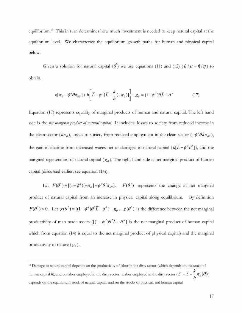
equilibrium.13 This in turn determines how much investment is needed to keep natural capital at the

equilibrium level. We characterize the equilibrium growth paths for human and physical capital

below.

Given a solution for natural capital (θ*) we use equations (11) and (12) ( / /µ µ η η= ) to

obtain.

[ ] [ ( )] (1 )d d d hkk h L L g Lhθ θθ θ θπ φ θπ φ π φ θ δ − + − − − + = − −

(17)

Equation (17) represents equality of marginal products of human and natural capital. The left hand

side is the net marginal product of natural capital. It includes: losses to society from reduced income in

the clean sector ( k θπ ), losses to society from reduced employment in the clean sector ( d k θθφ θ π− ),

the gain in income from increased wages net of damages to natural capital ( [ ]d dh L Lφ− ), and the

marginal regeneration of natural capital ( gθ ). The right hand side is net marginal product of human

capital (discussed earlier, see equation (14)).

Let * *( ) [(1 )[ ] ]d dF θ θθθ φ π φ θ π≡ − − + . *( )F θ represents the change in net marginal

product of natural capital from an increase in physical capital along equilibrium. By definition

*( ) 0F θ > . Let * *( ) [(1 ) ]d hL gθχ θ φ θ δ≡ − − − . *( )χ θ is the difference between the net marginal

productivity of man made assets ( *[(1 ) ]d hLφ θ δ− − is the net marginal product of human capital

which from equation (14) is equal to the net marginal product of physical capital) and the marginal

productivity of nature ( gθ ).

13 Damage to natural capital depends on the productivity of labor in the dirty sector (which depends on the stock of

human capital h), and on labor employed in the dirty sector. Labor employed in the dirty sector ( ( )dL Lkh θπ θ= + )

depends on the equilibrium stock of natural capital, and on the stocks of physical, and human capital.

18

When *( ) 0χ θ < the net marginal productivity of man-made assets is less than the marginal

productivity of nature. When 0χ ≥ the net marginal productivity of man-made assets is greater

than the marginal productivity of nature. In figure 1 at equilibrium (intersection of marginal

products of human and physical capital) the marginal productivity of nature is lower than the

marginal productivity of human and physical capital. In other words figure 1 illustrates the case

where *( ) 0χ θ > .

At equilibrium with a constant stock of natural capital (θ*) equation (17) represents a

relationship between human and physical capital. Using the two terms ( )F θ , and ( )χ θ , equation

(17) is expressed as

* *(1 ) ( ) ( )d hL F kφ θ χ θ− − = . (18)

Equation (18) implies that *( ) /[(1 ) ]dh k F Lθ φ = − . Note that (1 ) 0d Lφ− > is the

marginal change in the net marginal product of natural capital from an increase in human capital (see

equation (17)). As both ( )F θ and (1 )d Lφ− are positive, human and physical capital grow or

decline together in equilibrium. Equation (18) also implies that human and physical capital need not

grow at the same rate. The relationship between the rates of change for human and physical capital

is

*( )1

(1 )d

h kh k hL

χ θφ

= − −

. (19)

We characterize this relationship using the following proposition.

Proposition 2. During equilibrium the physical/human capital ratio, k/h, is increasing if and only if χ > 0. That

is, / / 0k k h h ><− iff 0χ >

< .

19

Equation (19) implies that human capital grows slower than physical capital when nature’s

productivity is lower than the productivity of man-made assets, that is ( )* 0χ θ > . We believe this to

be the normal case. In modern societies we expect man-made assets to provide greater marginal

value than the intrinsic growth of natural resources. If either forms of man made capital (physical or

human) have a very low productivity this may not be the case. Note that at equilibrium (from

equation (14)) * * * * *( ) [(1 ) ] ( ) [ ]( )d h d kL g gθ θ θχ θ φ θ δ π θ φ θ π θ δ ≡ − − − + − − = − . Thus a low

marginal product of physical capital will cause *( )π θ to be low and thus can cause ( )*χ θ to be

negative. Similarly, if the economy is sparsely populated the return to human capital is not high

enough (as L is low) and ( )*χ θ can be negative. In such cases the productivity of nature is higher

than the productivity of man-made assets, and human capital grows faster than physical capital.

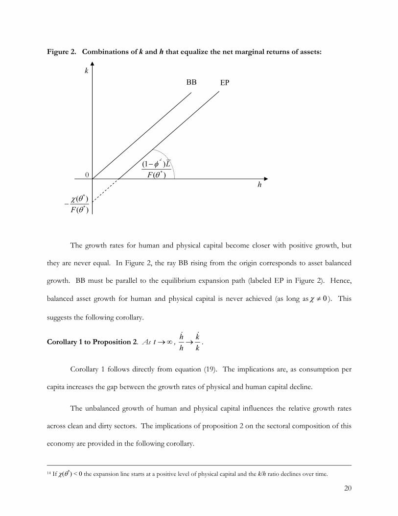
Figure 2 depicts the ‘equilibrium expansion path,’ EP (given by equation(18)). The

‘equilibrium expansion path’ is derived for the equilibrium value of natural capital under the

assumption that the productivity of man-made assets is higher than nature. The equilibrium expansion

path represents combinations of physical and human capital that are needed to maintain the equality

of the net marginal products of all assets. A growing economy in equilibrium must expand physical

and human capital along the equilibrium expansion path maintaining a fixed level of natural capital

(θ*). As illustrated in figure 2 the physical capital to human capital (k/h) ratio permanently increases

along the equilibrium expansion path.14

20

Figure 2. Combinations of k and h that equalize the net marginal returns of assets:

The growth rates for human and physical capital become closer with positive growth, but

they are never equal. In Figure 2, the ray BB rising from the origin corresponds to asset balanced

growth. BB must be parallel to the equilibrium expansion path (labeled EP in Figure 2). Hence,

balanced asset growth for human and physical capital is never achieved (as long as 0χ ≠ ). This

suggests the following corollary.

Corollary 1 to Proposition 2. As t →∞ , h kh k→ .

Corollary 1 follows directly from equation (19). The implications are, as consumption per

capita increases the gap between the growth rates of physical and human capital decline.

The unbalanced growth of human and physical capital influences the relative growth rates

across clean and dirty sectors. The implications of proposition 2 on the sectoral composition of this

economy are provided in the following corollary.

14 If χ(θ*) < 0 the expansion line starts at a positive level of physical capital and the k/h ratio declines over time.

EP

h

k

*

(1 )( )

d

LFφθ

−0

*

*

( )( )F

χ θθ

−

BB

21

Corollary 2 to Proposition 2. Along the equilibrium expansion path, if 0χ > ;(i) The share of labor employed

in the dirty sector declines. (ii) The ratio of value of dirty output to the value of total output declines. (iii) The

share of labor income in total income declines. (iv) The physical capital to output ratio in the economy rises. If

0χ < , the exactly opposite results hold.

Proof: Please see Appendix A.

The social planner uses a combination of instruments to keep natural capital constant (or

equivalently to attain sustainable development). These instruments are investment and a variation in

the structural composition of output. Investment in the replenishment of natural capital acts as

public pollution abatement. Additionally, to economize on the use of consumable resources for

investment, the structural composition of output is altered. When the productivity of nature is high

relative to the productivity of man-made assets, growth in the share of the dirty sector does not

affect the sustainability of natural capital. However when natures intrinsic productivity is low the

dirty sector is shrunk relative to the rest of the economy so as to preserve natural capital. When

natures intrinsic productivity is low it is more costly (in terms of investment in natural capital) to

sustain the equilibrium value of natural capital. This makes it necessary to complement the

investment effort in natural capital with a gradual shift of the structure of production towards the

clean sector. The method of achieving structural change is by allowing physical capital to grow

faster than human capital.

IV. Conclusion

The main contribution of this paper is to show that permanent growth and environmental

sustainability can be compatible even if technical change is completely endogenous. Investment in

the environment combined with an optimal variation in the composition of output ensures

permanent welfare growth without harming the environment.

22

Most studies explaining growth in the presence of natural resources rely on models with a

single final good. They achieve sustained and sustainable growth only after imposing special

conditions. We illustrate that such special conditions are not necessary to achieve environmentally

sustainable growth.

We find that an adjustment in the composition of output (between clean and dirty sectors) is

crucial to economize on the costs of environmental sustainability. This optimal adjustment is

achieved seamlessly due to the presence of a social planner. A useful extension of our research

would be to determine the optimal tax and transfer framework that would bring about this

adjustment in a market framework.

23

References

Aghion, P. and P. Howitt (1998), Endogenous Growth Theory, MIT Press, Cambridge. Baumol, W. J., S. A. B. Blackman, and E. N. Wolff (1985), “Unbalanced Growth Revisited:

Asymptotic Stagnancy and New Evidence,” American Economic Review, 75(4):806-17. Baumol, W. J (1967), “Macroeconomics of Unbalanced Growth: The Anatomy of Urban Crisis,”

American Economic Review, 57(3):415-426. Bovenberg A.L. and S.A. Smulders (1995), “Environmental Quality and Pollution-Augmenting

Technological Change in a Two Sector Endogenous Growth Model,” Journal of Public Economics, 57:369-91.

Bovenberg A.L. and S.A. Smulders (1996), “Transitional Impacts of Environmental Policy in an Endogenous Growth Model,” International Economic Review, 37(4):861-893.

Brander J. and M. Taylor, (1998) “The Simple Economics of Easter Island: A Ricardo-Malthus Model of Renewable Resource Use,” American Economic Review, 88(1): 119-138.

Brander J. and M. Taylor, (1998a) “Open Access Renewable Resources: Trade and Trade Policy in a Two-Country Model,” Journal of International Economics, 44(2):181-209.

Cass, David (1965), “Optimum Growth in an Aggregative Model of Capital Accumulation,” Review of Economic Studies, 32: 233-240.

Chenery, H. B. (1960), “Patterns of Industrial Growth,” American Economic Review, 50:624-654. Clark, Colin (1990), Mathematical Bioeconomics. The Optimal Management of Renewable

Resources, John Wiley and Sons, New York. Conrad, J.M. (1995), “Bioeconomic models of the fishery,” Handbook of Environmental Economics, (D.

Bromley, ed.) Oxford, Blackwell, 405-432 Diewert W. E. (1974), “Applications of Duality Theory,” in Frontiers of Quantitative Economics Vol. II,

edited by M. Intriligator and D. Kendrick, North-Holland, Amsterdam, pp. 106-71. Echevarria, C. (1997), “Changes in Sectoral Composition Associated with Economic Growth,”

International Economic Review, 38(2):431-52. Gordon, H. S. (1954), “The Economic Theory of a Common Property Resource: The Fishery,”

Journal of Political Economy, 63(2):124-42. Huang, C. and D. Cai (1994), “Constant-Returns Endogenous Growth with Pollution Control,”

Environmental and Resource Economics, 4(4):383-400. Kongsamut P., S. Rebelo, and D. Xie (2001), “Beyond Balanced Growth”, Review of Economic Studies,

68(4):869-82. Koopmans, Tjalling (1965), “On the Concept of Optimal Economic Growth,” in The Economic

Approach to Development Planning, Amsterdam, North Holland. Kuznets S. (1957), “Quantitative Aspects of the Economic Growth of Nations II,” Economic

Development and Cultural Change, Supplement to Volume V(4):3-11. Laitner, J. (2000) “Structural Change and Economic Growth,” Review of Economic Studies, 67:545-61. Lucas, R. E. (1988), “On the Mechanics of Economic Development,” Journal of Monetary Economics,

22(1): 3-42. Munro G. R. and A. D. Scott (1993), “The economics of Fisheries Management,” in Handbook of

Natural Resource and Energy Economics, Volume III, Kneese and Sweeney eds., North Holland.

24

Schaefer, M.B. (1957), “Some Considerations of Population Dynamics and Economics in Relation to the Management of Marine Fisheries,” in Journal of the Fisheries Research Board of Canada, 14:669-81.

Schou P. (2000), “Polluting Non-Renewable Resources and Growth,” Environmental and Resource Economics, 16(2): 211-27.

Smulders S.A. and R. Gradus (1996), “Pollution Abatement and Long-Term Growth,” European Journal of Political Economy, 12:505-32.

Solow, R. M. (1956), “A Contribution to the Theory of Economic Growth,” Quarterly Journal of Economics, 70(1):65-94.

Stokey N.L. (1998), “Are There Limits to Growth?” International Economic Review, 39(1):1-31. Tahvonen O. and J. Kuuluvainen (1991), “Optimal Growth with Renewable Resources and

Pollution,” European Economic Review, 35:650-61.

25

Appendix A: Proofs

Derivation of Proposition 1 b).

The condition stated in Proposition 1 b) follows from the transversality conditions for man made assets. We begin by noting that by the end of the planning horizon man made assets and all investments grow at approximately the same rate. From equation (5) and (7) if growth rates for assets are finite it is necessary that / /k kk k I I= and

/ /h hh h I I= . Additionally, as t tends to infinity, the difference in the rates of growth of man made assets approaches zero, as can be seen from (19); that is : / /t k k h h→∞ ≈ . Finally, from (16) it can be seen, as θ is fixed, eventually / /h h I Iθ θ= . Differentiating the budget constraint (9) with respect to time we get:

* * *( ) ( )k h

k hk h

h k I I IU hL k I I Ih k I I I

θα θ

θαω θ θ π θ= + − − − . (20)

Given that man made assets and investments tend to grow at the same rate by the end of the planning horizon we have from (20) and (9) that: as : /t k k αω→∞ ≈ . From the first order condition for welfare we have that / ( 1)α ωΩ Ω = − − , where we have used the equilibrium condition that / /λ λ = Ω Ω . We can now simplify the transversality condition for capital Lim ( ) ( ) 0t

te t k tρ−

→∞Ω = , to:

( 1)0Lim 0t t t

te e k eρ α ω αω− − −

∞→∞Ω = , (21)

where 0Ω is the level of the shadow value of assets and income when equilibrium is achieved and k∞ is an arbitrarily large capital level at which the asset grows at its asymptotic rate. The condition expressed in (21) will hold as long as ρ ω> .

Proposition 1 c): Proof of Diversification when *θ θ≤ .

Condition c) from Proposition 1 requires that equilibrium stock of natural capital be less than the carrying capacity of the environment Suppose not, if *θ θ> the equilibrium solution for the natural resource is carrying capacity (a corner solution for θ*). At θ the net marginal product of k is greater than that of h (see Figure 1). The economy invests only in k and not in h. This implies that compared to the dirty sector the marginal product of labor in the clean sector rises. The clean sector grows and absorbs labor. This process leads to specialization in the clean sector.

A diversified equilibrium necessarily occurs if *θ θ≤ . Assume that *θ θ≤ and that the economy specializes in the clean sector. From labor market clearing with specialization

/( / ) (( / ) ) 0c s sw hL L k h w hπ= + = , (22)

26

where the superscript s denotes equilibrium values under specialization. In other words, ( / )sk h is the physical capital to human capital ratio when the economy specializes in the clean sector. Under specialization the net marginal products of k and h (in the clean sector) are equal, thus,

/(( / ) ) (( / ) )s s

s sw h

k ww h w hh h

π π = −

, (23)

where ( )/ sk h and ( / )sw h are the long-run equilibrium values for k/h and w/h under specialization. Combine (22) and (23) to obtain

(( / ) )( / )

s

s

w hLw h

π= . (24)

Compare the solution from (24) with * *( / )w hθ = in the diversified equilibrium. From (14), assuming for simplicity that depreciation rates are equal, diversified equilibrium is given by

* *

* *

*

( )1( ) ( )

1

d

dL

θφ θ π θπ θ π θθ φ

−

=−

, (25)

which is feasible given that *θ θ< . Since 0θπ < and 1dφ < we have that the term in square bracket in (25) is greater than 1. This implies that

*

*

( ) (( / ) )( / )

s

sw h

w hπ θ πθ

< . (26)

Since ( ).π is a decreasing function the inequality in equation (26) can only occur if

( )* / sw hθ > . That is, the wage rate under diversified equilibrium is higher than under specialization in the clean sector. Specialization in the clean sector cannot be sustained. Labor migrates into the primary sector in search of higher wages allowing the primary sector to become productive. As long as *θ θ≤ specialization in the clean sector is not optimal. Specialization in the dirty sector is ruled out by Inada conditions assumed. As 0cL → the marginal product of labor in the industrial sector approaches infinity. The clean sector always attracts workers from the primary sector when the level of employment is sufficiently low.

Proof for Corollary 2 to Proposition 2. Note that from proposition 2 the following holds true: if

0χ >< then / / 0k k h h >

<− . This implies that if 0χ > : (i) *( )d kL Lh θπ θ= + declines along

the growth path. (ii) Using (i) we get that the share of value of dirty output to total value of

output in this model *

* *(1, )

dd

dp

hLshL k

θθ π θ

=+

declines. (iii) The share of labor income in

27

total income is *

* *( )w hLInc

hL kθ

θ π θ=

+ which too declines during the equilibrium growth

path. Finally (iv) the capital output ratio for this economy can be expressed as:

* *(1, )dp

k ky hL kθ π θ=

+ which rises along the equilibrium growth path.

Appendix B: Conditions Necessary for Diversification with Cobb-Douglass Clean Production

To shed additional light on condition c) from Proposition 1 assume a Cobb-Douglas production function for the clean good, 1( )c b c bQ Bk hL −= , where B is total factor productivity in the clean industry, and 0 1b< < is the share of capital in the industry. It is easy to verify that the unit profit function in this case is 1/ (1 ) /( ) [ /(1 )] b b bb b Bπ θ θ − −= − . The solution to equation (14) in this case (assuming for simplicity that h kδ δ= ) is

1/* (1 )(1 )bdb L Bθ φ

−

= − − . Condition c) from Proposition 1 requires that

1// (1 )(1 )

bdB b Lθ φ γ< − − ≡

Recalling that d dQ hLθ= , we can interpret θ as the maximum level that total factor productivity of man-made assets can reach in the dirty industry. Thus the condition for diversification requires that the total factor productivity of man made assets in the industrial sector to be not much larger than the maximum attainable total factor productivity in the primary sector. If /B θ γ< then the primary or dirty sector is potentially competitive with the industrial sector and eventually diversified equilibrium at *θ θ< is attained. If /B θ γ> then the dirty sector cannot compete and eventually the economy would specialize in the clean sector.