susan m. cormier, ph.d. ncea-cincinnati-u.s. epa · 28-08-2015 · susan m. cormier, ph.d....
TRANSCRIPT
The views expressed in this presentation are those of the author and do not necessarily reflect the policies
of the U.S. Environmental Protection Agency
Susan M. Cormier, Ph.D.NCEA-Cincinnati-U.S. EPA
Invited Expert Meeting on Revising U.S. EPA’s Guidelines forDeriving Aquatic Life Criteria
14-16 September 2015, Arlington, VA

Why conductivity andWhy a new method?
• Biological impairments are known to occur instreams that meet benchmarks derived by thelaboratory method.
• In low conductivity waters, more than 50% ofgenera are affected and streams still meet thelaboratory based benchmarks.
2

Advantage Directly measures actual exposures ofresident organisms and includes direct andindirect effects across entire life cycles
Weakness Exposures and deleterious effects mustalready have done their damage (i.e., datasets for new and rare pollutants areunlikely)Observed effects may be caused ormodified by coincidentally occurring agents(i.e., confounders)
Advantages of Field Method

Theoretical foundation of field-SD aquatic life benchmarks
• Organisms have evolved different physiologiesand behaviors;
• Variation within and among species results indifferent tolerance ranges to both natural andxenobiotic challenges;
• Where a physiological tolerance is exceeded, ataxon is not expected to be present;
• Therefore, upper tolerance levels of many taxacan be used to develop models to predict theproportion of extirpation for a given exposure. 4

Unimodal
5Specific conductivity (µS/cm
Pro
bab
ility
of
Ob
serv
ing
Lirc
eus
Lower UpperOptimum95%
6
Pro
bab
ility
of
Ob
serv
ing
Eph
emer
ella
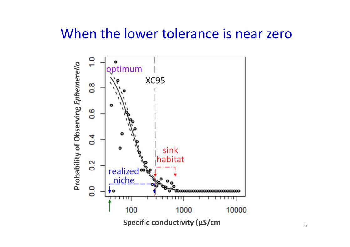
Specific conductivity (µS/cm
When the lower tolerance is near zero

2,210 sampling sites
7

Example of Field-SD Method
• Exposure endpoint: major ions measured asspecific conductivity
• Effect endpoint: extirpation of a taxon,concentration below which 95% of theoccurrences of a genus were observed (XC95)
8

Calculation of XC95
Paired SC and biota data were used toestimate the XC95 of > 100 benthic aquaticinvertebrate genera
9
Drunella
Conductivity ( S/cm)
Cum
ula
tive
Pro
babili
ty
32 100 316 1000
0.0
0.2
0.4
0.6
0.8
1.0
Nigronia
Conductivity ( S/cm)
Cum
ula
tive
Pro
babili
ty
32 100 316 1000 3162 10000
0.0
0.2
0.4
0.6
0.8
1.0

The XC95 values plotted in a genus SDand 5th centile (HC05) identified
10
Conductivity (µS/cm)
Pro
po
rtio
no
fG
en
era
100 200 500 1000 2000
0.0
00
.05
0.1
00
.15
0.2
00
.25
0.3
0
295 µS/cm
Conductivity (µS/cm)
Pro
po
rtio
no
fG
en
era
200 500 1000 2000 5000 10000
0.0
0.2
0.4
0.6
0.8
1.0
295 µS/cm
Specific conductivity (µS/cm
Pro
po
rtio
no
fG
ener
a

Characteristics of Causation
11
• time order
• co-occurrence
• antecedence
• sufficiency
• interaction
• alteration

• time order
• co-occurrence
• preceding causation
• sufficiency
• interaction
• alteration
12
Cause Effect
No measurements before and afterto develop evidence

• time order
• co-occurrence
• preceding causation
• sufficiency
• interaction
• alteration
13
CauseEffect
Conductivity
μS/cm
Ephemeroptera
Present Absent
≤200 852 7
>1,500 50 61
Example: contingency tableWest Virginia Kentucky
Generapresent
Generaabsent
Generapresent
Generaabsent
Near background SC 162 1 104 0
(<150 µS/cm) (99.9) (0.01%) (100%) (0%)
High SC 123 40 58 46
(1,500 µS/cm) (75.5%) (24.5%) (55.8%) (44.2%)

• time order
• co-occurrence
• antecedence
• sufficiency
• interaction
• alteration
14
CauseSource
Samples removed with 0% valley fill(OLS, n=78) r = 0.75

• time order
• co-occurrence
• antecedence
• sufficiency
• interaction
• alteration
15

• time order
• co-occurrence
• antecedence
• Sufficiency
• interaction
• alteration
16
H2O +CO2
CarbonicAnhydrase
HCO3−
H+
Cl− Cl−
a)
Organism’sbody
HCO3−
Na+
Na+
H2O +CO2
CarbonicAnhydrase
HCO3−
H+
Cl−Cl−
HCO3−
Na+
Na+
Stream
b)
Gill epithelium
H2O +CO2
CarbonicAnhydrase
HCO3−
H+
Cl− Cl−
a)
Organism’sbody
HCO3−
Na+
Na+
H2O +CO2
CarbonicAnhydrase
HCO3−
H+
Cl−Cl−
HCO3−
Na+
Na+
Stream
b)
Gill epithelium

• time order
• co-occurrence
• antecedence
• sufficiency
• interaction
• alteration
17

• time order
• co-occurrence
• antecedence
• sufficiency
• interaction
»alteration
18

Summary of Causal Evidence
Co–occurrence— Loss of genera occurs when conductivity is high but is rare when conductivity is low (+ + +).
Antecedence—Sources of the ionic mixture are present and are shown to increase stream conductivity in the
region (+ + +).
Interaction—Aquatic organisms are directly exposed to dissolved ions. Based on first principals of physics, ionic
gradients in high conductivity streams would not favor the exchange of ions across gill epithelia. Physiologicalstudies over the last 100 years have documented the many ways that physiological functions of organisms areaffected by the relative amounts and concentrations of ions (i.e., combinations of ions that some genera do nothave mechanisms or the capacity to regulate (+ +).
Alteration—Some genera and other response metrics and assemblages are affected at sites with higher
conductivity, whereas others are not. These differences are characteristic of high conductivity (+ + +).
Sufficiency—Laboratory analyses report results of effects for a tolerant species, but test durations and most
ionic compositions are not representative of exposure in streams. However, regular increases in effects oninvertebrates with increased exposure to ions, based on field observations, indicate that exposures are sufficient (++ +).
Time order—Conductivity is high and extirpation has occurred after mining permits are issued, but conductivity
and biological data before and after mining began are not available (no evidence).
19

Scoring Body of Evidence
Number of Causal characteristicssupported by evidence
Assessment of Causalrelationship
Discounted Supported
1 refuting Refuted causation
4, 5, or 6 Unlikely causation
1, 2, or 3 others supporting Unlikely causation, low confidence
none strongly 6 Confirmed causation
none 5 or 6 Very probable causation
none strongly 3 or 4Including sufficiency or alteration
Probable causation
none strongly 2Including sufficiency or alteration
Probable causation but low confidence
1 Insufficient evidence

Sensitivitiesto Modifications the Method
Sensitivities to Modification the Method
Number of occurrences ---
Total number of sites ---
All genera including non ref 298
Exclude unless 2% of ref 272
Only decliners 248
No removal of low pH 288
Removal of low habitat (<140) & high coliform 326
Season Spring
Season Summer
317
415
Add fish 298
Ecoregion 69
Ecoregion 70
254
345
No weighting 344
XC100 572
Different State (KY) 282
Include large rivers 289 21

Number of Occurrences
Number of Minimum Required Samples
HC
05
Valu
es
(µS
/cm
)
Num
ber
ofT
axa
inS
SD
10 20 30 40 50 60
240
260
280
300
140
160
180
200
22

Sample Size
HC
05
Conductiv
ity(
S/c
m)
Num
ber
ofG
enera
500 1000 1500 2000
300
400
500
600
700
800
900
37
59
80
102
123
145
166
23
Samples in Data Set

Conductivity (µS/cm)
Pro
port
ion
ofG
enera
100 200 500 1000 2000 5000 10000
0.0
0.2
0.4
0.6
0.8
1.0
24
Potential Confounders:Remove Poor Habitat and High Coliform

Conductivity (µS/cm)
Pro
port
ion
of
Genera
200 500 1000 2000 5000 10000
0.0
0.2
0.4
0.6
0.8
1.0
Figure 14
25
Seasons:All year vs. Spring vs. Summer

Conductivity (µS/cm)
Pro
port
ion
ofG
enera
200 500 1000 2000
0.0
0.2
0.4
0.6
0.8
1.0
282 µS/cm
26
Geographic Source of Data with DifferentSampling Methods: KY vs. WV
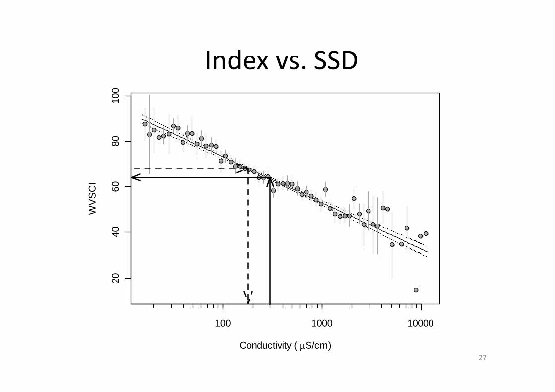
Conductivity ( S/cm)
WV
SC
I
100 1000 10000
20
40
60
80
100
27
Index vs. SSD

Number of binsused to set weights
20 40 60 80 100
200
250
300
350
400
bin size
HC
05
µS/cm
1/3 fewer bins 280
1/3 more bins 30328

Other Analytical Methods
29
Method µS/cm
GAM derived XC95s 270
Quadratic logistic XC95s 275
Titan change point 277
J. Paul change point 292
J. Gerritsen change point 267
C. dubia mortality D. Mount mixture model 1,023
C. dubia LC50 ambient water 2,500

Endpoint:Alternative Levels of Protection
30
HC Level(% species loss)
PointEstimate
(µS/cm)
95% ConfidenceInterval(µS/cm)
HC02 224 137-253
HC05 297 225-305
HC10 335 295-400
HC15 461 375-521

The model was validated with an independentdata set and met the criteria of probablecausation and minimal confounding
EPA-approved methodfor developing WaterQuality (WQ)benchmarks.
31
• Provides methods for• Deriving the HC05
• Assessing Causation• Assessing Potential
Confounding• Model Evaluation