survey over image thresholding techniques and...

Journal of Electronic Imaging 13(1), 146–165 (January 2004).

Survey over image thresholding techniquesand quantitative performance evaluation

Mehmet SezginTubıtak Marmara Research Center

Information Technologies Research InstituteGebze, Kocaeli

TurkeyE-mail: [email protected]

Bulent SankurBogazici University

Electric-Electronic Engineering DepartmentBebek, I˙stanbul

Turkey

elsntk-tives osis

ing

ecel

dd

-

o

m-cts,f ae-theis,

mi-, orbytedinob-thea-g al-k-s.l-weob-ixthea-a-

n,we

ng,de-

ralhetu-

ffectas

3; a

Abstract. We conduct an exhaustive survey of image thresholdingmethods, categorize them, express their formulas under a uniformnotation, and finally carry their performance comparison. Thethresholding methods are categorized according to the informationthey are exploiting, such as histogram shape, measurement spaceclustering, entropy, object attributes, spatial correlation, and localgray-level surface. 40 selected thresholding methods from variouscategories are compared in the context of nondestructive testingapplications as well as for document images. The comparison isbased on the combined performance measures. We identify thethresholding algorithms that perform uniformly better over nonde-structive testing and document image applications. © 2004 SPIE andIS&T. [DOI: 10.1117/1.1631316]

1 Introduction

In many applications of image processing, the gray levof pixels belonging to the object are substantially differefrom the gray levels of the pixels belonging to the bacground. Thresholding then becomes a simple but effectool to separate objects from the background. Examplethresholding applications are document image analywhere the goal is to extract printed characters,1,2 logos,graphical content, or musical scores: map processwhere lines, legends, and characters are to be found:3 sceneprocessing, where a target is to be detected:4 and qualityinspection of materials,5,6 where defective parts must bdelineated. Other applications can be listed as follows:images7,8 and knowledge representation,9 segmentation ofvarious image modalities for nondestructive testing~NDT!applications, such as ultrasonic images in Ref. 10, ecurrent images,11 thermal images,12 x-ray computed tomog-raphy~CAT!,13 endoscopic images,14 laser scanning confo

Paper 02016 received Feb. 7, 2002; revised manuscript received Jan. 23, 200cepted for publication May 27, 2003.1017-9909/2004/$15.00 © 2004 SPIE and IS&T.

146 / Journal of Electronic Imaging / January 2004 / Vol. 13(1)

f,

,

l

y

cal microscopy,13 extraction of edge field,15 image segmen-tation in general,16,17spatio-temporal segmentation of videimages,18 etc.

The output of the thresholding operation is a binary iage whose one state will indicate the foreground objethat is, printed text, a legend, a target, defective part omaterial, etc., while the complementary state will corrspond to the background. Depending on the application,foreground can be represented by gray-level 0, thatblack as for text, and the background by the highest lunance for document paper, that is 255 in 8-bit imagesconversely the foreground by white and the backgroundblack. Various factors, such as nonstationary and correlanoise, ambient illumination, busyness of gray levels withthe object and its background, inadequate contrast, andject size not commensurate with the scene, complicatethresholding operation. Finally, the lack of objective mesures to assess the performance of various thresholdingorithms, and the difficulty of extensive testing in a tasoriented environment, have been other major handicap

In this study we develop taxonomy of thresholding agorithms based on the type of information used, andassess their performance comparatively using a set ofjective segmentation quality metrics. We distinguish scategories, namely, thresholding algorithms based onexploitation of: 1. histogram shape information, 2. mesurement space clustering, 3. histogram entropy informtion, 4. image attribute information, 5. spatial informatioand 6. local characteristics. In this assessment studyenvisage two major application areas of thresholdinamely document binarization and segmentation of nonstructive testing~NDT! images.

A document image analysis system includes seveimage-processing tasks, beginning with digitization of tdocument and ending with character recognition and naral language processing. The thresholding step can aquite critically the performance of successive steps such

c-

the

stioth

ldin.heh aascaningoticeDT

esheceIn

ndm

hos-

eest

ened

thiheiningann-im

cetive, aforite-

u-dof

fors:In

sedseveseThpass

11

ac-at-

ple,ed

velanda

usere-bi-

e ofedci-

is-

ixel

am

e,y-

amofre-e

i-re-

rs. Inhance

-

d

Survey over image thresholding techniques . . .

classification of the document into text objects, andcorrectness of the optical character recognition~OCR!. Im-proper thresholding causes blotches, streaks, erasurethe document confounding segmentation, and recognitasks. The merges, fractures, and other deformations incharacter shapes as a consequence of incorrect threshoare the main reasons of OCR performance deterioratio

In NDT applications, the thresholding is again often tfirst critical step in a series of processing operations sucmorphological filtering, measurement, and statisticalsessment. In contrast to document images, NDT imagesderive from various modalities, with differing applicatiogoals. Furthermore, it is conjectured that the thresholdalgorithms that apply well for document images are nnecessarily the good ones for the NDT images, and vversa, given the different nature of the document and Nimages.

There have been a number of survey papers on throlding. Lee, Chung, and Park19 conducted a comparativanalysis of five global thresholding methods and advanuseful criteria for thresholding performance evaluation.an earlier work, Weszka and Rosenfeld20 also defined sev-eral evaluation criteria. Palumbo, Swaminathan aSrihari21 addressed the issue of document binarization coparing three methods, while Trier and Jain3 had the mostextensive comparison basis~19 methods! in the context ofcharacter segmentation from complex backgrounds. Saet al.22 surveyed nine thresholding algorithms and illutrated comparatively their performance. Glasbey23 pointedout the relationships and performance differences betw11 histogram-based algorithms based on an extensivetistical study.

This survey and evaluation, on the one hand, represa timely effort, in that about 60% of the methods discussand referenced are dating after the last surveys inarea.19,23 We describe 40 thresholding algorithms with tidea underlying them, categorize them according to theformation content used, and describe their thresholdfunctions in a streamlined fashion. We also measurerank their performance comparatively in two different cotexts, namely, document images and NDT images. Theage repertoire consists of printed circuit board~PCB! im-ages, eddy current images, thermal images, microscopeimages, ultrasonic images, textile images, and reflecsurfaces as in ceramics, microscope material imageswell as several document images. For an objective permance comparison, we employ a combination of five crria of shape segmentation goodness.

The outcome of this study is envisaged to be the formlation of the large variety of algorithms under a unifienotation, the identification of the most appropriate typesbinarization algorithms, and deduction of guidelinesnovel algorithms. The structure of the work is as followNotation and general formulations are given in Sec. 2.Secs. 3 to 8, respectively, histogram shape-baclustering-based, entropy-based, object attribute-baspatial information-based, and finally locally adaptithresholding methods are described. In Sec. 9 we prethe comparison methodology and performance criteria.evaluation results of image thresholding methods, serately for nondestructive inspection and document proce

onneng

s-n

-

d

-

o

na-

ts

s

-

d

-

ll

s-

,d,

nte--

ing applications, are given in Sec. 10. Finally, Sec.draws the main conclusions.

2 Categories and Preliminaries

We categorize the thresholding methods in six groupscording to the information they are exploiting. These cegories are:

1. histogram shape-based methods, where, for examthe peaks, valleys and curvatures of the smoothhistogram are analyzed

2. clustering-based methods, where the gray-lesamples are clustered in two parts as backgroundforeground~object!, or alternately are modeled asmixture of two Gaussians

3. entropy-based methods result in algorithms thatthe entropy of the foreground and backgroundgions, the cross-entropy between the original andnarized image, etc.

4. object attribute-based methods search a measursimilarity between the gray-level and the binarizimages, such as fuzzy shape similarity, edge coindence, etc.

5. the spatial methods use higher-order probability dtribution and/or correlation between pixels

6. local methods adapt the threshold value on each pto the local image characteristics.

In the sequel, we use the following notation. The histogrand the probability mass function~PMF! of the image areindicated, respectively, byh(g) and by p(g), g50...G,where G is the maximum luminance value in the imagtypically 255 if 8-bit quantization is assumed. If the gravalue range is not explicitly indicated as@gmin , gmax], itwill be assumed to extend from 0 toG. The cumulativeprobability function is defined as

P~g!5(i 50

g

p~ i !.

It is assumed that the PMF is estimated from the histogrof the image by normalizing it to the total numbersamples. In the context of document processing, the foground ~object! becomes the set of pixels with luminancvalues less thanT, while the background pixels have lumnance value above this threshold. In NDT images, the foground area may consists of darker~more absorbent,denser, etc.! regions or conversely of shinier regions, foexample, hotter, more reflective, less dense, etc., regionthe latter contexts, where the object appears brighter tthe background, obviously the set of pixels with luminangreater thanT will be defined as the foreground.

The foreground~object! and background PMFs are expressed aspf(g), 0<g<T, andpb(g), T11<g<G, re-spectively, whereT is the threshold value. The foregrounand background area probabilities are calculated as:

Pf~T!5Pf5 (g50

T

p~g!, Pb~T!5Pb5 (g5T11

G

p~g!. ~1!

Journal of Electronic Imaging / January 2004 / Vol. 13(1) / 147

Sezgin and Sankur

148 / Journal of Ele

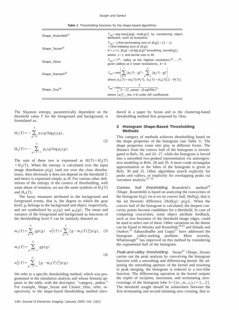
Table 1 Thresholding functions for the shape-based algorithms.

Shape–Rosenfeld24 Topt5arg max$@p(g)2Hull(g)#% by considering objectattributes, such as busyness.

Shape–Sezan32

Topt5g$first terminating zero of p(g)%1(12g)3$first initiating zero of p(g)%0<g<1, p(g)5d/dg@p(g)* smoothing–kernel(g)#,where g51 and kernel size is 55

Shape–Olivio Topt5^T0, valley at the highest resolutionuT1,...Tk,given valleys at k lower resolutions&, k53

Shape–Ramesh30 Topt5minF(g50

T

@b1~T!2g#21 (g5T11

G

@b2~T!2g#2Gwhere b1(T)5mf(T)/P(T), b2(T)5mb(T)@12P(T)#

Shape–Guo28 Topt5ming

1

u12(i51p aiexp~2j2pg/256!u2 ,

where $ai% i51p the n’th order AR coefficients

this

ut-

th

andrayely

s o

ro-ap

tro

sed

on

heti-edres-larin

foria

of

on-e ofck,ouldeme

ely,g

amd-ingbets

o-

theis:

The Shannon entropy, parametrically dependent onthreshold valueT for the foreground and background,formulated as:

H f~T!52 (g50

T

pf~g!log pf~g!,

~2!

Hb~T!52 (g5T11

G

pb~g!log pb~g!.

The sum of these two is expressed asH(T)5H f(T)1Hb(T). When the entropy is calculated over the inpimage distributionp(g) ~and not over the class distributions!, then obviously it does not depend on the thresholdT,and hence is expressed simply asH. For various other defi-nitions of the entropy in the context of thresholding, wisome abuse of notation, we use the same symbols ofH f(T)andHb(T).

The fuzzy measures attributed to the backgroundforeground events, that is, the degree to which the glevel,g, belongs to the background and object, respectivand are symbolized bym f(g) and mb(g). The mean andvariance of the foreground and background as functionthe thresholding levelT can be similarly denoted as:

mf~T!5 (g50

T

gp~g! s f2~T!5 (

g50

T

@g2mf~T!#2p~g!, ~3!

mb~T!5 (g5T11

G

gp~g!

~4!

sb2~T!5 (

g5T11

G

@g2mb~T!#2p~g!.

We refer to a specific thresholding method, which was pgrammed in the simulation analysis and whose formulapears in the table, with the descriptor, ‘‘category–author.’’For example, Shape–Sezan and Cluster–Otsu, refer, re-spectively, to the shape-based thresholding method in

ctronic Imaging / January 2004 / Vol. 13(1)

e

,

f

-

-

duced in a paper by Sezan and to the clustering-bathresholding method first proposed by Otsu.

3 Histogram Shape-Based ThresholdingMethods

This category of methods achieves thresholding basedthe shape properties of the histogram~see Table 1!. Theshape properties come into play in different forms. Tdistance from the convex hull of the histogram is invesgated in Refs. 20, and 24–27, while the histogram is forcinto a smoothed two-peaked representation via autoregsive modeling in Refs. 28 and 29. A more crude rectanguapproximation to the lobes of the histogram is givenRefs. 30 and 31. Other algorithms search explicitlypeaks and valleys, or implicitly for overlapping peaks vcurvature analysis.32–34

Convex hull thresholding. Rosenfeld’s method24

~Shape–Rosenfeld! is based on analyzing the concavitiesthe histogramh(g) vis-a-vis its convex hull, Hull~g!, that isthe set theoretic differenceuHull(g)2p(g)u. When theconvex hull of the histogram is calculated, the deepest ccavity points become candidates for a threshold. In cascompeting concavities, some object attribute feedbasuch as low busyness of the threshold image edges, cbe used to select one of them. Other variations on the thcan be found in Weszka and Rosenfeld,20,25and Halada andOsokov.26 Sahasrabudhe and Gupta27 have addressed thhistogram valley-seeking problem. More recentWhatmough35 has improved on this method by considerinthe exponential hull of the histogram.

Peak-and-valley thresholding. Sezan32 ~Shape–Sezan!carries out the peak analysis by convolving the histogrfunction with a smoothing and differencing kernel. By ajusting the smoothing aperture of the kernel and resortto peak merging, the histogram is reduced to a two-lofunction. The differencing operation in the kernel outputhe triplet of incipient, maximum, and terminating zercrossings of the histogram lobeS5@(ei ,mi ,si),i 51,...2#.The threshold sought should be somewhere betweenfirst terminating and second initiating zero crossing, that

isandised-sttureto

retandadisis

e

oldromintoto

i-ushis

epo-. A

rene

ony,

rsed

iniult-

ssetwo

s-ile47.

lass

andate

the

tinof

ri-lish-of

sultsach

fer-ld-

nd.

tured

ityrord

-um-o,isari-

aen-

ingter


Topt5ge11(12g)s2 , 0<g<1. In our work, we havefound that g51 yields good results. Variations on ththeme are provided in Boukharouba, Rebordao,Wendel,36 where the cumulative distribution of the imagefirst expanded in terms of Tschebyshev functions, followby the curvature analysis. Tsai37 obtains a smoothed histogram via Gaussians, and the resulting histogram is invegated for the presence of both valleys and sharp curvapoints. We point out that the curvature analysis becomeffective when the histogram has lost its bimodality duethe excessive overlapping of class histograms.

In a similar vein, Carlotto33 and Olivo34 ~Shape–Olivio!considerthe multiscale analysis of the PMF and interpits fingerprints, that is, the course of its zero crossingsextrema over the scales. In Ref. 34 using a discrete dywavelet transform, one obtains the multiresolution analyof the histogram,ps(g)5p(g)* cs(g), s51,2..., wherep0(g)5p(g) is the original normalized histogram. Ththreshold is defined as the valley~minimum! point follow-ing the first peak in the smoothed histogram. This threshposition is successively refined over the scales starting fthe coarsest resolution. Thus starting with the valley poT(k) at thek’th coarse level, the position is backtrackedthe corresponding extrema in the higher resolution hisgramsp(k21)(g)...p(0)(g), that is,T(0) is estimated by re-fining the sequenceT(1)...T(k) ~in our work k53 wasused!.

Shape-modeling thresholding. Ramesh, Yoo, andSethi30 ~Shape–Ramesh! use a simple functional approxmation to the PMF consisting of a two-step function. Ththe sum of squares between a bilevel function and thetogram is minimized, and the solution forTopt is obtainedby iterative search. Kampke and Kober31 have generalizedthe shape approximation idea.

In Cai and Liu,29 the authors have approximated thspectrum as the power spectrum of multi-complex exnential signals using Prony’s spectral analysis methodsimilar all-pole model was assumed in Guo28 ~Shape–Guo!.We have used a modified approach, where an autoregsive ~AR! model is used to smooth the histogram. Here obegins by interpreting the PMF and its mirror reflectiaroundg50, p(2g), as a noisy power spectral densitgiven by p(g)5p(g) for g>0, andp(2g) for g<0. Onethen obtains the autocorrelation coefficients at lagsk50...G, by the inverse discrete fourier transform~IDFT! ofthe original histogram, that is,r (k)5IDFT@ p(g)#. The au-tocorrelation coefficients$r (k)% are then used to solve fothen’th order AR coefficients$ai%. In effect, one smoothethe histogram and forces it to a bimodal or two-peakrepresentation via then’th order AR model (n51,2,3,4,5,6). The threshold is established as the mmum, resting between its two pole locations, of the resing smoothed AR spectrum.

4 Clustering-Based Thresholding Methods

In this class of algorithms, the gray-level data undergoeclustering analysis, with the number of clusters beingalways to two. Since the two clusters correspond to the

i-es

c

t

-

-

s-

-

at

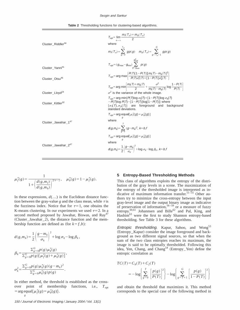
lobes of a histogram~assumed distinct!, some authorssearch for the midpoint of the peaks.38–41 In Refs. 42–45,the algorithm is based on the fitting of the mixture of Gausians. Mean-square clustering is used in Ref. 46, whfuzzy clustering ideas have been applied in Refs. 30 andSee Table 2 for these algorithms.

Iterative thresholding. Riddler38 ~Cluster–Riddler! ad-vanced one of the first iterative schemes based on two-cGaussian mixture models. At iterationn, a new thresholdTn is established using the average of the foregroundbackground class means. In practice, iterations terminwhen the changesuTn2Tn11u become sufficiently small.Leung and Fam39 and Trussel40 realized two similar meth-ods. In his method, Yanni and Horne41 ~Cluster–Yanni! ini-tializes the midpoint between the two assumed peaks ofhistogram asgmid5(gmax1gmin)/2, wheregmax is the high-est nonzero gray level andgmin is the lowest one, so tha(gmax2gmin) becomes the span of nonzero gray valuesthe histogram. This midpoint is updated using the meanthe two peaks on the right and left, that is, asgmid*5(gpeak11gpeak2)/2.

Clustering thresholding. Otsu46 ~Cluster–Otsu! sug-gested minimizing the weighted sum of within-class vaances of the foreground and background pixels to estaban optimum threshold. Recall that minimization of withinclass variances is tantamount to the maximizationbetween-class scatter. This method gives satisfactory rewhen the numbers of pixels in each class are close to eother. The Otsu method still remains one of the most reenced thresholding methods. In a similar study, threshoing based on isodata clustering is given in Velasco.48 Somelimitations of the Otsu method are discussed in Lee aPark.49 Liu and Li50 generalized it to a 2-D Otsu algorithm

Minimum error thresholding. These methodsassume that the image can be characterized by a mixdistribution of foreground and backgrounpixels: p(g)5P(T).pf(g)1@12P(T)#.pb(g). Lloyd42

~Cluster–Lloyd! considers equal variance Gaussian densfunctions, and minimizes the total misclassification ervia an iterative search. In contrast, Kittler anIllingworth43,45 ~Cluster–Kittler! removes the equal variance assumption and, in essence, addresses a minimerror Gaussian density-fitting problem. Recently ChHaralick, and Yi44 have suggested an improvement of ththresholding method by observing that the means and vances estimated from truncated distributions result inbias. This bias becomes noticeable, however, only whever the two histogram modes are not distinguishable.

Fuzzy clustering thresholding. Jawahar, Biswas, andRay47 ~Cluster–Jawahar–1!, and Ramesh Yoo, and Sethi30

assign fuzzy clustering memberships to pixels dependon their differences from the two class means. The clusmeans and membership functions are calculated as:

mk5(g50

G g.p~g!mkt~g!

(g50G p~g!mk

t~g!, k5 f ,b,


g

Sezgin and Sankur


Table 2 Thresholding functions for clustering-based algorithms.

Cluster–Riddler34

Topt5 limn→`

mf~Tn!1mb~Tn!

2

where

mf~Tn!5(g50

Tn

gp~g ! mb~Tn!5 (g5Tn11

G

gp~g !

Cluster–Yanni41Topt5~gmax2gmin! (

g5gmin

gmid*

p~g !

Cluster–Otsu46Topt5arg maxHP~T!@12P~T!#@mf~T!2mb~T!#2

P~T!sf2~T!1@12P~T!#sb

2~T! J

Cluster–Lloyd24

Topt5arg minFmf~T!1mb~T!

21

s2

mf~T!2mb~T!log

12P~T!

P~T! Gs2 is the variance of the whole image.

Cluster–Kittler32

Topt5arg min$P(T)log sf(T)1@12P(T)#log sb(T)2P(T)log P(T)2@12P(T)#log@12P(T)#% where$s f(T),sb(T)% are foreground and backgroundstandard deviations.

Cluster–Jawahar–147

Topt5arg equalg

@m ft(g)5mb

t (g)#

where

d~g,mk!5(g50

T

~g2mk!2, k5b,f

Cluster–Jawahar–247

Topt5arg equalg

@m ft(g)5mb

t (g)#

where

d~g,mk!51

2 Sg2mk

skD2

1log sk2log bk , k5b,f

-

ay-

os

ri-ofin-

putive

ed

k-thetheis

odin

m ft~g!5

1

11S d~g,mf !

d~g,mb! D2/t21 , mb

t~g!512m ft~g!.

In these expressions,d(...) is theEuclidean distance function between the gray-valueg and the class mean, whilet isthe fuzziness index. Notice that fort51, one obtains theK-means clustering. In our experiments we usedt52. In asecond method proposed by Jawahar, Biswas, and R47

~Cluster–Jawahar–2!, the distance function and the membership function are defined as~for k5 f ,b):

d~g,mk!51

2 S g2mk

skD 2

1 logsk2 logbk ,

bk5(g50

G p~g!mkt~g!

(g50G p~g!@m f

t~g!1mbt~g!#

,

sk25

(g50G p~g!mk

t~g!~g2mk!2

(g50G mk

t~g!p~g!.

In either method, the threshold is established as the crover point of membership functions, i.e.,Topt

5arg equal$m ft(g)5mb

t(g)%.


s-

5 Entropy-Based Thresholding Methods

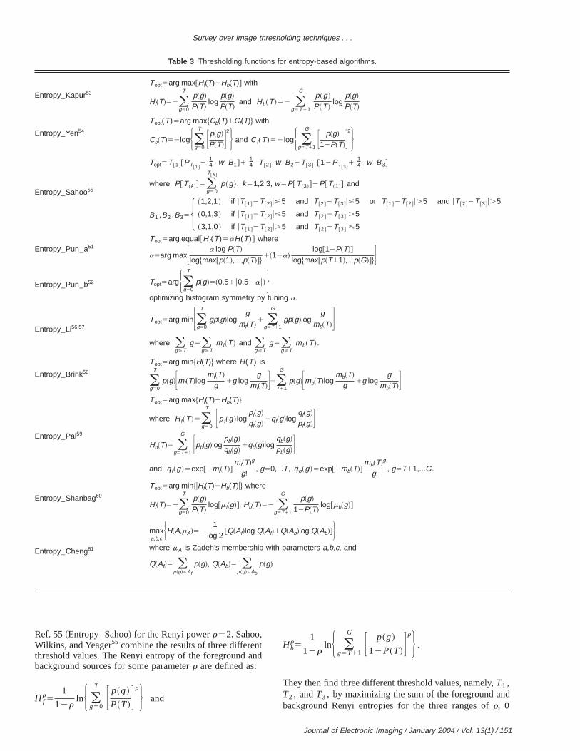
This class of algorithms exploits the entropy of the distbution of the gray levels in a scene. The maximizationthe entropy of the thresholded image is interpreted asdicative of maximum information transfer.51–55 Other au-thors try to minimize the cross-entropy between the ingray-level image and the output binary image as indicatof preservation of information,56–59 or a measure of fuzzyentropy.60,61 Johannsen and Bille62 and Pal, King, andHashim63 were the first to study Shannon entropy-basthresholding. See Table 3 for these algorithms.

Entropic thresholding. Kapur, Sahoo, and Wong53

~Entropy–Kapur! consider the image foreground and bacground as two different signal sources, so that whensum of the two class entropies reaches its maximum,image is said to be optimally thresholded. Following thidea, Yen, Chang, and Chang54 ~Entropy–Yen! define theentropic correlation as

TC~T!5Cb~T!1Cf~T!

52 logH (g50

T F p~g!

P~T!G2J 2 logH (

g5T11

G F p~g!

12P~T!G2J

and obtain the threshold that maximizes it. This methcorresponds to the special case of the following method


Table 3 Thresholding functions for entropy-based algorithms.

Entropy–Kapur53

Topt5arg max@Hf(T)1Hb(T)# with

Hf~T!52(g50

Tp~g!

P~T!log

p~g!

P~T!and Hb~T !52 (

g5T11

Gp~g !

P~T !log

p~g!

P~T!

Entropy–Yen54

Topt(T)5arg max$Cb(T)1Cf(T)% with

Cb~T!52logH(g50

T Fp~g!

P~T!G2J and Cf~T !52 logH (

g5T11

G F p~g!

12P~T!G2J

Entropy–Sahoo55

Topt5T @1#@PT@1#1

14 •w•B1#1

14 •T @2#•w•B21T @3#•@12PT@3#

114 •w•B3#

where P@T ~k !#5(g50

T@k#

p~g !, k51,2,3, w5P@T ~3 !#2P@T ~1 !# and

B1 ,B2 ,B35H ~1,2,1 ! if uT @1#2T @2#u<5 and uT @2#2T @3#u<5 or uT @1#2T @2#u.5 and uT @2#2T @3#u.5

~0,1,3 ! if uT @1#2T @2#u<5 and uT @2#2T @3#u.5

~3,1,0 ! if uT @1#2T @2#u.5 and uT @2#2T @3#u<5

Entropy–Pun–a51Topt5arg equal@Hf(T)5aH(T)# where

a5arg maxF a log P~T!

log$max@p~1!,...,p~T!#%1~12a!

log@12P~T!#

log$max@p~T11!,...p~G!#%GEntropy–Pun–b52 Topt5argH(

g50

T

p~g!5~0.51u0.52au!Joptimizing histogram symmetry by tuning a.

Entropy–Li56,57Topt5arg minF(

g50

T

gp~g!logg

mf~T!1 (

g5T11

G

gp~g!logg

mb~T!Gwhere (

g<Tg5(

g<Tmf~T ! and (

g>Tg5(

g>Tmb~T !.

Entropy–Brink58

Topt5arg min$H(T)% where H(T) is

(g50

T

p~g!Fmf~T!logmf~T!

g1g log

gmf~T!G1(

T11

G

p~g!Fmb~T!logmb~T!

g1g log

gmb~T!G

Entropy–Pal59

Topt5arg max$Hf(T)1Hb(T)%

where Hf~T !5(g50

T Fpf~g !logpf~g!

qf~g!1qf~g!log

qf~g!

pf~g!GHb~T!5 (

g5T11

G Fpb~g!logpb~g!

qb~g!1qb~g!log

qb~g!

pb~g!Gand qf~g !5exp@2mf~T!#

mf~T!g

g!, g50,...T, qb~g !5exp@2mb~T!#

mb~T!g

g!, g5T11,...G.

Entropy–Shanbag60

Topt5arg min$uHf(T)2Hb(T)u% where

Hf~T!52(g50

Tp~g!

P~T!log@mf~g!#, Hb~T!52 (

g5T11

Gp~g!

12P~T!log@mb~g!#

Entropy–Cheng61

maxa,b,c

HH~A,mA!521

log 2@Q~Af!log Q~Af!1Q~Ab!log Q~Ab!#J

where mA is Zadeh’s membership with parameters a,b,c, and

Q~Af!5 (m~g!PAf

p~g!, Q~Ab!5 (m~g!PAb

p~g!

tnd

d

Ref. 55~Entropy–Sahoo! for the Renyi powerr52. Sahoo,Wilkins, and Yeager55 combine the results of three differenthreshold values. The Renyi entropy of the foreground abackground sources for some parameterr are defined as:

H fr5

1

12rlnH (

g50

T F p~g!

P~T!GrJ and

Hbr5

1

12rlnH (

g5T11

G F p~g!

12P~T!GrJ .

They then find three different threshold values, namely,T1 ,T2 , andT3 , by maximizing the sum of the foreground anbackground Renyi entropies for the three ranges ofr, 0


at

, w

ally

t--

a-is

onei

ne

coesnd. Aifi-

ns:

of

anhey a

and

by

tonty,

-

re-odt

Za--

-

Sezgin and Sankur

,r,1, r.1, andr51, respectively. For exampleT2 forr51 corresponds to the Kapur, Sahoo and Wong53 thresh-old value, while forr.1, the threshold corresponds to thfound in Yen, Chang, and Chang.54 DenotingT@1# , T@2# ,andT@3# as the rank orderedT1 , T2 , andT3 values, ‘‘op-timum’’ T is found by their weighted combination.

Finally, although the two methods of Pun51,52 have beensuperseded by other techniques, for historical reasonshave included them~Entropy–Pun1, Entropy–Pun2!. InRef. 51, Pun considers the gray-level histogram asG-symbol source, where all the symbols are statisticaindependent. He considers the ratio of thea posteriorien-tropy H8(T)52P(T)log@P(T)#2@12P(T)#log@12P(T)# asa function of the thresholdT to that of the source entropy

H~T!52 (g50

T

p~g!log@p~g!#2 (g5T11

G

p~g!log@p~g!#.

This ratio is lower bounded by

H8~T!

H>F a log P~T!

log$max@p~1!,...,p~T!#%

1~12a!log~12P~T!!

log$max@p~T11!,...p~G!#%G .In a second method, the threshold52 depends on the anisoropy parametera, which depends on the histogram asymmetry.

Cross-entropic thresholding. Li, Lee, and Tam56,57

~Entropy–Li ! formulate the thresholding as the minimiztion of an information theoretic distance. This measurethe Kullback-Leibler distance

D~q,p!5( q~g!logq~g!

p~g!

of the distributions of the observed imagep(g) and of thereconstructed imageq(g). The Kullback-Leibler measureis minimized under the constraint that observed and recstructed images have identical average intensity in thforeground and background, namely the condition

(g<T

g5 (g<T

mf~T! and (g>T

g5 (g>T

mb~T!.

Brink and Pendock58 ~Entropy–Brink! suggest that athreshold be selected to minimize the cross-entropy, defias

H~T!5 (g50

T

q~g!logq~g!

p~g!1 (

g5T11

G

p~g!logp~g!

q~g!.

The cross-entropy is interpreted as a measure of datasistency between the original and the binarized imagThey show that this optimum threshold can also be fouby maximizing an expression in terms of class meansvariation of this cross-entropy approach is given by speccally modeling thea posterioriPMF of the foreground and


e

-r

d

n-.

background regions, as in Pal59 ~Entropy–Pal!. Using themaximum entropy principle in Shore and Johanson,64 thecorresponding PMFs are defined in terms of class mea

qf~g!5exp@2mf~T!#mf~T!g

g!, g50,...T,

qb~g!5exp@2mb~T!#mb~T!g

g!, g5T11,...G.

Wong and Sahoo65 have also presented a former studythresholding based on the maximum entropy principle.

Fuzzy entropic thresholding. Shanbag60

~Entropy–Shanbag! considers the fuzzy memberships asindication of how strongly a gray value belongs to tbackground or to the foreground. In fact, the farther awagray value is from a presumed threshold~the deeper in itsregion!, the greater becomes its potential to belong tospecific class. Thus, for any foreground and backgroupixel, which is i levels below ori levels above a giventhresholdT, the membership values are determined by

m f~T2 i !50.51p~T!1...1p~T212 i !1p~T2 i !

2P~T!,

that is, its measure of belonging to the foreground, and

mb~T1 i !50.51p~T11!1...1p~T211 i !1p~T1 i !

2~12P~T!!,

respectively. Obviously on the gray value correspondingthe threshold, one should have the maximum uncertaisuch thatm f(T)5mb(T)50.5. The optimum threshold isfound as theT that minimizes the sum of the fuzzy entropies,

Topt5arg minT

$uH0~T!2H1~T!u%,

H0~T!52 (g50

Tp~g!

P~T!log@m0~g!#,

H1~T!52 (g5T11

Gp~g!

12P~T!log@m1~g!#,

since one wants to get equal information for both the foground and background. Cheng, Chen, and Sun’s meth61

~Entropy–Cheng! relies on the maximization of fuzzy evenentropies, namely, the foregroundAf and backgroundAbsubevents. The membership function is assigned usingdeh’s S function in Ref. 66. The probability of the foreground subeventQ(Af) is found by summing those grayvalue probabilities that map into theAf subevent:

Q~Af !5 (m~g!PAf

p~g!


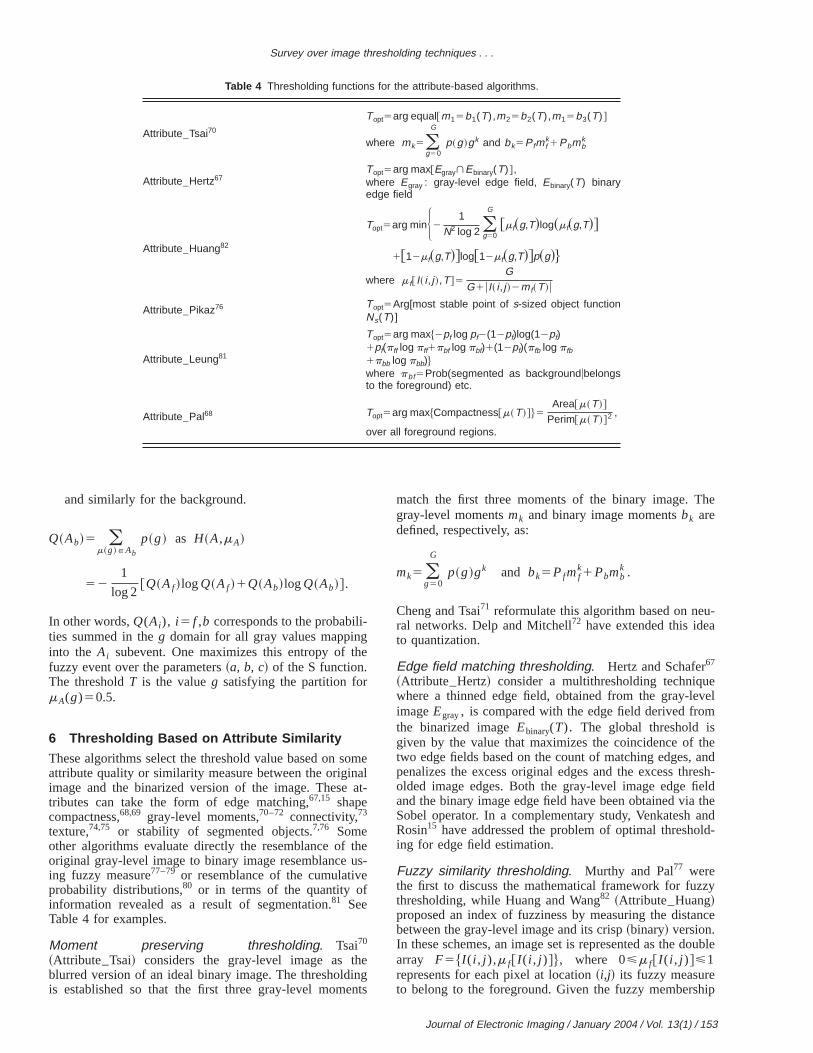
Table 4 Thresholding functions for the attribute-based algorithms.

Attribute–Tsai70

Topt5arg equal@m15b1(T),m25b2(T),m15b3(T)#

where mk5(g50

G

p~g !gk and bk5Pfmfk1Pbmb

k

Attribute–Hertz67Topt5arg max@EgrayùEbinary(T)#,where Egray : gray-level edge field, Ebinary(T) binaryedge field

Attribute–Huang82

Topt5arg minH21

N2 log 2 (g50

G

@mf~g,T!log~mf~g,T!#

1@12mf~g,T!#log@12mf~g,T!#p~g!%

where m f@ I~ i , j !,T#5G

G1uI~ i , j !2mf~T !u

Attribute–Pikaz76 Topt5Arg[most stable point of s-sized object functionNs(T)]

Attribute–Leung81

Topt5arg max$2pf log pf2(12pf)log(12pf)1pf(pff log pff1pbf log pbf)1(12pf)(pfb log pfb

1pbb log pbb)%where pbf5Prob(segmented as backgroundubelongsto the foreground) etc.

Attribute–Pal68 Topt5arg max$Compactness@m~T !#%5Area@m~T !#

Perim@m~T !#2 ,

over all foreground regions.

i-ghe

omalat

theuse

heingnt

he

u-a

evelm

theandresh-eldthe

andld-

zy

nce

ouble

hip

and similarly for the background.

Q~Ab!5 (m~g!PAb

p~g! as H~A,mA!

521

log 2@Q~Af !logQ~Af !1Q~Ab!logQ~Ab!#.

In other words,Q(Ai), i 5 f ,b corresponds to the probabilties summed in theg domain for all gray values mappininto the Ai subevent. One maximizes this entropy of tfuzzy event over the parameters~a, b, c! of the S function.The thresholdT is the valueg satisfying the partition formA(g)50.5.

6 Thresholding Based on Attribute Similarity

These algorithms select the threshold value based on sattribute quality or similarity measure between the originimage and the binarized version of the image. Thesetributes can take the form of edge matching,67,15 shapecompactness,68,69 gray-level moments,70–72 connectivity,73

texture,74,75 or stability of segmented objects.7,76 Someother algorithms evaluate directly the resemblance oforiginal gray-level image to binary image resemblanceing fuzzy measure77–79 or resemblance of the cumulativprobability distributions,80 or in terms of the quantity ofinformation revealed as a result of segmentation.81 SeeTable 4 for examples.

Moment preserving thresholding. Tsai70

~Attribute–Tsai! considers the gray-level image as tblurred version of an ideal binary image. The thresholdis established so that the first three gray-level mome

e

-

-

s

match the first three moments of the binary image. Tgray-level momentsmk and binary image momentsbk aredefined, respectively, as:

mk5 (g50

G

p~g!gk and bk5Pfmfk1Pbmb

k .

Cheng and Tsai71 reformulate this algorithm based on neral networks. Delp and Mitchell72 have extended this ideto quantization.

Edge field matching thresholding. Hertz and Schafer67

~Attribute–Hertz! consider a multithresholding techniquwhere a thinned edge field, obtained from the gray-leimageEgray, is compared with the edge field derived frothe binarized imageEbinary(T). The global threshold isgiven by the value that maximizes the coincidence oftwo edge fields based on the count of matching edges,penalizes the excess original edges and the excess tholded image edges. Both the gray-level image edge fiand the binary image edge field have been obtained viaSobel operator. In a complementary study, VenkateshRosin15 have addressed the problem of optimal threshoing for edge field estimation.

Fuzzy similarity thresholding. Murthy and Pal77 werethe first to discuss the mathematical framework for fuzthresholding, while Huang and Wang82 ~Attribute–Huang!proposed an index of fuzziness by measuring the distabetween the gray-level image and its crisp~binary! version.In these schemes, an image set is represented as the darray F5$I ( i , j ),m f@ I ( i , j )#%, where 0<m f@ I ( i , j )#<1represents for each pixel at location~i,j! its fuzzy measureto belong to the foreground. Given the fuzzy members


leag

i-ss

foruandin

shth

esize

g athe

hengmes

etiontio

theis

matioer

eg-atiob-

the

n-xiega

zyed

ero-

eter

thetheat

agenesstial

s.ri,a-

or-

tenngcbi-

ngre-allongic.in

ar-ovs is

ri-forn

en-t to,ng.hethe

en-elsiathe

cal

Sezgin and Sankur

value for each pixel, an index of fuzziness for the whoimage can be obtained via the Shannon entropy or the Yer’s measure.78 The optimum threshold is found by minmizing the index of fuzziness defined in terms of cla~foreground, background! medians or meansmf(T), mb(T)and membership functionsm f@ I ( i , j ),T#, mb@ I ( i , j ),T#. Ra-mar et al.79 have evaluated various fuzzy measuresthreshold selection, namely linear index of fuzziness, qdratic index of fuzziness, logarithmic entropy measure, aexponential entropy measure, concluding that the lineardex works best.

Topological stable-state thresholding. Russ7 has notedthat experts in microscopy subjectively adjust the threolding level at a point where the edges and shape ofobject get stabilized. Similarly Pikaz and Averbuch76

~Attribute–Pikaz! pursue a threshold value, which becomstable when the foreground objects reach their correct sThis is instrumented via the size-threshold functionNs(T),which is defined as the number of objects possessinleasts number of pixels. The threshold is established inwidest possible plateau of the graph of theNs(T) function.Since noise objects rapidly disappear with shifting tthreshold, the plateau in effect reveals the threshold rafor which foreground objects are easily distinguished frothe background. We chose the middle value of the largsized plateau as the optimum threshold value.

Maximum information thresholding. Leung and Lam81

~Attribute–Leung! define the thresholding problem as thchange in the uncertainty of an observation on specificaof the foreground and background classes. The presentaof any foreground/background information reducesclass uncertainty of a pixel, and this information gainmeasured byH(p)2aH(pf)2(12a)H(pb), whereH(p)is the initial uncertainty of a pixel anda is the probabilityof a pixel to belong to the foreground class. The optimuthreshold is established as that generating a segmentmap that, in turn, minimizes the average residual unctainty about which class a pixel belongs after the smented image has been observed. Such segmentwould obviously minimize the wrong classification proability of pixels, in other words, the false alarmsp f b ~pixelappears in the foreground while actually belonging tobackground! and the miss probabilitypb f . According tothis notationp f f , pbb denote the correct classification coditionals. The optimum threshold corresponds to the mamum decrease in uncertainty, which implies that the smented image carries as close a quantity of informationthat in the original information.

Enhancement of fuzzy compactness thres-holding. Rosenfeld generalized the concept of fuzgeometry.69 For example, the area of a fuzzy set is definas

Area~m!5 (i , j 51

N

m@ I ~ i , j !#

while its perimeter is given by


-

-

-

-e

.

t

e

t

n

n-

n

--s

Perim~m!5 (i , j 51

N

um@ I ~ i , j !#2m@ I ~ i , j 11!#u

1 (i , j 51

N

um@ I ~ i , j !#2m@ I ~ i 11,j !#u,

where the summation is taken over any region of nonzmembership, andN is the number of regions in a segmented image. Pal and Rosenfeld68 ~Attribute–Pal! evalu-ated the segmentation output, such that both the perimand area are functions of the thresholdT. The optimumthreshold is determined to maximize the compactness ofsegmented foreground sets. In practice, one can usestandard S function to assign the membership functionthe pixel I ( i , j ): m@ I ( i , j )#5S@ I ( i , j );a,b,c#, as inKaufmann,66 with crossover pointb5(a1c)/2 and band-width Db5b2a5c2b. The optimum thresholdT isfound by exhaustively searching over the (b,Db) pairs tominimize the compactness figure. Obviously the advantof the compactness measure over other indexes of fuzziis that the geometry of the objects or fuzziness in the spadomain is taken into consideration.

Other studies involving image attributes are as followIn the context of document image binarization, Liu, Srihaand Fenrich74,75have considered document image binariztion based on texture analysis, while Don83 has taken intoconsideration noise attribute of images. Guo84 develops ascheme based on morphological filtering and the fourthder central moment. Solihin and Leedham85 have devel-oped a global thresholding method to extract handwritparts from low-quality documents. In another interestiapproach, Aviad and Lozinskii86 have introduced semantithresholding to emulate the human approach to imagenarization. The semantic threshold is found by minimizimeasures of conflict criteria, so that the binary imagesembles most to a verbal description of the scene. Gand Spinello87 have developed a technique for thresholdiand isocontour extraction using fuzzy arithmetFernandez80 has investigated the selection of a thresholdmatched filtering applications in the detection of small tget objects. In this application, the Kolmogorov-Smirndistance between the background and object histogrammaximized as a function of the threshold value.

7 Spatial Thresholding Methods

This class of algorithms utilizes not only gray value distbution but also dependency of pixels in a neighborhood,example, in the form of context probabilities, correlatiofunctions, cooccurrence probabilities, local linear depdence models of pixels, 2-D entropy, etc. One of the firsexplore spatial information was Kirby and Rosenfeld88

who considered local average gray levels for thresholdiOthers have followed using relaxation to improve on tbinary map as in Refs. 89 and 90, the Laplacian ofimages to enhance histograms,25 the quadtreethresholding,91 and second-order statistics.92 Cooccurrenceprobabilities have been used as indicators of spatial depdence as in Refs. 93–96. The characteristics of ‘‘pixjointly with their local average’’ have been considered vtheir second-order entropy as in Refs. 97–100 and viafuzzy partitioning as in Refs. 101, 102, and 103. The lo


Table 5 Thresholding functions for spatial thresholding methods.

Spatial–Pal–1 andSpatial–Pal–294

Topt5arg max@Hbb(T)1Hff(T)# or Topt5arg max@Hfb(T)1Hbf(T)#where Hfb(T), Hbf(T), Hff(T), Hbb(T) are the co-occurrence entropies

Spatial–Abutaleb97

(Topt ,Topt)5arg min$log@P(T,T)@12P(T,T)#1Hf /P(T,T)

1Hb /@12P(T,T)#%where

Hf52(i51

T

(j51

Tp~g,g!

P~T,T!log

p~g,g!

P~T,T!and

Hb52 (i5T11

G

(j5T11

Gp~g,g!

@12P~T,T!#log

p~g,g!

@12P~T,T!#

Spatial–Beghdadi104

Topt5arg minF2(k50

s3s

pkblock~T !• log pk

block~T !Gwhere pk

block(T) is the probability of s3s size blockscontaining k whites and s22k blacks(s52,4,8,16)

Spatial–Cheng101

Topt5maxa,b,c$Hfuzzy(foreground)1Hfuzzy(background)%

where Hfuzzy~A !52(x,y

mA~x,y !p~x,y !log p~x,y!,

$a,b,c%, the S-function parameters; $A5foreground,background%; $x,y%5$ pixel value, local average valuewithin 333 region%.

b

ef.exSe

foa-

vere,ueus

he

theina-to

as,

he

-thei-

ncelly,

asthe

ec-

-

si-

spatial dependence of pixels is captured in Ref. 104 asnary block patterns. Thresholding based on explicita pos-teriori spatial probability estimation was analyzed in R105, and thresholding as the max-min distance to thetracted foreground object was considered in Ref. 106.Table 5 for these methods.

Cooccurrence thresholding methods. Chanda andMajumder96 have suggested the use of cooccurrencesthreshold selection, and Lie93 has proposed several mesures to this effect. In this vein, Pal94 ~Spatial–Pal!, realiz-ing that two images with identical histograms can yet hadifferent n’th order entropies due to their spatial structuconsidered the cooccurrence probability of the gray valg1 andg2 over its horizontal and vertical neighbors. Ththe pixels, first binarized with threshold valueT, aregrouped into background and foreground regions. Tcooccurrence of gray levelsk andm is calculated as

ck,m5 (all pixels

d, where d51 if

$@ I ~ i , j !5k#∧@ I ~ i , j 11!5m#∨@ I ~ i , j !5k#

∧@ I ~ i 11,j !5m#%,

and d50 otherwise. Pal proposes two methods to usecooccurrence probabilities. In the first expression, the brized image is forced to have as many backgroundforeground and foreground-to-background transitionspossible. In the second approach, the converse is truethat the probability of the neighboring pixels staying in tsame class is rewarded.

i-

-e

r

s

--

in

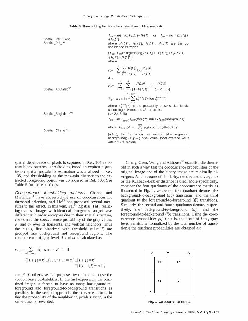
Chang, Chen, Wang and Althouse95 establish the threshold in such a way that the cooccurrence probabilities oforiginal image and of the binary image are minimally dvergent. As a measure of similarity, the directed divergeor the Kullback-Leibler distance is used. More specificaconsider the four quadrants of the cooccurrence matrixillustrated in Fig. 1, where the first quadrant denotesbackground-to-background~bb! transitions, and the thirdquadrant to the foreground-to-foreground~ff ! transitions.Similarly, the second and fourth quadrants denote, resptively, the background-to-foreground~bf ! and theforeground-to-background~fb! transitions. Using the cooccurrence probabilitiespij, ~that is, the score ofi to j graylevel transitions normalized by the total number of trantions! the quadrant probabilities are obtained as:

Fig. 1 Co-occurrence matrix.


an

-

-

s-

py

ndna

ly

c-

byls

m.ngtha

ix-bolet

elofa

om-ofall

on-by

e to

to ae-

e.

pstong

ncethe

de-mapged

b-

d3toon

m-’s

v--by

e-the

theofsta-

F

Sezgin and Sankur

Pbb~T!5(i 50

T

(j 50

T

pi j , Pb f~T!5(i 50

T

(j 5T11

G

pi j ,

Pf b~T!5 (i 5T11

G

(j 50

T

pi j , Pf f~T!5 (i 5T11

G

(j 5T11

G

pi j ,

and similarly for the thresholded image, one finds the qutities

Qbb~T!5(i 50

T

(j 50

T

qi j , Qb f~T!5(i 50

T

(j 5T11

G

qi j ,

Qfb~T!5 (i 5T11

G

(j 50

T

qi j , Qf f~T!5 (i 5T11

G

(j 5T11

G

qi j ,

Topt5argmin@Pbb~T!logQbb~T!1Pb f~T!logQb f~T!

1Pf f~T!logQf f~T!1Pf b~T!logQf b~T!#.

Higher-order entropy thesholding. Abutaleb97

~Spatial–Abutaleb! considers the joint entropy of two related random variables, namely, the image gray valueg at apixel, and the average gray valueg of a neighborhood centered at that pixel. Using the 2-D histogramp(g,g), for any

threshold pair (T,T), one can calculate the cumulative di

tribution P(T,T), and then define the foreground entroas

H f52(i 51

T

(j 51

Tp~g,g!

P~T,T!log

p~g,g!

P~T,T!.

Similarly, one can define the background region’s secoorder entropy. Under the assumption that the off-diagoterms, that is the two quadrants@(0,T),(T,G)# and

@(T,G),(0,T)# are negligible and contain elements on

due to image edges and noise, the optimal pair (T,T) canbe found as the minimizing value of the 2-D entropy funtional. In Wu, Songde, and Hanqing,10 a fast recursivemethod is suggested to search for the (T,T) pair. Chengand Chen98 have presented a variation of this themeusing fuzzy partitioning of the 2-D histogram of the pixeand their local average. Li, Gong, and Chen99 have inves-tigated the Fisher linear projection of the 2-D histograBrink100 has modified Abutaleb’s expression by redefiniclass entropies and finding the threshold as the valuemaximizes the minimum~maximin! of the foreground andbackground entropies: more explicitly, (Topt,Topt)

5max$min@Hf(T,T),Hb(T,T)#%.Beghdadi, Negrate, and Lesegno104 ~Spatial–Beghdadi!,

on the other hand, exploit the spatial correlation of the pels using entropy of block configurations as a symsource. For any threshold valueT, the image becomes a sof juxtaposed binary blocks of sizes3s pixels. LettingBk

represent the subset of (s3s) blocks out ofN52s2con-

taining k whites andK-k blacks, their relative populationbecomes the binary source probabilitiespk

block


-

l

t

5Prob$blockPBk%. Here pkblock represents the probability

of the block containingk (0<k<s3s) whites irrespectiveof the binary pixel configurations. An optimum gray levthreshold is found by maximizing the entropy functionthe block probabilities. The choice of the block size iscompromise between image detail and computational cplexity. As the block size becomes large, the numberconfigurations increases rapidly; on the other hand, smblocks may not be sufficient to describe the geometric ctent of the image. The best block size is determinedsearching over 232, 434, 838, and 16316 block sizes.

Thresholding based on random sets. The underlyingidea in the method is that each grayscale image gives risthe distribution of a random set. Friel and Mulchanov106

consider that each choice of threshold value gives riseset of binary objects with differing distance property, dnoted byFT ~the foreground according to the thresholdT!.The distance function can be taken as Chamfer distanc107

Thus, the expected distance function at a pixel location~i,j!,d( i , j ) is obtained by averaging the distance mad( i , j ;FT) for all values of the threshold values from 0G, or alternately by weighting them with the correspondihistogram value. Then for each value ofT, theL` norm ofthe signed difference function between the average distamap and the individual distance maps corresponding tothreshold values is calculated. Finally, the threshold isfined as that gray value that generates a foregroundmost similar in their distance maps to the distance-averaforeground.

Topt5min$maxi , j ud~ i , j !2d~ i , j ;FT!u%,

whered( i , j ;ET), Chamfer distance to the foreground o

ject FT , andd( i , j ) is the average distance.

2-D fuzzy partitioning. Cheng and Chen101

~Spatial–Cheng!, combine the ideas of fuzzy entropy anthe 2-D histogram of the pixel values and their local33 averages. Given a 2-D histogram, it is partitioned infuzzy dark and bright regions according to the S functigiven also in Kaufmann.66 The pixelsxi are assigned toA~i.e., background or foreground! according to the fuzzy rulemA(xi), which in turn is characterized by the three paraeters~a,b,c!. To determine the best fuzzy rule, the Zadehfuzzy entropy formula is used,

H fuzzy~A!52(x,y

mA~x,y!p~x,y!log p~x,y!,

wherex andy are, respectively, pixel values and pixel aerage values, and whereA can be foreground and background events. Thus, optimum threshold is establishedexhaustive searching over all permissible~a,b,c! values us-ing the genetic algorithm to maximize the sum of forground and background entropies, or alternatively, ascrossover point which has membership 0.5, implyinglargest fuzziness. Brink102,103has considered the conceptspatial entropy that indirectly reflects the cooccurrencetistics. The spatial entropy is obtained using the 2-D PM


Table 6 Thresholding functions for locally adaptive methods.

Local–Niblack110T(i, j)5m(i,j)1k.s(i, j)where k520.2 and local window size is b515

Local–Sauvola111

T~i,j!5m~i,j!1H11k.Fs~i,j!R

21GJwhere k50.5 and R5128

Local–White112

B~i,j!5H1 if mw3w~ i , j !,I~ i , j !* bias

0 otherwisewhere mw3w(i, j) is the local mean over a w515-sizedwindow and bias52.

Local–Bernsen113

T(i, j)50.5$maxw@I(i1m,j1n)#1minw@I(i1m,j1n)#%where w531, provided contrast C(i, j)5Ihigh(i, j)2I low(i, j)>15.

Local–Palumbo21

B(i, j)51 if I(i, j)<T1 or mneighT31T5.mcenterT4

where T1520, T2520, T350.85, T451.0, T550,neighborhood size is 333.

Local–Yanowitz115

limn→`

Tn(i, j)5Tn21(i, j)1Rn(i, j)/4

where Rn(i, j) is the thinned Laplacian of the image.

Local–Kamel1

B(i, j)51 if $@L(i1b,j)∧L(i2b,j)#∨@L(i, j1b)∧L(i, j2b)#% $@L(i1b,j1b)∧L(i2b,j2b)#∨@L(i1b,j2b)∧L(i2b,j1b)#%where

L~i,j!5H1 if @mw3w~ i , j !2I~ i , j !#>T0

0 otherwise, w517, T0540

Local–Oh13

Define the optimal threshold value (Topt) by using aglobal thresholding method, such as the Kapur53

method, then locally fine tune the pixels between @T0

2T1# considering local covariance (T0,Topt,T1).

Local–Yasuda114B(i, j)51 if mw3w(i, j),T3 or sw3w(i, j).T4

where w53, T1550, b516, T2516, T3 128, T4535

aate

acgegh-

di

f

e

. Ase

al

-

foron-

aseed.

h(15i-tlyther-ri-r’s,

tm

t

de-

hees

p(g,g8), whereg andg8 are two gray values occurring atlag l, and where the spatial entropy is the sum of bivariShannon entropy over all possible lags.

8 Locally Adaptive Thresholding

In this class of algorithms, a threshold is calculated at epixel, which depends on some local statistics like ranvariance, or surface-fitting parameters of the pixel neiborhood. In what follows, the thresholdT( i , j ) is indicatedas a function of the coordinates~i,j! at each pixel, or if thisis not possible, the object/background decisions are incated by the logical variableB( i , j ). Nakagawa andRosenfeld,108 and Deravi and Pal,109 were the early users oadaptive techniques for thresholding. Niblack110 and Sau-vola and Pietaksinen111 use the local variance, while thlocal contrast is exploited by White and Rohrer,112

Bernsen,113 and Yasuda, Dubois, and Huang.114 Palumbo,Swaminathan, and Srihari,21 and Kamel and Zhao1 built acenter-surround scheme for determining the thresholdsurface fitted to the gray-level landscape can also be uas a local threshold, as in Yanowitz and Bruckstein,115 andShen and Ip.116 See Table 6 for these methods.

Local variance methods. The method from Niblack110

~Local–Niblack! adapts the threshold according to the locmeanm( i , j ) and standard deviations( i , j ) and calculateda window size ofb3b. In Trier and Jain,3 a window size of

h,

-

d

b515 and a bias setting ofk520.2 were found satisfactory. Sauvola and Pietaksinen’s method111 ~Local–Sauvola!is an improvement on the Niblack method, especiallystained and badly illuminated documents. It adapts the ctribution of the standard deviation. For example, in the cof text on a dirty or stained paper, the threshold is lower

Local contrast methods. White and Rohrer112

~Local–White! compares the gray value of the pixel witthe average of the gray values in some neighborhood315 window suggested! about the pixel, chosen approxmately to be of character size. If the pixel is significandarker than the average, it is denoted as character; owise, it is classified as background. A comparison of vaous local adaptive methods, including White and Rohrecan be found in Venkateswarluh and Boyle.117 In the localmethod of Bernsen113 ~Local–Bernsen!, the threshold is seat the midrange value, which is the mean of the minimuI low( i , j ) and maximumI high( i , j ) gray values in a localwindow of suggested sizew531. However, if the contrasC( i , j )5I high( i , j )2I low( i , j ) is below a certain threshold~this contrast threshold was 15!, then that neighborhood issaid to consist only of one class, print or background,pending on the value ofT( i , j ).

In Yasuda, Dubois, and Huang’s method114

~Local–Yasuda!, one first expands the dynamic range of timage, followed by a nonlinear smoothing, which preserv


acthecal

lue

Fian

,

ndvend

e

ge

in-

na

tora-nd

hecia

yur-ieldtea

obur-th-

racaasti-

dl

calg,of

e.g.,

.,ithexelse ofsion

llyk of,

e-

haoyi-

enall

ck-stri-er-

onuc-on-s of

incu-heterma-on-ongix-llyria

der-ll asthe

esve

-

Sezgin and Sankur

the sharp edges. The smoothing consists of replacing epixel by the average of its eight neighbors, providedlocal pixel range~defined as the span between the lomaximum and minimum values! is below a thresholdT1 .An adaptive threshold is applied, whereby any pixel vais attributed to the background~i.e., set to 255! if the localrange is below a thresholdT2 or the pixel value is abovethe local average, both computed overw3w windows.Otherwise, the dynamic range is expanded accordingly.nally, the image is binarized by declaring a pixel to beobject pixel if its minimum over a 333 window is belowT3 or its local variance is aboveT4 .

Center-surround schemes. Palumbo, Swaminathanand Srihari’s algorithm21 ~Local–Palumbo!, based on animprovement of a method in Giuliano, Paitra, aStringer,118 consists in measuring the local contrast of fi333 neighborhoods organized in a center-surrouscheme. The central 333 neighborhoodAcenterof the pixelis supposed to capture the foreground~background!, whilethe four 333 neighborhoods, called in ensembleAneigh, indiagonal positions toAcenter, capture the background. Thalgorithm consists of a two-tier analysis: ifI ( i , j ),T1 ,then B( i , j )51. Otherwise, one computes the averamneighof those pixels inAneigh that exceed the thresholdT2 ,and compares it with the averagemcenterof the Acenterpix-els. The test for the remaining pixels consists of theequality, such that, if mneighT31T5.mcenterT4 , thenB( i , j )51. In Palumbo, Swaminathan, and Srihari,21 thefollowing threshold values have been suggested:T1520,T2520, T350.85,T451.0, andT550.

The idea in Kamel and Zhao’s1 ~Local–Kamel! methodis to compare the average gray value in blocks proportioto the object width~e.g., stroke width of characters! to thatof their surrounding areas. Ifb is the estimated strokewidth, averages are calculated over aw3w window, wherew52b11. Their approach, using the comparison operaL( i , j ) is somewhat similar to smoothed directional derivtives. The following parameter settings have been fouappropriate: b58, and T0540 (T0 is the comparisonvalue!. Recently, Yang and Yan have improved on tmethod of Kamel and Zhao by considering various speconditions.119

Surface-fitting thresholding. In Yanowitz andBruckstein’s115 ~Local–Yanowitz! method, edge, and gralevel information is combined to construct a threshold sface. First, the image gradient magnitude is thinned to ylocal gradient maxima. The threshold surface is construcby interpolation with potential surface functions usingsuccessive overrelaxation method. The threshold istained iteratively using the discrete Laplacian of the sface. A recent version of surface fitting by variational meods is provided by Chan, Lam, and Zhu.120 Shen and Ip116

used a Hopfield neural network for an active surface padigm. There have been several other studies for lothresholding, specifically for badly illuminated images,in Parker.121 Other local methods involve Hadamard mul


h

-

l

l

d

-

-l

resolution analysis,122 foreground and backgrounclustering,123 and joint use of horizontal and verticaderivatives.124

Kriging method. Oh’s method~Local–Oh! is a two-passalgorithm. In the first pass, using an established nonlothresholding method, such as Kapur, Sahoo, and Won53

the majority of the pixel population is assigned to onethe two classes~object and background!. Using a variationof Kapur’s technique, a lower thresholdT0 is established,below which gray values are surely assigned to class 1,an object. A second higher thresholdT1 is found, such thatany pixel with gray valueg.T1 is assigned to class 2, i.ethe background. The remaining undetermined pixels wgray valuesT0,g,T1 are left to the second pass. In thsecond pass, called the indicator kriging stage, these piare assigned to class 1 or class 2 using local covariancthe class indicators and the constrained linear regrestechnique called kriging, within a region withr 53 pixelsradius~28 pixels!.

Among other local thresholding methods specificageared to document images, one can mention the worKamada and Fujimoto,125 who develop a two-stage methodthe first being a global threshold, followed by a local rfinement. Eikvil, Taxt, and Moen126 consider a fast adaptivemethod for binarization of documents, while Pavlidis127

uses the second-derivative of the gray level image. Zand Ong128 have considered validity-guided fuzzc-clustering to provide thresholding robust against illumnation and shadow effects.

9 Thresholding Performance Criteria

Automated image thresholding encounters difficulties whthe foreground object constitutes a disproportionately sm~large! area of the scene, or when the object and baground gray levels possess substantially overlapping dibutions, even resulting in an unimodal distribution. Furthmore, the histogram can be noisy if its estimate is basedonly a small sample size, or it may have a comb-like strture due to histogram stretching/equalization efforts. Csequently, misclassified pixels and shape deformationthe object may adversely affect the quality-testing taskNDT applications. On the other hand, thresholded doment images may end up with noise pixels both in tbackground and foreground, spoiling the original characbitmaps. Thresholding may also cause character defortions such as chipping away of character strokes or cversely adding bumps and merging of characters amthemselves and/or with background objects. Spurious pels as well as shape deformations are known to criticaaffect the character recognition rate. Therefore, the criteto assess thresholding algorithms must take into consiation both the noisiness of the segmentation map as wethe shape deformation of the characters, especially indocument processing applications.

To put into evidence the differing performance featurof thresholding methods, we have used the following fiperformance criteria: misclassification error~ME!, edgemismatch~EMM!, relative foreground area error~RAE!,modified Hausdorff distance~MHD!, and region nonunifor-mity ~NU!. Obviously, these five criteria are not all inde

eland

ausond-tedesn-

aselseg

of

geora-

e-dgis

ndagg inlde

anandg

in aha

ist

ndature

is-

thehas

e-rea

theer-.

ilar-es.this-

ls

wef the

19gedan

tab-e

st

-on-etic

E,,


pendent: for example, there is a certain amount of corrtion between misclassification error and relative foregrouarea error, and similarly, between edge mismatch and Hdorff distance, both of which penalize shape deformatiThe region nonuniformity criterion is not based on grountruth data, but judges the intrinsic quality of the segmenareas. We have adjusted these performance measurthat their scores vary from 0 for a totally correct segmetation to 1 for a totally erroneous case.

Misclassification error. Misclassification error~ME!,129

reflects the percentage of background pixels wronglysigned to foreground, and conversely, foreground pixwrongly assigned to background. For the two-class smentation problem, ME can be simply expressed as:

ME512uBOùBTu1uFOùFTu

uBOu1uFOu, ~5!

whereBO andFO denote the background and foregroundthe original ~ground-truth! image, BT and FT denote thebackground and foreground area pixels in the test imaandu.u is the cardinality of the set. The ME varies from 0 fa perfectly classified image to 1 for a totally wrongly binrized image.

Edge mismatch. This metric penalizes discrepancies btween the edge map of the gray level image and the emap obtained from the thresholded image. The edge mmatch metric is expressed as:6

EMM512CE

CE1v@(kP$EO%d~k!1a(kP$ET%d~k!#, with

d~k!5H udku if udku,maxdist

Dmax otherwise, ~6!

where CE is the number of common edge pixels foubetween the ground-truth image and the thresholded imEO is the set of excess ground-truth edge pixels missinthe threshold image, ET is the set of excess threshoedge pixels not taking place in the ground truth,v is thepenalty associated with an excess original edge pixel,finally a is the ratio of the penalties associated withexcess threshold edge pixel to an excess original epixel. Heredk denotes the Euclidean distance of thek’thexcess edge pixel to a complementary edge pixel withsearch area determined by the maxdist parameter. Itbeen suggested6 to select the parameter as maxd50.025N, whereN is the image dimension,Dmax50.1N,v510/N, anda52.

Region nonuniformity. This measure,130,131 which doesnot require ground-truth information, is defined as

NU5uFTu

uFT1BTus f

2

s2 , ~7!

wheres2 represents the variance of the whole image, as f

2 represents the foreground variance. It is expected thwell-segmented image will have a nonuniformity meas

-

-.

so

-

-

,

e-

e,

d

d

e

s

a

close to 0, while the worst case of NU51 corresponds toan image for which background and foreground are indtinguishable up to second order moments.

Relative foreground area error. The comparison of ob-ject properties such as area and shape, as obtained fromsegmented image with respect to the reference image,been used in Zhang31 under the name of relative ultimatmeasurement accuracy~RUMA! to reflect the feature measurement accuracy. We modified this measure for the afeatureA as follows:

RAE5H A02AT

A0if AT,A0

AT2A0

ATif AT<A0

, ~8!

whereA0 is the area of reference image, andAT is the areaof thresholded image. Obviously, for a perfect match ofsegmented regions, RAE is zero, while if there is zero ovlap of the object areas, the penalty is the maximum one

Shape distortion penalty via Hausdorff distance. TheHausdorff distance can be used to assess the shape simity of the thresholded regions to the ground-truth shapRecall that, given two finite sets of points, say ground-truand thresholded foreground regions, their Hausdorff dtance is defined as

H~FO ,FT!5max$dH~FO ,FT!,dH~FT ,FO!%,

where dH~FO ,FT!5 maxf OPFO

d~ f O ,FT!

5 maxf OPFO

minf TPFT

i f O2 f Ti ,

and i f O2 f Ti denotes the Euclidean distance of two pixein the ground-truth and thresholded objects.

Since the maximum distance is sensitive to outliers,have measured the shape distortion via the average omodified Hausdorff distances~MHD!132 over all objects.The modified distance is defined as:

MHD~FO ,FT!51

uFOu (f OPFO

d~ f O ,FT!. ~9!

For example, the MHDs are calculated for each319 pixel character box, and then the MHDs are averaover all characters in a document. Notice that, sinceupper bound for the Hausdorff distance cannot be eslished, the MHD metric could not be normalized to thinterval @0, 1#, and hence is treated separately~by dividingeach MHD value to the highest MHD value over the teimage set NMHD!.

Combination of measures. To obtain an average performance score from the previous five criteria, we have csidered two methods. The first method was the arithmaveraging of the normalized scores obtained from the MEMM, NU, NMHD, and RAE criteria. In other words


Sezgin and Sankur


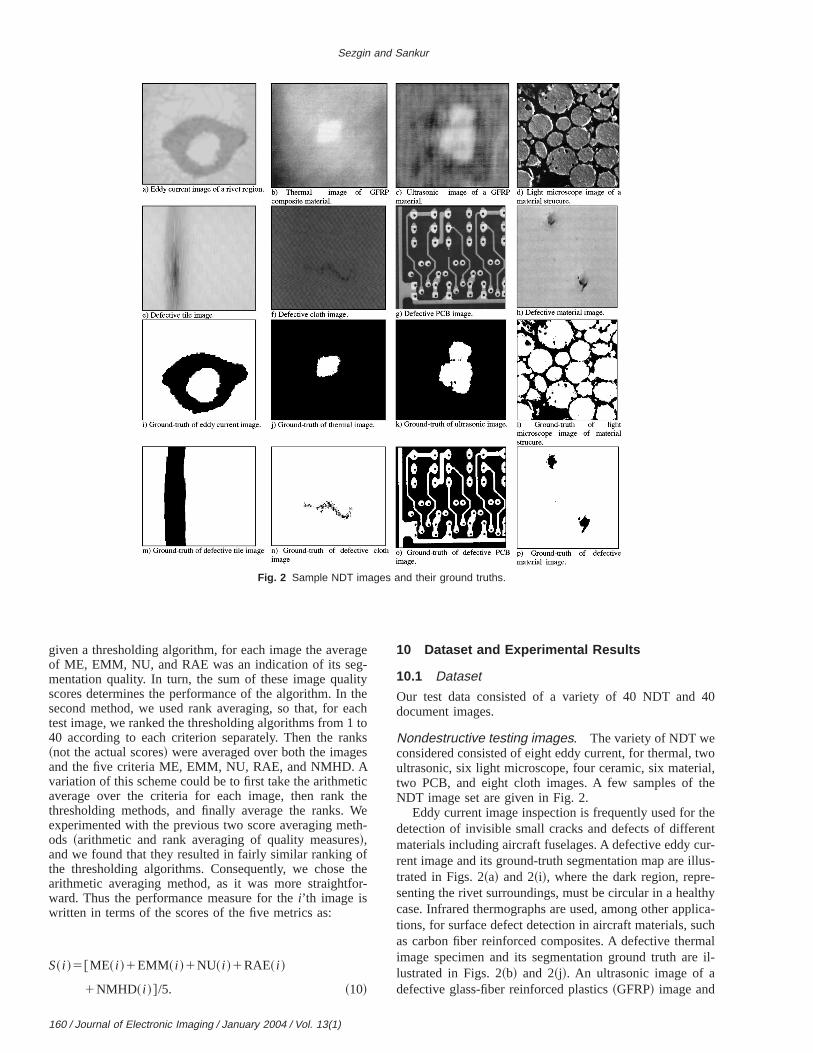
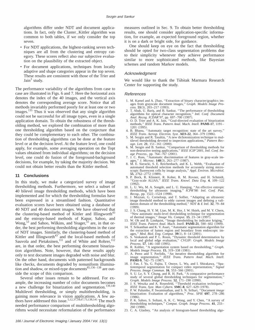
Fig. 2 Sample NDT images and their ground truths.

ag-

litythacto

nkes

tictheWethsofth

for-

40

twoal,he

thentur-lus--thylica-chalil-

given a thresholding algorithm, for each image the averof ME, EMM, NU, and RAE was an indication of its segmentation quality. In turn, the sum of these image quascores determines the performance of the algorithm. Insecond method, we used rank averaging, so that, for etest image, we ranked the thresholding algorithms from 140 according to each criterion separately. Then the ra~not the actual scores! were averaged over both the imagand the five criteria ME, EMM, NU, RAE, and NMHD. Avariation of this scheme could be to first take the arithmeaverage over the criteria for each image, then rankthresholding methods, and finally average the ranks.experimented with the previous two score averaging meods ~arithmetic and rank averaging of quality measure!,and we found that they resulted in fairly similar rankingthe thresholding algorithms. Consequently, we chosearithmetic averaging method, as it was more straightward. Thus the performance measure for thei’th image iswritten in terms of the scores of the five metrics as:

S~ i !5@ME~ i !1EMM~ i !1NU~ i !1RAE~ i !

1NMHD~ i !#/5. ~10!


e

eh

s

-

e

10 Dataset and Experimental Results

10.1 Dataset

Our test data consisted of a variety of 40 NDT anddocument images.

Nondestructive testing images. The variety of NDT weconsidered consisted of eight eddy current, for thermal,ultrasonic, six light microscope, four ceramic, six materitwo PCB, and eight cloth images. A few samples of tNDT image set are given in Fig. 2.

Eddy current image inspection is frequently used fordetection of invisible small cracks and defects of differematerials including aircraft fuselages. A defective eddy crent image and its ground-truth segmentation map are iltrated in Figs. 2~a! and 2~i!, where the dark region, representing the rivet surroundings, must be circular in a healcase. Infrared thermographs are used, among other apptions, for surface defect detection in aircraft materials, suas carbon fiber reinforced composites. A defective thermimage specimen and its segmentation ground truth arelustrated in Figs. 2~b! and 2~j!. An ultrasonic image of adefective glass-fiber reinforced plastics~GFRP! image and


Fig. 3 Sample degraded document images.

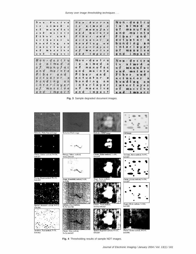
Fig. 4 Thresholding results of sample NDT images.


Sezgin and Sankur


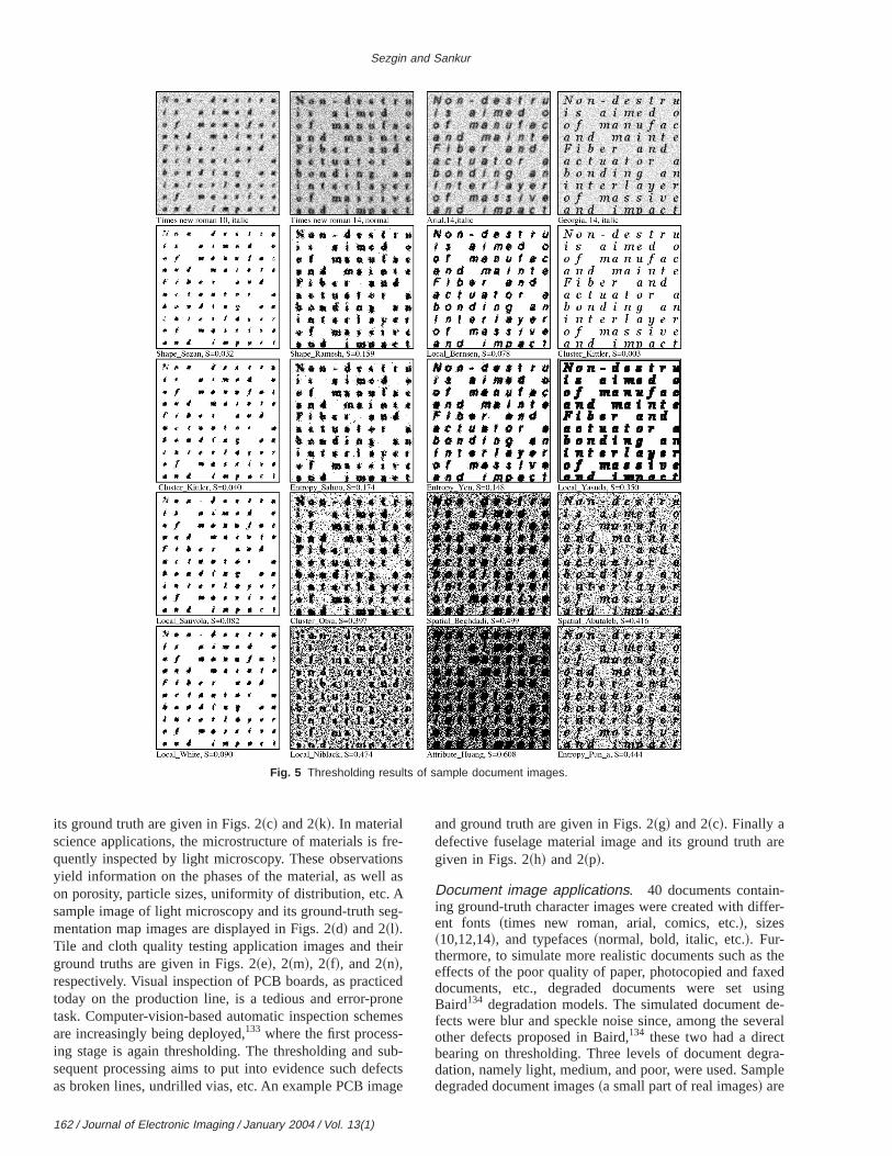
Fig. 5 Thresholding results of sample document images.

freonasAeg-

eir

cedne

me-ub

fecge

are

-er-

theedsingde-eraltra-ple

its ground truth are given in Figs. 2~c! and 2~k!. In materialscience applications, the microstructure of materials isquently inspected by light microscopy. These observatiyield information on the phases of the material, as wellon porosity, particle sizes, uniformity of distribution, etc.sample image of light microscopy and its ground-truth smentation map images are displayed in Figs. 2~d! and 2~l!.Tile and cloth quality testing application images and thground truths are given in Figs. 2~e!, 2~m!, 2~f!, and 2~n!,respectively. Visual inspection of PCB boards, as practitoday on the production line, is a tedious and error-protask. Computer-vision-based automatic inspection scheare increasingly being deployed,133 where the first processing stage is again thresholding. The thresholding and ssequent processing aims to put into evidence such deas broken lines, undrilled vias, etc. An example PCB ima


-s

s

-ts

and ground truth are given in Figs. 2~g! and 2~c!. Finally adefective fuselage material image and its ground truthgiven in Figs. 2~h! and 2~p!.

Document image applications. 40 documents containing ground-truth character images were created with diffent fonts ~times new roman, arial, comics, etc.!, sizes~10,12,14!, and typefaces~normal, bold, italic, etc.!. Fur-thermore, to simulate more realistic documents such aseffects of the poor quality of paper, photocopied and faxdocuments, etc., degraded documents were set uBaird134 degradation models. The simulated documentfects were blur and speckle noise since, among the sevother defects proposed in Baird,134 these two had a direcbearing on thresholding. Three levels of document degdation, namely light, medium, and poor, were used. Samdegraded document images~a small part of real images! are


Table 7 Thresholding evaluation ranking of 40 NDT images according to the overall average qualityscore.

Rank MethodAverage

score (AVE) Rank Method

Average

score (S)

1 Cluster–Kittler 0.256 21 Shape–Ramesh 0.460

2 Entropy–Kapur 0.261 22 Spatial–Cheng 0.481

3 Entropy–Sahoo 0.269 23 Attribute–Tsai 0.484

4 Entropy–Yen 0.289 24 Local–Bernsen 0.550

5 Cluster–Lloyd 0.292 25 Spatial–Pal–a 0.554

6 Cluster–Otsu 0.318 26 Local–Yasuda 0.573

7 Cluster–Yanni 0.328 27 Local–Palumbo 0.587

8 Local–Yanowitz 0.339 28 Entropy–Sun 0.588

9 Attribute–Hertz 0.351 29 Attribute–Leung 0.590

10 Entropy–Li 0.364 30 Entropy–Pun–a 0.591

11 Spatial–Abutaleb 0.370 31 Spatial–Beghdadi 0.619

12 Attribute–Pikaz 0.383 32 Local–Oh 0.619

13 Shape–Guo 0.391 33 Local–Niblack 0.638

14 Cluster–Ridler 0.401 34 Spatial–Pal–b 0.642

15 Cluster–Jawahar–b 0.423 35 Entropy–Pun–b 0.665

16 Attribute–Huang 0.427 36 Local–White 0.665

17 Shape–Sezan 0.431 37 Local–Kamel 0.697

18 Entropy–Shanbag 0.433 38 Local–Sauvola 0.707

19 Shape–Rosenfeld 0.442 39 Cluster–Jawahar–a 0.735

20 Shape–Olivio 0.458 40 Entropy–Brink 0.753

Table 8 Thresholding evaluation ranking of 40 degraded document images according to the overallaverage quality score.

Rank MethodAverage

score (AV) Rank Method

Average

score (S)

1 Cluster–Kittler 0.046 21 Cluster–Yanni 0.300

2 Local–Sauvola 0.066 22 Attribute–Tsai 0.308

3 Local–White 0.08 23 Attribute–Hertz 0.317

4 Local–Bernsen 0.09 24 Spatial–Cheng 0.320

5 Shape–Ramesh 0.093 25 Local–Yasuda 0.336

6 Attribute–Leung 0.110 26 Entropy–Sun 0.39

7 Entropy–Li 0.114 27 Local–Kamel 0.391

8 Cluster–Ridler 0.136 28 Entropy–Pun–a 0.463

9 Entropy–Shanbag 0.144 29 Local–Niblack 0.475

10 Shape–Sezan 0.145 30 Local–Oh 0.514

11 Entropy–Shaoo 0.148 31 Spatial–Abutaleb 0.515

12 Entropy–Kapur 0.149 32 Spatial–Pal–a 0.533

13 Entropy–Yen 0.156 33 Spatial–Beghdadi 0.539

14 Entropy–Brink 0.17 34 Attribute–Huang 0.566

15 Cluster–Lloyd 0.18 35 Entropy–Pun–b 0.593

16 Local–Palumbo 0.195 36 Shape–Guo 0.596

17 Cluster–Otsu 0.197 37 Spatial–Pal–b 0.605

18 Cluster–Jawahar–b 0.251 38 Shape–Rosenfeld 0.663

19 Attribute–Pikaz 0.259 39 Shape–Olivio 0.711

20 Local–Yanowitz 0.288 40 Cluster–Jawahar–a 0.743


Sezgin and Sankur

164 /

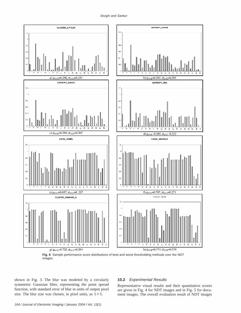
Fig. 6 Sample performance score distributions of best and worst thresholding methods over the NDTimages.

rlyeael

resu-es

shown in Fig. 3. The blur was modeled by a circulasymmetric Gaussian filter, representing the point sprfunction, with standard error of blur in units of output pixsize. The blur size was chosen, in pixel units, as 535.

Journal of Electronic Imaging / January 2004 / Vol. 13(1)

d10.2 Experimental Results

Representative visual results and their quantitative scoare given in Fig. 4 for NDT images and in Fig. 5 for docment images. The overall evaluation result of NDT imag


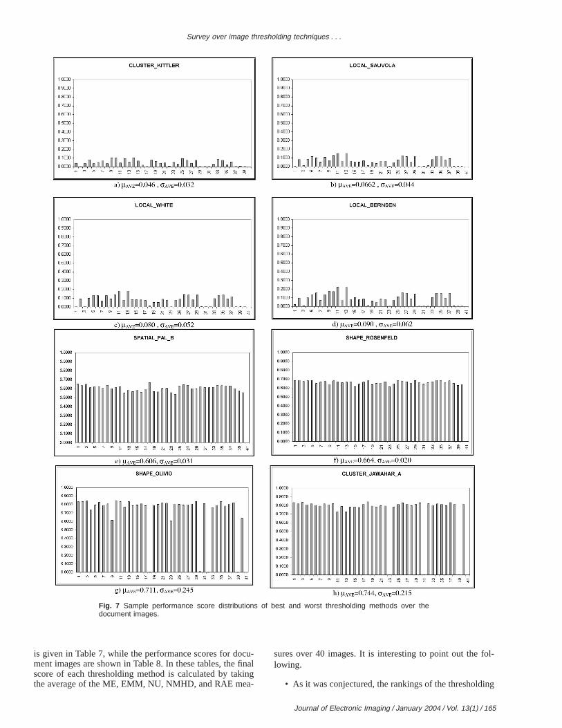
Fig. 7 Sample performance score distributions of best and worst thresholding methods over thedocument images.

cu-finaing

a-

ol-

ng

is given in Table 7, while the performance scores for doment images are shown in Table 8. In these tables, thescore of each thresholding method is calculated by takthe average of the ME, EMM, NU, NMHD, and RAE me

lsures over 40 images. It is interesting to point out the flowing.

• As it was conjectured, the rankings of the thresholdi


a-

op

ch-at-lua

llyve

and

toaxixi

t awomgleshanthainaureuldopionnde

get oenvetivsetha

an

asof

of

izaplylurnda-

eme

su-

lgoce

inga-

her

ingdueceian

-

g

n

y,’’

ul-

for

m-

ofcro-

t,

ic

nicali-

n,on

,’’

orim-

by

or

a-

cen,’’

es,’’

of

go-

Sezgin and Sankur

algorithms differ under NDT and document applictions. In fact, only the Cluster–Kittler algorithm wascommon to both tables, if we only consider the tseven.

• For NDT applications, the highest-ranking seven teniques are all from the clustering and entropy cegory. These scores reflect also our subjective evation on the plausibility of the extracted object.

• For document applications, techniques from locaadaptive and shape categories appear in the top seThese results are consistent with those of the TrierJain3 study.

The performance variability of the algorithms from casecase are illustrated in Figs. 6 and 7. Here the horizontaldenotes the index of the 40 images, and the vertical adenotes the corresponding average score. Notice thamethods invariably performed poorly for at least one or timages.135 Thus it was observed that any single algorithcould not be successful for all image types, even in a sinapplication domain. To obtain the robustness of the threolding method, we explored the combination of more thone thresholding algorithm based on the conjecturethey could be complementary to each other. The combtion of thresholding algorithms can be done at the featlevel or at the decision level. At the feature level, one coapply, for example, some averaging operation on the Tvalues obtained from individual algorithms; on the decislevel, one could do fusion of the foreground-backgroudecisions, for example, by taking the majority decision. Wcould not obtain better results than the Kittler method.

11 Conclusions

In this study, we make a categorized survey of imathresholding methods. Furthermore, we select a subse40 bilevel image thresholding methods, which have beimplemented and for which the thresholding formulas habeen expressed in a streamlined fashion. Quantitaevaluation scores have been obtained using a databa40 NDT and 40 document images. We have observedthe clustering-based method of Kittler and Illingworth43

and the entropy-based methods of Kapur, Sahoo,Wong,53 and Sahoo, Wilkins, and Yeager,55 are, in that or-der, the best performing thresholding algorithms in the cof NDT images. Similarly, the clustering-based methodKittler and Illingworth43 and the local-based methodsSauvola and Pietaksinen,111 and of White and Rohrer,112

are, in that order, the best performing document binartion algorithms. Note, however, that these results aponly to text document images degraded with noise and bOn the other hand, documents with patterned backgroulike checks, documents degraded by nonuniform illumintion and shadow, or mixed-type documents85,136–138are out-side the scope of this comparison.

Several other issues remain to be addressed. Forample, the increasing number of color documents becoa new challenge for binarization and segmentation.139,140

Multilevel thresholding, or simply multithresholding, igaining more relevance in vision applications. A few athors have addressed this issue.5,12,37,54,67,73,138,141The muchneeded performance comparison of multithresholding arithms would necessitate reformulation of the performan


-

n.

ssll

-

t-

t

f

eoft

d

e

-

.s

x-s

-

measures outlined in Sec. 9. To obtain better thresholdresults, one should consider application-specific informtion, for example, an expected foreground region, whetit is on a dark or bright side, for guidance.

One should keep on eye on the fact that thresholdshould be opted for two-class segmentation problemsto their simplicity whenever they achieve performansimilar to more sophisticated methods, like Bayesschemes and random Markov models.

Acknowledgment

We would like to thank the Tu¨bıtak Marmara ResearchCenter for supporting the study.

References

1. M. Kamel and A. Zhao, ‘‘Extraction of binary character/graphics images from grayscale document images,’’Graph. Models Image Pro-cess.55~3!, 203–217~1993!.

2. T. Abak, U. Baris¸, and B. Sankur, ‘‘The performance of thresholdinalgorithms for optical character recognition,’’Intl. Conf. DocumentAnal. Recog. ICDAR’97,pp. 697–700~1997!.

3. O. D. Trier and A. K. Jain, ‘‘Goal-directed evaluation of binarizatiomethods,’’IEEE Trans. Pattern Anal. Mach. Intell.PAMI-17 , 1191–1201 ~1995!.

4. B. Bhanu, ‘‘Automatic target recognition: state of the art surveIEEE Trans. Aerosp. Electron. Syst.AES-22, 364–379~1986!.

5. M. Sezgin and R. Tasaltin, ‘‘A new dichotomization technique to mtilevel thresholding devoted to inspection applications,’’Pattern Rec-ogn. Lett.21, 151–161~2000!.

6. M. Sezgin and B. Sankur, ‘‘Comparison of thresholding methodsnon-destructive testing applications,’’IEEE ICIP’2001, Intl. Conf. Im-age Process., pp. 764–767~2001!.

7. J. C. Russ, ‘‘Automatic discrimination of features in gray-scale iages,’’J. Microsc.148~3!, 263–277~1987!.

8. M. E. Sieracki, S. E. Reichenbach, and K. L. Webb, ‘‘Evaluationautomated threshold selection methods for accurately sizing miscopic fluorescent cells by image analysis,’’Appl. Environ. Microbiol.55, 2762–2772~1989!.

9. P. Bock, R. Klinnert, R. Kober, R. M. Rovner, and H. Schmid‘‘Gray-scale ALIAS,’’ IEEE Trans. Knowl. Data Eng.4, 109–122~1992!.

10. L. U. Wu, M. A. Songde, and L. U. Hanqing, ‘‘An effective entropthresholding for ultrasonic imaging,’’ICPR’98: Intl. Conf. Patt.Recog., pp. 1522–1524~1998!.

11. J. Moysan, G. Corneloup, and T. Sollier, ‘‘Adapting an ultrasoimage threshold method to eddy current images and defining a vdation domain of the thresholding method,’’NDT & E Intl. 32, 79–84~1999!.

12. J. S. Chang, H. Y. M. Liao, M. K. Hor, J. W. Hsieh, and M. Y. Cher‘‘New automatic multi-level thresholding technique for segmentatiof thermal images,’’Image Vis. Comput.15, 23–34~1997!.

13. W. Oh and B. Lindquist, ‘‘Image thresholding by indicator krigingIEEE Trans. Pattern Anal. Mach. Intell.PAMI-21 , 590–602~1999!.

14. T. Srikanthan and K. V. Asari, ‘‘Automatic segmentation algorithm fthe extraction of lumen region and boundary from endoscopicages,’’Med. Biol. Eng. Comput.39~1!, 8–14~2001!.

15. S. Venkatesh and P. L. Rosin, ‘‘Dynamic threshold determinationlocal and global edge evaluation,’’CVGIP: Graph. Models ImageProcess.57, 146–160~1995!.

16. R. Kohler, ‘‘A segmentation system based on thresholding,’’Graph.Models Image Process.15, 319–338~1981!.

17. A. Perez and T. Pavlidis, ‘‘An iterative thresholding algorithm fimage segmentation,’’IEEE Trans. Pattern Anal. Mach. Intell.PAMI-9 , 742–75~1987!.

18. J. Fan, J. Yu, G. Fujita, T. Onoye, L. Wu, and I. Shirakawa, ‘‘Sptiotemporal segmentation for compact video representation,’’SignalProcess. Image Commun.16, 553–566~2001!.

19. S. U. Le, S. Y. Chung, and R. H. Park, ‘‘A comparative performanstudy of several global thresholding techniques for segmentatioGraph. Models Image Process.52, 171–190~1990!.

20. J. S. Weszka and A. Rosenfeld, ‘‘Threshold evaluation techniquIEEE Trans. Syst. Man Cybern.SMC-8, 627–629~1978!.

21. P. W. Palumbo, P. Swaminathan, and S. N. Srihari, ‘‘Documentimagebinarization: Evaluation of algorithms,’’Proc. SPIE697, 278–286~1986!.

22. P. K. Sahoo, S. Soltani, A. K. C. Wong, and Y. Chen, ‘‘A surveythresholding techniques,’’Comput. Graph. Image Process.41, 233–260 ~1988!.

23. C. A. Glasbey, ‘‘An analysis of histogram-based thresholding al

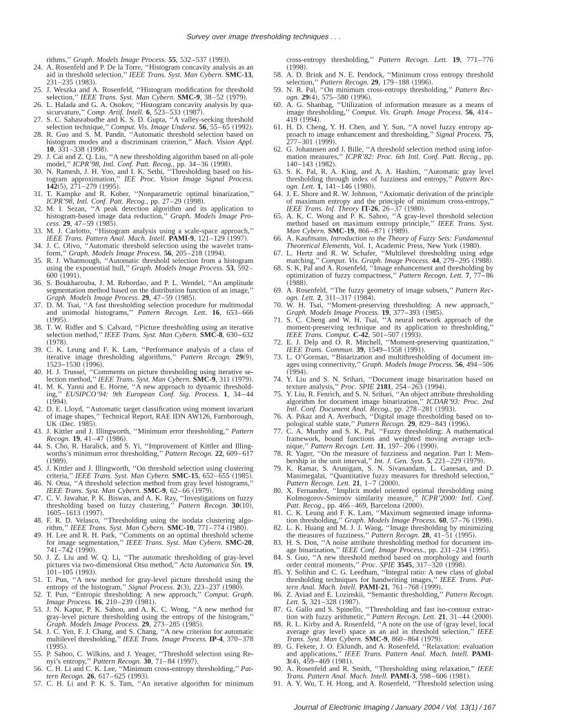
an

old

ua-

hold

on

ole

his-.

,’’

to

ch,

ns-

am

dege,’

al

ive

of

se-

ld-

ntgh,

-

ng

s,’’

zy

go-

me

el

he

or,’’

atic

Re

ld

of

p-

for-

l

pley,’’

on

tal

ge

g by

,’’

heg,’’

,’’

-

on

g

to-

alch-

em-

D.n,’’

ng

a-

g

m-

rth

al

ac-

tion

ng


rithms,’’ Graph. Models Image Process.55, 532–537~1993!.24. A. Rosenfeld and P. De la Torre, ‘‘Histogram concavity analysis as

aid in threshold selection,’’IEEE Trans. Syst. Man Cybern.SMC-13,231–235~1983!.

25. J. Weszka and A. Rosenfeld, ‘‘Histogram modification for threshselection,’’IEEE Trans. Syst. Man Cybern.SMC-9, 38–52~1979!.

26. L. Halada and G. A. Osokov, ‘‘Histogram concavity analysis by qsicurvature,’’Comp. Artif. Intell.6, 523–533~1987!.

27. S. C. Sahasrabudhe and K. S. D. Gupta, ‘‘A valley-seeking thresselection technique,’’Comput. Vis. Image Underst.56, 55–65~1992!.

28. R. Guo and S. M. Pandit, ‘‘Automatic threshold selection basedhistogram modes and a discriminant criterion,’’Mach. Vision Appl.10, 331–338~1998!.

29. J. Cai and Z. Q. Liu, ‘‘A new thresholding algorithm based on all-pmodel,’’ ICPR’98, Intl. Conf. Patt. Recog., pp. 34–36~1998!.

30. N. Ramesh, J. H. Yoo, and I. K. Sethi, ‘‘Thresholding based ontogram approximation,’’IEE Proc. Vision Image Signal Process142~5!, 271–279~1995!.

31. T. Kampke and R. Kober, ‘‘Nonparametric optimal binarizationICPR’98, Intl. Conf. Patt. Recog., pp. 27–29~1998!.

32. M. I. Sezan, ‘‘A peak detection algorithm and its applicationhistogram-based image data reduction,’’Graph. Models Image Pro-cess.29, 47–59~1985!.

33. M. J. Carlotto, ‘‘Histogram analysis using a scale-space approaIEEE Trans. Pattern Anal. Mach. Intell.PAMI-9 , 121–129~1997!.

34. J. C. Olivo, ‘‘Automatic threshold selection using the wavelet traform,’’ Graph. Models Image Process.56, 205–218~1994!.

35. R. J. Whatmough, ‘‘Automatic threshold selection from a histogrusing the exponential hull,’’Graph. Models Image Process.53, 592–600 ~1991!.

36. S. Boukharouba, J. M. Rebordao, and P. L. Wendel, ‘‘An amplitusegmentation method based on the distribution function of an imaGraph. Models Image Process.29, 47–59~1985!.

37. D. M. Tsai, ‘‘A fast thresholding selection procedure for multimodand unimodal histograms,’’Pattern Recogn. Lett.16, 653–666~1995!.

38. T. W. Ridler and S. Calvard, ‘‘Picture thresholding using an iteratselection method,’’IEEE Trans. Syst. Man Cybern.SMC-8, 630–632~1978!.

39. C. K. Leung and F. K. Lam, ‘‘Performance analysis of a classiterative image thresholding algorithms,’’Pattern Recogn.29~9!,1523–1530~1996!.

40. H. J. Trussel, ‘‘Comments on picture thresholding using iterativelection method,’’IEEE Trans. Syst. Man Cybern.SMC-9, 311~1979!.

41. M. K. Yanni and E. Horne, ‘‘A new approach to dynamic threshoing,’’ EUSIPCO’94: 9th European Conf. Sig. Process.1, 34–44~1994!.

42. D. E. Lloyd, ‘‘Automatic target classification using moment invariaof image shapes,’’ Technical Report, RAE IDN AW126, FarnborouUK ~Dec. 1985!.

43. J. Kittler and J. Illingworth, ‘‘Minimum error thresholding,’’PatternRecogn.19, 41–47~1986!.

44. S. Cho, R. Haralick, and S. Yi, ‘‘Improvement of Kittler and Illingworths’s minimum error thresholding,’’Pattern Recogn.22, 609–617~1989!.

45. J. Kittler and J. Illingworth, ‘‘On threshold selection using clustericriteria,’’ IEEE Trans. Syst. Man Cybern.SMC-15, 652–655~1985!.

46. N. Otsu, ‘‘A threshold selection method from gray level histogramIEEE Trans. Syst. Man Cybern.SMC-9, 62–66~1979!.

47. C. V. Jawahar, P. K. Biswas, and A. K. Ray, ‘‘Investigations on fuzthresholding based on fuzzy clustering,’’Pattern Recogn.30~10!,1605–1613~1997!.

48. F. R. D. Velasco, ‘‘Thresholding using the isodata clustering alrithm,’’ IEEE Trans. Syst. Man Cybern.SMC-10, 771–774~1980!.

49. H. Lee and R. H. Park, ‘‘Comments on an optimal threshold schefor image segmentation,’’IEEE Trans. Syst. Man Cybern.SMC-20,741–742~1990!.

50. J. Z. Liu and W. Q. Li, ‘‘The automatic thresholding of gray-levpictures via two-dimensional Otsu method,’’Acta Automatica Sin.19,101–105~1993!.

51. T. Pun, ‘‘A new method for gray-level picture threshold using tentropy of the histogram,’’Signal Process.2~3!, 223–237~1980!.

52. T. Pun, ‘‘Entropic thresholding: A new approach,’’Comput. Graph.Image Process.16, 210–239~1981!.

53. J. N. Kapur, P. K. Sahoo, and A. K. C. Wong, ‘‘A new method fgray-level picture thresholding using the entropy of the histogramGraph. Models Image Process.29, 273–285~1985!.

54. J. C. Yen, F. J. Chang, and S. Chang, ‘‘A new criterion for autommultilevel thresholding,’’IEEE Trans. Image Process.IP-4, 370–378~1995!.

55. P. Sahoo, C. Wilkins, and J. Yeager, ‘‘Threshold selection usingnyi’s entropy,’’ Pattern Recogn.30, 71–84~1997!.

56. C. H. Li and C. K. Lee, ‘‘Minimum cross-entropy thresholding,’’Pat-tern Recogn.26, 617–625~1993!.

57. C. H. Li and P. K. S. Tam, ‘‘An iterative algorithm for minimum

’’

’

-

cross-entropy thresholding,’’Pattern Recogn. Lett.19, 771–776~1998!.

58. A. D. Brink and N. E. Pendock, ‘‘Minimum cross entropy threshoselection,’’Pattern Recogn.29, 179–188~1996!.

59. N. R. Pal, ‘‘On minimum cross-entropy thresholding,’’Pattern Rec-ogn.29~4!, 575–580~1996!.

60. A. G. Shanbag, ‘‘Utilization of information measure as a meansimage thresholding,’’Comput. Vis. Graph. Image Process.56, 414–419 ~1994!.

61. H. D. Cheng, Y. H. Chen, and Y. Sun, ‘‘A novel fuzzy entropy aproach to image enhancement and thresholding,’’Signal Process.75,277–301~1999!.

62. G. Johannsen and J. Bille, ‘‘A threshold selection method using inmation measures,’’ICPR’82: Proc. 6th Intl. Conf. Patt. Recog., pp.140–143~1982!.

63. S. K. Pal, R. A. King, and A. A. Hashim, ‘‘Automatic gray levethresholding through index of fuzziness and entropy,’’Pattern Rec-ogn. Lett.1, 141–146~1980!.

64. J. E. Shore and R. W. Johnson, ‘‘Axiomatic derivation of the princiof maximum entropy and the principle of minimum cross-entropIEEE Trans. Inf. TheoryIT-26, 26–37~1980!.

65. A. K. C. Wong and P. K. Sahoo, ‘‘A gray-level threshold selectimethod based on maximum entropy principle,’’IEEE Trans. Syst.Man Cybern.SMC-19, 866–871~1989!.

66. A. Kaufmann,Introduction to the Theory of Fuzzy Sets: FundamenTheoretical Elements, Vol. 1, Academic Press, New York~1980!.

67. L. Hertz and R. W. Schafer, ‘‘Multilevel thresholding using edmatching,’’Comput. Vis. Graph. Image Process.44, 279–295~1988!.

68. S. K. Pal and A. Rosenfeld, ‘‘Image enhancement and thresholdinoptimization of fuzzy compactness,’’Pattern Recogn. Lett.7, 77–86~1988!.

69. A. Rosenfeld, ‘‘The fuzzy geometry of image subsets,’’Pattern Rec-ogn. Lett.2, 311–317~1984!.

70. W. H. Tsai, ‘‘Moment-preserving thresholding: A new approachGraph. Models Image Process.19, 377–393~1985!.

71. S. C. Cheng and W. H. Tsai, ‘‘A neural network approach of tmoment-preserving technique and its application to thresholdinIEEE Trans. Comput.C-42, 501–507~1993!.

72. E. J. Delp and O. R. Mitchell, ‘‘Moment-preserving quantizationIEEE Trans. Commun.39, 1549–1558~1991!.

73. L. O’Gorman, ‘‘Binarization and multithresholding of document images using connectivity,’’Graph. Models Image Process.56, 494–506~1994!.

74. Y. Liu and S. N. Srihari, ‘‘Document image binarization basedtexture analysis,’’Proc. SPIE2181, 254–263~1994!.

75. Y. Liu, R. Fenrich, and S. N. Srihari, ‘‘An object attribute thresholdinalgorithm for document image binarization,’’ICDAR’93: Proc. 2ndIntl. Conf. Document Anal. Recog., pp. 278–281~1993!.

76. A. Pikaz and A. Averbuch, ‘‘Digital image thresholding based onpological stable state,’’Pattern Recogn.29, 829–843~1996!.

77. C. A. Murthy and S. K. Pal, ‘‘Fuzzy thresholding: A mathematicframework, bound functions and weighted moving average tenique,’’ Pattern Recogn. Lett.11, 197–206~1990!.

78. R. Yager, ‘‘On the measure of fuzziness and negation. Part I: Mbership in the unit interval,’’Int. J. Gen. Syst.5, 221–229~1979!.

79. K. Ramar, S. Arunigam, S. N. Sivanandam, L. Ganesan, andManimegalai, ‘‘Quantitative fuzzy measures for threshold selectioPattern Recogn. Lett.21, 1–7 ~2000!.

80. X. Fernandez, ‘‘Implicit model oriented optimal thresholding usiKolmogorov-Smirnov similarity measure,’’ICPR’2000: Intl. Conf.Patt. Recog., pp. 466–469, Barcelona~2000!.

81. C. K. Leung and F. K. Lam, ‘‘Maximum segmented image informtion thresholding,’’Graph. Models Image Process.60, 57–76~1998!.

82. L. K. Huang and M. J. J. Wang, ‘‘Image thresholding by minimizinthe measures of fuzziness,’’Pattern Recogn.28, 41–51~1995!.

83. H. S. Don, ‘‘A noise attribute thresholding method for document iage binarization,’’IEEE Conf. Image Process., pp. 231–234~1995!.

84. S. Guo, ‘‘A new threshold method based on morphology and fouorder central moments,’’Proc. SPIE3545, 317–320~1998!.

85. Y. Solihin and C. G. Leedham, ‘‘Integral ratio: A new class of globthresholding techniques for handwriting images,’’IEEE Trans. Pat-tern Anal. Mach. Intell.PAMI-21 , 761–768~1999!.

86. Z. Aviad and E. Lozinskii, ‘‘Semantic thresholding,’’Pattern Recogn.Lett. 5, 321–328~1987!.

87. G. Gallo and S. Spinello, ‘‘Thresholding and fast iso-contour extrtion with fuzzy arithmetic,’’Pattern Recogn. Lett.21, 31–44~2000!.

88. R. L. Kirby and A. Rosenfeld, ‘‘A note on the use of~gray level, localaverage gray level! space as an aid in threshold selection,’’IEEETrans. Syst. Man Cybern.SMC-9, 860–864~1979!.

89. G. Fekete, J. O. Eklundh, and A. Rosenfeld, ‘‘Relaxation: evaluaand applications,’’IEEE Trans. Pattern Anal. Mach. Intell.PAMI-3~4!, 459–469~1981!.

90. A. Rosenfeld and R. Smith, ‘‘Thresholding using relaxation,’’IEEETrans. Pattern Anal. Mach. Intell.PAMI-3 , 598–606~1981!.

91. A. Y. Wu, T. H. Hong, and A. Rosenfeld, ‘‘Threshold selection usi


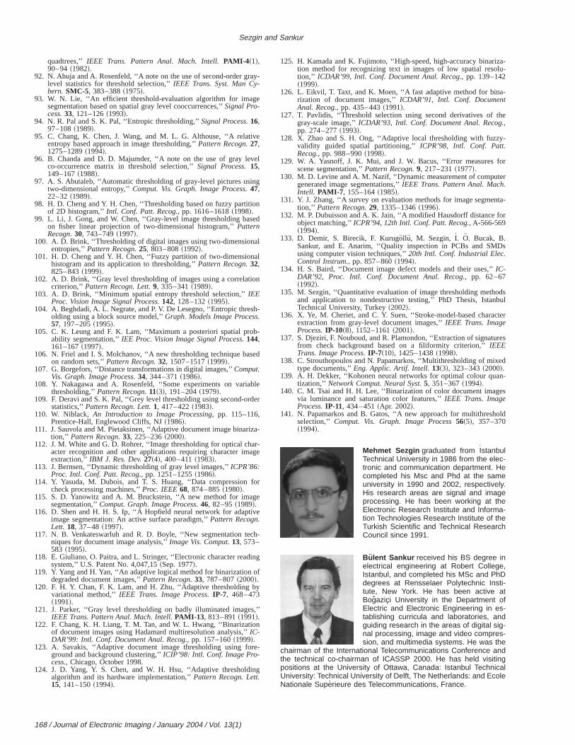
ay-

e

ve

vel

ng

ion

ed

al

al

on

sh-.

b-

ed

ble

der

iza

ar-age

for

e

ve

ch-

ing

of

by

s,’’

n

re-

ng

za-lu-

-

the.

y-

or

er

nta-

or

s

dsbul

cter

res

ed

n-

es

old

Sezgin and Sankur

quadtrees,’’ IEEE Trans. Pattern Anal. Mach. Intell.PAMI-4 ~1!,90–94~1982!.

92. N. Ahuja and A. Rosenfeld, ‘‘A note on the use of second-order grlevel statistics for threshold selection,’’IEEE Trans. Syst. Man Cy-bern.SMC-5, 383–388~1975!.

93. W. N. Lie, ‘‘An efficient threshold-evaluation algorithm for imagsegmentation based on spatial gray level cooccurrences,’’Signal Pro-cess.33, 121–126~1993!.

94. N. R. Pal and S. K. Pal, ‘‘Entropic thresholding,’’Signal Process.16,97–108~1989!.

95. C. Chang, K. Chen, J. Wang, and M. L. G. Althouse, ‘‘A relatientropy based approach in image thresholding,’’Pattern Recogn.27,1275–1289~1994!.

96. B. Chanda and D. D. Majumder, ‘‘A note on the use of gray leco-occurrence matrix in threshold selection,’’Signal Process.15,149–167~1988!.

97. A. S. Abutaleb, ‘‘Automatic thresholding of gray-level pictures usitwo-dimensional entropy,’’Comput. Vis. Graph. Image Process.47,22–32~1989!.

98. H. D. Cheng and Y. H. Chen, ‘‘Thresholding based on fuzzy partitof 2D histogram,’’Intl. Conf. Patt. Recog., pp. 1616–1618~1998!.

99. L. Li, J. Gong, and W. Chen, ‘‘Gray-level image thresholding bason fisher linear projection of two-dimensional histogram,’’PatternRecogn.30, 743–749~1997!.

100. A. D. Brink, ‘‘Thresholding of digital images using two-dimensionentropies,’’Pattern Recogn.25, 803–808~1992!.

101. H. D. Cheng and Y. H. Chen, ‘‘Fuzzy partition of two-dimensionhistogram and its application to thresholding,’’Pattern Recogn.32,825–843~1999!.

102. A. D. Brink, ‘‘Gray level thresholding of images using a correlaticriterion,’’ Pattern Recogn. Lett.9, 335–341~1989!.

103. A. D. Brink, ‘‘Minimum spatial entropy threshold selection,’’IEEProc. Vision Image Signal Process.142, 128–132~1995!.

104. A. Beghdadi, A. L. Negrate, and P. V. De Lesegno, ‘‘Entropic threolding using a block source model,’’Graph. Models Image Process57, 197–205~1995!.

105. C. K. Leung and F. K. Lam, ‘‘Maximum a posteriori spatial proability segmentation,’’IEE Proc. Vision Image Signal Process.144,161–167~1997!.

106. N. Friel and I. S. Molchanov, ‘‘A new thresholding technique bason random sets,’’Pattern Recogn.32, 1507–1517~1999!.

107. G. Borgefors, ‘‘Distance transformations in digital images,’’Comput.Vis. Graph. Image Process.34, 344–371~1986!.

108. Y. Nakagawa and A. Rosenfeld, ‘‘Some experiments on variathresholding,’’Pattern Recogn.11~3!, 191–204~1979!.

109. F. Deravi and S. K. Pal, ‘‘Grey level thresholding using second-orstatistics,’’Pattern Recogn. Lett.1, 417–422~1983!.

110. W. Niblack, An Introduction to Image Processing, pp. 115–116,Prentice-Hall, Englewood Cliffs, NJ~1986!.

111. J. Sauvola and M. Pietaksinen, ‘‘Adaptive document image binartion,’’ Pattern Recogn.33, 225–236~2000!.

112. J. M. White and G. D. Rohrer, ‘‘Image thresholding for optical chacter recognition and other applications requiring character imextraction,’’ IBM J. Res. Dev.27~4!, 400–411~1983!.

113. J. Bernsen, ‘‘Dynamic thresholding of gray level images,’’ICPR’86:Proc. Intl. Conf. Patt. Recog., pp. 1251–1255~1986!.

114. Y. Yasuda, M. Dubois, and T. S. Huang, ‘‘Data compressioncheck processing machines,’’Proc. IEEE68, 874–885~1980!.

115. S. D. Yanowitz and A. M. Bruckstein, ‘‘A new method for imagsegmentation,’’Comput. Graph. Image Process.46, 82–95~1989!.

116. D. Shen and H. H. S. Ip, ‘‘A Hopfield neural network for adaptiimage segmentation: An active surface paradigm,’’Pattern Recogn.Lett. 18, 37–48~1997!.

117. N. B. Venkateswarluh and R. D. Boyle, ‘‘New segmentation teniques for document image analysis,’’Image Vis. Comput.13, 573–583 ~1995!.

118. E. Giuliano, O. Paitra, and L. Stringer, ‘‘Electronic character readsystem,’’ U.S. Patent No. 4,047,15~Sep. 1977!.

119. Y. Yang and H. Yan, ‘‘An adaptive logical method for binarizationdegraded document images,’’Pattern Recogn.33, 787–807~2000!.

120. F. H. Y. Chan, F. K. Lam, and H. Zhu, ‘‘Adaptive thresholdingvariational method,’’IEEE Trans. Image Process.IP-7, 468–473~1991!.

121. J. Parker, ‘‘Gray level thresholding on badly illuminated imageIEEE Trans. Pattern Anal. Mach. Intell.PAMI-13 , 813–891~1991!.

122. F. Chang, K. H. Liang, T. M. Tan, and W. L. Hwang, ‘‘Binarizatioof document images using Hadamard multiresolution analysis,’’IC-DAR’99: Intl. Conf. Document Anal. Recog., pp. 157–160~1999!.

123. A. Savakis, ‘‘Adaptive document image thresholding using foground and background clustering,’’ICIP’98: Intl. Conf. Image Pro-cess., Chicago, October 1998.

124. J. D. Yang, Y. S. Chen, and W. H. Hsu, ‘‘Adaptive thresholdialgorithm and its hardware implementation,’’Pattern Recogn. Lett.15, 141–150~1994!.


-

125. H. Kamada and K. Fujimoto, ‘‘High-speed, high-accuracy binarition method for recognizing text in images of low spatial resotion,’’ ICDAR’99, Intl. Conf. Document Anal. Recog., pp. 139–142~1999!.

126. L. Eikvil, T. Taxt, and K. Moen, ‘‘A fast adaptive method for binarization of document images,’’ICDAR’91, Intl. Conf. DocumentAnal. Recog., pp. 435–443~1991!.

127. T. Pavlidis, ‘‘Threshold selection using second derivatives ofgray-scale image,’’ICDAR’93, Intl. Conf. Document Anal. Recog,pp. 274–277~1993!.

128. X. Zhao and S. H. Ong, ‘‘Adaptive local thresholding with fuzzvalidity guided spatial partitioning,’’ICPR’98, Intl. Conf. Patt.Recog., pp. 988–990~1998!.

129. W. A. Yasnoff, J. K. Mui, and J. W. Bacus, ‘‘Error measures fscene segmentation,’’Pattern Recogn.9, 217–231~1977!.

130. M. D. Levine and A. M. Nazif, ‘‘Dynamic measurement of computgenerated image segmentations,’’IEEE Trans. Pattern Anal. Mach.Intell. PAMI-7 , 155–164~1985!.

131. Y. J. Zhang, ‘‘A survey on evaluation methods for image segmetion,’’ Pattern Recogn.29, 1335–1346~1996!.

132. M. P. Dubuisson and A. K. Jain, ‘‘A modified Hausdorff distance fobject matching,’’ICPR’94, 12th Intl. Conf. Patt. Recog., A-566-569~1994!.

133. D. Demir, S. Birecik, F. Kurugo¨llu, M. Sezgin, I˙. O. Bucak, B.Sankur, and E. Anarim, ‘‘Quality inspection in PCBs and SMDusing computer vision techniques,’’20th Intl. Conf. Industrial Elec.Control Instrum., pp. 857–860~1994!.

134. H. S. Baird, ‘‘Document image defect models and their uses,’’IC-DAR’92, Proc. Intl. Conf. Document Anal. Recog., pp. 62–67~1992!.

135. M. Sezgin, ‘‘Quantitative evaluation of image thresholding methoand application to nondestructive testing,’’ PhD Thesis, IstanTechnical University, Turkey~2002!.

136. X. Ye, M. Cheriet, and C. Y. Suen, ‘‘Stroke-model-based charaextraction from gray-level document images,’’IEEE Trans. ImageProcess.IP-10~8!, 1152–1161~2001!.

137. S. Djeziri, F. Nouboud, and R. Plamondon, ‘‘Extraction of signatufrom check background based on a filiformity criterion,’’IEEETrans. Image Process.IP-7~10!, 1425–1438~1998!.

138. C. Strouthopoulos and N. Papamarkos, ‘‘Multithresholding of mixtype documents,’’Eng. Applic. Artif. Intell.13~3!, 323–343~2000!.

139. A. H. Dekker, ‘‘Kohonen neural networks for optimal colour quatization,’’ Network Comput. Neural Syst.5, 351–367~1994!.

140. C. M. Tsai and H. H. Lee, ‘‘Binarization of color document imagvia luminance and saturation color features,’’IEEE Trans. ImageProcess.IP-11, 434–451~Apr. 2002!.

141. N. Papamarkos and B. Gatos, ‘‘A new approach for multithreshselection,’’ Comput. Vis. Graph. Image Process56~5!, 357–370~1994!.

Mehmet Sezgin graduated from IstanbulTechnical University in 1986 from the elec-tronic and communication department. Hecompleted his Msc and Phd at the sameuniversity in 1990 and 2002, respectively.His research areas are signal and imageprocessing. He has been working at theElectronic Research Institute and Informa-tion Technologies Research Institute of theTurkish Scientific and Technical ResearchCouncil since 1991.

Bu lent Sankur received his BS degree inelectrical engineering at Robert College,Istanbul, and completed his MSc and PhDdegrees at Rensselaer Polytechnic Insti-tute, New York. He has been active atBogazici University in the Department ofElectric and Electronic Engineering in es-tablishing curricula and laboratories, andguiding research in the areas of digital sig-nal processing, image and video compres-sion, and multimedia systems. He was the

chairman of the International Telecommunications Conference andthe technical co-chairman of ICASSP 2000. He has held visitingpositions at the University of Ottawa, Canada: Istanbul TechnicalUniversity: Technical University of Delft, The Netherlands: and EcoleNationale Superieure des Telecommunications, France.

survey over image thresholding techniques and...

Documents