normalized iterative hard thresholding for matrix

NORMALIZED ITERATIVE HARD THRESHOLDING FOR MATRIXCOMPLETION∗

JARED TANNER† AND KE WEI‡

Abstract. Matrices of low rank can be uniquely determined from fewer linear measurements,or entries, than the total number of entries in the matrix. Moreover, there is a growing literatureof computationally efficient algorithms which can recover a low rank matrix from such limited in-formation, typically referred to as matrix completion. We introduce a particularly simple yet highlyefficient alternating projection algorithm which uses an adaptive stepsize calculated to be exact fora restricted subspace. This method is proven to have near optimal order recovery guarantees fromdense measurement masks, and is observed to have average case performance superior in some re-spects to other matrix completion algorithms for both dense measurement masks and from entrymeasurements. In particular, this proposed algorithm is able to recover matrices from extremelyclose to the minimum number of measurements necessary.

Key words. Matrix completion, compressed sensing, low-rank approximation, alternating pro-jection

AMS subject classifications. 15A29,15A83,41A29,65F10,65J20,68Q25,90C26,93C41

1. Introduction. Data with a known underlying low dimensional structure canoften be acquired from fewer measurements than simple dimension counting wouldsuggest. Moreover, there are cases where not only can the measurement process beindependent of the data, giving a linear measurement process, but the data can alsobe recovered using computationally efficient algorithms. For example, in compressedsensing [7, 11, 16], vectors of length n that have only k � n non-zero entries canoften be determined in polynomial time from less than n inner products, for detailssee [1, 3, 4, 8, 7, 10, 13, 14, 17, 18, 20, 37] and references therein. Similarly, m × nmatrices with an inherent simplicity can be uniquely determined from p < mn innerproducts. A particularly trivial example is the simplicity model of matrices with fewnon-zero entries, which can be recast as standard compressed sensing by reforming thematrix as an mn length sparse vector. Another common notion of matrix simplicityis low rank.

An m by n matrix, X ∈ Rm×n, has rank(X) = r if and only if X has a sin-gular value decomposition (SVD) X = UΣV ∗ where U and V are matrices of sizem × r and n × r respectively with orthonormal columns and Σ is a diagonal ma-trix with non-increasing and non-zero diagonal entries, σi(X) := Σ(i, i). Throughoutthis manuscript we reserve the notation U,Σ, and V to denote the singular valuedecomposition of an associated matrix. There is currently a rapidly growing liter-ature examining the acquisition of low rank matrices from what naively appears tobe an insufficient amount of information. The manifold of m × n matrices of rankr is r(m + n − r) dimensional [43], which specifies the minimum number of valuesneeded to uniquely determine such matrices; this minimal r(m + n − r) number of

∗The authors thank the Institute for Mathematics and its Applications (University of Minnesota)for their hospitality during the initial stages of this research. This work has made use of the resourcesprovided by the Edinburgh Compute and Data Facility (ECDF).

†School of Mathematics and Maxwell Institute, University of Edinburgh, Edinburgh, UK([email protected]). JT acknowledges support from the Leverhulme Trust and by the EP-SRC grant EP/J020567/1.

‡School of Mathematics and Maxwell Institute, University of Edinburgh, Edinburgh, UK([email protected]). KW acknowledges support from the China Scholarship Council.

1

2 Jared Tanner and Ke Wei

values is referred to as the oracle rate. Unfortunately the oracle rate requires theability to request entries of the singular values and vectors, which is impractical.Consider, instead, acquiring information about the low-rank matrix through p linearmeasurements of the form

b` := A(X)` = trace(A∗`X) for ` = 1, 2, · · · , p (1.1)

where the p distinct m×n matrices A` are the sensing matrices making up the operatorA(·) that maps m × n matrices to vectors of length p. The sensing matrices A` aretypically normalized such that trace(A∗

`A`) is exactly, or approximately, equal to one.Of particular interest is the case where the sensing matrices A` have only one nonzeroentry, which corresponds to directly measuring entries of X, often where the set of pmeasured entries in X are drawn uniformly at random from the

(mnp

)possible choices.

When a subset of the matrix entries are directly measured, finding the unknownentries is typically referred to as “matrix completion”, [9, 12, 25]. Recovering thedesired matrix when the measurement strategy (1.1) involves dense matrices {A`}p

`=1

lacks a widely agreed moniker; we will refer to recovery of a low rank matrix fromboth the entry sensing and dense sensing [38], as matrix completion.

This manuscript considers the question of what is an efficient algorithm capableof recovering rank r matrices with r as large as possible given p, m, n and A(·)specified. It is obvious that X is recoverable from p = mn entry measurements, asthis corresponds to directly measuring each entry in X. However, as few as r(m +n − r) measurements may be sufficient as this is the dimensionality of m × n rank rmatrices. We compare p with the maximum number of measurements required, mn,and the minimum number of measurements, r(m+n−r), through undersampling andoversampling ratios,

δ :=p

mnand ρ :=

r(m + n− r)p

(1.2)

respectively. Remarkably there are computationally efficient algorithms, such as[36, 21, 24, 22, 43, 44, 40, 5, 6, 41, 15, 33, 25, 26, 30, 45, 32, 35, 9, 12, 38, 28, 27], withthe property that if m, n, and r grow proportionally, then the smallest number of mea-surements p for which it has been proven that algorithms recover any rank r matrixgrows at most logarithmically in max(m,n) faster than the oracle rate r(m + n− r);this is referred to as near optimal order of recoverability. All of these algorithms aredesigned to return a low rank matrix that (possibly approximately) fits the measure-ments. Their efficacy is measured by both the computational speed of the algorithm,and by when they are able to return the same answer as the minimum rank problem

minX

rank(X) subject to A(X) = b. (1.3)

Although there are matrices for which (1.3) is NP-hard [23], there are computa-tionally efficient algorithms which successfully solve (1.3) for many low rank matricesencountered in practice. These algorithms can generally be classified as either directlytargeting the non-convex problem (1.3), or solving its convex-relaxation, referred toas nuclear norm minimization (NNM),

minX

‖X‖∗ :=∑

σi(X) subject to A(X) = b (1.4)

in hope that the solution of the convex-relaxation coincides with the solution of (1.3).In (1.4) the nuclear norm, ‖X‖∗, is the sum of the singular values of X, denoted

Normalized Iterative Hard Thresholding for Matrix Completion 3

σi(X). The convex-relaxation can be recast as a semidefinite program (SDP) [38]and solved using any of the algorithms designed for SDPs. Algorithms have also beendesigned to solve (1.4) specifically for matrix completion; these methods are primarilybased on iterative soft thresholding [5, 33] where the soft thesholding operator shrinksthe singular values toward zero by a specified amount, here τ ,

Sτ (X) := UΣτV ∗ where Στ (i, i) = max(0,Σ(i, i)− τ). (1.5)

Methods which directly approach the non-convex objective (1.3) are typically builtupon iterative hard thresholding [21, 24] where the hard thresholding operator setsall but a specified number of singular values to zero

Hr(X) := UΣrV∗ where Σr(i, i) :=

{Σ(i, i) i ≤ r

0 i > r.(1.6)

Note that for both soft and hard thresholding the singular values are modified, but thesingular vectors are unperturbed. Both class of algorithms have been proven to be ca-pable of recovering rank r matrices provided p ≥ Const. r(m+n−r) logα(max(m,n))for some α ≥ 0. Restricted isometry constants can be used to establish bounds of thisform, but are only applicable for Gaussian sensing and provide constants, Const., ofproportionality that are severely pessimistic.

Definition 1.1 (Restricted isometry constants (RICs), [38]). Let A(·) be a linearmap of m × n matrices to vectors of length p, Rm×n → Rp, as defined in (1.1). Forevery integer 1 ≤ r ≤ min(m,n), the restricted isometry constant, Rr, of A(·) isdefined as the smallest number such that

(1−Rr)||X||2F ≤ ||A(X)||22 ≤ (1 + Rr)||X||2F (1.7)

holds for all matrices X of rank at most r.More quantitative, non RIC based, estimates have been established for the convex-

relaxation (1.4) [39]. A notion of incoherence has also been employed to providerecovery guarantees [5] for entry sensing. Candes and Recht[9] have proven thatwith high probability, NNM (1.4) will recover the measured n × n rank r matrixprovided p ≥ Const. rn6/5 log(n); later Candes and Tao[12] sharpened this result top ≥ Const. rn log(n). Unfortunately, the incoherence approach has not given rigorousguarantees for non-convex algorithms which are the focus of this manuscript, and forthis reason we will not discuss coherence further in this manuscript.

The simplest hard thresholding algorithm for matrix completion is Iterative HardThresholding (IHT), also called Singular Value Projection [24],

Xj+1 = Hr(Xj + µjA∗(b−A(Xj))) (1.8)

where the stepsize µj is selected as a fixed constant (such as µj = 0.65 for all j), andthe adjoint of the sensing operator, A∗(·), is defined as

A∗(y) :=p∑

`=1

y(`)A` (1.9)

where the A` are the sensing matrices in (1.1). It has been shown in [24] that ifthe sensing operator A(·) satisfies R2r < 1/3 then IHT (1.8) with constant stepsizeµj = 1/(1 + R2r) is guaranteed to recover any rank r matrix; this stepsize is selected


to make the RIC based recovery condition as lax as possible, and is not advocated forimplementation as RICs are NP-hard to calculate [23] and hence are not available forthe stepsize µj . IHT has also been analysed considering a unit stepsize [21].

IHT for matrix completion is the direct extension of IHT for compressed sensing[2] where the X is a k sparse vector of length N and the sensing operator A(·) isan n × N matrix. It has been observed that IHT for compressed sensing performsdramatically better if the stepsize is selected to be optimal when the current iteratehas the same support set as the sparsest solution [3]; with this stepsize selection rulethe method is referred to as Normalized IHT (NIHT). Here we present heuristics forthe iteration dependent selection of the stepsize µj in (1.8), motivated by NIHT forcompressed sensing; we also refer to this best performing heuristic simply as NIHT,Algorithm 1, with its matrix completion context making clear its distinction fromNIHT for compressed sensing [3].

Algorithm 1 NIHT for Matrix CompletionInput: b = A(M),A, r, and termination criteriaSet X0 = Hr(A∗(b)), j = 0, and U0 as the top r left singular vectors of X0

Repeat1. Set the projection operator P j

U := UjU∗j

2. Compute the stepsize: µuj = ‖P j

UA∗(b−A(Xj))‖2F

||A(P jUA∗(b−A(Xj)))||22

3. Set Xj+1 = Hr(Xj + µujA∗(b−A(Xj)))

4. Let Uj+1 be the top r left singular vectors of Xj+1

5. j = j + 1Until termination criteria is reached ( such as ||b−A(Xj)||2 ≤ tol or j > max iter.)Output: Xj

NIHT has optimal order recovery from dense sensing, proven in Section 2.2 usinga standard RIC based proof reminiscent of [2, 3, 21, 24].

Theorem 1.2. Let A(·) : Rm×n → Rp have RIC R3r < 1/5, then NIHT willrecovery (within arbitrary precision) any rank r matrix measured by A(·).

RIC based guarantees such as Theorem 1.2 are now common for matrix comple-tion algorithms. Unfortunately such theorems lack quantitative precision sufficientto advise a practitioner as to which of the many matrix completion algorithms touse. Much more interestingly than Theorem 1.2, we observe that NIHT is extremelyefficient in a series of empirical tests, see Figures 3.3 and 3.4. For nearly all under-sampling rates δ, NIHT is able to recover matrices of larger rank than can two of thestate of the art matrix completion algorithms: NNM (1.4) and PowerFactorization(PF) [22], Algorithm 2. In particular, for δ ∈ (0.1, 1), NIHT is observed to be ableto recover matrices for nearly the largest achievable rank; that is, ρ near one. Notethat guaranteed recovery for all rank r matrices is not possible for ρ > 1/2, but thatalgorithms can recovery most low rank matrices for ρ > 1/2 [19].

Throughout this manuscript we will plot curves in the (δ, ρ) plane, below a curvethe associated algorithm is observed to typically recover the sensed matrix, and abovethe curve the algorithm is observed to typically fail to recover the sensed matrix. Werefer to these curves in the (δ, ρ) plane as phase transition curves [18]. For Gaussiansensing the phase transition for NIHT appears to oscillate with ρ between 0.85 and0.95 independent of δ and for entry sensing to slowly vary from about ρ = 0.9 atδ = 0.1 to ρ = 1 at δ = 1, see Figure 2.2. Note that ρ = 1 corresponds to achieving


the oracle minimum sampling rate of p = r(m+n−r). Moreover, for ranks where IHT(with µ = 0.65), NNM, and PF are also able to recover the sensed matrices, NIHT isobserved to be faster for entry sensing and typically faster for Gaussian sensing (1.1),see Figures 3.5 and 3.6.

The manuscript is organized as follows. In Section 2 we derive and discuss thetheory and practice of NIHT, contrasting the stepsize heuristic with constant stepsizeIHT. In Section 3 we present detailed numerical comparisons of NIHT with NNM(1.4) and PF, Algorithm 2.

2. Normalized Iterative Hard Thresholding (NIHT). Iterative algorithmsfor matrix completion are often designed by successively update a current estimateXj in order to decrease a measurement fidelity objective, such as,

‖b−A(Xj)‖22.

This is typically achieved by modifying Xj along the objective’s negative gradient

2A∗(b−A(Xj)).

For example, basic gradient descent is given by

Xj + µjA∗(b−A(Xj))

where the stepsize µj is typically selected to ensure a decrease in the objective ineach iteration. This approach can also be employed for constrained problems such as(1.3) by using alternate projection between a steepest descent update and a projectionback onto the space of rank r matrices, for a more general discussion of alternatingprojection methods see [31]. IHT (1.8) is a particularly simple example of such analternating projection method [21, 24]. Many, though not all, of the matrix com-pletion algorithms are more involved variants of projected descent methods, such as:modifying the descent direction to ensure the update remains on the manifold of rankr matrices [43, 44, 40, 35], using iterative soft thresholding (1.5) possibly with mod-ified search directions to solve (1.4) or a variant thereof [21, 5, 6, 41, 33, 25, 26, 32],and multi-stage variants [15, 30, 45] reminiscent of the compressed sensing algorithmsCoSaMP [37] and Subspace Pursuit [14]. For a recent review and empirical compari-son of many of these algorithms see [36].

The effectiveness of IHT is determined by the selection of the stepsize µj . Selectingµj too small causes the algorithm to be both slow and encourages convergence tolocal rather than the global minima, whereas selecting µj too large can result inlack of convergence. This issue has been widely discussed in the field of non-linearoptimization, including for the matrix completion algorithms discussed in [43, 44, 21,40, 35] which draw from the non-linear optimization literature. Here we consider analternative motivation drawn from compressed sensing. Large scale empirical testing[34] of a fixed stepsize for IHT in compressed sensing suggested µj = 0.65, and wefind this to also be an effective choice for a fixed stepsize for the matrix completionvariant of IHT (1.8), see Figures 3.1 and 3.2. Even more effective than the constantstepsize µj = 0.65 is the adaptive stepsize of Normalized IHT [3].

Compressed sensing and sparse approximation algorithms seek to find a (possiblyapproximate) solution to an underdetermined system of equations b = Ax with fewernonzeros than the number of rows in A. The prototypical sparse approximationalgorithm is

minx‖x‖0 subject to b = Ax (2.1)


where ‖x‖0 counts the number of non-zeros in x. As with (1.3), there are A for whichsolving (2.1) is NP-hard to solve [23]. The complication in solving (2.1) is the iden-tification of the support set of the sparsest vector; once the support set is identified,it is easy to solve for the nonzero coefficients by solving the resulting overdeterminedsystem of equations. IHT for compressed sensing is analogous to (1.8),

xj+1 = HTk(xj + µjA∗(b−Axj)),

but with HTk(·) setting all but the k largest (in magnitude) entries of the vector tobe zero and A∗ denotes the complex conjugate of A. NIHT for compressed sensingcorresponds to selecting the µj to be the optimal stepsize provided xj has identifiedthe support set of the solution to (2.1); the stepsize is given by

µj :=‖A∗

Λj (b−Axj)‖22

‖AΛj A∗Λj (b−Axj)‖2

2

where AΛj is the restriction of A to the columns corresponding to the nonzeros in xj .NIHT for matrix completion, Algorithm 1, is similarly motivated.

When IHT is converging to the minimal rank solution, each of the singular vectorsand values of the current estimate Xj must also be converging to the singular vectorsand values of the minimum rank solution. Proximity to the correct singular vectorsmotivates selecting the stepsize as if the singular vectors had been correctly identifiedand the update is being used to improve the singular values. Let the iterate Xj beof rank r with the singular value decomposition Xj = UjΣjV

∗j , then we denote the

projection onto the top r left and right singular vector spaces as

P jU := UjU

∗j (2.2)

and

P jV := VjV

∗j (2.3)

respectively. A search direction can be projected to the span of the singular vectorsby applying (2.2) from the left and (2.3) from the right; for instance, the projectednegative gradient descent direction is given by Wuv

j := P jUA∗(b − A(Xj))P j

V . Al-ternatively, a search direction can be projected to the span of just the left or rightsingular by applying only (2.2) from the left or (2.3) from the right respectively, withsearch directions given by Wu

j := P jUA∗(b − A(Xj)) and W v

j := A∗(b − A(Xj))P jV .

Using any of these restricted search directions to update the current iterate Xj resultsin the next iterate also being restricted to the same projected spaces, which wouldnot allow the iterates to converge to the lowest rank solution unless the projecteddirections had been exactly correctly identified. The analogue in compressed sensingwould be to only update the support set of the past iterate. Although the projecteddirections should not be used as the update direction, they provide useful informationfor selecting the stepsize.

The three above mentioned projected directions motivate the three stepsizes

µuj :=

‖P jUA∗(b−A(Xj))‖2

F

||A(P jUA∗(b−A(Xj)))||22

(2.4)

µvj :=

‖A∗(b−A(Xj))P jV ‖2

F

||A(A∗(b−A(Xj))P jV )||22

(2.5)

µuvj :=

‖P jUA∗(b−A(Xj))P j

V ‖2F

||A(P jUA∗(b−A(Xj))P j

V )||22. (2.6)


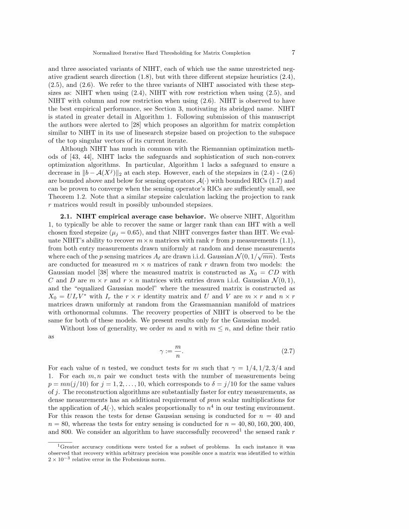
and three associated variants of NIHT, each of which use the same unrestricted neg-ative gradient search direction (1.8), but with three different stepsize heuristics (2.4),(2.5), and (2.6). We refer to the three variants of NIHT associated with these step-sizes as: NIHT when using (2.4), NIHT with row restriction when using (2.5), andNIHT with column and row restriction when using (2.6). NIHT is observed to havethe best empirical performance, see Section 3, motivating its abridged name. NIHTis stated in greater detail in Algorithm 1. Following submission of this manuscriptthe authors were alerted to [28] which proposes an algorithm for matrix completionsimilar to NIHT in its use of linesearch stepsize based on projection to the subspaceof the top singular vectors of its current iterate.

Although NIHT has much in common with the Riemannian optimization meth-ods of [43, 44], NIHT lacks the safeguards and sophistication of such non-convexoptimization algorithms. In particular, Algorithm 1 lacks a safeguard to ensure adecrease in ‖b−A(Xj)‖2 at each step. However, each of the stepsizes in (2.4) - (2.6)are bounded above and below for sensing operators A(·) with bounded RICs (1.7) andcan be proven to converge when the sensing operator’s RICs are sufficiently small, seeTheorem 1.2. Note that a similar stepsize calculation lacking the projection to rankr matrices would result in possibly unbounded stepsizes.

2.1. NIHT empirical average case behavior. We observe NIHT, Algorithm1, to typically be able to recover the same or larger rank than can IHT with a wellchosen fixed stepsize (µj = 0.65), and that NIHT converges faster than IHT. We eval-uate NIHT’s ability to recover m×n matrices with rank r from p measurements (1.1),from both entry measurements drawn uniformly at random and dense measurementswhere each of the p sensing matrices A` are drawn i.i.d. Gaussian N (0, 1/

√mn). Tests

are conducted for measured m × n matrices of rank r drawn from two models: theGaussian model [38] where the measured matrix is constructed as X0 = CD withC and D are m × r and r × n matrices with entries drawn i.i.d. Gaussian N (0, 1),and the “equalized Gaussian model” where the measured matrix is constructed asX0 = UIrV

∗ with Ir the r × r identity matrix and U and V are m × r and n × rmatrices drawn uniformly at random from the Grassmannian manifold of matriceswith orthonormal columns. The recovery properties of NIHT is observed to be thesame for both of these models. We present results only for the Gaussian model.

Without loss of generality, we order m and n with m ≤ n, and define their ratioas

γ :=m

n. (2.7)

For each value of n tested, we conduct tests for m such that γ = 1/4, 1/2, 3/4 and1. For each m,n pair we conduct tests with the number of measurements beingp = mn(j/10) for j = 1, 2, . . . , 10, which corresponds to δ = j/10 for the same valuesof j. The reconstruction algorithms are substantially faster for entry measurements, asdense measurements has an additional requirement of pmn scalar multiplications forthe application of A(·), which scales proportionally to n4 in our testing environment.For this reason the tests for dense Gaussian sensing is conducted for n = 40 andn = 80, whereas the tests for entry sensing is conducted for n = 40, 80, 160, 200, 400,and 800. We consider an algorithm to have successfully recovered1 the sensed rank r

1Greater accuracy conditions were tested for a subset of problems. In each instance it wasobserved that recovery within arbitrary precision was possible once a matrix was identified to within2× 10−3 relative error in the Frobenious norm.


matrix X0 if it returns a rank r matrix Xoutput that is within 2× 10−3 of the sensedmatrix in the relative Frobenious norm, ‖Xoutput−X0‖F ≤ 2×10−3‖X0‖F . For eachtriple m,n, p we select a value of r sufficiently small that the algorithm successfullyrecovers the sensed matrix in each of ten randomly drawn tests; we then increase therank of the sensed matrices, conducting ten tests per rank, until the rank is sufficientlylarge that the algorithm fails to recover the sense matrix in each of ten randomly drawntests. We refer to the largest value of r for which the algorithm succeeded in each often tests as rmin and the smallest value of r for which the algorithm failed in each ofthe ten tests at rmax. NIHT and IHT terminate if ‖b − A(Xj)‖2/‖b‖2 < 10−5 or ifthe multiplicative average of the last fifteen linear convergence rates are greater thanκ,

(‖b−A(Xj+15)‖2

‖b−A(Xj)‖2

)1/15

> κ. (2.8)

Unless otherwise stated we set κ = 0.999.

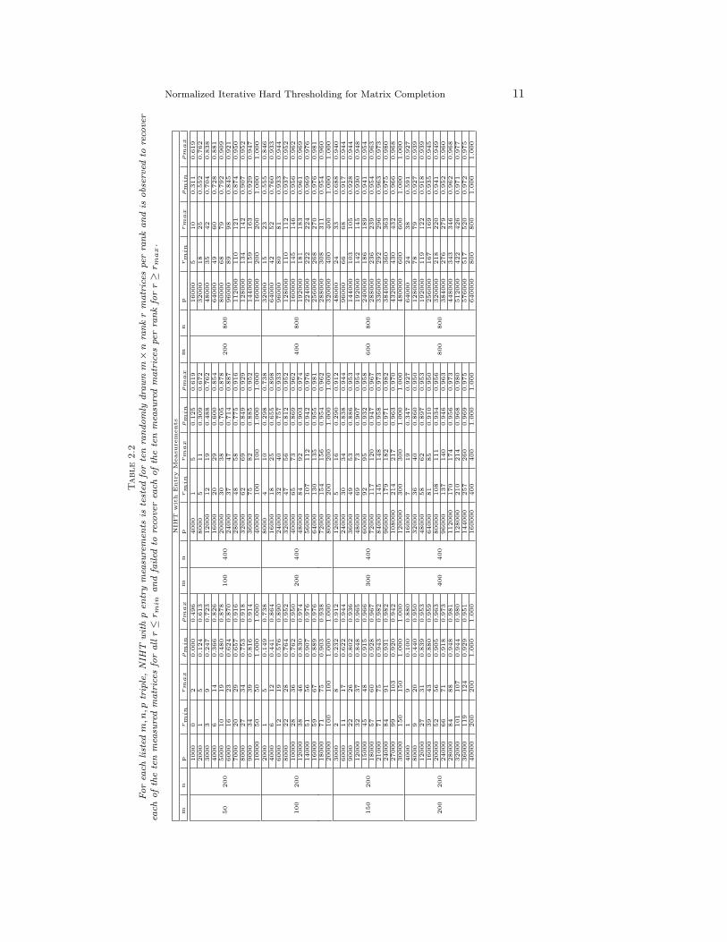
The values of rmin and rmax for NIHT, are displayed in Figure 2.1 for Gaussiansensing with n = 80 (left panel) and entry sensing with n = 800 (right panel). Thesame data is displayed in Figure 2.2, but with the vertical axis being the values of ρcalculated from (rmin +rmax)/2. The exact values of rmin, rmax and associated ρmin,and ρmax calculated from (1.2) for these, as well as smaller n, are listed in Tables 2.1and 2.2 for Gaussian sensing and entry sensing respectively.

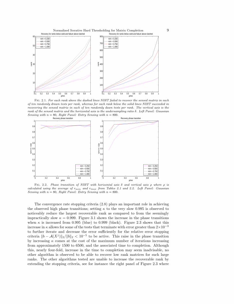
The remarkable effectiveness of NIHT is evident in Figure 2.2 through the approx-imate phase transition, calculated using (rmin+rmax)/2. Though the phase transitionfor Gaussian sensing displayed in Figure 2.2 (left panel) appears erratic due to thesmall value of n = 80 and associated large changes in ρ for a rank one change, itis surprising that the phase transitions remain between 0.85 and 0.95 for each ofγ = 1, 3/4, 1/2, and 1/4, as well as for each of δ = j/10 for j = 1, 2, . . . , 10. The phasetransition occurring between 0.85 and 0.95 indicates that irrespective of the degree ofundersampling, δ, NIHT is able to recover rank r matrices for the number of measure-ments being a small multiple of the minimum number; that is p = Const. ·r(m+n−r)for Const. < 1.2. NIHT exhibits a similarly high phase transition for entry sensingin Figure 2.2 (right panel). The entry sensing tests for the larger value of n = 800greatly reduces the sensitivity of ρ to small changes in r, resulting in much smootherobserved phase transitions. For γ = 1, 3/4, and 1/2 we observe phase transitionsthat slowly increasing from approximately ρ = 0.9 to one as δ increases from 0.2 toone. The smaller value of γ = 1/4 show substantially reduced phase transitions forentry sensing, but in Section 3 we will observe that even this lower phase transitioncompares favorably to other matrix completion algorithms. The data in Table 2.1 form = n and p = mn/10 suggest that the lower phase transition for δ = 1/10 may be anartifact of the small problem sizes. Similarly, we observe that increasing the problemsize from n = 80 to 800 results in substantial increases in the phase transitions showin Figure 3.2, including for γ = 1/4.


0.1 0.2 0.3 0.4 0.5 0.6 0.7 0.8 0.9 10

10

20

30

40

50

60

p/mn

ran

k

Recovery for ranks below solid and failure above dashed

m/n = 0.250m/n = 0.500m/n = 0.750m/n = 1.000

0.1 0.2 0.3 0.4 0.5 0.6 0.7 0.8 0.9 10

100

200

300

400

500

600

700

800

p/mnra

nk

Recovery for ranks below solid and failure above dashed

m/n = 0.250m/n = 0.500m/n = 0.750m/n = 1.000

Fig. 2.1. For each rank above the dashed lines NIHT failed to recover the sensed matrix in eachof ten randomly drawn tests per rank, whereas for each rank below the solid lines NIHT succeeded inrecovering the sensed matrix in each of ten randomly dawn tests per rank. The vertical axis is therank of the sensed matrix and the horizontal axis is the undersampling ratio δ. Left Panel: GaussianSensing with n = 80, Right Panel: Entry Sensing with n = 800.

0 0.2 0.4 0.6 0.8 10

0.1

0.2

0.3

0.4

0.5

0.6

0.7

0.8

0.9

1

p/mn

r(m

+n

−r)

/p

Recovery phase transition

m/n = 0.250m/n = 0.500m/n = 0.750m/n = 1.000

0 0.2 0.4 0.6 0.8 10

0.1

0.2

0.3

0.4

0.5

0.6

0.7

0.8

0.9

1

p/mn

r(m

+n

−r)

/p

Recovery phase transition

m/n = 0.250m/n = 0.500m/n = 0.750m/n = 1.000

Fig. 2.2. Phase transition of NIHT with horizontal axis δ and vertical axis ρ where ρ iscalculated using the average of rmin and rmax from Tables 2.1 and 2.2. Left Panel: GaussianSensing with n = 80, Right Panel: Entry Sensing with n = 800.

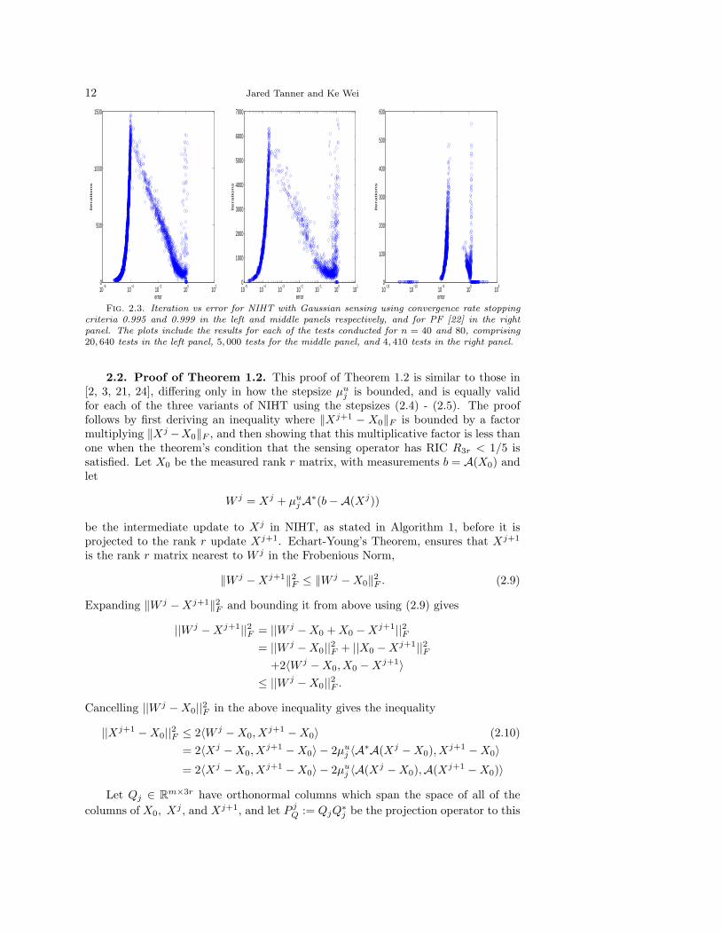
The convergence rate stopping criteria (2.8) plays an important role in achievingthe observed high phase transitions; setting κ to the very slow 0.995 is observed tonoticeably reduce the largest recoverable rank as compared to from the seeminglyimpractically slow κ = 0.999. Figure 3.1 shows the increase in the phase transitionswhen κ is increased from 0.995 (blue) to 0.999 (black). Figure 2.3 shows that thisincrease in κ allows for some of the tests that terminate with error greater than 2×10−3

to further iterate and decrease the error sufficiently for the relative error stoppingcriteria ‖b − A(Xj)‖2/‖b‖2 < 10−5 to be active. This raise in the phase transitionby increasing κ comes at the cost of the maximum number of iterations increasingfrom approximately 1500 to 6500, and the associated time to completion. Althoughthis, nearly four-fold, increase in the time to completion may seem inadvisable, noother algorithm is observed to be able to recover low rank matrices for such largeranks. The other algorithms tested are unable to increase the recoverable rank byextending the stopping criteria, see for instance the right panel of Figure 2.3 where


Table 2.1For each listed m, n, p triple, NIHT with p Gaussian measurements is tested for ten randomly

drawn m× n rank r matrices per rank and is observed to recover each of the ten measured matricesfor all r ≤ rmin and failed to recover each of the ten measured matrices per rank for r ≥ rmax.

NIHT with Gaussian Measurements

m n p rmin rmax ρmin ρmax m n p rmin rmax ρmin ρmax

10 40

40 0 0 0.000 0.000

20 80

160 1 2 0.619 1.22580 1 2 0.613 1.200 320 2 4 0.613 1.200120 2 3 0.800 1.175 480 4 5 0.800 0.990160 2 4 0.600 1.150 640 5 7 0.742 1.017200 3 5 0.705 1.125 800 7 9 0.814 1.024240 4 5 0.767 0.938 960 9 10 0.853 0.938280 5 7 0.804 1.075 1120 11 12 0.874 0.943320 6 7 0.825 0.941 1280 13 14 0.884 0.941360 7 9 0.836 1.025 1440 14 16 0.836 0.933400 8 10 0.840 1.000 1600 18 19 0.922 0.962

20 40

80 1 2 0.738 1.450

40 80

320 2 3 0.738 1.097160 2 3 0.725 1.069 640 4 6 0.725 1.069240 3 5 0.713 1.146 960 7 8 0.824 0.933320 4 6 0.700 1.012 1280 10 11 0.859 0.937400 6 7 0.810 0.927 1600 12 14 0.810 0.927480 8 9 0.867 0.956 1920 16 18 0.867 0.956560 9 11 0.820 0.963 2240 19 22 0.857 0.963640 11 13 0.842 0.955 2560 23 26 0.871 0.955720 13 15 0.849 0.938 2880 27 30 0.872 0.938800 16 18 0.880 0.945 3200 32 35 0.880 0.930

30 40

120 1 2 0.575 1.133

60 80

480 2 4 0.575 1.133240 3 4 0.838 1.100 960 6 7 0.838 0.970360 4 6 0.733 1.067 1440 9 11 0.819 0.985480 6 8 0.800 1.033 1920 13 15 0.860 0.977600 7 10 0.735 1.000 2400 17 19 0.871 0.958720 11 12 0.901 0.967 2880 21 23 0.868 0.934840 12 15 0.829 0.982 3360 26 28 0.882 0.933960 15 17 0.859 0.939 3840 32 34 0.900 0.9391080 18 21 0.867 0.953 4320 38 41 0.897 0.9401200 23 25 0.901 0.938 4800 48 49 0.920 0.929

40 40

160 1 2 0.494 0.975

80 80

640 3 4 0.736 0.975320 3 4 0.722 0.950 1280 7 8 0.837 0.950480 5 7 0.781 1.065 1920 10 12 0.781 0.925640 7 9 0.798 0.998 2560 14 17 0.798 0.950800 9 11 0.799 0.949 3200 19 22 0.837 0.949960 12 14 0.850 0.963 3840 25 27 0.879 0.9351120 15 17 0.871 0.956 4480 31 33 0.893 0.9351280 18 20 0.872 0.938 5120 37 40 0.889 0.9381440 21 24 0.860 0.933 5760 44 48 0.886 0.9331600 28 30 0.910 0.938 6400 57 59 0.917 0.931

PowerFactorization is observed to have clear separation between problem instanceswhere the algorithm converges to the sensed matrix and when it returns a low rankmatrix that differs substantially from the measured matrix.


Table

2.2

For

each

list

edm

,n,p

trip

le,N

IHT

with

pen

try

mea

sure

men

tsis

test

edfo

rte

nra

ndom

lydra

wn

m×

nra

nk

rm

atr

ices

per

rank

and

isobs

erve

dto

reco

ver

each

ofth

ete

nm

easu

red

matr

ices

for

all

r≤

r min

and

failed

tore

cove

rea

chofth

ete

nm

easu

red

matr

ices

per

rank

for

r≥

r ma

x.

NIH

Tw

ith

Entr

yM

easu

rem

ents

mn

pr

min

rm

ax

ρm

in

ρm

ax

mn

pr

min

rm

ax

ρm

in

ρm

ax

mn

pr

min

rm

ax

ρm

in

ρm

ax

50

200

1000

02

0.0

00

0.4

96

100

400

4000

15

0.1

25

0.6

19

200

800

16000

510

0.3

11

0.6

19

2000

15

0.1

24

0.6

13

8000

511

0.3

09

0.6

72

32000

18

25

0.5

52

0.7

62

3000

39

0.2

47

0.7

23

12000

12

19

0.4

88

0.7

62

48000

35

42

0.7

04

0.8

38

4000

614

0.3

66

0.8

26

16000

20

29

0.6

00

0.8

54

64000

49

60

0.7

28

0.8

81

5000

10

19

0.4

80

0.8

78

20000

30

38

0.7

05

0.8

78

80000

68

79

0.7

92

0.9

09

6000

16

23

0.6

24

0.8

70

24000

37

47

0.7

14

0.8

87

96000

89

98

0.8

45

0.9

21

7000

20

29

0.6

57

0.9

16

28000

48

58

0.7

75

0.9

16

112000

110

121

0.8

74

0.9

50

8000

27

34

0.7

53

0.9

18

32000

62

69

0.8

49

0.9

29

128000

134

142

0.9

07

0.9

52

9000

34

39

0.8

16

0.9

14

36000

75

82

0.8

85

0.9

52

144000

159

163

0.9

29

0.9

47

10000

50

50

1.0

00

1.0

00

40000

100

100

1.0

00

1.0

00

160000

200

200

1.0

00

1.0

00

100

200

2000

15

0.1

49

0.7

38

200

400

8000

410

0.2

98

0.7

38

400

800

32000

15

23

0.5

55

0.8

46

4000

612

0.4

41

0.8

64

16000

18

25

0.6

55

0.8

98

64000

42

52

0.7

60

0.9

33

6000

12

19

0.5

76

0.8

90

24000

32

40

0.7

57

0.9

33

96000

80

81

0.9

33

0.9

44

8000

22

28

0.7

64

0.9

52

32000

47

56

0.8

12

0.9

52

128000

110

112

0.9

37

0.9

52

10000

28

36

0.7

62

0.9

50

40000

65

73

0.8

69

0.9

62

160000

145

146

0.9

56

0.9

62

12000

38

46

0.8

30

0.9

74

48000

84

92

0.9

03

0.9

74

192000

181

183

0.9

61

0.9

69

14000

51

56

0.9

07

0.9

76

56000

107

112

0.9

42

0.9

76

224000

222

224

0.9

69

0.9

76

16000

59

67

0.8

89

0.9

76

64000

130

135

0.9

55

0.9

81

256000

268

270

0.9

76

0.9

81

18000

71

75

0.9

03

0.9

38

72000

154

156

0.9

54

0.9

62

288000

308

311

0.9

54

0.9

60

20000

100

100

1.0

00

1.0

00

80000

200

200

1.0

00

1.0

00

320000

400

400

1.0

00

1.0

00

150

200

3000

28

0.2

32

0.9

12

300

400

12000

516

0.2

90

0.9

12

600

800

48000

24

33

0.6

88

0.9

40

6000

11

17

0.6

22

0.9

44

24000

30

34

0.8

38

0.9

44

96000

66

68

0.9

17

0.9

44

9000

22

26

0.8

02

0.9

36

36000

49

53

0.8

86

0.9

53

144000

103

105

0.9

28

0.9

44

12000

32

37

0.8

48

0.9

65

48000

69

73

0.9

07

0.9

54

192000

142

145

0.9

30

0.9

48

15000

45

48

0.9

15

0.9

66

60000

92

95

0.9

32

0.9

58

240000

186

189

0.9

41

0.9

54

18000

57

60

0.9

28

0.9

67

72000

117

120

0.9

47

0.9

67

288000

236

239

0.9

54

0.9

63

21000

71

75

0.9

43

0.9

82

84000

145

148

0.9

58

0.9

73

336000

292

296

0.9

63

0.9

73

24000

84

91

0.9

31

0.9

82

96000

179

182

0.9

71

0.9

82

384000

360

363

0.9

75

0.9

80

27000

99

103

0.9

20

0.9

42

108000

214

217

0.9

63

0.9

70

432000

430

432

0.9

66

0.9

68

30000

150

150

1.0

00

1.0

00

120000

300

300

1.0

00

1.0

00

480000

600

600

1.0

00

1.0

00

200

200

4000

19

0.1

00

0.8

80

400

400

16000

719

0.3

47

0.9

27

800

800

64000

24

38

0.5

91

0.9

27

8000

920

0.4

40

0.9

50

32000

36

40

0.8

60

0.9

50

128000

78

79

0.9

27

0.9

39

12000

27

31

0.8

39

0.9

53

48000

58

62

0.8

97

0.9

53

192000

119

122

0.9

18

0.9

39

16000

39

43

0.8

80

0.9

59

64000

81

85

0.9

10

0.9

50

256000

167

169

0.9

35

0.9

45

20000

52

56

0.9

05

0.9

63

80000

108

111

0.9

34

0.9

56

320000

218

220

0.9

41

0.9

49

24000

66

71

0.9

18

0.9

73

96000

137

140

0.9

46

0.9

63

384000

276

279

0.9

52

0.9

60

28000

84

88

0.9

48

0.9

81

112000

170

174

0.9

56

0.9

73

448000

343

346

0.9

62

0.9

68

32000

101

107

0.9

44

0.9

80

128000

210

214

0.9

68

0.9

80

512000

422

426

0.9

71

0.9

77

36000

119

124

0.9

29

0.9

51

144000

257

260

0.9

69

0.9

75

576000

517

520

0.9

72

0.9

75

40000

200

200

1.0

00

1.0

00

160000

400

400

1.0

00

1.0

00

640000

800

800

1.0

00

1.0

00


10−6

10−4

10−2

100

102

0

500

1000

1500

error

ite

ra

tio

ns

10−5

10−4

10−3

10−2

10−1

100

101

0

1000

2000

3000

4000

5000

6000

7000

error

ite

ra

tio

ns

10−15

10−10

10−5

100

105

0

100

200

300

400

500

600

error

ite

ra

tio

ns

Fig. 2.3. Iteration vs error for NIHT with Gaussian sensing using convergence rate stoppingcriteria 0.995 and 0.999 in the left and middle panels respectively, and for PF [22] in the rightpanel. The plots include the results for each of the tests conducted for n = 40 and 80, comprising20, 640 tests in the left panel, 5, 000 tests for the middle panel, and 4, 410 tests in the right panel.

2.2. Proof of Theorem 1.2. This proof of Theorem 1.2 is similar to those in[2, 3, 21, 24], differing only in how the stepsize µu

j is bounded, and is equally validfor each of the three variants of NIHT using the stepsizes (2.4) - (2.5). The prooffollows by first deriving an inequality where ‖Xj+1 − X0‖F is bounded by a factormultiplying ‖Xj −X0‖F , and then showing that this multiplicative factor is less thanone when the theorem’s condition that the sensing operator has RIC R3r < 1/5 issatisfied. Let X0 be the measured rank r matrix, with measurements b = A(X0) andlet

W j = Xj + µujA∗(b−A(Xj))

be the intermediate update to Xj in NIHT, as stated in Algorithm 1, before it isprojected to the rank r update Xj+1. Echart-Young’s Theorem, ensures that Xj+1

is the rank r matrix nearest to W j in the Frobenious Norm,

‖W j −Xj+1‖2F ≤ ‖W j −X0‖2

F . (2.9)

Expanding ‖W j −Xj+1‖2F and bounding it from above using (2.9) gives

||W j −Xj+1||2F = ||W j −X0 + X0 −Xj+1||2F= ||W j −X0||2F + ||X0 −Xj+1||2F

+2〈W j −X0, X0 −Xj+1〉≤ ||W j −X0||2F .

Cancelling ||W j −X0||2F in the above inequality gives the inequality

||Xj+1 −X0||2F ≤ 2〈W j −X0, Xj+1 −X0〉 (2.10)

= 2〈Xj −X0, Xj+1 −X0〉 − 2µu

j 〈A∗A(Xj −X0), Xj+1 −X0〉= 2〈Xj −X0, X

j+1 −X0〉 − 2µuj 〈A(Xj −X0),A(Xj+1 −X0)〉

Let Qj ∈ Rm×3r have orthonormal columns which span the space of all of thecolumns of X0, Xj , and Xj+1, and let P j

Q := QjQ∗j be the projection operator to this


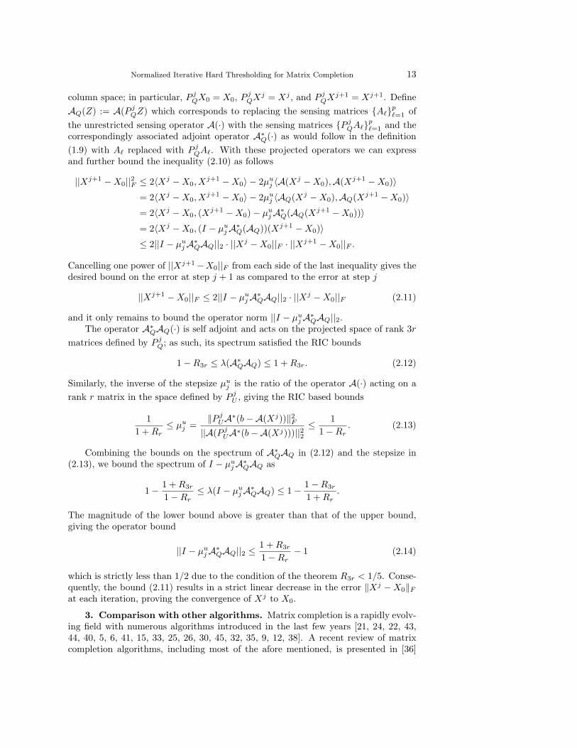
column space; in particular, P jQX0 = X0, P j

QXj = Xj , and P jQXj+1 = Xj+1. Define

AQ(Z) := A(P jQZ) which corresponds to replacing the sensing matrices {A`}p

`=1 ofthe unrestricted sensing operator A(·) with the sensing matrices {P j

QA`}p`=1 and the

correspondingly associated adjoint operator A∗Q(·) as would follow in the definition

(1.9) with A` replaced with P jQA`. With these projected operators we can express

and further bound the inequality (2.10) as follows

||Xj+1 −X0||2F ≤ 2〈Xj −X0, Xj+1 −X0〉 − 2µu

j 〈A(Xj −X0),A(Xj+1 −X0)〉= 2〈Xj −X0, X

j+1 −X0〉 − 2µuj 〈AQ(Xj −X0),AQ(Xj+1 −X0)〉

= 2〈Xj −X0, (Xj+1 −X0)− µujA∗

Q(AQ(Xj+1 −X0))〉= 2〈Xj −X0, (I − µu

jA∗Q(AQ))(Xj+1 −X0)〉

≤ 2||I − µujA∗

QAQ||2 · ||Xj −X0||F · ||Xj+1 −X0||F .

Cancelling one power of ||Xj+1−X0||F from each side of the last inequality gives thedesired bound on the error at step j + 1 as compared to the error at step j

||Xj+1 −X0||F ≤ 2||I − µujA∗

QAQ||2 · ||Xj −X0||F (2.11)

and it only remains to bound the operator norm ||I − µujA∗

QAQ||2.The operator A∗

QAQ(·) is self adjoint and acts on the projected space of rank 3r

matrices defined by P jQ; as such, its spectrum satisfied the RIC bounds

1−R3r ≤ λ(A∗QAQ) ≤ 1 + R3r. (2.12)

Similarly, the inverse of the stepsize µuj is the ratio of the operator A(·) acting on a

rank r matrix in the space defined by P jU , giving the RIC based bounds

11 + Rr

≤ µuj =

‖P jUA∗(b−A(Xj))‖2

F

||A(P jUA∗(b−A(Xj)))||22

≤ 11−Rr

. (2.13)

Combining the bounds on the spectrum of A∗QAQ in (2.12) and the stepsize in

(2.13), we bound the spectrum of I − µujA∗

QAQ as

1− 1 + R3r

1−Rr≤ λ(I − µu

jA∗QAQ) ≤ 1− 1−R3r

1 + Rr.

The magnitude of the lower bound above is greater than that of the upper bound,giving the operator bound

||I − µujA∗

QAQ||2 ≤1 + R3r

1−Rr− 1 (2.14)

which is strictly less than 1/2 due to the condition of the theorem R3r < 1/5. Conse-quently, the bound (2.11) results in a strict linear decrease in the error ‖Xj −X0‖F

at each iteration, proving the convergence of Xj to X0.

3. Comparison with other algorithms. Matrix completion is a rapidly evolv-ing field with numerous algorithms introduced in the last few years [21, 24, 22, 43,44, 40, 5, 6, 41, 15, 33, 25, 26, 30, 45, 32, 35, 9, 12, 38]. A recent review of matrixcompletion algorithms, including most of the afore mentioned, is presented in [36]


along with extensive numerical comparisons. The focus of the numerical tests pre-sented here is on quantifying the largest possible rank recoverable for an algorithmas a function of p/mn, and to explore if this phase transition is stable as the matrixsize increases. This testing environment probes algorithms in the region where theirconvergence rates slow, causing the tests to have an unusually high computationalburden. The tests presented in this manuscript required 4.67 CPU years2 run on hexcore Intel X5650 CPUs with 24 GB of RAM.

The empirical behavior of NIHT has been presented in Section 2.1. Here wecontrast the performance of NIHT with: fixed stepsize IHT (µj = 0.65), NNM using asemidefinite programming formulation [38] and the software package SDPT3 [42], andPF [22], Algorithm 2. These three algorithms are selected as representative examples

Algorithm 2 PowerFactorization (PF) for Matrix CompletionInput: U0 ∈ Rm×r, V 0 ∈ Rr×n

Repeat1. Hold V j−1 fixed, solve U j = arg min

U||A(UV j−1)− b||2

2. Hold U j fixed, solve V j = arg minV ||A(U jV )− b||23. j = j + 1

Until some criteria meetsOuput Xj = U jV j

of hard thresholding algorithms, IHT, convex relaxations, NNM, and a quite distinctvariant of optimization on the manifold of low rank matrices, PF. PF was selected dueto both its simplicity and its remarkably high phase transition [22]. The primary focusof this comparison is to determine of the largest rank recoverable by an algorithm fora given m,n, p triple. Timings are included for completeness. Each algorithm is testedas described in the first paragraph of Section 2.1.

3.1. Comparison of IHT and NIHT. We consider (1.8) with four stepsizechoices, IHT with fixed stepsize µj = 0.65 as well as three variants of NIHT with it-eration adaptive stepsizes as stated in (2.4) - (2.6). The RIC based analysis of NIHTwith stepsize (2.4) presented in Section 2.2 is equally valid for stepsizes (2.5) and (2.6).Unfortunately, this worst case analysis gives little indication of their average case effec-tiveness. Tests were conducted for matrices with aspect ratio m/n = 1, 3/4, 1/2, 1/4,and 1/8 for n = 40 and n = 80. The variant with stepsize (2.5) was able to recovermatrices of the same rank as (2.4) when m/n = 1, 3/4, and 1/2, but was only ableto recover substantially lower rank matrices for the more rectangular aspect ratiosm/n = 1/4 and 1/8. The NIHT variant with stepsize (2.6) was able to only recovermatrices of greatly reduced rank as compared to (2.4) and (2.5). For conciseness welimit ourselves to presenting only the results for the adaptive stepsize variant (2.4),which we refer to simply as NIHT and state in greater detail as Algorithm 1.

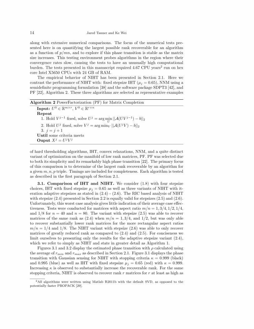
Figures 3.1 and 3.2 display the estimated phase transition with ρ calculated usingthe average of rmin and rmax as described in Section 2.1. Figure 3.1 displays the phasetransition with Gaussian sensing for NIHT with stopping criteria κ = 0.999 (black)and 0.995 (blue) as well as IHT with fixed stepsize µj = 0.65 (red) with κ = 0.999.Increasing κ is observed to substantially increase the recoverable rank. For the samestopping criteria, NIHT is observed to recover rank r matrices for r at least as high as

2All algorithms were written using Matlab R2011b with the default SVD, as opposed to thepotentially faster PROPACK [29].


0 0.2 0.4 0.6 0.8 10

0.1

0.2

0.3

0.4

0.5

0.6

0.7

0.8

0.9

1

p/mn

r(m

+n

−r)

/pRecovery phase transition with m/n = 1.000

NIHT: Column Projection (0.999) with Gaussian MeasurementsIHT: stepsize=0.65 (0.999) with Gaussian MeasurementsNIHT: Column Projection (0.995) with Gaussian Measurements

0 0.2 0.4 0.6 0.8 10

0.1

0.2

0.3

0.4

0.5

0.6

0.7

0.8

0.9

1

p/mn

r(m

+n

−r)

/p

Recovery phase transition with m/n = 0.750


(a) (b)

0 0.2 0.4 0.6 0.8 10

0.1

0.2

0.3

0.4

0.5

0.6

0.7

0.8

0.9

1

p/mn

r(m

+n

−r)

/p



0 0.2 0.4 0.6 0.8 10

0.1

0.2

0.3

0.4

0.5

0.6

0.7

0.8

0.9

1

p/mn

r(m

+n

−r)

/p



(c) (d)

Fig. 3.1. Phase transition for Gaussian Sensing and algorithms: NIHT with stopping criteriaκ = 0.999 and κ = 0.995 as well as IHT with stepsize µj = 0.65 and stopping criteria κ = 0.999.Horizontal axis δ and vertical axis ρ as defined in (1.2). Each transition is for n = 80 and thevalues of ρ shown are calculated using the average of rmin and rmax.

IHT. The average timings for the associated tests with κ = 0.999 and m = n = 40 aredisplayed in Figure 3.5 Panels (b) and (d) for NIHT and IHT respectively, and theratio of their average timings is displayed in Figure 3.6 Panel (b). NIHT is observedto be faster than IHT except for the region of large δ and ρ where IHT is beginningto fail to recover the solution to (1.3) but NIHT remains able to recover the solutionto (1.3).

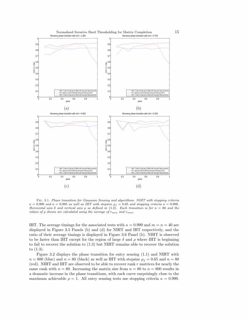
Figure 3.2 displays the phase transition for entry sensing (1.1) and NIHT withn = 800 (blue) and n = 80 (black) as well as IHT with stepsize µj = 0.65 and n = 80(red). NIHT and IHT are observed to be able to recover rank r matrices for nearly thesame rank with n = 80. Increasing the matrix size from n = 80 to n = 800 results ina dramatic increase in the phase transitions, with each curve surprisingly close to themaximum achievable ρ = 1. All entry sensing tests use stopping criteria κ = 0.999.


0 0.2 0.4 0.6 0.8 10

0.1

0.2

0.3

0.4

0.5

0.6

0.7

0.8

0.9

1

p/mn

r(m

+n

−r)


NIHT: Column Projection (0.999) with Entry MeasurementsIHT: stepsize=0.65 (0.999) with Entry MeasurementsNIHT: Column Projection (0.999) with Entry Measurements

0 0.2 0.4 0.6 0.8 10

0.1

0.2

0.3

0.4

0.5

0.6

0.7

0.8

0.9

1

p/mn

r(m

+n

−r)

/p



(a) (b)

0 0.2 0.4 0.6 0.8 10

0.1

0.2

0.3

0.4

0.5

0.6

0.7

0.8

0.9

1

p/mn

r(m

+n

−r)

/p



0 0.2 0.4 0.6 0.8 10

0.1

0.2

0.3

0.4

0.5

0.6

0.7

0.8

0.9

1

p/mn

r(m

+n

−r)

/p



(c) (d)

Fig. 3.2. Phase transition for entry sensing and algorithms: NIHT with column projection forn = 80 (black) and n = 800 (blue) and IHT with stepsize µj = 0.65 (red) with n = 80. Horizontalaxis δ and vertical axis ρ as defined in (1.2). The values of ρ shown are calculated using the averageof rmin and rmax.

The average timings for the associated tests with n = m = 80 are displayed in Figure3.5 Panels (a) and (c) for NIHT and IHT respectively, and the ratio of their averagetimings is displayed in Figure 3.6 Panel (a). NIHT is observed to always be fasterthan IHT, typically taking just under half the time.

3.2. Comparison of NIHT with Nuclear Norm Minimization and PowerFactorization. Nuclear norm minimization (NNM), (1.4), is the convex relaxationof the rank minimization question (1.3), and is the most studied approach for matrixcompletion [9, 12, 38]. In particular, it is the only matrix completion formulationwith a quantitatively accurate analysis [39] of the ability to recover the solution to(1.3). Having a formulation in terms of the well studied semidefinite programming,there are many existing algorithms and software packages that can be used to solve


(1.4); moreover, numerous algorithms have been designed to solve NNM specificallyfor matrix completion, [5, 6, 41, 33] to name a few. These matrix completion focusedmethods for the solution of (1.4) are designed to more accurately and/or more rapidlyreturn the solution, but remain designed to give the solution to (1.4) and do not in-crease the range of the parameters δ and ρ where the solution to (1.4) correspondsto that of (1.3). With our focus of determining the largest recoverable rank for analgorithm, we use the well established software package SDPT3 [42], but are awarethat specialized software is likely able to solve (1.4) in substantially less time. In ad-dition to contrasting NIHT with NNM, we also compare NIHT with the very differentmanifold optimization method PowerFactorization (PF) [22], see Algorithm 2.

PF seeks to directly solve the minimum rank problem (1.3) and is a particularlysimple example of a class of methods [26, 45, 35] which are designed to remain on themanifold of rank r matrices throughout each iteration. Despite its simplicity, PF iscapable of recovering matrices of surprisingly large rank. In contrast, NIHT updatesthe solution with directions that result in intermediate updates which are not on themanifold of rank r matrices; the algorithms presented in [43, 44, 28, 27, 40] are similarto NIHT in their use of (possibly restricted) descent directions of the measurementresidual followed by projection onto the manifold of rank r matrices.

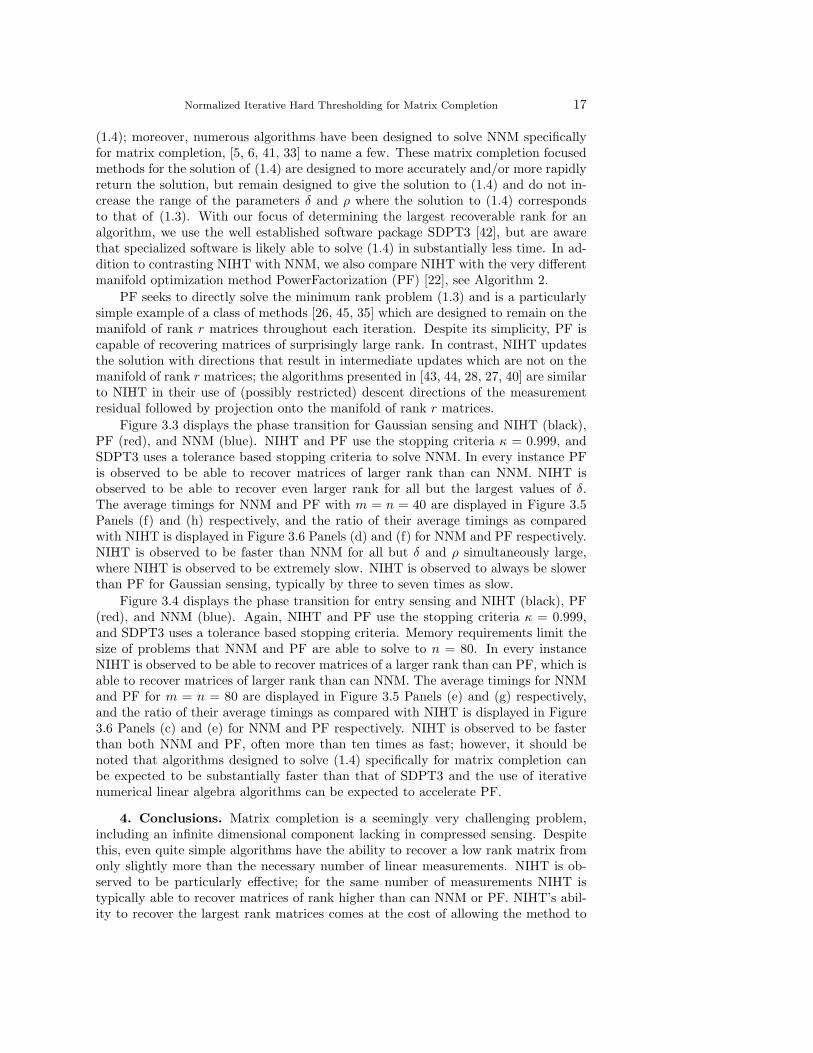
Figure 3.3 displays the phase transition for Gaussian sensing and NIHT (black),PF (red), and NNM (blue). NIHT and PF use the stopping criteria κ = 0.999, andSDPT3 uses a tolerance based stopping criteria to solve NNM. In every instance PFis observed to be able to recover matrices of larger rank than can NNM. NIHT isobserved to be able to recover even larger rank for all but the largest values of δ.The average timings for NNM and PF with m = n = 40 are displayed in Figure 3.5Panels (f) and (h) respectively, and the ratio of their average timings as comparedwith NIHT is displayed in Figure 3.6 Panels (d) and (f) for NNM and PF respectively.NIHT is observed to be faster than NNM for all but δ and ρ simultaneously large,where NIHT is observed to be extremely slow. NIHT is observed to always be slowerthan PF for Gaussian sensing, typically by three to seven times as slow.

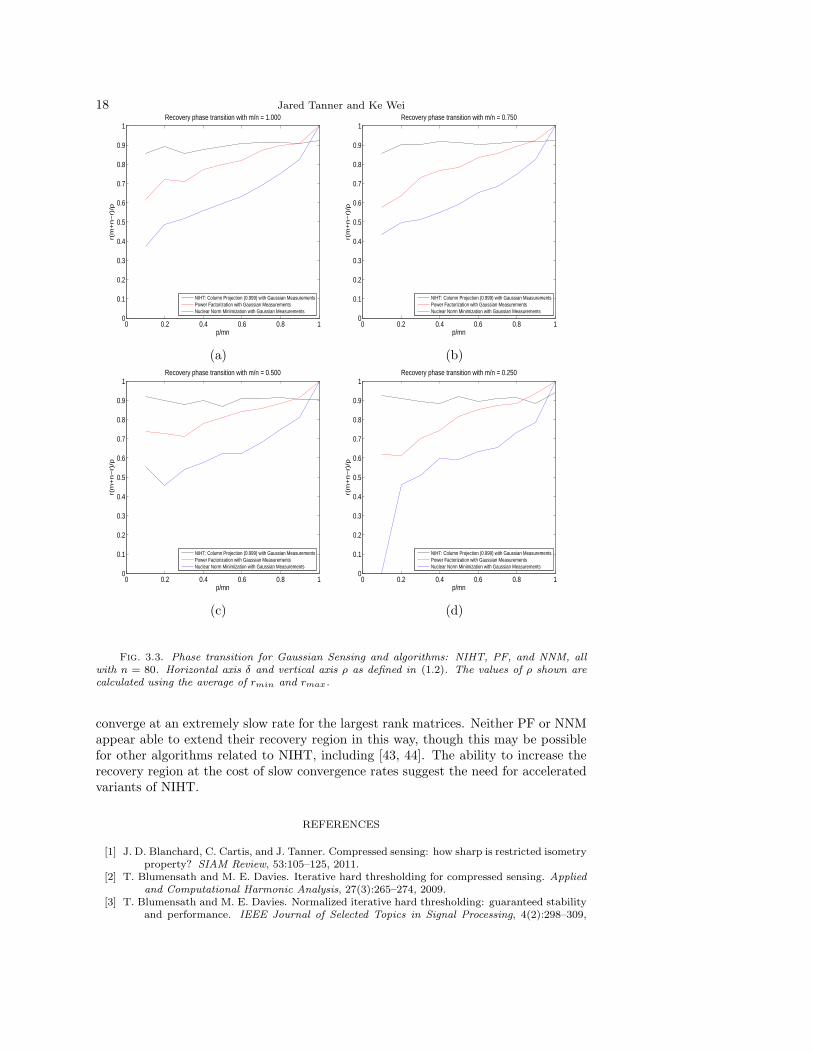
Figure 3.4 displays the phase transition for entry sensing and NIHT (black), PF(red), and NNM (blue). Again, NIHT and PF use the stopping criteria κ = 0.999,and SDPT3 uses a tolerance based stopping criteria. Memory requirements limit thesize of problems that NNM and PF are able to solve to n = 80. In every instanceNIHT is observed to be able to recover matrices of a larger rank than can PF, which isable to recover matrices of larger rank than can NNM. The average timings for NNMand PF for m = n = 80 are displayed in Figure 3.5 Panels (e) and (g) respectively,and the ratio of their average timings as compared with NIHT is displayed in Figure3.6 Panels (c) and (e) for NNM and PF respectively. NIHT is observed to be fasterthan both NNM and PF, often more than ten times as fast; however, it should benoted that algorithms designed to solve (1.4) specifically for matrix completion canbe expected to be substantially faster than that of SDPT3 and the use of iterativenumerical linear algebra algorithms can be expected to accelerate PF.

4. Conclusions. Matrix completion is a seemingly very challenging problem,including an infinite dimensional component lacking in compressed sensing. Despitethis, even quite simple algorithms have the ability to recover a low rank matrix fromonly slightly more than the necessary number of linear measurements. NIHT is ob-served to be particularly effective; for the same number of measurements NIHT istypically able to recover matrices of rank higher than can NNM or PF. NIHT’s abil-ity to recover the largest rank matrices comes at the cost of allowing the method to


0 0.2 0.4 0.6 0.8 10

0.1

0.2

0.3

0.4

0.5

0.6

0.7

0.8

0.9

1

p/mn

r(m

+n

−r)


NIHT: Column Projection (0.999) with Gaussian MeasurementsPower Factorization with Gaussian MeasurementsNuclear Norm Minimization with Gaussian Measurements

0 0.2 0.4 0.6 0.8 10

0.1

0.2

0.3

0.4

0.5

0.6

0.7

0.8

0.9

1

p/mn

r(m

+n

−r)

/p



(a) (b)

0 0.2 0.4 0.6 0.8 10

0.1

0.2

0.3

0.4

0.5

0.6

0.7

0.8

0.9

1

p/mn

r(m

+n

−r)

/p



0 0.2 0.4 0.6 0.8 10

0.1

0.2

0.3

0.4

0.5

0.6

0.7

0.8

0.9

1

p/mn

r(m

+n

−r)

/p



(c) (d)

Fig. 3.3. Phase transition for Gaussian Sensing and algorithms: NIHT, PF, and NNM, allwith n = 80. Horizontal axis δ and vertical axis ρ as defined in (1.2). The values of ρ shown arecalculated using the average of rmin and rmax.

converge at an extremely slow rate for the largest rank matrices. Neither PF or NNMappear able to extend their recovery region in this way, though this may be possiblefor other algorithms related to NIHT, including [43, 44]. The ability to increase therecovery region at the cost of slow convergence rates suggest the need for acceleratedvariants of NIHT.

REFERENCES

[1] J. D. Blanchard, C. Cartis, and J. Tanner. Compressed sensing: how sharp is restricted isometryproperty? SIAM Review, 53:105–125, 2011.

[2] T. Blumensath and M. E. Davies. Iterative hard thresholding for compressed sensing. Appliedand Computational Harmonic Analysis, 27(3):265–274, 2009.

[3] T. Blumensath and M. E. Davies. Normalized iterative hard thresholding: guaranteed stabilityand performance. IEEE Journal of Selected Topics in Signal Processing, 4(2):298–309,


0 0.2 0.4 0.6 0.8 10

0.1

0.2

0.3

0.4

0.5

0.6

0.7

0.8

0.9

1

p/mn

r(m

+n

−r)


NIHT: Column Projection (0.999) with Entry MeasurementsPower Factorization with Entry MeasurementsNuclear Norm Minimization with Entry Measurements

0 0.2 0.4 0.6 0.8 10

0.1

0.2

0.3

0.4

0.5

0.6

0.7

0.8

0.9

1

p/mn

r(m

+n

−r)

/p



(a) (b)

0 0.2 0.4 0.6 0.8 10

0.1

0.2

0.3

0.4

0.5

0.6

0.7

0.8

0.9

1

p/mn

r(m

+n

−r)

/p



0 0.2 0.4 0.6 0.8 10

0.1

0.2

0.3

0.4

0.5

0.6

0.7

0.8

0.9

1

p/mn

r(m

+n

−r)

/p



(c) (d)

Fig. 3.4. Phase transition for entry sensing and algorithms: NIHT with n = 800, and NNMand PF both with n = 80. Horizontal axis δ and vertical axis ρ as defined in (1.2). The values of ρshown are calculated using the average of rmin and rmax.

2010.[4] A. Bruckstein, D. Donoho, and M. Elad. From sparse solutions of systems of equations to

sparse modeling of signal and images. SIAM Review, 51:34–81, 2009.[5] J. F. Cai, E. J. Candes, and Z. Sun. A singular value thresholding algorithm for matrix

completion. SIAM Journal on Optimization, 20(4):1956–1982, 2010.[6] J. F. Cai and S. Osher. Fast singular value thresholding without singular value decomposition.

Technical report, Rice University, 2010.[7] E. J. Candes. Compressive sampling. In International Congress of Mathematics, 2006.[8] E. J. Candes. The restricted isometry property and its implications for compressed sensing.

Comptes Rendus de l’Acandemie Des Sciences, Serie I:589–592, 2008.[9] E. J. Candes and B. Recht. Exact matrix completion via convex optimization. Foundations of

Computational Mathematics, 9(6):717–772, 2009.[10] E. J. Candes, J. K. Romberg, and T. Tao. Stable signal recovery from incomplete and inaccurate

measurements. Communications in Pure and Applied Mathematics, 59:1207–1223, 2006.[11] E. J. Candes and T. Tao. Decoding by linear programming. IEEE Transactions on Information

Theory, 51:4203–4215, 2005.


0 0.2 0.4 0.6 0.8 10

0.1

0.2

0.3

0.4

0.5

0.6

0.7

0.8

0.9

1

p/(m*n)

r*(m

+n−r

)/p

0.2

0.4

0.6

0.8

1

1.2

1.4

1.6

1.8

2

2.2

0 0.2 0.4 0.6 0.8 10

0.1

0.2

0.3

0.4

0.5

0.6

0.7

0.8

p/(m*n)

r*(m

+n−r

)/p

20

40

60

80

100

120

140

160

180

200

(a) (b)

0 0.2 0.4 0.6 0.8 10

0.1

0.2

0.3

0.4

0.5

0.6

0.7

0.8

0.9

1

p/(m*n)

r*(m

+n−r

)/p

1

2

3

4

5

6

7

0 0.2 0.4 0.6 0.8 10

0.1

0.2

0.3

0.4

0.5

0.6

0.7

0.8

p/(m*n)

r*(m

+n−r

)/p

10

20

30

40

50

60

70

80

90

(c) (d)

0.2 0.3 0.4 0.5 0.6 0.7 0.8 0.9 10

0.1

0.2

0.3

0.4

0.5

0.6

0.7

0.8

0.9

1

p/(m*n)

r*(m

+n−r

)/p

50

100

150

200

0.2 0.3 0.4 0.5 0.6 0.7 0.8 0.9 10

0.1

0.2

0.3

0.4

0.5

0.6

0.7

0.8

p/(m*n)

r*(m

+n−r

)/p

20

30

40

50

60

70

80

(e) (f)

0.2 0.3 0.4 0.5 0.6 0.7 0.8 0.9 10

0.1

0.2

0.3

0.4

0.5

0.6

0.7

0.8

0.9

1

p/(m*n)

r*(m

+n−r

)/p

50

100

150

200

250

300

0.2 0.3 0.4 0.5 0.6 0.7 0.8 0.9 10

0.1

0.2

0.3

0.4

0.5

0.6

0.7

0.8

p/(m*n)

r*(m

+n−r

)/p

10

20

30

40

50

60

(g) (h)

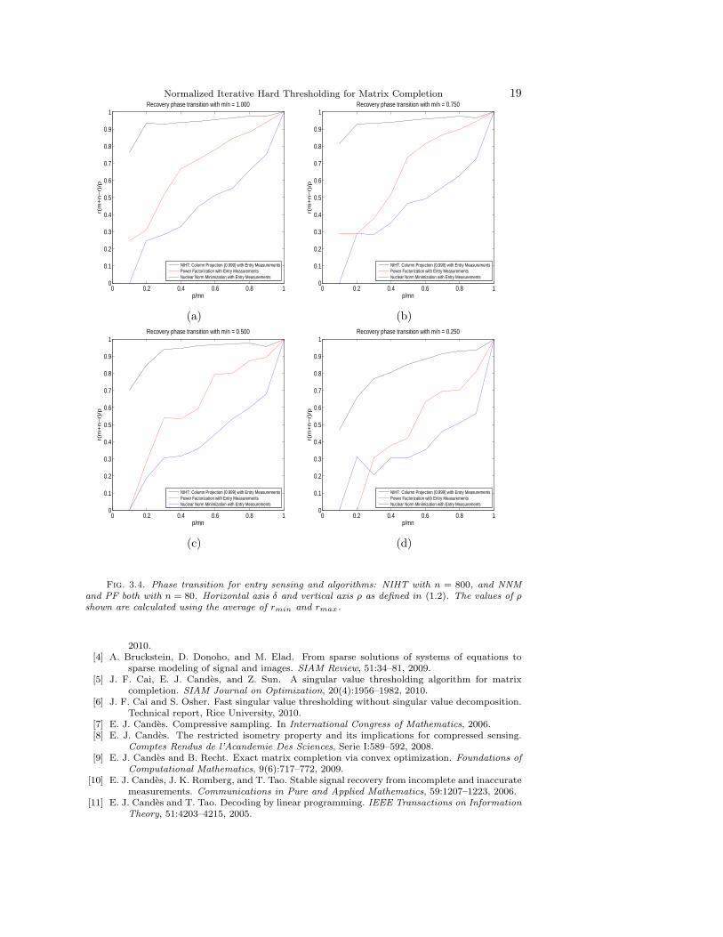
Fig. 3.5. Median time (seconds) for: (a) NIHT with entry sensing, (b) NIHT with Gaussiansensing, (c) IHT with entry sensing, (d) IHT with Gaussian sensing, (e) NNM with entry sensing,(f) NNM with Gaussian sensing, (g) PF with entry sensing, and (h) PF with Gaussian sensing.Entry sensing tests are for m = n = 80 and Gaussian sensing texts for m = n = 40. IHT uses thefixed stepsize µj = 0.65.


0 0.2 0.4 0.6 0.8 10

0.1

0.2

0.3

0.4

0.5

0.6

0.7

0.8

0.9

1

p/(m*n)

r*(m

+n

−r)

/p

0.1

0.15

0.2

0.25

0.3

0.35

0.4

0 0.2 0.4 0.6 0.8 10

0.1

0.2

0.3

0.4

0.5

0.6

0.7

0.8

p/(m*n)

r*(m

+n

−r)

/p

0.2

0.4

0.6

0.8

1

1.2

1.4

(a) (b)

0.2 0.3 0.4 0.5 0.6 0.7 0.8 0.9 10

0.1

0.2

0.3

0.4

0.5

0.6

0.7

0.8

0.9

1

p/(m*n)

r*(m

+n

−r)

/p

0.005

0.01

0.015

0.02

0.025

0.03

0.035

0.2 0.3 0.4 0.5 0.6 0.7 0.8 0.9 10

0.1

0.2

0.3

0.4

0.5

0.6

0.7

0.8

p/(m*n)

r*(m

+n

−r)

/p

0.2

0.4

0.6

0.8

1

1.2

1.4

1.6

1.8

2

2.2

(c) (d)

0.2 0.3 0.4 0.5 0.6 0.7 0.8 0.9 10

0.1

0.2

0.3

0.4

0.5

0.6

0.7

0.8

0.9

1

p/(m*n)

r*(m

+n

−r)

/p

0.1

0.2

0.3

0.4

0.5

0.6

0.7

0.8

0.2 0.3 0.4 0.5 0.6 0.7 0.8 0.9 10

0.1

0.2

0.3

0.4

0.5

0.6

0.7

0.8

p/(m*n)

r*(m

+n

−r)

/p

3.5

4

4.5

5

5.5

6

6.5

(e) (f)

Fig. 3.6. Ratio of median time for NIHT divided by: (a) IHT with entry sensing, (b) IHT withGaussian sensing, (c) NNM with entry sensing, (d) NNM with Gaussian sensing, (e) PF with entrysensing, and (f) PF with Gaussian sensing. Entry sensing tests are for m = n = 80 and Gaussiansensing texts for m = n = 40. IHT uses the fixed stepsize µj = 0.65.


[12] E. J. Candes and T. Tao. The power of convex relaxation: Near-optimal matrix completion.IEEE Transactions on Information Theory, 56(5):2053–1080, 2009.

[13] A. Cohen, W. Dahmen, and R. DeVore. Compressed sensing and best k-term approximation.Journal of the AMS, 22(1):211–231, 2009.

[14] W. Dai and O. Milenkovic. Subspace pursuit for compressive sensing signal reconstruction.IEEE Transactions on Information Theory, 55:2230–2249, 2009.

[15] W. Dai, O. Milenkovic, and E. Kerman. Subspace evolution and transfer (SET) for low-rankmatrix completion. IEEE Transactions on Signal Processing, 59(7):3120–3132, 2011.

[16] D. L. Donoho. Compressed sensing. IEEE Transactions on Information Theory, 52(4):1289–1306, 2006.

[17] D. L. Donoho. Neighborliness polytopes and sparse solution of underdetermined linear equa-tions. Technical report, Stanford University, 2006.

[18] D. L. Donoho and J. Tanner. Precise undersampling theorems. Proceedings of the IEEE,98(6):913–924, 2010.

[19] Y. C. Eldar, D. Needell, and Y. Plan. Unicity conditions for low-rank matrix recovery. Appliedand Computational Harmonic Analysis, 33(2):309–314, 2012.

[20] S. Foucart. Hard thresholding pursuit: an algorithm for compressive sensing. SIAM Journalon Numerical Analysis, 49(6):2543–2563, 2011.

[21] D. Goldfarb and S. Ma. Convergence of fixed-point continuation algorithms for matrix rankminimization. Foundations of Computational Mathematics, 11(2):183–210, 2011.

[22] J. P. Haldar and D. Hernando. Rank-constrained solutions to linear matrix equations usingpower-factorization. IEEE Signal Processing Letters, 16:584–587, 2009.

[23] N. J. A. Harvey, D. R. Karger, and S. Yekhanin. The complexity of matrix completion. SODA2006, Proceedings of the seventeenth annual ACM-SIAM symposium on discrete algo-rithms, pages 1103–1111, 2006.

[24] P. Jain, R. Meka, and I. Dhillon. Guaranteed rank minimization via singular value projection.Proceedings of the Neural Information Processing Systems Conference (NIPS), pages 937–945, 2010.

[25] R. H. Keshavan, A. Montanari, and S. Oh. Matrix completion from a few entries. IEEETransactions on Information Theory, 56(6):2980–2998, 2010.

[26] R. H. Keshavan and S. Oh. Optspace: A gradient descent algorithm on the grassmann manifoldfor matrix completion. http://arxiv.org/abs/0910.5260v2, 2009.

[27] A. Kyrillidis and V. Cevher. Matrix alps: Accelerated low rank and sparse matrix reconstruc-tion. Technical report.

[28] A. Kyrillidis and V. Cevher. Matrix recipes for hard thresholding methods. Technical report.[29] R. M. Larsen. PROPACK (software package). http://sun.stanford.edu/˜rmunk/PROPACK/.[30] K. Lee and Y. Bresler. ADMiRA: Atomic decomposition for minimum rank approximation.

IEEE Transactions on Information Theory, 56(9):4402–4416, 2010.[31] A. S. Lewis and J. Malick. Alternating projections on manifolds. Mathematics of Operations

Research, 33:216–234, 2008.[32] Z. Lin, M. Chen, and Y. Ma. The augmented lagrange multiplier method for exact recovery of

corrupted low-rank matrices. http://arxiv.org/abs/1009.5055, 2010.[33] S. Ma, D. Goldfarb, and L. Chen. Fixed point and bregman iterative methods for matrix rank

minimization. Mathematical Programming Series A, 128(1):321–353, 2011.[34] A. Maleki and D. L. Donoho. Optimally tuned iterative reconstruction algorithms for com-

pressed sensing. IEEE Journal of Selected Topics in Signal Processing, 4(2):330–341,2010.

[35] G. Meyer, S. Bonnabel, and R. Sepulchre. Linear regression under fixed-rank constraints: ariemannian approach. In Proc. of the 28th International Conference on Machine Learning(ICML2011), Bellevue (USA), 2011.

[36] M. Michenkova. Numerical algorithms for low-rank matrix completion problems. Technicalreport, http://www.math.ethz.ch/˜kressner/students/michenkova.pdf, 2011.

[37] D. Needell and J. Tropp. Cosamp: Iterative signal recovery from incomplete and inaccuratesamples. Applied and Computational Harmonic Analysis, 26(3):301–321, 2009.

[38] B. Recht, M. Fazel, and P. A. Parrilo. Guaranteed minimum-rank solutions of linear matrixequations via nuclear norm minimization. SIAM Review, 52(3):471–501, 2010.

[39] B. Recht, W. Xu, and B. Hassibi. Null space conditions and thresholds for rank minimization.Mathematical Programming Series B, pages 175–211, 2011.

[40] U. Shalit, D. Weinshall, and G. Chechik. Online learning in the manifold of low-rank matrices.Neural Information Processing Systems (NIPS spotlight), 2010.

[41] K. Toh and S. Yun. An accelerated proximal gradient algorithm for nuclear norm regularizedleast squares problems. Pacific Journal of Optimization, pages 615–640, 2010.


[42] K. C. Toh, M. J. Todd, and R. H. Tutuncu. SDPT3 4.0(beta) (software package).http://www.math.nus.edu.sg/˜mattohkc/sdpt3.html, July 2006.

[43] B. Vandereycken. Low rank matrix completion by riemannian optimization. submitted, 2012.[44] B. Vandereycken and S. Vandewalle. A riemannian optimization approach for computing low-

rank solutions of lyapunov equations. SIAM Journal on Matrix Analysis and Applications,31(5):2553–2579, 2010.

[45] Z. Wen, W. Yin, and Y. Zhang. Solving a low-rank factorization model for matrix completionby a non-linear successive over-relaxation algorithm. Mathematical Programming Compu-tation, published online, 2012.

normalized iterative hard thresholding for matrix

Documents