survey and recommendations abstract - nasa · metamodels for computer-based engineering design:...
TRANSCRIPT

METAMODELS FOR COMPUTER-BASED ENGINEERING DESIGN:
SURVEY AND RECOMMENDATIONS
Timothy W. Simpson, Jesse Peplinski, Patrick N. Koch, and Janet K. Allen tSystems Realization Laboratory
Woodruff School of Mechanical EngineeringGeorgia Institute of Technology
Atlanta, Georgia 30332-0405, USA
ABSTRACT
The use of statistical techniques to build approximations of expensive computer analysis codes
pervades much of today's engineering design. These statistical approximations, or metamodels,
are used to replace the actual expensive computer analyses, facilitating multidisciplinary,
multiobjective optimization and concept exploration. In this paper we review several of these
techniques including design of experiments, response surface methodology, Taguchi methods,
neural networks, inductive learning, and kriging. We survey their existing application in
engineering design and then address the dangers of applying traditional statistical techniques to
approximate deterministic computer analysis codes. We conclude with recommendations for the
appropriate use of statistical approximation techniques in given situations and how common pitfalls
can be avoided.
1 INTRODUCTION
Much of today's engineering analysis consists of running complex computer codes: supplying
a vector of design variables (inputs) x and computing a vector of responses (outputs) y. Despite
steady advances in computing power, the expense of running many analysis codes remains non-
trivial; single evaluations of aerodynamic or finite-element analyses can take minutes to hours, if
not longer. Moreover, this mode of query-and-response often leads to a trial and error approach to
design whereby a designer may never uncover the functional relationship between x and y and
therefore never identify the "best" settings for input values.
t Corresponding author. Email: [email protected]. Phone/Fax: 404-894-8168/9342.
Draft Version: 12/19/97 Submitted to Research in Engineerhtg Design.
https://ntrs.nasa.gov/search.jsp?R=19990087092 2019-05-29T00:09:19+00:00Z

Statistical techniques are widely used in engineering design to address these concerns. The
basic approach is to construct approximations of the analysis codes that are more efficient to run
and yield insight into the functional relationship between x and y. If the true nature of a computer
analysis code is
y = f(x),
then a "model of the model" or metamodel [62] of the analysis code is
= g(x), and so y = _ +
where E represents both the error of approximation and measurement (random) errors. The most
common metamodeling approach is to apply the design of experiments (DOE) to identify an
efficient set of computer runs (xl, x2, ..., xo) and then use regression analysis to create a
polynomial approximation of the computer analysis code. These approximations then can replace
the existing analysis code while providing:
• a better understanding of the relationship between x and y,
° easier integration of domain dependent computer codes, and
• fast analysis tools for optimization and exploration of the design space by using
approximations in lieu of the computationally expensive analysis codes themselves.
We have found that many applications (including our own) using these methods for computer-
based design are statistically questionable because many analysis codes are deterministic in which
the error of approximation is not due to random effects. This calls into question the subsequent
statistical analyses of model significance. Consequently, we seek to highlight potential statistical
pitthlls in metamodeling and provide general recommendations for the proper use of metamodeling
techniques in computer-based engineering design. In Section 2 we present a review of
metamodeling techniques including regression, neural networks, inductive learning, and kriging.
We conclude Section 2 with an introduction to the general statistical approaches of response
surface methodology and Taguchi's robust design. In Section 3 we describe the engineering
design context for statistical applications, review existing applications and methods and conclude
2

with a closer look at deterministic applications of metamodeling. In Section 4 we present some
recommendations for avoiding pitfalls in using metamodeling, and in Section 5 we conclude by
discussing some more advanced issues that contribute to making metamodeling an active and
interesting research area.
2 REVIEW OF METAMODELING TECHNIQUES
Metamodeling involves (a) choosing an experimental design for generating data, (b) choosing a
model to represent the data, and then (c) fitting the model to the observed data. There are several
options for each of these steps as shown in Figure 1, and we have attempted to highlight a few of
the more prevalent ones. For example, building a neural network involves fitting a network of
neurons by means of backpropagation to data which is typically hand selected while Response
Surface Methodology usually employs central composite designs, second order polynomials and
least squares regression analysis.
EXPERIMENTALDESIGN
(Fractional)Factorial /
Central Composite
Box-Behnken
D-Optimal_
G-Optimal
Orthogonal Array
Plackett-Burman
Hexagon
Hybrid
Latin Hypercube
Select By Hand_
Random Selection
MODELCHOICE
-r Polynomial -(linear, quadratic)
Splines(linear, cubic)
Realization of aStochastic Process
Kernel Smoothing
Radial BasisFunctions
Network ofNeurons
Rulebase or--Decision Tree
MODELFITTING
-_ Least Squares -Regression
WeightedLeast Squares
Regression
Best LinearUnbiased Predictor
Best LinearPredictor
Log-Likelihood
Backpropagation-
"_ Entropy _(info.-theoretic)
SAMPLEAPPROXIMATION
TECHNIQUES
,. Response SurfaceMethodology
Kriging
NeuralNetworks
InductiveLearning
Figure 1. Techniques for Metamodeling
3

In the remainder of this section we provide a brief overview of several of the options listed in
Figure 1. In Section 2.1 the focus is on experimental designs, particularly (fractional) factorial
designs, central composite designs and orthogonal arrays. In Section 2.2 we discuss model choice
and model fitting, focusing on response surfaces, neural networks, inductive learning and kriging.
We conclude with an overview of two of the more common metamodeling techniques, namely,
response surface methodology and Taguchi's robust design.
2.1 Experimental Design
Properly designed experiments are essential for effective computer utilization. In engineering,
traditionally a single parameter is varied (perturbed) and the effects are observed. Alternatively,
combinations of factor settings are assigned either systematically (e.g., grid search) or randomly to
provide an alternative for comparison. Experimental design techniques which were developed for
physical experiments are being applied to the design of computer experiments to increase the
efficiency of these analyses. In this section an overview of different types of experiment designs is
provided along with measures of merit for selecting/comparing different experimental designs.
2.1.1 A Survey of Experimental Desiqns. An experimental design represents a sequence of
experiments to be performed, expressed in terms of factors (design variables) set at specified levels
(predefined values). An experimental design is represented by a matrix X where the rows denote
experiment runs, and the colunms denote particular factor settings.
Factorial Designs: The most basic experimental design is a full factorial design. The number of
design points dictated by a lull factorial design is the product of the number of levels for each
factor. The most common are 2 k (for evaluating main effects and interactions) and 3 k designs (for
evaluating main and quadratic effects and interactions) for k factors at 2 and 3 levels, respectively.
A 23 full factorial design is shown in Figure 2(a).
The size of a full factorial experiment increases exponentially with the number of factors; this
leads to an unmanageable number of experiments. Fractional factorial designs are used when
experiments are costly and many factors are required. A fractional factorial design is a fraction of a
4

full factorial design; the most common are 2 (k-p) designs in which the fraction is 1/2 (p). A half
fraction of the 2 3 full factorial design is shown in Figure 2(b). The reduction of the number of
design points in a fractional factorial design is not without a price. The 2 3 full factorial design
shown in Figure 2(a) allows estimation of all main effects (x 1, x 2, x3), all two factor interactions
(x ix 2, x_x 3 and X2X3) , as well as the three factor interaction (x_ X2X3). For the 23-1 fractional factorial
indicated by the solid dots in Figure 2(b), the main effects are aliased (or biased) with the two
factor interactions. Aliased effects cannot be estimated independently unless they are known (or
assumed) not to exist.
X2 X2
X1 X1
. . ×,,_";,X3
X2
(a) 23Full Factorial (b) 291 Fractional Factorial (c) Composite Design
Figure 2. Basic Three-Factor Designs
Often 2 k and 2 !k-p) designs are used to identify or screen for important factors. When there are
many factors, the 5parsity of effects principle [87] can be invoked whereby the system is assumed
to be dominated by main effects and low order interactions. Thus, two level tractional factorial
designs are used to "screen" factors to identify those with the greatest effects. The sparsity of
effects principle is not always valid, however; Hunter [59] notes that every design provides aliased
estimates: quadratic and cubic effects, if present, bias the estimates of the mean and main effects
when a two level fractional factorial design is used.
One specific family of fractional factorial designs frequently used for screening are two level
Plackett-Burman (PB) designs [103]. These are used to study k=n-1 factors in n=4m design
points. PB designs in which n is a power of two are called geometric designs and are identical to
2 (kp) fractional factorials. If n is strictly a multiple of four, the PB designs are referred to as non-
geometric designs and have very messy alias structures. Their use in practical problems is
5

problematic particularly if the design is saturated (i.e., the number of factors is exactly n-1). If
interactions are negligible, however, these designs allow unbiased estimation of all main effects,
and require only one more design point than the number of factors; they also give the smallest
possible variance [14]. Myers and Montgomery [91] present a more complete discussion of
factorial designs and aliasing of effects. Minimum variance and minimum size designs are
discussed in Section 2.1.2.
Central Composite and Box-Behnken Designs: To estimate quadratic effects, 3 k or 3 (kpl designs
can be used but often require an unmanageable number of design points. The most common
second order designs, configured to reduce the number of design points, are central composite and
Box-Behnken designs.
A central composite design (CCD) is a two level (2 (kp_or 2k) factorial design, augmented by n o
center points and two "star" points positioned at _+_ for each factor. This design, shown for three
factors in Figure 2(c), consists of 2(kP)+2k+no total design points to estimate 2k+k(k-1)/2+l
coefficients. For three factors, setting c_= 1 locates the star points on the centers of the faces of the
cube, giving a face-centered central composite (CCF) design; note that for values of a other than 1,
each factor is evaluated at five levels.
Often it is desirable to use the smallest number of factor levels in an experimental design. One
common class of such designs is the Box-Behnken designs [15]. These are formed by combining
2 k factorials with incomplete block designs. They do not contain points at the vertices of the
hypercube defined by the upper and lower limits for each factor. This is desirable if these extreme
points are expensive or impossible to test. More information about CCD and Box-Behnken
designs can be found in [87].
Orthogonal Arrays: The experiment designs used by Taguchi, orthogonal arrco,s, are usually
simply fractional factorial designs in two or three levels (2 _k-p_and 3 _kp_designs). These arrays are
constructed to reduce the number of design points necessary; two-level L 4, Ltz, and Ll6 arrays, for
example, allow 3, 11, and 15 factors/effects to be evaluated with 4, 12, and 16 design points,
respectively. Often these designs are identical to Plackett-Burman designs [78]. The definition of
6

orthogonality for these arrays and other experiment designs is given in Section 2.1.2. An
overview of Taguchi's approach to parameter design is given in Section 2.3.
"Space Filling" Designs: Many researchers advocate the use of "space filling" designs when
sampling deterministic computer experiments. As discussed by Booker [13], in the "classical"
design and analysis of physical experiments (i.e., using central composite and factorial designs),
random variation is accounted for by spreading the sample points out in the design space and by
taking multiple data points (replicates), see Figure 3. Sacks, et al. [117] state that the "classical"
notions of experimental blocking, replication, and randomization are irrelevant when it comes to
deterministic computer experiments; thus, sample points in DACE should be chosen to fill the
design space. They suggest minimizing the integrated mean squared error (IMSE) over the design
region by using IMSE-optimal designs; the "space filling" design illustrated in Figure 3(b) is an
IMSE optimal design.
10p i 0[0.5 0.5 • • • •
x2 0.0 go _o go x2 0.0 • •
-0.5 -0.5 • • • • •
-1.0 go oo -1.0 • • • •oo
-1.0 -0.5 0.0 0,5 1.0 -I.0 -0.5 0.0 0.5 1.0
xl xl
(a) "Classical" Design (b) "Space Filling" Design
Figure 3. "Classical" and "Space Filling" Designs [adapted from 13]
Koch [63] investigates the use of a modified central composite design which combines half
fractions of a CCI and a CCF to more evenly distribute the points throughout the design space.
Koehler and Owen [66] describe several Bayesian and Frequentist "space filling" designs,
including maximum entropy designs, mean squared-error designs, minimax and maximin designs,
Latin hypercubes, randomized orthogonal arrays, and scrambled nets. Minimax and maxhnin
designs were originally proposed by Johnson, et al. [60] specifically for use with computer
experiments. Sherwy and Wynn [121] and Currin, et al. [35] use the maximum entropy principle
to develop designs for computer experiments. Tang [128] describes orthogonal array-based Latin

hypercubeswhich he assertsare more suitablefor computerexperimentsthan generalLatin
hypercubes.Park [100] discussesoptimal Latin hypercube designs for computer experiments
which either minimize IMSE or maximize entropy, spreading the points out over the design region.
Morris and Mitchell [89] propose maximin distance designs found within the class of Latin
hypercube arrangements since they "offer a compromise between the entropy/maximin criterion,
and good projective properties in each dimension." Owen [99] advocates the use of orthogonal
arrays as suitable designs for computer experiments, numerical integration, and visualization; a
collection of orthogonal array generators is available over the Intemet [98]. A review of Bayesian
experimental designs for linear and nonlinear regression models is given in [24].
2.1.2 Measures of Merit for Evaluating Experimental Designs. Selecting the appropriate
design is essential for effective experimentation: the desire to gain as much information as possible
about the response-factor relationships is balanced against the cost of experimentation. Several
measures of merit are available and useful for evaluating and comparing experimental designs.
Orthogonality, Rotatability, Minimum Variance, and Minimum Bias: To facilitate efficient
estimates of parameters, four desirable characteristics of an experimental design are orthogonality,
rotatability, minimum variance, and minimum bias. A design is orthogonal if, for every pair of
factors x_ and xj, the sum of the cross-products of the N design points
N
E XiuXju
u=-I
For a first order model, the estimates of all coefficients will have minimum variance if theis zero.
design can be configured so that
N
E X2u=N ;u=l
the variance of predictions _ will also have constant variance at a fixed distance from the center of
the design, and the design will also be rotatable.

In second order modeling, Hunter [58] suggests that orthogonality is less important: "If the
objective of the experimenter is to forecast a response at either present or future settings of x, then
an unbiased minimum variance estimate of the forecast _ is required. In the late 1950's Box and
his co-workers demonstrated that rotatability...and the minimization of bias from higher order
terms...were the essential criteria for good forecasting." A design is rotatable if N.Var[_ (x)]/_ z
has the same value at any two locations that are the same distance from the design center. The
requirements for minimum variance and minimum bias designs for second order models are
beyond the scope of this work; we refer the reader to [91] for more information.
Unsaturated�Saturated and Supersaturated Designs: In many cases, the primary concern in the
design of an experiment is its size. Most designs are unsaturated in that they contain at least two
more design points than the number of factors. A saturated design is one in which the number of
design points is equal to one more than the number of factor effects to be estimated. Saturated
fractional factorial designs allow unbiased estimation of all main effects with the smallest possible
variance and size [14]. The most common examples of saturated designs are the Plackett-Burman
two level design and Taguchi's orthogonal arrays. For estimating second order effects, small
composite designs have been developed to reduce the number of required design points. A small
composite design is saturated if the number of design points is 2k+k(k-1)/2+ 1 (the number of
coefficients to be estimated for a full quadratic model). Myers and Montgomery [91 ] note that
recent work has suggested that these designs may not always be good; additional comments on
small composite designs can be found in [16, 77]. Finally, in supersaturated designs the number
of design points is less than or equal to the number of factors [37, 38].
It is most desirable to use unsaturated designs for predictive models, unless running the
necessary experiments is prohibitively expensive. When comparing experiments based on the
number of design points and the information obtained, the D-optimal and D-efficiency statistics are
often used.
D-optimal and D-efficiency: A design is said to be D-optimal if IX' X ]/r?' is maximized where X
is the expanded design matrix which has n rows (one for each design setting) and p columns (one
9

colunm for each coefficient to be estimated plus one colunm for the overall mean). The D-
efficiency statistic for comparing designs, Eq. (1), compares a design against a D-optimal design,
normalized by the size of the matrix in order to compare designs of different sizes.
' / X'X 1/pD-efficiency = (IX Xldesig n ] ]D-optimum) (1)
Other statistics for comparing designs such as G-efficiency, Q-efficiency, and A-optimality have
also been formulated, see, e.g., [91]. We now turn to the issues of model choice and model
fitting.
2.2 Model Choice and Model Fitting
After selecting an appropriate experimental design and performing the necessary computer
runs, the next step is to choose an approximating model and fitting method. Many alternative
models and methods exist, but here we review the four which are most prevalent in the literature:
response surfaces, neural networks, inductive learning, and kriging.
2.2.1 Response Surfaces. Given a response, y,
influencing y, the relationship between y and x is:
and a vector of independent factors x
y = fix) + e , (2)
where e represents random error which is assumed to be normally distributed with mean zero and
standard deviation cr. Since the true response surface function fix) is usually unknown, a response
surface g(x) is created to approximate fix). Predicted values are then obtained using _ = g(x).
The most widely used response surface approximating functions are low-order polynomials.
For low curvature, a first order polynomial can be used as in Eq. (3); for significant curvature, a
second order polynomial which includes all two-factor interactions is available, see Eq. (4).
k
= [30 + Z [3ixi (3)
i=l
k k
= [30 + Z [3iXi + Z [3iiXi 2 + Z Z [3ijXiXj (4)
i=l i=l i j
i<j
10

Theparametersof the polynomials in Eq. (3) andEq. (4) areusually determinedby least
squaresregressionanalysisby fitting theresponsesurfaceapproximationsto existingdata. These
approximationsare normally used tbr prediction within response surface methodology (RSM). A
more complete discussion of response surfaces and least squares fitting is presented in [91]. An
overview of RSM is given in Section 2.3.
2.2.2 Neural Networks. A neural network is composed of neurons (single-unit perceptrons)
which are multiple linear regression models with a nonlinear (typically sigmoidal) transformation
on y. If the inputs to each neuron are denoted {xl, x2, ..., x a }, and the regression coefficients are
denoted by the weights, w_, then the output, y, might be given by
1y-1 + enrr (5)
where 11= Y_w_xi + 13(where 13is the "bias value" of a neuron), and T is the slope parameter of the
sigmoid defined by the user. A neural network is then created by assembling the neurons into an
architecture; the most common of which is the multi-layer feedforward architecture, see Figure 4.
Iv Input Hidden OutputInputs ' Units Layer UnitsI
I xl _ 1]=_WiX i+_/ X2--W l I
ut ' _I
!
li 'wn _ Y_ I!
It I
I
!
!
(a) Single-Unit Perceptron (b) Feedforward Two-layer Architecture
Figure 4. Typical Neuron and Architecture
There are two main issues in building a neural network: (1) specifying the architecture and (2)
training the neural network to pertbrm well with reference to a training set. "To a statistician, this
is equivalent to (i) specifying a regression model, and (ii) estimating the parameters of the model
11

given a set of data" [30]. If the architecture is made large enough, a neural network can be a nearly
universal approximator [115]. Hajela and Berke [54] review the use of neural networks in
structural analysis and design.
"Training" a neural network is the determination of the proper values for all weights, w i, in the
architecture and is usually done by backpropagation [115]; this requires a set of n training data
points [(xl,y_), (x2,y2) .... , (xp,yp)}. For a network with output y, the performance is
E =_ (yp- _p)2 (6)P
where _ p is the output that results from the network given input xp, and E is the total error of the
system. The weights are then adjusted in proportion to
0E 0y (7)Oy Ow_j"
Neural networks are best suited for approximating deterministic functions in regression-type
applications. "In most applications of neural networks that generate regression-like output, there is
no explicit mention of randomness. Instead, the aim is function approximation" [30]. Typical
applications of neural nets are speech recognition and handwritten character recognition where the
data is complex and of high dimensionality. Networks with tens of thousands of paranaeters have
been used but the requisite gathering of training data and calculation of model paranaeters can be
extremely computationally expensive. Cheng and Titterington [30] comment that "...the procedure
is to toss the data directly into the NN software, use tens of thousands of parameters in the fit, let
the workstation run 2-3 weeks grinding away doing the gradient descent, and voild, out comes the
result." Rogers and LaMarsh [ 111 ] describe parallel computing eftbrts aimed at reducing the time
required to "train" neural networks.
2.2.3 In d u eti ve I.e a r n in .q. Inductive learning is one of five main paradigms of machine learning
that also include neural networks, case-based learning, genetic algorithms, and analytic learning
[68]. Of these five, inductive learning is the most akin to regression and metamodeling and is
therefore the focus here. An inductive learning system induces rules from examples; the
12

fundamental modeling constructs are condition-action rules which partition the data into discrete
categories and can be combined into decision trees for ease of interpretation, see Figure 5.
y = f(xl,x2) ]====================================================================
Y = Yl Y = Y2 Y = Y3 Y = Y4
Figure 5. A Decision Tree
Training data are required in the form {(xl,yl),(x2,y2) .... , (xn,yn) } where x i is a vector of
attribute values (e.g., processing parameters and environmental conditions), and each Yi is a
corresponding observed output value. Although attributes and outputs can be real-valued, the
method is better suited to discrete-valued data; real values must often be transformed into discrete
representations [41]. Once the data has been collected, training algorittuns build a decision tree by
selecting the "best" divisive attribute and then recursively calling the resulting data subsets.
Although trees can be built by selecting attributes randomly, it is more efficient to select attributes
that minimize the amount of information needed tbr category membership. The mathematics of
such an information-theoretic approach are given in [41].
Many of the applications of inductive learning have been in process control and diagnostic
systems, and inductive learning approaches can be used to automate the knowledge-acquisition
process of building expert systems. Furthermore, although decision trees appear best suited for
applications with discrete input and output values, there are also applications with continuous
variables that have met with greater success than standard statistical analysis. Leech [71] reports a
process-control application where "Standard statistical analysis methods were employed with
13

limited success.Someof thedatawerenon-numerical,thedependenciesbetweenvariableswere
notwell understood,andit wasnecessaryto simultaneouslycontrol severalcharacteristicsof the
final productwhile workingwithin systemconstraints.Theresultsof thestatisticalanalysis,a set
of correlationsfor eachoutputof interest,weredifficult for peopleresponsiblefor theday-to-day
operationto interpretanduse." Additionalexamplescanbe foundin [41,68].
2.2.4 Kriging. Since many computer analysis codes are deterministic and therefore not subject to
measurement error, the usual measures of uncertainty derived from least-squares residuals have no
obvious meaning (cf., [117]). Consequently, some statisticians (see, e.g., [13, 66, 117, 138])
have suggested modeling responses as a combination of a polynomial model plus departures of the
form:
y(x) = f(x) + Z(x) (8)
where y(x) is the unknown function of interest, f(x) is a known polynomial function of x, and
Z(x) is the realization of a nomaally distributed Gaussian random process with mean zero, variance
2, and non-zero covariance. The f(x) term in Eq. (8) is similar to the polynomial model in a
response surface and provides a "global" model of the design space; in many cases f(x) is simply
taken to be a constant term, see, e.g., [117, 139].
While f(x) "globally" approximates the design space, Z(x) creates "localized" deviations so
that the kriging model interpolates the n S sampled data points. The covariance matrix of Z(x) is
given by:
Cov[Z(xi),Z(xJ)] = cr2 R([R(xi, x j)]. (9)
where R is the correlation matrix, and R(xi,x j) is the correlation function between any two of the n s
sampled data points x _ and x j. R is a (ns x ns) symmetric matrix with ones along the diagonal. The
correlation function R(x_,x j) is specified by the user; Sacks, et al. [117] and Koehler and Owen
[66] discuss several correlation functions which may be used. In our work, we have employed a
Gaussian correlation function of the form:
14

i j) -_ iR(x,x =exp[-Ek=,0dxk-x{l'l (10)
where ok are the unknown correlation parameters used to fit the model, and the xki and xkj are the
k 'h components of sample points x i and x j. In some cases using a single correlation parameter
gives sufficiently good results, see, e.g., [94, 117].
Predicted estimates, _ (x), of the response y(x) at untried values of x are given by:
= _ + rT(x)R -' (y-f_) (1 1)
where y is the colunm vector of length n, which contains the values of the response at each sample
point, and f is a column vector of length n, which is filled with ones when f(x) is taken as a
constant. In Eq. (11), rT(x) is the correlation vector of length n s between an untried x and the
sampled data points {x 1, x 2, ..., x n' } and is given by:
FT(x) = [R(x,xl), R(x,x 2) ..... R(x,xnS)] T (12)
In Eq. (11), _ is estimated using Eq. (13).
= (fTR-lf)-I fTR-ly. (13)
The estimate of the variance, _2, from the underlying global model (not the variance in the
observed data) is given by
_2 = (Y- f_)TR-t(Y - 1_) (14)
U s
where f(x) is assumed to be the constant _. The maximum likelihood estimates (i.e., "best
guesses") for the Ok in Eq. (10) used to fit the model are found by maximizing [13]:
[n ln(d 2) + lnlRl] (15)2
15

for 0k> 0 where both _2 and ]R] are both functions of % While any values for the 0k create an
interpolative approximation model, the "best" kriging model is found by solving the k-dimensional
unconstrained nonlinear optimization problem given by Eq. (15).
Depending on the choice of correlation function in Eq. (10), kriging can either "honor the
data," providing an exact interpolation of the data, or "smooth the data," providing an inexact
interpolation [34]. Finally, it should be noted that kriging is different from fitting splines (i.e.,
non-parametric regression models). In several comparative studies kriging performs as well as, if
not better than, splines [69].
2.2.4 Additional Metamodelinq Approaches. For the reader's convenience, we include
references for some alternative metamodeling techniques which have not been discussed in the
previous subsections. Rasmussen [106] offers an accumulated approximation technique for
structural optimization which refines the approximation of objective and constraint functions by
accumulating the function values of previously visited points. Similarly, Bailing and Clark [4]
describe weighted and gradient-based approximations for use with optimization which utilize
weighted sums of exact function values at sample points. Friedman [45] describes multivariate
adaptive regression splines (MARS): a flexible regression modeling method based on recursive
partitioning and spline fitting for high dimensional data. Dyn, et al. [39] use radial basis functions
to build global approximation surfaces to interpolate smooth data. Wang, et al. [137] present
multivariate Hemrite approximations for multidisciplinary design optimization which uses data
generated during the course of iterative optimization; it is compared against linear, reciprocal, and
other standard approximations but shows inefficiencies because it requires more data points.
Finally, Friedman and Steutzle [46] introduce projection pursuit regression which works well in
high-dimensional (< 50) data and with large data sets (can handle 200,000+ data points); project
pursuit regression takes the data and generates different projections of it along linear combinations
of the variables; an optimizer finds the best projections and builds a predictor by summing them
together with arbitrary levels of precision.
16

This concludes our discussion on experimental design, model selection and model fitting. We
now turn to more general methods for experimental design and modeling building.
2.3 Experimentation and Metamodeling Strategies
Two widely used methods incorporating experimental design, model building, and prediction
are response surface methodology and Taguchi's robust design or parameter design. A brief
overview of these two approaches is provided.
2.3.1 Response Surface Methodology (RSM). Different authors describe RSM differently.
Myers, et al. [90] define RSM as "a collection of tools in design or data analysis that enhance the
exploration of a region of design variables in one or more responses." Box and Draper [16] state
that, "Response surface methodology comprises a group of statistical techniques for empirical
model building and model exploitation. By careful design and analysis of experiments, it seeks to
relate a response, or output variable, to the levels of a number of predictors, or input variables, that
affect it." Finally, Myers and Montgomery [91 ] state that RSM "is a collection of statistical and
mathematical techniques useful for developing, improving, and optimizing process. It also has
important applications in the design, development, and formulation of new products, as well as in
the improvement of existing product designs."
The "collection of statistical and mathematical techniques" of which these authors speak refers
to the design of experiments (Section 2.1), least squares regression analysis and response surface
model building (Section 2.2.1), and "model exploitation," exploring a factor space seeking
optimum factor settings. The general RSM approach includes all or some of the following steps:
i) screening: when the number of factors is large or when experimentation is expensive,
screening experiments are used to reduce the set of factors to those that are most influential to
the response(s) being investigated;
ii) .first order experimentation: when the starting point is far from the optimum point or when
knowledge about the space being investigated is sought, first order models and an approach
17

such as steepest ascent are used to "rapidly and economically move to the vicinity of the
optimum" [88];
iii) second order experimentation: after the best solution using first order methods is obtained, a
second order model is fit in the region of the first order solution to evaluate curvature effects
and to attempt to improve the solution.
A more detailed description of RSM techniques and tools can be found in [91], and a
comprehensive review of RSM developments and applications from 1966-1988 is given in [90].
In Section 3 we review recent applications in aerospace and mechanical engineering design, but
first we discuss Taguchi's robust design approach.
2.3.2 Taquchi's Robust Desiqn. Genichi Taguchi developed an approach for industrial
product design built on statistically designed experiments. Taguchi's robust design for quality
engineering includes three steps: system design, parameter design, and tolerance design [ 18]. The
key step is parameter design within which statistical experimentation is incorporated.
Rather than simply improving or optimizing a response value, the focus in parameter design is
to identify factor settings that minimize variation in performance and adjust the mean performance
to a desired target in order to minimize the associated loss. Factors included in experimentation
include control factors and noise factors; control factors are set and held at specific values, while
noise factors cannot be controlled, e.g., shop floor temperature. The evaluation of mean
performance and performance variation is accomplished by "crossing" two orthogonal anays
(Section 2.1.1). Control factors are varied according to an inner array, or "control", array, and for
each run of the control array, noise factors are varied according to an outer, or "noise", array. For
each control factor experiment, a response value is obtained for each noise factor design point.
The mean and variance of the response (measured across the noise design points) are calculated.
The performance characteristic used by Taguchi is a signal-to-noise (S/N) ratio defined in terms of
the mean and vm-iance of the response. Several alternate S/N ratios are available based on whether
lower, higher, or nominal response values are desired, see, e.g., [ 112].
18

TheTaguchiapproachdoesnot explicitlyincludemodelbuildingandoptimization.Analysisof
experimentalresultsis usedto identify factoreffects, to plan additionalexperiments,andto set
factorvaluesfor improvedperformance.A comprehensivediscussionof theTaguchiapproachis
givenin [102, 112]. Taguchimethodshavebeenusedextensivelyin engineeringdesignandare
oftenincorporatedwithin traditionalRSMfor efficient,effective,and robust design [91 ]. These
applications and their implications for engineering design are discussed next.
3 METAMODELING IN ENGINEERING DESIGN
How are the metamodeling techniques of the previous section employed in engineering design ?
All of these techniques can be used to create approximations of existing computer analyses, and
produce fast analysis modules for more efficient computation. These metamodeling techniques
also yield insight into the functional relationship between input and output parameters.
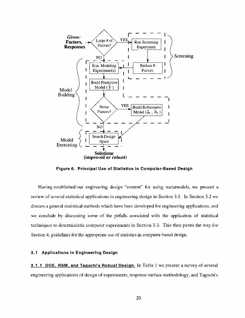
Where would such models be useful? A designer's goal is usually to arrive at improved or
robust solutions which are the values of design variables that best meet the design objectives as
shown in Figure 6. A search for these solutions usually relies on an optimization technique which
generates and evaluates many potential solutions in the path toward design improvement; thus, fast
analysis modules are an imperative.
When are metamodels usefitl or appropriate? In the later stages of design when detailed
information about specific solutions is available, highly accurate analysis is essential. In the early
stages of design, however, the focus is on generating, evaluating, and comparing potential
conceptual configurations. The early stages of design are characterized by a large amount of
information, often uncertain, which must be managed. To ensure the identification of a "good"
system configuration, a comprehensive search is necessary. In this case, the tradeoff between
accuracy and efficiency may be appropriate. The creation of metamodels allows fast analysis,
facilitating both comprehensive and efficient design space search at the expense of a (hopefully
slight) loss of accuracy.
19
Given:
Factors,Responses
IModel /
Building 1
Model
Exercising
Run ScreeningExperiment
[d Run Modeling _ Reduce#I Experiment(s) Factors
Build Predictive I I
Model(_) I I
_ Build Robustness
__ ! Model (_y, "_y)
Solutions(improved or robust)
il,I
I1,I
I
I
I
_1
> Screening
Figure 6. Principal Use of Statistics in Computer-Based Design
Having established our engineering design "context" /'or using metamodels, we present a
review of several statistical applications in engineering design in Section 3.1. In Section 3.2 we
discuss a general statistical methods which have been developed for engineering applications, and
we conclude by discussing some of the pitfalls associated with the application of statistical
techniques to deterministic computer experiments in Section 3.3. This then paves the way tbr
Section 4, guidelines t'or the appropriate use of statistics in computer-based design.
3.1 Applications in Engineering Design
3.1.1 DOE, RSM, and Taguchi's Robust Design. In Table 1 we present a survey of several
engineering applications of design of experiments, response surface methodology, and Taguchi's
2O

robustdesignapproach.Most of theseexamplescomefrom aerospaceandmechanicalengineering
designapplicationspresentedatconferencesin recentyears.A reviewof approximationconcepts
usedin structuraldesigncanbefoundin [7].
Someobservationsregardingour findingsareasfollows.
• Central composite designs and D-optimal designs seem to be preferred among aerospace
engineers while orthogonal arrays (OAs) are preferred by mechanical engineers; grid and random
point searches are seldom used since they are less efficient.
• Optimization seems to be the principal driver for aerospace applications of DOE and RSM; these
types of applications typically involve the use of computer intensive analysis and optimization
routines, and DOE and RSM is a logical choice for increased efficiency.
• Mechanical engineers usually use OAs and Taguchi's approach for robust design and the signal-
to-noise ratio for parameter and tolerance design.
• Very few designers actually model Taguchi's loss function directly (see, e.g., [9]); many prefer
to model the response instead.
• Most applications use second order response surface models; there are only a few cases where
higher order (see, e.g., [136]) and mixed polynomial models (see, e.g., [113]) are used for
engineering design.
• When orthogonal arrays are used, special care must be taken to avoid aliasing main effects with
interactions, unless the interactions are known (or assumed) to be insignificant.
• Most applications utilize least squares regression analysis when fitting a model; only a few use
stepwise regression, and this is usually because the model is not second order.
21

Table 1. Survey of Engineering Applications of DOE, RSM, andTaguchi's RobustDesign
Experimental Response Tetguchi
Design Surface Method Medhod
FilU_ng:
Balsbanov. et al. [3] x x 2nd X X
Bauer and Kr elbs[8] x x x 2rid x x S/N
Beard and Su_efland 19] X x X L
Chert, et al [25} x x L>nd x R
Chi a_l Bloebaum [31] x x R
Engebnd, el al, [40] x X 2_d x
GadaJlsh and EIM a/aghy [47] X x 2rid x x x
131iuntaket al. {51 ] x X 2rid x
Giunta, et al. [_>3] x X X X 2rid x
Healy, et aL [_] X X 2rid x X
Hong, et _. (56} X X I 2rid x x SiN
Koch et al. [64] x x 2rid x
Korng(_d a_l Gab¢iele [67] x 2rid x
Li, et al. [74] x 2rid X X S/N
M,swts etal. [81] x x 2rid x R
Mavris el aL [83] X X 2rid X R
Rotrx et aJ.(113] x x Mix X
Rowel, et BJ. [114J x x x 21_1 x x x
Stanley, et al. J126] x X x R
Sund_, el _d. [ 127] x x x a
Unal el a1.[130] X x 2nd x
Unal. el al. l13t] x x x R
Unal, el al [132] x x x x 2nd X R
Unal. el al, [ 133] x x 2nd X
Venire, el 81.[ 136] x x 4_ X
YLI and Istfil [ 146] X x 2nd x x R
3.1.1 Kri.qing Applications. Kriging, also referred to as DACE (Design and Analysis of
Computer Experiments after the inaugural paper [117]) modeling, has found limited use in
engineering design applications perhaps because of the lack of readily available software to fit
kriging models, the added complexity of fitting a kriging model, or the additional effort required to
use a kriging model. Simpson, et al. [124] detail a preliminary comparison of second order
response surface models and kriging models for the multidisciplinary design of an aerospike nozzle
which has three geometry (design) variables; neither the kriging models nor the response surface
models consistently outperform the other in this engineering example. Giunta [50] presents an
investigation into the use of kriging for the multidisciplinary design optimization of a High Speed
Civil Transport aircraft. He explores a five and a ten variable design problem, observing that the
kriging and response surface modeling approaches yield similar results due to the quadratic trend
of the responses. Osio and Amon [94] have developed an extension of DACE modeling for
22

numerical optimization which uses a multistage strategy for refining the accuracy of the model; they
have applied their approach to the thermal design of an embedded electronic package which has 5
design variables. Booker, et al. [12] solve a 31 variable helicopter rotor structural design problem
using an similar approximation methodology based on kriging. Booker [11] extend the helicopter
rotor design problem to include 56 structural variables to examine the aeroelastic and dynamic
response of the rotor. Welch, et al. [138] describe a kriging-based approximation methodology
which they use to identify important variables, detect curvature and interactions, and produce a
useful approximation model for two 20 variable problems using only 30-50 runs of the computer
code; they claim their method can cope with up to 30-40 variables provided factor sparsity can be
exploited. Trosset and Torczon [ 129] have developed a numerical optimization strategy which
incorporates DACE modeling and pattern search methods for global optimization. Cox and John
[32] have developed the Sequential Design for Optimization method which uses lower confidence
bounds on predicted values of the response for the sequential selection of evaluation points during
optimization. Both approaches have shown improvements over traditional optimization approaches
when applied to a variety of standard mathematical test problems.
3.2 Existing Methods and Tools in Engineering Design
In this section we present some methods and tools developed specifically for engineering
which incorporate statistical techniques from Section 2. Since the Taguchi approach and RSM
have been widely applied in engineering design, a literature review comparing these approaches is
given first. This is followed by an overview of some methods and "tools" that have been
developed for general design applications. These include the Robust Concept Exploration Method,
the Variable-Complexity Response Surface Modeling Method, and Concurrent SubSpace
Optimization to name a few.
3.2.1 Taguchi Approach vs. RSM. The Taguchi approach and RSM have been applied
extensively in engineering design. It is commonly accepted that the principles associated with the
Taguchi approach are both useful and very appropriate for industrial product design. Ramberg, et
23

al. [105] suggestthat"the lossfunctionandtheassociatedrobustdesignphilosophyprovidefresh
insightinto theprocessof optimizingor improvingthesimulation'sperformance."Two aspectsof
theTaguchiapproachareoftencriticized: thechoiceof experimentaldesign(orthogonalarrays,
innerandouter)andthelossfunction(signal-to-noiseratio). It hasbeenarguedanddemonstrated
thattheuseof a singleexperimentcombiningcontrolandnoisefactorsismoreefficient [122,131,
139].Thedrawbacksof combiningresponsemeanandvarianceinto asinglelossfunction (signal-
to-noiseratio)arewell-documented.Manyauthorsadvocatemeasuringtheresponsedirectly and
separatelytrackingmeanandvariance(cf., [27, 105,139]). However,Shoemaker,et al. [122]
warnthat a"potentialdrawbackof theresponse-modelapproachis thatit dependsmorecritically
thantheloss-modelapproachonhow well themodelfits."
Given the wide acceptanceof Taguchirobust designprinciplesand the criticisms, many
advocateacombinedTaguchi-RSMapproachor simply usingtraditionalRSMtechniqueswithin
theTaguchiframework[78, 90,91,105]. Webelievethatorthogonalinnerandouterarrays,and
singlecompositeexperimentseachhaveadvantagesanddisadvantagesandappropriateuses,and
that separateobservationof meanand varianceleadsto useful insight. Regardless,the core
principlesof bothTaguchiandRSMprovideafoundationfor manyof thespecificdesignmethods
discussedin Section3.2.2.
3.2.2 An Overview of Existinq Methods. The Robust Concept Exploration Method (RCEM)
facilitates quick evaluation of different design alternatives and generation of top-level design
specifications in the early stages of design [25, 26]. Foundational to the RCEM is the integration
of robust design principles, DOE, RSM, and the compromise Decision Support Problem (a
multiobjective decision model). The RCEM has been applied to the multiobjective design of a
High Speed Civil Transport [25, 65], a family of General Aviation Aircraft [123], a turbine lift
engine [64], a solar-powered irrigation system 128], and a flywheel [70]; to manufacturing
simulation [101 ]; and to maintainability design of aircraft engines [93]. A preliminary investigation
into the use of DOE and neural networks to augment the capabilities of response surface modeling
within the RCEM is given in [29].
24

The Variable-Complexity Response Surface Modeling (VCRSM) Method uses analyses of
varying fidelity to reduce the design space to the region of interest and build response surface
models of increasing accuracy (see, e.g., [51, 52]). The VCRSM method employs DOE and RS
modeling techniques and has been successfully applied to the multidisciplinary wing design of a
high speed civil transport (see, e.g., [2, 3, 51, 53, 61]), to the analysis and design of composite
curved channel frames [80], to the structural design of bar trusses [113], to predict the fatigue life
of structures [135], to reduce numerical noise inherent in structural analyses [53, 136] and shape
design problems using fluid flow analysis [92], and to facilitate the integration of local and global
analyses for structural optimization [48, 104, 134]. Coarse-grained parallelization of analysis
codes for efficient response surface generation has also been investigated [ 17, 61].
Concurrent SubSpace Optimization (CSSO) uses data generated during concurrent subspace
optimizations to develop response surface approximations of the design space. Optimization of
these response surfaces forms the basis for the subspace coordination procedure. The data
generated by the subspace optimizers is not unifomaly centered about the current design as in CCD
or other sampling strategies, but instead follows the descent path of the subspace optimizers. In
[109, 108, 110], interpolating polynomial response surfaces are constructed which have either a
first or second order basis for use in the CSSO coordination procedure. In [140, 141], a modified
decomposition strategy is used to develop quadratic response surfaces tbr use in the CSSO
coordination procedure. Finally, in [118-120] artificial neural network response surfaces are
developed for use in the CSSO coordination procedure.
Robust Design Simulation (RDS) is a stochastic approach which employs the principles of
Integrated Product and Process Development (IPPD) for the purpose of determining the optimum
values of design factors and proposed technologies (in the presence of uncertainty) which yield
affordable designs with low variability. Toward this end, RDS combines design of experiments
and response surface metamodels with Monte Carlo simulation and Fast Probability Techniques
(see, e.g., [6]) to achieve customer satisfaction through robust systems design [83]. RDS has
been applied to the design of a High Speed Civil Transport aircraft [81, 83] and very large
25

transports [82]. RDS has also been used to study the economic uncertainty of the HSCT [36, 84]
and the feasibility/viability of aircraft [85].
NORMAN/DEBORA is a TCAD (Technology Computer Aided Design) system incorporating
advanced sequential DOE and RSM techniques to aid in engineering optimization and robust design
[22]. NORMAN/DEBORA includes a novel design of experiments concept--Target Oriented
Design--a unique parameter transformation technique--RATIOFIND--and a non-linear,
constrained optimizer--DEBORA [23]. It has been successfully employed for semiconductor
integrated circuit design and optimization [20, 21, 23, 57]. An updated and more powerful version
of NORMAN/DEBORA is being offered as LMS Optimus [75].
The Probabilistic Design System (PDS) being developed at Pratt and Whitney uses Box-
Behnken designs and response surface methodology to perform probabilistic design analysis of
gas turbine rotors [43, 42]. Fox [44] describes twelve criteria which are used to validate the
response surfaces which are used in combination with cheap-to-run analyses in a Monte Carlo
Simulator to estimate the corresponding distributions of the responses and minimum life of system
components. Adamson [1] describes issues involved with developing, calibrating, using, and
testing the PDS and discusses Pratt and Whitney's plans to validate the PDS by designing,
building, and testing actual parts.
DOE/Opt is a prototype computer system for DOE, RSM, and optimization [10]. It has been
used in semiconductor process/device design including process/device optimization, simulator
tuning, process control recipe generation, and design/'or manufacturability.
Hierarchical and Interactive Decision Refinement (HIDER) is a methodology for concept
exploration in the early stages of design. It integrates sinmlation, optimization, statistical
techniques, and machine learning to support design decision making [107, 142]. The
methodology is used to hierarchically refine/reduce "a large initial design space through a series of
multiple-objective optimizations, until a fully specified design is obtained" [142]. HIDER uses the
Adaptive Interactive Modeling System (AIMS) [76] to decompose the design space using distance-
26

based, population-based, and hyperplane-based 'algorithms. HIDER and AIMS have been applied
to the design of a cutting process [76], a diesel engine [142, 143], and a wheel loader [107].
Other approaches incorporating statistical techniques in engineering design exist; only a few
have been included here. Our focus is not on the methods, but on the appropriateness of the
statistical techniques; many of the examples to which these methods have been applied employ
deterministic computer experiments in which the application of statistical techniques is
questionable. Associated issues are discussed in the next section.
3.3 A Closer Look at Experimental Design for Deterministic Computer Experiments
Since engineering design usually involves exercising deterministic computer analysis codes,
the use of statistical techniques for creating metamodels warrants a closer look. Given a response
of interest, y, and a vector of independent factors x thought to influence y, the relationship
between y and x (see Eq. (2)) includes the random error term e. To apply least squares regression,
error values at each data point are assumed to have identical and independent normal distributions
with means of zero and standard deviations of _, or E_i.i.d. N(0,_2), see Figure 7(a). The least
squares estimator then minimizes the sum of the squared differences between actual data points and
predicted values. This is acceptable when no data point actually lies on the predicted model
because it is assumed that the model "smoothes out" random error. Of course, it is likely that the
regression model itself is merely an approximation of the true behavior of x and y so that the final
relationship is
y = g(x) + Ebi_ + Ereaado m (16)
where Ebi,_represents the error of approximation. However, tbr deterministic computer analyses as
shown in Figure 7(b), er_dom has mean zero and variance zero, yielding the relationship
y = g(x) + Ebi_ . (17)
27

Y Y
- N(O,
i!il// X -_= g(x): second o(,_least squares f,ider
(a) Non-Deterministic Case
Figure 7.
.............................°I
t " y = g(x) = spline fit
(b) Deterministic Case
Deterministic and Non-Deterministic Curve Fitting
hv
X
The deterministic case in Eq. (17) conflicts sharply with the methods of least squares
regression. Unless ebi_ is i.i.d. N(0,_ 2) the assumptions for statistical inference from least squares
regression are violated. Further, since there is no random error it is not justifiable to smooth
across data points; instead the model should hit each point exactly and interpolate between them as
in Figure 5(b). Finally, most standard tests for model and parameter significance are based on
computations of Er._omand therefore cannot be computed. These observations are supported by
literature in the statistics community; as Sacks, et al. [117] carefully point out that because
deterministic computer experiments lack random error:
• response surface model adequacy is determined solely by systematic bias,
• the usual measures of uncertainty derived from least-squares residuals have no obvious
statistical meaning (deterministic measures of uncertainty exist, e.g., max. lY (x) - y(x)[ over
x, but they may be very difficult to compute), and
• the classical notions of experimental blocking, replication and randomization are irrelevant.
28

Furthermore, some of the methods for the design and analysis of physical experiments (see,
e.g., [14, 16, 91] are not ideal for complex, deterministic computer models. "In the presence of
systematic error rather than random error, statistical testing is inappropriate" [139]. A discussion
of how the model should interpolate the observations can be found in [116].
So where can these methods go wrong? Unfortunately it is easy to misclassify the Ebi_ term
from a deterministic model as Erandomand then proceed with standard statistical testing. Several
authors have reported statistical measures (e.g., F-statistics and root mean square error) to verify
model adequacy, see, e.g., [55, 64, 132, 136, 139]. However, these measures have no statistical
meaning since they assume the observations include a random error term with a mean of zero and a
non-zero standard deviation. Consequently, the use of stepwise regression for polynomial model
fitting is also inappropriate since it utilizes F-statistics when adding/removing model parameters.
Some researchers (see, e.g., [51, 53, 92, 135, 136]) have used metamodeling techniques for
deterministic computer experiments containing numerical noise. Metamodels are used to smooth
the numerical noise which inhibits the performance of gradient based optimizers (cf., [53, 4]).
When constructing the metamodels, the numerical noise is used as a surrogate for random error,
and the standard least-squares approach is then used to determine model significance. The idea of
equating numerical noise to random error warrants further investigation into the sources and nature
of this "deterministic" noise.
How can model accuracy be tested? R-Squared (the model sum of squares divided by the total
sum of squares) and R-Squared_adjusted (which takes into account the number of parameters in
the model) are the only measures for verifying model adequacy in detenninistic computer
experiments. This measure is often insufficient; a high R-Squared value can be deceiving.
Residual plots may be helpful tbr verifying model adequacy, identifying trends in data, examining
outliers, etc; however, validating the model using additional (different) data points is essential.
Maximum absolute error, average absolute error, and root mean square error for the additional
validation points can be calculated to assess model accuracy, see, e.g., [124, 136]. Otto, et al.
[95, 96] and Yesilyurt and Patera [145] have developed a Bayesian-validated surrogate approach
29

which uses additionalvalidationpoints to makequalitativeassessmentsof the quality of the
approximationmodelandprovidetheoreticalboundson thelargestdiscrepancybetweenthemodel
and theactualcomputeranalysis. They have applied their approach to optimization of multi-
element airfoils [96], design of trapezoidal ducts and axisymmetric bodies [97], and optimization
of an eddy-promoter heat exchanger [144, 145]. Finally, an alternative method which does not
require additional points is leave-one-out cross validation [86]. Each sample point used to fit the
model is removed one at a time, the model is rebuilt without a sample point, and the difference
between the model without the sample point and actual value at the sample point is computed for all
of the sample points.
Given the potential problems in applying least-squares regression to deterministic applications,
the trade-off then is between appropriateness and practicality. If a response surface is created to
model data from a deterministic computer analysis code using experimental design and least
squares fitting, and if it provides good agreement between predicted and actual values, then there is
no reason to discard it. It should be used, albeit with caution. However, it is important to
understand the fundamental assumptions of the statistical techniques employed to avoid misleading
statements about model significance. In the next section we offer some guidelines for the
appropriate use of statistical metamodeling with deterministic computer analyses.
4 GUIDELINES AND RECOMMENDATIONS
How can a designer apply metamodeling tools while avoiding the pitfalls described in Section
3.3? This can either be answered from the bottom up (tools -> applications, Section 4.1) or from
the top down (motives -> tools, Section 4.2).
4.1 Evaluation of Metamodeling Techniques
There are two components to this section. The first is an evaluation of the four metamodeling
techniques described in Section 2.2. The second component is choosing an experimental design
which has more direct applicability to response surface methods. Determining what experimental
3O

designsaremost appropriatefor theothermetamodelingtechniquesdiscussedin Section2.2are
openresearchareas.
4.1.1 Evaluation of Model Choice and Model Fittinq Alternatives. Some guidelines for the
evaluation of the metamodeling techniques presented in Section 2.2 are summarized in Table 2.
Table 2. Recommendations for Model Choice and Use
Model Choice
Responses Surfaces
Neural Networks
Rule Induction /Inductive Learning
Kriging
Characteristics/Appropriate Uses• well-established and easy to use• best suited for applications with random error
• appropriate for applications with < 10 factors• good for highly nonlinear or very large problems
(- 10,000 parameters)• best suited for deterministic applications• high computational expense (often > 10,000
training data points); best for repeated application• best when factors and responses are discrete-
valued
• form of model is rules or decision tree; better suited
to dia_nosis than engineerin_ design• extremely flexible but complex• well-suited for deterministic applications• can handle applications with < 50 factors• limited support is currently available tbr
implementation
Response Surfaces: primaIily intended for applications with random error; however, they have
been used successfully in many engineering design applications. It is the most well-established
metamodeling technique and is probably the easiest to use, provided the user is aware of the
possible pitfalls described in Section 3.3.
Neural Networks: nonlinear regression approach best suited to deterministic applications which
require repeated use. Building a neural network for a one-shot use can be extremely inefficient due
to the computational overhead required.
Inductive Learning: modeling technique most appropriate when input and output factors are
primarily discrete-valued or can be grouped. The predictive model, in the fore1 of condition-action
mrs or a decision tree, may lack the mathematical insight desired for engineering design.
31

Krig&g: an interpolation method capable of handling deterministic data which is extremely
flexible due to the wide range of correlation functions which may be chosen. However, the
method is more complex than response surface modeling and lacks readily available computer
support software.
4.1.2 Evaluation of Experimental Designs. There are many voices in the discussion of the
relative merits of different experimental designs, and it is therefore unlikely that we have captured
them all. The opinions on the appropriate experimental design for computer analyses vary; the
only consensus reached thus far is that designs for non-random, deterministic computer
experiments should be "space filling." Several "space filling" designs were discussed previously
in Section 2.1.1. For a comparison of some specific design types, we refer the reader to the
following articles.
• Myers and Montgomery [91] provide a comprehensive review of experimental designs for fitting
second order response surfaces. They conclude that hybrid designs are useful, if the unusual
levels of the design variables can be tolerated; with computer experiments this is unlikely to be a
problem.
• Carpenter [19] examines the effect of design selection on response surface performance. He
compares 2 k and 3 k factorial designs, central composite designs, minimum point designs, and
minimtun point designs augmented by additional randonfly selected points; he favors the
augmented point designs for problems involving more than 6 variables.
• Giovarmitti-Jensen and Myers [49] discuss several first and second order designs, observing that
the perfomaance of rotatable CCD and Box-Behnken designs are nearly identical. They note that
"hybrid designs appear to be very promising."
• Lucas [79] compares CCD, Box-Behnken, uniform shell, Hoke, Pesotchinsky, and Box-Draper
designs, using the D-efficiency and G-efficiency statistics.
• Montgomery and Evans [88] compare six second order designs: (a) 32 factorial, (b) rotatable
orthogonal CCD, (c) rotatable uniform precision CCD, (d) rotatable minimum bias CCD, (e)
32

rotatableorthogonalhexagon,and(f') rotatableuniformprecisionhexagon.Comparisoncriteria
includeaverageresponseachievementanddistancefromtrueoptimum.
• Lucas[77] comparessymmetricandasymmetriccompositeandsmallestcompositedesignsfor
differentnumbersof factorsusingtheD-efficiencyandG-efficiencystatistics.
4.2 Recommendations for Metamodeling Uses
Most metamodeling applications are built around creating low order polynomials using central
composite designs and least squares regression. The popularity of this approach is due, at least in
part, to the maturity of RSM, its simplicity, and readily accessible software tools. However, RSM
breaks down when there are many (>10) factors or highly nonlinear responses. Furthermore,
there are also dangers in applying RSM blindly in deterministic applications as discussed in Section
3.3. Alternative approaches to metamodeling (see Section 4.1.1) address some of these
limitations. Our recommendations are:
• ff many factors must be modeled in a deterministic application, neural networks may be the
best choice despite their tendency to be computationally expensive to create.
• If the underlying function to be modeled is deterministic and highly nonlinear in a moderate
number of factors (less than 50, say), then kriging may be the best choice despite the added
complexity.
° In deterministic applications with a few fairly well behaved factors, another option for
exploration is using the standard RSM approach augmented by a Taguchi outer (noise) array.
RSM/OA approach: The basic problem in applying least-squares regression to deterministic
applications is the lack of Er_dom in Eq. (17). However, if some input parameters in the computer
analysis are classified as noise factors, and if these noise factors are varied across an outer array
for each setting of the control factors, then essentially a series of replications are generated to
approximate rr_d,, . This is justified if it is reasonable to assume that, were the experiments
performed on an actual physical system, the random error observed would have been due to these
noise factor fluctuations. Statistical testing of model and parameter significance can then be
33

performed,andmodelsof bothmeanresponseandvariability arecreatedfrom the samesetof
experiments.Furtherdiscussionandapreliminaryinvestigationinto suchanapproachis givenin
[72].
5 SUMMARY AND CLOSING REMARKS
In this paper we survey some applications of statistics in engineering design and have
discussed the concept of metamodeling, refer to Section 1 and Figure 6. However, applying these
techniques to deterministic applications in engineering design can cause problems, see Sections 3.1
and 3.3. We present recommendations for applying metamodeling techniques in Section 4, but
these recommendations are by no means complete. Comprehensive comparisons of these
techniques must be performed; preliminary and ongoing investigations into the use of kriging as an
alternative metamodeling technique to response surfaces is described in [ 124].
The difficulties of large problem size and non-linearity are ever-present. In particular, an issue
of interest to us is the problem of size [65]. As the number of factors in the problem increases, the
cost associated with creating metamodels begins to out-weigh the gains in efficiency. In addition,
often screening is insufficient to reduce the problem to a manageable size. This difficulty is
compounded by the multiple response problenv----complex engineering design problems invariably
include nmltiple measure of performance (responses) to be modeled. The screening process breaks
down when attempting to select the most important factors for more than one response since each
response may require different important factors. The general question arising from these
problems, then, is how can these experimentation and metamodeling techniques be used efficiently
]'or larger problems (problems with greater than 10 factors after screening)? One approach is
problem partitioning or decomposition. Using these techniques, a complex problem may be
broken down into smaller problems allowing efficient experimentation and metamodeling, Milch
again leads to comprehensive and efficient exploration of a design space [63]. A significant
literature base exists of techniques for breaking a problem into smaller problems; a good review of
such methods can be found in [73]. Detailed reviews of multidisciplinary design optimization
34

approaches for formulating and concurrently solving decomposed problems are presented in [ 125]
and [33], and a comparison of some of these approaches is given in [5].
ACKNOWLEDGMENTS
A shortened version of this paper was presented at the 1997 ASME Design Theory and
Methodology Conference held September 14-17 in Sacramento, CA, Paper No. DETC97/DTM-
3881. Timothy Simpson is an NSF Graduate Research Fellow, Jesse Peplinski was supported by
an NSF Graduate Research Fellowship, and Patrick Koch is a Gwaltney Manufacturing Fellow.
Support from NSF Grants DMI-96-12365 and DMI-96-12327 and NASA Grant NGT-51102 is
gratefully acknowledged. The cost of computer time was underwritten by the Systems Realization
Laboratory.
REFERENCES
1. Adamson, J. D., "The Probabilistic Design System Development Experience," 35thA1AA/ASME/ASCE/AHS/ASC Structures, Structural Dynamics, and Materials Conference,
Hilton Head, SC, AIAA, April 18-20, 1994, 2: pp. 1086-1094.2. Balabanov, V., Kaufman, M., Giunta, A. A., Haftka, R. T., Grossman, B., Mason, W. H.
and Watson, L. T., "Developing Customized Wing Weight Function by SmacturalOptimization on Parallel Computers," 37th AIAA/ASME/ASCE/AHS/ASC Structures,Structural Dynamics, and Materials Conference, Salt Lake City, UT, AIAA, 1996, 1: pp.113-125, AIAA-96-1336-CP.
3. Balabanov, V., Kaufman, M., Knill, D. L., Golovidov, O., Giunta, A. A., Haftka, R. T.,Grossman, B., Mason, W. H. and Watson, L. T., "Dependence of Optimal Structural Weighton Aerodynamic Shape for a High Speed Civil Transport," 6th AIAA/USAF/NASA/ISSMOSymposium on Multidisciplinary Analysis and Optimization, Bellevue, WA, AIAA,September 4-6, 1996, 1: pp. 599-612, AIAA-96-4046-CP.
4. Balling, R. J. and Clark, D. T., "A Flexible Approximatioin Model for Use withOptimization," 4th AIAA/USAF/NASA/OAI Symposium on Multidisciplinao, Analysis andOptimization, Cleveland, OH, AIAA, September 21-23, 1992, 2: pp. 886-894, AIAA-92-4801-CP.
5. Balling, R. J. and Wilkinson, C. A., "Execution of Multidisciplinary Design OptimizationApproaches on Common Test Problems," 6th AIAA/NASA/ISSMO Symposium onMultidisciplinary Analysis and Optimization, Bellevue, WA, AIAA, September 4-6, 1996,
pp. 421-437, AIAA-96-4033-CP.6. Bandte, O. and Mavris, D. N., "A Probabilistic Approach to Multivariate Constrained Robust
Design Simulation," SAE World Aviation Congress and Exposition, Anaheim, CA, October13-16, 1997, AIAA 97-5508.
7. Barthelemy, J.-F. M. and Haftka, R. T., "Approximation Concepts for Optimum Structural
Design - A Review," Structural Optimization, 1993, 5: pp. 129-144.8. Bauer, D. and Krebs, R., "Optimization of Deep Drawing Processes Using Statistical Design
of Experiments," Advances in Design Automation (McCarthy, J. M., ed.), Irvine, CA,ASME, August 18-22, 1996, Paper No. 96-DETC/DAC- 1446.
35

9. Beard, J. E. and Sutherland, J. W., "Robust Suspension System Design," Advances in
Design Automation (Gilmore, B. J., Hoeltzel, D. A., et al., eds.), Albuquerque, NM,ASME, September 19-22, 1993, 65-1: pp. 387-395.
10. Boning, D. S. and Mozumder, P. K., "DOE/Opt: A System for Design of Experiments,Response Surface Modeling, and Optiminzation Using Process and Device Simulation," IEEETransactions on Semiconductor Manufacturing, 1994, 7(2): pp. 233-244.
11. Booker, A. J., "Case Studies in Design and Analysis of Computer Experiments,"Proceedings of the Section on Physical and Engineering Sciences, American StatisticalAssociation, 1996.
12. Booker, A. J., Conn, A. R., Dennis, J. E., Frank, P. D., Serafini, D., Torczon, V. andTrosset, M., "Multi-Level Design Optimization: A Boeing/IBM/Rice Collaborative Project,"1996 Final Report, ISSTECH-96-031, The Boeing Company, Seattle, WA, 1996.
13. Booker, A. J., Conn, A. R., Dennis, J. E., Frank, P. D., Trosset, M. and Torczon, V.,"Global Modeling for Optimization: Boeing/IBM/Rice Collaborative Project," 1995 FinalReport, ISSTECH-95-032, The Boeing Company, Seattle, WA, 1995.
14. Box, G., Hunter, W. and Hunter, J., Statistics for Experimenters, Wiley, Inc., New York,1978.
15. Box, G. E. P. and Behnken, D. W., "Some New Three Level Designs for the Study ofQuantitative Variables," Technometrics, 1960, 2(4): pp. 455-475, "Errata," Vol. 3, No. 4, p.576.
16. Box, G. E. P. and Draper, N. R., Empirical Model-Building and Response Surfaces, John
Wiley & Sons, New York, 1987.17. Burgee, S., Giunta, A. A., Narducci, R., Watson, L. T., Grossman, B. and Haftka, R. T.,
"A Coarse Grained Variable-Complexity Approach to MDO for HSCT Design," ParallelProcessing for Scientific Computing (Bailey, D. H., et al., eds.), SIAM, 1995, pp. 96-101.
18. Byrne, D. M. and Taguchi, S., "The Taguchi Approach to Parameter Design," 40th AnnualQuality Congress Transactions, Milwaukee, WI, American Society of Quality Control, Inc.,
1987, pp. 168-177.19. Carpenter, W. C., "Effect of Design Selection on Response Surface Performance," NASA
Contract Report 4520, NASA Langley Research Center, Hampton, VA, 1993.20. Cartuyvels, R., Booth, R., Dupas, L. and De Meyer, K., "An Integrated Process and Device
Simulation Sequencing System for Process Technology Design Optinaization," Conference onSimulation of Semiconductor Devices and Processes (SISDEP), Zurich, Switzerland, 1991.
21. Cartuyvels, R., Booth, R., Dupas, L. and De Meyer, K., "Process Technology OptimizationUsing an Integrated Process and Device Simulation Sequencing System," 22nd EuropeanSolid State Device Research Conference (ESSDERC'92), Microelectronic Engineering, 1992,
19: pp. 507-510.22. Cartuyvels, R., Booth, R., Kubicek, S., Dupas, L. and De Meyer, K., "A Powerful TCAD
System Including Advanced RSM Techniques for Various Engineering OptimizationProblems," Conference on Simulation of Semiconductor Devices and Processes (SIS-
DEP'93), Vienna, Austria, September 7-9, 1993.23. Cartuyvels, R. and Dupas, L., "NORMAN/DEBORA: a Powerful CAD-Integrating
Automatic Sequencing System Including Advanced DOE/RSM Techniques for VariousEngineering Optimization Problems," JSPE-IFIP WG 5.3 DHSM'93 Workshop (Design ofInformation Infrastructure Systems L[br Manufacturing), Tokyo, Japan, November 8-10,1993.
24. Chaloner, K. and Verdinelli, I., "Bayesian Experimental Design: A Review," StatisticalScience, 1995, 10(3): pp. 273-304.
25. Chen, W., Allen, J. K., Mavris, D. and Mistree, F., "A Concept Exploration Method forDetermining Robust Top-Level Specifications," Engineering Optimization, 1996, 26(2): pp.137-158.
26. Chen, W., Allen, J. K. and Mistree, F., "A Robust Concept Exploration Method forEnhancing Productivity in Concurrent Systems Design," Concurrent Engineering: Researchand Applications, 1997, 5(3): pp. 203-217.
36

27. Chen, W., Allen, J. K., Mistree, F. and Tsui, K. L., "Integrationof ResponseSurfaceMethodswith theCompromiseDecisionSupportProblemin Developinga GeneralRobustDesignProcedure,"Advances in Design Automation (Azarm, S., Dutta, D., et al., eds.),Boston, MA, ASME, September 17-20, 1995, 82-1: pp. 485-492.
28. Chen, W., Allen, J. K., Tsui, K.-L. and Mistree, F., "A Procedure for Robust Design:
Minimizing Variations Caused by Noise and Control Factors," Journal of Mechanical Design,1996, 118(4): pp. 478-485.
29. Chen, W. and Varadarajan, S., "Integration of Design of Experiments and Artificial NeuralNetworks for Achieving Affordable Concurrent Design," 38thA1AA/ASME/ASCE/AHS/ASC Structures, Structural Dynamics, and Materials Conference
and AIAA/ASME/AHS Adaptive Structures Forum, Kissimmee, FL, AIAA, April 7-10,1997, 2: pp. 1316-1324, AIAA-97-1230.
30. Cheng, B. and Titterington, D. M., "Neural Networks: A Review from a StatisticalPerspective," Statistical Science, 1994, 9(1): pp. 2-54.
31. Chi, H.-W. and Bloebaum, C. L., "Mixed Variable Optimization Using Taguchi's OrthogonalArrays," Advances in Design Automation (Azarm, S., Dutta, D., et al., eds.), Boston, MA,ASME, 1995, 68-1: pp. 501-508.
32. Cox, D. D. and John, S., "SDO: A Statistical Method for Global Optimization," Proceedingsof the ICASE/NASA Langley Workshop on Multidisciplinary Optimization (Alexandrov, N.
M. and Hussaini, M. Y., eds.), Hampton, VA, SIAM, March 13-16, 1995, pp. 315-329.33. Cramer, E. J., Dennis, J. E., Jr., Frank, P. D., Lewis, R. M. and Shubin, G. R., "Problem
Formulation for Multidisciplinary Optimization," SlAM Journal of Optimization, 1994, 4(4):
pp. 754-776.34. Cressie, N., "Spatial Prediction and Ordinary Kriging," Mathematical Geology, 1988, 20(4):
pp. 405-421.35. Currin, C., Mitchell, T., Morris, M. and Ylvisaker, D., "Bayesian Prediction of Deterministic
Functions, With Applications to the Design and Analysis of Computer Experiments," Journalof the American Statistical Association, 1991, 86(416 (December)): pp. 953-963.
36. DeLaurentis, D. A., Calise, A., Schrage, D. P. and Mavris, D. N., "Reduced OrderGuidance Methods and Probabilistic Techniques in Addressing Mission Uncertainty," 6thAIAA/USAF/NASA/ISSMO Symposium on Multidisciplinary Analysis and Optimization,Bellevue, WA, AIAA, September 4-6, 1996, 2: pp. 1668-1680, AIAA-96-4174-CP.
37. Draper, N. R. and Lin, D. K. J., "Connections Between Two-Level Designs of ResolutionsIII and V," Technometrics, 1990, 32(3): pp. 283-288.
38. Draper, N. R. and Lin, D. K. J., "Small Response-Surface Designs," Technometrics, 1990,32(2): pp. 187-194.
39. Dyn, N., Levin, D. and Rippa, S., "Numerical Procedures for Surface Fitting of ScatteredData by Radial Basis Functions," SIAM Journal of Scientoqc and Statistical Computing,1986, 7(2 (April)): pp. 639-659.
40. Engelund, W. C., Douglas, O. S., Lepsch, R. A., McMillian, M. M. and Unal, R.,"Aerodynamic Configuration Design Using Resopnse Surface Methodology Analysis," AIAAAircrqft Design, Systems and Operations Meeting, Monterey, CA, 1993, Paper No. AIAA93-3967.
41. Evans, B. and Fisher, D., "Overcoming Process Delays with Decision Tree Induction," IEEEExpert, 1994, 9(February): pp. 60-66.
42. Fox, E. P., "Issues in Utilizing Response Surface Methodologies for Accurate ProbabilisticDesign," 37th AIAA/ASME/ASCE/AHS/ASC Structures, Structural Dynamics, and MaterialsConference, Salt Lake City, UT, AIAA, April 15-17, 1996, 3: pp. 1615-1622, AIAA-96-1496-CP.
43. Fox, E. P., "Methods of Integrating Probabilistic Design within and Organization's Design
System Using Box-Behnken Matrices," 34th AIAA/ASME/ASCE/AHS/ASC Structures,Structural Dynamics, and Materials Conference and AIAA/ASME Adaptive Structures Forum,LaJolla, CA, AIAA, April 19-22, 1993, 2: pp. 714-723, AIAA-93-1380-CP.
37

44. Fox, E. P., "The Pratt & Whitney Probabilistic Design System," 35thAIAA/ASME/ASCE/AHS/ASC Structures, Structural Dynamics, and Materials Conference,
Hilton Head, SC, AIAA, April 18-20, 1994, 2: pp. 1075-1085, AIAA-94-1442-CP.45. Friedman, J. H., "Multivariate Adaptive Regression Splines," The Annals of Statistics, 1991,
19(1): pp. 1-67.46. Friedman, J. H. and Steutzle, W., "Projection Pursuit Regression," Journal of the American
Statistical Association, 1981, 76(376): pp. 817-823.47. Gadallah, M. H. and E1Maraghy, H. A., "The Tolerance Optimization Problem Using a
System of Experimental Design," Advances in Design Automation (Gilmore, B. J., Hoeltzel,D. A., et al., eds.), Minneapolis, MN, ASME, September 11-14, 1994, 69-1: pp. 251-265.
48. Gangadharan, S. N., Haftka, R. T. and Fiocca, Y. I., "Variable-Complexity-ModelingStructural Optimization Using Response Surface Methodology," 36thAIAA/ASME/ASCE/AHS/ASC Structures, Structural Dynamics, and Materials ConferenceandAIAA/ASME Adaptive Structures Forum, New Orleans, LA, AIAA, April 10-13, 1995,AIAA 95-1164.
49. Giovannitti-Jensen, A. and Myers, R. H., "Graphical Assessment of the Prediction Capability
of Response Surface Designs," Technometrics, 1989, 31 (2 (May)): pp. 159-171.50. Giunta, A. A., "Aircraft Multidisciplinary Design Optimization Using Design of Experiments
Theory and Response Surface Modeling," Ph.D. Dissertation and MAD Center Report No.97-05-01, Department of Aerospace and Ocean Engineering, Virginia Polytechnic Instituteand State University, Blacksburg, VA, 1997.
51. Giunta, A. A., Balabanov, V., Haim, D., Grossman, B., Mason, W. H. and Watson, L. T.,
"Wing Design for a High-Speed Civil Transport Using a Design of ExperimentsMethodology," 6th AIAA/USAF/NASA/ISSMO Symposium on Multidisciplinary Analysis
and Optimization, Bellevue, WA, AIAA, September 4-6, 1996, 1: pp. 168-183, AIAA-96-4001-CP.
52. Giunta, A. A., Balabanov, V., Kaufmann, M., Burgee, S., Grossman, B., Haftka, R. T.,Mason, W. H. and Watson, L. T., "Variable-Complexity Response Surface Design of anHSCT Configuration," Multidisciplinary Design Optimization: State of the Art - Proceedingsof the ICASE/NASA Langley Workshop on Multidisciplinary Design Optimization(Alexandrov, N. M. and Hussaini, M. Y., eds.), Hampton, VA, SIAM, March 13-16, 1995,
pp. 348-367.53. Giunta, A. A., Dudley, J. M., Narducci, R., Grossman, B., Haftka, R. T., Mason, W. H.
and Watson, L. T., "Noisy Aerodynamic Response and Smooth Approximations in HSCTDesign," 5th AIAA/USAF/NASA/ISSMO Symposium on Multidisciplinary Analysis andOptimization, Panama City, FL, AIAA, September 7-9, 1994, 2: pp. 1117-1128, AIAA-94-4376-CP.
54. Hajela, P. and Berke, L., "Neural Networks in Structaral Analysis and Design: AnOverview," 4th AIAA/USAF/NASA/OAI Symposium on Multidisciplinary Analysis and
Optimization, Cleveland, OH, AIAA, September 21-23, 1992, 2: pp. 902-914, AIAA-92-4805-CP.
55. Healy, M. J., Kowalik, J. S. and Ramsay, J. W., "Airplane Engine Selection byOptimization of Surface Fit Approximations," Journal of Aircraft, 1975, 12(7): pp. 593-599.
56. Hong, J., Dagli, C. H. and Ragsdell, K. M., "Artificial Neural Network and the TaguchiMethod Application for Robust Wheatstone Bridge Design," Advances in Design Automation(Gilmore, B. J., Hoeltzel, D. A., et al., eds.), Minneapolis, MN, ASME, September 11-14,
1994, 69-2: pp. 37-41.57. Huizing, H. G. A., Cartuyvels, R., Dupas, L. and Crans, W., "New Optimization Strategy
Combining Response Surface Model and Levenburg-Marquardt Methods for VariousOptimization Purposes," 25th European Solid State Device Research Conference(ESSDERC'95), 1995.
58. Hunter, J. S., "Statistical Design Applied to Product Design," Journal of Quality Technology,1985, 17(4): pp. 210-221.
38

59. Hunter, J. S. and Naylor, T. H., "ExperimentalDesigns for Computer SimulationExperiments,"Management Science, 1970, 16(7): pp. 422-434.
60. Johnson, M. E., Morre, L. M. and Ylvisaker, D., "Minimax and Maximin Distance Designs,"Journal of Statistical Planning and Inference, 1990, 26(2): pp. 131-148.
61. Kaufman, M., Balabanov, V., Burgee, S. L., Giunta, A. A., Grossman, B., Mason, W. H.and Watson, L. T., "Variable-Complexity Response Surface Approximations for WingStructural Weight in HSCT Design," 34th Aerospace Sciences Meeting and Exhibit, Reno,NV, January 15-18, 1996, AIAA 96-0089.
62. Kleijnen, J. P. C., Statistical Tools for Simulation Practitioners, Marcel Dekker, New York,1987.
63. Koch, P. N., "Hierarchical Modeling and Robust Synthesis for the Preliminary Design ofLarge Scale, Complex Systems," Ph.D. Dissertation, Georgia Institute of Technology,Atlanta, Georgia, 1997.
64. Koch, P. N., Allen, J. K. and Mistree, F., "Configuring Turbine Propulsion Systems UsingRobust Concept Exploration," Advances in Design Automation (Dutta, D., ed.), Irvine, CA,ASME, August 18-22, 1996, Paper No. 96-DETC/DAC-1285.
65. Koch, P. N., Allen, J. K., Mistree, F. and Mavris, D., "The Problem of Size in Robust
Design," Advances in Design Automation, Sacramento, CA, ASME, September 14-17, 1997,Paper No. DETC97/DAC-3983.
66. Koehler, J. R. and Owen, A. B., "Computer Experiments," Handbook of Statistics (Ghosh,S. and Rao, C. R., eds.), Elsevier Science, New York, 1996, pp. 261-308.
67. Korngold, J. C. and Gabriele, G. A., "Multidisciplinary Analysis and Optimization ofDiscrete Problems Using Response Surface Methods," Advances in Design Automation(Azarm, S., Dutta, D., et al., eds.), Boston, MA, ASME, September 17-20, 1995, 82-1: pp.173-180.
68. Langley, P. and Simon, H. A., "Applications of Machine Learning and Rule Induction,"Communications of the ACM, 1995, 38(11): pp. 55-64.
69. Laslett, G. M., "Kriging and Splines: An Empirical Comparison of Their PredictivePerformance in Some Applications," Journal of the American Statistical Association, 1994,89(426): pp. 391-400.
70. Lautenschlager, U., Eshenauer, H. A. and Mistree, F., "Multiobjective Flywheel Design: ADOE-Based Concept Exploration Task," Advances in Design Automation (Dutta, D., ed.),Sacramento, CA, ASME, September 14-17, 1997, Paper No. DETC97/DAC-3961.
71. Leech, W. J., "A Rule Based Process Control Method With Feedback," Advances InInstrumentation, 1986, 41: pp. 169-175.
72. Lewis, K., "Statistical Approximation of Subsytem Interactions in Multidisciplinary Design,"Working Paper, University at Buffalo, Buffalo, NY, 1997.
73. Lewis, K. and Mistree, F., "The Other Side of Multidisciplinary Design Optimization:Accomodating a Multiobjective, Uncertain and Non-Deterministic World," EngineeringOptimization, 1997, in press.
74. Li, C.-C., Sheu, T.-S. and Lee, Y.-C., "Robustness Consideration in Modelling a Prototypeby Quality Engineering," Design Theory and Methodology - DTM'94 (Hight, T. K. andMistree, F., eds.), Minneapolis, MN, ASME, September 11-14, 1994, 68: pp. 55-62.
75. LMS Numerical Technologies, LMS Optimus Rev 2.0 User's Manual, LMS International,Leuven, Belgium, 1997.
76. Lu, S. C.-Y. and Tcheng, D. K., "Building Layered Models to Support Engineering DecisionMaking: A Machine Learning Approach," Journal of Engineering .['or Industry, 1991,113(February): pp. 1-9.
77. Lucas, J. M., "Optimum Composite Designs," Technometrics, 1974, 16(4): pp. 561-567.78. Lucas, J. M., "Using Response Surface Methodology to Achieve a Robust Process," Journal
of Quality Technology, 1994, 26(4): pp. 248-260.
79. Lucas, J. M., "Which Response Surface Design is Best," Technometrics, 1976, 18(4): pp.411-417.
39

80. Mason, B. H., Haftka, R. T. and Johnson,E. R., "Analysis and Designof CompositeChannelFrames,"5th AIAA/NASA/USAF/ISSMO Symposium on Multidisciplinary Analysis
and Optimization, Panama City, FL, AIAA, September 7-9, 1994, 2: pp. 1023-1040, AIAA-94-4363-CP.
81. Mavris, D., Bandte, O. and Schrage, D., "Application of Probabilistic Methods for theDetermination of an Economically Robust HSCT Configuration," 6thAIAA/USAF/NASA/ISSMO Symposium on Multidisciplinary Analysis and Optimization,Bellevue, WA, AIAA, September 4-6, 1996, 2: pp. 968-978, AIAA-96-4090-CP.
82. Mavris, D., Mantis, G. and Kirby, M., "Demonstration of a Probabilistic Technique for theDetermination of Aircraft Economic Viability," SAE World Aviation Congress and
Exposition, Anaheim, CA, October 13-16, 1997, pp. AIAA 97-5585.83. Mavris, D. N., Bandte, O. and Schrage, D. P., "Economic Uncertainty Assessment of an
HSCT Using a Combined Design of Experiments/Monte Carlo Simulation Approach," 17thAnnual Conference of lnternational Society of Parametric Analysts, San Diego, CA, May,1995.
84. Mavris, D. N., Bandte, O. and Schrage, D. P., "Effect of Mission Requirements on theEconomic Robustness of an HSCT," Journal of Parametrics, 1997, 17(1): pp. 53-77.
85. Mavris, D. N., DeLaurentis, D. A. and Bandte, O., "A Probabilistic Approach toMultidisciplinary Aircraft Analysis and Design," 48th Aerospace Sciences Meeting, Reno,NV, AIAA, January 12-15, 1998, AIAA 98-0912.
86. Mitchell, T. J. and Morris, M. D., "Bayesian Design and Analysis of Computer Experiments:
Two Examples," Statistica Sinica, 1992, 2: pp. 359-379.87. Montgomery, D. C., Design and Analysis of Experiments, Fourth Edition, John Wiley &
Sons, New York, 1997.
88. Montgomery, D. C. and Evans, D. M., Jr., "Second-Order Response Surface Designs inComputer Simulation," Simulation, 1975, 29(6): pp. 169-178.
89. Morris, M. D. and Mitchell, T. J., "Exploratory Designs for Computational Experiments,"Journal of Statistical Planning and Inference, 1995, 43(3): pp. 381-402.
90. Myers, R. H., Khuri, A. I. and Carter, W. H., "Response Surface Methodology : 1966-1988," Technometrics, 1989, 31(2): pp. 137-157.
91. Myers, R. H. and Montgomery, D. C., Response Surface Methodology: Process and ProductOptimization Using Designed Experiments, John Wiley & Sons, New York, 1995.
92. Narducci, R., Grossrnan, B., Valorani, M., Dadone, A. and Haftka, R. T., "Optimization
Methods for Non-Smooth or Noisy Objective Functions in Fluid Design Problems," 12thAIAA Computational Fhdd Dynamics Conference, San Diego, CA, AIAA, June 19-22, 1995,1: pp. 21-32, AIAA-95-1648-CP.
93. Nottingham, C. R., Ortega, R. A., Rangarajan, B., Koch, P. N. and Mistree, F., "Designingfor Maintainability in the Preliminary Stages of Aircraft Engine Design," Advances in DesignAutomation, Sacramento, CA, ASME, September 14-17, 1997, Paper No. DETC97/DAC-3963.
94. Osio, I. G. and Amon, C. H., "An Engineering Design Methodology with Multistage
Bayesian Surrogates and Optimal Sampling," Research in Engineering Design, 1996, 8(4):pp. 189-206.
95. Otto, J., Paraschivoiu, M., Yesilyurt, S. and Patera, A. T., "Bayesian-Validated Computer-Simulation Surrogates for Optimization and Design," Proceedings of the ICASE/NASALangley Workshop on Multidisciplinary Optimization (Alexandrov, N. M. and Hussaini, M.Y., eds.), Hampton, VA, SIAM, March 13-16, 1995, pp. 368-392.
96. Otto, J. C., Landman, D. and Patera, A. T., "A Surrogate Approach to the Experimental
Optimization of Multielement Airfoils," 6th AIAA/USAF/NASA/ISSMO Symposium onMultidisciplinary Analysis and Optimization, Bellevue, WA, AIAA, September 4-6, 1996, 2:
pp. 1323-1333, AIAA-96-4138-CP.97. Otto, J. C., Paraschivoiu, M., Yesilyurt, S. and Patera, A. T., "Computer-Simulation
Surrogates for Optimization: Application to Trapezoidal Ducts and Axisymmetric Bodies,"Proceedings o.f the Forum on CFD for Design and Optimization, ASME International
4O

Mechanical Engineering Conference and Exposition, San Francisco, CA, ASME, November
12-17, 1995.98. Owen, A. B., oct.shar, http://playfair.stanford.EDU/reports/owen/oa, January 6, 1995.99. Owen, A. B., "Orthogonal Arrays for Computer Experiments, Integration and Visualization,"
Statistica Sinica, 1992, 2: pp. 439-452.100.Park, J.-S., "Optimal Latin-Hypercube Designs for Computer Experiments," Journal of
Statistical Planning and Inference, 1994, 39(1): pp. 95-111.101.Peplinski, J. D., Allen, J. K. and Mistree, F., "Integrating Product Design with
Manufacturing Process Design Using the Robust Concept Exploration Method," DesignTheory and Methodology - DTM'96 (Wood, K., ed.), Irvine, CA, ASME, August 18-22,
1996, Paper No. 96-DETC/DTM-1502.102.Phadke, M. S., Quality Engineering using Robust Design, Prentice Hall, Englewood Cliffs,
New Jersey, 1989.103.Plackett, R. L. and Burman, J. P., "The Design of Optimum Mulitfactorial Experiments,"
Biometrika, 1946, 33: pp. 305-325.104.Ragon, S. A., Gtirdal, Z., Haftka, R. T. and Tzong, T. J., "Global/Local Structural Wing
Design Using Response Surface Techniques," 38th AIAA/ASME/ASCE/AHS/ASCStructures, Structural Dynamics, and Materials Conference and AIAA/ASME/AHS AdaptiveStructures Forum, Kissimmee, FL, AIAA, April 7-10, 1997, 2: pp. 1204-1214, AIAA-97-1051.
105.Ramberg, J. S., Sanchez, S. M., Sanchez, P. J. and Hollick, L. J., "Designing SimulationExperiments: Taguchi Methods and Response Suface Metamodels," Proceedings of the 1991Winter Simulation Conference (WSC) (Nelson, B. L., Kelton, W. D., et al., eds.), Phoenix,
AZ, IEEE, December 8-11, 1991, pp. 167-176.106.Rasmussen, J., "Accumulated Approximation-A New Method for Structural Optimization by
Iterative Improvement," 3rd Air Force/NASA Symposium on Recent Advances inMultidisciplinary Analysis and Optimization, San Francisco, CA, 1990, pp. 253-258.
107.Reddy, S. Y., "HIDER: A Methodology for Early-Stage Exploration of Design Space,"Advances in Design Automation (Dutta, D., ed.), Irvine, CA, ASME, August 18-22, 1996,
Paper No. 96-DETC/DAC- 1089.108.Renaud, J. E. and Gabriele, G. A., "Approximation in Nonhierarchic System Optimization,"
AIAA Journal, 1994, 32(1): pp. 198-205.109.Renaud, J. E. and Gabriele, G. A., "Improved Coordination in Non-Hierarchic System
Optimization," AIAA Journal, 1993, 31(12): pp. 2367-2373.110.Renaud, J. E. and Gabrielle, GI A., "Sequential Global Approximation in Non-Hierarchic
System Decomposition and Optimization," Advances in Design Automation - DesignAutomation and Design Optimization (Gabriele, G., ed.), Miami, FL, ASME, September 22-25, 1991, 32-1: pp. 191-200.
111.Rogers, J. L., Jr. and LaMarsh, W. J., II, "Reducing Neural Network Training Time withParallel Processing," NASA Technical Memorandum 110154, NASA Langley Research
Center, Hampton, Virginia, 1995.112.Ross, P. J., Taguchi Techniques for Qualtiy Engineering, McGraw-Hill, New York, NY,
1988.l l3.Roux, W. J., Stander, N. and Haftka, R. T., "Response Surface Approximations for
Structural Optimization," 6th AIAA/USAF/NASA/ISSMO Symposium on MultidisciplinaryAnalysis and Optimization, Bellevue, WA, AIAA, September 4-6, 1996, 1: pp. 565-578,AIAA-96-4042-CP.
l l4.Rowell, L. F., Braun, R. D., Olds, J. R. and Unal, R., "Recent Experiences in
Multidisciplinary Conceptual Design Optimization for Launch Vehicles," 6thAIAA/USAF/NASA/ISSMO Symposium on Multidisciplinary Analysis and Optimization,
Bellevue, WA, AIAA, September 4-6, 1996, 1: pp. 642-654, AIAA-96-4050-CP.115.Rumelhart, D. E., Widrow, B. and Lehr, M. A., "The Basic Ideas in Neural Networks,"
Communications of the ACM, 1994, 37(3): pp. 87-92.
41

l l6.Sacks, J., Schiller, S. B. and Welch, W. J., "Designs for Computer Experiments,"Technometrics, 1989, 31(1): pp. 41-47.
117.Sacks, J., Welch, W. J., Mitchell, T. J. and Wynn, H. P., "Design and Analysis ofComputer Experiments," Statistical Science, 1989, 4(4): pp. 409-435.
118.Sellar, R. S. and Batill, S. M., "Concurrent Subspace Optimization Using Gradient-EnhancedNeural Network Approximations," 6th A1AA/USAF/NASA/ISSMO Symposium onMultidisciplinary Analysis and Optimization, Bellevue, WA, AIAA, September 4-6, 1996, 1 :
pp. 319-330, AIAA-96-4019-CP.ll9.Sellar, R. S., Batill, S. M. and Renaud, J. E., "A Neual Network-Based, Concurrent
Subspace Optimization Approach to Multidisciplinary Design Optimization," 34th AerospaceSciences Meeting and Exhibit, Reno, NV, January 15-18, 1996, AIAA 96-0714.
120.Sellar, R. S., Stelmack, M. A., Batill, S. M. and Renaud, J. E., "Multidisciplinary Designand Analysis of an Integrated Aeroelastic/Propulsive System," 37thAIAA/ASME/ASCE/AHS/ASC Structures, Structural Dynamics, and Materials Conference,Salt Lake City, UT, AIAA, April 15-17, 1996, pp. 583-593.
121.Shewry, M. C. and Wynn, H. P., "Maximum Entropy Sampling with Application toSimulation Codes," Proceedings of the 12th Worm Congress on Scientific Computation,IMAC88, 1988, 2: pp. 517-519.
122.Shoemaker, A. C., Tsui, K. L. and Wu, J., "Economical Experimentation Methods forRobust Design," Technometrics, 1991, 33(4): pp. 415-427.
123.Simpson, T. W., Chen, W., Allen, J. K. and Mistree, F., "Conceptual Design of a Family ofProducts Through the Use of the Robust Concept Exploration Method," 6thAIAA/USAF/NASA/ISSMO Symposium on Multidisciplinary Analysis and Optimization,Bellevue, WA, AIAA, September 4-6, 1996, 2: pp. 1535-1545, AIAA-96-4161-CP.
124.Simpson, T. W., Mauery, T. M., Korte, J. J. and Mistree, F., "Comparison of ResponseSurface Models and Kriging in Multidisciplinary Design of an Aerospike Nozzle," Submittedto 7th AIAA/USAF/NASA/ISSMO Symposium on Multidsiciplinary Analysis &Optimization, St. Louis, MO, AIAA, September 2-4, 1997.
125.Sobieszczanski-Sobieski, J. and Haftka, R. T., "Multidisciplinary Aerospace DesignOptimization: Survey of Recent Developments," 34th Aerospace Sciences Meeting andExhibit, Reno, NV, January 15-18, 1996, AIAA-96-0711.
126.Stanley, D. O., Unal, R. and Joyner, C. R., "Application of Taguchi Methods to PropulsionSystem Optimization for SSTO Vehicles," Journal of Spacecraft and Rockets, 1992, 29(4):pp. 453-459.
127.Sundaresan, S., Ishii, K. and Houser, D. R., "A Robust Optimization Procedure withVariations on Design Variables and Constraints," Engineering Optimization, 1995, 24(2): pp.101-117.
128.Tang, B., "Orthogonal Array-Based Latin Hypercubes," Journal of the American StatisticalAssociation, 1993, 88(424): pp. 1392-1397.
129.Trosset, M. W. and Torczon, V., "Numerical Optimization Using Computer Experiments,"Report No. TR97-02, Depamnent of Computational and Applied Mathematics, RiceUniversity, Houston, Texas, 1997.
130.Unal, R., Lepsch, R. A., Engelund, W. and Stanley, D. O., "Approximation Model Buildingand Multidisciplinary Design Optimization Using Response Surface Methods," 6thAIAA/USAF/NASA/ISSMO Symposium on Multidisciplinary Analysis and Optimization,Bellevue, WA, AIAA, September 4-6, 1996, 1: pp. 592-597, AIAA-96-4044-CP.
131.Unal, R., Stanley, D. O., Engelund, W. and Lepsch, R., "Design for Quality using ResponseSurface Methods: An Alternative to Taguchi's Paranaeter Design Approach," EngineeringManagement Journal, 1994, 6(3): pp. 40-48.
132.Unal, R., Stanley, D. O. and Joyner, C. R., "Parametric Model Building and DesignOptimization Using Reponse Surface Methods," Journal ofParametrics, 1994, 14( 1): pp. 81-96.
42

133.Unal,R., Stanley,D. O.andJoyner,C. R., "TheRoleof StatisticallyDesignedExperimentsin ConceptualAerospaceVehicleDesign,"1992 IEEE International Engineering ManagementConference, Eatontown, NJ, ASEM, October 25-28, 1992, pp. 211-214.
134.Venkataraman, S. and Haftka, R. T., "Integration of Finite Element Analysis Programs and
Panel Design Program," 38th AIAA/ASME/ASCE/AHS/ASC Structures, StructuralDynamics, and Materials Conference and AIAA/ASME/AHS Adaptive Structures Forum,Kissimmee, FL, AIAA, April 7-10, 1997, 2: pp. 1215-1224, AIAA-97-1052.
135.Venter, G., Haftka, R. T. and Chirehdast, M., "Response Surface Approximations for
Fatigue Life Prediction," 38th AIAA/ASME/ASCE/AHS/ASC Structures, StructuralDynamics; and Materials Conference and AIAA/ASME/AHS Adaptive Structures Forum,Kissimmee, FL, AIAA, April 7-10, 1997, 2: pp. 1383-1396, AIAA-97-1331.
136.Venter, G., Haftka, R. T. and Starnes, J. H., Jr., "Construction of Response Surfaces for
Design Optimization Applications," 6th AIAA/USAF/NASA/ISSMO Symposium onMultidisciplinary Analysis and Optimization, Bellevue, WA, AIAA, September 4-6, 1996, 1:pp. 548-564, AIAA-96-4040-CP.
137.Wang, L., Grandhi, R. V. and Canfield, R. A., "Multivariate Hermite Approximation forDesign Optimization," International Journal for Numerical Methods in Engineering, 1996,39(5): pp. 787-803.
138.Welch, W. J., Buck, R. J., Sacks, J., Wynn, H. P., Mitchell, T. J. and Morris, M. D.,
"Screening, Predicting, and Computer Experiments," Technometrics, 1992, 34(1): pp. 15-25.139.Welch, W. J., Yu, T.-K., Kang, S. M. and Sacks, J., "Computer Experiments for Quality
Control by Parameter Design," Journal of Quality Technology, 1990, 22(1): pp. 15-22.140.Wujek, B., Renaud, J. E., Batill, S. M. and Brockman, J. B., "Concurrent Subspace
Optimization Using Design Variable Sharing in a Distributed Computing Environment,"Concurrent Engineering: Research and Applications ( CERA ), 1996, 4(4): pp. 361-378.
141 .Wujek, B. A. and Renaud, J. E., "A Concurrent Engineering Approach for MultidisciplinaryDesign in a Distributed Computing Environment," Proceedings in Applied Mathematics(Alexandrov, N. and Hussaini, M. Y., eds.), SIAM, 1997, 80: pp. 189-208.
142.Yerramareddy, S. and Lu, S. C.-Y., "Hierarchical and Interactive Decision RefinementMethodology for Engineering Design," Research in Engineering Design, 1993, 4(4): pp. 227-239.
143.Yerramareddy, S., Tcheng, D. K., Lu, S. C.-Y. and Assanis, D. N., "Creating and UsingModels for Engineering Design," IEEE Expert, 1992, 7(3): pp. 52-59.
144.Yesilyurt, S., Paraschivoiu, M., Otto, J. and Patera, A. T., "Computer-Simulation ResponseSurfaces: A Bayesian-Validated Approach," 1 l th International Conference on ComputationalMethods' in Water Resources (CMWR96) (Aldama, A. A., et al., eds.), Cancun, Mex,Computational Mechanics Publishing, 1996, l:pp. 13-22.
145.Yesilyurt, S. and Patera, A. T., "Surrogates for Numerical Simulations; Optimization ofEddy-Promoter Heat Exchangers," Computer Methods' in Applied Mechanics andEngineering, 1995, 121(1-4): pp. 231-257.
146.Yu, J.-C. and Ishii, K., "A Robust Optimization Method for Systems with SignificantNonlinear Effects," Advances in Design Automation (Gilmore, B. J., Hoeltzel, D. A., et al.,eds.), Albuquerque, NM, ASME, September 19-22, 1993, 65-1: pp. 371-378.
43