survey and cross-benchmark comparison of remaining time
TRANSCRIPT

Survey and cross-benchmark comparison of remaining timeprediction methods in business process monitoring
ILYA VERENICH, Queensland University of Technology, Australia and University of Tartu, EstoniaMARLON DUMAS, University of Tartu, EstoniaMARCELLO LA ROSA, University of Melbourne, AustraliaFABRIZIO MARIA MAGGI, University of Tartu, EstoniaIRENE TEINEMAA, University of Tartu, Estonia
Predictive business process monitoring methods exploit historical process execution logs to generate predic-tions about running instances (called cases) of a business process, such as the prediction of the outcome, nextactivity or remaining cycle time of a given process case. These insights could be used to support operationalmanagers in taking remedial actions as business processes unfold, e.g. shifting resources from one case ontoanother to ensure this latter is completed on time. A number of methods to tackle the remaining cycle timeprediction problem have been proposed in the literature. However, due to differences in their experimentalsetup, choice of datasets, evaluation measures and baselines, the relative merits of each method remain unclear.This article presents a systematic literature review and taxonomy of methods for remaining time prediction inthe context of business processes, as well as a cross-benchmark comparison of 16 such methods based on 16real-life datasets originating from different industry domains.
CCS Concepts: • Applied computing→ Business process monitoring;
Additional Key Words and Phrases: business process, predictive monitoring, process performance indicator,process mining, machine learning
1 INTRODUCTIONBusiness process monitoring is concerned with the analysis of events produced during the ex-ecution of a business process in order to assess the fulfilment of its compliance requirementsand performance objectives [15]. Monitoring can take place offline (e.g., based on periodicallyproduced reports) or online via dashboards displaying the performance of currently running casesof a process [6].
Predictive business process monitoring refers to a family of online process monitoring techniquesthat seek to predict the future state or properties of ongoing executions of a process based onmodels extracted from historical process executions, stored in so-called event logs. A wide rangeof predictive business process monitoring methods have been proposed to predict for examplecompliance violations [24, 25], the next activity or the remaining sequence of activities of a processinstance [16, 53], or quantitative process performance indicators such as the remaining cycle time ofa process instance [37, 38, 52]. These predictions can be used to alert process workers to problematicprocess instances or to support resource allocation decisions, e.g. to allocate additional resourcesto instances that are at risk of a deadline violation.
In this paper, we focus on the problem of predicting time-related properties of ongoing processinstances (called process cases), such as remaining time, completion time and case duration. As aresult, the contribution of this paper is three-fold: (i) performing a systematic literature review ofpredictive process monitoring methods for time-related properties; (ii) providing a taxonomy of
Authors’ addresses: Ilya Verenich, Queensland University of Technology, 2 George St, Brisbane, QLD, 4000, Australia,University of Tartu, Tartu, Estonia, [email protected]; Marlon Dumas, University of Tartu, Tartu, Estonia, [email protected]; Marcello La Rosa, University of Melbourne, Melbourne, VIC, Australia, [email protected];Fabrizio Maria Maggi, University of Tartu, Tartu, Estonia, [email protected]; Irene Teinemaa, University of Tartu, Tartu,Estonia, [email protected].
, Vol. 1, No. 1, Article . Publication date: May 2018.

:2 I. Verenich et al.
existingmethods; and (iii) performing a comparative experimental evaluation of some representativemethods, using a cross-benchmark of predictive monitoring tasks based on a range of real-life eventlogs. Our work builds upon a recent survey of predictive business process monitoring techniques[26]. However, our work focuses on techniques that predict remaining process time as output, while[26] provides a general-purpose survey, including predictions of time-related properties, probabilityof a risk or prediction of the next event, among others. As such, our taxonomy aims to better capturespecificities of remaining time prediction methods. Secondly, apart from the survey, we perform across-benchmark of 16 representative methods based on 16 real-world event logs, extracted fromdifferent industry domains. Ultimately, we seek to provide recommendations to business processpractitioners as to which method would be more suitable in any particular scenario.The rest of the paper is organized as follows. Section 2 summarizes some basic concepts in the
area of predictive process monitoring. Section 3 describes the search and selection of relevantstudies. Section 4 surveys the selected studies and provides a taxonomy to classify them, whileSection 5 justifies the selection of methods to be evaluated in our benchmark. Section 6 reports onthe benchmark of the selected studies while Section 7 identifies threats to validity. Finally, Section8 summarizes the findings and identifies directions for future work.
2 BACKGROUNDPredictive process monitoring is a multi-disciplinary area that draws concepts from process miningon one side, and machine learning on the other. In this section, we introduce concepts from theaforementioned disciplines that are used in later sections of this paper.
2.1 Process miningBusiness processes are generally supported by enterprise systems that record data about eachindividual execution of a process (also called a case). Process mining [50] is a research area withinbusiness processmanagement that is concernedwith deriving useful insights from process executiondata (called event logs). Process mining techniques are able to support various stages of businessprocess management tasks, such as process discovery, analysis, redesign, implementation andmonitoring [50]. In this subsection, we introduce the key process mining concepts.
Each case consists of a number of events representing the execution of activities in a process. Eachevent has a range of attributes of which three are mandatory, namely (i) case identifier specifyingwhich case generated this event, (ii) the event class (or activity name) indicating which activitythe event refers to and (iii) the timestamp indicating when the event occurred1. An event maycarry additional attributes in its payload. For example, in a patient treatment process in a hospital,the name of a responsible nurse may be recorded as an attribute of an event referring to activity“Perform blood test”. These attributes are referred to as event attributes, as opposed to case attributesthat belong to the case and are therefore shared by all events relating to that case. For example, ina patient treatment process, the age and gender of a patient can be treated as a case attribute. Inother words, case attributes are static, i.e. their values do not change throughout the lifetime ofa case, as opposed to attributes in the event payload, which are dynamic as they change from anevent to the other.
Formally, an event record is defined as follows:
Definition 2.1 (Event). An event is a tuple (a, c, t , (d1,v1), . . . , (dm ,vm )) where a is the activityname, c is the case identifier, t is the timestamp and (d1,v1) . . . , (dm ,vm ) (wherem ≥ 0) are theevent or case attributes and their values.
1Hereinafter, we refer to the completion timestamp unless otherwise noted.

Survey and cross-benchmark of remaining time prediction methods :3
Let E be the event universe, i.e., the set of all possible event classes, and T the time domain.Then there is a function πT ∈ E → T that assigns timestamps to events.
The sequence of events generated by a given case forms a trace. Formally,
Definition 2.2 (Trace). A trace is a non-empty sequence σ = ⟨e1, . . . , en⟩ of events such that∀i ∈ [1..n], ei ∈ E and ∀i, j ∈ [1..n] ei .c = ej .c . In other words, all events in the trace refer to thesame case.
A set of completed traces (i.e. traces recording the execution of completed cases) comprises anevent log.
Definition 2.3 (Event log). An event log L is a set of completed traces, i.e., L = {σi : σi ∈ S, 1 ≤i ≤ K }, where S is the universe of all possible traces and K is the number of traces in the event log.
As a running example, let us consider an extract of an event log originating from an insuranceclaims handling process (Table 1). The activity name of the first event in case 1 is A, it occurredon 1/1/2017 at 9:13AM. The additional event attributes show that the cost of the activity was 15units and the activity was performed by John. These two are event attributes. The events in eachcase also carry two case attributes: the age of the applicant and the channel through which theapplication has been submitted. The latter attributes have the same value for all events of a case.
Table 1. Extract of an event log
Case Case attributes Event attributesID Channel Age Activity Time Resource Cost1 Email 37 A 1/1/2017 9:13:00 John 151 Email 37 B 1/1/2017 9:14:20 Mark 251 Email 37 D 1/1/2017 9:16:00 Mary 101 Email 37 F 1/1/2017 9:18:05 Kate 201 Email 37 G 1/1/2017 9:18:50 John 201 Email 37 H 1/1/2017 9:19:00 Kate 15
2 Email 52 A 2/1/2017 16:55:00 John 252 Email 52 D 2/1/2017 17:00:00 Mary 252 Email 52 B 3/1/2017 9:00:00 Mark 102 Email 52 F 3/1/2017 9:01:50 Kate 15
Data attributes are typically divided into numeric (quantitative) and categorical (qualitative)data type [44]. Each data type requires different preprocessing to be used in a predictive model.With respect to the running example, numeric attributes are Age Cost and Time (relative), whilecategorical attributes are Channel, Activity and Resource.
As we aim to make predictions for traces of incomplete cases, rather than for traces of completedcases, we define a function that returns the first k events of a trace of a (completed) case.
Definition 2.4 (Prefix function). Given a trace σ = ⟨e1, . . . , en⟩ and a positive integer k ≤ n,hdk (σ ) = ⟨e1, . . . , ek ⟩.
For example, for a sequence σ1 = ⟨a,b, c,d, e⟩, hd2 (σ1) = ⟨a,b⟩.The application of a prefix function will result in a prefix log, where each possible prefix of an
event log becomes a trace.
Definition 2.5 (Prefix log). Given an event log L, its prefix log L∗ is the event log that contains allprefixes of L, i.e., L∗ = {hdk (σ ) : σ ∈ L, 1 ≤ k ≤ |σ |}.

:4 I. Verenich et al.
For example, a complete trace consisting of three events would correspond to three traces in theprefix log – the partial trace after executing the first, the second and the third event.
2.2 Machine learningMachine learning is a research area of computer science concerned with the discovery of models,patterns, and other regularities in data [28]. Closely related to machine learning is data mining.Data mining is the "core stage of the knowledge discovery process that is aimed at the extraction ofinteresting – non-trivial, implicit, previously unknown and potentially useful – information fromdata in large databases" [17]. Data mining techniques focus more on exploratory data analysis, i.e.discovering unknown properties in the data, and are often used as a preprocessing step in machinelearning to improve model accuracy.A machine learning system is characterized by a learning algorithm and training data. The
algorithm defines a process of learning from information extracted, usually as features vectors, fromthe training data. In this work, we will deal with supervised learning, meaning that training data islabeled, i.e. represented in the following form:
D = {(x1,y1), . . . , (xn ,yn ) : n ∈ N}, (1)
where xi ∈ X arem-dimensional feature vectors (m ∈ N) and yi ∈ Y are the corresponding labels,i.e. values of the target variable.Feature vectors extracted from the labeled training data are used to fit a predictive model that
would assign labels on new data given labeled training data while minimizing error and modelcomplexity. In other words, a model generalizes the pattern identified in the training data, providinga mapping X → Y . The labels can be either continuous, e.g. cycle time of an activity, or discrete,e.g. loan grade. In the former case, the model is referred to as regression; while in the latter casewe are talking about a classification model.
From a probabilistic perspective, the machine learning objective is to infer a conditional distribu-tion P (Y|X). A standard approach to tackle this problem is to represent the conditional distributionwith a parametric model, and then to obtain the parameters using a training set containing {xn ,yn }pairs of input feature vectors with corresponding target output vectors. The resulting conditionaldistribution can be used to make predictions of y for new values of x. This is called a discriminativeapproach, since the conditional distribution discriminates between the different values of y [3].
Another approach is to calculate the joint distribution P (X,Y ), expressed as a parametric model,and then apply it to find the conditional distribution P (Y|X) to make predictions of y for newvalues of x. This is commonly known as a generative approach since by sampling from the jointdistribution one can generate synthetic examples of the feature vector x [3].
To sum up, discriminative approaches try to define a (hard or soft) decision boundary that dividesthe feature space into areas containing feature vectors belonging to the same class (see Figure 1).In contrast, generative approaches first model the probability distributions for each class and thenlabel a new instance as a member of a class whose model is most likely to have generated theinstance [3].
2.3 Predictive process monitoringGiven a partial trace of a process case, we want to predict a process performance measure in thefuture, e.g. time of a case until completion (or remaining time). This task is sketched in Figure 2. APrediction point is the point in time where the prediction takes place. A Predicted point is a point intime in the future where the performance measure has the predicted value. A prediction is thusbased on the knowledge of the predictor on the history of the process execution to the prediction

Survey and cross-benchmark of remaining time prediction methods :5
Fig. 1. Discriminative and generative models [30].
point and the future to the predicted point. The former is warranted by the predictor’s memory andthe latter is based on the predictor’s forecast (i.e. predicting the future based on trend and seasonalpattern analysis). Finally, the prediction is performed based on a reasoning method.
Fig. 2. Overview of predictive process monitoring.
Since in real-life processes the amount of uncertainty increases over time (cone of uncertainty),the prediction task becomes more difficult and generally less accurate. As such, predictions aretypically made up to a specific point of time in the future, i.e. the time horizon h. The choice of hdepends on how fast the process evolves and on the prediction objectives.
3 SEARCH METHODOLOGYIn order to retrieve and select studies for our survey and benchmark, we conducted a SystematicLiterature Review (SLR) according to the approach described in [23]. We started by specifying theresearch questions. Next, guided by these goals, we developed relevant search strings for queryinga database of academic papers. We applied inclusion and exclusion criteria to the retrieved studiesin order to filter out irrelevant ones, and last, we divided all relevant studies into primary andsubsumed ones based on their contribution.
3.1 Research questionsThe purpose of this survey is to define a taxonomy ofmethods for predictivemonitoring of remainingtime of business processes. The decision to focus on remaining time is to have a well-delimited andmanageable scope, given the richness of the literature in the broader field of predictive processmonitoring, and the fact that other predictive process monitoring tasks might rely on differenttechniques and evaluation measures.In line with the selected scope, in this benchmark, we aim to answer the following research
questions:RQ1 What methods exist for predictive monitoring of remaining time of business processes?RQ2 How to classify methods for predictive monitoring of remaining time?

:6 I. Verenich et al.
RQ3 What type of data has been used to evaluate these methods, and from which applicationdomains?
RQ4 What tools are available to support these methods?RQ5 What is the relative performance of these methods?RQ1 is the core research question, which aims at identifying existing methods to perform
predictive monitoring of remaining time. With RQ2, we aim to identify a set of classificationcriteria on the basis of input data required (e.g. input log) and the underlying predictive algorithms.RQ3 explores what tool support the different methods have, while RQ4 investigates how themethods have been evaluated and in which application domains. Finally, with RQ5, we aim tocross-benchmark existing methods using a set of real-life logs.
3.2 Study retrievalExisting literature in predictive business process monitoring was searched for using Google Scholar,a well-known electronic literature database, as it covers all relevant databases such as ACM DigitalLibrary and IEEE Xplore, and also allows searching within the full text of a paper.Our search methodology is based on the one proposed in [26], with few variations. Firstly, we
collected publications using more specific search phrases, namely “predictive process monitoring”,“predictive business process monitoring”, “predict (the) remaining time”, “remaining time prediction”and “predict (the) remaining * time”. The latter is included since some authors refer to the predictionof the remaining processing time, while other may call it remaining execution time and so on. Weretrieved all studies that contained at least one of the above phrases in the title or in the full text ofthe paper. The search was conducted in March 2018 to include all papers published between 2005and 2017.
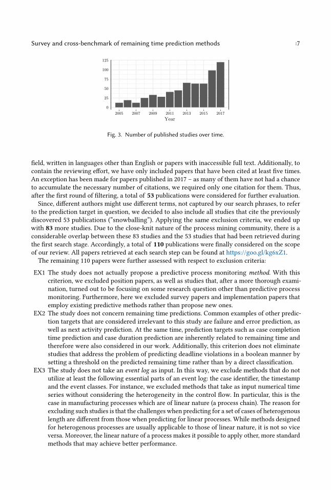
The initial search returned 670 unique results which is about 3 times more than the ones foundin [26], owing to the differences in search methodologies (Table 2). Figure 3 shows how the studiesare distributed over time. We can see that the interest in the topic of predictive process monitoringgrows over time with a sharp increase over the past few years.
Table 2. Comparison of our search methodology with [26]
Method in [26] Our method
Keywords 1. “predictive monitoring” AND 1. “predictive process”“business process” monitoring2. “business process” AND 2. “predictive business“prediction” process monitoring”
3. “predict (the) remaining time”4. “remaining time prediction”5. “predict (the) remaining * time”
Search scope Title, abstract, keywords Title, full textMin number of citations 5 (except 2016-2017 papers) 5 (except 2017 papers)Years covered 2010-2016 2005-2017Papers found after filtering 41 53Snowballing applied No Yes, one-hop
In order to consider only relevant studies, we designed a range of exclusion criteria to assessthe relevance of the studies. First, we excluded those papers not related to the process mining
Survey and cross-benchmark of remaining time prediction methods :7
0
25
50
75
100
125
2005 2007 2009 2011 2013 2015 2017Year
Fig. 3. Number of published studies over time.
field, written in languages other than English or papers with inaccessible full text. Additionally, tocontain the reviewing effort, we have only included papers that have been cited at least five times.An exception has been made for papers published in 2017 – as many of them have not had a chanceto accumulate the necessary number of citations, we required only one citation for them. Thus,after the first round of filtering, a total of 53 publications were considered for further evaluation.Since, different authors might use different terms, not captured by our search phrases, to refer
to the prediction target in question, we decided to also include all studies that cite the previouslydiscovered 53 publications (”snowballing”). Applying the same exclusion criteria, we ended upwith 83 more studies. Due to the close-knit nature of the process mining community, there is aconsiderable overlap between these 83 studies and the 53 studies that had been retrieved duringthe first search stage. Accordingly, a total of 110 publications were finally considered on the scopeof our review. All papers retrieved at each search step can be found at https://goo.gl/kg6xZ1.
The remaining 110 papers were further assessed with respect to exclusion criteria:
EX1 The study does not actually propose a predictive process monitoring method. With thiscriterion, we excluded position papers, as well as studies that, after a more thorough exami-nation, turned out to be focusing on some research question other than predictive processmonitoring. Furthermore, here we excluded survey papers and implementation papers thatemploy existing predictive methods rather than propose new ones.
EX2 The study does not concern remaining time predictions. Common examples of other predic-tion targets that are considered irrelevant to this study are failure and error prediction, aswell as next activity prediction. At the same time, prediction targets such as case completiontime prediction and case duration prediction are inherently related to remaining time andtherefore were also considered in our work. Additionally, this criterion does not eliminatestudies that address the problem of predicting deadline violations in a boolean manner bysetting a threshold on the predicted remaining time rather than by a direct classification.
EX3 The study does not take an event log as input. In this way, we exclude methods that do notutilize at least the following essential parts of an event log: the case identifier, the timestampand the event classes. For instance, we excluded methods that take as input numerical timeseries without considering the heterogeneity in the control flow. In particular, this is thecase in manufacturing processes which are of linear nature (a process chain). The reason forexcluding such studies is that the challenges when predicting for a set of cases of heterogenouslength are different from those when predicting for linear processes. While methods designedfor heterogenous processes are usually applicable to those of linear nature, it is not so viceversa. Moreover, the linear nature of a process makes it possible to apply other, more standardmethods that may achieve better performance.

:8 I. Verenich et al.
The application of the exclusion criteria resulted in 24 relevant studies which are described indetail in the following section.
4 ANALYSIS AND CLASSIFICATION OF METHODSDriven by the research questions defined in Section 3.1, we identified the following dimensions tocategorize and describe the relevant studies.
• Type of input data – RQ2• Awareness of the underlying business process – RQ2• Family of algorithms – RQ2• Type of evaluation data (real-life or artificial log) and application domain (e.g., insurance,banking, healthcare) – RQ3.• Type of implementation (standalone or plug-in, and tool accessibility) – RQ4
This information, summarized in Table 3, allows us to answer the first research question. In theremainder of this section, we proceed with surveying each main study method along the aboveclassification dimensions.
4.1 Input dataAs stipulated by EX3 criterion, all surveyed proposals take as input an event log. Such a log containsat least a case identifier, an activity and a timestamp. In addition, many techniques leverage caseand event attributes to make more accurate predictions. For example, in the pioneering predictivemonitoring approach described in [54], the authors predict the remaining processing time of a traceusing activity durations, their frequencies and various case attributes, such as the case priority.Many other approaches, e.g. [12], [36], [39] make use not only of case attributes but also of eventattributes, while applying one or more kinds of sequence encoding. Furthermore, some approaches,e.g. [18] and [39], exploit contextual information, such as workload indicators, to take into accountinter-case dependencies due to resource contention and data sharing. Finally, a group of works,e.g. [27] and [55] also leverage a process model in order to “replay” ongoing process cases on it.Such works treat remaining time as a cumulative indicator composed of cycle times of elementaryprocess components.
4.2 Process awarenessExisting techniques can be categorized according to their process-awareness, i.e. whether or notthe methodology exploits an explicit representation of a process model to make predictions. As canbe seen from Table 3, nearly a half of the techniques are process-aware. Most of them construct atransition system from an event log using set, bag (multiset) or sequence abstractions of observedevents. State transition systems are based on the idea that the process is composed of a set ofconsistent states and the movement between them [51]. Thus, a process behavior can be predictedif we know its current and future states.
Bolt and Sepúlveda [5] exploit query catalogs to store the information about the process behavior.Such catalogs are groups of partial traces (annotated with additional information about each partialtrace) that have occurred in an event log, and are then used to estimate the remaining time of newexecutions of the process.Also queuing models can be used for prediction because if a process follows a queuing context
and queuing measures (e.g. arrival rate, departure rate) can be accurately estimated and fit theprocess actual execution, the movement of a queuing item can be reliably predicted. Queueingtheory and regression-based techniques are combined for delay prediction in [40, 41].

Survey and cross-benchmark of remaining time prediction methods :9
Table 3. Overview of the 24 relevant studies resulting from the search (ordered by year and author).
Study Year Input data Process-aware? Algorithm Domain Implementation
van Dongen et al. [54] 2008 event log No regression public administration ProM 5data
van der Aalst et al. [52] 2011 event log Yes transition system public administration ProM 5Folino et al. [18] 2012 event log No clustering logistics ProM
datacontextual information
Pika et al. [33] 2012 event log No stat analysis financial ProMdata
van der Spoel et al. [53] 2012 event log Yes process graph healthcare n/adata regression
Bevacqua et al. [4] 2013 event log No clustering losistics ProMdata regression
Bolt and Sepúlveda [5] 2013 event log Yes stat analysis telecom n/asimulated
Folino et al. [19] 2013 event log No clustering customer support n/adatacontextual information
Pika et al. [34] 2013 event log No stat analysis insurance ProMdata
Rogge-Solti and Weske [37] 2013 event log Yes stoch Petri net logistics ProMdata simulated
Ceci et al. [7] 2014 event log Yes sequence trees customer service ProMdata regression workflow management
Folino et al. [20] 2014 event log No clustering logistics Nodata regression software developmentcontextual information
de Leoni et al. [11] 2014 event log No regression no validation ProMdatacontextual information
Polato et al. [35] 2014 event log Yes transition system public administration ProMdata regression
classificationSenderovich et al. [40] 2014 event log Yes queueing theory financial n/a
transition systemMetzger et al. [27] 2015 event log Yes neural network logistics n/a
data constraint satisfactionprocess model QoS aggregation
Rogge-Solti and Weske [38] 2015 event log Yes stoch Petri net financial ProMdata logistics
Senderovich et al. [41] 2015 event log Yes queueing theory financial n/atransition system telecom
Cesario et al. [8] 2016 event log Yes clustering logistics n/adata regression
de Leoni et al. [12] 2016 event log No regression no validation ProMdatacontextual information
Polato et al. [36] 2016 event log Yes transition system public administration ProMdata regression customer service
classificationSenderovich et al. [39] 2017 event log No regression healthcare standalone
data manufacturingcontextual information
Tax et al. [45] 2017 event log No neural network customer support standalonepublic administrationfinancial
Verenich et al. [55] 2017 event log Yes regression customer service standalonedata classification financialprocess model flow analysis
Furthermore, some process-aware approaches rely on stochastic Petri nets [37, 38] and processmodels in BPMN notation [55].
4.3 Family of algorithmsNon-process aware approaches typically rely on machine learning algorithms to make predictions.In particular, these algorithms take as input labeled training data in the form of feature vectors andthe corresponding labels. In case of remaining time predictions, these labels are continuous. Assuch, various regression methods can be utilized, such as regression trees [11, 12] or ensemble oftrees, i.e. random forest [53] and XGBoost [39].

:10 I. Verenich et al.
An emerging family of algorithms for predictive monitoring are artificial neural networks. Theyconsist of one layer of input units, one layer of output units, and multiple layers in-between whichare referred to as hidden units. While traditional machine learning methods heavily depend on thechoice of features on which they are applied, neural networks are capable of translating the datainto a compact intermediate representation to aid a hand-crafted feature engineering process [1]. Afeedforward network has been applied in [27] to predict deadline violations. More sophisticatedarchitectures based on recurrent neural networks were explored in [45].
Other approaches apply trace clustering to group similar traces to fit a predictive model for eachcluster. Then for any new running process case, predictions are made by using the predictor of thecluster it is estimated to belong to. Such approach is employed e.g., in [18] and [20].Another range of proposals utilizes statistical methods without training an explicit machine
learning model. For example, Pika et al. [33, 34] make predictions about time-related process risks byidentifying and leveraging process risk indicators (e.g., abnormal activity execution time or multipleactivity repetition) by applying statistical methods to event logs. The indicators are then combinedby means of a prediction function, which allows for highlighting the possibility of transgressingdeadlines. Conversely, Bolt and Sepúlveda [5] calculate remaining time based on the average timein the catalog which the partial trace belongs to, without taking into account distributions andconfidence intervals.
Rogge-Solti andWeske [37] mine a stochastic Petri net from the event log to predict the remainingtime of a case using arbitrary firing delays. The remaining time is evaluated based on the factthat there is an initial time distribution for a case to be executed. As inputs, the method receivesthe Petri net, the ongoing trace of the process instance up to current time, the current time andthe number of simulation iterations. The algorithm returns the average of simulated completiontimes of each iteration. This approach is extended in [38] to exploit the elapsed time since the lastobserved event to make more accurate predictions.Finally, Verenich et al. [55] propose a hybrid approach that relies on classification methods to
predict routing probabilities for each decision point in a process model, regression methods topredict cycle times of future events, and flow analysis methods to calculate the total remaining time.A conceptually similar approach is proposed by Polato et al. [36] who build a transition systemfrom an event log and enrich it with classification and regression models. Naive Bayes classifiersare used to estimate the probability of transition from one state to the other, while support vectorregressors are used to predict the remaining time from the next state.
4.4 Evaluation data and domainsAs reported in Table 3, most of the surveyed methods have been validated on at least one real-lifeevent log. Some studies were additionally validated on simulated (synthetic) logs.Importantly, many of the real-life logs are publicly available from the 4TU Center for Research
Data.2 Among the methods that employ real-life logs, we observed a growing trend to use publicly-available logs, as opposed to private logs which hinder the reproducibility of the results due to notbeing accessible.
Concerning the application domains of the real-life logs, we noticed that most of them pertain tologistics, banking (7 studies each), public administration (5 studies) and customer service (3 studies)processes.
2https://data.4tu.nl/repository/collection:event_logs_real

Survey and cross-benchmark of remaining time prediction methods :11
4.5 ImplementationNearly a half of the methods provide an implementation as a plug-in for the ProM framework.3 Thereason behind the popularity of ProM can be explained by its open-source and portable framework,which allows researchers to easily develop and test new algorithms. Also, ProM is historically thefirst process mining platform. Another three methods have a standalone implementation in Python.4 Finally, 8 methods do not provide a publicly available implementation.
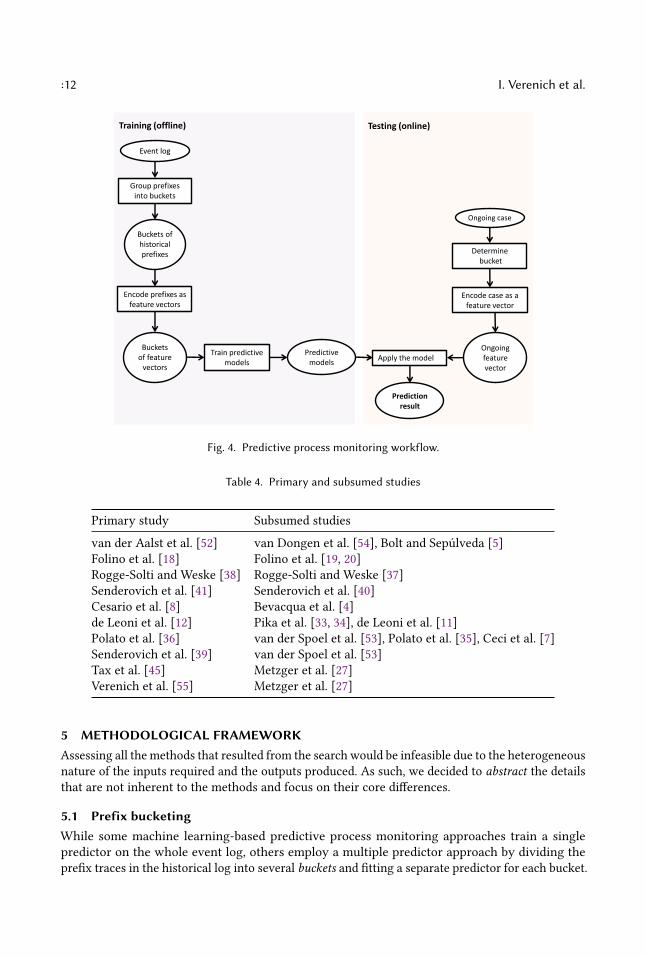
4.6 Predictive monitoring workflowAs indicated in Table 3, most predictive monitoring methods make use of machine learning al-gorithms based on regression, classification or neural networks. Such methods typically proceedin two phases: offline, to train a prediction model based on historical cases, and online, to makepredictions on running process cases (Figure 4) [48].In the offline phase, given an event log, case prefixes are extracted and filtered, e.g. to retain
only prefixes up to a certain length, to create a prefix log (cf. Section 2). Next, ”similar” prefixes aregrouped into homogeneous buckets, e.g. based on process states or similarities among prefixes andprefixes from each bucket are encoded into feature vectors. Then feature vectors from each bucketare used to fit a machine learning model.In the online phase, the actual predictions for running cases are made, by reusing the buckets,
encoders and predictive models built in the offline phase. Specifically, given a running case and aset of buckets of historical prefixes, the correct bucket is first determined. Next, this information isused to encode the features of the running case. In the last step, a prediction is extracted from theencoded case using the pre-trained model corresponding to the determined bucket.
Similar observations can be made for non-machine learning-based methods. For example, in [52]first, a transition system is derived and annotated and then the actual predictions are calculatedfor running cases. In principle, this transition system akin to a predictive model can be mined inadvance and used at runtime.
4.7 Primary and subsumed (related) studiesAmong the papers that successfully passed both the inclusion and exclusion criteria, we determinedprimary studies that constitute an original contribution for the purposes of our benchmark, andsubsumed studies that are similar to one of the primary studies and do not provide a substantialcontribution with respect to it.
Specifically, a study is considered subsumed if:• there exists a more recent and/or more extensive version of the study from the same authors(e.g. a conference paper is subsumed by an extended journal version), or• it does not propose a substantial improvement/modification over a method that is documentedin an earlier paper by other authors, or• the main contribution of the paper is a case study or a tool implementation, rather than thepredictive process monitoring method itself, and the method is described and/or evaluatedmore extensively in a more recent study by other authors.
This procedure resulted in 10 primary and 14 subsumed studies, as reported in Table 4. Somestudies are subsumed by several primary studies. For instance, Metzger et al. [27] use a feedforwardneural network which is subsumed by a more sophisticated recurrent neural network architectureextensively studied in [45]. At the same time, [27] describes a QoS technique which is subsumedby the flow analysis technique presented in [55].3http://promtools.org4https://www.python.org
:12 I. Verenich et al.
Event log
Encode prefixes as feature vectors
Train predictive models
Training (offline) Testing (online)
Buckets of feature
vectors
Predictive models
Encode case as a feature vector
Ongoing feature vector
Prediction result
Apply the model
Ongoing case
Group prefixes into buckets
Buckets of historical prefixes Determine
bucket
Fig. 4. Predictive process monitoring workflow.
Table 4. Primary and subsumed studies
Primary study Subsumed studies
van der Aalst et al. [52] van Dongen et al. [54], Bolt and Sepúlveda [5]Folino et al. [18] Folino et al. [19, 20]Rogge-Solti and Weske [38] Rogge-Solti and Weske [37]Senderovich et al. [41] Senderovich et al. [40]Cesario et al. [8] Bevacqua et al. [4]de Leoni et al. [12] Pika et al. [33, 34], de Leoni et al. [11]Polato et al. [36] van der Spoel et al. [53], Polato et al. [35], Ceci et al. [7]Senderovich et al. [39] van der Spoel et al. [53]Tax et al. [45] Metzger et al. [27]Verenich et al. [55] Metzger et al. [27]
5 METHODOLOGICAL FRAMEWORKAssessing all the methods that resulted from the search would be infeasible due to the heterogeneousnature of the inputs required and the outputs produced. As such, we decided to abstract the detailsthat are not inherent to the methods and focus on their core differences.
5.1 Prefix bucketingWhile some machine learning-based predictive process monitoring approaches train a singlepredictor on the whole event log, others employ a multiple predictor approach by dividing theprefix traces in the historical log into several buckets and fitting a separate predictor for each bucket.

Survey and cross-benchmark of remaining time prediction methods :13
To this end, Teinemaa et al. [48] surveyed several bucketing methods out of which three have beenutilized in the primary methods:
• Zero bucketing. All prefix traces are considered to be in the same bucket. As such, a singlepredictor is fit for all prefixes in the prefix log. This approach has been used in [12], [39] and[45].• Prefix length bucketing. Each bucket contains the prefixes of a specific length. For example,the n-th bucket contains prefixes where at least n events have been performed. One classifieris built for each possible prefix length. This approach has been used in [55].• Cluster bucketing. Here, each bucket represents a cluster that results from applying a clus-tering algorithm on the encoded prefixes. One classifier is trained for each resulting cluster,considering only the historical prefixes that fall into that particular cluster. At runtime, thecluster of the running case is determined based on its similarity to each of the existing clustersand the corresponding classifier is applied. This approach has been used in [18] and [8]• State bucketing. It is used in process-aware approaches where some kind of process represen-tation, e.g. in the form of a transition system, is derived and a predictor is trained for eachstate, or decision point. At runtime, the current state of the running case is determined, andthe respective predictor is used to make a prediction for the running case. This approach hasbeen used in [36].
5.2 Prefix encodingIn order to train a machine learning model, all prefixes in a given bucket need to be represented,or encoded as fixed-size feature vectors. Case attributes are static and their number is fixed for agiven process. Conversely, with each executed event, more information about the case becomesavailable. As such, the number of event attributes will increase over time. To address this issue,various sequence encoding techniques were proposed in related work summarized in [24] andrefined in [48]. In the primary studies, the following encoding techniques can be found:
• Last state encoding. In this encoding method, only event attributes of the lastm events areconsidered. Therefore, the size of the feature vector is proportional to the number of eventattributes and is fixed throughout the execution of a case.m = 1 is the most common choiceused, e.g. in [36], although in principle higherm values can also be used.• Aggregation encoding. In contrast to the last state encoding, all events since the beginning ofthe case are considered. However, to keep the feature vector size constant, various aggregationfunctions are applied to the values taken by a specific attribute throughout the case lifetime.For numeric attributes, common aggregation functions are minimum, average, maximum andsum of observed values, while for categorical ones count is generally used, e.g. the number oftimes a specific activity has been executed, or the number of activities a specific resource hasperformed [12].• Index-based encoding. Here for each position n in a prefix, we concatenate the event enoccurring in that position and the value of each event attribute in that position v1
n , . . . ,vkn ,
where k is the total number of attributes of an event. This type of encoding is lossless, i.e.it is possible to recover the original prefix based on its feature vector. On the other hand,with longer prefixes, it significantly increases the dimensionality of the feature vectors andhinders the model training process. This approach has been used in [55].• Tensor encoding. A tensor is a generalization of vectors and matrices to potentially higherdimensions [43]. Unlike conventional machine learning algorithms, tensor-based models donot require input to be encoded in a two-dimensional n ×m form, where n is the numberof training instances andm is the number of features. Conversely, they can take as input

:14 I. Verenich et al.
a three-dimensional tensor of shape n × t × p , where t is the number of events and p isthe number of event attributes, or features derived from each event. In other words, eachprefix is represented as a matrix where rows correspond to events and columns to featuresfor a given event. The data for each event is encoded ”as-is”. Case attributes are encodedas event attributes having the same value throughout the prefix. Hence, the encoding forLSTM is similar to the index-based encoding except for two differences: (i) case attributes areduplicated for each event, (ii) the feature vector is reshaped into a matrix.
To aid the explanation of the encoding types, Tables 5 – 7 provide examples of feature vectorsderived from the event log in Table 1. Note that for the index-based encoding, each trace σ in theevent log produces only one training sample per bucket, while the other encodings produce asmany samples as many prefixes can be derived from the original trace, i.e. up to |σ |.
Table 5. Feature vectors created from the log in Table 1 using last state encoding.
Channel Age Activity_last Time_last Resource_last Cost_lastEmail 37 A 0 John 15Email 37 B 80 Mark 25Email 37 D 180 Mary 10Email 37 F 305 Kate 20Email 37 G 350 John 20Email 37 H 360 Kate 15
Email 52 A 0 John 25Email 52 D 300 Mary 25Email 52 B 57900 Mark 10Email 52 F 58010 Kate 15
Table 6. Feature vectors created from the log in Table 1 using aggregated encoding.
ChannelAge Activ_AActiv_B Activ_DActiv_F Activ_GActiv_H Res_John Res_MarkRes_MaryRes_Kate sum_Time sum_Cost . . .
Email 37 1 0 0 0 0 0 1 0 0 0 0 15Email 37 1 1 0 0 0 0 1 1 0 0 80 40Email 37 1 1 1 0 0 0 1 1 1 0 180 50Email 37 1 1 1 1 0 0 1 1 1 1 305 70Email 37 1 1 1 1 1 0 2 1 1 1 350 90Email 37 1 1 1 1 1 1 2 1 1 2 360 105
Email 52 1 0 0 0 0 0 1 0 0 0 0 25Email 52 1 0 1 0 0 0 1 0 1 0 300 50Email 52 1 1 1 0 0 0 1 1 1 0 57900 60Email 52 1 1 1 1 0 0 1 1 1 1 58010 75
Table 7. Feature vectors created from the log in Table 1 using index-based encoding, buckets of length n = 3.
Channel Age Activ_1 Time_1 Res_1 Cost_1 Activ_2 Time_2 Res_2 Cost_2 Activ_3 Time_3 Res_3 Cost_3Email 37 A 0 John 15 B 80 Mark 25 D 180 Mary 10
Email 52 A 0 John 25 D 300 Mary 25 B 57900 Mark 10
These three ”canonical” encodings can serve as a basis for various modifications thereof. Forexample, de Leoni et al. [12] proposed the possibility of combining last state and aggregationencodings.
While the encoding techniques stipulate how to incorporate event attributes in a feature vector,the inclusion of case attributes and inter-case metrics, such as the number of currently open cases,is rather straightforward, as their number is fixed throughout the case lifetime.

Survey and cross-benchmark of remaining time prediction methods :15
While last state and aggregation encodings can be combined with any of the bucketing methodsdescribed in Section 5.1, index-based encoding is commonly used with prefix-length bucketing,as the feature vector size depends on the trace length [24]. Nevertheless, two options have beenproposed in related work to combine index-based encoding with other bucketing types:
• Fix the maximum prefix length and, for shorter prefixes, impute missing event attributevalues with zeros or their historical averages. This approach is often referred to as paddingin machine learning [42] and has been used in the context of predictive process monitoringin [46] and [29].• Use the sliding window method to encode only recent (up-to window sizew) history of theprefix. This approach has been proposed in [39].
5.3 Predictive algorithmsMachine learning-based predictive process monitoring methods have employed a variety of classi-fication and regression algorithms, with the most popular choice being decision trees (e.g. [12, 20]).Although quite simple, decision trees have an advantage in terms of computation performanceand interpretability of the results. Other choices include random forest [39, 55], support vectorregression [36] and extreme gradient boosting [39].A recent cross-benchmark of 13 state-of-the-art commonly used machine learning algorithms
on a set of 165 publicly available classification problems [31] found that gradient tree boostinggenerally achieves better accuracy than random forest, while random forest is more accurate thandecision trees. As a result, predictive process monitoring methods using predictive algorithms thatare inherently more accurate will perform better.In order to eliminate the bias associated with the usage of different predictors in related work,
we decided to fix extreme gradient boosting (XGBoost) [9] as the main predictor across all thecompared techniques. XGBoost is based on the theory of boosting, wherein the predictions ofseveral “weak” learners (models whose predictions are slightly better than random guessing), arecombined to produce a “strong” learner [21]. These “weak” learners are combined by followinga gradient learning strategy. At the beginning of the calibration process, a “weak” learner is fitto the whole space of data, and then, a second learner is fit to the residuals of the first one. Thisprocess of fitting a model to the residuals of the previous one goes on until some stopping criterionis reached. Finally, the output of XGBoost is a weighted mean of the individual predictions of eachweak learner. Regression trees are typically selected as “weak” learners [49].
Nevertheless, we set aside long short term memory (LSTM) neural networks as another predictorapplied in the primary method [45]. We will apply a zero bucketing with LSTMs, i.e. train a singleLSTM model for all prefixes, as this is the only bucketing type that has been used with LSTMsin the literature. As unlike other predictors, LSTMs do not require flattening the input data, wewill naturally use tensor encoding with them. Similarly to the other predictors, to overcome theproblem of feature vectors increasing with the prefix size, we fix the maximum number of eventsin the prefix (cf. Section 6.2.2) and for shorter prefixes, pad the data for missing events with zerosas in [29, 46].
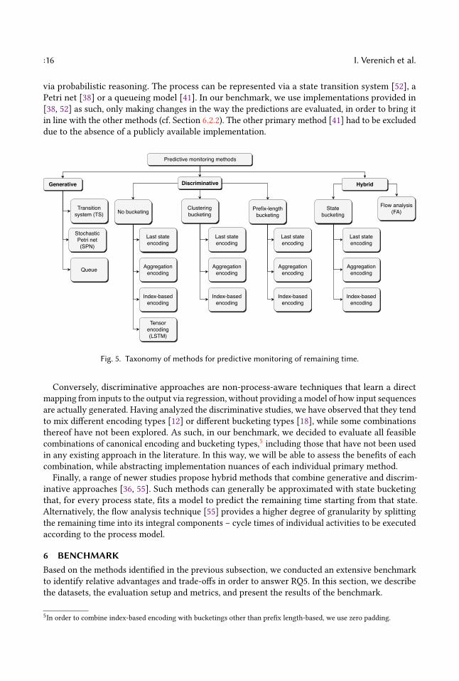
5.4 DiscussionSummarizing the above observations, we devised a taxonomy of predictive monitoring techniquesto be evaluated in our cross-benchmark (Figure 5). The taxonomy is framed upon a general classifi-cation of machine learning approaches into generative and discriminative ones (cf. Section 2.2).
The former correspond to process-aware predictive monitoring techniques, meaning that there isan assumption that an observed sequence is generated by some process that needs to be uncovered
:16 I. Verenich et al.
via probabilistic reasoning. The process can be represented via a state transition system [52], aPetri net [38] or a queueing model [41]. In our benchmark, we use implementations provided in[38, 52] as such, only making changes in the way the predictions are evaluated, in order to bring itin line with the other methods (cf. Section 6.2.2). The other primary method [41] had to be excludeddue to the absence of a publicly available implementation.
Predictive monitoring methods
DiscriminativeGenerative Hybrid
Transitionsystem (TS)
StochasticPetri net(SPN)
Queue
No bucketing
Last stateencoding
Aggregationencoding
Index-basedencoding
Clusteringbucketing
Last stateencoding
Aggregationencoding
Index-basedencoding
Prefix-lengthbucketing
Last stateencoding
Aggregationencoding
Index-basedencoding
Statebucketing
Flow analysis(FA)
Last stateencoding
Aggregationencoding
Index-basedencoding
Tensorencoding(LSTM)
Fig. 5. Taxonomy of methods for predictive monitoring of remaining time.
Conversely, discriminative approaches are non-process-aware techniques that learn a directmapping from inputs to the output via regression, without providing amodel of how input sequencesare actually generated. Having analyzed the discriminative studies, we have observed that they tendto mix different encoding types [12] or different bucketing types [18], while some combinationsthereof have not been explored. As such, in our benchmark, we decided to evaluate all feasiblecombinations of canonical encoding and bucketing types,5 including those that have not been usedin any existing approach in the literature. In this way, we will be able to assess the benefits of eachcombination, while abstracting implementation nuances of each individual primary method.
Finally, a range of newer studies propose hybrid methods that combine generative and discrim-inative approaches [36, 55]. Such methods can generally be approximated with state bucketingthat, for every process state, fits a model to predict the remaining time starting from that state.Alternatively, the flow analysis technique [55] provides a higher degree of granularity by splittingthe remaining time into its integral components – cycle times of individual activities to be executedaccording to the process model.
6 BENCHMARKBased on the methods identified in the previous subsection, we conducted an extensive benchmarkto identify relative advantages and trade-offs in order to answer RQ5. In this section, we describethe datasets, the evaluation setup and metrics, and present the results of the benchmark.
5In order to combine index-based encoding with bucketings other than prefix length-based, we use zero padding.
Survey and cross-benchmark of remaining time prediction methods :17
6.1 DatasetsWe conducted the experiments using 16 real-life event datasets. To ensure the reproducibility ofthe experiments, the logs we used are publicly available at the 4TU Center for Research Data6 as ofMarch 2018, except for one log, which we obtained from the demonstration version of a softwaretool.We excluded from the evaluation those logs that do not pertain to business processes (e.g.,
JUnit 4.12 Software Event Log and NASA Crew Exploration Vehicle). Such logs are usually notcase-based or they contain only a few cases. Furthermore, we discarded the log that comes fromthe Environmental permit application process, as it is an earlier version of the BPIC 2015 event logfrom the same collection.All the logs have been preprocessed beforehand to ensure the maximum achievable prediction
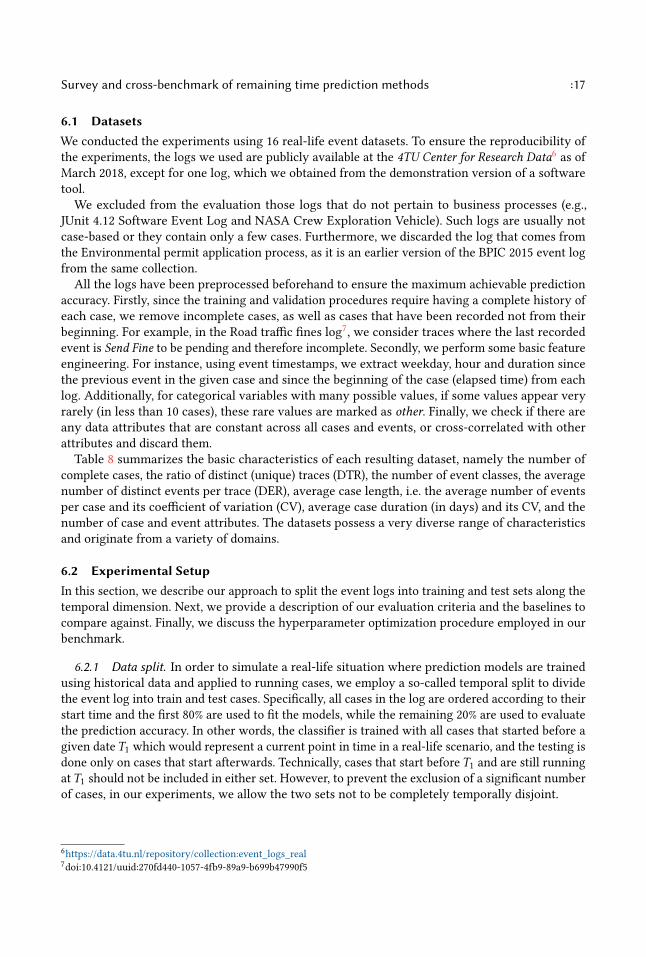
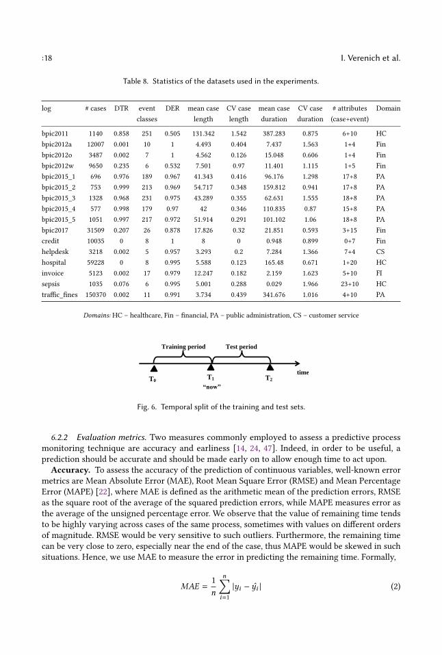
accuracy. Firstly, since the training and validation procedures require having a complete history ofeach case, we remove incomplete cases, as well as cases that have been recorded not from theirbeginning. For example, in the Road traffic fines log7, we consider traces where the last recordedevent is Send Fine to be pending and therefore incomplete. Secondly, we perform some basic featureengineering. For instance, using event timestamps, we extract weekday, hour and duration sincethe previous event in the given case and since the beginning of the case (elapsed time) from eachlog. Additionally, for categorical variables with many possible values, if some values appear veryrarely (in less than 10 cases), these rare values are marked as other. Finally, we check if there areany data attributes that are constant across all cases and events, or cross-correlated with otherattributes and discard them.Table 8 summarizes the basic characteristics of each resulting dataset, namely the number of
complete cases, the ratio of distinct (unique) traces (DTR), the number of event classes, the averagenumber of distinct events per trace (DER), average case length, i.e. the average number of eventsper case and its coefficient of variation (CV), average case duration (in days) and its CV, and thenumber of case and event attributes. The datasets possess a very diverse range of characteristicsand originate from a variety of domains.
6.2 Experimental SetupIn this section, we describe our approach to split the event logs into training and test sets along thetemporal dimension. Next, we provide a description of our evaluation criteria and the baselines tocompare against. Finally, we discuss the hyperparameter optimization procedure employed in ourbenchmark.
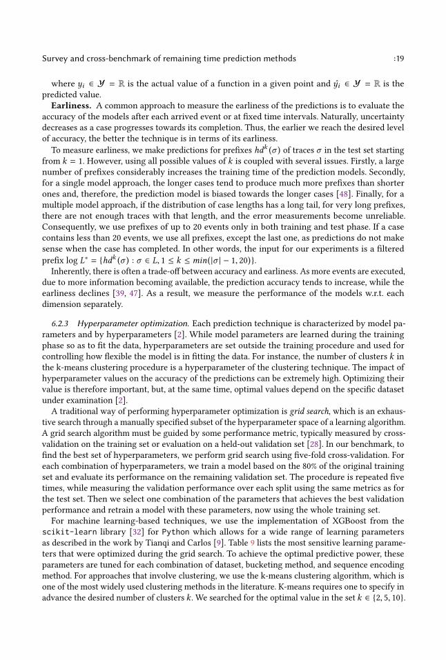
6.2.1 Data split. In order to simulate a real-life situation where prediction models are trainedusing historical data and applied to running cases, we employ a so-called temporal split to dividethe event log into train and test cases. Specifically, all cases in the log are ordered according to theirstart time and the first 80% are used to fit the models, while the remaining 20% are used to evaluatethe prediction accuracy. In other words, the classifier is trained with all cases that started before agiven dateT1 which would represent a current point in time in a real-life scenario, and the testing isdone only on cases that start afterwards. Technically, cases that start beforeT1 and are still runningatT1 should not be included in either set. However, to prevent the exclusion of a significant numberof cases, in our experiments, we allow the two sets not to be completely temporally disjoint.
6https://data.4tu.nl/repository/collection:event_logs_real7doi:10.4121/uuid:270fd440-1057-4fb9-89a9-b699b47990f5
:18 I. Verenich et al.
Table 8. Statistics of the datasets used in the experiments.
log # cases DTR event DER mean case CV case mean case CV case # attributes Domainclasses length length duration duration (case+event)
bpic2011 1140 0.858 251 0.505 131.342 1.542 387.283 0.875 6+10 HCbpic2012a 12007 0.001 10 1 4.493 0.404 7.437 1.563 1+4 Finbpic2012o 3487 0.002 7 1 4.562 0.126 15.048 0.606 1+4 Finbpic2012w 9650 0.235 6 0.532 7.501 0.97 11.401 1.115 1+5 Finbpic2015_1 696 0.976 189 0.967 41.343 0.416 96.176 1.298 17+8 PAbpic2015_2 753 0.999 213 0.969 54.717 0.348 159.812 0.941 17+8 PAbpic2015_3 1328 0.968 231 0.975 43.289 0.355 62.631 1.555 18+8 PAbpic2015_4 577 0.998 179 0.97 42 0.346 110.835 0.87 15+8 PAbpic2015_5 1051 0.997 217 0.972 51.914 0.291 101.102 1.06 18+8 PAbpic2017 31509 0.207 26 0.878 17.826 0.32 21.851 0.593 3+15 Fincredit 10035 0 8 1 8 0 0.948 0.899 0+7 Finhelpdesk 3218 0.002 5 0.957 3.293 0.2 7.284 1.366 7+4 CShospital 59228 0 8 0.995 5.588 0.123 165.48 0.671 1+20 HCinvoice 5123 0.002 17 0.979 12.247 0.182 2.159 1.623 5+10 FIsepsis 1035 0.076 6 0.995 5.001 0.288 0.029 1.966 23+10 HCtraffic_fines 150370 0.002 11 0.991 3.734 0.439 341.676 1.016 4+10 PA
Domains: HC – healthcare, Fin – financial, PA – public administration, CS – customer service
T1
Test period Training period
time T0 T2
j
i
“now”
Fig. 6. Temporal split of the training and test sets.
6.2.2 Evaluation metrics. Two measures commonly employed to assess a predictive processmonitoring technique are accuracy and earliness [14, 24, 47]. Indeed, in order to be useful, aprediction should be accurate and should be made early on to allow enough time to act upon.
Accuracy. To assess the accuracy of the prediction of continuous variables, well-known errormetrics are Mean Absolute Error (MAE), Root Mean Square Error (RMSE) and Mean PercentageError (MAPE) [22], where MAE is defined as the arithmetic mean of the prediction errors, RMSEas the square root of the average of the squared prediction errors, while MAPE measures error asthe average of the unsigned percentage error. We observe that the value of remaining time tendsto be highly varying across cases of the same process, sometimes with values on different ordersof magnitude. RMSE would be very sensitive to such outliers. Furthermore, the remaining timecan be very close to zero, especially near the end of the case, thus MAPE would be skewed in suchsituations. Hence, we use MAE to measure the error in predicting the remaining time. Formally,
MAE =1n
n∑i=1|yi − yi | (2)
Survey and cross-benchmark of remaining time prediction methods :19
where yi ∈ Y = R is the actual value of a function in a given point and yi ∈ Y = R is thepredicted value.
Earliness. A common approach to measure the earliness of the predictions is to evaluate theaccuracy of the models after each arrived event or at fixed time intervals. Naturally, uncertaintydecreases as a case progresses towards its completion. Thus, the earlier we reach the desired levelof accuracy, the better the technique is in terms of its earliness.
To measure earliness, we make predictions for prefixes hdk (σ ) of traces σ in the test set startingfrom k = 1. However, using all possible values of k is coupled with several issues. Firstly, a largenumber of prefixes considerably increases the training time of the prediction models. Secondly,for a single model approach, the longer cases tend to produce much more prefixes than shorterones and, therefore, the prediction model is biased towards the longer cases [48]. Finally, for amultiple model approach, if the distribution of case lengths has a long tail, for very long prefixes,there are not enough traces with that length, and the error measurements become unreliable.Consequently, we use prefixes of up to 20 events only in both training and test phase. If a casecontains less than 20 events, we use all prefixes, except the last one, as predictions do not makesense when the case has completed. In other words, the input for our experiments is a filteredprefix log L∗ = {hdk (σ ) : σ ∈ L, 1 ≤ k ≤ min( |σ | − 1, 20)}.
Inherently, there is often a trade-off between accuracy and earliness. As more events are executed,due to more information becoming available, the prediction accuracy tends to increase, while theearliness declines [39, 47]. As a result, we measure the performance of the models w.r.t. eachdimension separately.
6.2.3 Hyperparameter optimization. Each prediction technique is characterized by model pa-rameters and by hyperparameters [2]. While model parameters are learned during the trainingphase so as to fit the data, hyperparameters are set outside the training procedure and used forcontrolling how flexible the model is in fitting the data. For instance, the number of clusters k inthe k-means clustering procedure is a hyperparameter of the clustering technique. The impact ofhyperparameter values on the accuracy of the predictions can be extremely high. Optimizing theirvalue is therefore important, but, at the same time, optimal values depend on the specific datasetunder examination [2].
A traditional way of performing hyperparameter optimization is grid search, which is an exhaus-tive search through a manually specified subset of the hyperparameter space of a learning algorithm.A grid search algorithm must be guided by some performance metric, typically measured by cross-validation on the training set or evaluation on a held-out validation set [28]. In our benchmark, tofind the best set of hyperparameters, we perform grid search using five-fold cross-validation. Foreach combination of hyperparameters, we train a model based on the 80% of the original trainingset and evaluate its performance on the remaining validation set. The procedure is repeated fivetimes, while measuring the validation performance over each split using the same metrics as forthe test set. Then we select one combination of the parameters that achieves the best validationperformance and retrain a model with these parameters, now using the whole training set.For machine learning-based techniques, we use the implementation of XGBoost from the
scikit-learn library [32] for Python which allows for a wide range of learning parametersas described in the work by Tianqi and Carlos [9]. Table 9 lists the most sensitive learning parame-ters that were optimized during the grid search. To achieve the optimal predictive power, theseparameters are tuned for each combination of dataset, bucketing method, and sequence encodingmethod. For approaches that involve clustering, we use the k-means clustering algorithm, which isone of the most widely used clustering methods in the literature. K-means requires one to specify inadvance the desired number of clusters k . We searched for the optimal value in the set k ∈ {2, 5, 10}.

:20 I. Verenich et al.
In the case of the index-based bucketing method, an optimal configuration was chosen for eachprefix length separately.
Table 9. Hyperparameters tuned via grid search.
Parameter Explanation Search spaceXGBoost
n_estimators Number of decision trees (“weak” learners) in the ensemble {250, 500}learning_rate Shrinks the contribution of each successive decision tree in the ensemble {0.02, 0.04, 0.06}subsample Fraction of observations to be randomly sampled for each tree. {0.5, 0.8}colsample_bytree Fraction of columns (features) to be randomly sampled for each tree. {0.5, 0.8}max_depth Maximum tree depth for base learners {3, 6}
LSTMunits Number of neurons per hidden layer {100, 200}n_layers Number of hidden layers {1, 2, 3}batch Number of samples to be propagated {8, 32}activation Activation function to use {ReLU }optimizer Weight optimizer {RMSprop,Nadam}
For LSTMs, we used the recurrent neural network library [10], with Tensorflow backend. Aswith XGBoost, we performed tuning using grid search using the parameters specified in Table 9.These parameters and their values were chosen based on the results reported in [45]. Otherhyperparameters were left to their defaults.A similar procedure is performed for methods that do not train a machine learning model. For
the method in [52], we vary the type of abstraction – set, bag of sequence – to create a transitionsystem. For the method in [38], we vary the stochastic Petri net properties: (i) the kind of transitiondistribution – normal, gaussian kernel or histogram and (ii) memory semantics – global preselectionor race with memory. We select the parameters that yield the best performance on the validationset and use them for the test set.
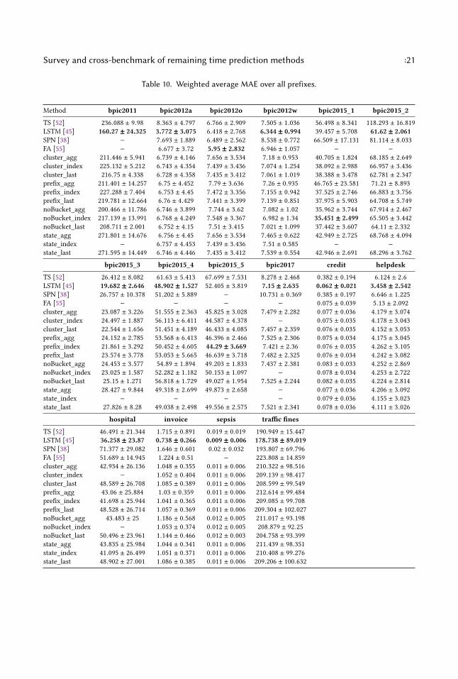
6.3 Evaluation resultsTable 10 reports the prediction accuracy, averaged across all evaluated prefix lengths, togetherwith its standard deviation. The averages are weighted by the relative frequency of prefixes withthat prefix (i.e. longer prefixes get lower weights, since not all traces reach that length). In ourexperiences, we set an execution cap of 6 hours for each training configuration, so if some methoddid not finish within that time, the corresponding cell in the Table is empty. Furthermore, sincethe flow-analysis approach [55] cannot readily deal with unstructured process models, we onlyprovide its results for the logs from which we were able to derive structured models.
Overall, we can see that in 13 out of 16 datasets, LSTM-based networks achieve the best accuracy,while flow-analysis and index-based encoding with no bucketing and prefix-length bucketingachieve the best results in one dataset each.
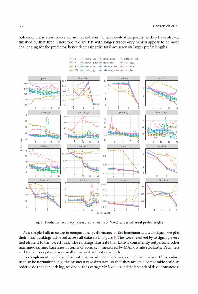
Figure 7 presents the prediction accuracy in terms of MAE, evaluated over different prefix lengths.Each evaluation point includes prefixes of exactly the given length. In other words, traces that areshorter than the required prefix are left out of the calculation. Therefore, the number of cases usedfor evaluation is monotonically decreasing when increasing the prefix length.In most of the datasets, we see that the MAE decreases as cases progress. It is natural that the
prediction task becomes trivial when cases are close to completion. However, for some datasets,the predictions become less accurate as the prefix length increases. This phenomenon is caused bythe fact that these datasets contain some short traces for which it appears to be easy to predict the
Survey and cross-benchmark of remaining time prediction methods :21
Table 10. Weighted average MAE over all prefixes.
Method bpic2011 bpic2012a bpic2012o bpic2012w bpic2015_1 bpic2015_2
TS [52] 236.088 ± 9.98 8.363 ± 4.797 6.766 ± 2.909 7.505 ± 1.036 56.498 ± 8.341 118.293 ± 16.819LSTM [45] 160.27 ± 24.325 3.772 ± 3.075 6.418 ± 2.768 6.344 ± 0.994 39.457 ± 5.708 61.62 ± 2.061SPN [38] − 7.693 ± 1.889 6.489 ± 2.562 8.538 ± 0.772 66.509 ± 17.131 81.114 ± 8.033FA [55] − 6.677 ± 3.72 5.95 ± 2.832 6.946 ± 1.057 − −
cluster_agg 211.446 ± 5.941 6.739 ± 4.146 7.656 ± 3.534 7.18 ± 0.953 40.705 ± 1.824 68.185 ± 2.649cluster_index 225.132 ± 5.212 6.743 ± 4.354 7.439 ± 3.436 7.074 ± 1.254 38.092 ± 2.988 66.957 ± 3.436cluster_last 216.75 ± 4.338 6.728 ± 4.358 7.435 ± 3.412 7.061 ± 1.019 38.388 ± 3.478 62.781 ± 2.347prefix_agg 211.401 ± 14.257 6.75 ± 4.452 7.79 ± 3.636 7.26 ± 0.935 46.765 ± 23.581 71.21 ± 8.893prefix_index 227.288 ± 7.404 6.753 ± 4.45 7.472 ± 3.356 7.155 ± 0.942 37.525 ± 2.746 66.883 ± 3.756prefix_last 219.781 ± 12.664 6.76 ± 4.429 7.441 ± 3.399 7.139 ± 0.851 37.975 ± 5.903 64.708 ± 5.749noBucket_agg 200.466 ± 11.786 6.746 ± 3.899 7.744 ± 3.62 7.082 ± 1.02 35.962 ± 3.744 67.914 ± 2.467noBucket_index 217.139 ± 13.991 6.768 ± 4.249 7.548 ± 3.367 6.982 ± 1.34 35.451 ± 2.499 65.505 ± 3.442noBucket_last 208.711 ± 2.001 6.752 ± 4.15 7.51 ± 3.415 7.021 ± 1.099 37.442 ± 3.607 64.11 ± 2.332state_agg 271.801 ± 14.676 6.756 ± 4.45 7.656 ± 3.534 7.465 ± 0.622 42.949 ± 2.725 68.768 ± 4.094state_index − 6.757 ± 4.453 7.439 ± 3.436 7.51 ± 0.585 − −
state_last 271.595 ± 14.449 6.746 ± 4.446 7.435 ± 3.412 7.539 ± 0.554 42.946 ± 2.691 68.296 ± 3.762
bpic2015_3 bpic2015_4 bpic2015_5 bpic2017 credit helpdesk
TS [52] 26.412 ± 8.082 61.63 ± 5.413 67.699 ± 7.531 8.278 ± 2.468 0.382 ± 0.194 6.124 ± 2.6LSTM [45] 19.682 ± 2.646 48.902 ± 1.527 52.405 ± 3.819 7.15 ± 2.635 0.062 ± 0.021 3.458 ± 2.542SPN [38] 26.757 ± 10.378 51.202 ± 5.889 − 10.731 ± 0.369 0.385 ± 0.197 6.646 ± 1.225FA [55] − − − − 0.075 ± 0.039 5.13 ± 2.092cluster_agg 23.087 ± 3.226 51.555 ± 2.363 45.825 ± 3.028 7.479 ± 2.282 0.077 ± 0.036 4.179 ± 3.074cluster_index 24.497 ± 1.887 56.113 ± 6.411 44.587 ± 4.378 − 0.075 ± 0.035 4.178 ± 3.043cluster_last 22.544 ± 1.656 51.451 ± 4.189 46.433 ± 4.085 7.457 ± 2.359 0.076 ± 0.035 4.152 ± 3.053prefix_agg 24.152 ± 2.785 53.568 ± 6.413 46.396 ± 2.466 7.525 ± 2.306 0.075 ± 0.034 4.175 ± 3.045prefix_index 21.861 ± 3.292 50.452 ± 4.605 44.29 ± 3.669 7.421 ± 2.36 0.076 ± 0.035 4.262 ± 3.105prefix_last 23.574 ± 3.778 53.053 ± 5.665 46.639 ± 3.718 7.482 ± 2.325 0.076 ± 0.034 4.242 ± 3.082noBucket_agg 24.453 ± 3.577 54.89 ± 1.894 49.203 ± 1.833 7.437 ± 2.381 0.083 ± 0.033 4.252 ± 2.869noBucket_index 23.025 ± 1.587 52.282 ± 1.182 50.153 ± 1.097 − 0.078 ± 0.034 4.253 ± 2.722noBucket_last 25.15 ± 1.271 56.818 ± 1.729 49.027 ± 1.954 7.525 ± 2.244 0.082 ± 0.035 4.224 ± 2.814state_agg 28.427 ± 9.844 49.318 ± 2.699 49.873 ± 2.658 − 0.077 ± 0.036 4.206 ± 3.092state_index − − − − 0.079 ± 0.036 4.155 ± 3.023state_last 27.826 ± 8.28 49.038 ± 2.498 49.556 ± 2.575 7.521 ± 2.341 0.078 ± 0.036 4.111 ± 3.026
hospital invoice sepsis traffic fines
TS [52] 46.491 ± 21.344 1.715 ± 0.891 0.019 ± 0.019 190.949 ± 15.447LSTM [45] 36.258 ± 23.87 0.738 ± 0.266 0.009 ± 0.006 178.738 ± 89.019SPN [38] 71.377 ± 29.082 1.646 ± 0.601 0.02 ± 0.032 193.807 ± 69.796FA [55] 51.689 ± 14.945 1.224 ± 0.51 − 223.808 ± 14.859cluster_agg 42.934 ± 26.136 1.048 ± 0.355 0.011 ± 0.006 210.322 ± 98.516cluster_index − 1.052 ± 0.404 0.011 ± 0.006 209.139 ± 98.417cluster_last 48.589 ± 26.708 1.085 ± 0.389 0.011 ± 0.006 208.599 ± 99.549prefix_agg 43.06 ± 25.884 1.03 ± 0.359 0.011 ± 0.006 212.614 ± 99.484prefix_index 41.698 ± 25.944 1.041 ± 0.365 0.011 ± 0.006 209.085 ± 99.708prefix_last 48.528 ± 26.714 1.057 ± 0.369 0.011 ± 0.006 209.304 ± 102.027noBucket_agg 43.483 ± 25 1.186 ± 0.568 0.012 ± 0.005 211.017 ± 93.198noBucket_index − 1.053 ± 0.374 0.012 ± 0.005 208.879 ± 92.25noBucket_last 50.496 ± 23.961 1.144 ± 0.466 0.012 ± 0.003 204.758 ± 93.399state_agg 43.835 ± 25.984 1.044 ± 0.341 0.011 ± 0.006 211.439 ± 98.351state_index 41.095 ± 26.499 1.051 ± 0.371 0.011 ± 0.006 210.408 ± 99.276state_last 48.902 ± 27.001 1.086 ± 0.385 0.011 ± 0.006 209.206 ± 100.632
:22 I. Verenich et al.
outcome. These short traces are not included in the later evaluation points, as they have alreadyfinished by that time. Therefore, we are left with longer traces only, which appear to be morechallenging for the predictor, hence decreasing the total accuracy on larger prefix lengths.
●
●
●
●
●
●
●
●
● ●● ●
●
●
● ●
● ●● ●
●
●
●
●
●●
●●
●●
● ●
●
●●
●
●
●
●
●
●
●
● ● ● ● ●● ● ● ● ● ● ●
● ● ● ● ● ●
●●
● ●●
●● ● ● ● ● ● ● ●
●● ●
● ● ●● ●
●
●
●●
●● ●
●● ●
●● ● ● ●
●● ●
●
●
●
●●
●
●
● ●●
●
● ● ●●
●
●●
● ●
●
●●
●● ● ●
● ●
● ● ●●
● ●● ● ● ●
●
●
●
●
●
●
●
●
●
●
●
●
●●
● ●● ● ●
●●
●
●●
● ● ●●
● ● ● ● ● ● ● ● ● ● ● ● ●
●
●
●●
● ● ●● ● ● ● ● ● ● ● ● ● ● ● ●
●
● ● ● ● ● ● ● ● ● ● ● ● ● ● ●● ● ● ●
●
●
●
●
● ●●
●
●●
●●
● ●
● ●
● ●●
●
●
●●
●
● ●●
●
●●
●●
● ●
● ●
● ●●
●
●●
● ●●
● ● ●
●●
● ●
● ●
● ●●
●
●●
●●
● ● ● ● ●● ● ●
● ●●
●●
●● ●
●
●
●
●● ● ● ● ●
●● ●
●
●
●
●
● ● ● ●
●●
●● ●
● ●● ●
● ● ●● ● ●
● ●
● ● ● ● ●
●
● ●●
● ●● ●
●●
●●
● ●●
● ● ● ● ●
● ● ●● ● ● ●
● ●● ● ●
●●
●● ● ● ● ●
●● ●
● ●● ●
● ●●
●
●
●
●
●
●
● ● ● ●
●
● ●●
● ●● ●
● ●●
●
● ●
● ● ● ● ● ●
●
●
●
●● ● ●
●●
●
●
●
●●
● ●● ●
●
●
● ● ●● ● ● ●
● ● ●● ● ● ●
●
● ● ● ● ●
●
● ●● ● ● ● ● ● ●
● ●● ●
●
● ● ●● ●
●
● ●● ● ● ●
● ● ●● ● ● ●
●● ● ● ● ●
●● ●
●
●●
●●
● ● ●● ●
●
●
● ● ● ●●
●●
● ●●
● ●● ●
● ●● ●
●
●
● ● ● ●●
●
●
●
●
●
●
●
●
●
●
● ●
●
●
●
● ●
●●
●●
●
●●
● ●● ●
●● ●
●
●
● ● ●●
●● ●
●
●
● ● ●●
● ● ●● ●
●●
●
●● ● ●
●●
●●
●
●
●
● ● ●
●● ● ●
●
●●
● ● ● ● ●
●●
●
●● ● ●
●
●● ● ●
● ● ● ● ● ● ●●
●
● ●●
●
● ●
●
●
●
● ●●
●
●● ●
● ●
●
●
● ●● ●
●
● ●●
●●
●●
●
●●
●●
●●
●
●●
●
●
●
●
●
●
●●
●
●
●
● ●
●
●
● ●
●
●
●
●●
●● ● ●
● ●● ●
● ●● ● ●
●●
●● ● ● ●
●●
● ●●
●
● ●● ● ● ● ● ● ●
● ● ● ● ● ● ● ● ● ●●
●●
● ● ●●
●
●●●
●
●
● ● ● ●
● ●●
●
● ●●
●
●
●
●● ●
●●
●
● ●
●●
●●
●●
●
●
●
●
●
●
●● ●
●
●
●●
● ●
●
●
● ● ●
●
●
●●
●
●
●
●
●
●
● ●
●
●
●●
●
●
●
●
● ●
●
●
●
●
●●
●
●
●
●
●
●
●
●
●
●
●
●
●
●
●
●
●
●
●
●
●
●
●
●
●
●
●
●
●
●
●
●
●
●
●●
●
●
●
●
●
●
●
●
● ●
●
●
●
● ●
●
●
●
●
●
●
●●
●
●
●
● ●
● ●
●
●
●
● ●
●
●
●
●
●
● ●
●
●
●
●●
● ●
●
●
●
●●
● ●
●
●
●
● ●
● ●
●
●
●
● ●
● ●
●
●
●
● ●
● ●
●
●
●
●●
● ●
●
●
●
● ●
● ●
●
●
●
●●
● ●
●
●
●
● ●
● ●
●
●
●
● ●
● ●
●
●
●
● ●
●
●
●
●
●
●
●
●
●
●
●
●
● ●
●
●
●
●●
●
●●
●●
●● ●
●● ●
●●
● ● ●●
●●
●●
●
●
●
● ●● ● ● ● ● ● ●
●●
● ●
● ● ● ●
●
●●
●● ● ●
● ● ●●
● ● ●● ● ● ● ● ●
●
● ●● ● ● ●
● ●● ●
●●
●
● ● ● ●● ●
●
● ● ● ● ●● ●
●
●
●●
●● ●
● ● ● ●●
●
● ●
●● ●
●●
●● ●
●
●
●
●
●
●●
●●
●
● ●●
● ●●
●
●
●
●
●
●● ●
●● ●
●●
●
●
●
● ●●
●
● ●
●
●
●
●
●
●● ●
●●
●
●
● ●● ●
●● ● ●
●●
● ●●
● ● ● ●● ●
●
● ●● ● ● ● ● ● ● ●
● ● ● ● ● ● ●● ●●
● ● ● ● ●●
● ● ● ●
● ●● ● ● ● ● ●
●
●
●
●●
● ● ● ● ●
●●
● ●
●
●
●●
● ● ●●
●
●
● ● ● ● ● ●
●●
●●
●
●
●●
● ● ●
●● ● ● ● ● ● ● ●
●
● ●
●
●●
●
●●
●
●
● ● ●
●
●
●
●● ●
●
●● ●
●
●
● ●●
●●
● ● ●
●
●● ● ● ●
●
●
●
● ● ●
●
●● ●
●
● ● ●
●
●
●●
● ●
●
●●
●
●●
●●
● ●●
● ● ●
●
●
●● ● ●
●
● ● ●
●
●
● ● ● ●●
● ● ●
●
●
● ●● ●
●
●●
●
●
●
●●
●●
●
● ● ●
●
●
●● ● ●
●
●●
●
●
● ●● ● ●
●
● ● ●
●
●
●● ● ●
●
●●
●
●
●● ●
● ●
●
● ● ●
●
●
●● ● ●
●
●●
●
●
●●
●● ●
●
● ● ●
●
●
● ● ● ●
●
● ● ●
●● ● ●
●● ●
● ● ●
●
●
●● ● ●
●
● ●●
●
●
●●
● ● ●
● ● ● ● ●●
●
●
●
●
●
●
●
●
●
● ● ● ● ● ●● ●
●
●
●
● ●
●
● ● ● ● ● ● ●●
●
● ●
●● ● ●
● ● ● ● ● ●● ●
●
●
●
●
● ●
●
● ● ● ● ● ● ●●
●
● ●
●
●
● ●
● ● ● ● ● ●●
●
●
● ●
●
●
● ●
● ● ● ●● ● ●
●
●
● ●
●
●
● ●
● ● ●●
●● ● ●
●
● ●
●
●●
●● ● ● ● ●
●●
●
●
● ●
●
●
●
●
● ● ● ● ●● ●
●
●
● ●
●
● ●
●
● ● ● ● ● ● ●●
●
● ●
●
●● ●
● ● ● ● ● ● ●●
●
● ●
●
● ● ●
● ● ● ● ● ● ●●
●
● ●
●
● ● ●
● ● ●●
● ● ●
●
●
● ●
●
●●
●
● ● ● ● ● ● ●●
●
● ●
●
●
●●
● ● ● ●●
●●
●
●
● ●
●
● ●
●
● ●
●
●
●
●
●
● ● ●
●
●
● ●
●
●
● ●
●
● ● ●
●
● ● ●
●
●
●
●
●
● ● ●
●
● ● ●
●
●
● ●
●
● ● ●
●
●● ●
●
●
● ●
●
● ● ●
●
● ● ●
●
●
●
●● ● ●
●●
● ●
●●
●● ● ●
●
●●
●
● ●
●●
● ●● ● ● ●
●● ●
● ● ● ● ●●
●
●
●
● ●●
●
●
● ●●
●●
●● ● ● ● ●
●
●
● ● ●
● ●● ● ●
●● ● ● ●
●●
●● ● ●
●
● ● ● ● ●● ●
●● ●
●● ● ●
● ● ● ● ●●
● ●●
●● ●
●● ●
● ● ● ●● ● ● ●
●●
●
● ●
●●
● ●●
●
●
●
●●
●
● ●
●●
●
● ●
●
● ●●
●● ●
●
●
●●
●●
●●
●
●● ●
●
●
●● ●
●
●
●
●
●
●● ●
● ●●
●
● ●
●
●
●● ●
● ●● ● ●
●● ● ● ●
●●
● ● ●● ●
●●
● ● ● ● ●●
● ● ● ● ●● ● ● ● ● ●
●
●
●
● ●● ●
● ● ●●
●●
●● ● ● ●
● ● ●
●
●
●
●
●
●
●
●
●
●●
●●
● ● ● ● ● ●●
●
●
●
●
●
●
●
●
●
●●
●●
● ● ● ● ● ●●
●●
●
●
●
●
●
●
●●
●●
●
● ●
●● ●
●●
●●
●
●
●
●
●
● ●
●●
●
●
●
● ●
●● ●
●
●
● ●
●● ●
●
●
● ●
●●
●
●
●
● ●
●● ●
●
●
● ●
●●
●●
●
● ●
●●
●●
●
● ●
●●
●●
●
● ●
●●
●●
●
● ●
●●
●
●
●
● ●
●● ●
●
●
● ●
●●
●●
●
●
●●
● ●
●
●
●●
● ●●
●
●
●
● ●
●
●●
●
●●
●
●●
●●
●
●
●●
●
●
●
●
●●
●●
●
●
●●
●●
●
●
●●
●●
●
●
●●
●● ●
●
●●
●● ●
●
●●
● ● ●
●
●●
●
●●
●
●●
●●
●
●
●●
●
●
●
●
●
●
●
●●
● ● ●
●
● ●●
●
● ●
●
●
●
●
●
●
●
●
●●
●
●
●
●
● ●
●
●
● ●
●
●
●
●
●
●
●
●
●
●
●
● ●●
●
●●
●
●
● ●
●
●
●
●
●
●●
●
●●
●
●
●
●●
●
●
●●
●
●
●
●● ●
●
●
●
●
●●
●
●
●
●
●
●
●
●
●
● ●
●
● ●
●
●
●
●
● ●
●
●
●
●● ●
●
●
●●
●
●
●
●
●●
●
●●
● ●●
●
● ●
●
●● ●
●
●●
●
●●
● ●
● ●
●
●
●
●
●
●
●
●
●
●
●
●
●
●
●●
●
●
●
●● ●
●
● ●●
●
●
●
●●
●
●
●
●
● ●
●
●
●
●
●
●
●
●
●●
●
●
●
●
●
● ●
●
●
●
●
●●
●
● ●
● ●●
●
●●
●
●
●
●
●
● ●
●
●●
● ●
●
●●
●●
●
● ●●
● ●
● ●
●● ●
●●
●
●●
●
●
●
●
●
●
●
●
●
●
●
●●
● ●
●
●
● ●
●
●
● ● ●●
●● ● ●
● ●●
● ●●
●
●
●
●●
●●
● ●●
●
●●
●
● ●
●
●
●
●
●
●
●
●●
●
●
●
●●
●●
● ●●
●●
●●
●●
● ●
●
●●
●
●
●
●
●
● ●●
●
●
●● ●
●●
●●
●
●
●
● ● ●
●
●●
●
●●
●● ●
●●
● ●
●
●
●
●
●
●●
●
●
● ●
●
●
●
●
●
●
●
●
●
●●
●
●
●
● ●
●
●
● ●
●●
●●
●●
●
● ●
●●
●●
●
●
●
●
●
●
●● ●
●
●
●
●
●
●
●
●
●
● ●
●
●
●● ● ● ●
● ●●
●● ● ●
●●
●
●
●●
●
●
●● ● ● ● ●
●●
● ● ●● ●
● ● ● ● ●
●● ● ● ● ● ● ●
●
●●
● ●●
●●
●
● ●●
●
●
●
●
●
● ●
●
●
●
●
●
●
●
●
● ●
●
●●
●
●
●
●
●
●●
●
●
●
●●
●
●
●● ●
●
●●
●
●
●
●
●
●
●
●
●
●
●
●
●●
●
●
●
●
●
●
●
●
●
●
●
●
●
●
●
●
●
●
●
●
●
●
●
●
●
●
●
●
●
●
●
●
●
●
●
●
●
●
●
●
●
●
●
●
●
●
●
●
●
● ●
●
●
●
● ●
●
●
●
● ●
●
●
●●
●●
●
●
●
●
●
●
●
●
●
●
●
●
●
●
●
●
●
●
●
●
●
●
●
●
●
●
●
●
●
●
●
●
●
●●
●
●
●
●●
●
●
●
●●
●
●
●
●
●
●
●
●
●
●
●
●
●
●
●
●
hospital invoice sepsis traffic_fines
bpic2015_5 bpic2017 credit helpdesk
bpic2015_1 bpic2015_2 bpic2015_3 bpic2015_4
bpic2011 bpic2012a bpic2012o bpic2012w
2 4 6 4 8 12 2 4 6 1 2 3 4 5
5 10 15 20 5 10 15 20 2 4 6 1 2 3 4
5 10 15 20 5 10 15 20 5 10 15 20 5 10 15 20
5 10 15 20 2 4 6 1 2 3 4 4 8 12 16
4
6
8
50
60
70
0
2
4
6
100
200
300
2
4
6
8
10
10
20
30
40
50
60
0.0
0.2
0.4
0.000
0.025
0.050
0.075
0.100
0.0
2.5
5.0
7.5
10.0
12.5
75
100
125
150
5.0
7.5
10.0
1
2
3
4
100
150
200
250
300
25
50
75
100
125
40
50
60
70
80
0
25
50
75
Prefix length
MA
E, d
ays
●
●
●
●
●
●
●
●
●
●
●
●
●
●
●
●
TS
FA
LSTM
SPN
cluster_agg
cluster_index
cluster_last
prefix_agg
prefix_index
prefix_last
noBucket_agg
noBucket_index
noBucket_last
state_agg
state_index
state_last
Fig. 7. Prediction accuracy (measured in terms of MAE) across different prefix lengths
As a simple bulk measure to compare the performance of the benchmarked techniques, we plottheir mean rankings achieved across all datasets in Figure 8. Ties were resolved by assigning everytied element to the lowest rank. The rankings illustrate that LSTMs consistently outperform othermachine-learning baselines in terms of accuracy (measured by MAE), while stochastic Petri netsand transition systems are usually the least accurate methods.
To complement the above observations, we also compare aggregated error values. These valuesneed to be normalized, e.g. the by mean case duration, so that they are on a comparable scale. Inorder to do that, for each log, we divide the average MAE values and their standard deviations across

Survey and cross-benchmark of remaining time prediction methods :23
SPN
TS
state_agg
state_last
noBucket_agg
noBucket_last
state_index
FA
prefix_agg
noBucket_index
prefix_last
cluster_agg
cluster_index
prefix_index
cluster_last
LSTM
0.0 2.5 5.0 7.5 10.0 12.5mean ranking
Fig. 8. Average ranking of the evaluated methods over all datasets. Error bars indicate the 95% confidenceinterval.
all prefixes reported in Table 10 by the mean case duration for that log reported in Table 8. Theresults for each technique are illustrated in the boxplots in Figure 9, where each point representsthe results for one of the 16 datasets. We can see that LSTM-based techniques have an average errorof 40% of the mean case duration across all datasets. In contrast, transition systems on average incura 59% error. Importantly, for LSTMs the accuracy varies between 0.07 and 0.56, while index-basedencoding with prefix length bucketing, the method that on average achieves the second mostaccurate results, is more volatile and varies between 0.08 and 0.90 of the mean case duration.
●
●●
●●
●●
●●
●●
●●
●●
●●
●●
●●
●●
● ●
●
●
●
●
●
●
●
●
●
●
●
●
●
●
●
●
●
●
●
●
●
●
●
●
●
●
●
●
●
●
●
●
●
●
●
●
●
●
●
●
●
●
●
●
●
●
●
●
●
●
●
●
●
●
●
●
●
●
●
●
●
●
●
●
●
●
●
●
●
●
●
●
●
●
●
●
●
●
●
●
●
●
●
●
●
●
●
●
●
●
●
●
●
●
●
●
●
●
●
●
●
●
●
●
●
●
●
●
●
●
●
●
●
●
●
●
●
●
●
●
●
●
●
●
●
●
●
●
●
●
●
●
●
●
●
●
●
●
●
●
●
●
●
●
●
●
●
●
●
●
●
●
●
●
●
●
●
●
●
●
●
●
●
●
●
●
●
●
●
●
●
●
●
●
●
●
●
●
●
●
●
●
●
●
●
●
●
●
●
●
●
●
●
●
●
●
●
●
●
●
●
●
●
●
●
●
●
●
●
●
●
●
●
●
●
●
●
●
●
●
●
●
●
●
●
●
●
●
●
●
●
TS
SPN
state_index
FA
noBucket_index
prefix_agg
cluster_index
noBucket_agg
noBucket_last
state_agg
state_last
cluster_agg
prefix_last
cluster_last
prefix_index
LSTM
0 0.2 0.4 0.6 0.8 1Average normalized MAE
(a)
●●● ●
●
●
● ●
●●
●●
●
●
●●
●●
●●
●●
●
●
●
●
●
●
●
●
●
●
●
●
●
●
●
●
●
●
●
●
●
●
●
●
●
●
●
●
●
●
●
●
●
●
●
●
●
●
●
●
●
●
●
●
●
●
●
●
●
●
●
●
●
●
●
●
●
●
●
●
●
●
●
●
●
●
●
●
●
●
●
●
●
●
●
●
●
●
●
●
●
●
●
●
●
●
●
●
●
●
●
●
●
●
●
●
●
●
●
●
●
●
●
●
●
●
●
●
●
●
●
●
●
●
●
●
●
●
●
●
●
●
●
●
●
●
●
●
●
●
●
●
●
●
●
●
●
●
●
●
●
●
●
●
●
●
●
●
●
●
●
●
●
●
●
●
●
●
●
●
●
●
●
●
●
●
●
●
●
●
●
●
●
●
●
●
●
●
●
●
●
●
●
●
●
●
●
●
●
●
●
●
●
●
●
●
●
●
●
●
●
●
●
●
●
●
●
●
●
●
●
●
●
●
●
●
●
●
●
●
●
●
●
●
●
●
●
●
●
●
●
●
●
●
●
state_index
SPN
state_agg
FA
prefix_agg
TS
state_last
LSTM
noBucket_last
noBucket_agg
cluster_last
prefix_index
cluster_agg
prefix_last
cluster_index
noBucket_index
0 0.1 0.2 0.3 0.4 0.5 0.6 0.7Standard deviation of normalized MAE
(b)
Fig. 9. Average normalized MAE values (a) and their standard deviation (b) across case lifetime.
In order to assess the statistical significance of the observed differences in methods’ performanceacross all datasets, we use the non-parametric Friedman test. The complete set of experimentsindicate statistically significant differences according to this test (p = 6.914 × 10⁻⁸). Following theprocedure suggested in the recent work on evaluating machine learning algorithms [13], in orderto find which methods in particular differ from each other, we use the Nemenyi post-hoc test thatcompares all methods to each other.

:24 I. Verenich et al.
Table 11. Post-hoc Nemenyi test of methods’ rankings across all datasets.
cluster_agg cluster_last LSTM noBucket_agg noBucket_last prefix_agg prefix_index prefix_last state_lastcluster_last 0.996
LSTM 0.061 0.464noBucket_agg 0.993 0.671 0.002noBucket_last 0.993 0.671 0.002 1prefix_agg 0.997 0.748 0.003 1 1prefix_index 0.999 1 0.366 0.766 0.766 0.831prefix_last 1 0.873 0.007 1 1 1 0.908state_last 0.873 0.295 0.0001 1 1 1 0.424 0.996
TS 0.043 0.002 0 0.444 0.444 0.366 0.003 0.262 0.783
Table 11 lists p-values of a pairwise post-hoc analysis. Since the test requires complete informationfor all pairwise comparisons, we included only 10 methods for which we have results on all 16datasets. For most pairs, the null hypothesis that their performance is similar can not be rejected.However, the test underlines the impressive performance of LSTM, which significantly outperformsmost of the other methods at the p < 0.05 level.
While on average most combinations of bucketing and encoding methods provide more or lesssimilar levels of accuracy, we can observe differences for individual datasets. For example, in thehospital dataset, it is clear that clustering with aggregation encoding is better than with clusteringwith last state encoding. Arguably, aggregating knowledge from all events performed so far providesmuch more signal than using raw attributes of the latest event.
In order to explain differences in performance of various bucketing and encoding combinations,we try to correlate the characteristics of event logs (Table 8) with the type of bucketing/encoding thatachieves the best accuracy on that log. One can notice that if case in the log are very heterogeneousin terms of case length, i.e. the coefficient of variation of case length is high enough, it is morebeneficial to assign all traces to the same bucket. This can be observed in bpic2012w and bpic2011event logs, where standard deviation of case length is close to or exceeds mean case length.Furthermore, if cases in the log are short (e.g. in helpdesk, traffic_fines, bpic2012a, bpic2012o) or verydistinctive from each other (e.g. in bpic2015_2), last state encoding tends to capture the most signal.Notably, in the aforementioned logs, the index-based encoding, although lossless, is not optimal.This suggests that in these datasets, combining the knowledge from all events performed so farprovides more signal for remaining time prediction than the order of events. However, standardclassifiers like XGBoost are not able to learn such higher-level features, unlike LSTMs, which iswhy in some situations even the simple aggregations outperform the index-based encoding.
7 THREATS TO VALIDITYOne of the threats to the validity of this study relates to the potential selection bias in the literaturereview. To minimize this, we described our systematic literature review procedure on a level ofdetail that is sufficient to replicate the search. However, in time the search and ranking algorithmsof the used academic database (Google Scholar) might be updated and return different results.Another potential source of bias is the subjectivity when applying inclusion and exclusion criteria,as well as when determining the primary and subsumed studies. In order to alleviate this issue, allthe included papers were collected in a publicly available spreadsheet, together with decisions andreasons about excluding them from the study. Moreover, each paper was independently assessedagainst the inclusion and exclusion criteria by two authors, and inconsistencies were resolved withthe mediation of a third author.
Another threat to validity is related to the comprehensiveness of the conducted experiments. Inparticular, only one representative setting of each technique was used. Namely, only one machine
Survey and cross-benchmark of remaining time prediction methods :25
learning algorithm (XGBoost) and one clustering method (k-means) were tested over all relevantmethods. It is possible that there exists, for example, a combination of an untested clusteringtechnique and a predictor that outperforms the settings used in this study. Furthermore, thegeneralizability of the findings is to some extent limited by the fact that the experiments wereperformed only on 16 event logs. Although these are all real-life event logs from different applicationfields that exhibit different characteristics, it may possible that the results would be different usingother datasets or different log preprocessing techniques for the same datasets. In order to mitigatethese threats, we built an open-source software framework which allows the full replication of theexperiments, and made this tool publicly available. Moreover, additional datasets, as well as newsequence classification and encoding methods can be plugged in, so that the framework can beused for future experiments.
8 CONCLUSIONThis study provided a survey, a comparative analysis and an evaluation of process monitoringtechniques to predict the remaining time. The relevant existing studies were identified through asystematic literature review, which retrieved 24 novel studies dealing with the problem of remainingtime prediction. Out of these, tenwere considered to contain a distinct contribution (primary studies).Through further analysis of the primary studies, a taxonomy was proposed based on three mainaspects, the type of input data required, process awareness and the family of algorithms employed.It has been found that most studies, 7 out of 10, employ machine learning algorithms to train
predictive models and apply them at runtime. These methods were further broken down intocategories depending on how they divide the input traces into homogeneous buckets and how thesetraces are encoded into feature vectors. Each such combination was evaluated as a separate methodfor evaluation purposes. In addition, we evaluated long-short term memory (LSTM) networks andflow analysis as separate methods due to their peculiar properties. Finally, a comparative evaluationof the 16 identified techniques was performed using a unified experimental set-up and 16 real-lifeevent logs. To ensure reproducibility of the results, all the selected techniques were implementedas a publicly available framework.The results of the benchmark show that the most accurate results are obtained using LSTM
networks, possibly owing to their ability to automatically learn relevant features from trace prefixes.Furthermore, we discovered that on average, there is no statistically significant difference betweendifferent canonical combinations of bucketing and encodings. As such, when simpler algorithmsperform on par with a more complex one, it is often preferable to choose the simpler of the two.However, we showed that due to the properties exhibited by specific event logs, some combinationsmay achieve more accurate results.All the source code required to reproduce the reported evaluation is available at https://github.
com/verenich/time-prediction-benchmark. All the datasets employed are publicly available via thelinks provided in Section 6.1.
ACKNOWLEDGMENTSThis research is partly funded by the Australian Research Council (grant DP180102839) and the Es-tonian Research Council (grant IUT20-55). Computational resources and services used in this workwere provided by the HPC and Research Support Group, Queensland University of Technology,Brisbane, Australia.
REFERENCES[1] Yoshua Bengio, Aaron C. Courville, and Pascal Vincent. 2013. Representation Learning: A Review and New Perspectives.
IEEE Trans. Pattern Anal. Mach. Intell. 35, 8 (2013), 1798–1828. https://doi.org/10.1109/TPAMI.2013.50

:26 I. Verenich et al.
[2] James Bergstra, Rémi Bardenet, Yoshua Bengio, and Balázs Kégl. 2011. Algorithms for Hyper-Parameter Optimization.In Advances in Neural Information Processing Systems 24: 25th Annual Conference on Neural Information ProcessingSystems 2011. Proceedings of a meeting held 12-14 December 2011, Granada, Spain. 2546–2554. http://papers.nips.cc/paper/4443-algorithms-for-hyper-parameter-optimization
[3] JM Bernardo, MJ Bayarri, JO Berger, AP Dawid, D Heckerman, AFM Smith, and M West. 2007. Generative ordiscriminative? getting the best of both worlds. Bayesian statistics 8, 3 (2007), 3–24.
[4] Antonio Bevacqua, Marco Carnuccio, Francesco Folino, Massimo Guarascio, and Luigi Pontieri. 2013. A Data-DrivenPrediction Framework for Analyzing and Monitoring Business Process Performances. In Enterprise InformationSystems - 15th International Conference, ICEIS 2013, Angers, France, July 4-7, 2013. 100–117. https://doi.org/10.1007/978-3-319-09492-2_7
[5] Alfredo Bolt and Marcos Sepúlveda. 2013. Process Remaining Time Prediction Using Query Catalogs. In BusinessProcess Management Workshops - BPM 2013 International Workshops, Beijing, China, August 26, 2013, Revised Papers.54–65. https://doi.org/10.1007/978-3-319-06257-0_5
[6] Malú Castellanos, Fabio Casati, Umeshwar Dayal, and Ming-Chien Shan. 2004. A Comprehensive and AutomatedApproach to Intelligent Business Processes Execution Analysis. Distributed and Parallel Databases 16, 3 (2004), 239–273.https://doi.org/10.1023/B:DAPD.0000031635.88567.65
[7] Michelangelo Ceci, Pasqua Fabiana Lanotte, Fabio Fumarola, Dario Pietro Cavallo, and Donato Malerba. 2014. Com-pletion Time and Next Activity Prediction of Processes Using Sequential Pattern Mining. In Discovery Science - 17thInternational Conference, DS 2014, Bled, Slovenia, October 8-10, 2014. Proceedings. 49–61. https://doi.org/10.1007/978-3-319-11812-3_5
[8] Eugenio Cesario, Francesco Folino, Massimo Guarascio, and Luigi Pontieri. 2016. A Cloud-Based Prediction Frameworkfor Analyzing Business Process Performances. In Availability, Reliability, and Security in Information Systems - IFIPWG 8.4, 8.9, TC 5 International Cross-Domain Conference, CD-ARES 2016, and Workshop on Privacy Aware MachineLearning for Health Data Science, PAML 2016, Salzburg, Austria, August 31 - September 2, 2016, Proceedings. 63–80.https://doi.org/10.1007/978-3-319-45507-5_5
[9] Tianqi Chen and Carlos Guestrin. 2016. XGBoost: A Scalable Tree Boosting System (Proceedings of the 22nd ACMSIGKDD International Conference on Knowledge Discovery and Data Mining, San Francisco, CA, USA, August 13-17, 2016).785–794. https://doi.org/10.1145/2939672.2939785
[10] François Chollet et al. 2015. Keras. https://github.com/fchollet/keras.[11] Massimiliano de Leoni, Wil M. P. van der Aalst, and Marcus Dees. 2014. A General Framework for Correlating Business
Process Characteristics (BPM). 250–266.[12] Massimiliano de Leoni, Wil M. P. van der Aalst, and Marcus Dees. 2016. A general process mining framework for
correlating, predicting and clustering dynamic behavior based on event logs. Information Systems 56 (2016), 235–257.[13] Janez Demsar. 2006. Statistical Comparisons of Classifiers over Multiple Data Sets. Journal of Machine Learning
Research 7 (2006), 1–30. http://www.jmlr.org/papers/v7/demsar06a.html[14] Chiara Di Francescomarino, Marlon Dumas, Fabrizio M Maggi, and Irene Teinemaa. 2017. Clustering-based predictive
process monitoring. IEEE Transactions on Services Computing (2017).[15] MarlonDumas,Marcello La Rosa, JanMendling, andHajo A. Reijers. 2018. Fundamentals of Business ProcessManagement,
Second Edition. Springer. https://doi.org/10.1007/978-3-662-56509-4[16] Joerg Evermann, Jana-Rebecca Rehse, and Peter Fettke. 2016. A Deep Learning Approach for Predicting Process
Behaviour at Runtime (Business Process Management Workshops - BPM 2016 International Workshops, Rio de Janeiro,Brazil, September 19, 2016, Revised Papers). 327–338. https://doi.org/10.1007/978-3-319-58457-7_24
[17] Usama M. Fayyad, Gregory Piatetsky-Shapiro, Padhraic Smyth, and Ramasamy Uthurusamy (Eds.). 1996. Advances inKnowledge Discovery and Data Mining. AAAI/MIT Press.
[18] Francesco Folino, Massimo Guarascio, and Luigi Pontieri. 2012. Discovering Context-Aware Models for PredictingBusiness Process Performances. In On the Move to Meaningful Internet Systems: OTM 2012, Confederated InternationalConferences: CoopIS, DOA-SVI, and ODBASE 2012, Rome, Italy, September 10-14, 2012. Proceedings, Part I. 287–304.https://doi.org/10.1007/978-3-642-33606-5_18
[19] Francesco Folino, Massimo Guarascio, and Luigi Pontieri. 2013. Discovering High-Level Performance Models for TicketResolution Processes. In On the Move to Meaningful Internet Systems: OTM 2013 Conferences - Confederated InternationalConferences: CoopIS, DOA-Trusted Cloud, and ODBASE 2013, Graz, Austria, September 9-13, 2013. Proceedings. 275–282.https://doi.org/10.1007/978-3-642-41030-7_18
[20] Francesco Folino, Massimo Guarascio, and Luigi Pontieri. 2014. Mining Predictive Process Models out of Low-levelMultidimensional Logs. In Advanced Information Systems Engineering - 26th International Conference, CAiSE 2014,Thessaloniki, Greece, June 16-20, 2014. Proceedings. 533–547. https://doi.org/10.1007/978-3-319-07881-6_36
[21] Trevor Hastie, Robert Tibshirani, and Jerome H. Friedman. 2009. The elements of statistical learning: data mining,inference, and prediction, 2nd Edition. Springer. http://www.worldcat.org/oclc/300478243

Survey and cross-benchmark of remaining time prediction methods :27
[22] Rob J Hyndman and Anne B Koehler. 2006. Another look at measures of forecast accuracy. International Journal ofForecasting 22, 4 (2006), 679–688.
[23] Barbara Kitchenham. 2004. Procedures for performing systematic reviews. Keele, UK, Keele University 33, 2004 (2004),1–26.
[24] Anna Leontjeva, Raffaele Conforti, Chiara Di Francescomarino, Marlon Dumas, and Fabrizio Maria Maggi. 2015.Complex Symbolic Sequence Encodings for PredictiveMonitoring of Business Processes. In Business ProcessManagement- 13th International Conference. 297–313.
[25] Fabrizio Maria Maggi, Chiara Di Francescomarino, Marlon Dumas, and Chiara Ghidini. 2014. Predictive monitoring ofbusiness processes (CAiSE). . Springer, 457–472.
[26] A. E. Márquez-Chamorro, M. Resinas, and A. Ruiz-Corts. 2017. Predictive monitoring of business processes: a survey.IEEE Transactions on Services Computing PP, 99 (2017), 1–1. https://doi.org/10.1109/TSC.2017.2772256
[27] Andreas Metzger, Philipp Leitner, Dragan Ivanovic, Eric Schmieders, Rod Franklin, Manuel Carro, Schahram Dustdar,and Klaus Pohl. 2015. Comparing and Combining Predictive Business Process Monitoring Techniques. IEEE Trans.Systems, Man, and Cybernetics: Systems 45, 2 (2015), 276–290. https://doi.org/10.1109/TSMC.2014.2347265
[28] Tom M. Mitchell. 1997. Machine learning. McGraw-Hill.[29] Nicolò Navarin, Beatrice Vincenzi, Mirko Polato, and Alessandro Sperduti. 2017. LSTM networks for data-aware
remaining time prediction of business process instances. In 2017 IEEE Symposium Series on Computational Intelligence,SSCI 2017, Honolulu, HI, USA, November 27 - Dec. 1, 2017. 1–7. https://doi.org/10.1109/SSCI.2017.8285184
[30] Andrew Y. Ng and Michael I. Jordan. 2001. On Discriminative vs. Generative Classifiers: A comparison of logistic regres-sion and naive Bayes. In Advances in Neural Information Processing Systems 14 [Neural Information Processing Systems:Natural and Synthetic, NIPS 2001, December 3-8, 2001, Vancouver, British Columbia, Canada]. 841–848. http://papers.nips.cc/paper/2020-on-discriminative-vs-generative-classifiers-a-comparison-of-logistic-regression-and-naive-bayes
[31] Randal S. Olson, William La Cava, Zairah Mustahsan, Akshay Varik, and Jason H. Moore. 2017. Data-driven Advice forApplying Machine Learning to Bioinformatics Problems. Arxiv abs/1702.01780 (2017). http://arxiv.org/abs/1702.01780
[32] F. Pedregosa, G. Varoquaux, A. Gramfort, V. Michel, B. Thirion, O. Grisel, M. Blondel, P. Prettenhofer, R. Weiss, V.Dubourg, J. Vanderplas, A. Passos, D. Cournapeau, M. Brucher, M. Perrot, and E. Duchesnay. 2011. Scikit-learn: MachineLearning in Python. Journal of Machine Learning Research 12 (2011), 2825–2830.
[33] Anastasiia Pika, Wil M. P. van der Aalst, Colin J. Fidge, Arthur H. M. ter Hofstede, and Moe Thandar Wynn. 2012. Pre-dicting Deadline Transgressions Using Event Logs. In Business Process Management Workshops - BPM 2012 InternationalWorkshops, Tallinn, Estonia, September 3, 2012. Revised Papers. 211–216. https://doi.org/10.1007/978-3-642-36285-9_22
[34] Anastasiia Pika, Wil M. P. van der Aalst, Colin J. Fidge, Arthur H. M. ter Hofstede, and Moe Thandar Wynn. 2013.Profiling Event Logs to Configure Risk Indicators for Process Delays. In Advanced Information Systems Engineering -25th International Conference, CAiSE 2013, Valencia, Spain, June 17-21, 2013. Proceedings. 465–481. https://doi.org/10.1007/978-3-642-38709-8_30
[35] Mirko Polato, Alessandro Sperduti, Andrea Burattin, and Massimiliano de Leoni. 2014. Data-aware remaining timeprediction of business process instances (2014 International Joint Conference on Neural Networks, IJCNN 2014). 816–823.
[36] Mirko Polato, Alessandro Sperduti, Andrea Burattin, and Massimiliano de Leoni. 2016. Time and Activity SequencePrediction of Business Process Instances. CoRR abs/1602.07566 (2016). arXiv:1602.07566 http://arxiv.org/abs/1602.07566
[37] Andreas Rogge-Solti and Mathias Weske. 2013. Prediction of Remaining Service Execution Time Using StochasticPetri Nets with Arbitrary Firing Delays. In International Conference on Service-Oriented Computing (ICSOC). Springer,389–403.
[38] Andreas Rogge-Solti and Mathias Weske. 2015. Prediction of business process durations using non-Markovianstochastic Petri nets. Information Systems 54 (2015), 1–14. https://doi.org/10.1016/j.is.2015.04.004
[39] Arik Senderovich, Chiara Di Francescomarino, Chiara Ghidini, Kerwin Jorbina, and Fabrizio Maria Maggi. 2017. Intraand Inter-case Features in Predictive Process Monitoring: A Tale of Two Dimensions. In Business Process Management- 15th International Conference, BPM 2017, Barcelona, Spain, September 10-15, 2017, Proceedings. 306–323. https://doi.org/10.1007/978-3-319-65000-5_18
[40] Arik Senderovich, Matthias Weidlich, Avigdor Gal, and Avishai Mandelbaum. 2014. Queue Mining - Predicting Delaysin Service Processes (CAiSE). 42–57.
[41] Arik Senderovich, Matthias Weidlich, Avigdor Gal, and Avishai Mandelbaum. 2015. Queue mining for delay predictionin multi-class service processes. Inf. Syst. 53 (2015), 278–295. https://doi.org/10.1016/j.is.2015.03.010
[42] Xingjian Shi, Zhourong Chen, Hao Wang, Dit-Yan Yeung, Wai-Kin Wong, and Wang-chun Woo. 2015.Convolutional LSTM Network: A Machine Learning Approach for Precipitation Nowcasting. In Ad-vances in Neural Information Processing Systems 28: Annual Conference on Neural Information Process-ing Systems 2015, December 7-12, 2015, Montreal, Quebec, Canada. 802–810. http://papers.nips.cc/paper/5955-convolutional-lstm-network-a-machine-learning-approach-for-precipitation-nowcasting

:28 I. Verenich et al.
[43] Jimeng Sun, Dacheng Tao, and Christos Faloutsos. 2006. Beyond streams and graphs: dynamic tensor analysis. InProceedings of the Twelfth ACM SIGKDD International Conference on Knowledge Discovery and Data Mining, Philadelphia,PA, USA, August 20-23, 2006. 374–383. https://doi.org/10.1145/1150402.1150445
[44] P.N. Tan, M. Steinbach, A. Karpatne, and V. Kumar. 2013. Introduction to Data Mining. Pearson Education. https://books.google.com.au/books?id=_ZQ4MQEACAAJ
[45] Niek Tax, Ilya Verenich, Marcello La Rosa, and Marlon Dumas. 2017. Predictive Business Process Monitoring withLSTM Neural Networks (Advanced Information Systems Engineering - 29th International Conference, CAiSE 2017, Essen,Germany, June 12-16, 2017, Proceedings). 477–492. https://doi.org/10.1007/978-3-319-59536-8_30
[46] Irene Teinemaa, Marlon Dumas, Anna Leontjeva, and Fabrizio Maria Maggi. 2017. Temporal Stability in PredictiveProcess Monitoring. CoRR abs/1712.04165 (2017). arXiv:1712.04165 http://arxiv.org/abs/1712.04165
[47] Irene Teinemaa, Marlon Dumas, Fabrizio Maria Maggi, and Chiara Di Francescomarino. 2016. Predictive BusinessProcessMonitoringwith Structured andUnstructuredData (Business ProcessManagement - 14th International Conference,BPM 2016, Rio de Janeiro, Brazil, September 18-22, 2016). 401–417. https://doi.org/10.1007/978-3-319-45348-4_23
[48] Irene Teinemaa, Marlon Dumas, Marcello La Rosa, and Fabrizio Maria Maggi. 2017. Outcome-Oriented PredictiveProcess Monitoring: Review and Benchmark. CoRR abs/1707.06766 (2017). arXiv:1707.06766 http://arxiv.org/abs/1707.06766
[49] Ruben Urraca-Valle, Javier Antoñanzas, Fernando Antoñanzas-Torres, and Francisco J. Martínez de Pisón Ascacibar.2016. Estimation of Daily Global Horizontal Irradiation Using Extreme Gradient Boosting Machines (InternationalJoint Conference SOCO’16-CISIS’16-ICEUTE’16 - San Sebastián, Spain, October 19th-21st, 2016, Proceedings). 105–113.https://doi.org/10.1007/978-3-319-47364-2_11
[50] Wil M. P. van der Aalst. 2016. Process Mining - Data Science in Action, Second Edition. Springer. https://doi.org/10.1007/978-3-662-49851-4
[51] Wil M. P. van der Aalst, Vladimir A. Rubin, H. M.W. Verbeek, Boudewijn F. van Dongen, Ekkart Kindler, and ChristianW.Günther. 2010. Process mining: a two-step approach to balance between underfitting and overfitting. Software andSystem Modeling 9, 1 (2010), 87–111. https://doi.org/10.1007/s10270-008-0106-z
[52] Wil M P van der Aalst, M Helen Schonenberg, and Minseok Song. 2011. Time prediction based on process mining.Information Systems 36, 2 (2011), 450–475.
[53] Sjoerd van der Spoel, Maurice van Keulen, and Chintan Amrit. 2012. Process prediction in noisy data sets: a case studyin a dutch hospital (International Symposium on Data-Driven Process Discovery and Analysis). Springer, 60–83.
[54] Boudewijn F van Dongen, Ronald A Crooy, and Wil M P van der Aalst. 2008. Cycle time prediction: when will thiscase finally be finished? (CoopIS). Springer, 319–336.
[55] Ilya Verenich, Hoang Nguyen, Marcello La Rosa, andMarlon Dumas. 2017. White-box prediction of process performanceindicators via flow analysis. In Proceedings of the 2017 International Conference on Software and System Process, Paris,France, ICSSP 2017, July 5-7, 2017. 85–94. https://doi.org/10.1145/3084100.3084110