surveillance accuracy requirements in support of … required surveillance accuracy to safely ... to...

• thompson and flavinSurveillance Accuracy Requirements in Support of Separation Services

VOLUME 16, NUMBER 1, 2006 LINCOLN LABORATORY JOURNAL 97

Surveillance Accuracy Requirements in Support of Separation ServicesSteven D. Thompson and James M. Flavin

n The Federal Aviation Administration is modernizing the Air Traffic Control system to improve flight efficiency, to increase airspace capacity, to reduce flight delays, and to control operating costs as the demand for air travel continues to grow. Promising new surveillance technologies such as Automatic Dependent Surveillance Broadcast and multisensor track fusion offer the potential to augment the ground-based surveillance and controller-display systems by providing more timely and complete information about aircraft. The resulting improvement in surveillance accuracy may potentially allow the expanded use of the minimum safe-separation distance between aircraft. However, these new technologies cannot be introduced with today’s radar-separation standards, because they assume surveillance will be provided only through radar technology. In this article, we review the background of aircraft surveillance and the establishment of radar separation standards. The required surveillance accuracy to safely support aircraft separation with National Airspace System technologies is then derived from currently widely used surveillance systems. We end with flight test validation of the derived results, which can be used to evaluate new technologies.

Surveillance of aircraft in today’s National Airspace System (NAS) has been provided for decades by a system of terminal and en route

track-while-scan radars. The separation distance that an air traffic controller is required to maintain be-tween aircraft depends in part on the performance of these radars, which provide surveillance by process-ing both the reflected energy from high-energy pulses transmitted toward the aircraft skin (primary radar) and the replies to the interrogation messages trans-mitted to aircraft transponders (secondary radar). Ground-based antennas radiate fan-beam patterns at fixed rotation rates and transmit pulse sequences. The aircraft transponder responses and reflected energy are processed to present to controllers an image that depicts the identity, location, altitude, and separation

between nearby aircraft. Because of the fixed radiation pattern, the accuracy of these radar systems in measur-ing separation within a particular operating environ-ment changes only with the range of the aircraft from the sensor and whether both aircraft are being moni-tored by the same radar. For this reason, the present-day separation standards are expressed in limited radar terminology—single sensor, mosaic of sensors, and range from a sensor.

Historically, new surveillance systems have been improvements to track-while-scan radar design. This is not the case for several new surveillance technolo-gies. Consequently, we need a fundamental change in the method of approving these new systems, which include Automatic Dependent Surveillance Broad-cast (ADS-B), multifunctional phased-array radar


98 LINCOLN LABORATORY JOURNAL VOLUME 16, NUMBER 1, 2006

(MPAR), and multi-sensor track fusion. Under ADS-B, aircraft automatically broadcast a state vector, at fixed one-second intervals, that includes the aircraft position, velocity, identity, intent, and emergency sta-tus. A key advantage of this approach is that surveil-lance can be achieved through low-cost, listen-only ground stations; and position accuracy becomes de-pendent upon the source avionics that typically in-clude a Global Positioning System (GPS) receiver. The surveillance accuracy does not depend on the range of the aircraft from the ground stations or the number of stations used.

The MPAR concept combines the function of to-day’s long-range and short-range aircraft surveillance and weather radar into a single system [1]. With this concept, electronically scanned antenna modules are implemented in an overlapping subarray architec-ture to illuminate aircraft with a single electronically steered transmit beam, with returns received through a cluster of narrow beams to maintain azimuth and el-evation accuracy. However, this system would not em-ploy fixed-rotation rates and pulse sequencing similar to today’s track-while-scan systems. Consequently, sur-veillance accuracy would depend on range, waveform design, beam steering schedule, and other factors that cannot be conveyed by today’s separation standards.

Multi-sensor track fusion systems process reports from multiple sources to form a single track. Surveil-lance accuracy depends upon the available sensors, fu-sion algorithms, and coverage reliability. Again, separa-tion accuracy could not be conveyed in terms of range from a single radar.

Surveillance requirements depend on the types of separation service being supported, i.e., three-mile separation or five-mile separation.* Consequently, international standardization is increasingly based on Required Total System Performance (RTSP) specifica-tions that are independent of the particular technolo-gies of implementation. The term Required Surveil-lance Performance (RSP) is the subset of RTSP that is concerned with surveillance requirements [2, 3]. In theory, when a type of air traffic service is specified, it should be possible to derive the RSP without ref-

erence to the particular technologies used to achieve the requirements. This article is concerned with the required surveillance accuracy, a subset of RSP. Other RSP attributes include integrity, availability, continu-ity of service, and probability of detection.

Early sensor and separation standards

Before the introduction of radar, procedural separa-tion was used by air traffic controllers to maintain safe distances between aircraft whenever pilots could not maintain visual separation. In procedural separa-tion, blocks of airspace are reserved for one airplane at a time. Position reports are provided by pilots to the controllers, who then provide separation by clear-ing only one aircraft at a time into a block of airspace. Procedural separation is still used in the NAS today in areas without radar coverage.

A history of the origins of the initial radar separa-tion standards for civil air traffic control is given by the Federal Aviation Administration (FAA) agency historian E. Preston [4]. Preston notes that the estab-lishment of the separation standards “was the result of an evolutionary process that included close coordina-tion with airspace users…” and that the standard “rep-resented a consensus of the aviation community.” It is clear that no specific analytical approach was used to derive the separation standards and there are, accord-ing to Preston, different accounts of how the specific standards were chosen. The separation standard for terminal procedures was set at three miles and for en route at five miles. Preston concluded that the basis for setting the standards “seems to have included such factors as: military precedent; reasoned calculations; a desire to choose a figure acceptable to pilots; and the limitations of both the radar equipment and of the human elements of the system. The use of five miles as the separation for flights over forty miles from the radar site was based on the greater limitations of the long-range equipment.”

With the introduction of radar, separation stan-dards were established on the basis of the performance of those early radar sensors. The first air traffic con-trol radars used the primary broadband video return displayed on a cathode-ray screen, or scope, to sepa-rate aircraft. Because errors in azimuth measurement resulted in increased position errors as the range of the

* All distances described in this article are nautical miles. All aircraft speeds are given in knots.



aircraft increased from the radar, separation standards were introduced that are functions of how far the air-craft are from the radar. There was no specific analysis done to justify the original separation requirements; however, in operational use, the standards proved safe and effective in the airspace of that day. As radar equip-ment accuracy and range improved, it was necessary to refine the standards; nevertheless, they have remained relatively constant over the last several decades.

The introduction of secondary (beacon) radar of-fered a significant improvement in the performance of radar sensors by utilizing the reply from an aircraft’s transponder to measure position. The use of a tran-sponder provides a higher power return and allows the aircraft to supply the system with data such as aircraft identification and altitude. Today’s radars are a sur-veillance system comprising primary radar, second-ary radar, and software for combining reports and for identifying individual aircraft paths or tracks. A target report that merges both a primary and secondary mea-surement is called a reinforced report.

Older surveillance systems use secondary radar systems known as sliding-window Air Traffic Con-trol Radar Beacon System (ATCRBS) sensors, such as Beacon Interrogators BI-4 and BI-5. These sensors utilize replies from the aircraft’s transponder across the entire beamwidth to make an azimuth estimate of the aircraft’s position. The beamwidth is controlled by us-ing sidelobe suppression. Newer Monopulse Second-ary Surveillance Radar (MSSR) systems (e.g., Beacon Interrogator 6, Mode S) make an azimuth measure-ment for every transponder reply and are replacing the older sliding-window sensors in both the terminal and en route domains.

Display Methodology

The software function that accepts combined data from the primary and secondary sensors and deter-mines which reports are assigned to a track for a given aircraft on a specific display is referred to as display system processing (DSP) in this article. The NAS uses a number of DSP packages, each with different char-acteristics. Regardless of the system in use, the position measurement displayed to the controller is, for the vast majority of the reports, the position estimate from the secondary (beacon) radar for facilities equipped with

monopulse beacon systems, even though both beacon and primary measurements are taken. However, when the primary radar is collocated with a sliding-window secondary surveillance system, the position informa-tion for a reinforced report is the position estimate made by the primary radar.

Error Analysis

S.D. Thompson and S.R. Bussolari reviewed the error characteristics of long-range and short-range sliding-window ATCRBS and MSSR surveillance sensors [5]. Errors in the measured separation distance between targets were analyzed for both single-sensor cases in which the aircraft being separated were tracked by dif-ferent radars. Monte Carlo simulations were run to compute the errors in measured separation as a func-tion of range from the sensor. The DSP was explicitly excluded from the analysis so that the sensor errors could be directly compared and because the separation standards in use are independent of the DSP used.

An extension of this analysis technique is employed to derive the Required Surveillance Performance ac-curacy on the basis of the existing acceptable perfor-mance of legacy systems comprising both primary and secondary radars. In addition to sensor errors, errors in representative DSP are considered so that the Re-quired Surveillance Performance accuracy require-ments represent the total allowable error between the true separation of aircraft and the separation displayed to a controller on the scope.

Radar separation standards

The original standards were set at a time when only primary radar was available and the traffic was consid-erably slower and less dense than in today’s airspace. The airspace structure and surveillance equipment are much different today, and so it has been deemed inappropriate to derive requirements based on what existed when the separation standards were originally instituted.

Current Standards

Radar separation standards are conveyed in FAA Order 7110.65N [6]. The order allows three-mile separation between aircraft as long as both aircraft are tracked by the same sensor antenna that is less than forty miles



from the aircraft. Otherwise, the traffic must be sepa-rated by five miles. The order makes no distinction in separation requirements based on the performance of the radar, and applies equally to long-range and short-range radars.

In airspace covered by multiple radars, a mosaic display is often used. A separation of three miles is not permitted with a mosaic display; five-mile separation is required. In a mosaic display, the airspace is divided into geographical areas called radar sort boxes. Each sort box is assigned a preferred sensor and supplemen-tal and tertiary sensors. As long as the preferred sen-sor of a specific sort box is measuring the aircraft posi-tion, the position reported by that sensor is displayed to the controller. Typically, contiguous sort boxes are assigned to the same preferred sensor and there are boundaries between geographical areas being covered by a preferred sensor. In general, these boundaries do not correspond to ATC sector boundaries. In a mo-saic environment, it is possible for two aircraft being separated to have their position estimates provided by different radars.

In addition, a controller will not necessarily know when a track is lost by a preferred sensor and the posi-tion report is being provided by a supplemental sensor. Thus three-mile separation is not currently allowed in a mosaic environment. If there is a significant opera-tional advantage to be obtained by modifying a radar site adaptation so that a particular control area can be served only by a single radar, then the separation can be reduced to three miles in en route airspace when both aircraft are within forty miles of that sensor and operating below Flight Level 180 (18,000 feet pressure altitude).

Role of Surveillance in Separation Standards

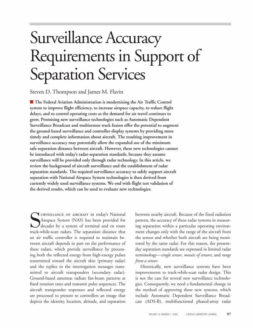
Although surveillance is an important factor in estab-lishing separation standards, it is not the only factor, as illustrated in Figure 1. Consequently, any safety analy-sis comparing the separation measurement accuracy of different surveillance systems must constrain the other factors affecting separation. For example, an analysis of a theoretically perfect surveillance system that mod-els only surveillance accuracy against a target level of

RadarRadarRadarRadar

Microwavetower

Microwavetower

ControllerController

Communicationlatency

Surveillanceaccuracy

Relativegeometry

Airspeed

FIGURE 1. Role of surveillance in separation standards. Surveillance provided by radar and aircraft transponders are only one component of the separation process. Aircraft geometries, airspeed, and communications command and control latency also contribute significantly.



safety would indicate that existing separation stan-dards could be reduced substantially. But this indica-tion would not be supported by other elements that contribute to how far aircraft can move toward each other and be safely separated. The factors illustrated in Figure 1 include time (command and control latency) and relative velocity (airspeed and relative geometry).

The command and control loop between the con-trollers and the aircraft also affects separation speci-fications. Air traffic controllers provide the required separation by issuing clearances, including routings, vectors (headings), and altitude assignments, accom-plished through a very high frequency (VHF) voice channel, with a common channel being assigned to a given airspace. Communications between the control-ler and pilots is subject to interference when more than one person attempts to speak at the same time. There is also opportunity for misunderstanding because of less than perfect reception or because of human error.

Airspeed is an obvious element affecting separation standards. Aircraft in the terminal area where three-mile separation is maintained are normally limited to 250 knots indicated airspeed, while aircraft in the en route environment may have ground speeds over 600 knots.

The relative geometry of the aircraft depends on the air traffic operations such as the traffic-flow pat-terns. For instance, it is clearly easier for a controller to provide separation to an incoming stream of arriving traffic in trail at the same airspeed, but more difficult to provide separation to crossing traffic or traffic that is climbing or descending relative to other traffic. Our approach is to determine the Required Surveillance Performance accuracy for the separation standards in the existing environment in which all of the other contributions remain constant.

Required surveillance accuracy and Error analysis

The FAA has a goal expressed in its Operational Evo-lution Plan [7] and FAA Flight Plan [8] to increase ca-pacity and reduce constraints in the NAS. One area that would provide benefits is increasing the airspace in which three-mile separation is allowed. Partly on the basis of a Lincoln Laboratory analysis of the per-formance of newer monopulse secondary systems [4],

the FAA has recently issued approval to extend the range from a single-site sensor for which three-mile separation is allowed from forty miles to sixty miles for Airport Surveillance Radar 9 (ASR-9) with monopulse sensors. This extension was implemented by a change to FAA Order 7110.65. An extension past sixty miles would have required a software change, since current FAA terminal systems do not report targets beyond sixty miles.

A natural extension to this approach is to define the Required Surveillance Performance accuracy require-ments for which any technology can be used to pro-vide the currently approved three-mile and five-mile separation. This Required Surveillance Performance is based on existing legacy systems for which three-mile and five-mile separation is provided but will al-low surveillance systems based on new technologies other than radar to prove that they can provide accept-able service. This relaxation of requirements offers the potential of further increasing the airspace in which three-mile separation and, in some specific cases, five-mile separation are approved by using alternative sur-veillance techniques such as ADS-B in airspace where radar coverage is unavailable.

In addition, an unambiguous standard, indepen-dent of a given technology, will facilitate potentially new surveillance applications such as multisensor track fusion. As new technologies are introduced and improvements to existing technologies are made, a Re-quired Surveillance Performance based on service per-formance and not on a given sensor type could become a consistent standard by which innovative technologies and techniques can be compared and approved for use in the NAS. The separation standards need not be up-dated with each additional sensor improvement.

A recent precedent to this approach was taken in the field of navigation. The navigation performance requirements historically have been based on fielded equipment such as the VHF Omnidirectional Range (VOR) for en route navigation and the Instrument Landing System (ILS) for precision landing guidance. Now, the Required Navigation Performance sets re-quirements for services and allows any new technolo-gy to provide that service if it meets the requirements, which has permitted new navigation technologies such as GPS to be used in the NAS.



Required Surveillance Performance Accuracy Metric

The Required Surveillance Performance accuracy met-ric refers to the standard of measurement performance that must be met to support the separation services provided by air traffic control. One obvious surveil-lance accuracy metric is the accuracy of the sensor in making target position measurements. There are two problems with using position accuracy as the primary metric for Required Surveillance Performance. One is that air traffic control provides a separation service rather than a positioning service. The other is that er-rors in measured separation depend on whether the same or independent sensors are providing the posi-tion estimates. The use of independent sensors with the same position-measurement errors will result in relatively larger errors in measured separation. If the Required Surveillance Performance is based solely on position-measurement accuracy and set to allow the use of independent sensors, then currently acceptable single-sensor performance will not meet the standard.

The approach taken in this analysis is to quantify the Required Surveillance Performance both in terms of limits on errors in measuring target separation dis-played to the controller and on geographical position accuracy. This approach allows a direct comparison between single-sensor surveillance and cases involving independent sensors or surveillance systems.

The Required Surveillance Performance accuracy derived in this analysis uses errors in displayed separa-tion as the primary accuracy metric and expresses the requirement as limits on the probability distribution of the errors. Because controllers provide radar vectors to fixes and airports and are responsible for obstacle avoidance, the Required Surveillance Performance also includes a geographical accuracy requirement.

Reporting and Error Characteristics of Surveillance Sys-tems That Include Primary Radar

At most terminal and en route facilities a primary radar is collocated with the beacon sensor. Both sen-sors independently make position estimates of targets. When the software determines that those position estimates are for the same aircraft, the target reports are declared a merged target and the position report is characterized as reinforced. In the event a target is not

reinforced it may be beacon only, meaning the prima-ry did not report a target in a near enough position to reinforce the beacon report, or it may be characterized as search only, meaning the primary reported target was not reinforced with a beacon report. The position estimate is reported as range (r) and angle (q) from the sensor location. Beacon-only and search-only re-ports contain the r-q measurement from the respec-tive sensor. For merged targets the position estimate of only one of the sensors is reported.

Modern primary radars employ narrowband Dop-pler filtering and distributed processing to improve target detection and position accuracy and to lower false-alarm rates. In good weather and in the absence of clutter, the performance of modern radars in mea-suring aircraft position is better than that of a sliding-window beacon sensor, but not as good as a mono-pulse beacon sensor.

In the presence of weather, ground, and airborne clutter (e.g., birds), the performance of a primary ra-dar will degrade; in the worst cases it will not be able to reinforce a target that is being declared by the collo-cated beacon sensor. For that reason, the sliding-win-dow beacon performance is considered the baseline for acceptable performance.

Error Characteristics of Secondary Radar Sensors

Secondary radar error characteristics include errors in estimating range and azimuth to the target. Range er-rors are due primarily to errors in measuring the inter-val between the instant an interrogation is sent from the radar and the time a reply is received from the aircraft’s transponder, including errors in the accuracy with which the sensor can measure the time interval and variations in the allowed turnaround time of the transponder. Range errors due to timing are relatively small (typically less than two hundred feet) and do not increase with range. Refraction effects are significant only at very long range and are excluded in this analy-sis. For the same reason, propagation anomalies such as atmospheric ducting are also not included in this analysis.

Azimuth Characteristics of Secondary Radar Sensors

Azimuth-measurement errors are primarily due to er-rors in estimating the target position within the beam-



width of the transmitted pulse. These errors depend on the technique used to estimate the target’s position within the beamwidth. The older sliding-window AT-CRBS and newer MSSR surveillance sensors use dif-ferent techniques to make azimuth measurements.

Figure 2(a) shows the sliding-window technique, which requires detection of replies in the leading and trailing edges of the beam, where the signal is weak-est. The azimuth of the target is estimated as the cen-ter of the reply train. FAA Beacon Interrogator BI-4 and BI-5 sensors use the sliding-window technique. This technique is susceptible to azimuth inaccuracies or even target splits resulting from missing beacon replies. Interference from other interrogators or tran-sponders can garble signals and cause missing replies. The performance also depends on whether the aircraft has a single transponder antenna on the bottom of the aircraft or two antennas, one on the top and one on the bottom of the aircraft. An aircraft with a single bottom-mounted antenna may miss interrogations or have its reply blocked during a turn when the bottom of the aircraft is pointed away from the sensor.

Newer MSSR sensors use multiple beam patterns for interrogations that allow an azimuth measure-ment from a single transponder reply, as shown in Figure 2(b). FAA Mode S and BI-6 sensors use this monopulse technique to attain a three-fold improve-ment in measuring azimuth. A detailed description of these two azimuth estimation techniques is given by

V.A. Orlando [9]. M.C. Stevens’s textbook provides an excellent description of secondary surveillance systems [10].

Errors in Measured Separation from Independent Surveillance Systems

The error in measured separation between two aircraft depends on whether the position of the two targets is reported by the same or independent surveillance sen-sors. Two factors add to the errors in the measured separation error displayed to a controller when inde-pendent sensors are reporting the aircraft positions; uncorrelated position-measurement errors and differ-ences in track update.

Surveillance systems will generally have bias errors associated with their position estimates. When the same sensor is used to measure the position of both targets, bias errors in position estimates associated with that sensor are not reflected in the separation measure-ment.

When a controller is separating two aircraft by using the estimated positions on a display, the tar-gets are updated at different times. This time differ-ential introduces an error in the displayed separation because of the motion of one aircraft relative to the other between updates. With a single sensor, for two target aircraft relatively near each other, the time be-tween updates can be explicitly computed and is gen-erally small. However, in the case of independent sen-

ATCRBSreplies

Trailing-edgedetection

Antenna Leading-edgedetection

Aircraftazimuth

measurement

Antenna

Aircraftazimuth

measurement

∆

ΣBoresight

θ

FIGURE 2. Azimuth estimation with secondary radar; (a) the sliding-window beacon interrogator and the Air Traffic Control Ra-dar Beacon System (ATCRBS) replies; (b) the Monopulse Secondary Surveillance Radar (MSSR). The control pattern used for sidelobe suppression is omitted for clarity. Σ and ∆ indicate the center lobe and side lobe of the MSSR, respectively. q, the azi-muthal angle deviation from the center, is calculated from the relative intensities of the center lobe and side lobe signals. These figures are reproduced from V.A. Orlando’s article in the Lincoln Laboratory Journal [9].

(a) (b)



sor systems, the target updates are asynchronous and the time difference between target updates is generally larger, depending on the update rates of the indepen-dent sensors. The asynchronous nature of indepen-dent sensor systems can result in increased errors in displayed separation.

monte Carlo analysis of sensor Errors

We modeled sensor errors and performed a Monte Carlo analysis by using the methods described in Thompson and Bussolari [5]. Tables 1 and 2 list the radar source errors that are used in the analysis. The error values listed in the tables are based on radar specifications and field data from ARCON Corpora-tion for radars in the Southern California Terminal Radar Approach Control (TRACON) [11], and from Lincoln Laboratory for radars in the Northeast [12].

The errors for individual radars are in good agreement with the errors for radars reported in a study conduct-ed by Lockheed Martin and included as an appendix in the ARCON report. The scan time of the antenna determines the length of time between target updates. While the position estimates are not affected, the mo-tion of the targets between their respective updates re-sults in errors in displayed separation.

Table 3 summarizes the cases analyzed and com-pares the Required Surveillance Performance and the current technology model. The Required Surveillance Performance system modeled for three-mile separa-tion was the short-range ATCRBS sliding-window sensor collocated with a primary radar. The primary-radar position reports are normally used in providing three-mile separation to aircraft, but the beacon-sen-sor reports are used and are acceptable when primary

1 MSSR (Monopulse Secondary Surveillance Radar) can process both Mode Select Beacon Systems (Mode-S) and Air Traffic Control Radar Beacon System (ATCRBS) transponders in a monopulse fashion.

2 The Azimuth Change Pulse (ACP) is 1/4096 of a scan.3 A three-mile separation between aircraft is assumed in this trial at 200 kts.

Table 1. Sensor Error Sources Used in Monte Carlo Simulations for Beacon Sensors

MSSR1 ATCRBS sliding window Short range Long range Short range Long range

Registration errors Location bias 200 ft (0.033 mi) uniform in any direction s = 115 ft (0.019 mi)

Azimuth bias ± 0.3° uniform s = 0.173°

Range errors Radar bias ± 30 ft (0.005 mi) uniform s = 17 ft (0.003 mi)

Radar jitter 25 ft RMS s = 25 ft (0.004 mi)

Azimuth errors Azimuth jitter s = 0.068° (0.8 ACP2) s = 0.230° (2.6 ACP2)

Data dissemination Range 1/64 mi 1/16 mi 1/64 mi 1/16 mi quantization Common s = 27 ft s = 110 ft s = 27 ft s = 110 ft Digitizer 2 format (0.005 mi) (0.018 mi) (0.005 mi) (0.018 mi)

Azimuth 360° 360° 360° 360° (4096 pulses) (4096 pulses) (4096 pulses) (4096 pulses) s = 0.025° s = 0.025° s = 0.025° s = 0.025°

Scan-time 4–5 sec 10–12 sec 4–5 sec 10–12 sec uncorrelated errors3 s = 219 ft s = 536 ft s = 219 ft s = 536 ft (0.036 mi) (0.088 mi) (0.036 mi) (0.088 mi)



Table 2. Transponder Error Sources Used in Monte Carlo Simulations for Beacon Sensors

Mode S ATCRBS

Range errors ± 125 ft (0.021 mi) uniform ± 250 ft (0.041 mi) uniform s = 72 ft (0.012 mi) s = 144 ft (0.024 mi)

Table 3. Summary of Cases Analyzed for Three-Mile and Five-Mile Separation Required Surveillance Performance Accuracy

Required surveillance Current technology performance representative model

Three-mile separation

Radar type Short-range primary Short-range collocated with MSSR sliding window

Range (nautical miles) 40 60

Display system None None processing

Aircraft speed 250 kts 250 kts and geometry 3 mi in trail 3 mi in trail

Sensor Single site Single site configuration

Five-mile separation

Radar type Long-range Long-range sliding window MSSR

Range (nautical miles) 200 200

Display system HOST1 processing HOST1 processing processing

Aircraft speed 600 kts 600 kts and geometry 5 mi in trail 5 mi in trail

Sensor Single site Single site configuration

performance degrades with interference or clutter. Thus it is the performance of the short-range sliding-window beacon sensor that is used to establish the un-conditionally acceptable performance. The aircraft are assumed to travel at 250 knots (the speed limit in the terminal area) up to a range of forty miles from the sensor. It was assumed that there was no DSP and that

the reports went directly from the sensor to the con-troller’s display. The representative case for new sys-tems is the MSSR system, approved for use to a range of sixty miles.

The Required Surveillance Performance model in widespread use for five-mile separation was chosen to be the long-range ATCRBS sliding-window beacon

1 HOST is the NAS automation host computer.



3 miles in trail

Range tomidpoint

40 to 60 miles

φ

at 250 kts

FIGURE 3. Relative geometry for three-mile separation cases with a single beacon sensor tracking both aircraft. Updates are at five-second intervals. Here, f is the orientation of the aircraft in trail relative to the radar beacon.

5 miles in trailat 600 kts

Range tomidpoint200 miles

φ

FIGURE 4. Relative geometry for five-mile separation cases with the aircraft tracking by a single beacon sensor or two in-dependent beacon sensors tracking the aircraft. Updates are at twelve-second intervals. Here, f is the orientation of the aircraft in trail relative to the radar beacon.

sensor at a range of 200 miles, separating aircraft with a ground speed of 600 knots. These systems are nor-mally operated in a mosaic environment. At the sort-box boundaries between radar coverage areas there is normally stitching and hopping of targets as they cross from a sort box that has one radar assigned as primary sensor to another sort box that has a different assigned radar. For the purposes of this analysis, it is assumed that it is conditionally acceptable for five-mile separa-tion to use two different radars tracking the aircraft only as they cross sort-box boundary lines. This level of performance was not considered acceptable across all en route airspace. An MSSR long-range system is assumed for the new technology case.

Three-Mile Separation. The procedure followed for the three-mile separation cases was to determine the distribution of errors in measured separation observed, on average, for two aircraft that were three miles apart in trail, as illustrated in Figure 3. Aircraft speed was chosen to be 250 knots (speed limit in the terminal area), as listed in Table 3. The aircraft were random-ly oriented relative to the radar by randomly choos-ing an angle f, as illustrated in Figure 3, for each trial. The Monte Carlo simulations using the beacon error characteristics described in Table 2 were run for each of the cases listed in Table 3. Both the sliding-window beacon sensor and the collocated primary radar are listed for the Required Surveillance Performance case in Table 3 although, as described above, the sliding-window beacon performance is considered the base-line acceptable performance.

Five-Mile Separation. The procedure followed for the five-mile en route case was to model two aircraft five miles in trail traveling at a 600 knot ground speed and tracked by sensors, as described in Table 3 and shown in Figure 4. The Required Surveillance Perfor-mance case was modeled as a single long-range sliding-window sensor. The new technology case was modeled as a long-range MSSR sensor. The midpoint of the separation of the aircraft was kept at a constant range of two hundred miles, as described in Table 2.

Simulation Trials Results

The results of the one million trials for the Required Surveillance Performance case listed in Table 3 for three-mile separation are presented in Figure 5, which

illustrates the errors in measured separation as a func-tion of range. The highlighted distance slice is at forty miles, which corresponds to the results shown in Fig-ure 6(a)—the distribution of sensor measured sepa-rations for aircraft that are actually three miles apart. The jaggedness in the distributions is due to the dis-



crete allowed position reports of the Common Digi-tizer 2 (CD2) format and the even distribution of the bin sizes in the histogram.

There are a finite number of allowed separations and, regardless of the size of the bins, the allowed re-ports will fall into one bin or another. If the number of trials is doubled, the graphs will look identical. If the histogram bin size is changed, then a different ragged-ness pattern will appear. The corresponding results of the one million trials for the tests represented in Table 3 for three-mile and five-mile separation are presented in Figures 6 and 7. Note that these are sensor error distributions and do not yet include the DSP errors that apply to the five-mile separation cases, as listed in Table 3.

Display System Processing Errors

DSP errors are included in the Required Surveillance Performance accuracy for the five-mile separation cases listed in Table 3. The three-mile separation cases rep-resentative of terminal operations were assumed direct

to glass—presented to the operator’s screen without any analysis. This is a conservative assumption, since many terminals use one of several available DSP sys-tems.

DSP errors are introduced by the system between the sensor reports and the separation displayed to the controller on the screen. The differences between sep-aration as measured by sensor reports and separation displayed to the controller may result from display latencies, coordinate transformation, asynchronous updates, and missed updates or tracking errors. The DSP errors depend on the system design and automa-tion software, as well as whether the aircraft are be-ing tracked by the same radar or different radars. The NAS automation host computer (HOST) system in the Air Route Traffic Control Centers (ARTCC) was chosen as representative because it is in widespread use and because it is commonly used at ARTCCs and is acceptable for five-mile separation.

DSP errors were measured from data rather than modeled. This measurement was accomplished by

Pro

bab

ilty

den

sity

0.00

0.02

0.06

0.03

0.04

0.05

0.01

3.02.52.01.5

4.54.03.5 0

Separation (mi)

Range

(mi)

50

100

FIGURE 5. Probability density of measured separation as a function of range for an ATCRBS sliding-window short-range sensor and two aircraft separated by three miles. The blue slice shows the measured separation of two aircraft at 40 mi distance.



1.5 2.0 2.5 3.0 3.5 4.0 4.50

1

2

3

4

5

6

7

8

Estimated separation (mi)

= 3.0010 miσ = 0.0799 mi

Actual separation = 3.0 mi

µ

1.5 2.0 2.5 3.0 3.5 4.0 4.50

1

2

3

4

5

6

7

8


Num

ber o

f sa

mpl

es ×

104 (

106 t

otal

tria

ls)

Num

ber o

f sa

mpl

es ×

104 (

106 t

otal

tria

ls)

= 3.0040 miσ = 0.1641 mi


µ

Range 40 mi Range 60 mi

FIGURE 6. Results of Monte Carlo simulation in measured separation error for three-mile separation (aircraft velocities 250 knots): (a) single ATCRBS sliding window long-range radar; and (b) single MSSR short-range radar. Here, m is the mean value of the data and s is the standard deviation.

FIGURE 7. Results of Monte Carlo simulation in measured separation error for 5-mile separation (aircraft velocities 600 knots): (a) single ATCRBS sliding window long-range radar; and (b) single MSSR long-range radar. Here, m is the mean value of the data and s is the standard deviation.

(a) (b)

0 2 4 6 8 100

0.5

1.0

1.5

2.0

2.5

3.0

3.5

4.0


Num

ber o

f sa

mpl

es ×

104 (

106 t

otal

tria

ls)

= 5.0647 miσ = 0.8018 mi


µ

0 2 4 6 8 100

0.5

1.0

1.5

2.0

2.5

3.0

3.5

4.0


Num

ber o

f sa

mpl

es ×

104 (

106 t

otal

tria

ls)

= 5.0061 miσ = 0.2553 mi


µ

Range 200 mi Range 200 mi

(a) (b)

comparing the separation of targets on the basis of sensor reports received at the Boston ARTCC to the separation of the same targets on the controller’s dis-play. The data reported by the sensors are recorded as U.S. Air Force’s Radar Evaluation Squadron (RADES) format data as it enters the facility. The position re-ports are recorded in latitude and longitude and are

based on the r-q reports of the individual sensors. All reports of sensors tracking targets are recorded; con-sequently, there are multiple reports for each aircraft being tracked.

The separation displayed to the controller is com-puted from the position reports, as recorded on the sys-tem analysis report (SAR) tapes. The position reports



4.93 4.94 4.95 4.96 4.97 4.9810

12

14

16

18

20

22

Time × 104 (seconds)

Measured separation (SAR data)Displayed separation (RADES data)

Sep

arat

ion

(mi)

FIGURE 8. Comparison of measured separation (in miles) versus time for the Radar Evaluation Squadron (RADES) data and the system analysis report (SAR) data for a sample case. The differences evident in the figure represent the er-rors introduced by the Display System Processing (DSP).

include the beacon code, the time, and the Cartesian x-y position on the stereographic plane. Each ARTCC displays target positions on a stereographic plane with a point of origin (x = 0, y = 0) and point of tangency (where it touches the earth) defined for that facility’s airspace. All target position reports received from field sensors are projected onto that common plane. The position report from only one sensor is provided to the controller’s display for a given target, and that is the position report recorded in a file on the SAR tape. The SAR data, in a separate file, records which sensor is be-ing utilized for reports for a given target as a function of time. Thus it is possible to determine which sensor’s target data were presented to the controller and the x-y position on the stereographic plane that was used to present the target position. The time between the SAR recording and the display is assumed negligible.

To compare the separation reported by the sensors to that displayed to the controllers, recorded RADES data and SAR data tapes for a period of 1045–1415 universal time coordinated (UTC) on 6 October 2005 were obtained from the Boston ARTCC. The RADES data files were sent to Lincoln Laboratory and the cop-ied SAR data tapes were sent to the FAA’s William J. Hughes Technical Center (WJHTC) in Atlantic City, New Jersey.

The RADES data files were examined at Lincoln Laboratory and fifty aircraft pairs were manually se-lected, with criterion that the aircraft pair were in close horizontal proximity over an extended period of time (tens of minutes) and were at the same or nearly the same altitudes. The fifty cases were identified to WJHTC by providing the two beacon codes, the start and stop times, and the approximate latitude and lon-gitude. On the basis of case descriptions, WJHTC then processed the SAR tapes and provided Lincoln Laboratory with the SAR data of the beacon codes of interest, which included two files for each case. One file contained the sensor used as a function of time for each of the two beacon codes and the other con-tained the time, beacon code, x-y position on the ste-reographic plane, and Mode C* reported altitude for each report.

The RADES data files, which contain data for all radars, were filtered to create files that matched the sensors identified by the SAR data as those used for display on the controller’s screen. The separation as a function of time between the targets in the RADES data was computed by converting the RADES-format-ted latitude and longitude reports to the earth-centered earth-fixed (ECEF) reference grid and computing the separation at each update report. This separation was computed each time a beacon target produced a new position report. The separation of the beacon targets as reported in the SAR data was computed directly from the x-y position reports representing position on the stereographic plane, and was also updated with each beacon report.

The computed separation between the two beacon targets as a function of time as recorded by the sen-sors (RADES data) and as presented to the controller (SAR data) was compared. Figure 8 shows an example of a plot comparing the RADES and SAR data. The difference between the two reported separations as a function of time was measured for each update to pro-vide a histogram of the differences in separation for each case. This measurement represents a probability distribution of the errors introduced by the DSP be-tween what was reported by the sensors and what was displayed to the controllers for a single case of two air-craft being separated for a period of time.

Of the fifty cases chosen, only thirty-nine were able

* Mode C is the transponder reply mode that includes altitude and coding.



to be reduced from the SAR data, in part due to mul-tiple aircraft with the same beacon code in the SAR data and in part due to unavailable SAR tapes for the total time of interest. These thirty-nine cases were added together and normalized to take out any bias introduced by the particular selection of cases. The fi-nal results are the distributions of HOST DSP errors presented in Figure 9.

Total System Error

Figure 10 presents the results of numerical convolution of the DSP error with the sliding-window long-range radar error. This analysis was accomplished by adding a randomly sampled sensor error from the sensor er-ror distribution, shown in Figure 7(a), to a randomly sampled DSP error from the DSP error distribution, shown in Figure 9. One million random samples were taken from each distribution and added together to create the data shown in Figure 10. This result repre-sents the total system error for the five-mile separation Required Surveillance Performance case.

flight test validation

The purpose of the flight test was to validate the mod-eled error sources of the sensors used in the analysis by comparing true separation, as provided by position recordings from GPS on board two aircraft, with sen-sor measured separation, as recorded from sensors at Boston ARTCC. This test was accomplished by flying

two aircraft approximately three miles apart in trail over a large portion of Boston Center airspace. The flight path was designed to provide data from approxi-mately ten sensors, including long-range and short-range sliding-window and MSSR beacon sensors. The use of two aircraft allowed a comparison of measured separation with true separation rather than measur-ing the accuracy of the position report of the aircraft. Measured separation error is the primary metric used in the analysis.

Data Recording

The flight test validation made use of Lincoln Lab-oratory’s Falcon 20 and Gulfstream G2 jet aircraft. The Falcon 20 is shown in Figure 11, and the G2 is shown in Figure 12. Each of the test aircraft carried a GPS/laptop recording system and operator, and was equipped with a GPS antenna.

The airborne data recording portion of the flight test validation recorded WGS-84 ECEF reference po-sition data from two GPS receivers, one in each air-craft. An Ashtech Model GG24 GPS plus GLONASS sensor was used in both aircraft. The GG surveyor provides position accuracy on the order of seven to twenty meters, and updates positions once per second [13]. This position information was sent to a laptop via a serial port connection. GPSLog, a custom-writ-ten program, wrote the updated reports to a file on disk. GPSLog utilizes a 9600 baud 8N1 serial com-

–4 –3 –2 –1 0 1 2 430

2

4

6

8

10

12

Difference in separation for SAR and RADES data (miles)

Num

ber o

f oc

curr

ence

s ×

104

FIGURE 9. Histogram of NAS automation host computer (HOST) DSP errors for a single sensor measured from thir-ty-nine sample cases of aircraft pairs recorded at Boston Air Route Traffic Control Centers (ARTCC) on 6 October 2004.

0 1 3 5 7 92 4 6 1080

1.0

0.5

1.5

Estimated separation (miles)

Num

ber o

f sa

mpl

es ×

104

(106 t

otal

tria

ls)

FIGURE 10. Total system error for long-range sliding-window sensor at two-hundred-mile range with single-sensor HOST system display processing.



FIGURE 11. Falcon 20 lead aircraft in flight test. FIGURE 12. Gulfstream G2 trailing aircraft in flight test.

munication format to communicate with the GG sur-veyor. The software uses a one-second timer to poll the GPS for its current position, allowing for a more robust connection. If the GPS fails to reply to a poll in a timely fashion, the operator is notified and can begin troubleshooting. Additionally, the GG surveyor has the capability of recording position updates to in-ternal memory for later offline retrieval, providing a backup of the data recording.

After completion of the flight test validation, the recorded GPS data were post-processed to obtain time-stamped ECEF position reports in a form that could be read into MATLAB. All analysis was done in MATLAB. GPS time does not incorporate the leap-seconds used in UTC time, and the current offset be-tween GPS and UTC time is thirteen seconds. This difference was subtracted and the data analyzed was in UTC time.

The ground data recording portion of the flight test validation consisted of two separate systems. The sen-sor data consisted of a recording of all the CD2 for-mat messages from the fourteen radars in the USAF RADES format. Nine different sensors actually tracked the two test aircraft for significant time dur-ing the flight. The data view screen lists a row for each report of each sensor color coded by message type; red for beacon only, green for search (primary only), and blue for reinforced. The data can also be filtered by sensor(s) and beacon codes.

The RADES software was used to extract, time, r, q, latitude, longitude, and altitude for both test air-craft from all sensors that tracked the two test aircraft.

These data files were converted to a format that could be read into MATLAB.

The data displayed to the controller was recorded on SAR tapes. These tapes are produced by software running on the HOST computer, and they record all of the display updates sent to the Display System Re-placement screen. These tapes were sent to WJHTC in Atlantic City, New Jersey, for post-processing. The product of this processing was a file containing time, aircraft ID, radar ID, x-y position on the stereographic plane, and altitude for the test aircraft. The SAR data contain only the data from the sensor that was used to display the target on the controller’s screen. This file was then read into MATLAB for further process-ing and comparison of the displayed separation to the measured separation as well as the GPS truth data. Figure 13 illustrates the relationship between the vari-ous airborne and ground data recordings. An excellent treatment of the various coordinate systems and how to transfer between them is contained in P. Misra and P. Enge [14].

Flight Test Results

Radar reports from the sensors were recorded as they were received at Boston Center (RADES) and as pre-sented to the controllers’ display (SAR). The RADES data files were filtered for the two beacon codes of the flight test aircraft. Figure 14(a) is a plot of the radar data showing all reports for both test aircraft by all ra-dars. The aircraft were tracked by nine different sen-sors in Boston Center’s airspace during the flight test.

The GPS position data recorded on board the flight



Air route traffic control center

Sensor data Displayed data

Measured separation

Derived required surveillance performance

Displayed separation

Latitude, longitudereference system

Data used to validateMonte Carlo simulationresults

Data derived fromany observed aircraftpairs

Reference data

True separation

x, y stereographicplane reference system

Earth centered, earth fixedx,y,z reference system

30

–30

0

60

–60

75

–180–220 –120 –60 –40

CommonDigitizerformat disc

SystemAnalysisReport

FAA Tech Centerdata extractionsoftware

USAFRadar Evaluation Squadronsoftware

Controller displays

Displaysystem

replacement

Radars

z

x y

Twoaircraft

GPSreceiver

GPSreceiver

Aircraft 1

(x1−x

2)

2 + (y1−y

2)

2 + (z1−z

2)

2

Aircraft 2

Compare

True

Point oftangency

x

yCenter of mass

Referencemeridian

Compare

Sensor measument errors Display processing errors

Convolve

Time (sec)

A/C

sep

arat

ion

(nm

i)

0

2.5

3.5

4.0

3.0

50 100 150 200Time (sec)

A/C

Sep

arat

ion

(nm

i)

A/CSeparation

(nmi)

0

2.5

3.5

4.0

3.0

50 100 150 200Time (sec)

A/C

Sep

arat

ion

(nm

i)

0

2.5

3.5

4

3

50 100 150 200

Displayed separation error

Hostcomputer

Measured Displayed

00:29:59.745

00:29:59.745

00:29:59.725

00:29:59.730

00:29:59.765

00:29:59.765

00:29:59.780

00:29:59.800

00:29:59.810

00:29:59.810

00:29:59.810

00:29:59.830

00:29:59.785

00:29:59.800

00:29:59.805

00:29:59.820

322.910

322.031

0.967

290.918

228.428

233.086

233.965

211.465

58.711

210.322

218.145

237.305

157.236

318.604

319.219

317.109

41 13 30.552 N

41 46 38.402 N

41 43 49.931 N

47 39 49.931 N

39 4601.926 N

40 14 46.243 N

40 34 04.708 N

40 57 38.461 N

43 55 04.574 N

40 48 27.464 N

41 13 29.037 N

41 04 35.745 N

42 27 22.614 N

42 00 10.152 N

42 46 46.255 N

41 43 49.914 N

076 21 53.057 W

077 00 28.917 W

071 35 53.411 W

071 08 10.606 W

073 17 55.456 W

073 05 26.013 W

072 38 40.731 W

074 31 58.217 W

069 34 10.505 W

074 37 49.761 W

074 22 54.823 W

079 44 11.115 W

077 32 59.210W

077 47 33.517 W

078 28 25.520 W

077 20 49.921 W

Time AzDegs Lat Lon

t x y z00:29:59.745

00:29:59.745

00:29:59.725

00:29:59.730

00:29:59.765

00:29:59.765

00:29:59.780

00:29:59.800

00:29:59.810

00:29:59.810

00:29:59.810

00:29:59.830

00:29:59.785

00:29:59.800

00:29:59.805

00:29:59.820

322.910

322.031

0.967

290.918

228.428

233.086

233.965

211.465

58.711

210.322

218.145

237.305

157.236

318.604

319.219

317.109

41 13 30.552 N

41 46 38.402 N

41 43 49.931 N

47 39 49.931 N

39 4601.926 N

40 14 46.243 N

40 34 04.708 N

40 57 38.461 N

43 55 04.574 N

40 48 27.464 N

41 13 29.037 N

41 04 35.745 N

42 27 22.614 N

42 00 10.152 N

42 46 46.255 N

41 43 49.914 N

076 21 53.057 W

077 00 28.917 W

071 35 53.411 W

071 08 10.606 W

073 17 55.456 W

073 05 26.013 W

072 38 40.731 W

074 31 58.217 W

069 34 10.505 W

074 37 49.761 W

074 22 54.823 W

079 44 11.115 W

077 32 59.210W

077 47 33.517 W

078 28 25.520 W

077 20 49.921 W

Time AzDegs Lat Lon

t x y z

One sensor per aircraftAll sensors for all aircraft

t AC SENSOR ρ θ LAT LONG ALT t AC SENSOR x y ALT

RADESsoftware

FAATCsoftware

CDformatdata

SARdata

FIGURE 13. Airborne and ground data recording during the flight test. The true separation is derived from the Global Position-ing System (GPS) reference data of the two aircraft. The measured separation is derived from the ground sensor data as it en-ters the facility. The displayed data are recorded in SAR format.

using the Mode C reported altitudes of the aircraft. Computations showed that the 100 ft resolution in the Mode C altitude reports contributed insignificant errors. The GPS separation was considered truth in the remainder of the analysis and used to measure the errors in the RADES and SAR data in separation mea-surement. Figure 15 shows the aircraft separation dur-ing the flight test.

The sensor azimuth-measurement errors result in position and separation measurement errors that in-crease with range from the sensor. To compare the flight test data with the error model it is necessary to compute the range from each sensor as a function of time. The aircraft GPS position data were used to compute the range to the midpoint of the two aircraft from each of the radars. Figure 16 depicts a sample plot of the horizontal range from the midpoint of the two aircraft to the Coventry (COV) radar.

test aircraft consisted of WGS-84 ECEF x-y-z posi-tions of the aircraft updated every second. The GPS time was corrected to UTC time by subtracting thir-teen leap-seconds from the recorded GPS time. The ECEF flight progress strip position data were convert-ed to latitude and longitude for comparison with the radar data. Figure 14(b) is a plot of the position re-ports as recorded by the GPS units. Flight test aircraft safety procedures required that the data recording be off during take-off and landing, as seen by gaps in the tracks at the beginning and end of the flight test when compared to the radar observations shown in Figure 14(a).

The GPS position data were used to compute the three-dimensional separation of the aircraft. The one-second update data from the two GPS units were in-terpolated to common times. The three-dimensional separation was converted to horizontal separation by



(a)

FIGURE 14. Flight test data for the Falcon 20 and Gulfstream G2: (a) flight racks from radar data (RADES) and location of sen-sors; (b) GPS recorded position of the flight test aircraft. The Falcon 20 is depicted in red, and the Gulfstream G2 is in blue. Sensor locations, specifically QHA, Hartford, are not necessarily located in the named towns. The five sensors not shown in the figure are QEA, North Truro, Massachusetts (ARSR/BI5); QXU, Remson, New York (ARSR/BI5); QHB, St. Albans, Vermont (FPS67B/Mode S); QRC, Benton, Pennsylvania (FPS67B/BI5); and QIE, Gibbsboro, New Jersey (ARSR/BI5).

QHA

BDL

COV

QVH

The RADES data were examined to determine pe-riods of time during the flight test when each sensor was tracking both aircraft with continuous updates. This determination was made by plotting the delta up-date times for both aircraft as a function of time and noting periods in which there were no points above

the normal update rate. The position measurements for both aircraft for the periods of continuous cover-age were then determined for each sensor.

The position measurement of the two flight test aircraft were used to compute the separation measure-ment of the sensor as a function of time. The sensor-

(a) (b)

0 500 1000 1500 2000 2500 3000 3500 40000

5

10

15

20

25

Time (sec)

Hor

izon

tal s

epar

atio

n (m

i)

Takeoff

Flight testbegins

Flight testends

Flyout

FIGURE 15. GPS recorded position of the flight test aircraft. The figure on the right is an expanded view of the figure on the left, covering the flight test period from 1000 to 2500 seconds.

1000 1500 2000 25002.8

2.9

3.0

3.1

3.2

3.3

3.4

3.5

3.6

3.7

Time (sec)

Hor

izon

tal s

epar

atio

n (m

i)



report update of one of the aircraft. The two aircraft are updated within a short time period, but there is a brief gap between individual airplane updates. An algorithm was developed to determine the separation measurement immediately after the second aircraft update. With the Hartford (QHA) radar as an exam-ple, the red plus signs in Figure 17 illustrate the times

reported r, q, and the aircraft-reported Mode C alti-tude were converted to a local Cartesian coordinate system, and the horizontal separation was computed for the aircraft as a function of time. Although the ac-tual separation of the aircraft is a continuous function of time, the measured separation is a discrete function with each change in the value indicative of a radar

0 500 1000 1500 2000 2500 3000 3500 40000

10

20

30

40

50

60

70

80

90

100

Time (seconds)

Ran

ge (m

i)

FIGURE 16. Range from the Coventry (COV) radar site to the midpoint between the two flight test aircraft as a function of time.

2620 2660 2700 2740 2780 28201.5

2.0

2.5

3.0

3.5

4.0

4.5

Time (seconds)

Ho

rizo

nta

l sep

arat

ion

(m

i)

FIGURE 17. Sampled measurements of the separation of the aircraft by Hartford (QHA) radar. The blue lines represent the displayed separation as a function of time. The red plus signs are the sample separation compared to the GPS-pro-vided true separation. The spikes occur as one aircraft posi-tion is updated prior to the other. The direction of the spikes depends on the order of the updates.

0 20 40 60 80 100 120 140 160 180 200–1.0

–0.8

–0.6

–0.4

–0.2

0

0.2

0.4

0.6

0.8

1.0

Range from sensor to midpoint of two aircraft (nmi)

Mea

sure

d se

para

tion

erro

r (nm

i)

Flight test points in region (predicted by model)

4 (5)

38 (45)

428 (396)

23 (45)

3 (5)

1%10%QHBQHAQRCPVDBDL

FIGURE 18. Modeled error limits versus range for an MSSR sensor. This figure includes reinforced data only. The total number of data points is 496.



0 20 40 60 80 100 120 140 160 180 200

Range from sensor to midpoint of two aircraft (nmi)

Mea

sure

d se

para

tion

erro

r (nm

i)

Flight test points in region (predicted by model)

2 (5)

12 (45)

474 (396)

7 (45)

1 (5)

–3

–2

–1

0

1

2

3

Both aircraft reinforced

One aircraft beacon onlyBoth aircraft beacon only

1%10%QIEQXUQVHQEA

FIGURE 19. Modeled error limits versus range for a sliding-window sensor. The total number of data points is 496.

sampled to compare the measured separation with the true separation. Each point in time represented by a red plus sign indicates a single data point for measured separation by the sensor.

These separation measurements, for each radar, were then compared to the GPS separation that is consid-ered true, and the difference is recorded as a measured separation error. These measurements are plotted as a function of range, based on the range versus time plots computed earlier for each particular sensor. This pro-cedure is used for all radars and is combined on plots designed to show the modeled sensor error limits. Fig-ure 18 shows these data for the MSSR sensor and Fig-ure 19 shows these data for the sliding-window sensor. The numbers in the regions above the 99% error line, below the 1% error line, and between the 90% and 99% error region and between the 1% and 10% er-ror regions are the number of data points measured in these regions and the number predicted by the model. Note the expanded scale for the sliding-window sensor in Figure 19, compared to the MSSR plot in Figure 18. The total number of data points (496) was coin-cidentally the same for both the sliding-window and MSSR sensors.

Sensor Azimuth Performance

The sliding-window sensor performance as measured during the flight test was better than predicted by the error model, while the measured MSSR sensor perfor-mance was more closely predicted by the model. Be-cause the only difference in the model of the MSSR and sliding-window sensors was the modeled azi-muth-jitter errors, a more detailed investigation of the azimuth (q) errors of the sliding-window and MSSR sensors was undertaken.

The RADES data contained the azimuth (qRADES) measurement, based on the antenna position relative to true north for all sensors for both aircraft. The GPS data contained the aircraft position in ECEF coordi-nates, converted to latitude and longitude. Since the location of the sensors was known in latitude and lon-gitude, the bearings from the sensors (qGPS) could be computed by using spherical trigonometry. The total errors in azimuth were defined as qRADES – qGPS, where the GPS measurements were interpolated such that there was a GPS value for each RADES measurement.

The total azimuth errors for both aircraft were plot-ted as a function of time. A curve fit using the low-



FIGURE 20. Azimuth error measurements (qRADES – qGPS) on both flight test aircraft as a function of time for the short-range MSSR sensor at Bradley (BDL): (a) error measurements with polynomial curve fitting and (b) residuals after curve fitting. The three outliers near 350 sec occurred during periods when the track was dropped and reacquired.

0 500 1000 1500 2000 2500 3000–1.0

–0.8

–0.6

–0.4

–0.2

0

0.2

0.4

0.6

0.8

1.0

Time (sec)

Azi

mut

h er

ror (

degr

ees)

4617 G24665 Falcon

0 500 1000 1500 2000 2500 3000–1.0

–0.5

0

0.5

1.0

Time (sec)

Azi

mut

h er

ror (

degr

ees)

(a)

(b)

est-power polynomial that removed any bias from the residuals was used to determine the bias in the mea-surement. Azimuth bias in a sensor can be a slowly varying function of time or a function of the relative bearing from the sensor. The measurement of two test aircraft in trail made it possible to determine that a sensor bias was affecting both aircraft. The residuals about the curve-fitted bias were computed as the azi-muth jitter. These measurements were used to gener-ate a probability distribution of bias and jitter for each

sensor, a process illustrated in Figures 20 and 21 for the short-range MSSR sensor at Bradley (BDL).

The procedure described above was performed for all nine sensors. The standard deviation (s) of the azi-muth (q) jitter error of each sensor is plotted in Figure 22 and compared to the modeled error for the MSSR and sliding-window sensor. Four of the five MSSR sensors performed slightly better than the error mod-el and one slightly worse. Because the performance of the St. Albans sensor (QHB) was close to three of



FIGURE 21. Separation of the azimuth error (q) into azimuth bias and jitter for the Bradley (BDL) short-range MSSR sen-sor.

Bias error

-0.4 -0.2 0 0.2 0.4 0.60

20

40

60

µ = 0.003σ = 0.054

Jitter error

-0.4 -0.2 0 0.2 0.4 0.6

µ = 2.4 × 10–14

σ = 0.050

0

20

40

60

80

Nu

mb

er o

f m

easu

rem

ents

Nu

mb

er o

f m

easu

rem

ents

QEA QIE QVH QXU QHAQHB QRC BDL COV0

0.05

0.10

0.15

0.20

0.25Modeled errorfor sliding windowsensors

Modeled errorfor monopulsesensors

May be inIBI mode

MonopulseSliding window

(deg

)σ

FIGURE 22. Standard deviation (s) of azimuth-jitter errors for the nine sensors recording data for both flight test aircraft; errors for sliding-window sensors compared to MSSR sen-sors. IBI stands for Interim Beacon Interrogator.

the sliding-window sensors, it is not possible to rule out that the sensor may have been in Interim Beacon Interrogator (IBI) mode and acting as a sliding-win-dow sensor. Three of the four sliding-window sensors performed much better than the error model and one performed very close to the model, indicating that there is a relatively wider spectrum of performance in the sliding-window sensor.

All of the measured jitter errors were combined for the five MSSR and four sliding-window sensors and the probability distributions for the respective jitter er-

rors computed. These distributions are shown in Fig-ure 23 for the MSSR sensors and in Figure 24 for the sliding-window sensors.

The cumulative average azimuth-jitter standard de-viation for the MSSR sensors was s = 0.058°, which is in very good agreement with the modeled error source of s = 0.068°. The measurements from five sensors is not statistically significant enough to change the error model, if we keep in mind that the error model is for the least performing system, not the average perfor-mance of all systems.

FIGURE 23. Distribution of azimuth jitter errors for the five MSSR sensors.

σ

–1.5 –1.0 –0.5 0 0.5 1.0 1.5

= 0.15°

Azimuth jitter (deg)

20

0

40

60

80

100

120

140

Nu

mb

er o

f m

easu

rem

ents

FIGURE 24. Distribution of azimuth jitter errors for the four sliding-window sensors.

σ

–1.5 –1.0 –0.5 0 0.5 1.0 1.50

50

100

150

200

250

300

350

= 0.058°

Azimuth jitter (deg)

Nu

mb

er o

f m

easu

rem

ents



The cumulative average azimuth-jitter standard de-viation for the sliding-window sensors was s = 0.15°, which is less than the error model source of s = 0.23°. However, one sliding-window sensor performed very close to the error model, indicating a range of perfor-mance in sliding-window sensors. The error model is designed to model the least performing system of its design, and when there is a relatively wide range of performance, the average performance is statisti-cally better than the lesser performing sensors. The ARCON report [11] notes a similar result in their field measurements of Air Route Surveillance Radar (ARSR) sliding-window beacon sensors in southern California TRACON with a s = 0.119° at a range of greater than sixty miles, although they list a typical modeled error of s = 0.23°.

The difference in the way the sliding-window and MSSR sensors work provides an explanation of why the sliding-window sensor performance has a larger range in performance than the MSSR sensors. MSSR sensors with selective interrogation provide excellent surveillance in heavy traffic environments with high interrogation rates from multiple sensors. Sliding-window sensors perform very well when replies are re-ceived across the beamwidth, typically fifteen to twen-ty hits per beam. However, in dense traffic or a dense interrogator environment, the performance of a slid-ing-window sensor deteriorates. Interrogation efficien-cy decreases when many interrogators are active. This decrease includes other ground-based sliding-window or MSSR sensors as well as airborne interrogations from Traffic Alert and Collision Avoidance (TCAS) radars. The aircraft transponder may be suppressed or actively replying to another interrogation and not reply to a given interrogation from a sensor. In addition, the reply may be garbled if it overlaps with the reply from another transponder. This garbling can cause relatively large errors (on the order of a tenth of a beamwidth, or 0.25°) in azimuth measurements if the missed re-plies are near the edge of the beam. The data from the flight test were taken in a low interrogation environ-ment at a time and altitude where there was not heavy traffic; the higher performance is consistent with the performance of sliding-window sensors in a benign environment. The error model must account for the performance in more challenging environments.

The bias data from all of the sensors were combined to provide a probability distribution of the bias errors, presented in Figure 25. The error model assumed a uniform bias error of ± 0.3°, which has s = 0.173°. The data from the flight test have s = 0.15°, which is in good agreement, although the distribution does not appear to be uniform. This non-uniform distribu-tion would only affect cases using independent sensors when bias errors are not correlated. In the final analy-sis, there were no cases using independent sensors to establish an Required Surveillance Performance. The sensor azimuth-bias-error model will be modified for future analysis.

Measurement of Sensor Report Latencies

The flight test data position measurements were used to analyze the radar report latencies. The time differ-ence between the GPS truth and the SAR data rep-resents the total latency from sensor measurement to display to the controller. The time offset for each sensor was determined by finding the offset (∆ t) that minimized the difference in position measurements between the sensor and GPS data for all measure-ments.

The SAR data errors were calculated by using ECEF x-y-z position reports. For the SAR data, the mathematical approach was to determine the ∆t that minimized the sum of the differences in x, y, and z:

–1.5 –1.0 –0.5 0 0.5 1.0 1.5

Azimuth bias (deg)

50

100

150

200

250

300

350

400

= 0.15°σ

Nu

mb

er o

f m

easu

rem

ents

FIGURE 25. Distribution of azimuth bias errors for all sen-sors.



∆ ∆ ∆ ∆t x y zii i i= + +∑min .

(1)

Figure 26 illustrates a time-offset computation for the SAR data, while Figure 27 illustrates the relationship between ∆ t and ∆xi . The ∆ t was varied until the sum of all ∆xi , ∆yi , and ∆zi for both aircraft was mini-mized.

Four sensors tracked the test aircraft that were dis-played to the controllers and recorded on the SAR data. The latency measurements ranged from 1.2 sec-onds to 2.5 seconds with an average of 1.7 seconds.

selection of Required surveillance performance

Required Surveillance Performance consists of many attributes, including accuracy, latency, update rates, capacity, availability, probability of detection, and con-tinuity. The focus of this analysis was on surveillance accuracy required to support three-mile and five-mile separation. The accuracy requirements were derived from Monte Carlo simulations of modeled legacy sen-sor errors and validated with flight test data. Accuracy in measured separation was the metric chosen. How-ever, geographical position accuracy is also available from the simulation and included as an additional at-tribute.

The Required Surveillance Performance accuracy requirement was derived from the unconditionally

2850 2900 2950 3000 3050 31001.500

1.505

1.510

1.515

1.520

1.525

Time (sec)

ECEF

x-p

ositi

on ×

106 (

m)

GPS positionOriginal recorded SARRecorded SAR with offset

FIGURE 26. Example of SAR versus GPS data used to calcu-late absolute latency. The data were collected from the North Truro radar tracking the Falcon aircraft with a time offset of 1.1 sec.

accepted widespread-use cases from Table 3 for three-mile and five-mile separation. The sensor in the three-mile separation case is the short-range primary sensor collocated with a sliding-window beacon sensor at a range of forty miles, tracking two aircraft three miles in trail at 250 knots. The baseline error in measured separation is taken to be that of the beacon sensor. Though the primary sensor is slightly more accurate, it can degrade in clutter environments; in those cases it is the beacon sensor that is used to provide separation. Also, MSSR sensors can be used to provide three-mile separation when they go into the IBI mode, and their performance is that of a sliding-window sensor. The sensor is in a single-site adaptation; that is, the same sensor is providing position information for both air-craft. No DSP errors were included. It was assumed the reports went direct to glass, as is the nominal case for TRACONs.

The five-mile separation case is for a single long-range sliding-window sensor at a range of 200 miles tracking aircraft five miles in trail at 600 knots. The total error in separation was determined by indepen-dently sampling from the sensor error distribution and the experimentally measured HOST DSP error dis-tribution and adding these errors. This is the nominal system in use at ARTCCs today.

∆x2

∆t

∆x1

∆xi

FIGURE 27. Illustration showing the relationship between ∆ t and ∆ x in Equation 1. ∆ t is adjusted to minimize the sum of ∆ x (and ∆ y and ∆ z).



reference system approach based on the specifications of representative sensors. This Required Surveillance Performance is applicable to the extent that a surveil-lance system is similar in performance characteristics to the legacy systems used to derive a baseline.

Table 4. Required Surveillance Accuracy

Accuracy in measured separation Three-mile separation Five-mile separation

Standard deviation No greater than 0.16 mi No greater than 0.8 mi

No more than 10% of the error ± 0.28 mi ± 1.4 mi distribution shall exceed

No more than 1% of the error ± 0.49 mi ± 2.4 mi distribution shall exceed

No more than 0.1% of the error ± 0.65 mi ± 3.3 mi distribution shall exceed

Geographical position accuracy s < 0.20 mi s < 1.0 mi

Latency 2.2 sec to display maximum 2.5 sec to display maximum

Update rate 4.8 sec maximum 12 sec maximum

The flight test data validated the accuracy and pro-vided update rates and latency values. Table 4 lists the required surveillance accuracy attributes. The error distribution can be described by a single mathemati-cal characterization, s. However, the errors in the tails of the distribution are the paramount concern for safe separation. For this reason, Table 4 lists the require-ments on potential new technologies in terms of the limits on the tails of the error distributions.

summary and Conclusions

We have described the analysis and flight test valida-tion for deriving the Required Surveillance Perfor-mance to support three-mile and five-mile separation. We examined the error characteristics of the various types of surveillance sensors in the FAA inventory and analyzed their performance with regard to providing accurate separation measurements to controllers.

The separation measurement accuracy, latency, and update rate have been established for the Required Separation Performance to support three-mile and five-mile separation in the NAS on the basis of exist-ing legacy radar sensors regularly used in the NAS. The modeled performance of the sensors has been validat-ed through flight test data. Flight test data on targets of opportunity were also used to measure the errors introduced through HOST DSP. The remainder of the Required Surveillance Performance values use the



R e f e R e n c e s 1. M. Weber, J. Cho, J. Flavin, J. Herd, and M. Vai, “Multi-

function Phased Array Radar for U.S. Civil-Sector Surveil-lance Needs,” 32nd Conf. on Radar Meteorology, Albuquerque, New Mex., 24–29 Oct. 2005, http://ams.confex.com/ams/pdf-papers/96905.pdf.

2. “Global Air Navigation Plan for CNS/ATM Systems,” 2nd ed., International Civil Aviation Organization, Doc 9750 AN/963 (Montreal, 2002).

3. “Minimum Aviation System Performance Standards (MASPS) for Aircraft Surveillance Applications (ASA),” Radio Technical Commission for Aeronautics (RTCA) DO-289, Washington, 9 Dec. 2003.

4. E. Preston, “Origins of the Initial Radar Standards for Civ-il Air Traffic Control,” Federal Aviation Administration, FAA APA-30, Washington, 28 July 1998.

5. S.D. Thompson and S.R. Bussolari, “Analysis of Terminal Separation Standards and Radar Performance,” 5th Eurocon/FAA ATM R&D Seminar, Budapest, 23–27 June 2003, http://atm2003.eurocontrol.fr.

6. Federal Aviation Administration, Air Traffic Control, Order 7110.65, Department of Transportation, Washington, 21 Feb. 2002, http://www.faa.gov/atpubs.

7. Federal Aviation Administration, Operational Evolution Plan, Department of Transportation, Washington, 31 Aug 2004, http://www.faa.gov/programs/oep.

8. Federal Aviation Administration, Flight Plan 2004–2008, Department of Transportation, Washington, 2004, http://www.faa.gov/apo/strategicplan/FAA_Flight_Plan.pdf.

9. V.A. Orlando, “The Mode S Beacon Radar System,” Linc. Lab. J. 2 (3), 1989, pp. 345–362.

10. M.C. Stevens, Secondary Surveillance Radar (Artech House, Boston, 1988).

11. “Mosaic Display Target Accuracy Study: Final Report,” for the Federal Aviation Administration, under Contract DTFA01-97-00046, ARCON Corporation, Waltham, Mass., 13 Dec. 1999.

12. J.L. Gertz and A.D. Kaminsky, “COTS Fusion Tracker Evalu-ation,” Lincoln Laboratory Project Report ATC-302, 15 Feb. 2002.

13. Magellan Corp., GG Surveyor GPS+GLONASS Reference Manual, Jan. 1998.

14. P. Misra and P. Enge, Global Positioning System: Signals, Mea-surements, and Performance (Ganga-Jamuna Press, Lincoln, Mass., 2001).



steven d. thompsonis a member of the technical staff of the Surveillance Sys-tems group. He has worked in air traffic control for the past seventeen years and on surveil-lance-performance require-ments for the last several years. Prior to joining Lincoln Labo-ratory, he was at Bell Labora-tories in Holmdel, New Jersey and Argonne National Labora-tory in Chicago, Illinois. He received a B.S. degree in aero-space engineering and M.S. and Ph.D. degrees in nuclear engineering, all from Georgia Institute of Technology. He also received an M.B.A. from the University of Chicago. He is an active pilot with an airline transport pilot’s certificate and holds a type rating in the Cita-tion jet. He also holds a flight instructor’s certificate with single- and multi-engine air-plane, instrument, and glider ratings.

james m. flavinis the group leader of the Sur-veillance Systems group, which performs research and develop-ment to improve the security, safety, and efficiency of the National Airspace System. He came to Lincoln Laboratory in 1986 from Bell Laboratories, where he worked on the de-sign of adaptive echo canceller systems. From 1986 to 1997 he was a staff member in the Air Traffic Control Systems group, developing real-time subsystems for the initial pro-totypes of the Airport Surface Traffic Automation, Terminal Air Traffic Control Automa-tion, and the Weather System Processor. From 1998 to 2001, he was a lead subsystem developer for the Kwajalein Modernization and Remoting program (KMAR) and served a two-year tour at the U.S. Army base in the Kwajalein Atoll, first as the radar modernization integration leader and then as the Radar Section Leader. He holds a B.S. degree in electrical engineering from Northeastern University and an M.S. degree in electrical engineering from the University of Michigan.

surveillance accuracy requirements in support of … required surveillance accuracy to safely ... to...

Documents