Supporting InformationNakano et al. 10.1073/pnas.0906397106SI Text

SI ResultsFamily History of Glaucoma. In the enrollment interview, 26.5 and21.2% of our POAG subjects in stages 1 and 2, respectively,declared a family history of some type of glaucoma (Table 1).The control volunteers all stated that they had no family historyof glaucoma (Table 1).

Statistical Power Estimate. To design an effective study using atotal of 1,575 patients and control subjects for a GWAS (stage1) and stage 2 analysis, we first used CaTS software to simulatethe division of samples into the 2 stages (see SI Materials andMethods). When we set the significance level at 1 � 10�7, whichusually corresponds to the level of Bonferroni’s correction inGWASs that use 500K chips, the statistical power was saturatedat 50% of the samples in stage 1 when changing the value ofeither the disease allele frequency (Fig. S1 A) or the genotyperelative risk (Fig. S1B). Therefore, we decided to split oursamples approximately in half for stages 1 and 2.

Genotyping for GWAS (Stage 1). We first genotyped 425 case and301 control samples using the Affymetrix GeneChip Mapping500K Array Set. According to the genotyping data by dynamicmodel (DM) algorithm, we found no mixed-up samples betweenNsp I and StyI arrays. We observed inconsistent results forgender between the clinical records and the genotyping resultsin 4 case samples. The genotyping concordance measured byusing 4 samples in duplicate was 99.5 � 0.1% and 99.5 � 0.2%on the Nsp I and StyI arrays, respectively.

The final genotyping results for 500,568 SNPs of the 500Karray set were called by the Bayesian robust linear model with aMahalanobis distance classifier (BRLMM) algorithm. The valueof the cluster distance or raw intensity of 3 case samples and 1control sample, respectively, were out of the accepted range. Intotal, 7 case samples and 1 control sample with gender mismatchand/or low-quality data were excluded from the analysis. Ulti-mately, we used 418 cases and 300 controls for the associationstudy. The mean call rate per sample was 98.3 � 0.9% and 98.4 �1.1% for the case and control samples, respectively. Our strin-gent QC filter for the call rate and MAF (see Materials andMethods) permitted 331,838 autosomal SNPs to be used in thesubsequent analysis (Fig. 1).

Genotyping for Stage 2 Analysis. We first genotyped the SNPsidentified in stage 1 in samples from a separate population of 410case and 455 control subjects. After reprocessing the sampleswith a lower call rate (see Materials and Methods), we excludeddata from 1 case subject with exfoliative glaucoma and 6 controlsubjects who were related to each other. We also excluded 1control sample for which the gender was inconsistent betweenthe clinical records and genotyping results. Our final sample setfor the association analysis totaled 857, from 409 case and 448control subjects. The mean call rate per sample was 98.2 � 0.1%for both the case and control samples, after a visual check of the2D cluster plots (Fig. S3 C–F) and elimination of poorly clus-tered SNPs. Using the QC filter (see SI Materials and Methods),we selected 216 SNPs for the combined analysis (Fig. 1). Tovalidate the genotyping accuracy between the Affymetrix Ge-neChip and Illumina iSelect systems, we compared the genotyperesults for the 216 SNPs of 104 samples (52 case and 52 control

samples). The genotype concordance between the 2 systems was99.8%.

Preliminary Analysis of Joint Contribution of Candidate SNPs. Weperformed logistic regression analysis to evaluate the possiblejoint contributions of 3 SNPs (rs547984, rs7081455, andrs7961953) from among the 6 candidate SNPs. Table S2 showsthe Akaike’s information criterion (AIC) for various geneticmodels with or without interactions for all the combinationsamong these SNPs. An additive model without interaction wasthe best-fit model for each factor (Table S2), and the 3-factormodel showed the lowest AIC (Table S3). The joint ORs relativeto that of the lowest risk genotype for the SNP combination werethen calculated to estimate the combined effects of the SNPs.When we combined all 3 SNPs, some values appeared to beunreliable because of a small number of individuals in some ofthe genotype combinations; therefore, we paired the SNPs foranalysis. The joint ORs of every possible pair among the 3 SNPsincreased from that of a single SNP, 1.8–2.0, to 2.4–3.0, whichcorrelated with the risk value for the corresponding allele (Fig.S4). These results suggested that a combination of the candidateSNPs from this study would probably be useful as geneticmarkers for predicting the risk of developing POAG.

Analysis of Population Stratification. To analyze the populationstratification for stages 1 and 2, we used STRUCTURE version2.2 software (http://pritch.bsd.uchicago.edu/software.html). Weextracted the unlinked SNP set from stages 1 and 2 and ran theprogram for 100,000 burn-in steps, followed by 300,000 MarkovChain Monte Carlo steps from K (assumed population num-ber) � 1–5 (see Materials and Methods). Our case plus controlsamples showed a similar stratification with those of HapMap-JPT (Fig. S5 A and C) and clearly differed from those ofHapMap-CEU and -YRI (Fig. S5 A and C). This analysis showedno significant difference in population stratification betweenthe case and control samples used in stages 1 and 2 (Fig. S5 Band D).

Assessment of Confounding Effects. After the combined analysis ofstages 1 and 2 by the Mantel–Haenszel test (Table 2), we assessedthe correlations between the clinical profiles and the genotypedata for the stage 1 plus 2 subjects to examine the potentiallyconfounding effects of age, gender, history of systemic diseases,and reported risk factors for glaucoma. In the combined popu-lations, a comparison showed 8 of 11 clinical profiles with P �0.05 between case subjects and control subjects (Table S4). Weevaluated the correlations between these 8 clinical profiles andthe genotypes of the 6 candidate SNPs (Table S5). Although 4correlations (rs547984, rs540782, rs693421, and rs2499601) werefound (P � 0.05) for patients with diabetes mellitus in the casegroup (Table S5), none was statistically significant after usingBonferroni’s correction (1).

Preliminary GWAS with a Standard Filter. In our preliminaryGWAS, a standard filter (i.e., �85% call rate per SNP and �5%MAF in case and control samples) was used, and the allelefrequency between case and control data was compared (Fig.S6A). Using this filter, we found an enormous number of SNPswith a low P value throughout the genome (Fig. S6A). We alsoobserved a significantly lower call rate of high-ranked SNPs withlow P values (Fig. S6B), compared with that of our stringent QCfilter, and a large difference in the call rate between case and

Nakano et al. www.pnas.org/cgi/content/short/0906397106 1 of 15

control samples (Fig. S6C). Most of these high-ranked SNPsshowed obvious genotyping errors and were not in tight clusters(Fig. S6 D and E).

SI DiscussionWe assessed the joint contributions of the SNPs discovered inthis study. We found that the 3 candidate SNPs independentlycontributed to the disease and that the combination of all 3 SNPsshowed the best fit in a logistic regression analysis (Tables S2 andS3). Moreover, the joint ORs of these SNPs increased with thenumber of risk alleles when they were assessed in combination(Fig. S4). These results demonstrated that the risk for POAGincreased with an increased number of these SNPs, located atdifferent genomic loci, which also meant that multiple geneticfactors are probably involved in the pathogenesis of POAG. Inthe case of AMD, Maller et al. (2) demonstrated that AMD-associated SNPs were not only related to CFH but to othersusceptibility genes located at different chromosomal loci andthat they had a joint effect, with a marked increase in relativerisk. Their results supported the idea that these genetic markersmight facilitate the diagnosis of AMD. Our set of candidateSNPs is likewise a promising tool for the diagnosis of POAG,which would help in preventing visual loss by prompting earlymedical intervention.

SI Materials and MethodsGenomic DNA. Genomic DNA was isolated from 350 �L ofperipheral blood by means of a BioRobot EZ1 (Qiagen) usingthe EZ1 DNA Blood 350-�L Mini Kit (Qiagen), according to themanufacturer’s instructions. The amount and quality of theisolated DNA were analyzed using an UV spectrophotometer(NanoDrop; NanoDrop Technologies) and agarose gel electro-phoresis. Genomic DNA was stored at �80 °C until use.

Preparation of Epstein–Barr Virus (EBV)-Transformed Lymphocytes.Lymphocytes prepared from the blood were transformed withEBV from the supernatant of B95–8 (JCRB9123; Health Sci-ence Research Resources Bank, Japan) as reported previously(3) and cultured for 2 weeks to enrich for EBV-transformedlymphocytes. The cells were then stored in liquid nitrogen as afuture source of genomic DNA.

Management of Clinical Information. All participants were inter-viewed to obtain their general clinical profile, including theirfamily history of glaucoma and other ocular or general diseases.Clinical profiles from the interview and data collected during theophthalmic examinations were recorded using FileMaker Pro 5.5database software (FileMaker, Inc.). The data were then trans-ferred to Kiroku data management software (World Fusion Co.,Ltd.), and an anonymous code was assigned to the data for latercomparison with the genotyping data from the associationanalysis. These data were managed by the same person whoassigned the anonymous code to the blood samples.

Database. All the genomic data presented in this article, such asthe physical position of the chromosome, SNP identificationnumber, and gene annotation, were based on the NationalCenter for Biotechnology Information Build 35, Human Ge-nome Assembly.

Selection of Case Subjects and Control Subjects. Three ophthalmol-ogists (Y.I., S.K., and K.M.) diagnosed glaucoma in the patients,based on the diagnosis standard (4). In brief, the criteria forPOAG with high IOP (classic POAG subtype) were (i) glauco-matous defect corresponding to optic disc damage in the visualfield with compatible optic nerve cupping and retinal nervefiber-layer defect (NFLD) or notching, (ii) open anterior cham-ber angle on gonioscopy, (iii) a maximum IOP of more than 21

mmHg without treatment, and (iv) no history or signs of othereye diseases. For POAG with normal IOP (NTG subtype), thecriteria were identical to those for classic POAG, except that themaximum IOP was equal to or less than 21 mmHg withouttreatment. Patients whose glaucoma could not be categorized asa POAG subtype (e.g., exfoliative glaucoma, pigmentary glau-coma, steroid-induced glaucoma, neovascular glaucoma, pri-mary angle closure glaucoma) were excluded from this study.From the pool of patients tested, we selected 835 POAG patientsas a case group. We used samples from 425 of these patients inthe GWAS (stage 1) and from 410 patients in the stage 2 analysis.

The volunteers who were selected as control subjects werecarefully examined for glaucoma or suspected glaucoma, asreported previously (5), by the same 3 ophthalmologists. If thecontrol volunteers had representative visual field defects of atleast 1 abnormal test point after the additional frequency-doubling technology testing, they were tested by Humphreyautomated perimetry with the program 30-2 SITA Fast (CarlZeiss Meditec). If the control volunteers had an IOP more than21 mmHg with a noncontact tonometer, they were remeasuredusing a Goldmann applanation tonometer. If the control volun-teers had a narrow angle equal to grade 2 or less using the systemdeveloped by van Herick et al. (6), this finding was confirmedusing gonioscopy. Additionally, volunteers without glaucomawho passed the previously discussed examinations were subdi-vided into 3 categories (categories I–III). In category I, thevertical cup-to-disc (C/D) ratio was within 0.6 without anyNFLD, notching, bayoneting, or undermining. In category II, thevertical C/D ratio was within 0.7 without any NFLD or notching.In category III, the visual field was within normal limits, but athin NFLD or small notch was observed or the vertical C/D ratiowas over 0.7. In all the categories, the color of the rim was goodand no visual field loss was observed. Of the control volunteersassigned to category II, we selected only subjects who were 40 ormore years of age at the time of blood sampling. Our final controlgroup consisted of 756 volunteers without glaucoma [569 fromcategory I and 187 from category II (�40 years old)] and withouta family history of glaucoma. Of these volunteers, we usedsamples from 301 for stage 1 and samples from 455 for stage 2.

Power Calculation. The power calculation was performed by usingCaTS software with the following conditions: sample size, 800case and 800 control samples; markers genotyped in stage 2,0.1% (500/500,000 SNPs); significance level, 1 � 10�7 (0.05/500,000) and 1 � 10�4; prevalence of POAG, 0.039 according tothe epidemiological study carried out in Japan (5); and geneticmodel, additive. The power of the joint analysis to consider howmany samples should be allocated to stage 1 or 2 was thencalculated by changing the value of either the disease allelefrequency or the genotype risk ratio.

Sample Preparation, Array Hybridization, Scanning, and Genotyping inStage 1. We genotyped the whole-genome SNPs of 425 case and301 control samples using the Affymetrix GeneChip Mapping500K Array Set, according to the manufacturer’s instructions. Inbrief, 2 aliquots of �250 ng of genomic DNA were digested witheither NspI or StyI (New England Biolabs) for 2 h at 37 °C.Adaptor oligonucleotides specific to each digested end were thenligated with T4 DNA Ligase (New England Biolabs) for 3 h at16 °C. After dilution with water, the ligated products weredivided into 3 aliquots and amplified by PCR using TitaniumTaqDNA polymerase (BD Biosciences) in the presence ofadaptor-specific primers (PCR primer, 002; Affymetrix), dNTP(Takara), and GC-Melt Reagent (Clontech). The PCR condi-tions were an initial denaturation of 94 °C for 3 min; 30 cycles ofdenaturation at 94 °C for 30 sec, annealing at 60 °C for 30 sec,extension at 68 °C for 15 sec; and a final extension for 7 min. ThePCR products from the 3 reactions were combined and subse-

Nakano et al. www.pnas.org/cgi/content/short/0906397106 2 of 15

quently purified by using the NucleoFast 96 PCR Plate (Clon-tech). The purified PCR products were then fragmented byDNase I (Affymetrix) at 37 °C for 35 min. The fragmentationwas analyzed by 2% weight/volume agarose gel electrophoresisand/or a multicapillary electrophoresis system (HDA-GT12;eGene) with a Gel Cartridge Kit-F (eGene). The fragmentedproducts were denatured and end-labeled by GeneChip DNALabeling Reagent (Affymetrix) using terminal deoxynucleotidyltransferase (Affymetrix) at 37 °C for 4 h. The labeled productswere then hybridized onto the corresponding Nsp I or StyI array.Following hybridization at 49 °C for 16–18 h, the arrays werewashed and stained by incubating them with biotinylated anti-streptavidin antibody (Vector Laboratories) and streptavidin-phycoerythrin (Invitrogen) using the GeneChip Fluidics Station450 (Affymetrix). The stained arrays were scanned by a Gene-Chip Scanner 3000 (Affymetrix). The scan data were managedby the GeneChip Operating Software (Affymetrix). The inten-sity data provided by the CEL files were used for SNP genotypingas described below.

To check the quality of each array, the SNPs were initiallygenotyped by a DM algorithm using GeneChip GenotypingAnalysis Software (Affymetrix). The DM algorithm calls thegenotype of each SNP by judging 3 patterns (AA, AB, and BBgenotypes) based on the intensity data from each probe on thearray. Arrays that did not pass a call rate of 93% at a confidencethreshold of 0.33 were rehybridized using the stored hybridiza-tion mixture. Because 46 and 40 arrays for NspI and StyI,respectively, still did not pass the 93% call rate, we used only thedata with the higher call. To confirm that no samples were mixedup, we checked the genotypes of 50 common SNPs placed onboth the Nsp I and StyI arrays. We also checked for gendermismatch by comparing clinical records and genotyping resultsfor the X-chromosome. The reproducibility of our genotyping inthis system was confirmed by the processing of 4 samples induplicate (see SI Results).

For the association analysis, we genotyped the SNPs by theBRLMM algorithm using a BRLMM Analysis Tool (Affymetrix).The BRLMM algorithm is a significant improvement over theDM algorithm for raising the call rate and accuracy and forobtaining a balanced performance between homozygotes andheterozygotes. These improved performances are achieved byusing a multiple-array method that corrects the probe-specificeffects and genotypes by a multiple-sample classification with theinitial prediction by DM. The multiple-sample classification wasperformed by clustering 425 case samples and 301 controlsamples. After excluding 8 samples with gender mismatch and/orlow-quality data (see SI Results), we used 418 case and 300control samples for the association analysis. After the associationanalysis, we also extracted the neighboring SNPs of the mosthighly ranked candidate SNPs (P � 10�4), based on the LD blockof the HapMap-JPT and -CHB populations derived from theUCSC Genome Browser (University of California Santa Cruz;http://genome.ucsc.edu/cgi-bin/hgGateway) to evaluate thegenotyping confidence for these SNPs in stage 2.

We adopted the scoring system to assess the 2D cluster plotsof genotyping results. Using our custom tool, we first selected300 SNPs with good 2D cluster plots, as described below. Thecluster for each SNP was given an acceptability score (0, reject;1, acceptable; and 2, accept), and this was done separately for thecase and control data. The clusters were scored in random orderby 3 independent observers (M.N., T.T., and K.T.). To beaccepted, the score given by at least 2 observers had to agree, andit was expressed as a total acceptability score of the summed caseand control scores, ranging from 0 to 4. We excluded poorlyclustered SNPs, which were given a total score of 0 to 2. Wecarefully compared the 2D cluster plots of SNPs that showed ascore of 3 against the P values of their surrounding SNPs andtheir LD block. When the P values of the ‘‘score 3’’ SNPs and the

surrounding SNPs were extremely different, we excluded theSNPs as a genotyping error. We also had different observers(Y.T., M.F., and T.Y.) re-examine the 2D cluster plots of theinitially selected 300 SNPs using the SnpSignalTool 1.0.0.12(Affymetrix) as described previously.

Sample Preparation, Array Hybridization, and Scanning in Stage 2. Weanalyzed 255 candidate SNPs identified in stage 1 using anotherset of 410 case subjects and 455 control subjects by the iSelectCustom Infinium Genotyping system. Because 32 SNPs weredropped during the manufacturing process of custom array, weultimately genotyped 223 SNPs. All the procedures were carriedout per the manufacturer’s instructions. Briefly, 150–300 ng ofgenomic DNA was denatured with sodium hydroxide and am-plified for 20–24 h at 37 °C using the provided reagents. Sampleswere then fragmented for 1 h at 37 °C, precipitated by 2-propanol, and resuspended completely. After being denaturedfor 20 min at 95 °C, the samples were hybridized on iSelectGenotyping BeadChips (Illumina) for 16–24 h at 48 °C. Follow-ing the hybridization, the BeadChips were reacted for thesingle-base or allele-specific extension and stained. The Bead-Chips were then scanned by a BeadArray Reader (Illumina). Theintensity data from each chip were loaded into BeadStudio 3.0software (Illumina) to convert the fluorescence intensities intoSNP genotyping results. To check the quality of each experiment,we analyzed the call rate (per sample) and the QC index(staining, extension, target removal, hybridization, stringency,nonspecific binding, and nonpolymorphic) using the BeadStudiosoftware. To check gender mismatches between the clinicalrecords and the genotyping results, we also genotyped 15 SNPsin the X chromosome. To check the quality of each data point,the SNPs were initially genotyped by clustering the 865 samples(410 case and 455 control samples) using BeadStudio (no-callthreshold � 0.15). Because 6 samples showed a significantlylower call rate than the others (�95%), we reprocessed themstarting with the sample preparation, as described in the man-ufacturer’s technical note (Infinium Genotyping Data Analysis;Illumina). All the reprocessed samples showed a higher call ratethan seen in the initial results. After excluding 8 samples (see SIResults), we performed the clustering with 857 samples (409 caseand 448 control samples) for the subsequent analysis. Threeindependent observers (M.N., T.T., and T.Y.) visually checkedthe 2D cluster plots of the genotypes for all the SNPs asdescribed, and we edited the clusters according to the manufac-turer’s technical note when the clusters were obviously inade-quate (Fig. S3 E and F).

Logistic Regression Analysis and Calculation of Joint OR. Logisticregression analysis was performed to assess the joint contribu-tions (with interaction) of the 6 candidate SNPs to the risk ofPOAG using SAS software (Version 9.1.3 on Windows; SASInstitute Japan). Because 4 SNPs (rs547984, rs540782, rs693421,and rs2499601) showed a high LD between each other, the SNPwith the highest call rate (rs547984) was selected as represen-tative of these SNPs. Consequently, we used 3 of the 6 SNPs forthe analysis. For these SNPs, the case-control status and geno-typing data of the samples with a call rate of 100% in stages 1and 2 were incorporated into the analysis (743 case and 827control samples). To model the genetic effects, we adopted anadditive model and the following genetic models with classifi-cation variables: the 2-genotype model (AA�AB and BB or AAand AB�BB) and the 3-genotype model (AA, AB, and BB). Inthe 2-genotype model, either a dominant or recessive type wasselected into the models by a stepwise selection method with 0.01significance levels of entering and staying. The logistic regressionmodels for all the possible combinations of SNPs were comparedby the AIC to obtain the best-fitting model with the lowest AIC.The joint OR was calculated relative to the groups possessing the

Nakano et al. www.pnas.org/cgi/content/short/0906397106 3 of 15

low-risk genotype at all loci, which was defined to be ahomozygote of the allele with lower frequency in cases than incontrols.

Population Stratification. For stage 1, we first extracted the tagSNPs of HapMap-JPT as unrelated SNPs on the Affymetrix500K Array Set whose values were: (i) �95% call rate per SNPin case and control samples, respectively; (ii) �5% call ratedifference between case and control samples for each SNP; and(iii) �5% of MAF in case and control samples. Of the remaining47,011 SNPs, we then selected 528 on autosomal chromosomesthat were separated from each other by at least 5 Mb to be surethat they were unrelated, as reported previously (7). Using these

SNPs, we ran the program for 100,000 burn-in steps, followed by300,000 Markov Chain Monte Carlo steps from K (the assumedpopulation number: 1–5). As a reference, we also analyzed thepopulation stratification of samples from the HapMap Project.

For stage 2, we first extracted the tag SNPs of the HapMap-JPT from our custom array as unrelated SNPs, including theSNPs that were irrelevant to this study, whose values were (i)�95% call rate per SNP in case and control samples and (ii)�5% MAF in case and control samples. We then selected 249SNPs on autosomal chromosomes that were separated from eachother by at least 5 Mb. Using these SNPs, we ran the programunder the same conditions as for stage 1.

1. Yanagiya T, et al. (2007) Association of single-nucleotide polymorphisms in MTMR9gene with obesity. Hum Mol Genet 16:3017–3026.

2. Maller J, et al. (2006) Common variation in three genes, including a noncoding variantin CFH, strongly influences risk of age-related macular degeneration. Nat Genet38:1055–1059.

3. Traggiai E, et al. (2004) An efficient method to make human monoclonal antibodiesfrom memory B cells: Potent neutralization of SARS coronavirus. Nat Med 10:871–875.

4. European Glaucoma Society (2003) Terminology and Guidelines for Glaucoma(Dogma, Savona, Italy), 2nd Ed, pp 1–152.

5. Iwase A, et al. (2004) The prevalence of primary open-angle glaucoma in Japanese: TheTajimi Study. Ophthalmology 111:1641–1648.

6. Van Herick W, Schwartz A (1969) Estimation of width of angle of anterior chamberincidence and significance of the narrow angle. Am J Ophthalmol 68:626–629.

7. Sladek R, et al. (2007) A genome-wide association study identifies novel risk loci fortype 2 diabetes. Nature 445:881–885.

Nakano et al. www.pnas.org/cgi/content/short/0906397106 4 of 15

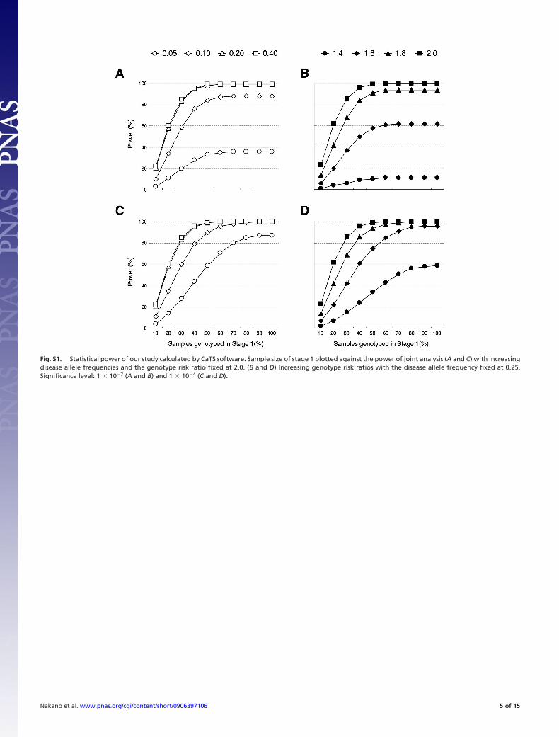
Fig. S1. Statistical power of our study calculated by CaTS software. Sample size of stage 1 plotted against the power of joint analysis (A and C) with increasingdisease allele frequencies and the genotype risk ratio fixed at 2.0. (B and D) Increasing genotype risk ratios with the disease allele frequency fixed at 0.25.Significance level: 1 � 10�7 (A and B) and 1 � 10�4 (C and D).

Nakano et al. www.pnas.org/cgi/content/short/0906397106 5 of 15

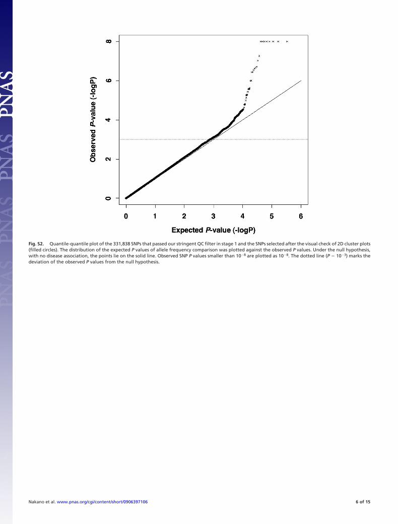
Fig. S2. Quantile-quantile plot of the 331,838 SNPs that passed our stringent QC filter in stage 1 and the SNPs selected after the visual check of 2D cluster plots(filled circles). The distribution of the expected P values of allele frequency comparison was plotted against the observed P values. Under the null hypothesis,with no disease association, the points lie on the solid line. Observed SNP P values smaller than 10�8 are plotted as 10�8. The dotted line (P � 10�3) marks thedeviation of the observed P values from the null hypothesis.

Nakano et al. www.pnas.org/cgi/content/short/0906397106 6 of 15

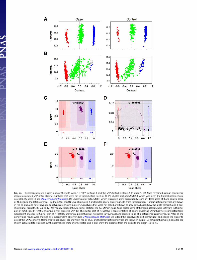
Fig. S3. Representative 2D cluster plots of the SNPs with P � 10�3 in stage 1 and the SNPs tested in stage 2. In stage 1, 255 SNPs remained as high-confidencedisease-associated SNPs after eliminating those that were not in tight clusters (see Fig. 1). (A) Cluster plot of rs7961953, which was given the highest possible totalacceptability score (4; see SI Materials and Methods). (B) Cluster plot of rs10764881, which was given a low acceptability score of 1 (case score of 0 and control scoreof 1). Because the total score was less than 2 for this SNP, we eliminated it and similar poorly clustering SNPs from consideration. Homozygotic genotypes are shownin red or blue, and heterozygotic genotypes are shown in green. Genotypes that were not called are shown as gray dots. X axes show the allele contrast, and Y axesshow signal strength. (C, D, E and F) We visually checked the 2D cluster plots for the 223 SNPs in stage 2 and edited some of them using BeadStudio software. (C) Clusterplot of rs7961953 (P � 0.05) showing a well-clustered SNP. (D) The cluster plot of rs1569868 is representative of poorly clustering SNPs that were eliminated fromsubsequent analysis. (E) Cluster plot of rs1819829 showing a point that was not called (arrowhead) and seemed to be of a heterozygous genotype. (F) After all thegenotyping results were checked by 3 independent observers (see SI Materials and Methods), we judged this genotype to be heterozygous and edited the cluster toaccept this SNP as shown. Homozygotic genotypes are shown in red or blue, and heterozygotic genotypes are shown in purple. Genotypes that were not called areshown as black dots. X axes show the normalized theta (Norm Theta), and Y axes show the distance from the point to the origin (Norm R).

Nakano et al. www.pnas.org/cgi/content/short/0906397106 7 of 15

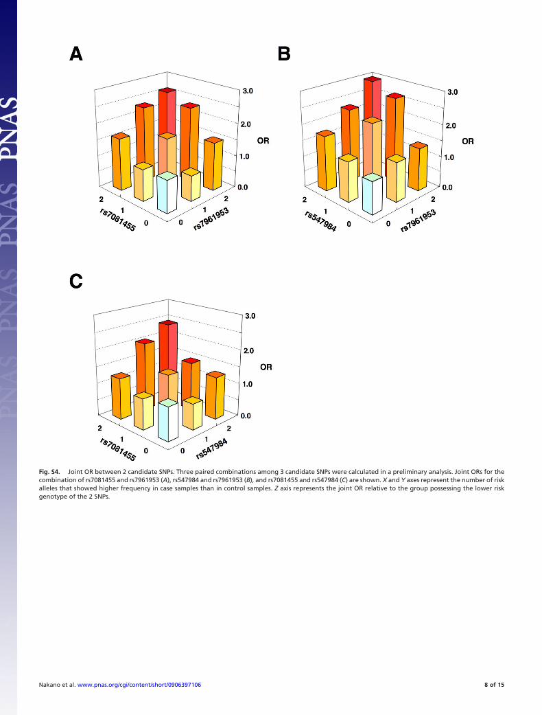
Fig. S4. Joint OR between 2 candidate SNPs. Three paired combinations among 3 candidate SNPs were calculated in a preliminary analysis. Joint ORs for thecombination of rs7081455 and rs7961953 (A), rs547984 and rs7961953 (B), and rs7081455 and rs547984 (C) are shown. X and Y axes represent the number of riskalleles that showed higher frequency in case samples than in control samples. Z axis represents the joint OR relative to the group possessing the lower riskgenotype of the 2 SNPs.

Nakano et al. www.pnas.org/cgi/content/short/0906397106 8 of 15

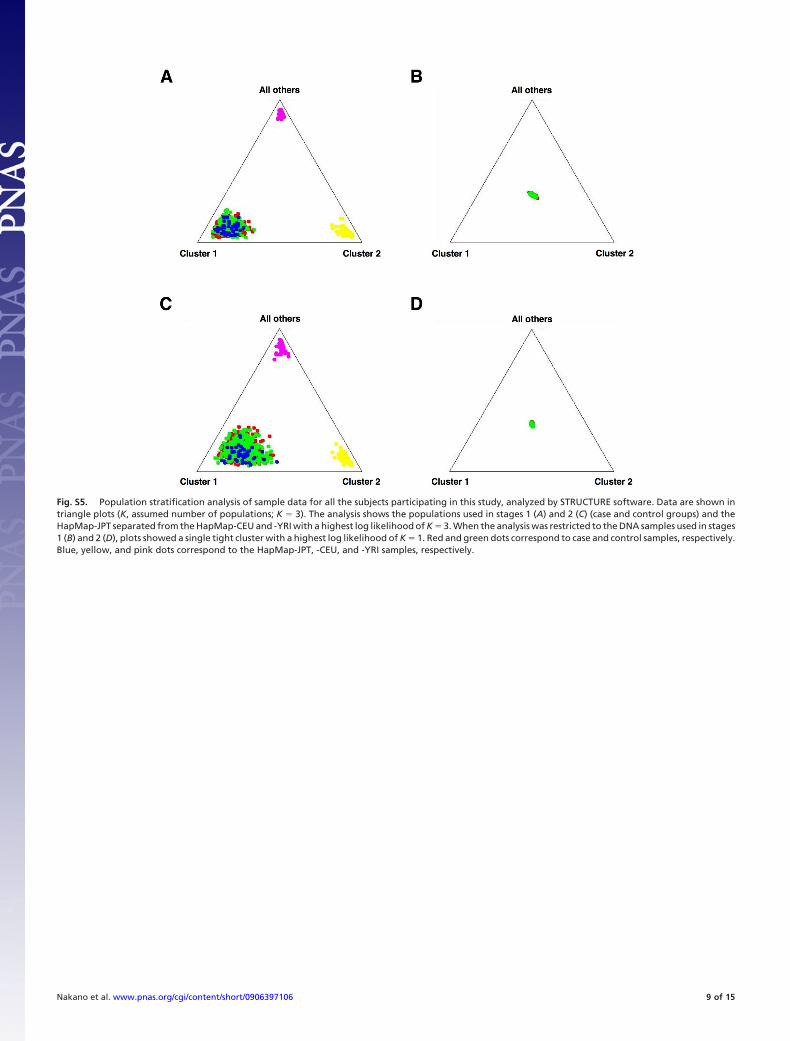
Fig. S5. Population stratification analysis of sample data for all the subjects participating in this study, analyzed by STRUCTURE software. Data are shown intriangle plots (K, assumed number of populations; K � 3). The analysis shows the populations used in stages 1 (A) and 2 (C) (case and control groups) and theHapMap-JPT separated from the HapMap-CEU and -YRI with a highest log likelihood of K � 3. When the analysis was restricted to the DNA samples used in stages1 (B) and 2 (D), plots showed a single tight cluster with a highest log likelihood of K � 1. Red and green dots correspond to case and control samples, respectively.Blue, yellow, and pink dots correspond to the HapMap-JPT, -CEU, and -YRI samples, respectively.

Nakano et al. www.pnas.org/cgi/content/short/0906397106 9 of 15

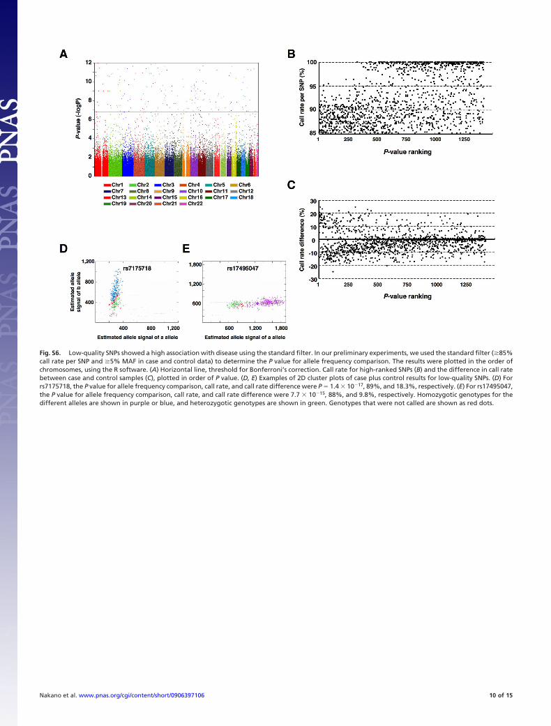
Fig. S6. Low-quality SNPs showed a high association with disease using the standard filter. In our preliminary experiments, we used the standard filter (�85%call rate per SNP and �5% MAF in case and control data) to determine the P value for allele frequency comparison. The results were plotted in the order ofchromosomes, using the R software. (A) Horizontal line, threshold for Bonferroni’s correction. Call rate for high-ranked SNPs (B) and the difference in call ratebetween case and control samples (C), plotted in order of P value. (D, E) Examples of 2D cluster plots of case plus control results for low-quality SNPs. (D) Forrs7175718, the P value for allele frequency comparison, call rate, and call rate difference were P � 1.4 � 10�17, 89%, and 18.3%, respectively. (E) For rs17495047,the P value for allele frequency comparison, call rate, and call rate difference were 7.7 � 10�15, 88%, and 9.8%, respectively. Homozygotic genotypes for thedifferent alleles are shown in purple or blue, and heterozygotic genotypes are shown in green. Genotypes that were not called are shown as red dots.

Nakano et al. www.pnas.org/cgi/content/short/0906397106 10 of 15

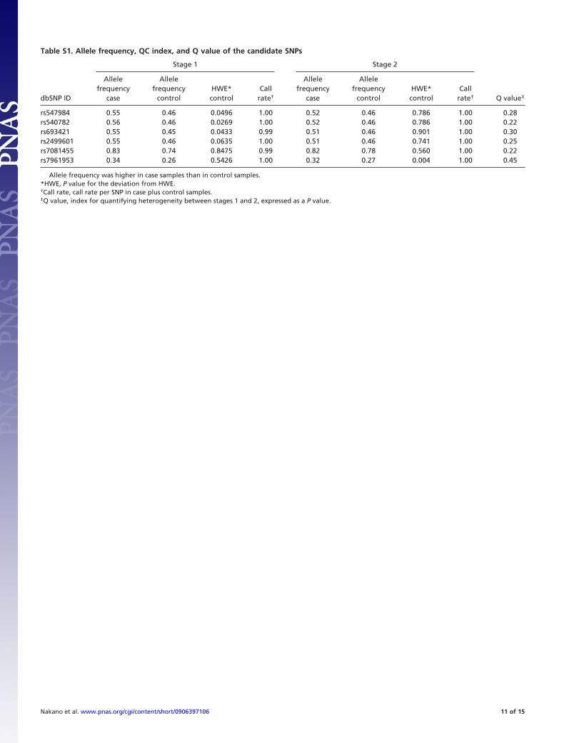
Table S1. Allele frequency, QC index, and Q value of the candidate SNPs

Stage 1 Stage 2

dbSNP ID

Allelefrequency

case

Allelefrequency

controlHWE*control

Callrate†

Allelefrequency

case

Allelefrequency

controlHWE*control

Callrate† Q value‡

rs547984 0.55 0.46 0.0496 1.00 0.52 0.46 0.786 1.00 0.28rs540782 0.56 0.46 0.0269 1.00 0.52 0.46 0.786 1.00 0.22rs693421 0.55 0.45 0.0433 0.99 0.51 0.46 0.901 1.00 0.30rs2499601 0.55 0.46 0.0635 1.00 0.51 0.46 0.741 1.00 0.25rs7081455 0.83 0.74 0.8475 0.99 0.82 0.78 0.560 1.00 0.22rs7961953 0.34 0.26 0.5426 1.00 0.32 0.27 0.004 1.00 0.45

Allele frequency was higher in case samples than in control samples.*HWE, P value for the deviation from HWE.†Call rate, call rate per SNP in case plus control samples.‡Q value, index for quantifying heterogeneity between stages 1 and 2, expressed as a P value.

Nakano et al. www.pnas.org/cgi/content/short/0906397106 11 of 15

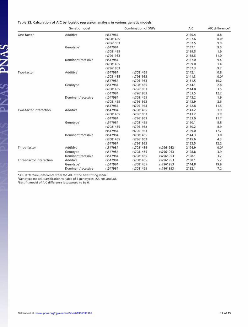
Table S2. Calculation of AIC by logistic regression analysis in various genetic models

Genetic model Combination of SNPs AIC AIC difference*

One-factor Additive rs547984 2166.4 8.8rs7081455 2157.6 0.0‡

rs7961953 2167.5 9.9Genotype† rs547984 2167.1 9.5

rs7081455 2159.5 1.9rs7961953 2168.6 11.0

Dominant/recessive rs547984 2167.0 9.4rs7081455 2159.0 1.4rs7961953 2167.3 9.7

Two-factor Additive rs547984 rs7081455 2142.1 0.8rs7081455 rs7961953 2141.3 0.0‡

rs547984 rs7961953 2151.5 10.2Genotype† rs547984 rs7081455 2144.1 2.8

rs7081455 rs7961953 2144.8 3.5rs547984 rs7961953 2153.5 12.2

Dominant/recessive rs547984 rs7081455 2143.2 1.9rs7081455 rs7961953 2143.9 2.6rs547984 rs7961953 2152.8 11.5

Two-factor interaction Additive rs547984 rs7081455 2143.2 1.9rs7081455 rs7961953 2143.2 1.9rs547984 rs7961953 2153.0 11.7

Genotype† rs547984 rs7081455 2150.1 8.8rs7081455 rs7961953 2150.2 8.9rs547984 rs7961953 2159.0 17.7

Dominant/recessive rs547984 rs7081455 2144.3 3.0rs7081455 rs7961953 2145.6 4.3rs547984 rs7961953 2153.5 12.2

Three-factor Additive rs547984 rs7081455 rs7961953 2124.9 0.0‡

Genotype† rs547984 rs7081455 rs7961953 2128.8 3.9Dominant/recessive rs547984 rs7081455 rs7961953 2128.1 3.2

Three-factor interaction Additive rs547984 rs7081455 rs7961953 2130.1 5.2Genotype† rs547984 rs7081455 rs7961953 2144.8 19.9Dominant/recessive rs547984 rs7081455 rs7961953 2132.1 7.2

*AIC difference, difference from the AIC of the best-fitting model.†Genotype model, classification variable of 3 genotypes: AA, AB, and BB.‡Best fit model of AIC difference is supposed to be 0.

Nakano et al. www.pnas.org/cgi/content/short/0906397106 12 of 15

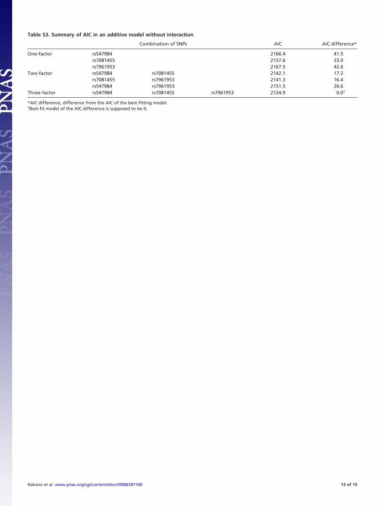
Table S3. Summary of AIC in an additive model without interaction

Combination of SNPs AIC AIC difference*

One-factor rs547984 2166.4 41.5rs7081455 2157.6 33.0rs7961953 2167.5 42.6

Two-factor rs547984 rs7081455 2142.1 17.2rs7081455 rs7961953 2141.3 16.4rs547984 rs7961953 2151.5 26.6

Three-factor rs547984 rs7081455 rs7961953 2124.9 0.0†

*AIC difference, difference from the AIC of the best-fitting model.†Best-fit model of the AIC difference is supposed to be 0.

Nakano et al. www.pnas.org/cgi/content/short/0906397106 13 of 15

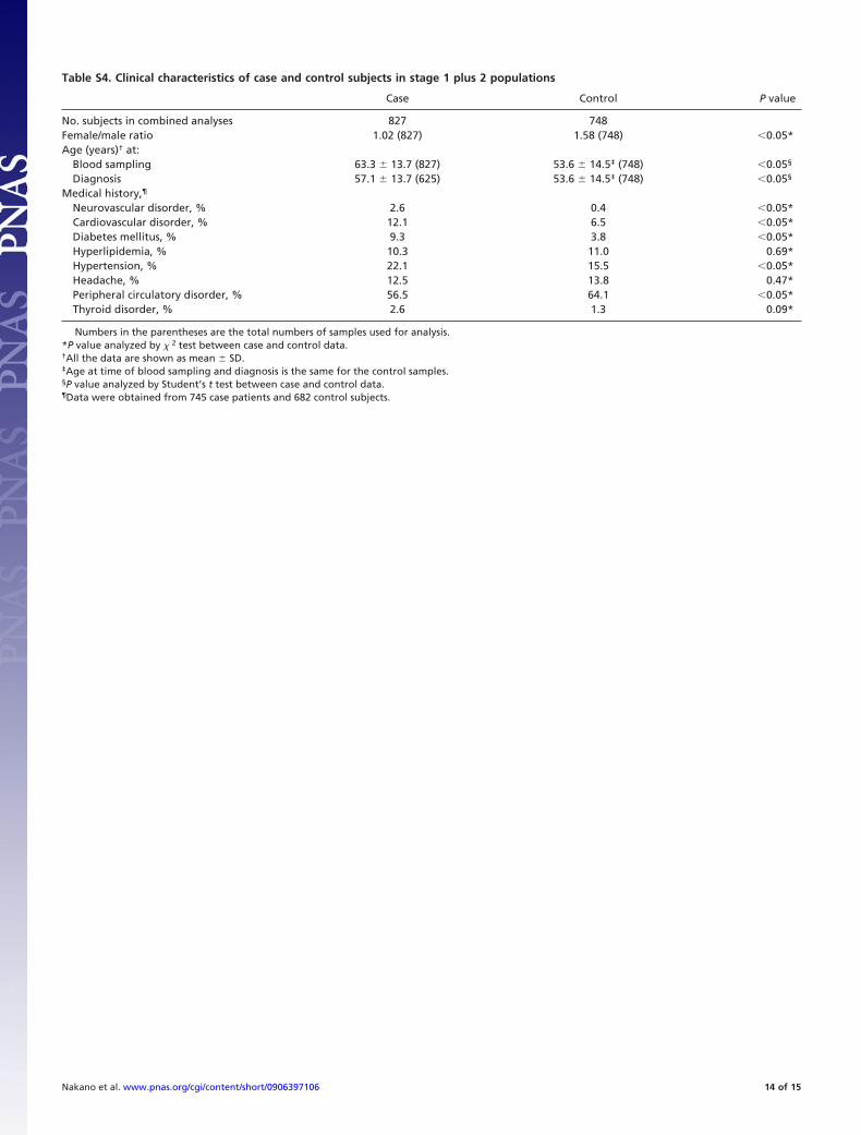
Table S4. Clinical characteristics of case and control subjects in stage 1 plus 2 populations

Case Control P value

No. subjects in combined analyses 827 748Female/male ratio 1.02 (827) 1.58 (748) �0.05*Age (years)† at:

Blood sampling 63.3 � 13.7 (827) 53.6 � 14.5‡ (748) �0.05§

Diagnosis 57.1 � 13.7 (625) 53.6 � 14.5‡ (748) �0.05§

Medical history,¶

Neurovascular disorder, % 2.6 0.4 �0.05*Cardiovascular disorder, % 12.1 6.5 �0.05*Diabetes mellitus, % 9.3 3.8 �0.05*Hyperlipidemia, % 10.3 11.0 0.69*Hypertension, % 22.1 15.5 �0.05*Headache, % 12.5 13.8 0.47*Peripheral circulatory disorder, % 56.5 64.1 �0.05*Thyroid disorder, % 2.6 1.3 0.09*

Numbers in the parentheses are the total numbers of samples used for analysis.*P value analyzed by � 2 test between case and control data.†All the data are shown as mean � SD.‡Age at time of blood sampling and diagnosis is the same for the control samples.§P value analyzed by Student’s t test between case and control data.¶Data were obtained from 745 case patients and 682 control subjects.

Nakano et al. www.pnas.org/cgi/content/short/0906397106 14 of 15

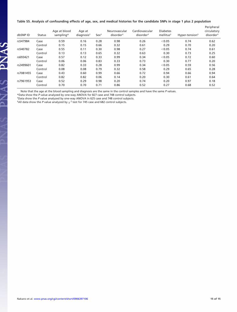
Table S5. Analysis of confounding effects of age, sex, and medical histories for the candidate SNPs in stage 1 plus 2 population

dbSNP ID StatusAge at blood

sampling*Age at

diagnosis† Sex‡

Neurovasculardisorder‡

Cardiovasculardisorder‡

Diabetesmellitus‡ Hyper-tension‡

Peripheralcirculatorydisorder‡

rs547984 Case 0.59 0.16 0.28 0.98 0.26 �0.05 0.74 0.62Control 0.15 0.15 0.66 0.32 0.61 0.29 0.70 0.20

rs540782 Case 0.55 0.11 0.30 0.98 0.27 �0.05 0.74 0.61Control 0.13 0.13 0.65 0.32 0.63 0.30 0.73 0.25

rs693421 Case 0.57 0.12 0.33 0.99 0.34 �0.05 0.72 0.60Control 0.06 0.06 0.83 0.33 0.73 0.30 0.77 0.20

rs2499601 Case 0.82 0.33 0.28 0.99 0.34 �0.05 0.59 0.56Control 0.08 0.08 0.79 0.32 0.58 0.29 0.65 0.28

rs7081455 Case 0.43 0.60 0.99 0.66 0.72 0.94 0.66 0.94Control 0.82 0.82 0.06 0.14 0.20 0.30 0.61 0.64

rs7961953 Case 0.52 0.29 0.98 0.20 0.74 0.20 0.97 0.18Control 0.70 0.70 0.71 0.86 0.52 0.27 0.68 0.52

Note that the age at the blood sampling and diagnosis are the same in the control samples and have the same P values.*Data show the P value analyzed by one-way ANOVA for 827 case and 748 control subjects.†Data show the P value analyzed by one-way ANOVA in 625 case and 748 control subjects.‡All data show the P value analyzed by � 2 test for 745 case and 682 control subjects.

Nakano et al. www.pnas.org/cgi/content/short/0906397106 15 of 15