supporting information supplementary results
TRANSCRIPT

Supporting Information
Supplementary results
This appendix was part of the submitted manuscript and has been peer reviewed. It is posted as supplied by the authors.
Appendix to: McBryde ES, Meehan MT, Caldwell JM, et al. Modelling direct and herd protection effects of vaccination against the SARS-CoV-2 Delta variant in Australia. Med J Aust 2021; doi: 10.5694/mja2.51263.

2
Modelling direct and herd protection effects of vaccination against
the SARS-CoV-2 Delta variant in Australia
1 Non-technical explanation of methods We build a 16 x 16 next generation matrix which provides the class-specific reproduction number for
each of 16 age classes {0-4, 5-9, 10-14,…,70-74, 75+}. For example, the value in row 0-4 column 0-4 is
the expected number of 0-4 year olds infected by a typical 0-4 year old case throughout their
infectious period.
To build this matrix, we start with the age-based contact matrix for Australia, published by Prem et
al. (2021) (1) which is also 16 x 16 and based on 5-year age groups, Figure 1, left panel. We modify
this by changing the risk of transmission per contact according to the age of the transmitter and the
age of the susceptible receiver of contacts (Davies et al. 2020, (2)). Each cell is then multiplied
through by the duration of infection and scaled to ensure that it calibrates to the effective
reproduction number under investigation, shown in Figure 1, right panel. It can be seen that the
highest transmitters are in the 15 to 50 year old groups.
Figure 1. Left panel provides the age specific contact matrix for Australia, based on data from Prem
et al. (2021). Right panel provides the next generation matrix further modified for infectiousness
susceptibility, duration of infection and scaling constant.
We then expand the matrix further to account for vaccinated and unvaccinated in each age group
(yielding a 32 x 32 element matrix) and apply the effects of vaccine on both susceptibility and
infectiousness to the next generation matrix.
From the next generation matrix, we can derive the effective reproduction number (as the dominant
eigenvalue) and the final size (total number of infections at the end of a completed epidemic) using
an adaptation of well-known final size methods, described in detail in section 2. This latter value is
age-specific and vaccine status-specific, allowing the following further estimates to be made: death
and hospitalisation rates modified by age and vaccination status, years of life lost, and relative
proportions of vaccinated and unvaccinated populations infected or dying.

3
2 Mathematical methods To model the transmission of SARS-CoV-2 we stratify the population into 16 5-year age bands 𝑎 ∈
{0 − 4, 5 − 9, 10 − 14, … , 70 − 74, 75+} and assume that individuals in age group 𝑎 possess a
relative susceptibility to infection 𝑢𝑎. Once infected, an age-dependent fraction 𝑦𝑎 go on to develop
symptomatic (i.e., clinical) disease whilst the remaining 1 − 𝑦𝑎 develop asymptomatic (i.e., sub-
clinical) disease. We assume that individuals in the sub-clinical class are less infectious than those in
the clinical class by a relative factor 𝑓 (baseline value 0.25 (2-7)) and that the total time spent
infectious for both classes is 𝜏 days.
Each day, each individual in age group 𝑎 makes 𝑐𝑎𝑎′ contacts with individuals in age group 𝑎′ leading
to the following expression for the (unscaled) next-generation matrix (NGM) (Diekmann et al. 2010
(8)):
�̅�𝑢𝑎𝑎′ =
𝑢𝑎𝑆𝑎𝑐𝑎𝑎′
𝑁𝑎′
[𝑦𝑎′ + (1 − 𝑦𝑎′)𝑓]𝜏
where 𝑆𝑎 is the number of susceptible individuals in age group 𝑎 and 𝑁𝑎′ is the total number of
individuals in age group 𝑎′. We allow that prior to vaccination an age-specific fraction 𝑝𝑎 of
individuals have immunity as a result of previous infection, such that 𝑆𝑎 = (1 − 𝑝𝑎)𝑁𝑎.
The (𝑎, 𝑎′)th entry of the 16 × 16 NGM �̅�𝑢 is proportional to the average number of new infections
in age group 𝑎 generated by an individual in age group 𝑎′ over their infectious lifetime. To calculate
the actual number of infections generated by each individual these entries must be scaled by the
(pseudo-)probability of transmission given contact, which we denote 𝜂. In particular, the effective
reproduction number in the absence of vaccination, 𝑅eff𝑣, which is proportional to the maximal
eigenvalue, or spectral radius of �̅�𝑢 (or 𝜌(𝐾𝑢)), can be expressed as
𝑅eff𝑣= 𝜂𝜌(�̅�𝑢) ⇒ 𝜂 =
𝑅eff𝑣
𝜌(�̅�𝑢)
Incorporating this definition of 𝜂 along with the possibility of pre-existing immunity 𝑝𝑎 the next-
generation matrix 𝐾𝑢 is given by
𝐾𝑢𝑎𝑎′ = 𝜂 ⋅
𝑢𝑎𝑆𝑎𝑐𝑎𝑎′
𝑁𝑎′
[𝑦𝑎′ + (1 − 𝑦𝑎′)𝑓]𝜏.
For a given 𝑅eff𝑣 we use the expression given above to calculate the scaling factor 𝜂 in terms of 𝑅eff𝑣
and 𝜌(�̅�𝑢). Daily, age-specific contact rates 𝑐𝑎𝑎′ are provided by the synthetic matrices presented in
(Prem et al. 2021).
2.1 Incorporating vaccination
In the presence of vaccination we further subdivide the population into those who are vaccinated
and those who are unvaccinated. Individuals who are vaccinated experience a reduced risk of
acquiring infection (by a factor 1 − 𝑉𝑎), a reduced risk of symptomatic disease (by a factor 1 − 𝑉𝑠),
a reduced risk of hospitalisation or death (by a factor 1 − 𝑉𝑚) and are potentially less infectious (by
a factor 1 − 𝑉𝑡). Each of these factors is dependent on the combination of SARS-CoV-2 strain and
vaccine. If a proportion 𝑣𝑎 of individuals in age group 𝑎 are vaccinated, then the modified 16 × 16
next-generation matrix in the presence of vaccination is given by

4
𝐾vac𝑎𝑎′ = 𝜂 ⋅
𝑢𝑎𝑆𝑎𝑐𝑎𝑎′
𝑁𝑎′
{[𝑦𝑎′ + (1 − 𝑦𝑎′)𝑓](1 − 𝑣𝑎′)
+ [(1 − 𝑉𝑠)𝑦𝑎′ + (1 − (1 − 𝑉𝑠)𝑦𝑎′)𝑓](1 − 𝑉𝑡)(1 − 𝑉𝑎)𝑣𝑎′}𝜏.
Note that this expression does not include the reduced risk of hospitalisation or death (1 − 𝑉𝑚) as
this is assumed to impact patient outcome only, and have no effect on transmission.
Further, this expression only stratifies the population according to age (i.e., the indices 𝑎, 𝑎′ only
index the 16 age groups introduced above). If we wish to additionally track the transmission rates
between individuals of different ages and different vaccination status, then we can use the
expanded (32 × 32) next-generation matrix �̃�, which can be expressed as the matrix product:
�̃� = [1 − 𝑣
(1 − 𝑉𝑎)𝑣] [𝐾𝑢 𝐾𝑣]
where the terms 1 − 𝑣 and (1 − 𝑉𝑎)𝑣 in the first factor are 16 × 16 diagonal matrices, the matrix
𝐾𝑢 is defined above and
𝐾𝑖𝑗𝑣 = 𝜂 ⋅
𝑢𝑖𝑆𝑖𝑐𝑖𝑗
𝑁𝑗[(1 − 𝑉𝑠 ⋅ 𝑣𝑗)𝑦𝑗 + (1 − (1 − 𝑉𝑠 ⋅ 𝑣𝑗)𝑦𝑗)𝑓](1 − 𝑉𝑡 ⋅ 𝑣𝑗)𝜏.
The indices 𝑖, 𝑗 in the expression above span the full set of 32 possible age-group x vaccination
categories.
2.2 Calculating the final size and disease-related mortality
To calculate the total number of infections and deaths throughout the course of an epidemic wave
we use the vectorised form of the final size equation given by (Andreasen 2011(9)):
1 − �̃�𝑖 = exp [−�̃�𝑖−1 ∑ �̃�𝑖𝑗�̃�𝑗�̃�𝑗
𝑗
]
where �̃�𝑖 is the fraction of individuals in group 𝑖 that become infected throughout the epidemic, �̃�𝑖 is
the population size of group 𝑖 and �̃�𝑖𝑗 is the extended next-generation matrix defined in the previous
section. Note that here we use the extended (32 × 32) next-generation matrix �̃�𝑖𝑗 that stratifies by
both age and vaccination status because the infection-fatality rate for vaccinated individuals is
reduced by a factor (1 − 𝑉𝑠) × (1 − 𝑉𝑚) relative to those that are unvaccinated. Moreover, the
population size �̃� = ((1 − 𝑣𝑎)𝑁𝑎 , 𝑣𝑎𝑁𝑎) is a combined vector of the number of vaccinated and
unvaccinated individuals in each age group.
Solving the final size equation numerically, we can determine the total number of deaths 𝐷 using the
following expression:
𝐷 = Unvaccinated deaths + Vaccinated deaths
= ∑ 𝑑𝑎𝑧𝑎𝑢(1 − 𝑣𝑎)(1 − 𝑝𝑎)𝑆𝑎
𝑎∈{0−4,…,75+}
+ ∑ 𝑑𝑎𝑧𝑎𝑣(1 − 𝑉𝑚)(1 − 𝑉𝑠)𝑣𝑎(1 − 𝑝𝑎)𝑆𝑎
𝑎∈{0−4,…,75+}
= ∑ 𝑑𝑎[𝑧𝑎𝑢(1 − 𝑣𝑎) + 𝑧𝑎
𝑣(1 − 𝑉𝑚)(1 − 𝑉𝑠)𝑣𝑎](1 − 𝑝𝑎)𝑆𝑎
𝑎∈{0−4,…,75+}
where 𝑑𝑎 is the age-specific infection-fatality rate (O’Driscoll et al. 2020(10), Fisman et al. 2021(11)),
and 𝑧𝑎𝑢 and 𝑧𝑎
𝑣 are the fractions of the unvaccinated and vaccinated populations in each age group

5
that become infected, respectively. The values 𝑑𝑎 are listed in Table 2. Using the total numbers of
deaths in each group and the life expectancy we also estimate the years of life lost (see Table 2).
Similarly, the total number of hospitalisation is calculated as
𝐻 = Unvaccinated hospitalisations + Vaccinated hospitalisations
= ∑ ℎ𝑎[𝑧𝑎𝑢(1 − 𝑣𝑎) + 𝑧𝑎
𝑣(1 − 𝑉𝑚)(1 − 𝑉𝑠)𝑣𝑎](1 − 𝑝𝑎)𝑆𝑎
𝑎∈{0−4,…,75+}
where ℎ𝑎 is the age-specific hospitalisation rate.
6
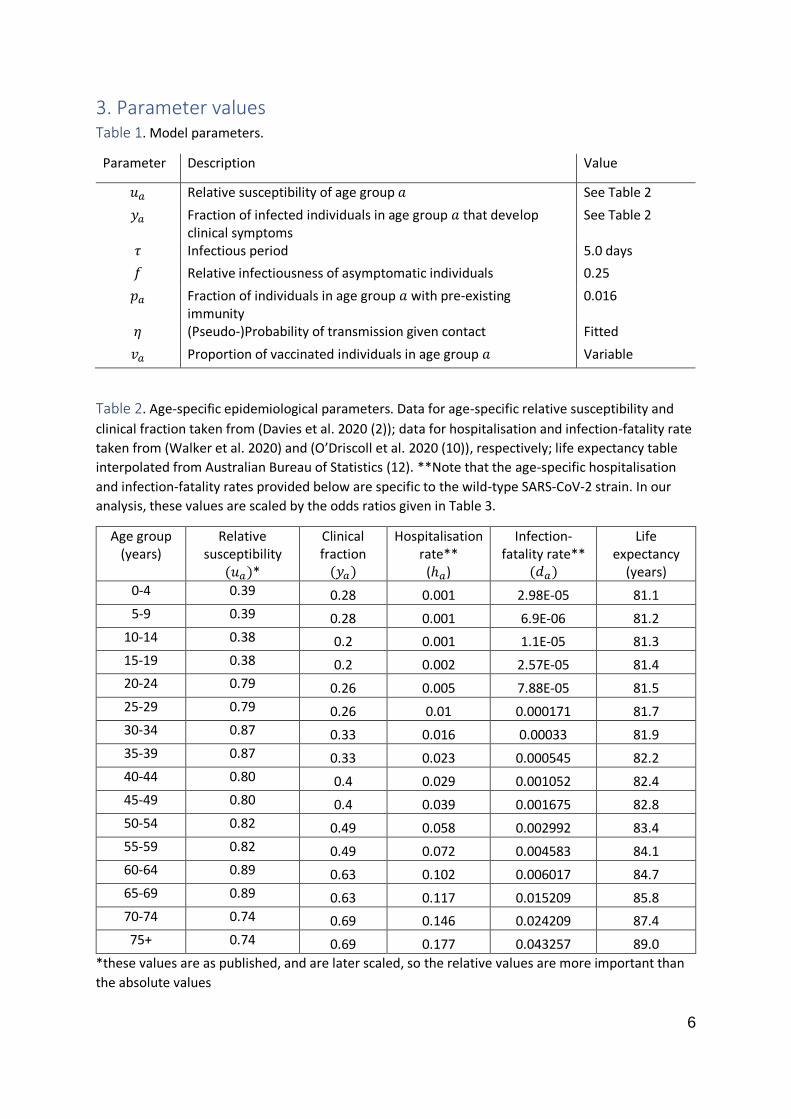
3. Parameter values Table 1. Model parameters.
Parameter Description Value
𝑢𝑎 Relative susceptibility of age group 𝑎 See Table 2
𝑦𝑎 Fraction of infected individuals in age group 𝑎 that develop clinical symptoms
See Table 2
𝜏 Infectious period 5.0 days
𝑓 Relative infectiousness of asymptomatic individuals 0.25
𝑝𝑎 Fraction of individuals in age group 𝑎 with pre-existing immunity
0.016
𝜂 (Pseudo-)Probability of transmission given contact Fitted
𝑣𝑎 Proportion of vaccinated individuals in age group 𝑎 Variable
Table 2. Age-specific epidemiological parameters. Data for age-specific relative susceptibility and
clinical fraction taken from (Davies et al. 2020 (2)); data for hospitalisation and infection-fatality rate
taken from (Walker et al. 2020) and (O’Driscoll et al. 2020 (10)), respectively; life expectancy table
interpolated from Australian Bureau of Statistics (12). **Note that the age-specific hospitalisation
and infection-fatality rates provided below are specific to the wild-type SARS-CoV-2 strain. In our
analysis, these values are scaled by the odds ratios given in Table 3.
Age group (years)
Relative susceptibility
(𝑢𝑎)*
Clinical fraction
(𝑦𝑎)
Hospitalisation rate**
(ℎ𝑎)
Infection-fatality rate**
(𝑑𝑎)
Life expectancy
(years)
0-4 0.39 0.28 0.001 2.98E-05 81.1
5-9 0.39 0.28 0.001 6.9E-06 81.2
10-14 0.38 0.2 0.001 1.1E-05 81.3
15-19 0.38 0.2 0.002 2.57E-05 81.4
20-24 0.79 0.26 0.005 7.88E-05 81.5
25-29 0.79 0.26 0.01 0.000171 81.7
30-34 0.87 0.33 0.016 0.00033 81.9
35-39 0.87 0.33 0.023 0.000545 82.2
40-44 0.80 0.4 0.029 0.001052 82.4
45-49 0.80 0.4 0.039 0.001675 82.8
50-54 0.82 0.49 0.058 0.002992 83.4
55-59 0.82 0.49 0.072 0.004583 84.1
60-64 0.89 0.63 0.102 0.006017 84.7
65-69 0.89 0.63 0.117 0.015209 85.8
70-74 0.74 0.69 0.146 0.024209 87.4
75+ 0.74 0.69 0.177 0.043257 89.0
*these values are as published, and are later scaled, so the relative values are more important than
the absolute values

7
Table 3. (Adjusted) Odds ratios for hospitalisation and infection for Delta variant relative to non-
VOC strains (Fisman et al. 2021 (11)).
Outcome Odds ratio (95% CI)
Hospitalisation 2.08 (1.80, 2.38)
Death 2.32 (1.47, 3.30)
Table 4. Vaccine efficacy.
Vaccine
Clinical trial efficacy
(𝑉𝑒) (95% CI)
Efficacy against
acquisition (𝑉𝑎)
Efficacy against symptomatic
disease (𝑉𝑠)
Efficacy against
transmission (𝑉𝑡)
Efficacy against severe disease
given symptomatic
disease (𝑉𝑚)
BNT162b2 (Pfizer)
0.880 (0.853, 0.901)
0.76 0.5 0.5 0.5
ChAdOx1 (AstraZeneca)
0.670 (0.613, 0.718)
0.48 0.37 0.5
0.8

8
4. Hospitalisation and deaths a. Coverage versus hospitalisations
b. Coverage versus deaths
Figure 2. Model predictions for the impact of different vaccine programs: Pfizer, AstraZeneca or
Mixed, indicated by column. Each is considered for values of 𝑅eff𝑣 of 3, 5 and 7, indicated by rows.
Vaccine uptake is fixed at 90%. For each subgraph there are three strategies (vulnerable,
transmitters and untargeted), indicated by colours, and two age of vaccine cut-offs (5 years and 15
years), indicated by line type. Panel a shows coverage versus hospitalisations and panel b shows
coverage versus deaths.

9
5. Sensitivity analysis Owing to the relatively recent emergence and dominance of the Delta variant of SARS-CoV-2, several
of the parameters used in our primary analysis remain considerably uncertain. Outcome sensitivity
to the most central of these, the effective reproduction number in the absence of vaccination (𝑅eff𝑣),
is explored in the main article; however, uncertainty in the remaining model parameters may still
have significant impacts on our results.
To encapsulate this uncertainty and explore their effect on each of our measured outcomes, we
conducted a Monte-Carlo-type sensitivity analysis where 1,000 parameter combinations were drawn
from the probability distributions described in Table 5 using Latin-Hypercube-Sampling. Given these
parameter combinations, we then forward-simulated our model (i.e., solved the generalised final
size equation) to calculate the cumulative number of infections, hospitalisations, deaths and years of
life lost. The results of this analysis are presented in Figure 3. Note, for clarity, we also reproduce the
first panel of Figure 3 (infections v. coverage) in Figure 4 using a discrete x-axis.
Table 5. Monte Carlo parameter distributions
Parameter Description Central estimate (95% CI) or (Range)
Monte Carlo distribution
𝑓 Relative infectiousness of asymptomatic individuals
0.25 (Range: 0.15, 1)
Triangular( Min = 0.15, Mode = 0.25, Max = 1 )
𝑉𝑒Pfizer Clinical efficacy of Pfizer at preventing symptomatic COVID-19
0.880 (95% CI: 0.853, 0.901)
Triangular( Min = 0.853, Mode = 0.880, Max = 0.901 )
𝑉𝑒AstraZeneca Clinical efficacy of AstraZeneca at preventing symptomatic COVID-19
0.670 (95% CI: 0.613, 0.718)
Triangular( Min = 0.613, Mode = 0.670, Max = 0.718 )
𝑂𝑅hospitalisation Odds ratio of hospitalisation for Delta variant (relative non-VOCs)
2.08 (95% CI: 1.80, 2.38)
Triangular( Min = 1.80, Mode = 2.08, Max = 2.38 )
𝑂𝑅death Odds ratio of death for Delta variant (relative non-VOCs)
2.32 (95% CI: 1.47, 3.30)
Triangular( Min = 1.47, Mode = 2.32, Max = 3.30 )
Note that overall vaccine efficacy 𝑉𝑒 is not a direct model input. Instead, we decompose this value
into a component responsible for conferring protection against acquisition of infection (𝑉𝑎), and the
remainder into conferring protection against developing symptomatic disease given infection (𝑉𝑠).

10
The decomposition is conducted randomly using a uniform distribution to first assign the value of 𝑉𝑎
(which ranges from 0.25 times the overall vaccine efficacy up to the overall vaccine efficacy):
𝑉𝑎 ∼ 𝑈(0.25 × 𝑉𝑒, 𝑉𝑒)
and then back-calculating 𝑉𝑠 to preserve the overall vaccine efficacy 𝑉𝑒:
𝑉𝑠 = 1 −1 − 𝑉𝑒
1 − 𝑉𝑎.
a. Coverage versus infections
b. Coverage versus hospitalisations

11
c. Coverage versus deaths
d. Coverage versus years of life lost
Figure 3. Sensitivity analysis for model predictions for the impact of different vaccine programs:
Pfizer, AstraZeneca or Mixed, indicated by column. Each is considered for values of 𝑅eff𝑣 of 3, 5 and
7, indicated by rows. Vaccine uptake is fixed at 90% and eligibility age at 15. For each subgraph there
are three strategies (vulnerable, transmitters and untargeted), indicated by colours. Panel a shows
coverage versus infections; panel b shows coverage versus hospitalisations; panel c shows coverage
versus deaths; and panel d shows coverage versus years of life lost. The central line in each subpanel
for each vaccination strategy gives the median outcome estimate across the range of sampled
parameters, whilst the upper and lower limits of each ribbon give the 95% central confidence
interval.

12
Figure 4. Reproduction of Figure 3, panel a using a discrete coverage lattice. Sensitivity analysis for
model predictions for the impact of different vaccine programs: Pfizer, AstraZeneca or Mixed,
indicated by column. Each is considered for values of 𝑅eff𝑣 of 3, 5 and 7, indicated by rows. Vaccine
uptake is fixed at 90% and eligibility age at 15. For each subgraph there are three strategies
(vulnerable, transmitters and untargeted), indicated by colours.
Incorporating uncertainty into the parameters described in Table 5, we find an apparent increase in
the overlap between the performance of each of the three vaccination strategies (untargeted,
vulnerable and transmitters) across the different outcomes; however, we emphasise that the ranking
described in the main article is largely preserved for fixed parameter values (e.g., equal vaccine
efficacy, relative infectiousness). Notably, the range of predicted values can vary considerably for
certain outcomes when parameter uncertainty is included; however, our conclusions regarding the
predicted capacity for vaccination to achieve herd immunity remain robust. That is, across the
parameter ranges considered, herd immunity remains unachievable for 𝑅eff𝑣≥ 5 whilst vaccine
eligibility is constrained to those over 15 years of age (which is the case for all panels in Figure 3.)

13
5.1 Contact matrix In a sensitivity analysis, we used an alternative approach to generate the age-specific contact rates 𝑐𝑖𝑗. These rates were obtained by extrapolating the contact rates estimated for the United Kingdom
(UK), where a contact survey was conducted in 2005-2006 (13). We used the R package socialmixr (v
0.1.8) to extract the UK age-specific contact rates (𝑐𝑖𝑗POLYMOD) emerging from the contact survey. We
then applied age-specific adjustments to account for age distribution differences between Australia and the UK, such that
𝑐𝑖𝑗 = 𝑐𝑖𝑗POLYMOD ×
𝜋𝑗AUS
𝜋𝑗UK
,
where 𝜋𝑗AUS and 𝜋𝑗
UK are the proportion of the population aged 𝑗 in Australia and the UK,
respectively. The results are shown in Figure 5.
a. Coverage versus infections
b. Coverage versus hospitalisations

14
c. Coverage versus deaths
d. Coverage versus years of life lost
Figure 5. Contact sensitivity analysis for model predictions for the impact of different vaccine
programs: Pfizer, AstraZeneca or Mixed, indicated by column. Each is considered for values of 𝑅eff𝑣
of 3, 5 and 7, indicated by rows. Vaccine uptake is fixed at 90% and eligibility age at 15. For each
subgraph there are three strategies (vulnerable, transmitters and untargeted), indicated by colours.
Panel a shows coverage versus infections; panel b shows coverage versus hospitalisations; panel c
shows coverage versus deaths; and panel d shows coverage versus years of life lost. The central line
in each subpanel for each vaccination strategy gives the median outcome estimate across the range
of sampled parameters, whilst the upper and lower limits of each ribbon give the 95% central
confidence interval.

15
References 1. Prem K, Zandvoort KV, Klepac P, et al; Centre for the Mathematical Modelling of Infectious
Diseases COVID-19 Working Group. Projecting contact matrices in 177 geographical regions: an
update and comparison with empirical data for the COVID-19 era. PLoS Comput Biol 2021; 17: e1009098.
2. Davies NG, Klepac P, Liu Y, et al. Age-dependent effects in the transmission and control of
COVID-19 epidemics. Nat Med 2020; 26: 1205-1211.
3. Buitrago-Garcia D, Egli-Gany D, Counotte MJ, et al. Occurrence and transmission potential of asymptomatic and presymptomatic SARS-CoV-2 infections: a living systematic review and meta-
analysis. PLoS Med 2020; 17: e1003346.
4. Nakajo K, Nishiura H. Transmissibility of asymptomatic COVID-19: data from Japanese clusters. Int J Infect Dis 2021; 105: 236-238.
5. Qiu X, Nergiz AI, Maraolo AE, et al. Defining the role of asymptomatic and pre-symptomatic
SARS-CoV-2 transmission: a living systematic review. Clin Microbiol Infect 2021; 27: 511-519.
6. Sayampanathan AA, Heng CS, Pin PH, et al. Infectivity of asymptomatic versus symptomatic COVID-19. Lancet 2021; 397: 93-94.
7. Yan D, Zhang X, Chen C, et al. Characteristics of viral shedding time in SARS-CoV-2
infections: a systematic review and meta-analysis. Front Public Health 2021; 9: 209.
8. Diekmann O, Heesterbeek JA, Roberts MG. The construction of next-generation matrices for
compartmental epidemic models. J R Soc Interface 2010; 7: 873-885.
9. Andreasen V. The final size of an epidemic and its relation to the basic reproduction number. Bull Math Biol 2011; 73: 2305-2321.
10. O’Driscoll M, Ribeiro Dos Santos G, Wang L, et al. Age-specific mortality and immunity
patterns of SARS-CoV-2. Nature 2021; 590: 140-145.
11. Fisman DN, Tuite AR. Progressive increase in virulence of novel SARS-CoV-2 variants in
Ontario, Canada [preprint], version 3. medRxiv 2021.07.05.21260050; 4 Aug 2021. doi:
https://doi.org/10.1101/2021.07.05.21260050 (viewed Aug 2021).
12. Australian Bureau of Statistics. Deaths in Australia. Updated 25 June 2021.
https://www.aihw.gov.au/reports/life-expectancy-death/deaths-in-australia/contents/life-expectancy
(viewed Aug 2021).
13. Mossong J, Hens N, Jit M, Beutels P, Auranen K, Mikolajczyk R, et al. Social contacts and
mixing patterns relevant to the spread of infectious diseases. PLoS Med 2008; 5: e74.