supporting information: in situ structure and dynamics...

Supporting Information: In situ structure anddynamics of DNA origami determined throughmolecular dynamics simulationsJejoong Yoo ∗ and Aleksei Aksimentiev ∗ †

∗Department of Physics and Center for the Physics of Living cells, University of Illinois at Urbana–Champaign, 1110 West Green Street, Urbana,Illinois 61801, and †Beckman Institute for Advanced Science and Technology

Submitted to Proceedings of the National Academy of Sciences of the United States of America

Design and simulation of the DNA origami structuresTo obtain fully atomistic models of DNA origami objects, we de-signed the target DNA origami structures using the caDNAno soft-ware, converted the caDNAno designs into all-atom representationsand refined the all-atom structures by performing MD simulations.

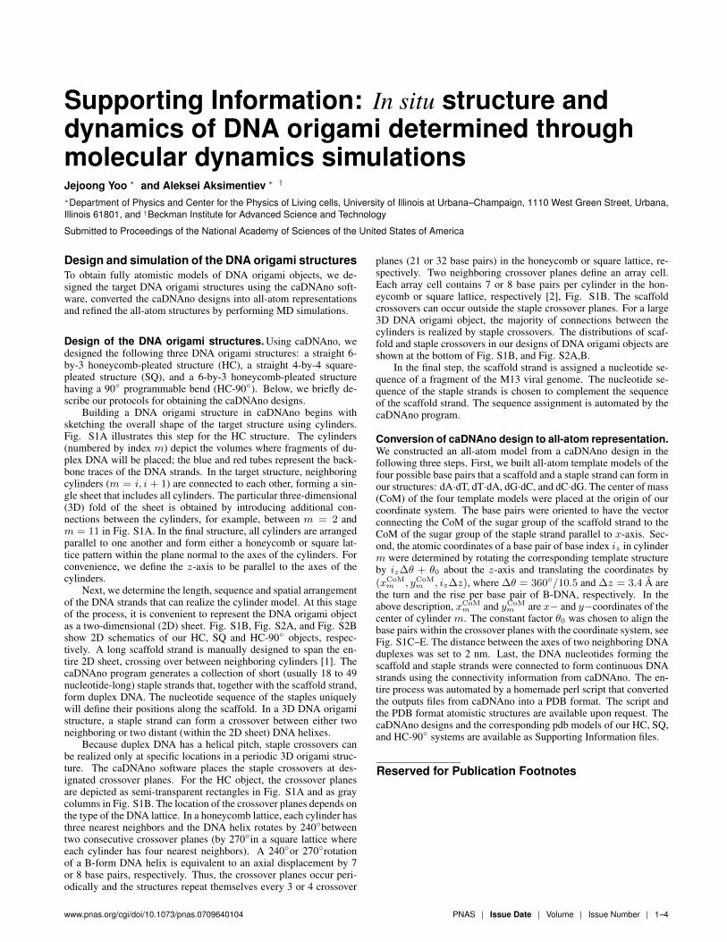
Design of the DNA origami structures. Using caDNAno, wedesigned the following three DNA origami structures: a straight 6-by-3 honeycomb-pleated structure (HC), a straight 4-by-4 square-pleated structure (SQ), and a 6-by-3 honeycomb-pleated structurehaving a 90◦ programmable bend (HC-90◦). Below, we briefly de-scribe our protocols for obtaining the caDNAno designs.

Building a DNA origami structure in caDNAno begins withsketching the overall shape of the target structure using cylinders.Fig. S1A illustrates this step for the HC structure. The cylinders(numbered by index m) depict the volumes where fragments of du-plex DNA will be placed; the blue and red tubes represent the back-bone traces of the DNA strands. In the target structure, neighboringcylinders (m = i, i + 1) are connected to each other, forming a sin-gle sheet that includes all cylinders. The particular three-dimensional(3D) fold of the sheet is obtained by introducing additional con-nections between the cylinders, for example, between m = 2 andm = 11 in Fig. S1A. In the final structure, all cylinders are arrangedparallel to one another and form either a honeycomb or square lat-tice pattern within the plane normal to the axes of the cylinders. Forconvenience, we define the z-axis to be parallel to the axes of thecylinders.

Next, we determine the length, sequence and spatial arrangementof the DNA strands that can realize the cylinder model. At this stageof the process, it is convenient to represent the DNA origami objectas a two-dimensional (2D) sheet. Fig. S1B, Fig. S2A, and Fig. S2Bshow 2D schematics of our HC, SQ and HC-90◦ objects, respec-tively. A long scaffold strand is manually designed to span the en-tire 2D sheet, crossing over between neighboring cylinders [1]. ThecaDNAno program generates a collection of short (usually 18 to 49nucleotide-long) staple strands that, together with the scaffold strand,form duplex DNA. The nucleotide sequence of the staples uniquelywill define their positions along the scaffold. In a 3D DNA origamistructure, a staple strand can form a crossover between either twoneighboring or two distant (within the 2D sheet) DNA helixes.

Because duplex DNA has a helical pitch, staple crossovers canbe realized only at specific locations in a periodic 3D origami struc-ture. The caDNAno software places the staple crossovers at des-ignated crossover planes. For the HC object, the crossover planesare depicted as semi-transparent rectangles in Fig. S1A and as graycolumns in Fig. S1B. The location of the crossover planes depends onthe type of the DNA lattice. In a honeycomb lattice, each cylinder hasthree nearest neighbors and the DNA helix rotates by 240◦betweentwo consecutive crossover planes (by 270◦in a square lattice whereeach cylinder has four nearest neighbors). A 240◦or 270◦rotationof a B-form DNA helix is equivalent to an axial displacement by 7or 8 base pairs, respectively. Thus, the crossover planes occur peri-odically and the structures repeat themselves every 3 or 4 crossover

planes (21 or 32 base pairs) in the honeycomb or square lattice, re-spectively. Two neighboring crossover planes define an array cell.Each array cell contains 7 or 8 base pairs per cylinder in the hon-eycomb or square lattice, respectively [2], Fig. S1B. The scaffoldcrossovers can occur outside the staple crossover planes. For a large3D DNA origami object, the majority of connections between thecylinders is realized by staple crossovers. The distributions of scaf-fold and staple crossovers in our designs of DNA origami objects areshown at the bottom of Fig. S1B, and Fig. S2A,B.

In the final step, the scaffold strand is assigned a nucleotide se-quence of a fragment of the M13 viral genome. The nucleotide se-quence of the staple strands is chosen to complement the sequenceof the scaffold strand. The sequence assignment is automated by thecaDNAno program.

Conversion of caDNAno design to all-atom representation.We constructed an all-atom model from a caDNAno design in thefollowing three steps. First, we built all-atom template models of thefour possible base pairs that a scaffold and a staple strand can form inour structures: dA·dT, dT·dA, dG·dC, and dC·dG. The center of mass(CoM) of the four template models were placed at the origin of ourcoordinate system. The base pairs were oriented to have the vectorconnecting the CoM of the sugar group of the scaffold strand to theCoM of the sugar group of the staple strand parallel to x-axis. Sec-ond, the atomic coordinates of a base pair of base index iz in cylinderm were determined by rotating the corresponding template structureby iz∆θ + θ0 about the z-axis and translating the coordinates by(xCoM

m , yCoMm , iz∆z), where ∆θ = 360◦/10.5 and ∆z = 3.4 Å are

the turn and the rise per base pair of B-DNA, respectively. In theabove description, xCoM

m and yCoMm are x− and y−coordinates of the

center of cylinder m. The constant factor θ0 was chosen to align thebase pairs within the crossover planes with the coordinate system, seeFig. S1C–E. The distance between the axes of two neighboring DNAduplexes was set to 2 nm. Last, the DNA nucleotides forming thescaffold and staple strands were connected to form continuous DNAstrands using the connectivity information from caDNAno. The en-tire process was automated by a homemade perl script that convertedthe outputs files from caDNAno into a PDB format. The script andthe PDB format atomistic structures are available upon request. ThecaDNAno designs and the corresponding pdb models of our HC, SQ,and HC-90◦ systems are available as Supporting Information files.

Reserved for Publication Footnotes

www.pnas.org/cgi/doi/10.1073/pnas.0709640104 PNAS Issue Date Volume Issue Number 1–4

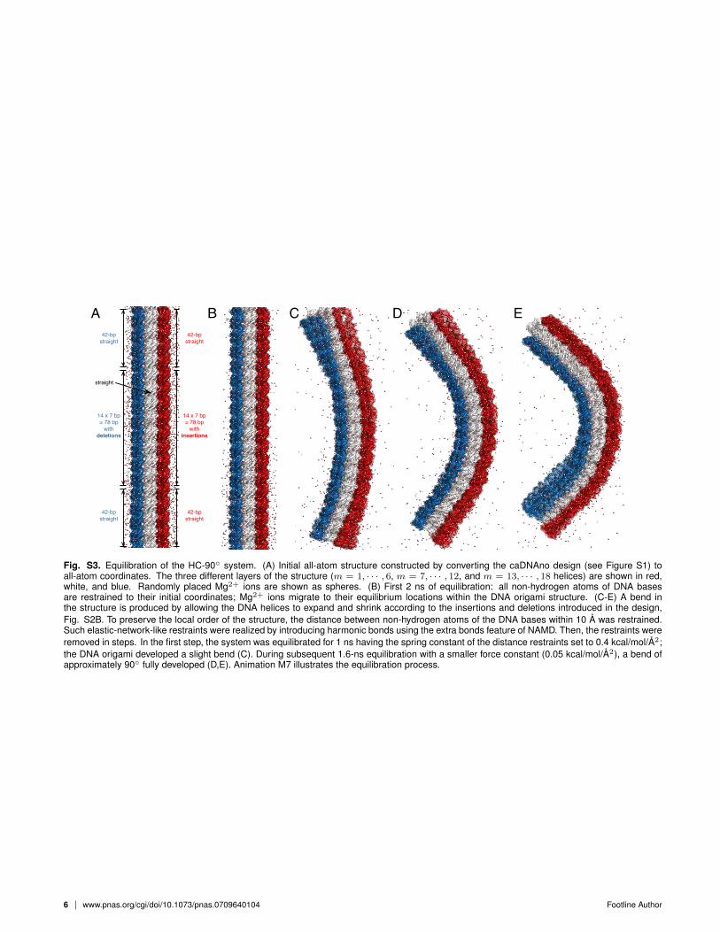
Multi-step equilibration of the HC-90◦structure.First, weequilibrated the HC-90◦system for 2 ns applying harmonic con-straints ( k = 1 kcal/mol/Å2) to all heavy atoms of DNA bases ina relatively small water box (∼ 14 × 15 × 60 nm3). During thisstep, Mg2+ ions redistributed within the origami, Fig. S3A,B. Fol-lowing that, the water box size was increased to∼ 26×18×60 nm3

by adding pre-equilibrated 10 mM solution of MgCl2, Fig. S3C. Toallow the helices carrying insertions or deletions to expand or shrink-ing while maintaining the local structural order, we used harmonicdistance restraints between all pairs of heavy atoms of DNA baseslocated within a 10 Å cutoff, Fig. S3 and Animation M7. Undersuch distance restraints, the system was equilibrated for 1 ns withthe spring constant of 0.4 kcal/mol/Å2, resulting in a slight bendingof the structure, Fig. S3C. The simulation was continued for 1.6 nswith k = 0.05 kcal/mol/Å2, which increased bending of the struc-ture Fig. S3D,E. At the end of the equilibration, HC-90◦ systemformed a bending angle of ∼90◦, Fig. S3E. The final conformationsof the equilibration simulations were used for production runs.

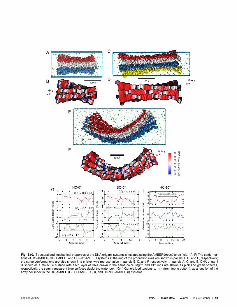
All-atom simulations using the AMBER99bsc0 force field.We also simulated our three DNA origami structures using the AM-BER99bsc0 DNA force field [3] in combination with the originalTIP3P water model [4] and ion parameters developed by Jeon etal. [5] and improved by Yoo et al. [6]. These simulations (sum-marized in Table S1) were performed using the Gromacs package [7].For our AMBER99bsc0 simulations, we used the same initial confor-mations, the same simulation parameters, and the same equilibrationprocedures as for our simulations that employed the CHARMM36force field. Specifically, the temperature was kept constant at 298 Kusing the Nosé-Hoover scheme [8, 9]. The pressure was kept constantat 1 bar using the Parrinello-Rahman scheme [10]. The grid size forthe Particle-Mesh Ewald summation was 1.2 Å [11].

The results of the AMBER99bsc0 simulations were consider-ably different from the results obtained using the CHARMM36force field. When simulated using the AMBER99bsc0 force field,the honeycomb-based structures developed significant twists (ω3 =2 − 4◦/cell) that were absent in our CHARMM36 simulations.Such twists are inconsistent with experimental measurements [1],Fig. S10G,I. Furthremore, the overall bending angle of the HC-90◦

structure converged to ∼120◦ in our AMBER99bsc0 simulations,which is also inconsistent with the experimentally determined angleof ∼90◦ [1], Fig. S10E,F. Thus, we found all-atom simulations ofDNA origami structures using the AMBER99bsc0 force field to ex-hibit considerable artifacts. Such artifacts were absent in analogoussimulations performed using CHARMM36.

Definition of triad vectorsFor our calculations of mechanical properties of monolith-like struc-tures, it was natural to define a contour, s = 0, . . . , L, parallel to the

central axis of each cylinder. Specifically, the contour was defined asa line that connects the CoMs of the neighboring array cells, Fig. 5A.For each array cell, we also defined a least-squares plane that mini-mizes the sum of distances to the CoMs of DNA in the same-indexcells. In Fig. 5A, the least-squares planes are shown in gray. Then,we defined a triad of unit vectors, {t̂i(s)|i = 1, 2, 3}, that werefixed in each array-cell plane (Fig. 4A inset). For the 6-by-3 hon-eycomb structure, t̂1 was parallel to the line connecting helix 7 and11, whereas t̂3 was normal to the plane and t̂2 = t̂3 × t̂1.

Animations of MD trajectoriesAnimation M1: HC-hbonds-layer1.mpg. This animation illus-trates the dynamics of base pairing at the single nucleotide level forthe first layer (m = 1 · · · 6) of the HC structure during the ∼130-nsproduction simulation. The backbone and bases of DNA are shownas tubes; each DNA strand has a unique color. Base pairs from thenon-peripheral region of the structure that remained broken for 10 nsor more are highlighted using the vdW (spheres) representations. Inframe zero, the circle indicates a base pair from array cell 6 thatbreaks and reforms during the simulation.

Animation M2: HC-hbonds-layer2.mpg.Same as AnimationM1 showing the second layer (m = 7 · · · 12) of the HC structure.

Animation M3: HC-hbonds-layer3.mpg.Same as AnimationM1 showing the third layer (m = 13 · · · 18) of the HC structure.

Animation M4: HC.mov. This animation illustrates the productionsimulation of the HC structure, covering∼130 ns. The DNA origamistructure is shown using a custom color-coded chicken wire represen-tation. The wire frame (black lines) connects the CoMs of the DNAbase pairs that form continuous double-stranded DNA cylinders ofthe original DNA origami designs. The lines between the CoMs ofthe same-index base pairs connect the wire frame. The length of thelines indicate the local inter-DNA distance, which is color-coded.

Animation M5: SQ.mov. This animation illustrates the productionsimulation of the SQ structure, covering∼120 ns. The DNA origamistructure is shown using a custom color-coded chicken wire repre-sentation as described for Animation 4.

Animation M6: HC90.mov. This animation illustrates the produc-tion simulation of the HC-90◦ structure, covering ∼30 ns. The DNAorigami structure is shown using a custom color-coded chicken wirerepresentation as described for Animation M4.

Animation M7: HC90-equil.mov. This animation illustrates theequilibration process that allows 90◦ bending of the HC-90◦ struc-ture.

1. Dietz H, Douglas SM, Shih WM (2009) Folding DNA into twisted and curvednanoscale shapes. Science 325(5941):725–30.

2. Douglas SM, et al. (2009) Rapid prototyping of 3D DNA-origami shapes with caD-NAno. Nucl Acids Res 37(15):5001–6.

3. Perez A, et al. (2007) Refinement of the AMBER force field for nucleic acids: Im-proving the description of α/γ conformers. Biophys J 92:3817–3829.

4. Jorgensen WL, Chandrasekhar J, Madura JD, Impey RW, Klein ML (1983) Com-parison of simple potential functions for simulating liquid water. J Chem Phys79(2):926–935.

5. Joung I, Cheatham T (2009) Molecular dynamics simulations of the dynamic andenergetic properties of alkali and halide ions using water-model-specific ion pa-rameters. J Phys Chem B 113(40):13279–90.

6. Yoo J, Aksimentiev A (2012) Improved parametrization of Li+, Na+, K+, and Mg2+

ions for all-atom molecular dynamics simulations of nucleic acid systems. J PhysChem Lett 3(1):45–50.

7. Hess B, Kutzner C, Van Der Spoel D, Lindahl E (2008) Gromacs 4: Algorithms forhighly efficient, load-balanced, and scalable molecular simulation. J Chem TheoryComput 4(3):435–447.

8. Nose S, Klein ML (1983) Constant pressure molecular dynamics for molecular sys-tems. Mol Phys 50:1055–76.

9. Hoover WG (1985) Canonical dynamics: Equilibrium phase-space distributions.Phys Rev A 31(3):1695–1697.

10. Parrinello M, Rahman A (1981) Polymorphic transitions in single crystals: A newmolecular dynamics method. J Appl Phys 52(12):7182–90.

11. Darden T, York D, Pedersen L (1993) Particle mesh ewald: An n log(n) method forewald sums in large systems. J Chem Phys 98(12):10089–92.

2 www.pnas.org/cgi/doi/10.1073/pnas.0709640104 Footline Author

Table S1. Production MD simulations of DNA origami objects.

System # Array cell # Cylinder # nucleotides # atoms # staplesSimulation Time (ns)

CHARMM AMBER

HC 11 6× 3 = 18 2,640 802,149 43 ∼140 ∼100

HC-90◦ 27 6× 3 = 18 6,420 2,799,156 87 ∼30 ∼30

SQ 16 4× 4 = 16 3,760 943,837 55 ∼120 ∼100

Footline Author PNAS Issue Date Volume Issue Number 3

C

D

D

A

crossover plane ii crossover plane iii

y

z

x

i ii iii i ii iii

1

23

45

6

13

1415

1617

18

1211

109

87

B

y

x

⊗

crossover plane i

18

17

16

15

14

13

12

11

10

9

8

7

6

5

4

3

2

1

E

i ii iii i ii iii i ii iii i

1 2 3 4 5 6 7 8 9 10 11array cell index

base index =

= 12

m =

m =

cross over plane =

y

z

x

F

= 5' end= 3' end

86420#

Cros

sove

r847770635649423528211470

Staples Scaffolds

Fig. S1. Construction of all-atom origami structure using the caDNAno design. (A) A 3D cartoon view of the 6-by-3 honeycomb-pleated origamidesign (HC). Cylinders (m = 1, · · · , 18) depict how DNA duplexes are organized into a 3D structure. For convenience, the DNA duplexes arealigned with the z-axis. Blue and red tubes illustrate the backbone traces of the cylinder-filling DNA strands. In this particular structure, sixconsecutive helices form one layer (m = 1, · · · , 6,m = 7, · · · , 12, and m = 13, · · · , 18); the three DNA layers fold into a multi-layer structure. Inour SQ structure (not shown), four helices form one layer and four layers form a 4-by-4 square-pleated structure. (B) Top. A 2D schematic viewof the paths the DNA strands form within the HC structure. The long blue path covering the entire space represents the scaffold DNA strand;all other short paths represent the staple strands [1]. In panel A, the scaffold and staple strands are represented by the blue and red tubes,respectively. The scaffold and staple paths cross over between cylinders at designated crossover planes. The crossover planes for staple strandsare depicted as semi-transparent gray planes and vertical gray lines in panels A and B, respectively. Bottom. The number of crossovers as afunction of base index for the HC system. (C–E) Atomistic representations of the HC structure at the three unique crossover planes for staplestrands. The nucleotides forming the scaffold and staple strands are shown in blue and red, respectively. (F) The final all-atom model of the HCsystem in an aqueous environment. The scaffold and staple strands are shown in blue and red molecular graphics representations, respectively.Mg2+ ions are shown as pink spheres; the water box is drawn as a semi-transparent blue surface.


86420#

Cros

sove

r

189168147126105846342210

Staples Scaffolds

6420#

Cros

sove

r

1281129680644832160

Staples Scaffolds

BProgrammed bending

E

Base index

A

Base index

Fig. S2. 2D caDNAno designs of the 4-by-4 square-pleated origami structure, SQ panel A, and of the 6-by-3 honeycomb-pleated origami havinga 90◦ bent, HC-90◦ panel B. The long blue paths represent the scaffold DNA strands whereas the short paths of other colors represent the staplestrands. The loops and crosses in panel B indicate insertions and deletions, respectively. At the bottom of each panel, the number of scaffold(blue bars) and staple (red bars) crossovers is shown as a function of base index.


42-bpstraight

14 x 7 bp= 78 bp

with deletions

14 x 7 bp= 78 bp

with insertions

42-bpstraight

42-bpstraight

42-bpstraight

straight

A B C D E

Fig. S3. Equilibration of the HC-90◦ system. (A) Initial all-atom structure constructed by converting the caDNAno design (see Figure S1) toall-atom coordinates. The three different layers of the structure (m = 1, · · · , 6, m = 7, · · · , 12, and m = 13, · · · , 18 helices) are shown in red,white, and blue. Randomly placed Mg2+ ions are shown as spheres. (B) First 2 ns of equilibration: all non-hydrogen atoms of DNA basesare restrained to their initial coordinates; Mg2+ ions migrate to their equilibrium locations within the DNA origami structure. (C-E) A bend inthe structure is produced by allowing the DNA helices to expand and shrink according to the insertions and deletions introduced in the design,Fig. S2B. To preserve the local order of the structure, the distance between non-hydrogen atoms of the DNA bases within 10 Å was restrained.Such elastic-network-like restraints were realized by introducing harmonic bonds using the extra bonds feature of NAMD. Then, the restraints wereremoved in steps. In the first step, the system was equilibrated for 1 ns having the spring constant of the distance restraints set to 0.4 kcal/mol/Å2;the DNA origami developed a slight bend (C). During subsequent 1.6-ns equilibration with a smaller force constant (0.05 kcal/mol/Å2), a bend ofapproximately 90◦ fully developed (D,E). Animation M7 illustrates the equilibration process.


100

95

90

85

80

End-

end

angl

e (°)

302520151050Time (ns)

180

178

176

174

172

170

End-

end

angl

e (°)

100806040200Time (ns)

A B

6420

1412108642

50

141312111098765432

C

141312111098765432

y (n

m)

1412108642x (nm)

2520151050

86420

12108642

840

12

11

10

9

8

7

6

5

4

3

2

1

D23 – 24 Å

12

11

10

9

8

7

6

5

4

3

2

1

y (n

m)

12108642x (nm)

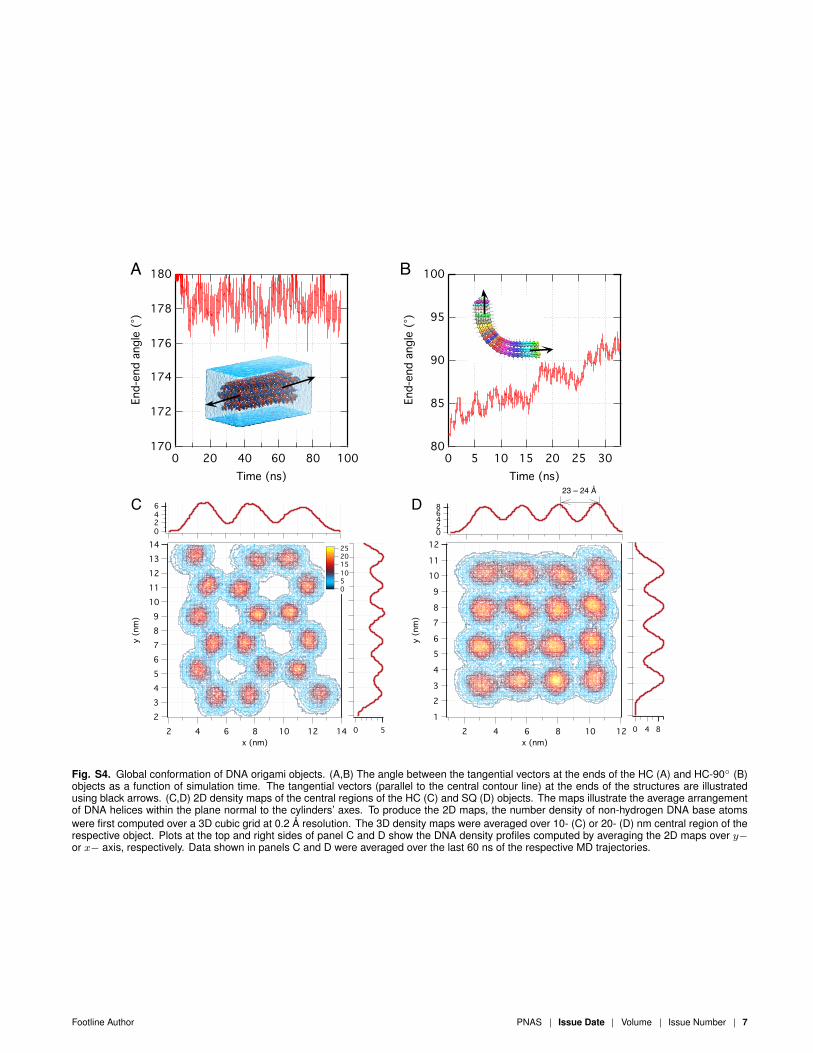
Fig. S4. Global conformation of DNA origami objects. (A,B) The angle between the tangential vectors at the ends of the HC (A) and HC-90◦ (B)objects as a function of simulation time. The tangential vectors (parallel to the central contour line) at the ends of the structures are illustratedusing black arrows. (C,D) 2D density maps of the central regions of the HC (C) and SQ (D) objects. The maps illustrate the average arrangementof DNA helices within the plane normal to the cylinders’ axes. To produce the 2D maps, the number density of non-hydrogen DNA base atomswere first computed over a 3D cubic grid at 0.2 Å resolution. The 3D density maps were averaged over 10- (C) or 20- (D) nm central region of therespective object. Plots at the top and right sides of panel C and D show the DNA density profiles computed by averaging the 2D maps over y−or x− axis, respectively. Data shown in panels C and D were averaged over the last 60 ns of the respective MD trajectories.


1.0

0.8

0.6

0.4

0.2

0.0

Conc

entr

atio

n (M

)

121086420

Distance from center (nm)

2[Mg] [P]

0.02

0.01

0.0011109876

[Mg] [P]

A B 7

6

5

4

3

2

1

0

Radi

al d

istrib

utio

n fu

nctio

n

1.00.90.80.70.60.50.4

P-Mg distance (nm)

P-Mg

[PO4]

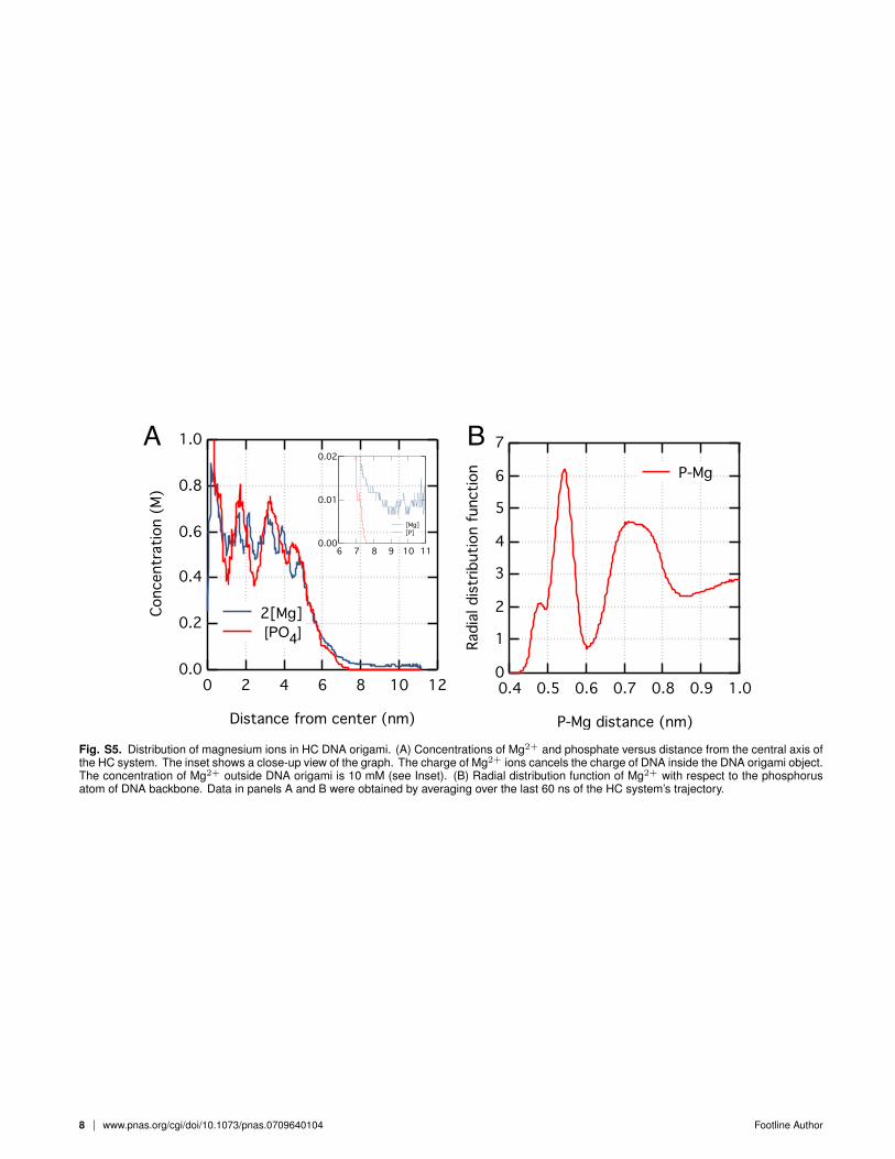
Fig. S5. Distribution of magnesium ions in HC DNA origami. (A) Concentrations of Mg2+ and phosphate versus distance from the central axis ofthe HC system. The inset shows a close-up view of the graph. The charge of Mg2+ ions cancels the charge of DNA inside the DNA origami object.The concentration of Mg2+ outside DNA origami is 10 mM (see Inset). (B) Radial distribution function of Mg2+ with respect to the phosphorusatom of DNA backbone. Data in panels A and B were obtained by averaging over the last 60 ns of the HC system’s trajectory.


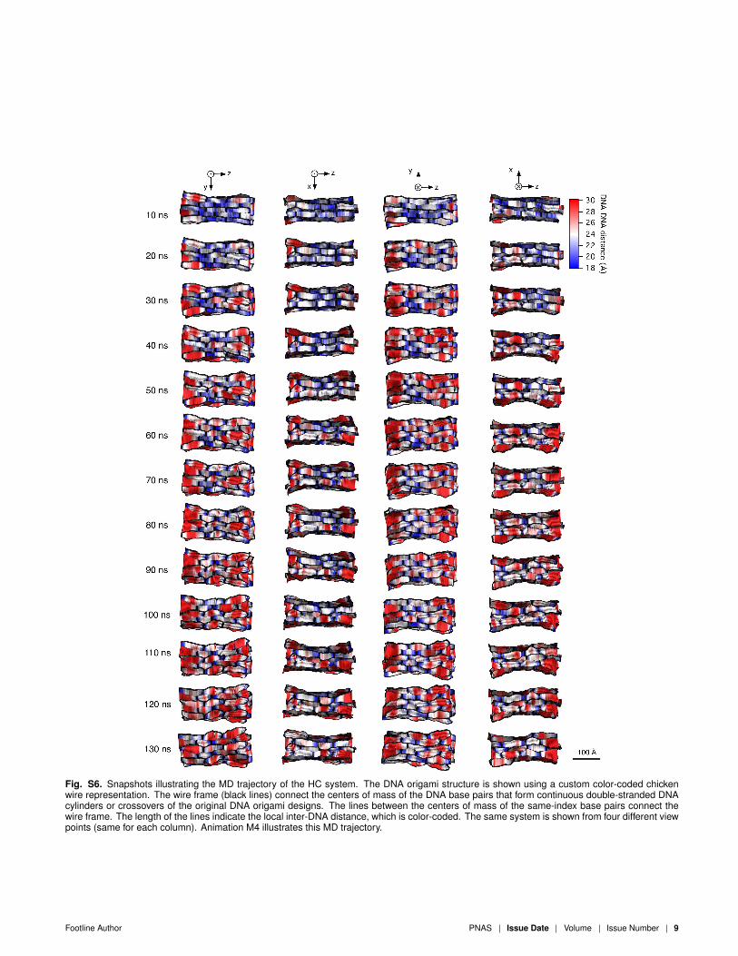
Fig. S6. Snapshots illustrating the MD trajectory of the HC system. The DNA origami structure is shown using a custom color-coded chickenwire representation. The wire frame (black lines) connect the centers of mass of the DNA base pairs that form continuous double-stranded DNAcylinders or crossovers of the original DNA origami designs. The lines between the centers of mass of the same-index base pairs connect thewire frame. The length of the lines indicate the local inter-DNA distance, which is color-coded. The same system is shown from four different viewpoints (same for each column). Animation M4 illustrates this MD trajectory.


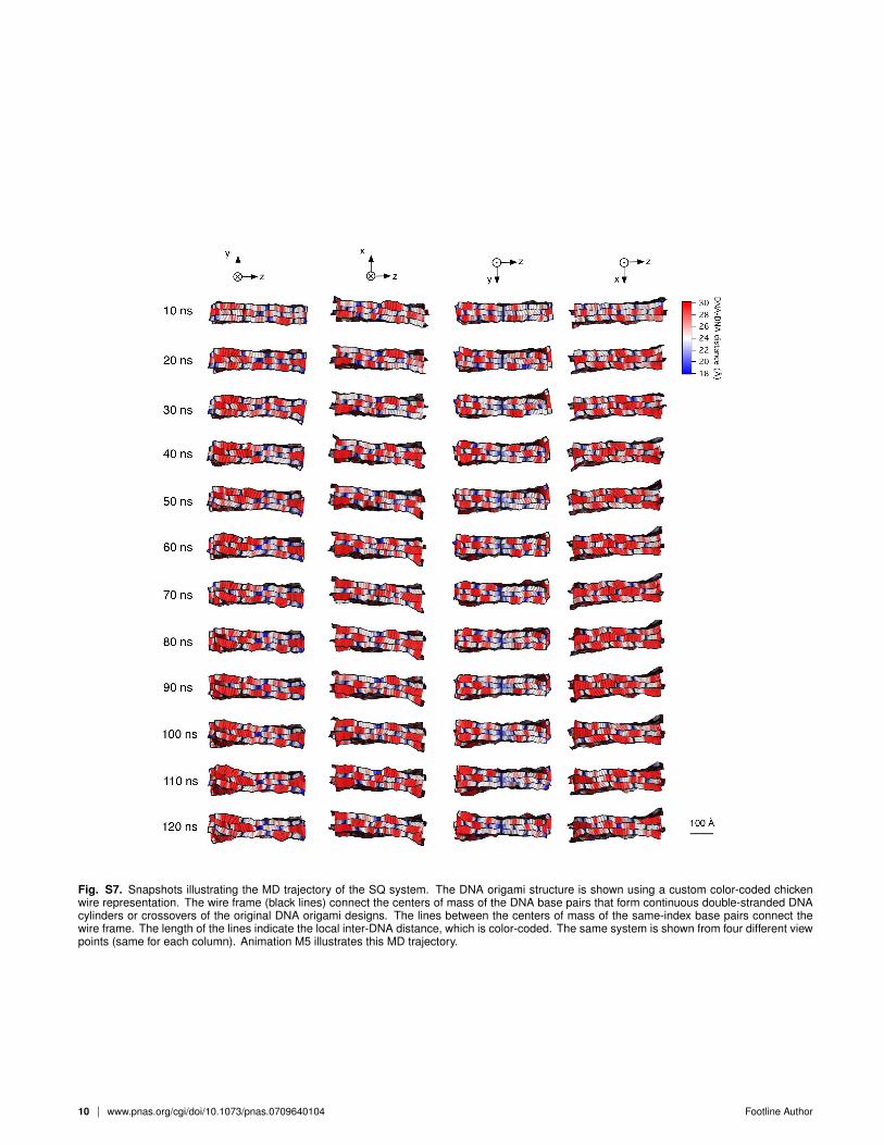
Fig. S7. Snapshots illustrating the MD trajectory of the SQ system. The DNA origami structure is shown using a custom color-coded chickenwire representation. The wire frame (black lines) connect the centers of mass of the DNA base pairs that form continuous double-stranded DNAcylinders or crossovers of the original DNA origami designs. The lines between the centers of mass of the same-index base pairs connect thewire frame. The length of the lines indicate the local inter-DNA distance, which is color-coded. The same system is shown from four different viewpoints (same for each column). Animation M5 illustrates this MD trajectory.


0.03

0.02

0.01

0.00

Prob

abilit

y De

ns. F

unc.

-60 -30 0 30 60Dihedral Angle (º)

Mean = -8.2° (± 15.6)

0.04

0.03

0.02

0.01

0.00

Prob

abilit

y De

ns. F

unc.

1801501209060300Angle (º)

24.4° (±11.4)143.5° (±12.7)

1.0

0.8

0.6

0.4

0.2

0.0

Prob

abilit

y De

ns. F

unc.

20161284Distance (Å)

4.5 Å (±0.7) 18.8 Å (±0.7)

jk'

l'i

j'k

li'

Distance (Å)

Angle (degree) Dihedral angle(degree)

A B

C D

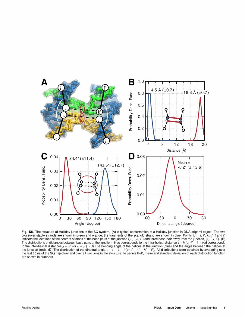
Fig. S8. The structure of Holliday junctions in the SQ system. (A) A typical conformation of a Holliday junction in DNA origami object. The twocrossover staple strands are shown in green and orange; the fragments of the scaffold strand are shown in blue. Points i, i′, j, j′, k, k′, l and l′indicate the locations of the centers of mass of the base pairs at the junction (j, j′, k, k′) and three base-pair away from the junction, (i, i′, l, l′). (B)The distributions of distances between base pairs at the junction. Blue corresponds to the intra-helical distance j− k (or j′− k′); red correspondsto the inter-helical distances j − k′ (or k − j′). (C) The bending angle of the helices at the junction (blue) and the angle between the helices atthe junction (red). (D) The distribution of the dihedral angle i − j − k − l (or i′ − j′ − k′ − l′). All distributions were obtained by averaging overthe last 60 ns of the SQ trajectory and over all junctions in the structure. In panels B–D, mean and standard deviation of each distribution functionare shown in numbers.


10080604020

0

µm

1086420

Array cell index

Mean = 47.7 ± 20.3

10080604020

0

µm

1086420

Array cell index

Mean = 59.0 ± 30.6

1086420

µm

1086420

Array cell index

Mean = 3.3 ± 1.7

↵1 (µm)

↵2 (µm)

↵3 (µm)

10080604020

0

µm

1612840

Array cell index

Mean = 34.6 ± 14.7

10080604020

0

µm

1612840

Array cell index

Mean = 25.5 ± 12.4

1086420

µm

1612840

Array cell index

Mean = 2.8 ± 1.1

↵1 (µm)

↵2 (µm)

↵3 (µm)

D E F

2500

2000

1500

1000

500

0

Coun

ts

-2 -1 0 1 2

Torsion (º/cell)

w1

2500

2000

1500

1000

500

0

Coun

ts

-2 -1 0 1 2

Torsion (º/cell)

w21000

800

600

400

200

0

Coun

ts

-10 -5 0 5 10

Torsion (º/cell)

w3

A B C!1 (�/cell) !2 (�/cell) !3 (�/cell)

Torsion (degree/cell) Torsion (degree/cell) Torsion (degree/cell)

Fig. S9. (A–C) Representative distributions of generalized torsions, ω1, ω2, and ω3. Histograms of torsions ω1 (A), ω2 (B), and ω3 (C) betweenarray cells 4 and 5 of the HC system (symbols). Gaussian fits to the histograms are shown as solid lines. (D–F) Bending (α1,2) and twist (α3)moduli in the HC (D), SQ (E), and HC-90◦ (F) structures as a function of the array cell index.


A

B

C

D

E

-8-404

° / c

ell

24201612840Array cell index

H

F

!1 (�/cell)

!2 (�/cell)

!3 (�/cell)

I!1 (�/cell)

!2 (�/cell)

!3 (�/cell)

HC-0° HC-90°SQ-0°

-2-1012

° / c

ell


-10-505

10

° / c

ell


Programmed bending

Gen

eral

ized

tors

ion

(°/c

ell)

G

Gen

eral

ized

tors

ion

(°/c

ell)

Gen

eral

ized

tors

ion

(°/c

ell)

zx⊗

zx⊗

zx⊗F

100

80

60

40

20

0100806040200

30282624222018

DNA-DNA distance (Å)

100 Å 100 Å

100 Å

Fig. S10. Structural and mechanical properties of the DNA origami systems simulated using the AMBER99bsc0 force field. (A–F) The conforma-tions of HC-AMBER, SQ-AMBER, and HC-90◦-AMBER systems at the end of the production runs are shown in panels A, C, and E, respectively;the same conformations are also shown in a chickenwire represenation in panels B, D, and F, respectively. In panels A, C, and E, DNA origamiis shown as a molecule surface with each layer of DNA drawn in the same color; Mg2+ and Cl− ions are shown as pink and green spheres,respectively; the semi-transparent blue surfaces depict the water box. (G–I) Generalized torsions, ω1,2,3 (from top to bottom), as a function of thearray cell index in the HC-AMBER (G), SQ-AMBER (H), and HC-90◦-AMBER (I) systems.


supporting information: in situ structure and dynamics...

Documents