supply chain network design under profit maximization and
TRANSCRIPT

Supply Chain Network Design
Under
Profit Maximization and Oligopolistic Competition
Anna Nagurney
Department of Finance and Operations Management
Isenberg School of Management
University of Massachusetts
Amherst, Massachusetts 01003
e-mail: [email protected]
phone: 413-545-5635
fax: 413-545-3858
July 2009; revised October 2009
Transportation Research E (2010) 46, 281-294.
Abstract: In this paper, we model the supply chain network design problem with oligopolis-
tic firms who are involved in the competitive production, storage, and distribution of a homo-
geneous product to multiple demand markets. The profit-maximizing firms select both the
capacities associated with the various supply chain network activities as well as the product
quantities. We formulate the governing Nash-Cournot equilibrium conditions as a variational
inequality problem and identify several special cases of the model, notably, a generalization
of a spatial oligopoly and a classical oligopoly problem to include design capacity variables.
The proposed computational approach, which is based on projected dynamical systems, fully
exploits the network structure of the problems and yields closed form solutions at each it-
eration. In order to illustrate the modeling framework and the algorithm, we also provide
solutions to a spectrum of numerical supply chain network oligopoly design examples.
This paper makes a contribution to game theoretic modeling of competitive supply chain
network design problems in an oligopolistic setting.
Keywords: profit-maximizing supply chains, supply chain design, network oligopolies, game
theory, Nash equilibria, variational inequalities, projected dynamical systems
1

1. Introduction
Oligopolies are a fundamental economic organizational structure and capture numerous
industries and their associated products and services ranging from airlines to particular re-
tailers as well as high technology manufacturers, telecommunication companies, and specific
energy providers. Hence, the formulation, analysis, and solution of oligopoly problems are all
of wide theoretical and application-based interest in both economics and operations research
(cf. Gabay and Moulin (1980), Murphy, Sherali, and Soyster (1982), Dafermos and Nagur-
ney (1987), Tirole (1988), Flam and Ben-Israel (1990), Okuguchi and Szidarovsky (1990),
Nagurney (1993, 2006a), Nagurney, Dupuis, and Zhang (1994), and the references therein).
In addition, there has been growing interest in the modeling of oligopolies in a supply chain
network context, derived, in part, from the recent, notable mergers and acquisitions of firms
in such industries as: beverage, airline, financial services, and oil (cf. Nagurney (2009a),
Nagurney and Qiang (2009), and the references therein), and the associated need to be able
to identify and quantify potential synergies.
In particular, in this paper, we consider the modeling of the explicit supply chain net-
work design problem in the context of oligopolies consisting of firms who compete in a Nash
(1950, 1951)-Cournot (1838) framework. As noted in Brown et al. (2001), more firms now
understand the potential benefits of controlling the supply chain as a whole. In this paper,
we assume that the firms produce a homogeneous good and compete in a noncooperative
manner. As in Nagurney (2009a,b), we depict each firm as a network of its economic activ-
ities of production, storage, and distribution to demand markets. Of course, the modeling
of mergers and acquisitions in a supply chain network context (cf. Nagurney (2009a,b),
Nagurney, Woolley, and Qiang (2009), and Nagurney and Woolley (2009)) may be viewed
as a supply chain network design problem, broadly classified. However, in this paper, we
make explicit the design variables associated with profit-maximizing, competing firms and
their supply chains.
The supply chain network design model developed in this paper extends the aforemen-
tioned supply chain network models in several significant ways. First, here we explicitly
consider oligopolistic behavior and associate demand market price functions with the de-
mand markets, whereas Nagurney (2009b) assumed known demands and assumed that the
2
link capacities were fixed and assigned a priori. In addition, we extend the (pre-merger)
oligopolistic supply chain network model of Nagurney (2009a), substantively, by allowing
for competition on the production side, in distribution and storage, and, finally, across the
demand markets. Moreover, the capacities are now strategic decision variables. Finally, we
also extend the original supply chain network design model of Nagurney (2009c), in which
there is a single, cost-minimizing firm faced with known demands at the markets for its prod-
uct and, hence, there is no competition. For flexibility, clarity, and continuity, the multifirm,
multimarket, supply chain network design model developed in this paper is formulated as
a variational inequality problem (cf. the book by Nagurney (1993), which also contains
some of the history of the evolution of network models of firms and numerous network-based
economic models).
Supply chain network equilibrium models, initiated by Nagurney, Dong, and Zhang (2002)
have been developed, which focus on competition among decision-makers (such as manufac-
turers, distributors, and retailers) at a tier of the supply chain but cooperation between tiers.
The relationships of such supply chain network equilibrium problems to transportation net-
work equilibrium problems, which are characterized by user-optimizing behavior have also
been established (cf. Nagurney (2006a,b)). Zhang, Dong, and Nagurney (2003) and Zhang
(2006), on the other hand, modeled competition among supply chains in a supply chain
economy context, but did not consider explicit firms. See the book by Nagurney (2006a) for
a spectrum of supply chain network equilibrium models and applications.
The supply chain network design model developed in this paper, in contrast to the ones
immediately above, is more detailed, since it is at the level of the firms. In addition, the
model in this paper is the first to capture the design aspects of profit-maximizing oligopolistic
firms, who compete in multiple functions of production, distribution, and storage, and who
seek to determine not only the quantities of the product but also the capacities of the
various manufacturing plants, distribution centers, etc. In addition, in this paper, we identify
special cases of the proposed model. Furthermore, unlike much of the classical supply chain
network literature (cf. Beamon (1998), Min and Zhou (2002), Handfield and Nichols Jr.
(2002), and Meixell and Gargeya (2005) for surveys and Geunes and Pardalos (2003) for
an annotated bibliography) in our framework we do not need discrete variables and we use
continuous variables exclusively in our model formulations. In addition, we are not limited
3

to linear costs; but, rather, the model can handle nonlinear costs, which can capture the
reality of today’s networks from transportation to telecommunication ones, which may be
congested (cf. Nagurney and Qiang (2009)), and upon which supply chains depend for their
functionality. The solution of our oligopolistic supply chain network design model yields the
optimal supply chain network topology since those links with zero optimal capacities can, in
effect, be eliminated.
This paper is organized as follows. In Section 2, we develop the supply chain network
design model in which the firms seek to determine the capacities associated with manufac-
turing plants, distribution centers, and shipment links, as well as the production quantities
so as to maximize their profits and to satisfy the associated demand at the multiple de-
mand markets. We consider competition in production, distribution, and storage, in that
we allow the underlying functions to depend on the flows not only of the particular firm
but, in general, on the product flows of all the firms. In addition, we assume that the de-
mand price of the product at any given demand market may, in general, depend upon the
demand for the product at every market. Hence, we also assume the general situation that
there is competition on the demand side. We provide the game theoretic formulation of the
problem, state the governing Nash-Cournot equilibrium conditions, and provide alternative
variational inequality formulations. In addition, we identify several oligopoly models that
are special cases of the new model and that also enhance (since they include capacities as
strategic decision variables) more classical models, be they spatial (see, e.g., Dafermos and
Nagurney (1987)) or aspatial (cf. Cournot (1838) and Nagurney (1993) and the references
therein).
In Section 3, we consider the solution of the supply chain network design model. We
propose the Euler method, which is a special case of the general iterative scheme introduced
by Dupuis and Nagurney (1993) for the determination of stationary points of projected dy-
namical systems; equivalently, solutions of variational inequality problems. We demonstrate
that, in the context of the model, the Euler method resolves the supply chain network de-
sign problem into subproblems that can be solved, at each iteration, explicitly and in closed
form. We provide the associated formulae. A variety of network economic equilibrium
problems (and the associated tatonnement/adjustment processes) have been modeled and
solved to-date as projected dynamical systems, including dynamic spatial price problems
4
mR1 · · ·RnRm
HHHHHHj
``````````````?
PPPPPPPPPq?
���������)
�������
D11,2
m · · · mD1n1
D,2 DI1,2
m · · · mDInI
D,2
? ? ? ?· · ·
D11,1
m · · · mD1n1
D,1 DI1,1
m · · · mDInI
D,1
?
HHHHHHj
���
@@@R?
��
��
���· · ·
?
HHHHHHj
���
@@@R?
����
���
M11
m· · · m· · · mM1n1
MM I
1m· · · m· · · mM I
nIM
��� ?
@@@R
��� ?
@@@R
m1 mI· · ·Firm 1 Firm I
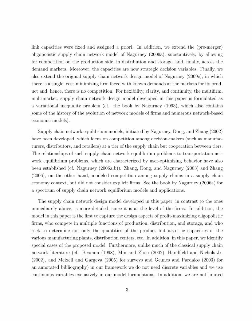
Figure 1: The Initial Supply Chain Network Topology of the Oligopoly
(see Nagurney, Takayama, and Zhang (1995) and Nagurney and Zhang (1996a)), dynamic
network oligopolies (cf. Nagurney, Dupuis, and Zhang (1994)), and dynamic traffic network
equilibrium problems (see, e.g., Zhang and Nagurney (1997) and Yang and Zhang (2009)).
In Section 4, we provide numerical examples. In Section 5, we summarize the results in
this paper and give suggestions for future research.
2. The Supply Chain Network Design Model
In this Section, we develop the supply chain network design model with profit-maximizing
firms and identify several special cases. We consider a finite number of I firms, with a
typical firm denoted by i, who are involved in the production, storage, and distribution of a
homogeneous product and who compete noncooperatively in an oligopolistic manner.
We assume that each firm is represented as an initial network of its economic activities
(cf. Figure 1). Each firm seeks to determine its optimal link capacities and product quan-
tities by using Figure 1 as a schematic. Each firm i; i = 1, . . . , I, hence, is considering
niM manufacturing facilities/plants; ni
D distribution centers, and serves the same nR retail
5

outlets/demand markets. Let L0i denote the set of directed links representing the economic
activities associated with firm i; i = 1, . . . , I and let nL0i
denote the number of links in L0i
with nL0 denoting the total number of links in the initial network L0, where L0 ≡ ∪i=1,IL0i .
Let G0 = [N0, L0] denote the graph consisting of the set of nodes N0 and the set of links L0
in Figure 1. Once the supply chain design problem is solved, those links with zero optimal
capacities (and, hence, also zero product flows) can, in effect, be eliminated from the final
supply chain network design topology.
The links from the top-tiered nodes i; i = 1, . . . , I, representing the respective firm, in
Figure 1 are connected to the manufacturing nodes of the respective firm i, which are denoted,
respectively, by: M i1, . . . ,M
ini
M, and these links represent the manufacturing links. The links
from the manufacturing nodes, in turn, are connected to the distribution center nodes of
each firm i; i = 1, . . . , I, which are denoted by Di1,1, . . . , D
inD
i,1. These links correspond
to the shipment links between the manufacturing plants and the distribution centers where
the product is stored. The links joining nodes Di1,1, . . . , D
ini
D,1 with nodes Di1,2, . . . , D
ini
D,2 for
i = 1, . . . , I correspond to the storage links. Finally, there are possible shipment links joining
the nodes Di1,2, . . . , D
ini
D,2 for i = 1, . . . , I with the demand market nodes: R1, . . . , RnR.
We emphasize that the network topology in Figure 1, which corresponds to G0 is given
here for descriptive purposes and, for definiteness. In fact, the model, described fully below,
can handle any prospective supply chain network topology provided that there is a top-tiered
node to represent each firm and bottom-tiered nodes to represent the demand markets with
a sequence of directed links, corresponding to at least one path, joining each top-tiered node
with each bottom-tiered node. The solution of the complete model will identify which links
have positive capacities and, hence, should be retained in the final supply chain network
design.
We assume that associated with each link (cf. Figure 1) of the network corresponding
to each firm i; i = 1, . . . , I is a total cost associated with operating the link over the time
horizon under consideration. We also assume that there is a total design cost associated
with each link. We denote, without any loss in generality, the links by a, b, etc., the total
operational cost on a link a by ca and the total design cost by πa, for all links a ∈ L0.
Let dRkdenote the demand for the product at demand market Rk; k = 1, . . . , nR. Let xp
6

denote the nonnegative flow of the product on path p joining (origin) node i; i = 1, . . . , I
with a (destination) demand market node. Then the following conservation of flow equations
must hold: ∑p∈P 0
Rk
xp = dRk, k = 1, . . . , nR, (1)
where P 0Rk
denotes the set of paths connecting the (origin) nodes i; i = 1, . . . , I with (des-
tination) demand market Rk. In particular, we have that P 0Rk
= ∪i=1,...,IP0Ri
k, where P 0
Rik
denotes the set of paths from origin node i to demand market k as in Figure 1.
According to (1), the demand at each demand market must be equal to the sum of the
product flows from all firms to that demand market.
We assume that there is a demand price function associated with the product at each
demand market. We denote the demand price at demand market Rk by ρRkand we assume,
as given, the demand price functions:
ρRk= ρRk
(d), k = 1, . . . , nR, (2)
where d is the nR-dimensional vector of demands at the demand markets. We assume that all
vectors in this paper are column vectors. Note that we consider the general situation where
the price for the product at a particular demand market may, in general, depend upon
the demand for the product at the other demand markets. We assume that the demand
price functions are continuous, continuously differentiable, and monotone decreasing. Note
that the consumers at each demand market are indifferent as to which firm produced the
homogeneous product.
In addition, we let fa denote the flow of the product on link a. Hence, we must also have
the following conservation of flow equations satisfied:
fa =∑
p∈P 0
xpδap, ∀a ∈ L0, (3)
where δap = 1 if link a is contained in path p and δap = 0, otherwise. Here P 0 denotes the
set of all paths in Figure 1, that is, P 0 = ∪k=1,...,nRP 0
Rk. There are nP 0 paths in the network
in Figure 1. We use P 0i to denote the set of all paths from firm i to all the demand markets
for i = 1, . . . , I. There are nP 0i
paths from the firm i node to the demand markets.
7

Of course, we also have that the path flows must be nonnegative, that is,
xp ≥ 0, ∀p ∈ P 0. (4)
Let ua, a ∈ L0, denote the design capacity of link a, where we must have that
fa ≤ ua, ∀a ∈ L0, (5)
or, in view of (3) ∑p∈P 0
xpδap ≤ ua, ∀a ∈ L0. (6)
In other words, the product flow on each link is bounded by the capacity (which is a
strategic decision variable) on the link.
The total operational cost on a link, be it a manufacturing/production link, a ship-
ment/distribution link, or a storage link is assumed, in general, to be a function of the flows
of the product on all the links, that is,
ca = ca(f), ∀a ∈ L0, (7)
where f is the vector of all the link flows.
In addition, we assume that the total design cost associated with each link is a function
of the design capacity on the link, that is,
πa = πa(ua), ∀a ∈ L0. (8)
Let Xi denote the vector of strategy variables associated with firm i; i = 1, . . . , I, where
Xi is the vector of path flows associated with firm i, and the vector of link capacities, that
is, Xi ≡ {{{xp}|p ∈ P 0i }; {{ua}|a ∈ L0
i }} ∈ Rn
P0i+n
L0i
+ . X is then the vector of all the firms’
strategies, that is, X ≡ {{Xi}|i = 1, . . . , I}}.
The profit function Ui of firm i; i = 1, . . . , I, is the difference between the firm’s revenue
and its total costs, that is,
Ui =nR∑k=1
ρRk(d)
∑p∈P 0
Rik
xp −∑
a∈L0i
ca(f)−∑
a∈L0i
πa(ua). (9)
8

In view of (1) – (9), we may write:
U = U(X), (10)
where U is the I-dimensional vector of the firms’ profits.
We now consider the oligopolistic market mechanism in which the I firms select their
supply chain network link capacities and product path flows in a noncooperative manner,
each one trying to maximize its own profit. We seek to determine a path flow and capacity
pattern X for which the I firms will be in a state of equilibrium as defined below.
Definition 1: Supply Chain Network Design Cournot-Nash Equilibrium
A path flow and design capacity pattern X∗ ∈ K0 =∏I
i=1K0i is said to constitute a supply
chain network design Cournot-Nash equilibrium if for each firm i; i = 1, . . . , I:
Ui(X∗i , X∗
i ) ≥ Ui(Xi, X∗i ), ∀Xi ∈ K0
i , (11)
where X∗i ≡ (X∗
1 , . . . , X∗i−1, X
∗i+1, . . . , X
∗I ) and K0
i ≡ {Xi|Xi ∈ Rn
P0i+n
L0i
+ , and (6) is satisfied}.
Note that, according to (11), a supply chain network design Cournot-Nash equilibrium
has been established if no firm can increase its profits unilaterally.
The variational inequality formulation of the Cournot-Nash (Cournot (1838), Nash (1950,
1951)) supply chain network design problem satisfying Definition 1 is given in the following
theorem.
Theorem 1
Assume that for each firm i; i = 1, . . . , I, the profit function Ui(X) is concave with respect
to the variables in Xi, and is continuously differentiable. Then X∗ ∈ K0 is a supply chain
network design Cournot-Nash equilibrium according to Definition 1 if and only if it satisfies
the variational inequality:
−I∑
i=1
〈∇XiUi(X
∗)T , Xi −X∗i 〉 ≥ 0, ∀X ∈ K0, (12)
where 〈·, ·〉 denotes the inner product in the corresponding Euclidean space and ∇XiUi(X)
denotes the gradient of Ui(X) with respect to Xi. The solution of variational inequality (12)
9

is equivalent to the solution of variational inequality: determine (x∗, u∗, λ∗) ∈ K1 satisfying:
I∑i=1
nR∑k=1
∑p∈P 0
Rik
∂Cp(x∗)
∂xp
+∑
a∈L0
λ∗aδap − ρRk(x∗)−
nR∑l=1
∂ρRl(x∗)
∂dRk
∑p∈P 0
Rik
x∗p
× [xp − x∗p]
+∑
a∈L0
[∂πa(u
∗a)
∂ua
− λ∗a
]× [ua − u∗a]
+∑
a∈L0
u∗a −∑
p∈P 0
x∗pδap
× [λa − λ∗a] ≥ 0, ∀(x, u, λ) ∈ K1, (13)
where K1 ≡ {(x, u, λ)|x ∈ RnP0
+ ; u ∈ RnL0
+ ; λ ∈ RnL0
+ } and ∂Cp(x)∂xp
≡ ∑b∈L0
i
∑a∈L0
i
∂cb(f)∂fa
δap for
paths p ∈ P 0i ; i = 1, . . . , I.
Proof: Variational inequality (12) follows directly from Gabay and Moulin (1980); see also
Dafermos and Nagurney (1987). Here we have also utilized the fact that the demand price
functions (2) can be reexpressed in light of (1) directly as a function of path flows as can
the total operational cost functions (7). Variational inequality (13) follows, in turn, from
Bertsekas and Tsitsiklis (1989) with notice that λ∗ corresponds to the vector of optimal
Lagrange multipliers associated with constraints (6).
Variational inequality (13) can be put into standard form as below: determine X∗ ∈ Ksuch that
〈F (X∗)T , X −X∗〉 ≥ 0, ∀X ∈ K, (14)
where K is closed and convex and F (X) is a continuous function from K to Rn. Indeed,
we can define K ≡ K1 and let F (X) be the vector with nP 0 + 2nL0 components given by
the specific terms preceding the first multiplication sign in (13), the second in (13), and the
third in (13).
It is interesting to relate this supply chain network design oligopoly model to the spatial
oligopoly model proposed by Dafermos and Nagurney (1987), which is done in the following
corollary.
10

Corollary 1
Assume that there are I firms in the supply chain network design oligopoly model and that
each firm is considering a single manufacturing plant and a single distribution center. As-
sume also that the distribution costs from each manufacturing plant to the distribution center
and the storage costs are all equal to zero. Then the resulting model is a generalization of
the spatial oligopoly model of Dafermos and Nagurney (1987) with the inclusion of design
capacities as strategic variables and whose underlying initial network structure is given in
Figure 2.
Proof: Follows from Dafermos and Nagurney (1987) and Nagurney (1993).
Hence, the above supply chain network design oligopoly model, as a spcial case, provides
us with an extension to the spatial oligopoly model of Dafermos and Nagurney (1987). It
is also interesting to note that in the new supply chain network design oligopoly model
there is competition on the supply and distribution sides as well as on the demand side,
since the cost functions associated with production, with distribution, and with storage
may, in general, depend upon not only the flows of the particular firm but, rather, on
the flows of all the firms. In Dafermos and Nagurney (1987) and in Nagurney (1993) the
network structure of the spatial oligopoly problem is depicted as a bipartite graph with
the manufacturing assumed to take place at the manufacturing/production nodes. In the
supply chain network design formalism here, we associate the production with links, and
the outputs are, hence, the link flows, and, thus, Figure 2 makes this explicit. Dafermos
and Nagurney (1987) also establish the relationships between spatial Cournot oligopolies
and perfectly competitive spatial price equilibrium problems (cf. Dafermos and Nagurney
(1987)). Nagurney, Dupuis, and Zhang (1994), in turn, developed a dynamic version of
the model of Dafermos and Nagurney (1987) using projected dynamical systems theory (see
also Nagurney and Zhang (1996b)). Of course, those models, unlike the ones proposed in
this paper, did not have the capacity design variables in their formulations. Our framework
allows for such a generalization and, as we will see in the following sections, without much
additional cost in terms of computations and problem solution.
It is also interesting to relate the supply chain network oligopoly model to the classi-
11

m m m
m m m
1 2 · · · nR
M11 M2
1 · · ·M I1
���������
AAAAAAAAU
aaaaaaaaaaaaaaaaaaa
���
��
��
��
��+
���������
QQQQQQQQQQQ
AAAAAAAAU
���
���
��
���+
!!!!!!!!!!!!!!!!!!!
m m m? ? ?
1 2 I
Figure 2: The Initial Network Topology of the Spatial Oligopoly Design Problem
cal Cournot (1838) oligopoly model in quantity variables, which has been formulated as a
variational inequality problem by Gabay and Moulin (1980) and has been studied by both
economists and operations researchers (cf. Murphy, Sherali, and Soyster (1982), Flam and
Ben-Israel (1990), Nagurney (1993), and the references therein). Indeed, we have the follow-
ing corollary, the proof of which is immediate.
Corollary 2
Assume that there is a single manufacturing plant associated with each firm in the above
supply chain network design model and a single distribution center. Assume also that there
is a single demand market. Assume that the manufacturing cost of each firm depends only
upon its own output. Then, if the storage and distribution cost functions are all identically
equal to zero the above design model collapses to an extension of the classical oligopoly model
in quantity variables and with capacity design variables. Furthermore, if I = 2, one then
obtains a generalization of the classical duopoly model.
The initial network structure for the classical oligopoly problem (see also Nagurney (1993,
2009a)) is depicted in Figure 3. The classical model is an aspatial model since there are no
explicit transportation/transaction costs between the firms/manufacturers and the demand
12

mR1
@@@R
���
D11,2
m · · · mD1nI
D,2
? ?
D11,1
m · · · mD1nI
D,1
? ?
M I1
m · · · mM1nI
M
? ?
m1 · · · mIFirm 1 Firm I
m
m· · ·1 2 I
HHj���
R1
⇒
Figure 3: The Initial Network Topology of the “Classical” Oligopoly Design Problem
market.
Existence results for both spatial and aspatial oligopoly problems can be found in Nagur-
ney and Zhang (1996b) and the references therein. Typically, either strong monotonicity or
coercivity conditions are imposed on the relevant functions in order to guarantee existence
of a Cournot-Nash equilibrium in such applications.
We emphasize that with the variational inequality formulation of the competitive supply
chain network design problem, as given above, we can now:
1. consider problems in which there are nonlinearities as well as asymmetries in the under-
lying functions, for which an optimization formulation would no longer suffice and
2. obtain further insights into competitive oligopolistic equilibrium problems that character-
ize a variety of industries with the generalization of the inclusion of explicit design variables.
Moreover, as is well-known, intuition in the case of equilibrium problems, as opposed
to optimization problems, may be easily confounded (as in the Braess paradox; see Braess
(1968) and Braess, Nagurney, and Wakolbinger (2005)). Hence, an oligopolistic supply chain
13

network design framework, which allows for the computation of solutions, can allow firms to
investigate their optimal strategies in the presence of competition.
3. The Algorithm
In this Section, we recall the Euler method, which is induced by the general iterative
scheme of Dupuis and Nagurney (1993). Its realization for the solution of supply chain
network design problems governed by variational inequality (13) yields subproblems that
can be solved explicitly and in closed form.
Specifically, recall that at an iteration τ of the Euler method (see also Nagurney and
Zhang (1996b)) one computes:
Xτ+1 = PK(Xτ − aτF (Xτ )), (15)
where PK is the projection on the feasible set K and F is the function that enters the
variational inequality problem: determine X∗ ∈ K such that
〈F (X∗)T , X −X∗〉 ≥ 0, ∀X ∈ K, (16)
where 〈·, ·〉 is the inner product in n-dimensional Euclidean space, X ∈ Rn, and F (X) is an
n-dimensional function from K to Rn, with F (X) being continuous (see also (14)).
As shown in Dupuis and Nagurney (1993); see also Nagurney and Zhang (1996b), for
convergence of the general iterative scheme, which induces the Euler method, among other
methods, the sequence {aτ} must satisfy:∑∞
τ=0 aτ = ∞, aτ > 0, aτ → 0, as τ → ∞.
Specific conditions for convergence of this scheme can be found for a variety of network-
based problems, similar to those constructed here, in Nagurney and Zhang (1996b) and the
references therein.
Explicit Formulae for the Euler Method Applied to the Supply Chain Network
Design Variational Inequality (13)
The elegance of this procedure for the computation of solutions to the supply chain network
design problem modeled in Section 2 can be seen in the following explicit formulae. Indeed,
(15) for the supply chain design network oligopoly problem governed by variational inequality
14

problem (13) yields the following closed form expressions for the product path flows, the
design capacities, and the Lagrange multipliers, respectively:
xτ+1p = max{0, xτ
p+aτ (ρRk(xτ )−
nR∑l=1
∂ρl(xτ )
∂dRk
∑p∈P 0
Rik
xτp−
∂Cp(xτ )
∂xp
−∑
a∈L0
λτaδap)}, ∀i,∀k,∀p ∈ P 0
Rik;
(17)
uτ+1a = max{0, uτ
a + aτ (λτa −
∂πa(uτa)
∂ua
)}, ∀a ∈ L0; (18)
λτ+1a = max{0, λτ
a + aτ (∑
p∈P 0
xτpδap − uτ
a)}, ∀a ∈ L0. (19)
In the next Section, we solve supply chain network oligopoly design problems using this
algorithmic scheme.
4. Numerical Examples
In this Section, we present numerical supply chain network design oligopoly examples of
increasing complexity. We implemented the Euler method, as discussed in Section 3. The
algorithm code were implemented in FORTRAN and the system used for the computations
was a Unix system at the University of Massachusetts Amherst. The convergence tolerance
was: |Xτ+1 − Xτ | ≤ 10−6 for all the examples. The sequence {aτ} used (cf. (15)) was:
.1{1, 12, 1
2, 1
3, 1
3, 1
3, . . . , }. We initialized the Euler method as follows. We set the demand for
the product at 100 for each demand market and equally distributed the demand among all
the paths. The initial link design capacities as well as the initial Lagrange multipliers were
all set to zero.
Example 1
Example 1 consisted of four firms with the prospective supply chain network topology as
in Figure 4. Each firm was considering a single manufacturing plant, a single distribution
center, and a single demand market.
For simplicity, we let all the total operational cost functions on the links be equal and
given by:
ca(f) = 2f 2a + fa, ∀a ∈ L0
i ; i = 1, 2, 3, 4. (20)
15

����R1
���� ���� ���� ����D1
1,2 D21,2 D3
1,2 D41,2
SSSSw
����/
���� ���� ���� ����D1
1,1 D21,1 D3
1,1 D41,1
? ? ? ?
���� ���� ���� ����M1
1 M21 M3
1 M41
? ? ? ?
���� ���� ���� ����1 2 3 4
? ? ? ?
The Firms
Figure 4: The Initial Network Topology for Examples 1 and 2
The total design cost functions on all the links were:
πa(ua) = 5u2a + ua, ∀a ∈ L0
i ; i = 1, 2, 3, 4. (21)
The demand price function at the single demand market was:
ρR1(d) = −dR1 + 200. (22)
We denoted the paths by p1, p2, p3, and p4 corresponding to firm 1 through firm 4,
respectively, with each path originating in its top-most firm node and ending in the demand
market node (cf. Figure 4).
The Euler method converged to the equilibrium solution:
x∗p1= x∗p2
= x∗p3= x∗p4
= 3.15,
16

u∗a = 3.15,∀a ∈ L0, f ∗a = 3.15,∀a ∈ L0,
λ∗a = 32.46,∀a ∈ L0.
Hence, the supply chain network design, since all links had positive capacities (as well as
positive flows), had the topology as in Figure 4.
The demand was 12.60 and the demand market price was ρR1 = 187.40. Each firm earned
a profit of 287.88.
Example 2
Example 2 was constructed from Example 1 and had the same data except that the demand
price at the demand market was greatly reduced to:
ρR1(d) = −dR1 + 5. (23)
The Euler method converged to the solution with all path flows, link flows, and design
capacities equal to 0.00 with the Lagrange multipliers all equal to 1.05. Hence, not one of
the firms enters into this market and none of these firms produces the product. Therefore,
the final supply chain network design is essentially the null set.
Example 3
Example 3 had the initial supply chain network topology as in Figure 5, where we also define
the links. Specifically, there were two firms considering two manufacturing plants each, two
distribution centers each, and considering serving a single demand market.
The total cost data, along with the computed link flows, capacities, and Lagrange multi-
pliers, are reported in Table 1. This example represents the following scenario. Let the first
firm be located in the US, for example, where there are higher manufacturing costs and also
higher costs associated with both constructing the manufacturing plants and the distribution
centers; see: c1, c5, and π1, π5. The second firm, on the other hand, is located outside the
US where there are lower manufacturing costs and storage costs as well as associated design
costs for the facilities; see c11, c15, and π11, π15. However, the demand market is in the US
17
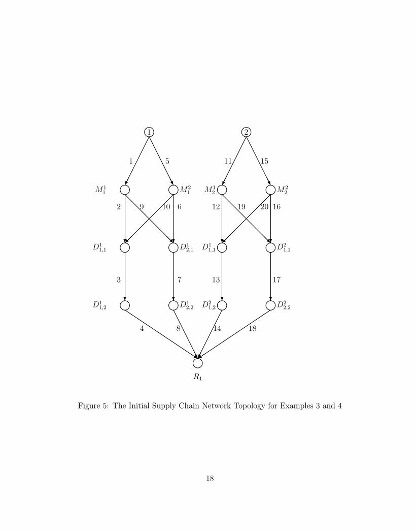
m1 m2���������
AAAAAAAAU
���������
AAAAAAAAU
1 5 11 15
M11 M2
1 M12 M2
2m m m m
?
@@@@@@@@R?
��
��
��
�� ?
@@@@@@@@R
���
��
��� ?
2
3 7 13 17
9 10 6 12 19 20 16
D11,1 D1
2,1 D11,1 D2
1,1m m m m
? ? ? ?D1
1,2 D12,2 D2
1,2 D22,2
m m m m�
���
��
���
��+
���������
AAAAAAAAU
QQQQQQQQQQQsmR1
4 8 14 18
Figure 5: The Initial Supply Chain Network Topology for Examples 3 and 4
18

Table 1: Total Cost Functions and Solution for Example 3
Link a ca(f) πa(ua) f ∗a u∗a λ∗a1 2f 2
1 + 2f1 5u21 + u1 7.28 7.28 74.05
2 f 22 + 2f2 .5u2
2 + u2 3.98 3.98 4.983 2.5f 2
3 + f3 5u23 + 2u3 7.54 7.54 76.23
4 f 24 + f4 .5u2
4 + u4 7.54 7.54 8.545 3f 2
5 + 2f5 6u25 + u5 5.73 5.73 70.05
6 .5f 26 + f6 .5u2
6 + u6 2.17 2.17 3.177 1.5f 2
7 + f7 10u27 + u7 5.47 5.47 110.07
8 f 28 + f8 .5u2
8 + u8 5.47 5.47 6.489 .5f 2
9 + f9 .5u29 + u9 3.30 3.30 4.30
10 f 210 + f10 .5u2
10 + u10 3.56 3.56 4.5611 .5f 2
11 + f11 4u211 + u11 7.15 7.15 58.23
12 f 212 + f12 .5u2
12 + u12 2.98 2.98 3.9813 .5f 2
13 + f13 2.5u213 + u13 7.14 7.14 36.72
14 4f 214 + f14 5u2
14 + 5u14 7.14 7.14 76.1915 f 2
15 + f15 3u215 + u15 8.12 8.12 49.76
16 f 216 + f16 .5u2
16 + u16 3.96 3.96 4.9617 .5f 2
17 + f17 2.5u217 + u17 8.13 8.13 41.66
18 3.5f 218 + f18 4u2
18 + 2u18 8.13 8.13 66.8919 f 2
19 + f19 .5u219 + u19 4.17 4.17 5.17
20 .5f 220 + f20 .5u2
20 + u20 4.16 4.16 5.16
and, hence, the second firm faces higher transportation costs to deliver the product to the
demand market, as can be seen from the function data in Table 1; see c14 and c18 versus c4
and c8.
The demand price function was:
ρR1(d) = −dR1 + 300. (24)
For completeness, we also provide the computed equilibrium path flows. There were four
paths for each firm and we label the paths as follows (please refer to Figure 5): for firm 1:
p1 = (1, 2, 3, 4), p2 = (1, 9, 7, 8), p3 = (5, 6, 7, 8), p4 = (5, 10, 3, 4),
19

for firm 2:
p5 = (11, 12, 13, 14), p6 = (11, 19, 17, 18), p7 = (15, 16, 17, 18), p8 = (15, 20, 13, 14).
The computed equilibrium path flow pattern was:
x∗p1= 3.98, x∗p2
= 3.30, x∗p3= 2.17, x∗p4
= 3.56,
x∗p5= 2.98, x∗p6
= 4.17, x∗p7= 3.96, x∗p8
= 4.16.
Example 4
Example 4 also had the initial supply chain network topology as in Figure 5. Example 4 had
the same data as Example 3 except we reduced the capacity design costs associated with the
shipment links from the second firm to the demand market as in Table 2; see π14 and π18.
The total cost data, along with the computed link flows, capacities, and Lagrange multi-
pliers, are reported in Table 2.
The demand price was: 267.47 and the total profit earned by both firms was: 4,493.29.
For completeness, we also provide the computed equilibrium path flows, which were:
x∗p1= 3.92, x∗p2
= 3.25, x∗p3= 2.13, x∗p4
= 3.51,
x∗p5= 4.04, x∗p6
= 5.19, x∗p7= 4.89, x∗p8
= 5.60.
One can see that the second firm manufactured a greater volume of the product than
the first firm and provided more of the product to the consumers at the demand market.
Hence, in this example the firm that had lower overseas costs was more competitive once the
shipment costs were further reduced.
Note that the final supply chain network topology under the optimal design for Example
4 remained as in Figure 5.
20

Table 2: Total Cost Functions and Solution for Example 4
Link a ca(f) πa(ua) f ∗a u∗a λ∗a1 2f 2
1 + 2f1 5u21 + u1 7.17 7.17 72.87
2 f 22 + 2f2 .5u2
2 + u2 3.92 3.92 4.923 2.5f 2
3 + f3 5u23 + 2u3 7.42 7.42 75.01
4 f 24 + f4 .5u2
4 + u4 7.42 7.42 8.425 3f 2
5 + 2f5 6u25 + u5 5.64 5.64 68.93
6 .5f 26 + f6 .5u2
6 + u6 2.13 2.13 3.147 1.5f 2
7 + f7 10u27 + u7 5.39 5.39 108.30
8 f 28 + f8 .5u2
8 + u8 5.39 5.39 6.399 .5f 2
9 + f9 .5u29 + u9 3.25 3.25 4.25
10 f 210 + f10 .5u2
10 + u10 3.51 3.51 4.5011 .5f 2
11 + f11 4u211 + u11 9.23 9.23 74.74
12 f 212 + f12 .5u2
12 + u12 4.04 4.04 5.0413 .5f 2
13 + f13 2.5u213 + u13 9.64 9.64 49.24
14 4f 214 + f14 .5u2
14 + u14 9.64 9.64 10.6415 f 2
15 + f15 3u215 + u15 10.49 10.49 63.90
16 f 216 + f16 .5u2
16 + u16 4.89 4.89 5.8917 .5f 2
17 + f17 2.5u217 + u17 10.08 10.08 51.44
18 3.5f 218 + f18 .5u2
18 + u18 10.08 10.08 11.0819 f 2
19 + f19 .5u219 + u19 5.19 5.19 6.19
20 .5f 220 + f20 .5u2
20 + u20 5.60 5.60 6.60
21

Example 5
Example 5 had the same data as Example 4 but now we added a second demand market
with the initial supply chain network topology being as depicted in Figure 6. The links are
labeled on that figure. We assumed that the second demand market was located in the US
with the shipment costs set to reflect this scenario. The demand price function for the first
demand market remained as in Examples 3 and 4. The demand price function for the new
demand market was:
ρR2(d) = −2dR2 + 500. (25)
The remainder of the input data and the computed solution are given in Table 3.
For completeness, we also provide the computed path flows. We retained the numbering
and the definitions of the first eight paths for the first demand market as in Examples 3 and
4 (but associated now with Figure 6). The new paths for the first firm to the second demand
market are defined as:
p9 = (1, 2, 3, 21), p10 = (1, 9, 7, 22), p11 = (5, 6, 7, 22), p12 = (5, 10, 3, 21),
and for the second firm to the second demand market as:
p13 = (11, 12, 13, 23), p14 = (11, 19, 17, 24), p15 = (15, 16, 17, 24), p16 = (15, 20, 13, 23).
The computed path flow solution follows:
x∗p1= 0.00, x∗p2
= 0.00, x∗p3= 0.00, x∗p4
= 0.00,
x∗p5= 0.49, x∗p6
= 0.72, x∗p7= 0.79, x∗p8
= 1.84.
x∗p9= 5.75, x∗p10
= 4.54, x∗p11= 3.04, x∗p12
= 5.08,
x∗p13= 6.49, x∗p14
= 8.15, x∗p15= 7.55, x∗p16
= 7.84.
It is very interesting to note that the first firm no longer provides any of the product to
the first demand market and, in fact, all its associated path flows to the first demand market
are now equal to zero as are the link flows on links 4 and 8. In addition, the associated
design capacities on links 4 and 8 are also equal to zero. Thus, for Example 5, the optimal
supply chain network design is as given in Figure 7.
22

Table 3: Total Cost Functions and Solution for Example 5
Link a ca(f) πa(ua) f ∗a u∗a λ∗a1 2f 2
1 + 2f1 5u21 + u1 10.29 10.29 104.12
2 f 22 + 2f2 .5u2
2 + u2 5.75 5.75 6.753 2.5f 2
3 + f3 5u23 + 2u3 10.83 10.83 109.09
4 f 24 + f4 .5u2
4 + u4 0.00 0.00 0.045 3f 2
5 + 2f5 6u25 + u5 8.12 8.12 98.65
6 .5f 26 + f6 .5u2
6 + u6 3.04 3.04 4.047 1.5f 2
7 + f7 10u27 + u7 7.58 7.58 151.81
8 f 28 + f8 .5u2
8 + u8 0.00 0.00 0.569 .5f 2
9 + f9 .5u29 + u9 4.54 4.54 5.54
10 f 210 + f10 .5u2
10 + u10 5.08 5.08 6.0811 .5f 2
11 + f11 4u211 + u11 15.84 15.84 127.61
12 f 212 + f12 .5u2
12 + u12 6.98 6.98 7.9813 .5f 2
13 + f13 2.5u213 + u13 16.66 16.66 84.34
14 4f 214 + f14 .5u2
14 + u14 2.33 2.33 3.3315 f 2
15 + f15 3u215 + u15 18.02 18.02 109.00
16 f 216 + f16 .5u2
16 + u16 8.34 8.34 9.3417 .5f 2
17 + f17 2.5u217 + u17 17.20 17.20 87.04
18 3.5f 218 + f18 .5u2
18 + u18 1.51 1.51 2.5119 f 2
19 + f19 .5u219 + u19 8.86 8.86 9.86
20 .5f 220 + f20 .5u2
20 + u20 9.68 9.68 10.6821 .5f 2
21 + f21 2.5u221 + f21 10.83 10.83 23.66
22 f 222 + f22 .5u2
22 + f22 7.58 7.58 17.1623 2f 2
23 + f23 .5u223 + f23 14.33 14.33 15.33
24 1.5f 224 + f22 .5u2
24 + f24 15.70 15.70 16.69
23

m1 m2���������
AAAAAAAAU
���������
AAAAAAAAU
1 5 11 15
M11 M2
1 M12 M2
2m m m m
?
@@@@@@@@R?
��
��
��
�� ?
@@@@@@@@R
���
��
��� ?
2
3 7 13 17
24
9 10 6 12 19 20 16
D11,1 D1
2,1 D11,1 D2
1,1m m m m
? ? ? ?D1
1,2 D12,2 D2
1,2 D22,2
m m m m
?
���
���
��
���+
@@@@@@@@R
���������
HHHHHHH
HHHHHHHH
AAAAAAAAU
PPPPPPPPPPPPPPPPPPPPPP
QQQQQQQQQQQsm mR1
4
21 22 23
8 14 18
R2
Figure 6: The Initial Supply Chain Network Topology for Example 5
24

m1 m2���������
AAAAAAAAU
���������
AAAAAAAAU
1 5 11 15
M11 M2
1 M12 M2
2m m m m
?
@@@@@@@@R?
��
��
��
�� ?
@@@@@@@@R
���
��
��� ?
2
3 7 13 17
24
9 10 6 12 19 20 16
D11,1 D1
2,1 D11,1 D2
1,1m m m m
? ? ? ?D1
1,2 D12,2 D2
1,2 D22,2
m m m m
?
���
���
��
���+
@@@@@@@@R
���������
HHHHHHH
HHHHHHHH
PPPPPPPPPPPPPPPPPPPPPPm mR1
21 22 23
14 18
R2
Figure 7: The Optimal Supply Chain Network Design for Example 5
25

5. Summary and Conclusions
In this paper, we developed a multimarket supply chain network design model in an
oligopolistic setting. The firms select not only their optimal product flows but also the
capacities associated with the various supply chain activities of production/manufacturing,
storage, and distribution/shipment. We formulated the supply chain network design problem
as a variational inequality problem and then proposed an algorithm, which fully exploits the
underlying structure of these network problems, and yields closed form expressions at each
iterative step.
The network formalism proposed here, which captures competition on the production,
distribution, as well as demand market dimensions, enables the investigation of economic
issues surrounding supply chain network design. In addition, it allows for the identification
(and generalization) of special cases of oligopolistic market equilibrium problems, spatial,
as well as aspatial, through the underlying network structure, that have appeared in the
literature. Furthermore, the network structure allows one to visualize graphically the pro-
posed supply chain network topology and the final optimal/equilibrium design. Importantly,
this paper illustrates the power of computational methodologies to explore issues regarding
competing firms and network design. Moreover, we demonstrate that such problems can be
formulated and solved without using discrete variables but, rather only continuous variables.
The research in this paper can be extended in several directions. One can construct
multiproduct versions of the oligopolistic supply chain network design model developed here,
and one can also consider more explicitly international/global issues with the incorporation
of exchange rates and risk. It would also be worthwhile to formulate supply chain network
redesign oligopolistic models. Obviously, further computational experimentation as well as
theoretical developments and empirical applications would also be of value, but we leave
such research questions/problems for the future.
Acknowledgments
This research was supported by the John F. Smith Memorial Fund at the Isenberg School
of Management. This support is gratefully acknowledged.
26

The author also acknowledges the helpful comments and suggestions of two anonymous
reviewers and the Editor on an earlier version of this paper.
References
Beamon, B. M., 1998. Supply chain design and analysis: Models and methods. International
Journal of Production Economics 55, 281-294.
Bertsekas, D. P., Tsitsiklis, J. N., 1989. Parallel and Distributed Computation. Prentice-
Hall, Englewood Cliffs, New Jersey.
Braess, D., 1968. Uber ein paradoxon aus der verkehrsplanung. Unternehmenforschung 12,
258-268.
Braess, D., Nagurney, A., Wakolbinger, T., 2005. On a paradox of traffic planning, transla-
tion of the 1968 article by Braess. Transportation Science 39, 446-450.
Brown, G., Keegan, J., Vigus, B., Wood, K., 2001. The Kellogg company optimizes produc-
tion, inventory and distribution. Interfaces 31, 1-15.
Cournot, A. A., 1838. Researches into the Mathematical Principles of the Theory of Wealth,
English translation, MacMillan, London, England, 1897.
Dafermos, S., Nagurney, A. 1987. Oligopolistic and competitive behavior of spatially sepa-
rated markets. Regional Science and Urban Economics 17, 245-254.
Dupuis, P., Nagurney, A., 1993. Dynamical systems and variational inequalities. Annals of
Operations Research 44, 9-42.
Flam, S. P., Ben-Israel, A., 1990. A continuous approach to oligopolistic market equilibrium
Operations Research 38, 1045-1051.
Gabay, D., Moulin, H., 1980. On the uniqueness and stability of Nash equilibria in noncoop-
erative games. In: Bensoussan, A., Kleindorfer, P., Tapiero, C. S. (Eds), Applied Stochastic
Control of Econometrics and Management Science, North-Holland, Amsterdam, The Nether-
lands, pp. 271-294.
27

Geunes, J., Pardalos, P. M., 2003. Network optimization in supply chain management and
financial engineering: An annotated bibliography. Networks, 42, 66-84.
Handfield, R. B., Nichols Jr., E. L., 2002. Supply Chain Redesign: Transforming Supply
Chains into Integrated Value Systems. Financial Times Prentice Hall, Upper Saddle River,
New Jersey.
Meixell, M. J., Gargeya, V. B., 2005. Global supply chain design: A literature review and
critique. Transportation Research E, 41, 531-550.
Min, H., Zhou, G., 2002. Supply chain modeling: past, present, future. Computers and
Industrial Engineering 43, 231-249.
Murphy, F. H., Sherali, H. D., Soyster, A. L., 1982. A mathematical programming approach
for determining oligopolistic market equilibrium. Mathematical Programming 24, 92-106.
Nagurney, A., 1993. Network Economics: A Variational Inequality Approach. Kluwer Aca-
demic Publishers, Dordrecht, The Netherlands.
Nagurney, A. 2006a. Supply Chain Network Economics: Dynamics of Prices, Flows and
Profits. Edward Elgar Publishing, Cheltenham, England.
Nagurney, A. 2006b. On the relationship between supply chain and transportation network
equilibria: A supernetwork equivalence with computations. Transportation Research E 42,
293-316.
Nagurney, A., 2009a. Formulation and analysis of horizontal mergers among oligopolistic
firms with insights into the merger paradox: A supply chain network perspective. Compu-
tational Management Science, in press.
Nagurney, A., 2009b. A system-optimization perspective for supply chain network integra-
tion: The horizontal merger case. Transportation Research E 45, 1-15.
Nagurney, A., 2009c. Optimal supply chain network design at minimal total cost and de-
mand satisfaction. Isenberg School of Management, University of Massachusetts, Amherst,
28

Massachusetts.
Nagurney, A., Dong, J., Zhang, D., 2002. A supply chain network equilibrium model. Trans-
portation Research E 38, 281-303.
Nagurney, A., Dupuis, P., Zhang, D., 1994, A dynamical systems approach for network
oligopolies and variational inequalities. Annals of Operations Research 28, 263-293.
Nagurney, A., Qiang, Q., 2009. Fragile Networks: Identifying Vulnerabilities and Synergies
in an Uncertain World. John Wiley & Sons, Hoboken, New Jersey.
Nagurney, A., Takayama, T., Zhang, D., 1995. Massively parallel computation of spatial
price equilibrium problems as dynamical systems. Journal of Economic Dynamics and Con-
trol 18, 3-37.
Nagurney, A., Woolley, T., 2009. Environmental and cost synergy in supply chain net-
work integration in mergers and acquisitions. In: Ehrgott, M., Naujoks, B., Stewart, T. J.,
Wallenius, J. (Eds), Multiple Criteria Decision Making for Sustainable Energy and Trans-
portation Systems, Proceedings of the 19th International Conference on Multiple Criteria
Decision Making, Auckland, New Zealand, January 7-12, 2008. Springer, Berlin, Germany,
in press.
Nagurney, A., Woolley, T., Qiang, Q., 2009. Multiproduct supply chain horizontal network
integration: Models, theory, and computational results. International Journal of Operational
Research, in press.
Nagurney, A., Zhang, D., 1996a. Stability of spatial price equilibrium modeled as a projected
dynamical system. Journal of Economic Dynamics and Control 20, 43-63.
Nagurney, A., Zhang, D., 1996b. Projected Dynamical Systems and Variational Inequalities
with Applications, Kluwer Academic Publishers, Boston, Massachusetts.
Nash, J. F., 1950. Equilibrium points in n-person games. Proceedings of the National
Academy of Sciences, USA 36, 48-49.
29

Nash, J. F., 1951. Noncooperative games. Annals of Mathematics 54, 286-298.
Okuguchi, K., Szidarovsky, F., 1990. The Theory of Oligopoly with Multi-Product Firms,
Lecture Notes in Economics and Mathematical Systems, volume 342, Springer-Verlag, Berlin,
Germany.
Tirole, J., 1988. The Theory of Industrial Organization. MIT Press, Cambridge, Mas-
sachusetts.
Yang, F., Zhang, D., 2009. Day-to-day stationary link flow pattern. Transportation Research
B 43, 119-126.
Zhang, D., 2006. A network economic model for supply chain vs. supply chain competition.
Omega 34, 283-295.
Zhang, D., Dong, J., Nagurney, A., 2003. A supply chain network economy: modeling and
qualitative analysis. In Innovations in Financial and Economic Networks, A. Nagurney,
editor, Edward Elgar Publishing, Cheltenham, England, pp. 197-213.
Zhang, D., Nagurney, A., 1997. Formulation, stability, and computation of traffic network
equilibria as projected dynamical systems. Jounral of Optimization Theory and its Appli-
cations 93, 417-444.
30