supplementary table 1 - media.nature.com · supplementary table 1 hgap assembly statistics for the...
TRANSCRIPT
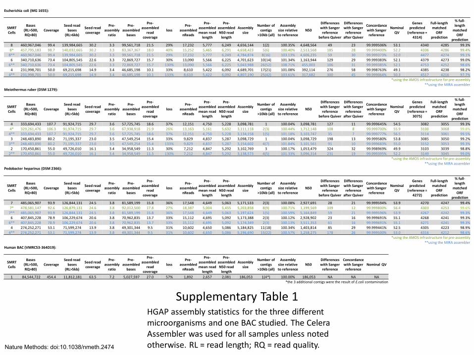
Supplementary Table 1 HGAP assembly statistics for the three different microorganisms and one BAC studied. The Celera Assembler was used for all samples unless noted otherwise. RL = read length; RQ = read quality.
Escherichia coli (MG 1655):
SMRT Cells
Bases (RL>500, RQ>80)
Coverage Seed read
bases (RL>6kb)
Seed read coverage
Pre-assembly
ratio
Pre-assembled
bases
Pre-assembled
read coverage
loss Pre-
assembled nReads
Pre-assembled mean read
length
Pre-assembled N50 read
length
Assembly size
Number of contigs
>10kb (all)
Assembly size relative to reference
N50
Differences with Sanger
reference before Quiver
Differences with Sanger reference
after Quiver
Concordance with Sanger reference
Nominal QV
Genes predicted
(reference = 4314)
Full-length matched
ORF prediction
% full-length
matched ORF
prediction
8 460,967,046 99.4 139,984,665 30.2 3.3 99,561,718 21.5 29% 17,232 5,777 6,249 4,656,144 1(2) 100.35% 4,648,564 49 23 99.999506% 53.1 4340 4285 99.3%
8* 457,795,183 98.7 140,032,665 30.2 3.3 83,367,367 18.0 40% 15,252 5,465 6,291 4,658,423 5(6) 100.40% 2,513,568 185 28 99.999400% 52.2 4336 4286 99.4%
8** 460,967,046 99.4 139,984,665 30.2 3.3 99,561,718 21.5 29% 17,232 5,777 6,249 4,784,874 8(16) 103.13% 4,606,235 59 30 99.999373% 52.0 4477 4274 99.1%
6 340,710,636 73.4 104,805,545 22.6 3.3 72,869,727 15.7 30% 13,090 5,566 6,225 4,701,623 10(14) 101.34% 1,163,944 129 29 99.999383% 52.1 4379 4273 99.0%
6** 340,710,636 73.4 104,805,545 22.6 3.3 72,869,727 15.7 130% 13,090 5,566 6,225 5,043,988 26(52) 108.71% 455,003 106 31 99.999385% 52.1 4753 4252 98.6%
4 231,998,701 50.0 69,215,698 14.9 3.4 46,685,198 10.1 33% 8,610 5,422 6,092 4,689,701 17(21) 101.08% 392,114 276 58 99.998763% 49.1 4385 4238 98.2%
4** 231,998,701 50.0 69,215,698 14.9 3.4 46,685,198 10.1 133% 8,610 5,422 6,092 4,807,190 25(42) 103.61% 317,682 300 45 99.999064% 50.3 4517 4216 97.7%
*using the AMOS infrastructure for pre-assembly
**using the MIRA assembler
Meiothermus ruber (DSM 1279):
SMRT Cells
Bases (RL>500, RQ>80)
Coverage Seed read
bases (RL>5kb)
Seed read coverage
Pre-assembly
ratio
Pre-assembled
bases
Pre-assembled
read coverage
loss Pre-
assembled nReads
Pre-assembled mean read
length
Pre-assembled N50 read
length
Assembly size
Number of contigs
>10kb (all)
Assembly size relative to reference
N50
Differences with Sanger
reference before Quiver
Differences with Sanger reference
after Quiver
Concordance with Sanger reference
Nominal QV
Genes predicted
(reference = 3075)
Full-length matched
ORF prediction
% full-length
matched ORF
prediction
4 333,694,433 107.7 91,924,715 29.7 3.6 57,725,745 18.6 37% 12,151 4,750 5,228 3,098,781 1 100.04% 3,098,781 127 11 99.999645% 54.5 3082 3055 99.3% 4* 329,261,476 106.3 91,974,715 29.7 3.6 67,938,918 21.9 26% 13,163 5,161 5,632 3,111,118 2(3) 100.44% 1,712,148 108 8 99.999700% 55.9 3100 3068 99.8%
4** 333,694,433 107.7 91,924,715 29.7 3.6 57,725,745 18.6 37% 12,151 4,750 5,228 3,134,158 1(5) 101.18% 3,103,747 35 7 99.999777% 56.5 3114 3061 99.5%
3 248,483,890 80.2 71,195,337 23.0 3.5 47,549,254 15.4 33% 9,829 4,837 5,287 3,098,729 1 100.04% 3,098,729 198 13 99.999580% 53.8 3085 3050 99.2%
3** 248,483,890 80.2 71,195,337 23.0 3.5 47,549,254 15.4 133% 9,829 4,837 5,287 3,154,602 4(7) 101.84% 3,101,561 91 10 99.999683% 55.0 3152 3053 99.3%
2 170,450,861 55.0 49,726,010 16.1 3.4 34,958,549 11.3 30% 7,212 4,847 5,292 3,102,769 3 100.17% 1,053,479 324 32 99.998969% 49.9 3103 3039 98.8%
2** 170,450,861 55.0 49,726,010 16.1 3.4 34,958,549 11.3 130% 7,212 4,847 5,292 3,138,573 4(5) 101.33% 3,096,314 231 19 99.999395% 52.2 3149 3045 99.0%
*using the AMOS infrastructure for pre-assembly
**using the MIRA assembler
Pedobacter heparinus (DSM 2366):
SMRT Cells
Bases (RL>500, RQ>80)
Coverage Seed read
bases (RL>5kb)
Seed read coverage
Pre-assembly
ratio
Pre-assembled
bases
Pre-assembled
read coverage
loss Pre-
assembled nReads
Pre-assembled mean read
length
Pre-assembled N50 read
length
Assembly size
Number of contigs
>10kb (all)
Assembly size relative to reference
N50
Differences with Sanger
reference before Quiver
Differences with Sanger reference
after Quiver
Concordance with Sanger reference
Nominal QV
Genes predicted
(reference = 4272)
Full-length matched
ORF prediction
% full-length
matched ORF
prediction
7 485,065,907 93.9 126,844,131 24.5 3.8 81,589,199 15.8 36% 17,548 4,649 5,063 5,171,533 2(3) 100.08% 2,927,691 28 21 99.999594% 53.9 4270 4247 99.4% 7* 478,581,147 92.6 126,879,131 24.6 3.8 92,012,500 17.8 27% 18,387 5,004 5,455 5,203,858 8(9) 100.71% 1,199,569 109 12 99.999800% 56.4 4303 4253 99.6%
7** 485,065,907 93.9 126,844,131 24.5 3.8 81,589,199 15.8 36% 17,548 4,649 5,063 5,197,624 1(5) 100.59% 5,164,849 59 21 99.999596% 53.9 4267 4242 99.3%
6 407,845,228 78.9 106,229,674 20.6 3.8 70,962,835 13.7 33% 15,112 4,695 5,092 5,173,388 2(3) 100.12% 2,928,902 23 16 99.999691% 55.1 4268 4241 99.3%
6** 407,845,228 78.9 106,229,674 20.6 3.8 70,962,835 13.7 33% 15,112 4,695 5,092 5,174,349 2(3) 100.13% 3,511,353 61 16 99.999691% 55.1 4271 4241 99.3%
4 274,252,271 53.1 71,599,274 13.9 3.8 49,301,344 9.5 31% 10,602 4,650 5,086 5,184,825 11(18) 100.34% 1,403,814 85 29 99.999441% 52.5 4305 4223 98.9%
4** 274,252,271 53.1 71,599,274 13.9 3.8 49,301,344 9.5 31% 10,602 4,650 5,086 5,196,690 15(22) 100.57% 1,258,275 178 26 99.999500% 53.0 4316 4212 98.6%
*using the AMOS infrastructure for pre-assembly
**using the MIRA assembler
Human BAC (VMRC53-364D19):
SMRT Cells
Bases (RL>500, RQ>80)
Coverage Seed read
bases (RL>5kb)
Seed read coverage
Pre-assembly
ratio
Pre-assembled
bases
Pre-assembled
read coverage
loss Pre-
assembled nReads
Pre-assembled mean read
length
Pre-assembled N50 read
length
Assembly size
Number of contigs
>10kb (all)
Assembly size relative to reference
N50 Differences with Sanger
reference
Concordance with Sanger reference
Nominal QV
1 84,544,722 454.4 11,812,181 63.5 7.2 5,027,597 27.0 57% 1,892 2,657 2,081 186,053 1(4*) 100.00% 186,053 NA NA NA
*the 3 additional contigs were the result of E.coli contamination
Nature Methods: doi:10.1038/nmeth.2474
Supplementary Table 2
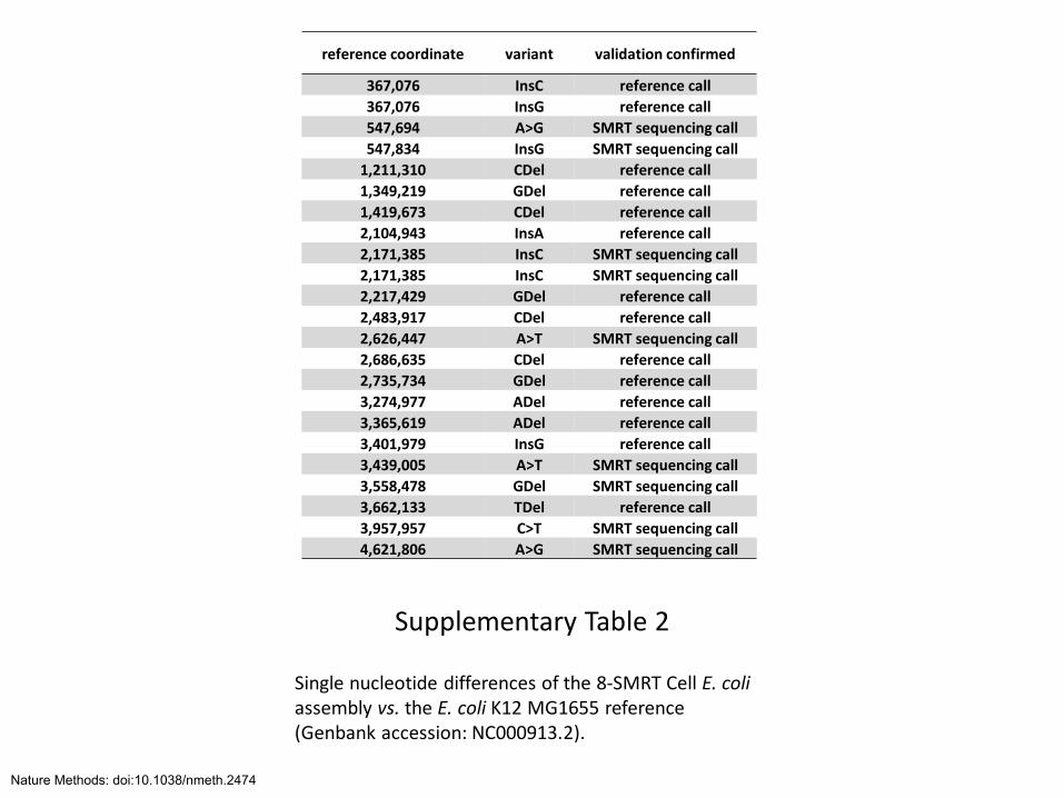
Single nucleotide differences of the 8-SMRT Cell E. coli assembly vs. the E. coli K12 MG1655 reference (Genbank accession: NC000913.2).
reference coordinate variant validation confirmed
367,076 InsC reference call
367,076 InsG reference call
547,694 A>G SMRT sequencing call
547,834 InsG SMRT sequencing call
1,211,310 CDel reference call
1,349,219 GDel reference call
1,419,673 CDel reference call
2,104,943 InsA reference call
2,171,385 InsC SMRT sequencing call
2,171,385 InsC SMRT sequencing call
2,217,429 GDel reference call
2,483,917 CDel reference call
2,626,447 A>T SMRT sequencing call
2,686,635 CDel reference call
2,735,734 GDel reference call
3,274,977 ADel reference call
3,365,619 ADel reference call
3,401,979 InsG reference call
3,439,005 A>T SMRT sequencing call
3,558,478 GDel SMRT sequencing call
3,662,133 TDel reference call
3,957,957 C>T SMRT sequencing call
4,621,806 A>G SMRT sequencing call
Nature Methods: doi:10.1038/nmeth.2474
Supplementary Table 3
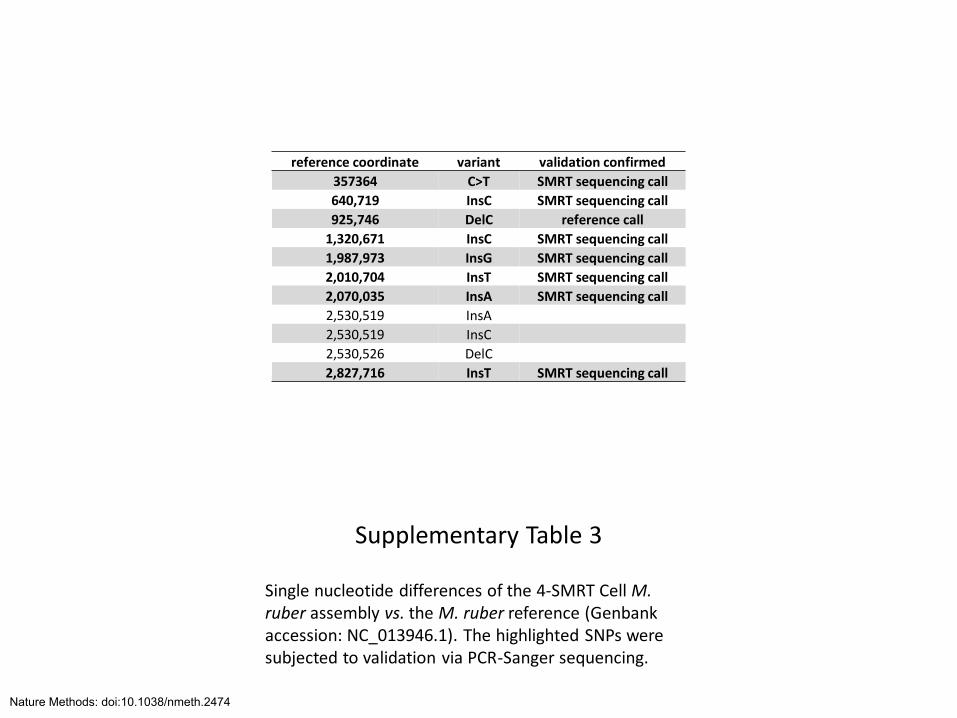
Single nucleotide differences of the 4-SMRT Cell M. ruber assembly vs. the M. ruber reference (Genbank accession: NC_013946.1). The highlighted SNPs were subjected to validation via PCR-Sanger sequencing.
reference coordinate variant validation confirmed
357364 C>T SMRT sequencing call
640,719 InsC SMRT sequencing call
925,746 DelC reference call
1,320,671 InsC SMRT sequencing call
1,987,973 InsG SMRT sequencing call
2,010,704 InsT SMRT sequencing call
2,070,035 InsA SMRT sequencing call
2,530,519 InsA
2,530,519 InsC
2,530,526 DelC
2,827,716 InsT SMRT sequencing call
Nature Methods: doi:10.1038/nmeth.2474
Supplementary Table 4
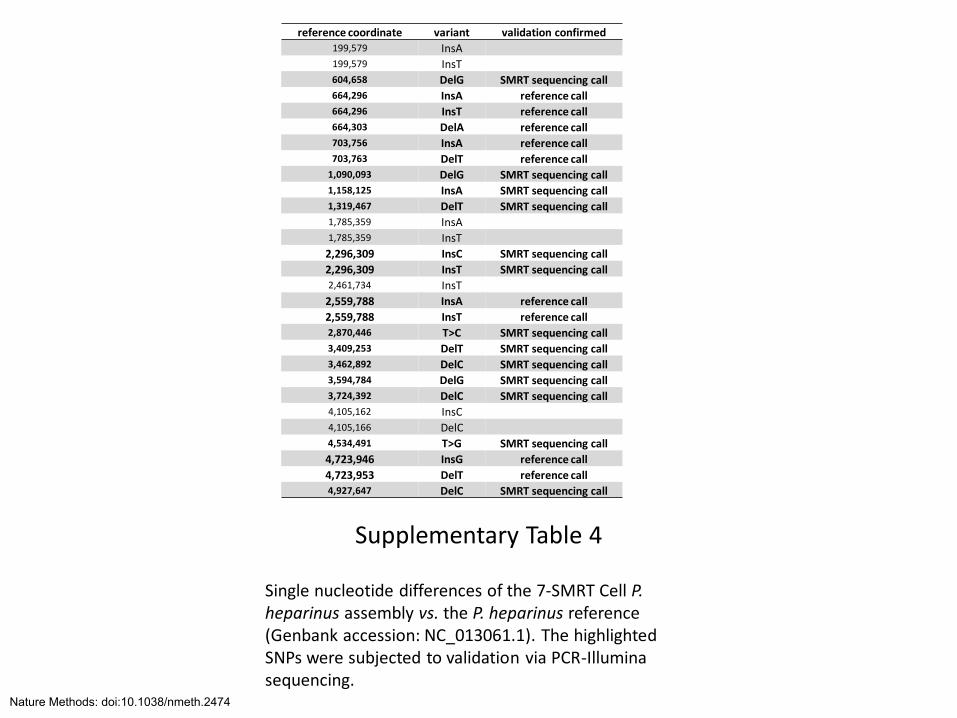
Single nucleotide differences of the 7-SMRT Cell P. heparinus assembly vs. the P. heparinus reference (Genbank accession: NC_013061.1). The highlighted SNPs were subjected to validation via PCR-Illumina sequencing.
reference coordinate variant validation confirmed 199,579 InsA 199,579 InsT 604,658 DelG SMRT sequencing call 664,296 InsA reference call 664,296 InsT reference call 664,303 DelA reference call 703,756 InsA reference call 703,763 DelT reference call
1,090,093 DelG SMRT sequencing call 1,158,125 InsA SMRT sequencing call 1,319,467 DelT SMRT sequencing call 1,785,359 InsA 1,785,359 InsT
2,296,309 InsC SMRT sequencing call
2,296,309 InsT SMRT sequencing call 2,461,734 InsT
2,559,788 InsA reference call
2,559,788 InsT reference call 2,870,446 T>C SMRT sequencing call 3,409,253 DelT SMRT sequencing call 3,462,892 DelC SMRT sequencing call 3,594,784 DelG SMRT sequencing call 3,724,392 DelC SMRT sequencing call 4,105,162 InsC 4,105,166 DelC 4,534,491 T>G SMRT sequencing call
4,723,946 InsG reference call
4,723,953 DelT reference call 4,927,647 DelC SMRT sequencing call
Nature Methods: doi:10.1038/nmeth.2474

Supplementary Table 5
Single-nucleotide variants in the VMRC53-364D19 BAC assembly vs. the hg19 reference that were validated using PCR-Sanger sequencing.
reference coordinate, chromosome 15
variant
32,394,062 TDel
32,364,043 TDel
32,310,527 T>C
32,387,828 T>C
32,340,851 G>T
32,338,206 A>C
Nature Methods: doi:10.1038/nmeth.2474
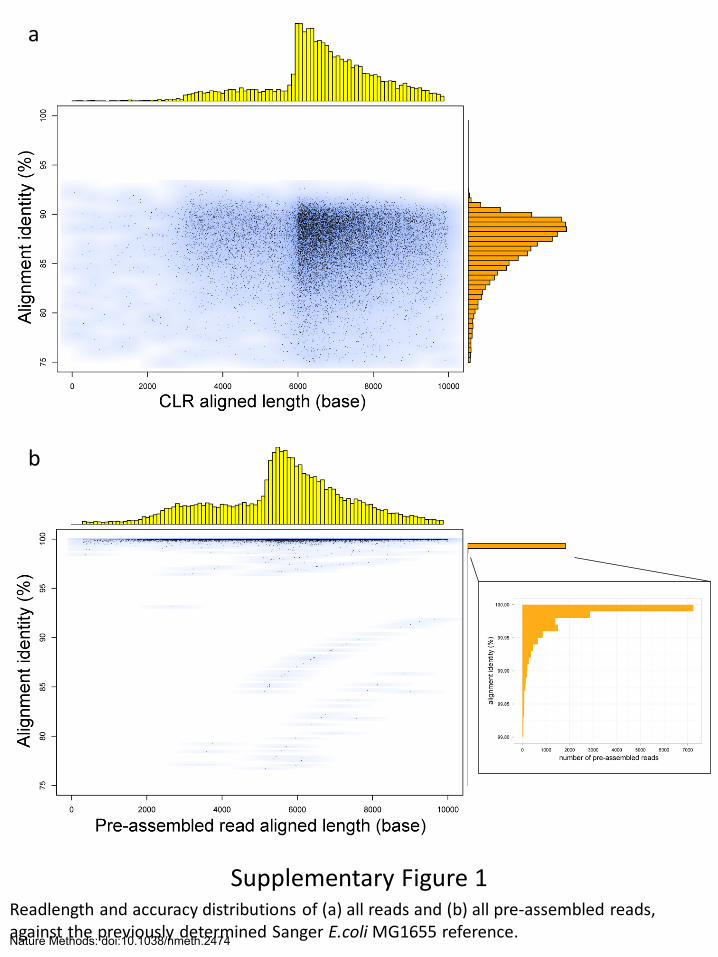
Supplementary Figure 1 Readlength and accuracy distributions of (a) all reads and (b) all pre-assembled reads, against the previously determined Sanger E.coli MG1655 reference.
a
b
Nature Methods: doi:10.1038/nmeth.2474
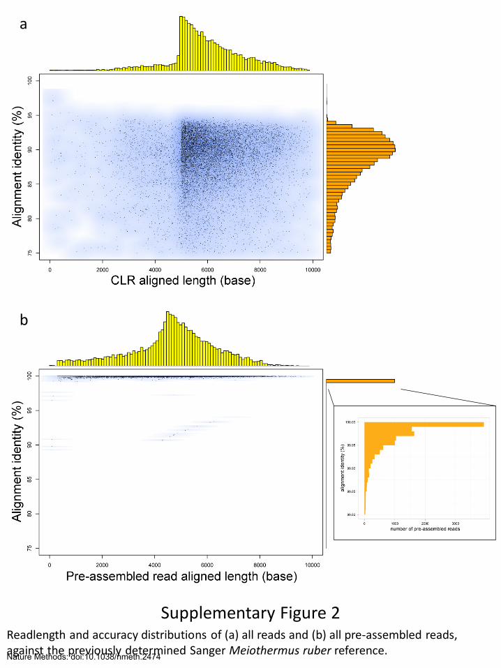
Supplementary Figure 2 Readlength and accuracy distributions of (a) all reads and (b) all pre-assembled reads, against the previously determined Sanger Meiothermus ruber reference.
a
b
Nature Methods: doi:10.1038/nmeth.2474
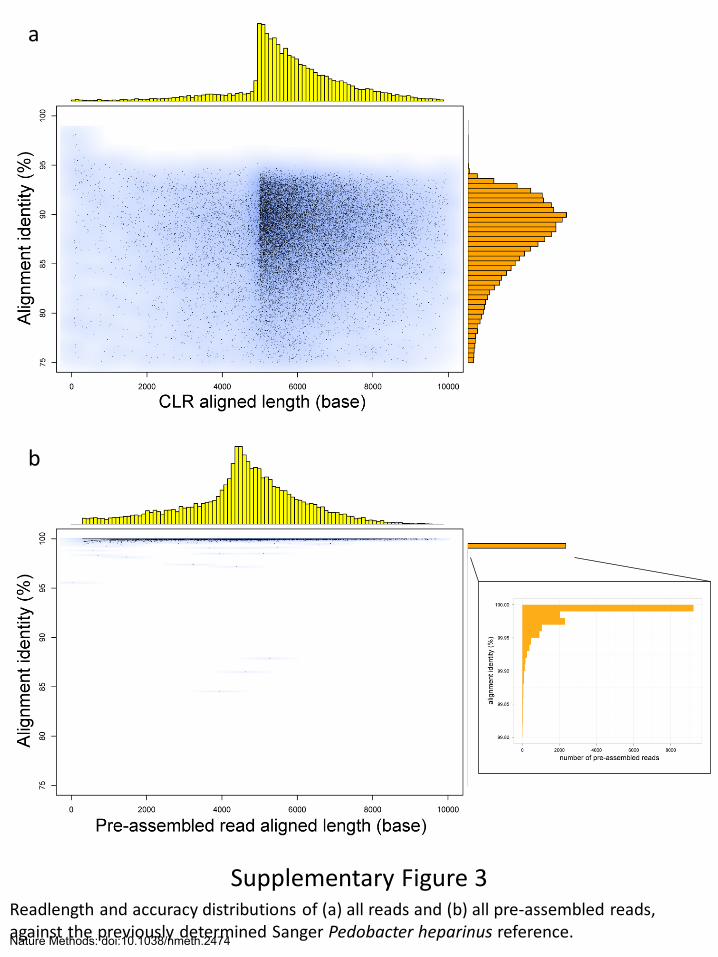
Supplementary Figure 3 Readlength and accuracy distributions of (a) all reads and (b) all pre-assembled reads, against the previously determined Sanger Pedobacter heparinus reference.
a
b
Nature Methods: doi:10.1038/nmeth.2474
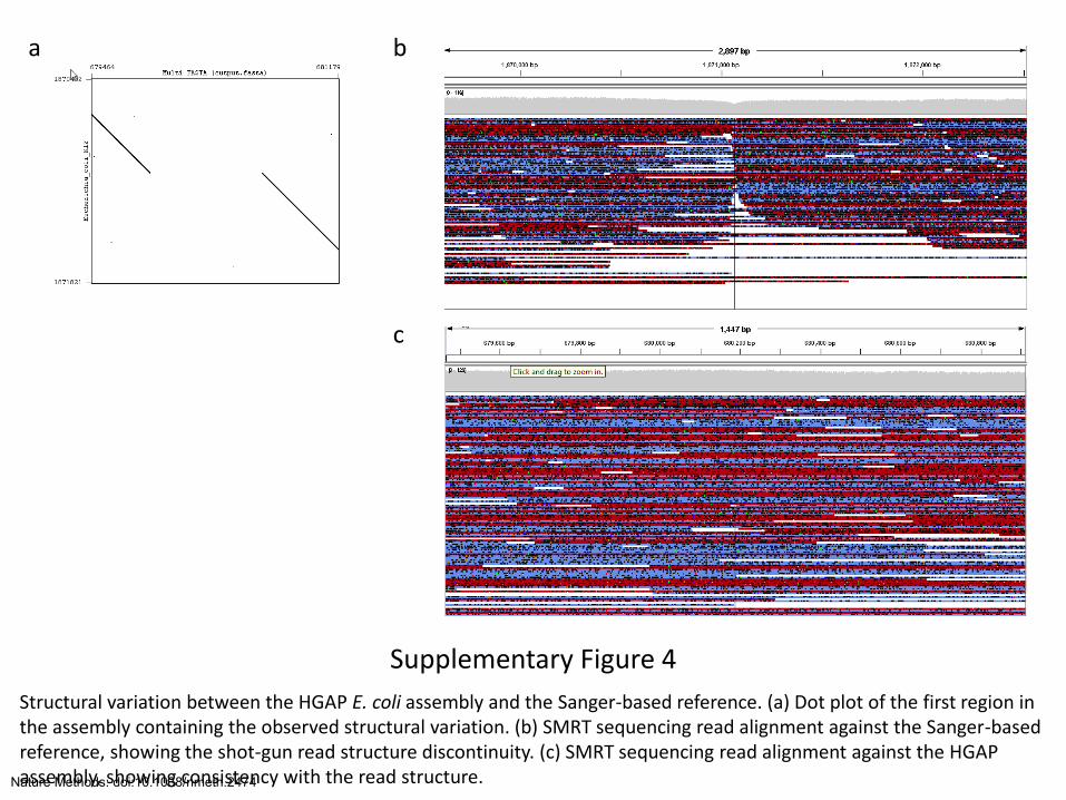
Supplementary Figure 4
Structural variation between the HGAP E. coli assembly and the Sanger-based reference. (a) Dot plot of the first region in the assembly containing the observed structural variation. (b) SMRT sequencing read alignment against the Sanger-based reference, showing the shot-gun read structure discontinuity. (c) SMRT sequencing read alignment against the HGAP assembly, showing consistency with the read structure.
a b
c
Nature Methods: doi:10.1038/nmeth.2474
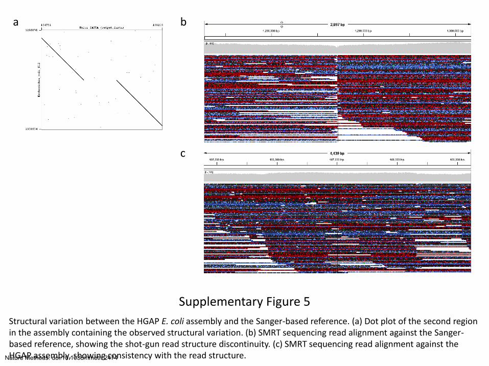
Supplementary Figure 5
Structural variation between the HGAP E. coli assembly and the Sanger-based reference. (a) Dot plot of the second region in the assembly containing the observed structural variation. (b) SMRT sequencing read alignment against the Sanger-based reference, showing the shot-gun read structure discontinuity. (c) SMRT sequencing read alignment against the HGAP assembly, showing consistency with the read structure.
a b
c
Nature Methods: doi:10.1038/nmeth.2474
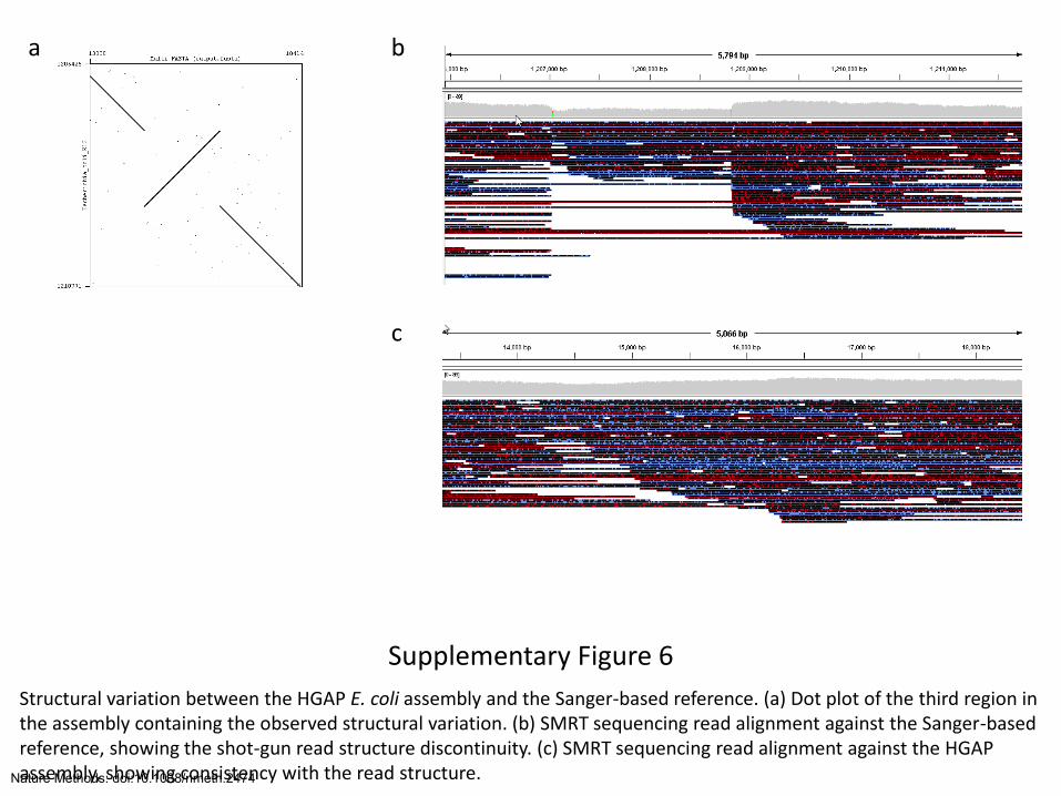
Supplementary Figure 6
Structural variation between the HGAP E. coli assembly and the Sanger-based reference. (a) Dot plot of the third region in the assembly containing the observed structural variation. (b) SMRT sequencing read alignment against the Sanger-based reference, showing the shot-gun read structure discontinuity. (c) SMRT sequencing read alignment against the HGAP assembly, showing consistency with the read structure.
a b
c
Nature Methods: doi:10.1038/nmeth.2474
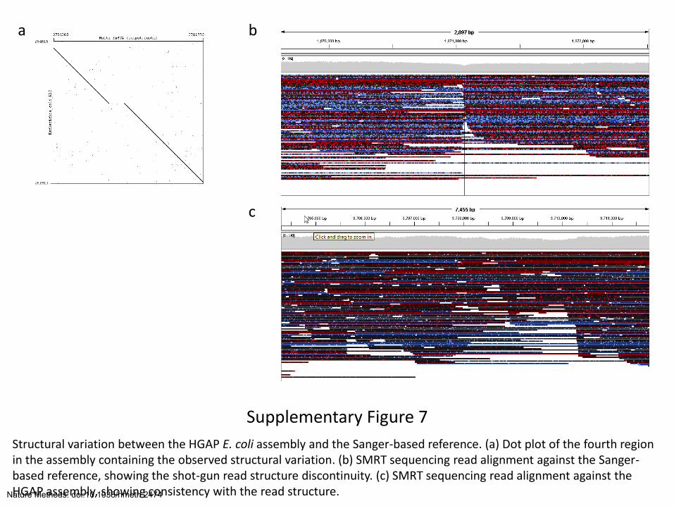
Supplementary Figure 7
Structural variation between the HGAP E. coli assembly and the Sanger-based reference. (a) Dot plot of the fourth region in the assembly containing the observed structural variation. (b) SMRT sequencing read alignment against the Sanger-based reference, showing the shot-gun read structure discontinuity. (c) SMRT sequencing read alignment against the HGAP assembly, showing consistency with the read structure.
a b
c
Nature Methods: doi:10.1038/nmeth.2474
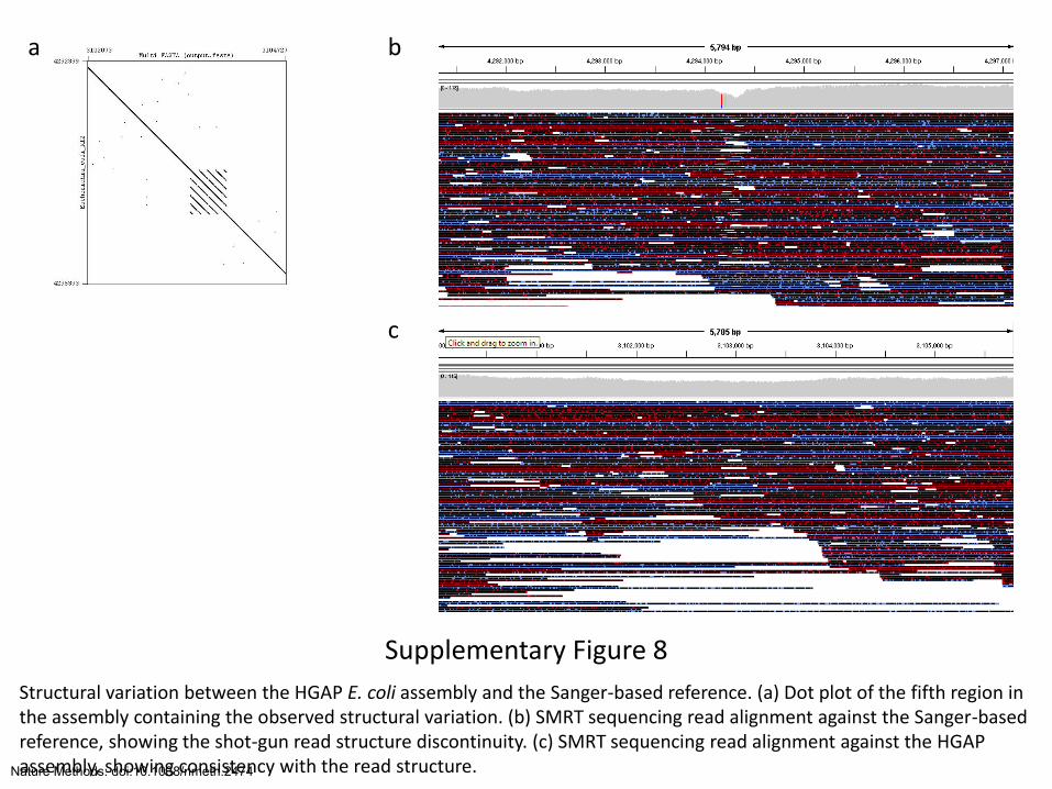
Supplementary Figure 8
Structural variation between the HGAP E. coli assembly and the Sanger-based reference. (a) Dot plot of the fifth region in the assembly containing the observed structural variation. (b) SMRT sequencing read alignment against the Sanger-based reference, showing the shot-gun read structure discontinuity. (c) SMRT sequencing read alignment against the HGAP assembly, showing consistency with the read structure.
a b
c
Nature Methods: doi:10.1038/nmeth.2474
8 SMRT Cell assembly
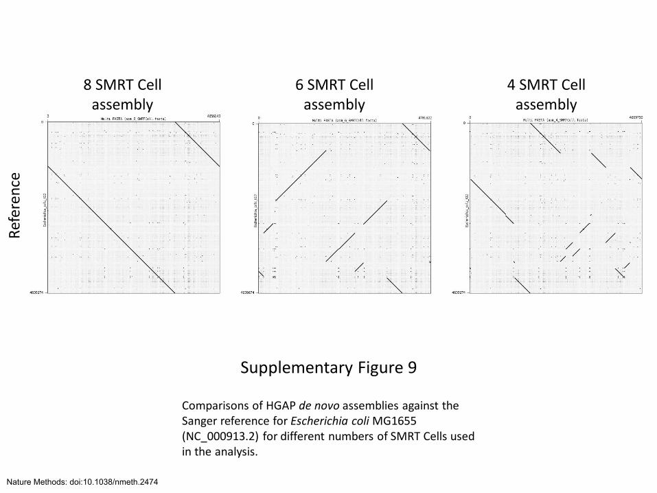
Supplementary Figure 9
Comparisons of HGAP de novo assemblies against the Sanger reference for Escherichia coli MG1655 (NC_000913.2) for different numbers of SMRT Cells used in the analysis.
Ref
eren
ce
6 SMRT Cell assembly
4 SMRT Cell assembly
Nature Methods: doi:10.1038/nmeth.2474
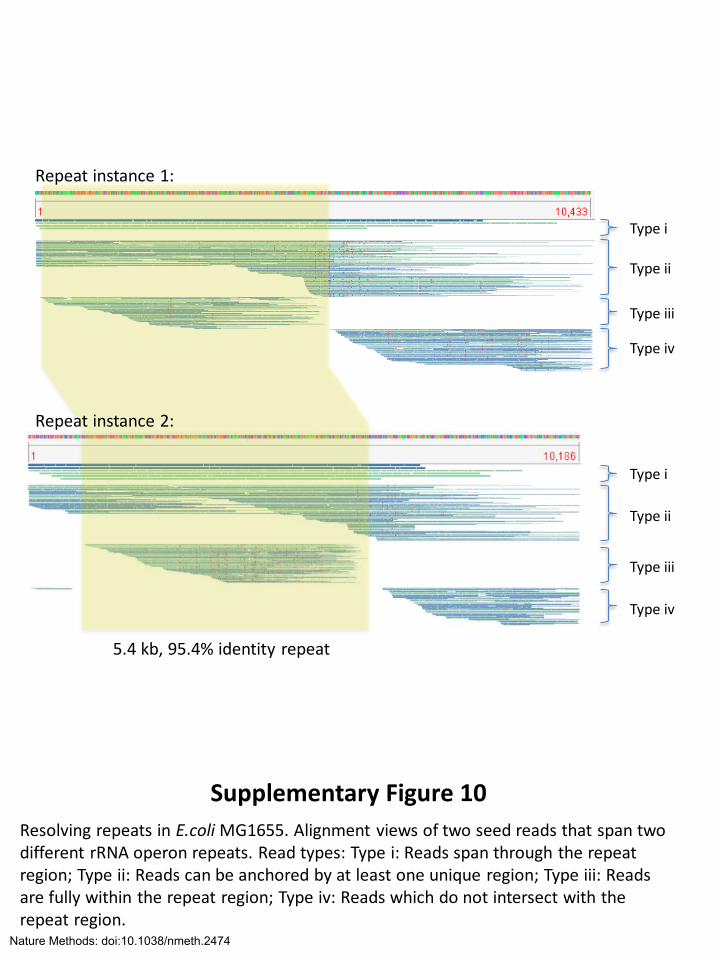
Supplementary Figure 10
Resolving repeats in E.coli MG1655. Alignment views of two seed reads that span two different rRNA operon repeats. Read types: Type i: Reads span through the repeat region; Type ii: Reads can be anchored by at least one unique region; Type iii: Reads are fully within the repeat region; Type iv: Reads which do not intersect with the repeat region.
5.4 kb, 95.4% identity repeat
Type i
Type ii
Type iii
Type iv
Type i
Type ii
Type iii
Type iv
Repeat instance 1:
Repeat instance 2:
Nature Methods: doi:10.1038/nmeth.2474

Supplementary Figure 11
Remapping of all CLRs for repeat 1 reads (blue) and repeat 2 reads (red) to the reference genome (a), and to the seed reads (b) in the E. coli MG1655 HGAP assembly.
a b
Nature Methods: doi:10.1038/nmeth.2474

Supplementary Figure 12
Comparisons of HGAP de novo assemblies against the Sanger reference for Meiothermus ruber (NC_013946.1) for different numbers of SMRT Cells used in the analysis.
Ref
eren
ce
4 SMRT Cell assembly
3 SMRT Cell assembly
2 SMRT Cell assembly
Nature Methods: doi:10.1038/nmeth.2474

Supplementary Figure 13
Comparisons of HGAP de novo assemblies against the Sanger reference for Pedobacter heparinus (NC_013061.1) for different numbers of SMRT Cells used in the analysis.
Ref
eren
ce
7 SMRT Cell assembly
6 SMRT Cell assembly
4 SMRT Cell assembly
Nature Methods: doi:10.1038/nmeth.2474
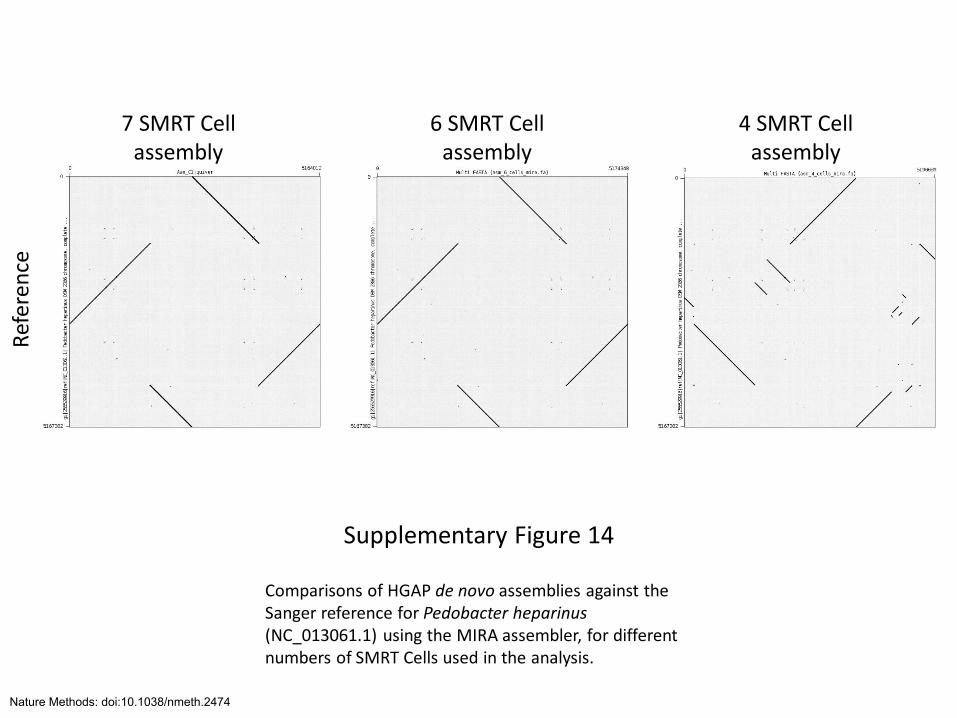
Supplementary Figure 14
Comparisons of HGAP de novo assemblies against the Sanger reference for Pedobacter heparinus (NC_013061.1) using the MIRA assembler, for different numbers of SMRT Cells used in the analysis.
Ref
eren
ce
7 SMRT Cell assembly
6 SMRT Cell assembly
4 SMRT Cell assembly
Nature Methods: doi:10.1038/nmeth.2474
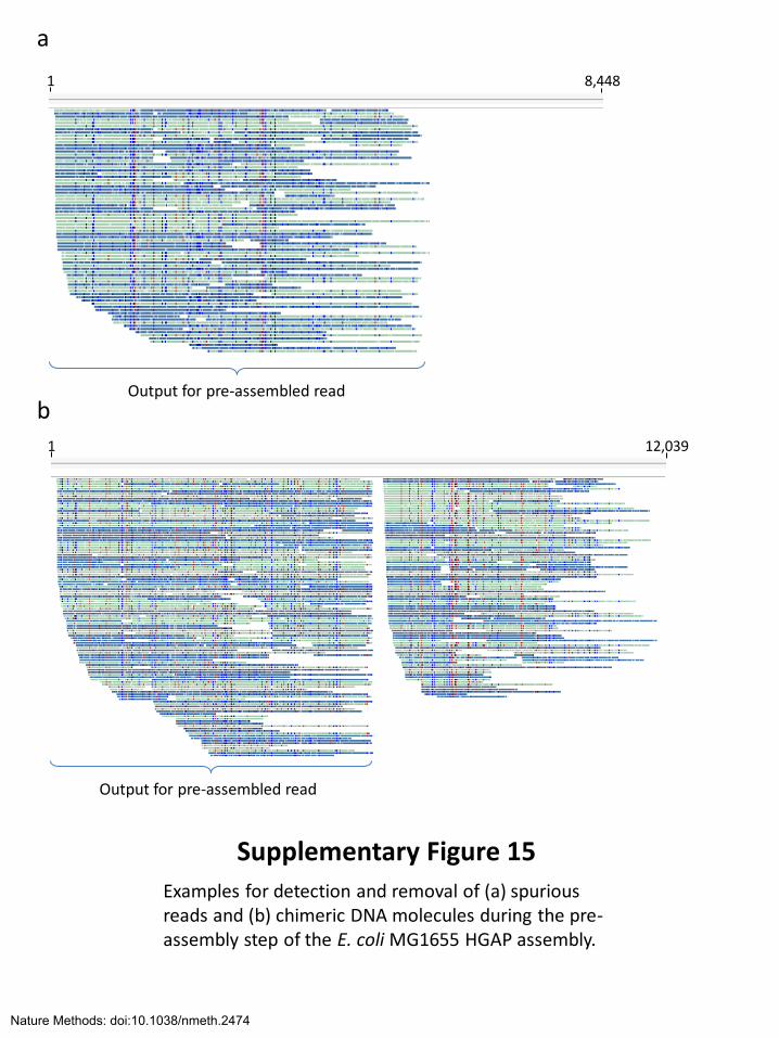
Supplementary Figure 15
Examples for detection and removal of (a) spurious reads and (b) chimeric DNA molecules during the pre-assembly step of the E. coli MG1655 HGAP assembly.
a
b
1 12,039
Output for pre-assembled read
1 8,448
Output for pre-assembled read
Nature Methods: doi:10.1038/nmeth.2474
Supplementary Note 1 to Chin et al. “Non-Hybrid, Finished
Microbial Genome Assemblies from Long-Read SMRT Sequencing
Data”
Contents
1 DAGCon: A Directed Acyclic Graph Based Consensus Algorithm 11.1 Outline of the SAG construction algorithm . . . . . . . . . . . . . . . . . . . . . . . 21.2 Normalize mismatches and degenerated alignment positions . . . . . . . . . . . . . . 31.3 Setup an initial graph from the reference sequence . . . . . . . . . . . . . . . . . . . 31.4 Construct the multigraph from the alignments and merge the edges . . . . . . . . . . 31.5 Merge nodes . . . . . . . . . . . . . . . . . . . . . . . . . . . . . . . . . . . . . . . . . 51.6 A Python implementation . . . . . . . . . . . . . . . . . . . . . . . . . . . . . . . . . 81.7 Generate consensus sequence from Gs . . . . . . . . . . . . . . . . . . . . . . . . . . 8
2 Using DAGCon Algorithm to Generate Pre-assembled Reads 10
3 Alternative Pre-assembly Method Using AMOS 11
4 Quiver Consensus Algorithm 134.1 Outline of the algorithm . . . . . . . . . . . . . . . . . . . . . . . . . . . . . . . . . . 134.2 Pulse metrics . . . . . . . . . . . . . . . . . . . . . . . . . . . . . . . . . . . . . . . . 144.3 Computing the template likelihood function, Pr(R | T ) . . . . . . . . . . . . . . . . . 144.4 Sketch of dynamic programming . . . . . . . . . . . . . . . . . . . . . . . . . . . . . 144.5 Alignment moves . . . . . . . . . . . . . . . . . . . . . . . . . . . . . . . . . . . . . . 154.6 Efficiently computing Pr(Rk | T + µ) . . . . . . . . . . . . . . . . . . . . . . . . . . 154.7 Banding optimization . . . . . . . . . . . . . . . . . . . . . . . . . . . . . . . . . . . 16
5 Evaluation of The Concordance of The Assemblies to The References 16
6 Gene Prediction Evaluation 16
1 DAGCon: A Directed Acyclic Graph Based Consensus Algo-rithm
We describe an algorithm of constructing directed acyclic graph from existing pairwise alignmentsused for the pre-assembly step in the current implementation for the hierarchical genome assemblyprocess. The algorithm presented here is motived by the original idea representing multiple sequence
1
Nature Methods: doi:10.1038/nmeth.2474
alignment as a directed acyclic graph proposed by Lee [Lee et al., 2002]. In Lee’s paper, the inputdata is just a collection of sequences and the partial order alignment (POA) is constructed byaligning the POA graph to a new added sequence in each iteration. In our applications, we usuallyknow about a candidate or a reference sequence and the goal is to identify differences betweensequencing reads and the reference sequence. The alignments between the sequence reads andthe reference are usually available from the earlier stages of the data processing pipeline by highperformance alignment software to map the reads to the reference. Such alignment data betweenthe reads and a reference is the input to the algorithm and is used to construct a directed acyclicgraph denoted as the sequence alignment graph (SAG). A SAG summarize all alignments from thereads to the reference sequence and is used to use to generate a consensus sequence that may bedifferent from the reference.
Under the assumptions that (1) the majority of variants are substitutions and (2) the sequencingerrors are usually mis-matches, a variant can be called by easily counting the read bases mappingthe a particular position in the reference sequence and a consensus sequence can be constructedby using the variant call and the reference sequence. When the characteristics sequencing datadoes not satisfy the assumptions (1) and (2), e.g. when insertions and deletions instead of mis-matches become the dominant error mode, it is necessary to go beyond counting the mismatches ofeach reference base. Instead, a multiple sequence alignment (MSA) is constructed and used to callvariants and build the consensus sequence. Complete optimized MSA construction is usually com-putationally expensive. Most MSA construction algorithms reported in the literature are mostlyfocusing on constructing a MSA within the context that there exist some evolution relations amongthe sequences [Edgar, 2004] [Larkin et al., 2007]. This may not be applicable to DNA sequencingapplication where the difference among the reads are due to random independent errors caused bythe sequencing reaction rather than some biological changes during the course of evolutional his-tory. It is therefore desirable to constructed a MSA to reflect such property of the sequencing readdata. For example, a consistency based multi-read alignment algorithm was developed for shortread assembly by Rausch et. al. [Rausch et al., 2009]. The construction of the SAG described hereuses only the alignments of the reads and the references such that all reads are treated equivalentlyin constructing the MSA. This is more suitable for generating consensus where all reads should betreated equally.
1.1 Outline of the SAG construction algorithm
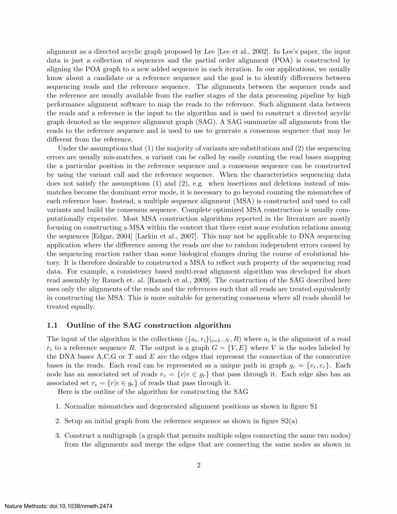
The input of the algorithm is the collections ({ai, ri}|i=1···N , R) where ai is the alignment of a readri to a reference sequence R. The output is a graph G = {V,E} where V is the nodes labeled bythe DNA bases A,C,G or T and E are the edges that represent the connection of the consecutivebases in the reads. Each read can be represented as a unique path in graph gr = {vr, er}. Eachnode has an associated set of reads rv = {r|v ∈ gr} that pass through it. Each edge also has anassociated set re = {r|e ∈ gr} of reads that pass through it.
Here is the outline of the algorithm for constructing the SAG
1. Normalize mismatches and degenerated alignment positions as shown in figure S1
2. Setup an initial graph from the reference sequence as shown in figure S2(a)
3. Construct a multigraph (a graph that permits multiple edges connecting the same two nodes)from the alignments and merge the edges that are connecting the same nodes as shown in
2
Nature Methods: doi:10.1038/nmeth.2474
figures S2(b) to S2(d)
4. According to the topological order of the node in the graph, systematically (1) merge nodesthat have the same label and are connected to the same node and (2) merge nodes that havethe same label and are connected from the same node as shown in figures S2(d) to S2(f)
read: CAC C-AC
| | → | |
ref: CGC CG-C
(a) Change mismatches into indels
read: CAACAT CAACAT
| | || → ||| |
ref: C-A-AT CAA--T
(b) Shift the equivalent gaps to the right in the reference
read: -C--CGT CCG--T
| | | → ||| |
ref: CCGAC-T CCGACT
(c) Shift the equivalent gaps to the right in the read
Figure S1: Examples of normalization of gaps in the alignment
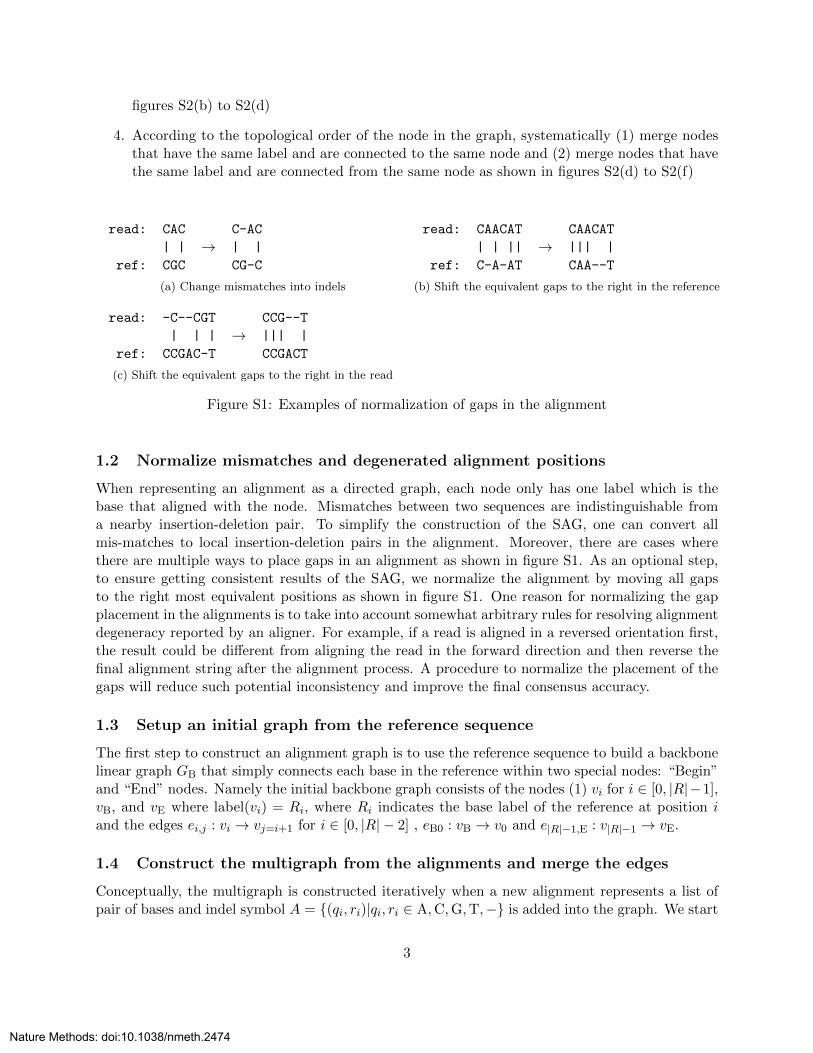
1.2 Normalize mismatches and degenerated alignment positions
When representing an alignment as a directed graph, each node only has one label which is thebase that aligned with the node. Mismatches between two sequences are indistinguishable froma nearby insertion-deletion pair. To simplify the construction of the SAG, one can convert allmis-matches to local insertion-deletion pairs in the alignment. Moreover, there are cases wherethere are multiple ways to place gaps in an alignment as shown in figure S1. As an optional step,to ensure getting consistent results of the SAG, we normalize the alignment by moving all gapsto the right most equivalent positions as shown in figure S1. One reason for normalizing the gapplacement in the alignments is to take into account somewhat arbitrary rules for resolving alignmentdegeneracy reported by an aligner. For example, if a read is aligned in a reversed orientation first,the result could be different from aligning the read in the forward direction and then reverse thefinal alignment string after the alignment process. A procedure to normalize the placement of thegaps will reduce such potential inconsistency and improve the final consensus accuracy.
1.3 Setup an initial graph from the reference sequence
The first step to construct an alignment graph is to use the reference sequence to build a backbonelinear graph GB that simply connects each base in the reference within two special nodes: “Begin”and “End” nodes. Namely the initial backbone graph consists of the nodes (1) vi for i ∈ [0, |R|−1],vB, and vE where label(vi) = Ri, where Ri indicates the base label of the reference at position iand the edges ei,j : vi → vj=i+1 for i ∈ [0, |R| − 2] , eB0 : vB → v0 and e|R|−1,E : v|R|−1 → vE.
1.4 Construct the multigraph from the alignments and merge the edges
Conceptually, the multigraph is constructed iteratively when a new alignment represents a list ofpair of bases and indel symbol A = {(qi, ri)|qi, ri ∈ A,C,G,T,−} is added into the graph. We start
3
Nature Methods: doi:10.1038/nmeth.2474
C
C C
C
G C
C
A A A
A
5 4 5 3 4 43
2
A A A
A
5 4 5 3 4 43
2
T T
C
C
G G C
read ATAT-AGCCGGCbackbone ATATTA---GGC
A A A
A
5 4 5 3 4 4
a
a
b
b
b
c
c read ATAT-AGCCGGCbackbone ATATTA---GGC
read ATAT-ACCGAG-backbone ATATTA--G-GC
read ATCAT--CCGGCbackbone AT-ATTA--GGC
read ATAT-ACGGCbackbone ATATTA-GGC
(a)
(b)
(c)
(d)
(e)
(f)
final consensus ATAT-ACCGGC backbone ATATTA--GGC
read ATAT-AGCCGGCbackbone ATATTA---GGC
A A AT T T G G C
A A AT T T
G
G G
C C
C
A A AT T T
G
G G
C C
C2 2 2 2 2
C
C
C C
C C
GG
G
T T T
TTT GG
G
C
C
C
C
T
2
2
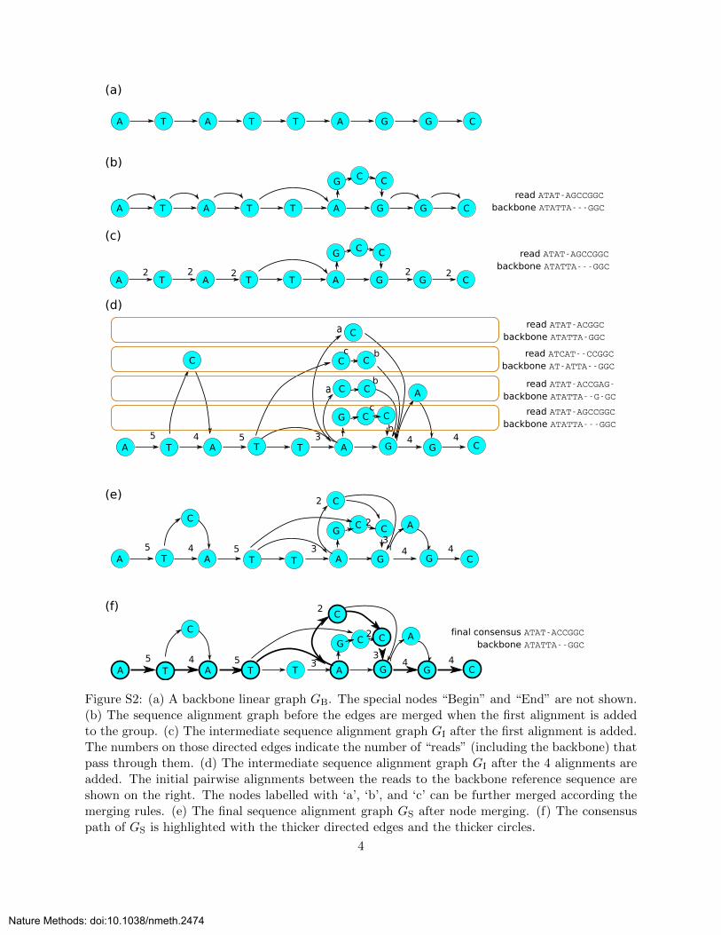
Figure S2: (a) A backbone linear graph GB. The special nodes “Begin” and “End” are not shown.(b) The sequence alignment graph before the edges are merged when the first alignment is addedto the group. (c) The intermediate sequence alignment graph GI after the first alignment is added.The numbers on those directed edges indicate the number of “reads” (including the backbone) thatpass through them. (d) The intermediate sequence alignment graph GI after the 4 alignments areadded. The initial pairwise alignments between the reads to the backbone reference sequence areshown on the right. The nodes labelled with ‘a’, ‘b’, and ‘c’ can be further merged according themerging rules. (e) The final sequence alignment graph GS after node merging. (f) The consensuspath of GS is highlighted with the thicker directed edges and the thicker circles.
4
Nature Methods: doi:10.1038/nmeth.2474
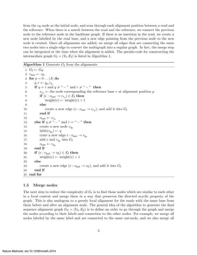
from the vB node as the initial node, and scan through each alignment position between a read andthe reference. When there is a match between the read and the reference, we connect the previousnode to the reference node in the backbone graph. If there is an insertion in the read, we create anew node labelled by the read base, and a new edge pointing from the previous node to the newnode is created. Once all alignments are added, we merge all edges that are connecting the sametwo nodes into a single edge to convert the multigraph into a regular graph. In fact, the merge stepcan be integrated at the time when the alignment is added. The pseudo-code for constructing theintermediate graph GI = (VI, EI) is listed in Algorithm 1.
Algorithm 1 Generate GI from the alignments
1: GI ← GB
2: vlast ← vB3: for p = 0 . . . |A| do4: q, r ← qp, rp5: if q = r and q 6= “− ” and r 6= “− ” then6: vrp ← the node corresponding the reference base r at alignment position p7: if (e : vlast → vrp) ∈ EI then8: weight(e)← weight(e) + 19: else
10: create a new edge (e : vlast → vrp), and add it into GI
11: end if12: vlast ← vrp13: else if q 6= “− ” and r = “− ” then14: create a new node vqp15: lable(vqp)← q16: crate a new edge e : vlast → vqp17: add e and vqp into GI
18: vlast ← vqp19: end if20: if (e : vlast → vE) ∈ EI then21: weight(e)← weight(e) + 122: else23: create a new edge (e : vlast → vE), and add it into GI
24: end if25: end for
1.5 Merge nodes
The next step to reduce the complexity of GI is to find those nodes which are similar to each otherin a local context and merge them in a way that preserves the directed acyclic property of thegraph. This is also analogous to a greedy local alignment for the reads with the same base fromthem before and after an alignment node. The general idea of the algorithm to generate the finalsequence alignment graph GS = (VS, ES) is to define an order to go through the graph and mergethe nodes according to their labels and connection to the other nodes. For example, we merge allnodes labeled by the same label and are connected to the same out-node, and we also merge all
5
Nature Methods: doi:10.1038/nmeth.2474

nodes with the same label that are connected from the same in-node. The algorithm presented hereis based on a variant of the topological sorting algorithm. The pseudocode is listed as Algorithm2,3,4. An example of showing the process is shown in figures S2(d) to (f).
Algorithm 2 Generate GS from GI
1: function in edges(v)2: return {e|u ∈ VS, (e : u→ v) ∈ ES}3: end function4: function out edges(v)5: return {e|u ∈ VS, (e : v → u) ∈ ES}6: end function7: function out nodes(v)8: return {u|u ∈ VS, (e : u→ v) ∈ in edges(v)}9: end function
10: function in nodes(v)11: return {u|u ∈ VS, (e : v → u) ∈ out edges(u)}12: end function13: GS ← GI
14: for all e ∈ GI do15: visited(e)← False16: end for17: s← an empty FIFO queue18: for v ∈ VS do19: if | in edges(v) | = 0 then20: push v into s21: end if22: end for23: while |s| 6= 0 do24: v ← pop(s)25: merge in node(v)26: merge out node(v)27: for all e ∈ out edges(v) do28: visited(e)← True29: end for30: for all u ∈ out nodes(v) do31: if |{e|e ∈ in edges(u), visited(e) = False}| = 0 then32: push u into s33: end if34: end for35: end while
6
Nature Methods: doi:10.1038/nmeth.2474
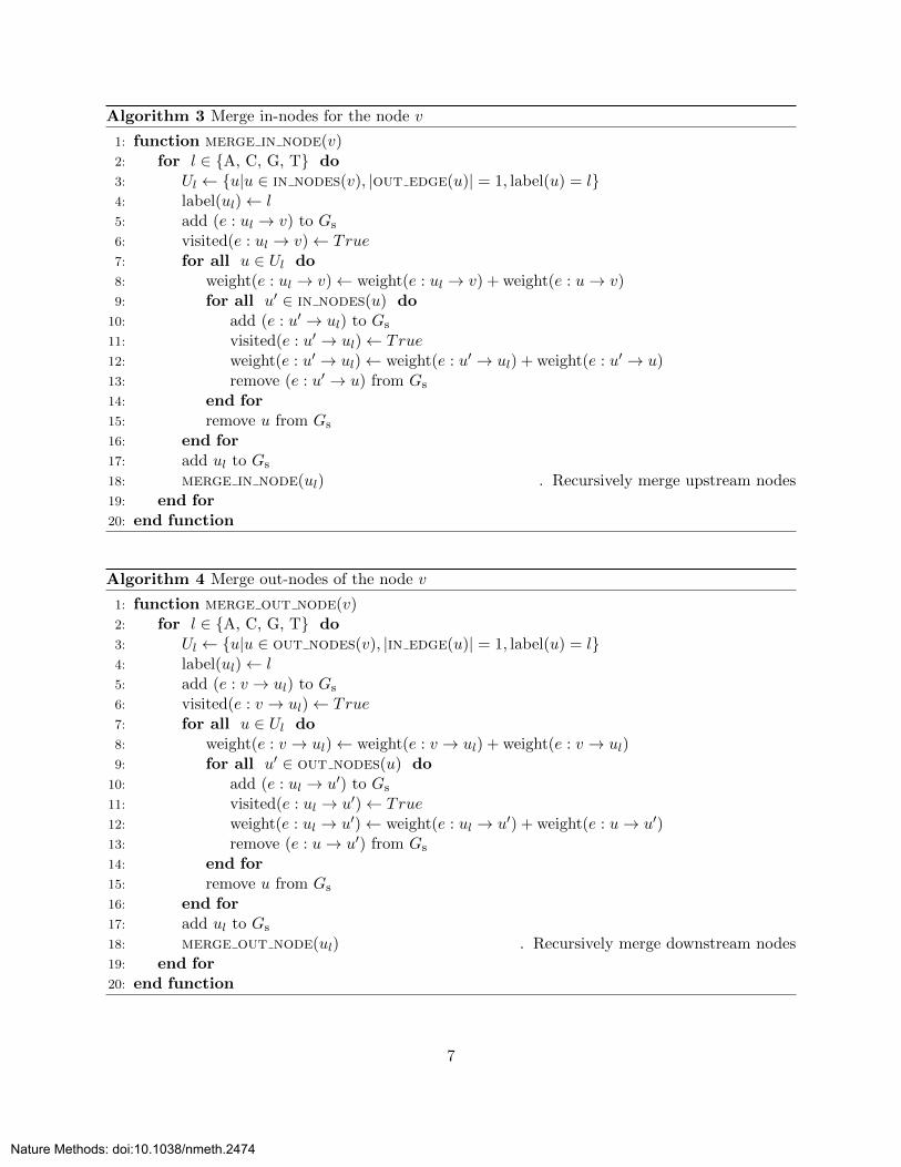
Algorithm 3 Merge in-nodes for the node v
1: function merge in node(v)2: for l ∈ {A, C, G, T} do3: Ul ← {u|u ∈ in nodes(v), |out edge(u)| = 1, label(u) = l}4: label(ul)← l5: add (e : ul → v) to Gs
6: visited(e : ul → v)← True7: for all u ∈ Ul do8: weight(e : ul → v)← weight(e : ul → v) + weight(e : u→ v)9: for all u′ ∈ in nodes(u) do
10: add (e : u′ → ul) to Gs
11: visited(e : u′ → ul)← True12: weight(e : u′ → ul)← weight(e : u′ → ul) + weight(e : u′ → u)13: remove (e : u′ → u) from Gs
14: end for15: remove u from Gs
16: end for17: add ul to Gs
18: merge in node(ul) . Recursively merge upstream nodes19: end for20: end function
Algorithm 4 Merge out-nodes of the node v
1: function merge out node(v)2: for l ∈ {A, C, G, T} do3: Ul ← {u|u ∈ out nodes(v), |in edge(u)| = 1, label(u) = l}4: label(ul)← l5: add (e : v → ul) to Gs
6: visited(e : v → ul)← True7: for all u ∈ Ul do8: weight(e : v → ul)← weight(e : v → ul) + weight(e : v → ul)9: for all u′ ∈ out nodes(u) do
10: add (e : ul → u′) to Gs
11: visited(e : ul → u′)← True12: weight(e : ul → u′)← weight(e : ul → u′) + weight(e : u→ u′)13: remove (e : u→ u′) from Gs
14: end for15: remove u from Gs
16: end for17: add ul to Gs
18: merge out node(ul) . Recursively merge downstream nodes19: end for20: end function
7
Nature Methods: doi:10.1038/nmeth.2474
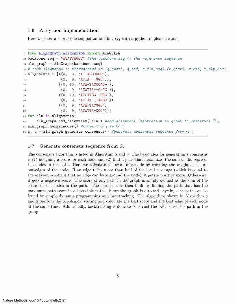
1.6 A Python implementation
Here we show a short code snippet on building GS with a python implementation.
1 from aligngraph.aligngraph import AlnGraph
2 backbone_seq = "ATATTAGGC" #the backbone_seq is the reference sequence
3 aln_graph = AlnGraph(backbone_seq)
4 # each alignment is represented as (q_start, q_end, q_aln_seq),(r_start, r_end, r_aln_seq),
5 alignments = [((0, 9, ’A-TAGCCGGC’),
6 (2, 9, ’ATTA---GGC’)),
7 ((0, 10, ’ATA-TACCGAG-’),
8 (0, 9, ’ATATTA--G-GC’)),
9 ((0, 10, ’ATCATCC--GGC’),
10 (0, 9, ’AT-AT--TAGGC’)),
11 ((0, 9, ’ATA-TACGGC’),
12 (0, 9, ’ATATTA-GGC’))]
13 for aln in alignments:
14 aln_graph.add_alignment( aln ) #add alignment information to graph to construct G I
15 aln_graph.merge_nodes() #convert G I to G S
16 s, c = aln_graph.generate_consensus() #generate consensus sequence from G S
1.7 Generate consensus sequence from Gs
The consensus algorithm is listed in Algorithm 5 and 6. The basic idea for generating a consensusis (1) assigning a score for each node and (2) find a path that maximizes the sum of the score ofthe nodes in the path. Here we calculate the score of a node by checking the weight of the allout-edges of the node. If an edge takes more than half of the local coverage (which is equal tothe maximum weight that an edge can have around the node), it gets a positive score. Otherwise,it gets a negative score. The score of any path in the graph is simply defined as the sum of thescores of the nodes in the path. The consensus is then built by finding the path that has themaximum path score in all possible paths. Since the graph is directed acyclic, such path can befound by simple dynamic programming and backtracking. The algorithms shown in Algorithm 5and 6 perform the topological sorting and calculate the best score and the best edge of each nodeat the same time. Additionally, backtracking is done to construct the best consensus path in thegroup.
8
Nature Methods: doi:10.1038/nmeth.2474

Algorithm 5 Find the best path in Gs as the consensus sequence
1: s← an empty FIFO queue2: for all v ∈ Vs do3: if |out edges(v)| = 0 then4: put v into s5: best out edge(v)← ∅6: best in edge(v)← ∅7: node score(v)← 08: end if9: end for
10: for all e ∈ Es do11: visited(e)← False12: end for13: while |s| 6= 0 do14: v ← pop(s)15: ebest ← ∅16: scorebest ← ∅17: for (eout : v → u) ∈ out edges(v) do . find the best out-edge for node v18: score← node score(u)19: coverage← the local coverage for the node u20: if u ∈ VB then21: scorenew ← score− δ . choose δ (default δ = 10) to make the path along the
reference unfavorable22: else23: scorenew ← weight(eout)− coverage ∗ 0.5 + score24: end if25: if scorebest is ∅ or scorenew > scorebest then26: ebest ← eout27: scorebest ← scorenew28: end if29: end for30: if ebest 6= ∅ then31: best score edge(v) = ebest32: node score(v)← scorebest33: end if34: for e ∈ in edges(v) do35: visited(e)← True36: end for37: for all u ∈ in nodes(v) do38: if |{e|e ∈ out edges(u), visited(e) = False}| = 0 then39: push u into s40: end if41: end for42: end while
9
Nature Methods: doi:10.1038/nmeth.2474

Algorithm 6 Find the best path in Gs as the consensus sequence (cont.)
43: v ← vB44: consensus path← empty list45: while True do46: append v to consensus path47: if v has no best score edge then48: Break49: else50: (ebest out : v → u)← best score edge(v)51: v ← u52: end if53: end while
Such consensus algorithm is typically “biased” toward to the reference used in the alignment.If the real sample sequences have high variation from the reference sequence, then there will beopportunity for further improvement from the single-pass consensus algorithm. One way to improveit is to use an iterative process to increase the final quality of the consensus sequence. Namely,one can take the consensus sequence as the reference sequence and align the reads back to thefirst iteration of the consensus sequence and repeatedly apply the consensus algorithm to generatethe next iteration of the consensus sequences. Such iteration process can reconstruct the regionsthat are very different from the original reference, although it is generally more computationallyintensive. The other possible strategy is to identify the high variation region, then, rather thanusing the original reference, one uses one of the reads as the reference to reconstruct those regionsto avoid the “bias” toward the original reference.
2 Using DAGCon Algorithm to Generate Pre-assembled Reads
We first mapped all subreads to the long seeding set using blasr. We split the target seedingsequences into chunks for mapping other reads to them in parallel. In such case, we use thefollow blasr options for mapping: “-nCandidates 50 -minMatch 12 -maxLCPLength 15 -bestn
5 -minPctIdentity 70.0 -maxScore -1000 -m 4”. After mapping, the blasr output files areparsed for each chunk and top 12 hits are selected for each query reads as default. The number oftop hits could impact the quality of the pre-assembly reads and the ability to resolve very similarrepeats.
For each seed read, we collect the all subreads aligned to it from the alignment output of theblasr program. Each subread are trimmed according to the alignment coordinates. For example,if blasr reports base s1 to s2 are aligned to the seed read, we will use base s1 + ∆ to s2 − ∆ forpre-assembly. We choose ∆ to be 100 since the blasr aligner sometimes generate poor alignmentat the ends such that chimera reads might still have good coverage across the chimeric junction.More aggressive trimming with a larger ∆ will help to remove all chimeric reads at a cost losinguseful bases. One can avoid losing base by choosing smaller ∆.
The trimmed subreads are then used with the seed read to generate the pre-assembled readwith the DAGCon algorithm described in the previous section.
A benchmark run was performed with Amazon EC2 cloud computing service. It took about 1.5hours on a virtual cluster of 8 c1.xlarge instances (8 virtual cores with 2.5 EC2 Compute Units
10
Nature Methods: doi:10.1038/nmeth.2474

each instance) for the mapping step between the reads using blasr and 7 hours for the DAGConstep in the same virtual cluster for the 8 SMRTCell E. coli dataset. The pure python basedDAGCon code can be accelerated by declaring the type of each variable to reduce the dynamicaltyping resolution overhead with Cython (http://www.cython.org). A test version of DAGConimplemented with Cython from the same code base used only 1 hour in the same cluster for thepre-assembly step. The detailed steps on how to set the running environment can be found athttp://pacb.com/devnet/files/software/hgap/HGAP README.rst andhttp://pacb.com/devnet/files/software/hgap/Starcluster instruction.rst.
3 Alternative Pre-assembly Method Using AMOS
To demonstrate the generality of the HGAp methodology, we demonstrate that we can also useBLASR and tools from the AMOS assembly toolkit as part of the 1.4 Pacific Biosciences SMRTAnalysis software package to test it on the Pedobacter heparinus genome.
In this process, all continuous long reads from E. coli (8 SMRT cells), M. ruber (4 SMRT cells),and P. heparinus (7 SMRT cells) genomes were aligned to those reads of length greater than 5kbusing BLASR with the following options:
-minReadLength 200 -maxScore -1000 -bestn 24 -maxLCPLength 16 -nCandidates 24
These alignments were used to arrange reads in AMOS layout messages, which were uploadedto an AMOS bank along with the read sequences and quality values. Importantly, the layoutscontained only the portion of each read that aligned to that particular CLR seed read, trimmed by50bp on each side of the alignment. Reads were kept in the same layout if these trimmed alignedportions overlapped by at least 100bp, otherwise they were split into multiple layouts. Consensussequence was generated using the off-the-shelf AMOS executable make-consensus with the followingoption: -L.
The resulting consensus sequences were trimmed to regions with greater than 59.5 average QV(as called by the make-consensus algorithm) and greater than 500bp in length. These pre-assembledreads were evaluated and further assembled into contigs using the Celera Assembler and correctedusing Quiver in a manner identical to the other pre-assembled read data sets in SupplementaryTable 1. The software used to perform the read pre-assembly will be available as a command linetool and a SMRT Portal protocol in the 1.4 release of Pacific Biosciences SMRT Analysis software.The SMRT Pipe parameter file necessary for regenerating these results is included here:
1 <smrtpipeSettings>
2 <module name="P_Fetch"/>
3 <module name="P_Filter">
4 <param name="minLength">
5 <value>50</value>
6 </param>
7 <param name="minSubReadLength">
8 <value>500</value>
9 </param>
10 <param name="readScore">
11
Nature Methods: doi:10.1038/nmeth.2474

11 <value>0.80</value>
12 </param>
13 </module>
14 <module name="P_FilterReports"/>
15 <module name="P_ErrorCorrection">
16 <param name="useFastqAsShortReads">
17 <value>False</value>
18 </param>
19 <param name="useFastaAsLongReads">
20 <value>False</value>
21 </param>
22 <param name="useLongReadsInConsensus">
23 <value>False</value>
24 </param>
25 <param name="useUnalignedReadsInConsensus">
26 <value>False</value>
27 </param>
28 <param name="useCCS">
29 <value>False</value>
30 </param>
31 <param name="minLongReadLength">
32 <value>5000</value>
33 </param>
34 <param name="blasrOpts">
35 <value> -minReadLength 200 -minPctIdentity 75 -maxScore -100 -bestn 24
36 -maxLCPLength 16 -nCandidates 24 </value>
37 </param>
38 <param name="consensusOpts">
39 <value> -L </value>
40 </param>
41 <param name="layoutOpts">
42 <value> --overlapTolerance 100 --trimHit 50 </value>
43 </param>
44 <param name="consensusChunks">
45 <value>60</value>
46 </param>
47 <param name="trimFastq">
48 <value>True</value>
49 </param>
50 <param name="trimOpts">
51 <value> --qvCut=59.5 --minSeqLen=500 </value>
52 </param>
53 </module>
54 </smrtpipeSettings>
12
Nature Methods: doi:10.1038/nmeth.2474
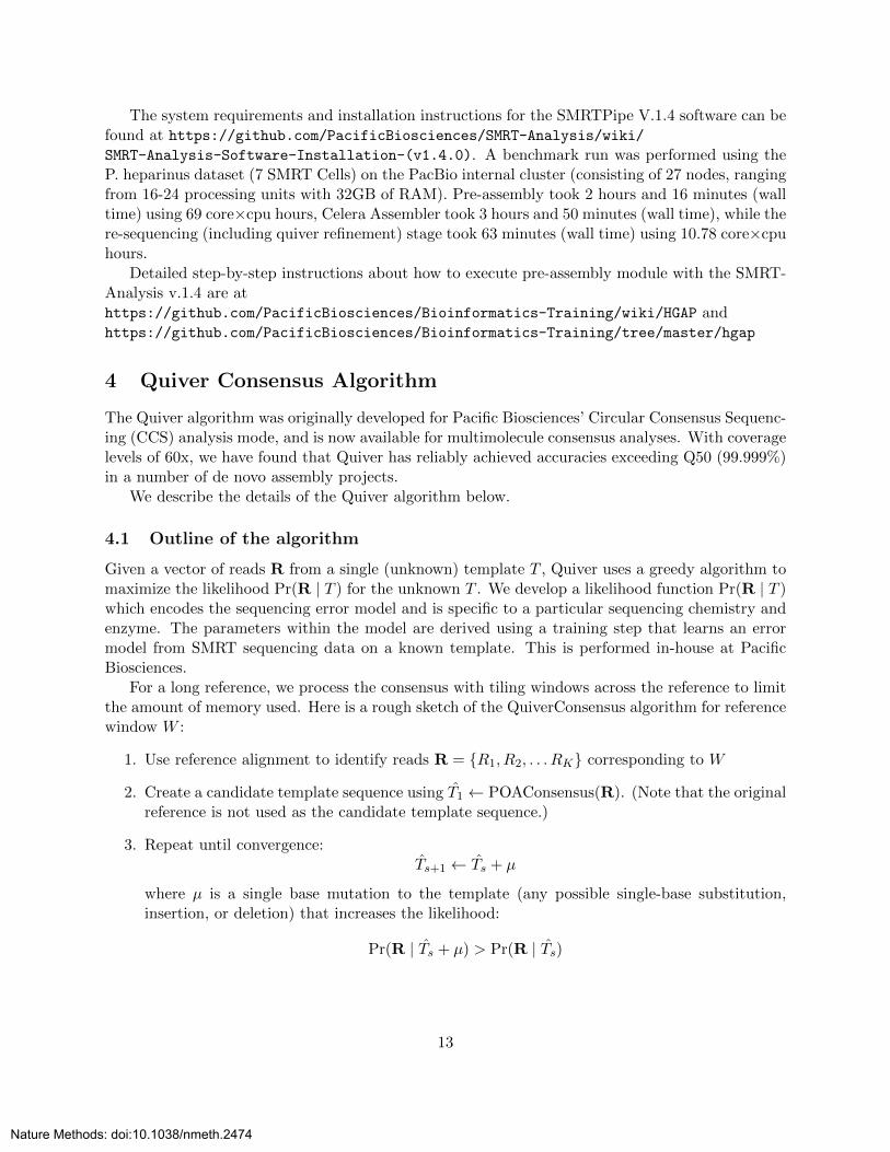
The system requirements and installation instructions for the SMRTPipe V.1.4 software can befound at https://github.com/PacificBiosciences/SMRT-Analysis/wiki/SMRT-Analysis-Software-Installation-(v1.4.0). A benchmark run was performed using theP. heparinus dataset (7 SMRT Cells) on the PacBio internal cluster (consisting of 27 nodes, rangingfrom 16-24 processing units with 32GB of RAM). Pre-assembly took 2 hours and 16 minutes (walltime) using 69 core×cpu hours, Celera Assembler took 3 hours and 50 minutes (wall time), while there-sequencing (including quiver refinement) stage took 63 minutes (wall time) using 10.78 core×cpuhours.
Detailed step-by-step instructions about how to execute pre-assembly module with the SMRT-Analysis v.1.4 are athttps://github.com/PacificBiosciences/Bioinformatics-Training/wiki/HGAP andhttps://github.com/PacificBiosciences/Bioinformatics-Training/tree/master/hgap
4 Quiver Consensus Algorithm
The Quiver algorithm was originally developed for Pacific Biosciences’ Circular Consensus Sequenc-ing (CCS) analysis mode, and is now available for multimolecule consensus analyses. With coveragelevels of 60x, we have found that Quiver has reliably achieved accuracies exceeding Q50 (99.999%)in a number of de novo assembly projects.
We describe the details of the Quiver algorithm below.
4.1 Outline of the algorithm
Given a vector of reads R from a single (unknown) template T , Quiver uses a greedy algorithm tomaximize the likelihood Pr(R | T ) for the unknown T . We develop a likelihood function Pr(R | T )which encodes the sequencing error model and is specific to a particular sequencing chemistry andenzyme. The parameters within the model are derived using a training step that learns an errormodel from SMRT sequencing data on a known template. This is performed in-house at PacificBiosciences.
For a long reference, we process the consensus with tiling windows across the reference to limitthe amount of memory used. Here is a rough sketch of the QuiverConsensus algorithm for referencewindow W :
1. Use reference alignment to identify reads R = {R1, R2, . . . RK} corresponding to W
2. Create a candidate template sequence using T̂1 ← POAConsensus(R). (Note that the originalreference is not used as the candidate template sequence.)
3. Repeat until convergence:T̂s+1 ← T̂s + µ
where µ is a single base mutation to the template (any possible single-base substitution,insertion, or deletion) that increases the likelihood:
Pr(R | T̂s + µ) > Pr(R | T̂s)
13
Nature Methods: doi:10.1038/nmeth.2474
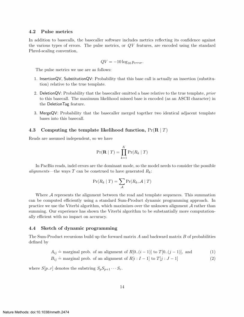
4.2 Pulse metrics
In addition to basecalls, the basecaller software includes metrics reflecting its confidence againstthe various types of errors. The pulse metrics, or QV features, are encoded using the standardPhred-scaling convention,
QV = −10 log10 perror.
The pulse metrics we use are as follows:
1. InsertionQV, SubstitutionQV: Probability that this base call is actually an insertion (substitu-tion) relative to the true template.
2. DeletionQV: Probability that the basecaller omitted a base relative to the true template, priorto this basecall. The maximum likelihood missed base is encoded (as an ASCII character) inthe DeletionTag feature.
3. MergeQV: Probability that the basecaller merged together two identical adjacent templatebases into this basecall.
4.3 Computing the template likelihood function, Pr(R | T )
Reads are assumed independent, so we have
Pr(R | T ) =K∏k=1
Pr(Rk | T )
In PacBio reads, indel errors are the dominant mode, so the model needs to consider the possiblealignments—the ways T can be construed to have generated Rk:
Pr(Rk | T ) =∑A
Pr(Rk,A | T )
Where A represents the alignment between the read and template sequences. This summationcan be computed efficiently using a standard Sum-Product dynamic programming approach. Inpractice we use the Viterbi algorithm, which maximizes over the unknown alignment A rather thansumming. Our experience has shown the Viterbi algorithm to be substantially more computation-ally efficient with no impact on accuracy.
4.4 Sketch of dynamic programming
The Sum-Product recursions build up the forward matrix A and backward matrix B of probabilitiesdefined by
Aij.= marginal prob. of an alignment of R[0..(i− 1)] to T [0..(j − 1)], and (1)
Bij.= marginal prob. of an alignment of R[i : I − 1] to T [j : J − 1] (2)
where S[p..r] denotes the substring SpSp+1 · · ·Sr.
14
Nature Methods: doi:10.1038/nmeth.2474
The recursions are computed as
Aij =∑
m:(i′,j′)→(i,j)
(Ai′j′ ×moveScore(m)), and (3)
Bij =∑
m:(i,j)→(i′,j′)
(moveScore(m)×Bi′j′) (4)
For the Viterbi algorithm, replace marginal by maximum and sum by max in the above defini-tions.
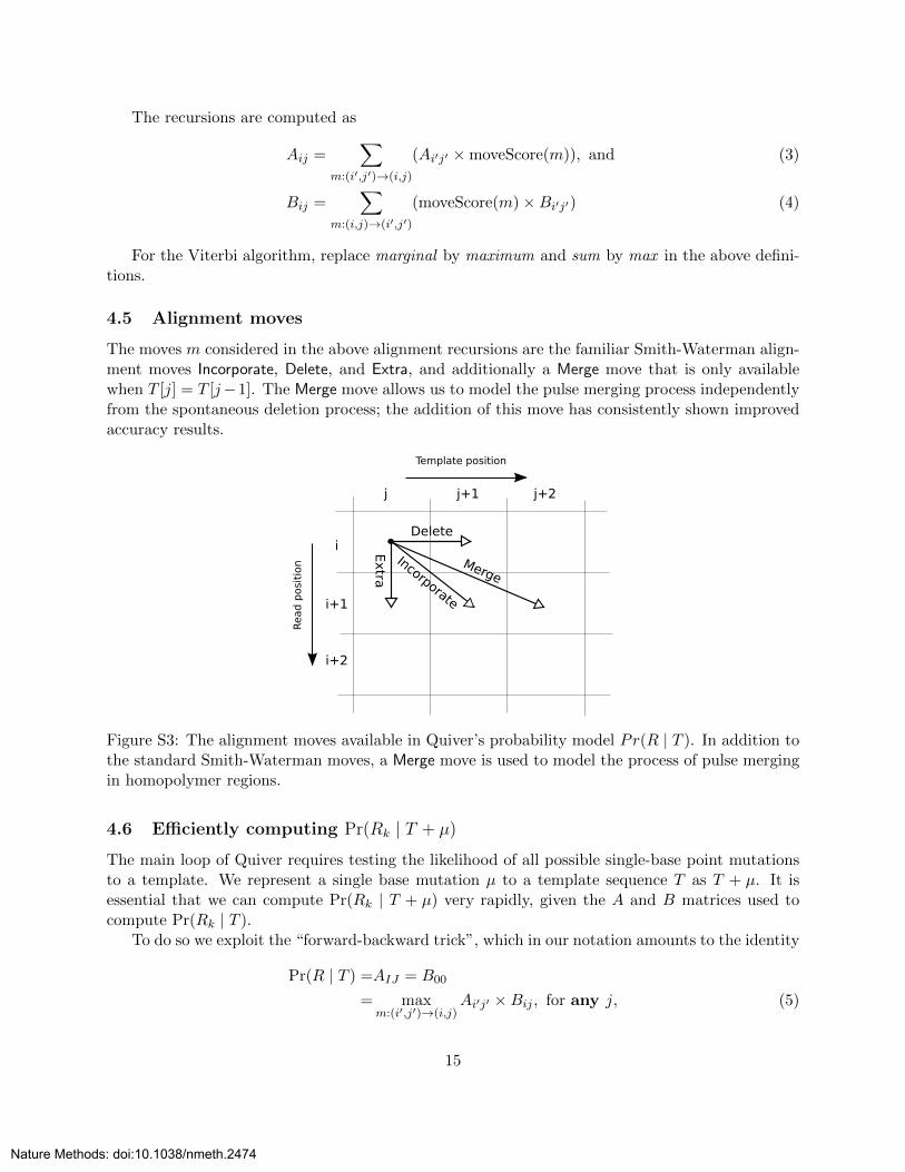
4.5 Alignment moves
The moves m considered in the above alignment recursions are the familiar Smith-Waterman align-ment moves Incorporate, Delete, and Extra, and additionally a Merge move that is only availablewhen T [j] = T [j−1]. The Merge move allows us to model the pulse merging process independentlyfrom the spontaneous deletion process; the addition of this move has consistently shown improvedaccuracy results.
Template position
Read
posi
tion
j j+1 j+2
i
i+1
i+2
DeleteExtra
Incorporate
Merge
Figure S3: The alignment moves available in Quiver’s probability model Pr(R | T ). In addition tothe standard Smith-Waterman moves, a Merge move is used to model the process of pulse mergingin homopolymer regions.
4.6 Efficiently computing Pr(Rk | T + µ)
The main loop of Quiver requires testing the likelihood of all possible single-base point mutationsto a template. We represent a single base mutation µ to a template sequence T as T + µ. It isessential that we can compute Pr(Rk | T + µ) very rapidly, given the A and B matrices used tocompute Pr(Rk | T ).
To do so we exploit the “forward-backward trick”, which in our notation amounts to the identity
Pr(R | T ) =AIJ = B00
= maxm:(i′,j′)→(i,j)
Ai′j′ ×Bij , for any j, (5)
15
Nature Methods: doi:10.1038/nmeth.2474
so that the likelihood can be computed directly from two consecutive columns of the A matrix andthe following column of the B matrix. Modification of the template via a single base substitution µat postition j induces new forward-backward matrices A′ and B′, where only columns {j+1, . . . , J}of A and A′, and columns {0, 1, . . . , j} of B and B′, disagree. To compute Pr(R | T + µ), we thusneed only compute columns j + 1 and j + 2 of A′, and use them together with column j + 3 ofB′ (which can be taken directly from B) in Equation 5 to compute the likelihood. An analogouscalculation is performed in the case of insertions and deletions.
Using this optimization, computing the likelihood for each single-base point mutation requiresO(L) time and space, naively, where we use L to denote the template length. Using the furtherbanding optimization described below, the space and time requirements are both reduced to O(1).
4.7 Banding optimization
To reduce the computational time and storage requirements to manageable levels, the dynamicprogramming algorithm is approximated using a banding heuristic. In short, rather than computingfull columns of the forward and backward matrices, we only compute a narrow band of high-scoring rows within each column. This approach is commonplace in modern aligners. Adoptingthis heuristic reduces the runtime for the initial computation of A and B to O(L) (down fromO(L2), without banding), and the runtime for computing a mutation score to O(1) (from O(L),without banding).
Since we only compute a band of each column, it is natural to avoid storing the entire columnas well. We store only the high scoring bands of A and B, reducing their storage requirement fromO(L2) to O(L).
Given that the typical template span we consider in Quiver is ∼1000bp, these optimizationsyield massive performance improvements.
5 Evaluation of The Concordance of The Assemblies to The Ref-erences
For evaluation of the consensus concordance, we focus on the SNPs and small indel differencesbetween the assembly and the reference to avoid confounding factors like the assembly contig endsmay not be trimming correctly. Mummer3 package [Kurtz et al., 2004] is used for alignment andcalling the difference.
The following commands are used to calculate the difference.
nucmer -mum reference.fasta assembly.fa -p asm # alignment
show-snps -C -x 10 -T -H asm.delta | wc # get the number of SNPs
Larger indel differences between our assemblies and the references may not be caught by theabove commands. SNPs from alignments with an ambiguous mapping are not reported.
6 Gene Prediction Evaluation
For evaluation on predicting genes from an assembly against the same process form a referencegenome, we use Prodigal [Hyatt et al., 2010] for gene prediction. We first predict code region
16
Nature Methods: doi:10.1038/nmeth.2474

sequences from the assembly and the reference genome, then we align the predict coding regionsequence to count how many predictions in the assembly have the same predict length in thereference genome. The following commands are used for such assessment:
prodigal.v2_60.linux -i assembly.fa -d asm_gene.fa
prodigal.v2_60.linux -i reference.fa -d ref_gene.fa
blasr asm_gene.fa ref_gene.fa -bestn 5 -m 4 -nproc 24 -out asm_gene.m4
#count how many full length alignments
cat asm_gene.m4 | awk ’$8==$7-$6 && $12==$11-$10 {print $2}’ | sort -u | wc
References
[Edgar, 2004] Edgar, R. C. (2004). MUSCLE: multiple sequence alignment with high accuracy andhigh throughput. Nucleic Acids Research 32, 1792–1797.
[Hyatt et al., 2010] Hyatt, D., Chen, G.-L., LoCascio, P., Land, M., Larimer, F. and Hauser, L.(2010). Prodigal: prokaryotic gene recognition and translation initiation site identification. BMCBioinformatics 11, 119.
[Kurtz et al., 2004] Kurtz, S., Phillippy, A., Delcher, A., Smoot, M., Shumway, M., Antonescu,C. and Salzberg, S. (2004). Versatile and open software for comparing large genomes. GenomeBiology 5, R12.
[Larkin et al., 2007] Larkin, M., Blackshields, G., Brown, N., Chenna, R., McGettigan, P.,McWilliam, H., Valentin, F., Wallace, I., Wilm, A., Lopez, R., Thompson, J., Gibson, T. andHiggins, D. (2007). Clustal W and Clustal X version 2.0. Bioinformatics 23, 2947–2948.
[Lee et al., 2002] Lee, C., Grasso, C. and Sharlow, M. F. (2002). Multiple sequence alignment usingpartial order graphs. Bioinformatics 18, 452–464.
[Rausch et al., 2009] Rausch, T., Koren, S., Denisov, G., Weese, D., Emde, A.-K., Dring, A. andReinert, K. (2009). A consistency-based consensus algorithm for de novo and reference-guidedsequence assembly of short reads. Bioinformatics 25, 1118–1124.
17
Nature Methods: doi:10.1038/nmeth.2474
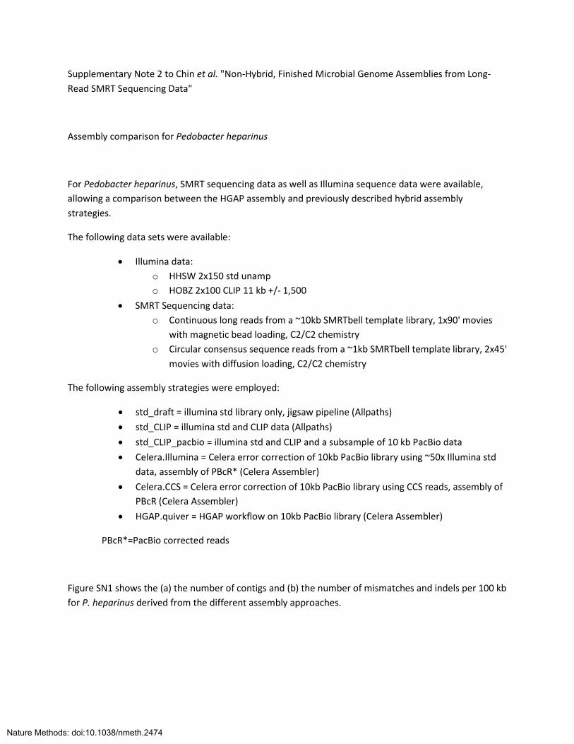
Supplementary Note 2 to Chin et al. "Non-Hybrid, Finished Microbial Genome Assemblies from Long-
Read SMRT Sequencing Data"
Assembly comparison for Pedobacter heparinus
For Pedobacter heparinus, SMRT sequencing data as well as Illumina sequence data were available,
allowing a comparison between the HGAP assembly and previously described hybrid assembly
strategies.
The following data sets were available:
Illumina data:
o HHSW 2x150 std unamp
o HOBZ 2x100 CLIP 11 kb +/- 1,500
SMRT Sequencing data:
o Continuous long reads from a ~10kb SMRTbell template library, 1x90' movies
with magnetic bead loading, C2/C2 chemistry
o Circular consensus sequence reads from a ~1kb SMRTbell template library, 2x45'
movies with diffusion loading, C2/C2 chemistry
The following assembly strategies were employed:
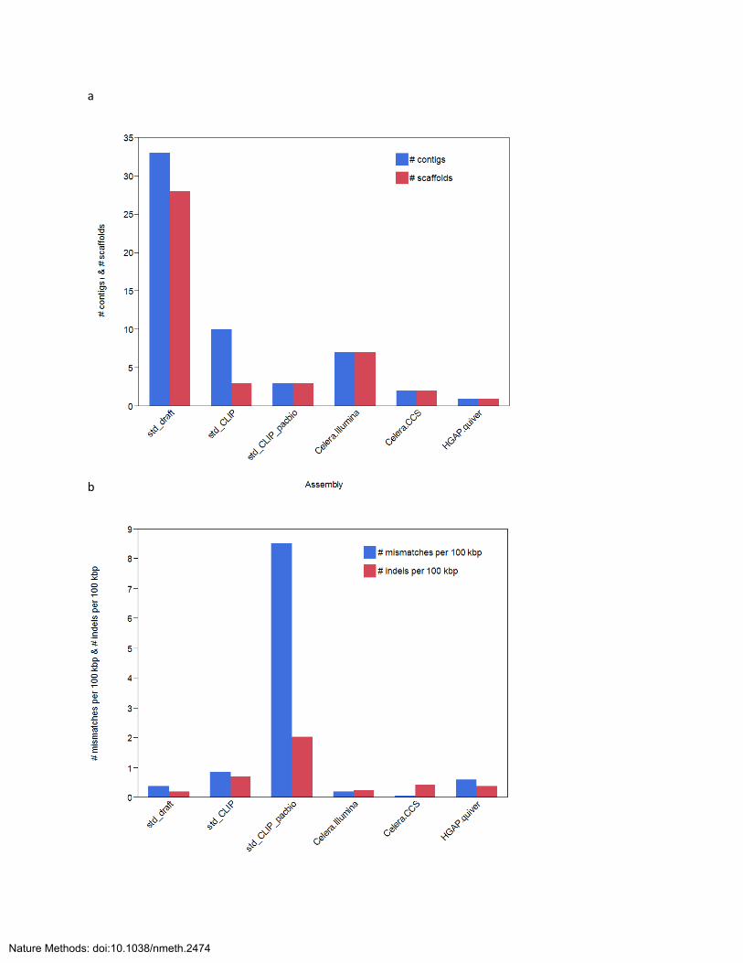
std_draft = illumina std library only, jigsaw pipeline (Allpaths)
std_CLIP = illumina std and CLIP data (Allpaths)
std_CLIP_pacbio = illumina std and CLIP and a subsample of 10 kb PacBio data
Celera.Illumina = Celera error correction of 10kb PacBio library using ~50x Illumina std
data, assembly of PBcR* (Celera Assembler)
Celera.CCS = Celera error correction of 10kb PacBio library using CCS reads, assembly of
PBcR (Celera Assembler)
HGAP.quiver = HGAP workflow on 10kb PacBio library (Celera Assembler)
PBcR*=PacBio corrected reads
Figure SN1 shows the (a) the number of contigs and (b) the number of mismatches and indels per 100 kb
for P. heparinus derived from the different assembly approaches.
Nature Methods: doi:10.1038/nmeth.2474
a
b
Nature Methods: doi:10.1038/nmeth.2474