superconducting proximity e ect in magnetic molecules · the ferromagnetic lead suppresses the...
TRANSCRIPT

Superconducting Proximity Effect
in Magnetic Molecules
By
Lina Jaurigue
A thesis
submitted to the Victoria University of Wellington
in fulfilment of the requirements for the degree of
Master of Science
Victoria University of Wellington
2013

II
III
Abstract
We studied the transport through magnetic molecules (MM) coupled to supercon-
ducting (S), ferromagnetic (F) and normal (N) leads, with the aim of investigating the
interplay between the magnetism and the superconducting proximity effect. The mag-
netic molecules were modeled using the Anderson model with an exchange coupling
between the electron spins and the spin of the molecule. We worked in the infinite
superconducting gap limit and treated the coupling between the molecule and the su-
perconducting lead exactly, via an effective Hamiltonian. For the F/N-MM-S systems
we used a real-time diagrammatic perturbation theory to calculate the electronic trans-
port properties of the systems to first order in the tunnel coupling to the normal or
ferromagnetic lead and then analysed the properties with respect to the parameters of
these models. For these systems we found that the current maps out the excitation
energies of the eigenstates of the effective Hamiltonian and that various parameters
in these systems can lead to a negative differential conductance. In the N-MM-S case
the current had no overall spin dependence, but when the normal lead is instead fer-
romagnetic there was a spin dependence and both the electronic and molecular spin
expectation values could take on non-zero values. We also found that the polarisation of
the ferromagnetic lead suppresses the superconducting proximity effect. Furthermore
in the N-MM-S case the Fano factor indicated a transition from Poissonian transport
of single electrons to Poissonian transport of electron pairs as the superconducting
proximity effect goes out of resonance, however in the F-MM-S case this did not occur.
For the S-MM-S systems we calculated the equilibrium Josephson current and found
that in the infinite superconducting gap limit no 0 − π transition was possible. Ad-
vantages of this study compared to related ones are that we allow for arbitrarily large
Coulomb interactions and we take into account coupling to the superconducting lead
non-perturbatively. This is however at the expense of working in the superconducting
gap limit. Recently it has been possible to couple single molecules to superconducting
leads. This study therefore aims to be indicative of the transport properties that will
be observed in future experiments involving single magnetic molecules coupled to leads.

IV
Acknowledgements
I thank my supervisor Michele for all he has taught me and for all the questions he has
answered.
I thank Victoria University and the MacDiarmid Institute for financial support.
I thank Stephan Meyer and Walter Somerville for helping me with Latex.
I thank Stephanie Droste for discussions.
I thank Jonnel for his support.
Contents
1 Introduction 2
1.1 Magnetic Molecules . . . . . . . . . . . . . . . . . . . . . . . . . . . . . 4
1.1.1 Anderson Model . . . . . . . . . . . . . . . . . . . . . . . . . . 5
1.1.2 Quantum Dots . . . . . . . . . . . . . . . . . . . . . . . . . . . 6
1.2 Superconductivity, AB States and the Josephson Effect . . . . . . . . . 7
1.2.1 BCS Theory . . . . . . . . . . . . . . . . . . . . . . . . . . . . . 8
1.2.2 Andreev Reflection . . . . . . . . . . . . . . . . . . . . . . . . . 10
1.2.3 Josephson Current . . . . . . . . . . . . . . . . . . . . . . . . . 11
1.3 Electronic Transport Through Molecules and QDs . . . . . . . . . . . . 12
1.4 Outline . . . . . . . . . . . . . . . . . . . . . . . . . . . . . . . . . . . . 17
2 Real-time Keldsyh Diagram Expansion 19
2.1 Master Equation . . . . . . . . . . . . . . . . . . . . . . . . . . . . . . 20
2.2 Current . . . . . . . . . . . . . . . . . . . . . . . . . . . . . . . . . . . 25
2.3 Full Counting Statistics . . . . . . . . . . . . . . . . . . . . . . . . . . . 26
3 IMM Coupled to Normal and BCS Leads 29
3.1 N-IMM-S System . . . . . . . . . . . . . . . . . . . . . . . . . . . . . . 30
3.1.1 Effective Hamiltonian . . . . . . . . . . . . . . . . . . . . . . . . 33
3.2 Transition Rates and Current . . . . . . . . . . . . . . . . . . . . . . . 37
3.3 Results . . . . . . . . . . . . . . . . . . . . . . . . . . . . . . . . . . . . 40
3.3.1 Equilibrium and Zero Exchange Coupling Limits . . . . . . . . . 40
3.3.2 Andreev Current . . . . . . . . . . . . . . . . . . . . . . . . . . 41
3.3.3 Fano Factor . . . . . . . . . . . . . . . . . . . . . . . . . . . . . 46
3.4 N-IMM-S Conclusions . . . . . . . . . . . . . . . . . . . . . . . . . . . 47
4 AMM Coupled to Normal and BCS Leads 49
4.1 N-AMM-S System . . . . . . . . . . . . . . . . . . . . . . . . . . . . . 49
V

CONTENTS 1
4.2 Transition Rates and Current . . . . . . . . . . . . . . . . . . . . . . . 52
4.3 Results . . . . . . . . . . . . . . . . . . . . . . . . . . . . . . . . . . . . 53
4.4 N-AMM-S Conclusions . . . . . . . . . . . . . . . . . . . . . . . . . . . 55
5 Josephson Current 59
5.1 S-MM-S Systems . . . . . . . . . . . . . . . . . . . . . . . . . . . . . . 59
5.2 Current . . . . . . . . . . . . . . . . . . . . . . . . . . . . . . . . . . . 61
5.3 Results . . . . . . . . . . . . . . . . . . . . . . . . . . . . . . . . . . . . 62
5.4 Josephson Current Conclusions . . . . . . . . . . . . . . . . . . . . . . 65
6 IMM Coupled to Ferromagnetic and BCS Leads 67
6.1 F-IMM-S System . . . . . . . . . . . . . . . . . . . . . . . . . . . . . . 68
6.2 Transition Rates and Current . . . . . . . . . . . . . . . . . . . . . . . 71
6.2.1 Collinear . . . . . . . . . . . . . . . . . . . . . . . . . . . . . . . 72
6.2.2 Non-collinear . . . . . . . . . . . . . . . . . . . . . . . . . . . . 73
6.3 Results - Collinear . . . . . . . . . . . . . . . . . . . . . . . . . . . . . 77
6.3.1 Ferromagnetic Lead, B=0 . . . . . . . . . . . . . . . . . . . . . 77
6.3.2 External Magnetic Field, P=0 . . . . . . . . . . . . . . . . . . . 85
6.3.3 Ferromagnetic Lead and External Magnetic Field . . . . . . . . 89
6.4 Results - Non-collinear . . . . . . . . . . . . . . . . . . . . . . . . . . . 90
6.4.1 Dependence of Current on ΓF . . . . . . . . . . . . . . . . . . . 91
6.4.2 Effect of Polarisation and Alignment of the Magnetisation of the
Ferromagnetic Lead - B= ΓS = 2J . . . . . . . . . . . . . . . . . 93
6.4.3 Varying J , B and ΓS, and the Effect of Shifting the Off Diagonal
Reduced Density Matrix Element Resonances . . . . . . . . . . 102
6.5 F-IMM-S Conclusions . . . . . . . . . . . . . . . . . . . . . . . . . . . . 105
7 Summary and Conclusions 107
Appendix
A Diagrammatic Rules 109
B Eigenstates of the AMM-S System 111
C Generalised Transition Rates – F-IMM-S 115
C.1 Solving Integrals of Generalised Transition Rates . . . . . . . . . . . . 115
C.2 Generalised Transition Rates . . . . . . . . . . . . . . . . . . . . . . . . 118

Chapter 1
Introduction
As semi-conductor based electronics are reaching their limits there are exciting new
possibilities on the horizon. In 1994 Peter Shor showed that a quantum algorithm
could exponentially speed up classical computations [1]. Since then researchers around
the globe have been working towards the realisation of quantum computing. The
fields of spintronics, nano-electronics and molecular electronics play an essential role
in achieving this goal, as it is through the manipulation of individual spins, electrons
and atoms that devices capable of quantum computing will be made.
Single molecule magnets (SMM) have received a lot attention in the past few years
as they are a good platform for developing devices which exhibit spin dependent trans-
port and could therefore be used for quantum information storage and processing [2]. A
significant amount of research has been carried out on the transport properties through
systems containing quantum dots [3–7]. In comparison the research done on electronic
and spin transport through magnetic molecules is still in its early stages. Furthermore,
it is only through recent advances in nano-fabrication techniques that experimentalists
are now capable of contacting individual molecules to electrodes [8–13].
As with quantum dots, due to the size and relatively few degrees of freedom of
an individual molecule, quantisation and charging effects play an important role in
transport. To realise transport through molecules they are coupled to leads. Depend-
ing on the type of leads different effects can be observed. Experimental work on C60
molecules between superconducting leads has exhibited Josephson currents [14], Kondo
correlations [15,16] and Coulomb interaction effects [13]. Quantum dots coupled to su-
perconducting leads have been extensively studied [5,13,17,18] and it has been shown
that a superconducting proximity effect induces Andreev bound states [19] in the quan-
tum dot. As magnetism and superconductivity are competing effects it is interesting,
2

3
from not only a practical point of view but also due to the interesting physics that could
arise, to investigate the effects of coupling a magnetic molecule to a superconducting
lead. For practical applications it is interesting to investigate if such a system can
exhibit spin dependent transport, for then the extra degrees of freedom introduced by
the spin dependence can be utilised along with the coherent, dissipation-less transport
properties of the superconductor. In this thesis we will therefore perform a theoretical
study on the electronic transport properties of systems involving a magnetic molecule
coupled to a superconducting lead. For simplicity we will focus on an idealised model
for the magnetic molecule. Nevertheless, when transport is dominated by the molec-
ular orbital closest to the Fermi level of the leads this model should be predictive of
electronic transport through magnetic molecules.
Recent theoretical studies have looked at the Josephson current through isotropic
and anisotropic magnetic molecules [20,21]. In these works the models for the molecules
contained a single orbital level, an energy cost U for double occupation, which is due to
Coulomb interactions, and an exchange coupling between the electronic and molecular
spins. References [20] and [21] treated the superconducting gap ∆ as finite, however for
simplicity they let U →∞. We will be concerned with only sub-gap transport and will
therefore let ∆→∞. This will allow us to perform a non-perturbative expansion in the
tunnel coupling to the superconducting lead which will let us easily include arbitrarily
strong Coulomb interactions. Because we are interested in the effect of superconduct-
ing proximity effect on the magnetic molecule we will consider strong coupling to the
superconducting lead. In the past, experiments have been conducted on quantum dots
coupled to superconducting leads but due to technical difficulties, such as the oxida-
tion between the superconductor and semiconductor interfaces completely suppressing
Cooper pair tunneling, these setups were only in the weak coupling regime. However
the development of new materials such as carbon nanotubes and self-assembled quan-
tum dots, as well as the ability to couple single molecules to leads, has now made it
possible to carried out experiments in the intermediate to strong coupling regimes [3].
In this thesis we investigate the transport properties of the MM-S subsystem cou-
pled to normal, ferromagnetic and superconducting leads. For the case of coupling to
a ferromagnetic lead we will look at the effects of applying an external magnetic field
and will allow for arbitrary alignment of the magnetisation of the ferromagnetic lead
and the external magnetic field. To investigate the transport properties we will calcu-
late the sequential current through these systems by using a real-time diagrammatic
perturbation theory.

4 CHAPTER 1. INTRODUCTION
1.1 Magnetic Molecules
In recent years the electronic transport properties of single molecules have attracted
a lot of attention, both experimentally and theoretically [10–13, 20–22]. This is due
to advances in nano-fabrication techniques [12] as well as quantum effects, such as
tunneling, the Coulomb blockade and the Kondo effect [23], which can be observed in
these single molecules. A subset of single molecules that are of particular interest, due
to their potential application in spintronics, are molecular magnets.
Figure 1.1: Examples of SMMs. a) shows Mn12 [21], b) shows Fe8 [10] and c) showsN@C60 [11].
A conventional magnet is usually made of some ferromagnetic metal in which the
spins of the electrons are aligned and a macroscopic number of coupled centers are
involved. A single molecule magnet (SMM) is very different from a conventional magnet
due to the small number of coupled centers and the structure of the molecule; they are
strictly speaking not magnets as they are not in the thermodynamic limit. An SMM
is defined as a molecule whose magnetization is persistent over long time scales. An
example is Mn12 acetate which has a relaxation of magnetisation of the order of months
at a temperature of 2 K [24].
The prototypical SMM is Mn12 acetate (Mn12). This molecule consists of organic
ligands bonded to 12 manganese ions. There are various derivatives of Mn12 which
feature different ligands, one example is [Mn12O12(O2C-C6H4-SAc)16(H2O)] [12]. Fig-
ure 1.1 a) shows a schematic diagram of an Mn12 molecule. The total spin of Mn12
is S= 10 and the molecule has an anisotropy barrier of about 6 meV [25]. Due to the
large spin and high anisotropy barrier molecules such as Mn12 show magnetic hystere-
sis. The high anisotropy barrier is important in achieving long relaxation times of the

1.1. MAGNETIC MOLECULES 5
magnetisation of the molecule. Also shown in Fig. 1.1 are diagrams of the structures
of Fe8 and N@C60. Fe8 is another SMM that has received a lot of attention [10]. The
formula for this molecule is [Fe8O2(OH)12(tacn)6]Br8 (tacn = 1,4,7-triazacyclononane),
it also has total spin S= 10. For Fe8 the relaxation times becomes long enough to per-
form direct measurements at temperatures under 1 K [26]. The third molecule, N@C60,
is a nitrogen atom caged in a C60 molecule. The total spin S=3/2 of this molecule is
much lower than the previously mentioned molecules [11]. Within the C60 cage much
of the atomic character of the nitrogen atom is retained, which is often not the case
since previous studies involving SMMs have shown that strong interaction with the
environment can destroy the molecular magnetism [27]. Due to this there is interest in
using the nuclear spin of the nitrogen atom or the electron spin residing on the atom
for quantum information processing [2].
SMMs typically have quite a complicated structure (Fig. 1.1). To theoretically
model such molecules is very difficult, therefore for general studies on the transport
properties of magnetic molecules simplifying approximations are usually made. To
reduce the degrees of freedom of the molecule, often only one orbital level is considered
[20–23]. This approximation is realistic in a scenario where the spacing between orbital
levels is large enough such that only one level is accessible in the energy regime of
interest. In this case the model for describing the molecule coupled to leads is based
on the Anderson model. The Anderson model was first developed by P. W. Anderson
to model localised magnetic states in metals [28] and has since been widely used to
model quantum dots and magnetic molecules. The Anderson model is described in the
next subsection.
1.1.1 Anderson Model
Here we give the Anderson model describing a single orbital level coupled to two metal-
lic systems. The Hamiltonian reads
HD =∑σ
εd+σ dσ + Un↑n↓, (1.1)
where d(+)σ is an electron annihilation (creation) operator, nσ = d+
σ dσ is the number
operator and σ =↑, ↓ is the spin of the electron. The first term describes the occupation
of the level, it can either be empty, singly occupied, or doubly occupied. The second
term is the Coulomb interaction term, it describes the energy cost of double occupation,
U .

6 CHAPTER 1. INTRODUCTION
To describe the tunneling coupling to the leads the Hamiltonian
Htunn,η =∑k,σ
(VηkσC+ηkσdσ +H.c.) (1.2)
is used. Here C+ηkσ is the electron creation operator for lead η = L,R and Vηkσ is the
tunneling matrix element, which is related to the strength of the coupling. The leads
are treated as equilibrium reservoirs and in the case of normal metallic leads they can
be modeled by
Hη =∑k,σ
εkC+ηkσCηkσ. (1.3)
This simple model is usually employed to describe transport through quantum dots
but can easily be modified to include effects that occur in magnetic molecules. Such
effects include exchange coupling between electronic and molecular spins, anisotropy,
and quantum tunneling of magnetisation. The Hamiltonians describing the leads can
also be modified to describe ferromagnetic or superconducting leads.
1.1.2 Quantum Dots
As the model for describing a single orbital magnetic molecule reduces to that of a
quantum dot in certain limits, it can be useful to compare the transport properties of
these systems. We therefore give a brief introduction to quantum dots in this section.
Quantum dots are made by confining the charge carriers to a small region in a
semi-conducting material in all three spatial directions. They contain 103-109 atoms
and range in size from several nanometers to microns [29]. Due to their size, their
properties are intermediate between bulk semiconductors and atoms and have been
referred to as artificial atoms [30]. Striking properties of quantum dots are that both
the charge on and the energy of the dot are quantised. Like atoms, quantum dots have
well defined energy levels, yet unlike in atoms the level spacing can be tuned. It is this
control that makes quantum dots so attractive for a wide range of applications in fields
including optics [31], nano-electronics [4] and quantum computing [32–34].
Properties of quantum dots can be investigated by performing electronic transport
measurements. To do this the quantum dot is contacted to source and drain electrodes.
Figure 1.2 shows a schematic diagram of such a setup. As well as being contacted to
the electrodes the quantum dot is also capacitively coupled to a gate. Varying the
gate voltage will shift the orbital levels of the quantum dot, thereby controlling which
levels are in the energy regime needed for transport. Due to the size of the quantum

1.2. SUPERCONDUCTIVITY, AB STATES AND THE JOSEPHSON EFFECT 7
dot Coulomb repulsion effects are strong. For an electron to tunnel onto the dot
it must have enough energy to overcome the repulsion due to the electrons already
occupying the dot. This is energy, referred as the charging energy, is dependent on the
gate voltage. Therefore tuning the gate voltage can control when sequential tunneling
can occur and when the system is in the so called Coulomb blockaded regime where
transport is forbidden.
Figure 1.2: a) Schematic diagram of a quantum dot. The boxes represent the tunnelbarriers. b) Scanning electron microscope image of a lateral quantum dot [35].
1.2 Superconductivity, Andreev Bound States and
the Josephson Effect
Superconductivity is a very well-researched phenomenon that was discovered by Heike
Kamerlingh Onnes in 1911 [36]. A material in the superconducting state has zero
electrical resistance and zero magnetic field in its interior. The exclusion of magnetic
field was discovered by Meissner and Ochsenfeld in 1933 and is known as the Meissner
effect [37]. Since its discovery much work has been carried out to theoretically describe
superconductivity. The first successful microscopic theory of superconductivity was de-
veloped by Bardeen, Cooper and Schrieffer [38], the so call BCS theory. In BCS theory
it was shown that electrons could form pairs in the presence of just a weak attractive
interaction to form a new ground state. The effective interaction is often provided
by an electron-phonon interaction. The bound electrons are called Cooper pairs; they
have equal and opposite momenta, so that the ground state has zero momentum. To
calculate the ground state wavefunction BCS used a mean field approach to describe
the dependence of the occupation of one state on all other states. Through this they
8 CHAPTER 1. INTRODUCTION
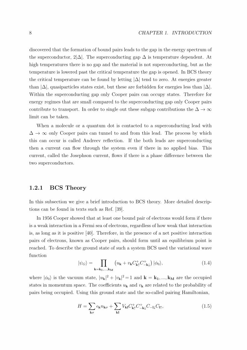
discovered that the formation of bound pairs leads to the gap in the energy spectrum of
the superconductor, 2|∆|. The superconducting gap ∆ is temperature dependent. At
high temperatures there is no gap and the material is not superconducting, but as the
temperature is lowered past the critical temperature the gap is opened. In BCS theory
the critical temperature can be found by letting |∆| tend to zero. At energies greater
than |∆|, quasiparticles states exist, but these are forbidden for energies less than |∆|.Within the superconducting gap only Cooper pairs can occupy states. Therefore for
energy regimes that are small compared to the superconducting gap only Cooper pairs
contribute to transport. In order to single out these subgap contributions the ∆→∞limit can be taken.
When a molecule or a quantum dot is contacted to a superconducting lead with
∆ → ∞ only Cooper pairs can tunnel to and from this lead. The process by which
this can occur is called Andreev reflection. If the both leads are superconducting
then a current can flow through the system even if there in no applied bias. This
current, called the Josephson current, flows if there is a phase difference between the
two superconductors.
1.2.1 BCS Theory
In this subsection we give a brief introduction to BCS theory. More detailed descrip-
tions can be found in texts such as Ref. [39].
In 1956 Cooper showed that at least one bound pair of electrons would form if there
is a weak interaction in a Fermi sea of electrons, regardless of how weak that interaction
is, as long as it is positive [40]. Therefore, in the presence of a net positive interaction
pairs of electrons, known as Cooper pairs, should form until an equilibrium point is
reached. To describe the ground state of such a system BCS used the variational wave
function
|ψG〉 =∏
k=k1,...,kM
(uk + vkC
+k↑C
+−k↓)|φ0〉, (1.4)
where |φ0〉 is the vacuum state, |uk|2 + |vk|2 = 1 and k = k1, ...,kM are the occupied
states in momentum space. The coefficients uk and vk are related to the probability of
pairs being occupied. Using this ground state and the so-called pairing Hamiltonian,
H =∑kσ
εknkσ +∑kl
VklC+k↑C
+−k↓C−l↓Cl↑, (1.5)

1.2. SUPERCONDUCTIVITY, AB STATES AND THE JOSEPHSON EFFECT 9
the coefficients uk and vk can be calculated. These are found to be
|vk|2 =1
2
(1− ξk
Ek
)(1.6)
and
|uk|2 =1
2
(1 +
ξkEk
), (1.7)
where ξk = εk − µS is the is single particle energy εk relative to the Fermi level µS,
Ek = (∆2 + ξ2k)
1/2and ∆ is related to the pairing potential Vkl which is chosen to be
−V for states below a cut-off energy ~ωc and zero otherwise. In Ginzburg-Landau
theory for superconductivity ∆ is the order parameter and contains a phase factor eiϕ,
where ϕ is the phase difference between uk and vk. This leads to the BCS mean field
Hamiltonian
HS =∑kσ
(εk − µS)C+kσCkσ −∆
∑k
(C−k↓Ck↑ + C+k↑C
+−k↓). (1.8)
for an s-wave superconductor. This Hamiltonian does not conserve particle number, but
for the purposes of this work this does not matter since we treat the superconducting
lead as an equilibrium reservoir with a fix electrochemical potential. HS is quadratic
in electron operators and can therefore be diagonalised. To do this the Bogoliubov
quasi-particle operators
γk↑ ≡ ukck↑ − vkc+−k↓, (1.9)
γk↓ ≡ ukck↓ + vkc+−k↑. (1.10)
are introduced. The creation operators are the Hermitian conjugates. Using these
fermionic quasi-particle operators, with the definitions of uk and vk given above, ne-
glecting an irrelevant constant the BCS Hamiltonian can be cast into the form
HS =∑kσ
Ekγ+kσγkσ, (1.11)
where Ek has the same definition as above and has turned out to be the quasi-particle
excitation energy. From the equation for Ek we can see that ∆ is half the width of the
gap in the single particle density of states of the superconductor, as |∆| is the minimum
energy a quasi-particle can have. Figure 1.3 shows the quasi-particle density of states
of a superconductor. For energies less than |∆| either side of the Fermi level there are
no single particle states; in this energy range only Cooper pairs are allowed.

10 CHAPTER 1. INTRODUCTION
Figure 1.3: The single particles density of states for a superconductor, NS, showsa symmetric gap about µS with a width of 2|∆|. Out side the gap quasi-particleexcitations are possible, however at energies inside the gap only Cooper pairs areallowed.
1.2.2 Andreev Reflection
When a normal metal is contacted to a superconductor then superconductivity can
be induced in the normal metal. This is known as the proximity effect [41] and has
been known of since the 1930s [42]. If the Fermi level of the metal lies within the
gap of the superconductor then a single electron cannot enter the superconductor from
the metal as there are no available states. Therefore if an electron is incident on the
boundary between the metal and the superconductor it must be reflected (Fig. 1.4).
This electron can be reflected in the form of a hole with the opposite velocity of the
incident electron and the opposite spin. This means that both momentum and spin are
conserved in this reflection process. In this process a Cooper pair is transferred into the
superconductor, which makes up for the charge 2e that is lost in the reflection process.
This process is called Andreev reflection [43, 44] and is a convenient way to explain
the process by which a Cooper pair can pass between the two materials. When the
normal metal is in between two superconducting leads then the hole that is reflected
from one boundary must be reflected as an electron from the opposite boundary. This
process happens repeatedly and can lead to constructive interference of the incident
and reflected electron waves, forming a so called Andreev bound state [19].
If there is a molecule or a quantum dot contacted to a superconducting lead then
the same process occurs. However in this case it is the orbital levels of the molecule or
quantum dot that are relevant, rather than the Fermi level of the metal.
1.2. SUPERCONDUCTIVITY, AB STATES AND THE JOSEPHSON EFFECT 11
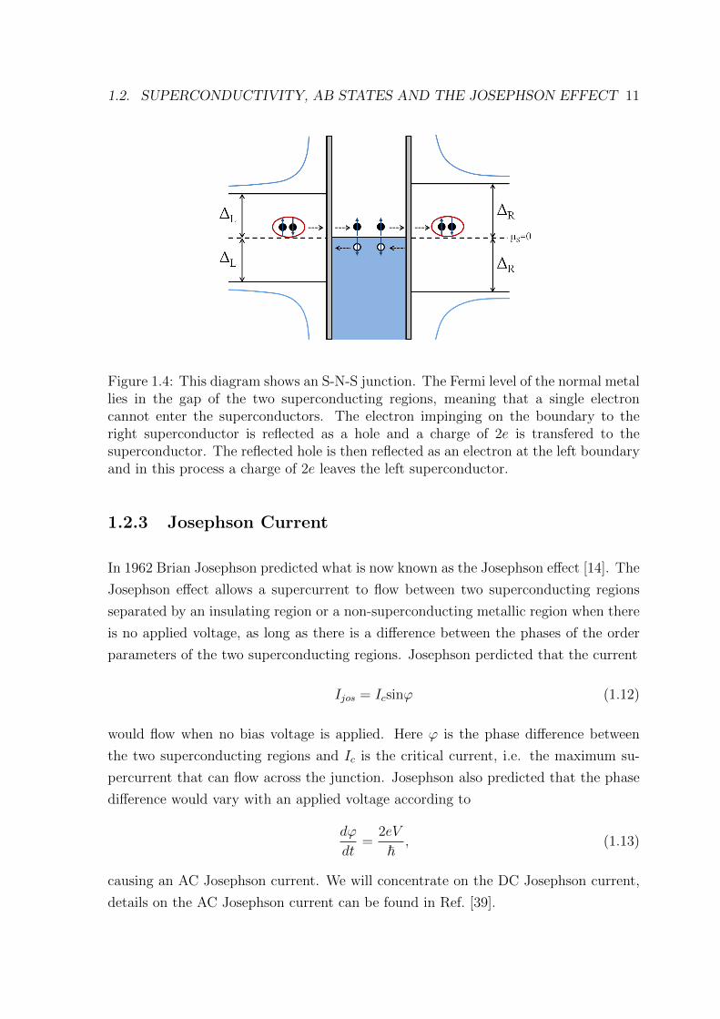
Figure 1.4: This diagram shows an S-N-S junction. The Fermi level of the normal metallies in the gap of the two superconducting regions, meaning that a single electroncannot enter the superconductors. The electron impinging on the boundary to theright superconductor is reflected as a hole and a charge of 2e is transfered to thesuperconductor. The reflected hole is then reflected as an electron at the left boundaryand in this process a charge of 2e leaves the left superconductor.
1.2.3 Josephson Current
In 1962 Brian Josephson predicted what is now known as the Josephson effect [14]. The
Josephson effect allows a supercurrent to flow between two superconducting regions
separated by an insulating region or a non-superconducting metallic region when there
is no applied voltage, as long as there is a difference between the phases of the order
parameters of the two superconducting regions. Josephson perdicted that the current
Ijos = Icsinϕ (1.12)
would flow when no bias voltage is applied. Here ϕ is the phase difference between
the two superconducting regions and Ic is the critical current, i.e. the maximum su-
percurrent that can flow across the junction. Josephson also predicted that the phase
difference would vary with an applied voltage according to
dϕ
dt=
2eV
~, (1.13)
causing an AC Josephson current. We will concentrate on the DC Josephson current,
details on the AC Josephson current can be found in Ref. [39].

12 CHAPTER 1. INTRODUCTION
The electrical work done by the current source is
W = F =
∫IjosV dt =
∫Ijos
~2edϕ, (1.14)
where F is the free energy stored in the junction. Rearranging this equation we find
Ijos = −2e
~∂F
∂φ. (1.15)
If the states of the system in question are discrete then the free energy can be calculated
using
F = −kBT lnZ, (1.16)
where
Z =∑i
e− EikBT (1.17)
is the partition function and Ei is the energy of state i. Substituting the free energy
and the partition function into Eq. 1.15, the Josephson current can be expressed as
Ijos =2e
~kBT
∂
∂φlnZ = −2e
~∑i
∂Ei∂φ
e− EikBT
Z. (1.18)
The critical current in Eq. 1.12 can be positive or negative. When Ic> 0 the Joseph-
son phase ϕ of the junction is zero in the ground state (when no current is flowing).
When Ic< 0 Eq. 1.12 can be rewritten as
Ijos = −|Ic|sinϕ = |Ic|sin (ϕ+ π) . (1.19)
Here we see that ϕ=π when Ijos = 0. When this is the case the junction is said to
be a π-Josephson junction. Under certain circumstances a Josephson junction can
transition between the zero and π phases.
1.3 Electronic Transport Through Molecules and
Quantum Dots
In this section we will address how electronic transport through molecules and quantum
dots is realised. We will then review some of the relevant experimental and theoretical
work that has be done in the fields of nano and molecular electronics.

1.3. ELECTRONIC TRANSPORT THROUGH MOLECULES AND QDS 13
Figure 1.5: A molecule coupled to a normal metal lead and a superconducting lead.The blue lines in the central region indicate the orbital levels of the molecule. Thestates of the molecule that contribute to the current are those that lie within the biaswindow set by the two leads.
To study the electronic transport properties through a molecule (or a quantum dot)
it must be contacted to at least two conducting leads. These leads can be supercon-
ducting, magnetic or normal metallic. In each case, for current to flow the energy levels
of the molecule must lie within the bias window set by the leads. Figure 1.5 shows
a schematic diagram of a molecule weakly coupled to a normal metallic lead on the
left and strongly coupled to a superconducting lead on the right. The levels of the
molecule lie within the gap of the superconductor, meaning that no single particles
can tunnel between the superconducting lead and the molecule. In an experimental
setup the energy levels of the molecule could be tuned by applying a gate voltage.
The choice of material for the leads depends on the effects to be investigated. With
superconducting leads interesting effects include the proximity, Josephson, and Kondo
effects. Ferromagnetic leads can cause spin-dependent transport, spin accumulation on
the molecule and a ferromagnetic proximity effect. Some of these effects can be used
to probe properties of the molecule through which transport is occurring [45] [46] [20].
Systems which contain a combination of lead types are also of interest for pure physics
reasons, and for the possibility of developing devices with new properties which could
be useful in areas such as spintronics, quantum computing and optics.
In this thesis we investigate the transport properties of a magnetic molecule coupled
to a superconducting lead and a second lead which can either be a normal metal,

14 CHAPTER 1. INTRODUCTION
ferromagnetic or superconducting. For the remainder of this section we will review
some of the theoretical and experimental research that has been carried out on systems
containing combinations of the aforementioned components.
Most experimental work that has been carried out on SMMs has involved normal
metallic leads, gold is commonly used. Heersche et al. have performed transport mea-
surements through a single Mn12 molecule coupled to gold electrodes. They observed
negative differential conductance features on the energy scale of the anisotropy barrier,
something they had not previously observed with other molecules or bare gold samples.
Figure 1.6 shows an SEM image of the type of devices they have tested. The molecule
is too small to be resolved but it sits in the gap between the two gold electrodes. Heer-
sche et al. found that with a simple model that incorporates the anisotropy of the
molecule and the quantum tunneling of magnetisation they were able to qualitatively
understand current and differential conductance features in the sequential tunneling
regime [12]. The current calculations we will perform in this work will also be in the
sequential tunneling limit for coupling to a normal lead. Roch et al. have carried out
experimental and theoretical studies on N@C60 coupled to gold electrodes. They calcu-
lated the current in both the sequential tunneling regime and the cotunneling regime.
In both cases they found good qualitative agreement between their experimental and
their theoretical results and that an anti-ferromagnetic exchange between the nitrogen
atom and the C60 molecule best fits the data [11].
Figure 1.6: A scanning electron microscope (SEM) image of a Mn12 molecule contactedto two gold electrodes. The scale bar corresponds to 200 nm and the width of themolecule is about 3 nm [12].
Zyazin et al. carried out measurements on individual Fe4 SSMs. They coupled the
molecule to three gold electrodes to perform three-terminal transport measurements
in the presence of an external magnetic field. The ground states spin of Fe4 is S=5
and this is retained when the molecule is deposited on gold. Using the transport

1.3. ELECTRONIC TRANSPORT THROUGH MOLECULES AND QDS 15
measurements they were able to make estimates of the easy axis anisotropy constant
and the anisotropy barrier of the molecule and demonstrated that, via an electric field,
they could control the anisotropy of an SMM [9]. The ability to control properties of
SMMs is important for their use in applications such as quantum computing. Parks et
al. have also reported the experimental confirmation of mechanical control of the spin
states and anisotropy of a SMM; in this case a Cobalt complex [8].
The experimental work discussed so far has involved only normal metallic leads.
We will now discuss two experimental studies that involve superconducting and fer-
romagnetic leads, neither of these studies however involve SMMs. Winkelmann et al.
have carried out electronic transport measurements on C60 molecules coupled to su-
perconducting leads. The superconducting leads are made of either aluminium or gold
in the proximity of an aluminium capping layer. They engineered samples with weak
to strong coupling to the leads and demonstrated the coexistence and competition of
superconductivity and Kondo correlations for varying coupling strength and external
magnetic field magnitudes [13]. This work paves the way for similar experiments in-
volving endofullerenes such as N@C60. The second study was carried out by Hofstetter
et al.. They studied the ferromagnetic proximity effect in a quantum dot coupled to
a superconducting and a ferromagnetic lead. Figure 1.7 shows an image of a typical
devices they have constructed. Through transports measurements they were able to
demonstrate that a local exchange field is induced in the quantum dot due to the fer-
romagnetic lead. They used the Kondo effect to probe the local exchange field. With
respect to the energy regime they were working in the superconducting lead had a finite
gap [45].
A lot of theoretical research has has been carried out on electronic transport through
quantum dots. Sothmann et al. studied the transport properties of a quantum dot
coupled to two ferromagnetic leads and one superconducting lead. They worked in
the infinite superconducting gap limit, considered a finite Coulomb interaction and
allowed for arbitrary alignment of the ferromagnetic leads. The F-QD-F subsystem
forms a quantum dot spin valve, a device that has received a lot of experimental and
theoretical interest due to the spin dependence of electronic transport through this
system. They were able show that by introducing the superconducting lead the ex-
change field induced by the proximity to the ferromagnetic lead could be experimentally
probed [46]. Sothmann et al. have used the same real-time diagrammatic technique
that we use in this thesis. The same diagrammatic approach is used in [5] and [47] to
calculate the current through quantum dots coupled to normal and superconducting

16 CHAPTER 1. INTRODUCTION
Figure 1.7: A SEM image of an InAs nanowire contacted to a Ti/Al bilayer supercon-ducting lead and a Ni/Co/Pd trilayer ferromagnetic lead, with an external magneticfield applied parallel to the easy axis of the ferromagnetic lead [45].
leads. Governale et al. model an interacting quantum dot coupled to a normal and
two superconducting leads. In the infinite superconducting gap limit they found that
there is a π transition in the non-equilibrium Josephson current, which can be triggered
by both the voltage of the normal lead and the gate voltage, which controls the level
position [5]. Braggio et al. performed a theoretical study on an interacting quantum
dot coupled to a normal metallic lead and a superconducting lead. They also worked
in the limits of infinite superconducting gap and finite Coulomb interaction. To study
the superconducting proximity effect in this system they used full counting statistics
to obtain the current and the zero frequency noise. They found that the Fano factor
changes from 2 to 1 as the superconducting proximity effect goes from off-resonance to
resonance conditions. This suggests Poissonian transport in both regimes, one electron
transport on resonance as the transport is limited by single electron tunneling events
between the dot and the normal lead, and two electron transport off resonance as in
this regime the current is limited by the tunneling of electron pairs to and from the
superconducting lead [47]. In the limit of zero exchange coupling between the elec-
tronic and molecular spins the dynamics of the single level isotropic magnetic molecule
(IMM) in an N-IMM-S system reduce to those of the systems studied in [5] and [47].
In the theoretical work of Lee et al. the Josephson effect through an isotropic
magnetic molecule is investigated. They work with a finite superconducting gap and

1.4. OUTLINE 17
model the magnetic molecule as a single level quantum dot with an exchange interaction
between molecular spin and the electron spin. They use a numerical renormalisation
approach to calculate non-perturbative low temperature transport properties. To do
this they work in the regime of infinite Coulomb interaction between electrons on the
molecule, meaning that the level of the molecule can only be singly occupied or empty.
They find that when the superconducting gap exceeds the Kondo temperature the
Josephson junction is in the π state, however with sufficiently large antiferromagnetic
exchange coupling the 0 state is restored. Due to the asymmetry in the behaviour
with the exchange coupling Lee et al. suggest that the sign of the coupling could be
determined experimentally [20]. In this thesis we use the same model for the isotropic
magnetic molecule as is used by Lee et al. However we work in a different regime. As
we will work in the ∆ → ∞ limit transport will only be possible through Andreev
reflection processes. On the other hand, in the work of Lee et al. transport must
occur in the cotunneling regime. The results of the for the two regimes will therefore
be quite different. Sadovskyy et al. have studied a similar system to that in [20],
however their system is generalised to an anisotropic magnetic molecule. The model
they used consisted of a single level magnetic molecule in the presence of an external
magnetic field, coupled to two finite gap superconducting leads. They also worked
in the infinite Coulomb interaction limit. They used a perturbation expansion in
the tunnel coupling to the leads to calculate the Josephson current and also found
that with anti-ferromagnetic coupling between the electronic and molecular spins a π-0
transition can be induced. They also find that it is possible to obtain information of the
anisotropy of the molecule by studying the critical current [21]. Other studies involving
SMMs demonstrate that a transport spectroscopy of a SMM coupled to normal and/or
ferromagnetic leads shows signs of quantum tunneling [48] and negative differential
conductance features [22].
1.4 Outline
The aim of thesis is to investigate the electronic transport properties through systems
comprised of a magnetic molecule coupled to a superconducting lead and a second lead
that can be normal, ferromagnetic or superconducting, with the purpose of adding
new knowledge to the fields of nano and molecular electronics. To calculate the non-
equilibrium sequential current through these systems we will use a real-time diagram-
matic approach and work in the ∆ → ∞ limit. We will work in the regime of strong

18 CHAPTER 1. INTRODUCTION
coupling to the superconducting leads and weak coupling to the normal or ferromag-
netic leads. The coupling to the superconducting leads will be treated exactly by using
an effective Hamiltonian. Our main focus will be on the Andreev current but we will
also calculate the zero frequency noise and briefly look at the Josephson current in the
case where the molecules are coupled to two superconducting leads.
In Chapter 2 we introduce the diagrammatic perturbation theory that will be used
in the subsequent chapters. In this chapter we also introduce full counting statistics
and explain how the zero frequency noise and the Fano factor can be calculated. Next,
in Chapter 3 we investigate an isotropic magnetic molecule coupled to a normal and a
superconducting lead. The spin of the molecule is incorporated into the model via an
exchange interaction between the electronic and molecular spins. We first introduce the
model then give the derivation for the effective Hamiltonian describing the coupling to
the superconducting lead. Using the eigenstates of the effective Hamiltonian we then
calculate the sequential current caused by the couping to the normal lead. In Chapter
4 we modify the system slightly to allow for the molecule to be anisotropic. Then in
Chapter 5 we use the models for the isotropic and anisotropic molecules of the pervious
two chapters and investigate the Josephson current through these molecules. Following
this, in Chapter 6 we are once again concerned with the electronic transport through
an isotropic magnetic molecule, however this time coupled to a superconducting lead
and a ferromagnetic lead in the presence of an external magnetic field. We investigate
the cases of magnetisation of the ferromagnetic lead and the external magnetic field
being collinear and non-collinear. Finally, in Chapter 7 we summaries the results of
the previous four chapters.

Chapter 2
Real-time Keldsyh Diagram
Expansion
In the following section a diagrammatic perturbation theory for a molecule, or a quan-
tum dot, with strong interactions, contacted to non-interacting leads in non-equilibrium
conditions and at finite temperature, is given. The Hamiltonian of such a system is of
the form
H = HL +HM +HT ≡ H0 +HT , (2.1)
where HL describes the leads, HM describes the molecule and HT are the tunneling
terms. The perturbation expansion that will be performed is with respect to the
tunneling Hamiltonian. The general idea of the theory is to split the density matrix of
the system into two parts, one describing the leads, which have many degrees of freedom
but are non-interacting, and the other describing the molecule, which is interacting but
has only a few degrees of freedom. Because the leads are non-interacting they can be
integrated out using Wick’s theorem, leaving the much smaller system of the molecule
to be treated exactly. The time evolution of the remaining reduced density matrix
is described by a master equation in Liouville space, the elements of which can be
calculated using diagrammatic techniques.
The advantage of this technique is that allows one to calculate non-equilibrium
dynamics, include arbitrarily strong Coulomb interactions, and easily treat off-diagonal
density matrix elements. In some cases this technique also allows non-perturbative
expansions in the tunnel coupling. This is the case with BCS leads in the ∆ → ∞limit, the expansion can be exactly summed to all orders in tunneling coupling.
The diagrammatic perturbation expansion can be used to calculate the elements of
the reduced density matrix, as well as the current. With a minor adjustment to the
19

20 CHAPTER 2. REAL-TIME KELDSYH DIAGRAM EXPANSION
theory full counting statistics can also be calculated. In this chapter we will first derive
the master equation of the reduced density matrix elements [49] then show how the
current can be calculated. Lastly, we will show how the full counting statistic can be
calculated, with an emphasis on the Fano factor.
2.1 Master Equation
The expectation value of an observable at time t is given by
〈A(t)〉 = Tr[A(t)Hρ0] (2.2)
where ρ0 is the initial density matrix of the system and AH(t) is the observable at time
t in the Heisenberg representation. We assume that at the initial time t0 the denstiy
matrix can be factorised into parts, for the molecule (or dot) ρM0 and the leads ρr0;
ρ0 = ρM0∏r=L,R
ρr0. (2.3)
The leads are treated as equilibrium reservoirs with fixed Fermi levels µr and can
therefore be described using the Fermi function f(ω) and the equilibrium density matrix
ρr0 =1
Zr0
e−β(Hr−µrNr). (2.4)
Here β = 1/kBT , where kB is the Boltzmann factor, Nr is the number operator and
Hr =∑
k,σ εkC+rkσCrkσ is the Hamiltonian that describes the leads with annihilation
(creation) operators C(+)rσ and energies εk. In the case of a superconducting lead the
Hamiltonian is that given in Eq. 1.11. The normalisation factor Zr0 is determined by
the condition Tr[ρr0] = 1. The initial density matrix describing the molecule can be
chosen to be diagonal in an appropriate basis {|χ〉} and is given by
ρM0 =∑χ
P (0)χ |χ〉〈χ|, (2.5)
where P(0)χ are the initial occupation probabilities of the states |χ〉 and
∑χ P
(0)χ = 1. We
are interested in the stationary limit, t0 → −∞. In this limit, at time t, all observables
are independent of the choice of the initial probabilities P(0)χ . Furthermore, choosing
the initial density matrix to be diagonal does not mean it must remain so at some later

2.1. MASTER EQUATION 21
time t.
Next it is useful to go from the Heisenberg picture to the interaction picture. The
aim of this section is to perform a perturbation expansion in the tunnel coupling
between the molecule and the leads, therefore we treat the tunneling Hamiltonians as
the perturbation when we change to the interaction picture. The tunneling Hamiltonian
is of the form of Eq. 1.2. Doing this gives us
A (t)H = T ei∫ tt0dt′HT (t′)IA (t)I Te
−i∫ tt0dt′HT (t′)I , (2.6)
where T (T ) is the (anti-)time ordering operator and we have set ~= 1. Substituting
this into Eq. 2.2 we get
〈A (t)〉 = Tr[T e
i∫ tt0dt′HT (t′)IA (t)I Te
−i∫ tt0dt′HT (t′)Iρ0
]. (2.7)
Reading from the right we start with ρ0 then propagate forward in time up to t, the
time at which the expectation value of A(t) is calculated, then we propagate backwards
in time back to t0. This is represented diagrammatically in Fig. 2.1. This time curve is
referred to as the Keldysh contour and propagation along this contour can be written
more compactly by introducing the Keldysh time ordering operator TK , which acts on
all operators to the right of it,
〈A(t)〉 = Tr
[TK exp
(−i∫K
dt′HT (t′)
)A(t)Iρ0
]. (2.8)
Figure 2.1: A diagrammatic representation of Eq. 2.7. Along the top path the systemis propagated forward to the time when the observable is measured, then backwardalong the bottom path to the initial time.
To calculate the elements of the reduced density matrix of the molecule P χ1χ2
(t) we
must find the expectation value of the projection operator |χ2〉〈χ1|(t). Replacing A(t)

22 CHAPTER 2. REAL-TIME KELDSYH DIAGRAM EXPANSION
in Eq. 2.8 with |χ2〉〈χ1|(t) we find
P χ1χ2
(t) = 〈|χ2〉〈χ1|(t)〉 = Tr
[TK exp
(−∫K
dt′HT (t′)I
)|χ2〉〈χ1|(t)Iρ0
]. (2.9)
Writing out the trace over the states of the molecule in terms of the sum over the states
and the using Eqs. 2.3 and 2.5, this can be written as
P χ1χ2
(t) =∑χ′1,χ
′2
〈χ′2|Trleads
[TK exp
(−i∫K
dt′HT (t′)I
)|χ2〉〈χ1| (t)I
∏r=L,R
ρr0
]|χ′1〉P
χ′1χ′2
(t0) .
(2.10)
It is now useful to define the full propagator of the the system as
Πχ1χ′1χ2χ′2
(t, t0) = 〈χ′2|Trleads
[TK exp
(−i∫K
dt′HT (t′)I
)|χ2〉〈χ1| (t)I
∏r=L,R
ρr0
]|χ′1〉.
(2.11)
Equation 3.6 can now be compactly written as
P χ1χ2
(t) =∑χ′1,χ
′2
Πχ1χ′1χ2χ′2
(t, t0)Pχ′1χ′2
(t0) . (2.12)
The next step is to expand the time-ordered expotential,
TK exp
(−i∫K
dt′HT (t′)I
)=∞∑n=0
(−i)n
n!
∫K
dt1 . . .
∫K
dtnTK [HT (t1)I . . . HT (tn)I ] .
(2.13)
The lead Hamiltonians are bilinear in the creation and annihilation operators of the
lead electrons (or quasiparticles in the case of a superconducting lead). This means
Wick’s theorem can be applied. Performing pairwise contractions of the lead oper-
ators in the tunneling Hamiltonians can be represented diagrammatically by placing
internal vertices (black dots) on the Keldysh contour at every position where a tun-
neling Hamiltonian arises from the expansion of the time-ordered exponential and a
directed tunnel line (a black line with an arrow head) indicating the contraction of two
lead operators. The tunnel lines point to the vertex where an electron is created on
the molecule. The observable is indicated on the contour by an external vertex (open
circle) at time t. The Hamiltonian of the molecule is not bilinear in the electron opera-
tors, meaning that Wick’s theorem does not apply and the operations of the tunneling
Hamiltonian on the states of the molecule must be worked out explicitly. This can be

2.1. MASTER EQUATION 23
done by keeping track of the state of the molecule along the contour. Figure 2.2 shows
this diagrammatic representation of the time evolution of the reduced system.
Figure 2.2: The time evolution of the reduced density matrix is shown in this example.Along the top path the reduced system propagates forward in time from t0 to t, atwhich time the observable A(t) is measured, then the system propagates along thebottom contour back to time t0. Along the contour, vertices indicate the tunnelingHamiltonian terms that have arisen from the expansion of the exponential, Eq. 2.13.Each is connected to one other tunneling Hamiltonian term and the change in the stateof the molecule due to the tunneling event is indicated by the state of the moleculebefore and after each tunneling event.
The diagram in Fig. 2.2 can be broken up into two types of blocks, irreducible self-
energies Wχ1χ′1χ2χ′2
(t, t′) and free propagators Π(0)χ1χ′1χ2χ′2
(t, t′). Irreducible self-energies are
parts of the diagram where any vertical cut would intersect a tunneling line and the
free propagators are the parts where any vertical cut intersects no tunneling lines. The
irreducible self-energies represent the transition from Pχ′1χ′2
(t′) to P χ1χ2
(t) which occur due
to tunneling events to and from the leads. The free propagators represent free time
evolution of the reduced system and are given by
Π(0)χ1χ′1χ2χ′2
(t, t′) = δχ1χ′1δχ2χ′2
e−i(ε1−ε2)(t−t′) (2.14)
where ε1 (ε2) is the energy of the eigenstate |χ1〉 (|χ2〉).The full propagator is obtained by summing over all combinations of the free prop-
agators and the irreducible self-energies, represented diagrammatically in Fig. 2.3. The
resulting Dyson equation for the full propagator is given by
Πχ1χ′1χ2χ′2
(t, t′) = Π(0)χ1
χ2(t, t′)δχ1χ′1
δχ2χ′2+∑χ′′1χ
′′2
∫ t
t′dt2
∫ t2
t′dt1Π(0)χ1
χ2(t, t2)W
χ1χ′′1χ2χ′′2
(t2, t1)Πχ′′1χ
′1
χ′′2χ′2(t1, t
′).
(2.15)
For convenience we introduce the notation Xχ1χ1χ2χ2
= Xχ1χ2
, where X can be a free
propagator or an irreducible self-energy.

24 CHAPTER 2. REAL-TIME KELDSYH DIAGRAM EXPANSION
Figure 2.3: Summing over all combinations of free propagators and irreducible self-energies gives a Dyson equation for the full propagator.
Using Eqs. 2.12 and 2.15 the time evolution of the reduced density matrix can now
be written as
Pχ1χ2
(t) = Π(0)χ1
χ2(t, t′)Pχ1
χ2(t′)+
∑χ′1χ
′2χ′′1χ′′2
∫ t
t′dt2
∫ t2
t′dt1Π(0)χ1
χ2(t, t2)W
χ1χ′′1χ2χ′′2
(t2, t1)Πχ′′1χ
′1
χ′′2χ′2(t1, t
′)Pχ′1χ′2
(t′).
(2.16)
To get the dynamics, or a generalised master equation, of the reduced density we
differentiate this equation with respect to t, giving
P χ1χ2
(t) = −i(εχ1 − εχ2)Pχ1χ2
(t) +
∫ t
t0
dt′∑χ′1χ
′2
Wχ1χ′1χ2χ′2
(t, t′)Pχ′1χ′2
(t′). (2.17)
The first term on the right side of the equation describes the coherent evolution of the
reduced system, whereas the second term describes dissipative coupling to the leads.
In the stationary limit, where the system has no memory of the initial state of the
system, we take t0 → −∞. P χ1χ1
at time t depends on the state of the system at earlier
times t′, however in the stationary limit the elements of the reduced density matrix are

2.2. CURRENT 25
not changing, meaning P χ1χ1
(t) =P χ1χ1
(t′). In this limit we can rewrite Eq. 2.17 as
P χ1χ2
(t) = −i(εχ1 − εχ2)Pχ1χ2
(t) + Pχ′1χ′2
(t)
∫ t
−∞dt′∑χ′1χ
′2
Wχ1χ′1χ2χ′2
(t, t′). (2.18)
If there is no explicit time dependence in the system then the self-energies only depend
on the time difference t − t′. Defining τ = t − t′ the integral of the kernel becomes∫∞0dτW
χ1χ′1χ2χ′2
(τ). Introducing the factor e−zτ into the integral, with z= 0+, gives the
Laplace transform of the kernel
Wχ1χ′1χ2χ′2
=
∫ ∞0
dτe−zτWχ1χ′1χ2χ′2
(τ)∣∣∣z=0+
, (2.19)
which we define as the so called generalised transition rates. In the stationary limit
Eq. 2.17 then becomes
0 = −i(εχ1 − εχ2)Pχ1χ2
+∑χ′1χ
′2
Wχ1χ′1χ2χ′2
Pχ′1χ′2. (2.20)
The generalised transition rates Wχ1χ′1χ2χ′2
can be calculated using a set of diagrammatic
rules or using Fermi’s golden rule when the rates are to first order in the tunnel coupling
and χ1=χ2 (χ′1=χ′2). Diagrammatic rules are given in Appendix A and in Chapter 6.
2.2 Current
The current through each of the leads is given by
Ir = −edNr
dt= −ie[H, Nr] = −ie
∑kσ
VrC+rkσdσ +H.c. (2.21)
Apart from a factor and a sign difference in front of one of the terms, Eq. 2.21 is the
same as the tunneling Hamiltonians. The current can therefore be calculated in a very
similar way to the generalised transition rates.
The derivation of the equation for the current is very similar to that for the pro-
jection operator. Instead of inserting the projection operator into Eq. 2.8 the current
operator is inserted. This gives
Ir (t) = 〈Ir (t)〉 = Tr
[TK exp
(−∫K
dt′HT (t′)I
)Ir (t) ρ0
]. (2.22)

26 CHAPTER 2. REAL-TIME KELDSYH DIAGRAM EXPANSION
By inserting the identity this equation can be rewritten as
Ir (t) =∑χχ′1,χ
′2
〈χ′2|Trleads
[TK exp
(−i∫K
dt′HT (t′)I
)Ir (t) |χ〉〈χ|
∏r=L,R
ρr0
]|χ′1〉P
χ′1χ′2
(t0) .
(2.23)
As the current operator terms are of the same form as the tunneling Hamiltonian terms,
this equation is very similar to Eq. 3.6. The subsequent manipulation of this equation
is the same as what is carried out to obtain the master equation of the density matrix
elements, and leads to the following equation for the current -
Ir = −e∑χχ′1χ
′2
Wχχ′1χχ′2
rPχ′1χ′2. (2.24)
The diagrammatic rules for calculating the generalised current rates, Wχχ′1χχ′2
r, are slightly
different to those for calculating the generalised transition rates as they must account
for a sign difference when an electron is created or destroyed in the lead. They must
also ensure that each current diagram is counted only once. The current vertex appears
at the end of the Keldysh contour at time t and is contracted with a tunneling vertex.
This diagram can be draw in block form in one of two ways, as shown in Fig. 2.4, and
only one of these should be included in the current calculation. These diagrams also
show that the generalised current rates must always end in diagonal terms.
2.3 Full Counting Statistics
In a 2006 publication Braggio et al. presented a theory of full counting statistics for
electronic transport in systems with interacting electrons [6]. This theory presents a
way of calculating not only the current in the system but the full transport properties.
The information on the transport properties is contained in the probability distribution
P (N, t) that N charges have passed through the system in time t. P (N, t) is related
to the current, the noise and higher order moments of the distribution cumulants.
These properties can all be conveniently derived using the cumulant generating function
(CGF) which is defined as
S(ξ) = −ln
[∞∑
N=−∞
eiNξP (N, t)
], (2.25)

2.3. FULL COUNTING STATISTICS 27
Figure 2.4: These diagrams show the contraction of an external current vertex withan internal tunneling vertex. The current vertex appears at the end of the Keldyshcontour at time t. This curved contour can be drawn in block form in the two ways thatare shown. In both cases the diagram must end in diagonal terms. The equations forthe two block diagrams are the same and only one is needed to calculate the current.
where ξ is the counting field. The counting field is used to keep track of the number of
charges that have passed through the system and can be introduced into the generalised
transition rates by multiplying each term by e±iNξ, where N is the number of charges
transferred and the sign depends on whether an electron is leaving or entering the
metallic lead. We are only concerned with sequential tunneling, in which case N=±1.
The derivatives of the CGF,
〈〈I〉〉n = −(−ie)n
t∂nξ S(ξ)
∣∣∣ξ=0
, (2.26)
give the transport information for the system. The first cumulant gives the average
current and the second is the zero-frequency noise.
Braggio et al. showed that when there are no off-diagonal reduced density matrix
elements, there is an alternative to using Eq. 2.25. They found that to first order in
the tunnel coupling the CGF is given by
S(1)(ξ) = −tλ(1)(ξ), (2.27)
where λ(1)(ξ) is the eigenvalue of the matrix of first order generalised transition rates
W which has the smallest absolute real part.

28 CHAPTER 2. REAL-TIME KELDSYH DIAGRAM EXPANSION
Dividing the second cumulant by e times the first,
F = −i ∂ξλ(1)(ξ)
∂2ξλ
(1)(ξ)
∣∣∣ξ=0
, (2.28)
gives the Fano factor. If the transport is Poissonian then the Fano factor gives the
charge of the carriers. For example if we have Poissonian transfer of electrons in a
system without superconductors then the Fano factor will be 1. If we have a system
with two superconducting leads and Cooper pairs are being transfered in a Poissonian
manner then the Fano factor will be 2.

Chapter 3
Isotropic Magnetic Molecule
Coupled to Normal and BCS Leads
In this chapter we study an isotropic magnetic molecule coupled to one superconduct-
ing lead and one normal metallic lead (N-IMM-S). Any realistic magnetic molecule
will have more than one orbital level, however due to the complexity of a many level
system we will consider a theoretical description with only one orbital level. This be-
ing said such a description could be valid for a molecule that has large level spacing
compared to the energy regime of transport through that system. In recent work Lee
et al. calculated the low temperature transport properties of a single orbital isotropic
magnetic molecule coupled to superconducting leads using a numerical renormalisation
approach [20]. As this approach is computationally expensive they worked in the limit
of infinitely strong Coulomb interactions. We will use the perturbation theory intro-
duced in Chapter 2 and work in the limit of an infinite superconducting gap, which will
allow us to derive an effective Hamiltonian for the coupling of the superconducting lead
to the magnetic molecule. The advantage here is that we can allow for an arbitrarily
strong Coulomb interaction on the molecule. In the first section of this chapter we
will introduce the theoretical description of the N-IMM-S system. Then we will de-
rive the effective Hamiltonian. Understanding the states of the effective Hamiltonian
will be very important to understand the transport properties of this system, as this
Hamiltonian contains information on the transport of Cooper pairs to and from the
superconducting lead. We will then calculate the current to first order in coupling to
the normal lead, as well as the zero frequency noise, and analyse these results.
29

30 CHAPTER 3. IMM COUPLED TO NORMAL AND BCS LEADS
3.1 N-IMM-S System
Figure 3.1: A single level magnetic molecule coupled to a superconducting lead and anormal lead, with coupling strengths ΓS and ΓN , and exchange coupling, J , betweenthe spin of the electrons occupying the orbital level and the spin of the rest of themolecule.
We consider an isotropic magnetic molecule (IMM) between a superconducting lead
and a normal lead, as depicted in Fig. 3.1. The Hamiltonian for this system is
H = HM +HN +HS +Htunn,N +Htunn,S, (3.1)
where HM is the Hamiltonian for the molecule, Hη are the Hamiltonians for the nor-
mal, η=N , and superconducting, η=S, leads and Htunn,η are the Hamiltonians that
describe the tunneling of electrons between the molecule and the leads.
The Hamiltonian describing the molecule is given by
HM =∑σ
εd+σ dσ + Un↑n↓ + JS.se. (3.2)
This Hamiltonian describes a single orbital molecule with coupling between the spin
of the electron in the orbital level, se, and the spin of the rest of the molecule, S. It
is very similar to the Hamiltonian describing the quantum dot in the Anderson model
(Eq. 1.1), the only difference being the addition of the last term, which describes the
exchange coupling between the molecular spin and the electronic spin. Once again dσ,
d+σ are the creation and annihilation operators for electrons with spin σ= ↑, ↓. The
strength of the exchange coupling is given by J . The same model was used in Ref. [20].
The components of se can be written in terms of creation and annihilation operators

3.1. N-IMM-S SYSTEM 31
by using the general equation
(se)µ =1
2( d+↑ d+
↓ )σµ
(d↑
d↓
). (3.3)
Here σµ represents the x,y and z Pauli matrices. Using this equation the components
of se are
sex =1
2(d+↑ d↓ + d+
↓ d↑), (3.4)
sey =i
2(−d+
↑ d↓ + d+↓ d↑) (3.5)
and
sez =1
2(d+↑ d↑ − d
+↓ d↓). (3.6)
With these expressions S.se can be written as
S.se =1
2S−d
+↑ d↓ +
1
2S+d
+↓ d↑ +
1
2Sz(n↑ − n↓), (3.7)
where S± = Sx±iSy are the raising and lowering operators for the spin of the molecule.
Note that for simplicity we have set ~=1 and will do this in all subsequent chapters.
We are considering a molecule with only one orbital level (or sufficient separation
from higher levels such that these can be neglected). This level can either be empty,
singly occupied or doubly occupied. The states of the isolated molecule are
|0, α〉 = |0〉e ⊗ |α〉, (3.8)
|σ, α〉 = d+σ |0〉e ⊗ |α〉 = d+
σ |0, α〉 (3.9)
and
|d, α〉 = d+↑ d
+↓ |0〉e ⊗ |α〉 = d+
↑ d+↓ |0, α〉, (3.10)
where α is the spin of the molecule, |0〉e is the vacuum state for the molecule and d
represents double occupation. To calculate the eigenstates we must now specify what
the spin of the molecule is. Most SMMs have large molecular spins [10], for example
Mn12 with S= 10. To model such a large spin would result in a cumbersomely large
Hilbert space and as we are taking a first look at the physics of a SMM coupled to nor-
mal and superconducting leads, for simplicity we will choose the smallest possible spin
to show the effects of an exchange interaction between the electronic and molecular
spins. Hence for the remainder of this chapter we will choose S= 12. Using the ba-

32 CHAPTER 3. IMM COUPLED TO NORMAL AND BCS LEADS
sis {|0, 1/2〉, |d, 1/2〉, | ↑, 1/2〉, | ↓,−1/2〉, | ↓, 1/2〉, | ↑,−1/2〉, |0,−1/2〉, |d,−1/2〉} the
matrix form of HM is
HM =
0 0 0 0 0 0 0 0
0 2ε+ U 0 0 0 0 0 0
0 0 ε+ J4
0 0 0 0 0
0 0 0 ε+ J4
0 0 0 0
0 0 0 0 ε− J4
J2
0 0
0 0 0 0 J2
ε− J4
0 0
0 0 0 0 0 0 0 0
0 0 0 0 0 0 0 2ε+ U
(3.11)
and the eigenstates are |0,±12〉, |d,±1
2〉, |T+〉 = | ↑, 1/2〉, |T−〉 = | ↓,−1/2〉, |T0〉 =
1√2(| ↓, 1/2〉 + | ↑,−1/2〉) and |S〉 = 1√
2(| ↓, 1/2〉 − | ↑,−1/2〉). Due to the exchange
coupling between the spin-12
electrons and molecular spin, the singly occupied states
form a triplet and a singlet.
The Hamiltonian for the leads is given by
Hη =∑k,σ
εkC+ηkσCηkσ − δη,S∆
∑k
(Cη−k↓Cηk↑ +H.c.), (3.12)
where η can either be N or S for the normal and superconducting leads. The C(+)ηkσ
terms are the creation and annihilation operators in the leads. The second term comes
from BCS mean-field theory for superconductors, 2∆ is the gap of the quasi-particle
density of state in the superconductor.
The tunnel coupling to the leads is described by
Htunn,η =∑k,σ
(VηC+ηkσdσ +H.c.), (3.13)
where Vη are the tunnel matrix elements, which for simplicity are assumed to be inde-
pendent of the wave number k and spin σ. The tunnel coupling strengths are defined
as Γη = 2πNη|Vη|2, where Nη is the density of states of lead η. As we will calculate
the current by treating the tunnel coupling to the normal lead as a perturbation, the
coupling strength ΓN must be smaller than kBT , where T is the temperature and kB
the Boltzmann constant. In the subsequent section we will derive the effective Hamil-
tonian for the molecule coupled to the superconducting lead in the ∆ → ∞ limit. In
this limit the coupling to the superconducting lead can be taken into account non-

3.1. N-IMM-S SYSTEM 33
perturbatively, so the strength of ΓS can be arbitrary. However, as we are interested
in observing the superconducting proximity effect in the molecule, we will work in the
regime ΓS >> ΓN . Because we are only dealing with one superconducting lead, with-
out loss of generality, we set the electrochemical potential of the superconducting lead
equal zero, µS = 0, and use it as a reference energy.
3.1.1 Effective Hamiltonian
We are only interested in the sub-gap transport to and from the superconducting
lead. Therefore we will make the simplifying approximation that ∆ → ∞. Due to
this approximation the affect the superconducting lead has on the magnetic molecule
can be fully taken into account by introducing an effective Hamiltonian. The form of
this effective Hamiltonian can be obtained by applying the diagrammatic perturbation
theory of Chapter 2 to the coupling between the molecule and the superconducting lead.
Physically this approximation means that all the electrons in the superconductor form
Cooper pairs; when an electron leaves the superconductor to tunnel to the molecule
the other electron in the Cooper pair also has to leave the condensate since there are
no available single electron states. The order of the time separation between the two
electrons in the pair leaving the superconductor is determined by 1/∆. Therefore as
∆→∞ the time goes to zero. Because both electrons in a Cooper pair have to leave
the superconductor at the same time, or two electrons must enter the superconductor
at the same time, the interaction between the molecule and the superconductor must
have the form E1d+↑ d
+↓ + E2d↓d↑, where E1/2 is some energy.
Figure 3.2: a) Diagrams of this form are non-zero and do not cancel out in the ∆→∞limit. b) Higher order diagrams of this form are zero in the ∆→∞ limit.
We will now use the diagrammatic technique described in Chapter 2 to derive
the exact form of the effective Hamiltonian. It can be shown that in the ∆ → ∞limit the only diagrams that are non-zero are first order diagrams connecting vertices
on the same propagator where two electrons are either created or destroyed in the
molecule [5]. Figure 3.2 a) shows the type of diagram that must be calculated. Higher

34 CHAPTER 3. IMM COUPLED TO NORMAL AND BCS LEADS
order diagrams, such as the one shown in Fig. 3.2 b), are proportional to 1/∆ and
therefore tend to zero in the infinite band gap limit. Using the diagrammatic rules
given in the Appendix A we get
W0,1/2 d,1/20,1/2 0,1/2 = iΓS
2π
∫∞−∞ f
+(ω)sign(ω) |∆|θ(|ω|−|∆|)√ω2−|∆|2(
1ω−ET++i0+
+ 12(ω−ET0+i0+)
+ 12(ω−ES+i0+)
)dω (3.14)
where Eχ is the energy of state χ and f+ (ω) = 1eβ(ω−µS)+1
is the Fermi function. One
of the diagrams for this generalised transition rate is that given in Fig. 3.2 a). Only
transitions between states with the same molecular spin are non-zero, as there is no
mechanism to change the molecular spin in the tunneling Hamiltonian. If |∆| is very
large then f+(ω) = 0 when ω>|∆| and f+(ω) = 1 when ω<−|∆|. In this limit Eq. 3.14
becomes
W0,1/2 d,1/20,1/2 0,1/2 =
−iΓS2π
∫ −∆
−∞
|∆|√ω2 − |∆|2
(1
ω − ET+ + i0++∑
η=T0,S
1
2 (ω − Eη + i0+)
)dω.
(3.15)
Introducing x = −ω|∆ we get
W0,1/2 d,1/20,1/2 0,1/2 =
−iΓS2π
∫ ∞1
1√x2 − 1
1
−x− ET+
|∆| + i0+
|∆|
+∑
η=T0,S
1
2(−x− Eη
|∆| + i0+
|∆|
) dω.
(3.16)
In the limit of ∆→∞ Eq. 3.16 becomes
W0,1/2 d,1/20,1/2 0,1/2 =
iΓSπ
∫ ∞1
dω
x√x2 − 1
=iΓS2. (3.17)
Performing a similar calculation we find W0,1/2 0,1/20,1/2 d,1/2 = −iΓS
2. Using Eq. 2.20 the time
evolution of P0,1/2 in the stationary limit is
dP0,1/2
dt= 0 = W
0,1/2 d,1/20,1/2 0,1/2P
d,1/20,1/2 +W
0,1/2 0,1/20,1/2 d,1/2P
0,1/2d,1/2 =
iΓS2
(Pd,1/20,1/2 − P
0,1/2d,1/2 ). (3.18)
All other diagrams are also equal to ± iΓS2
. We can deduce that the form of the effective
Hamiltonian is
Heff = HM −ΓS2
(d+↑ d
+↓ + d↓d↑). (3.19)
Using basis {|0, 1/2〉, |d, 1/2〉, |T+〉, |T−〉, |T0〉, |S〉, |0,−1/2〉, |d,−1/2〉}, Heff can be

3.1. N-IMM-S SYSTEM 35
written as
Heff =
0 −ΓS2
0 0 0 0 0 0−ΓS
22ε+ U 0 0 0 0 0 0
0 0 ε+ J4
0 0 0 0 0
0 0 0 ε+ J4
0 0 0 0
0 0 0 0 ε+ J4
0 0 0
0 0 0 0 0 ε− 3J4
0 0
0 0 0 0 0 0 0 −ΓS2
0 0 0 0 0 0 −ΓS2
2ε+ U
(3.20)
We can check that the dynamics of this system are described by this Hamiltonian by cal-
culating the time evolution of the reduced density matrix using dρM
dt= 0 = i[ρM , Heff ].
The reduced density matrix for this system is
ρM =
P0,1/2 P0,1/2d,1/2 0 0 0 0 0 0
Pd,1/20,1/2 Pd,1/2 0 0 0 0 0 0
0 0 PT+ 0 0 0 0 0
0 0 0 PT− 0 0 0 0
0 0 0 0 PT0 0 0 0
0 0 0 0 0 PS 0 0
0 0 0 0 0 0 P0,−1/2 P0,−1/2d,−1/2
0 0 0 0 0 0 Pd,−1/20,−1/2 Pd,−1/2
. (3.21)
Therefore the commutator of ρM and Heff is( ΓS2
(Pd,1/20,1/2 − P
0,1/2d,1/2 ) ΓS
2(Pd,1/2 − P0,1/2) + Ed,1/2P
0,1/2d,1/2
−ΓS2
(Pd,1/2 − P0,1/2)− Ed,1/2P d,1/20,1/2 −ΓS
2(P
d,1/20,1/2 − P
0,1/2d,1/2 )
)(3.22)
and( ΓS2
(Pd−,1/20,−1/2 − P
0,−1/2d,−1/2 ) ΓS
2(Pd,−1/2 − P0,−1/2) + Ed,−1/2P
0,−1/2d,−1/2
−ΓS2
(Pd,−1/2 − P0,−1/2)− Ed,−1/2Pd,−1/20,−1/2 −ΓS
2(P
d,−1/20,−1/2 − P
0,−1/2d,−1/2 )
)(3.23)
for the bases {|0, 1/2〉, |d, 1/2〉} and {|0,−1/2〉, |d,−1/2〉} and zero otherwise. GivingdP0,1/2
dt= 0 = iΓS
2(P
d,1/20,1/2 − P
0,1/2d,1/2 ), the correct result for the time evolution of P0. All
P χ′χ can be checked likewise.
Because the effective Hamiltonian is block diagonal the eigenvalues and eigenvectors

36 CHAPTER 3. IMM COUPLED TO NORMAL AND BCS LEADS
can easily be found. Four of the eigenstates are Andreev bound states given by
|+,±〉 =1√2
√1− δ
2εA|0,±1/2〉 − 1√
2
√1 +
δ
2εA|d,±1/2〉 (3.24)
and
|−,±〉 =1√2
√1 +
δ
2εA|0,±1/2〉+
1√2
√1− δ
2εA|d,±1/2〉 (3.25)
with energies
E+ =δ
2+ εA (3.26)
and
E− =δ
2− εA, (3.27)
respectively. Here δ= 2ε+U is the detuning and 2εA =√δ2 + Γ2
S. The remaining four
states form a triplet and a singlet state. The triplet states are given by
|T+〉 = | ↑, 1/2〉, (3.28)
|T−〉 = | ↓,−1/2〉 (3.29)
and
|T0〉 =1√2
(| ↓, 1/2〉+ | ↑,−1/2〉) (3.30)
with energy
ET = ε+J
4. (3.31)
And the singlet is given by
|S〉 =1√2
(| ↓, 1/2〉 − | ↑,−1/2〉) (3.32)
with energy
ES = ε− 3J
4. (3.33)
These four states are the same as those of the isolated molecule, as singly occupied
states cannot couple to an infinite gap superconductor.
The Andreev bound states arise due to the coupling to superconducting lead. When
this coupling is in resonance then the superposition of the empty and the doubly occu-
pied states will be maximal. This occurs when ΓS� δ, in which case the bound states
reduce to |+,±〉= 1√2|0,±1/2〉 − 1√
2|d,±1/2〉 and |−,±〉= 1√
2|0,±1/2〉+ 1√
2|d,±1/2〉,

3.2. TRANSITION RATES AND CURRENT 37
as δ2εA≈ δ
ΓS≈ 0. The above condition is fulfilled for arbitrary coupling strengths
when ε= −U2
. When the superconducting proximity effect is not in resonance, |δ|�ΓS,
then the states reduce to |+,±〉=−|d,±1/2〉 and |−,±〉= |0,±1/2〉 for positive δ and
|+,±〉= |0,±1/2〉 and |−,±〉= |d,±1/2〉 for negative δ.
The singlet and triplet states arise due to the coupling of the electron spin and the
molecular spin. If the coupling constant tends to zero, J → 0, then all four states are
degenerate and the system reduces to two copies of a single level quantum dot coupled
to a superconducting lead, one copy for the each of the molecular spins as there is no
longer any superposition of states with different molecular spins.
Transitions between the eigenstates of Heff are induced by tunneling events in-
volving the normal lead. For transition to occur the energy of the electron entering
or leaving the normal lead must account for the energies difference between the initial
and final states of the IMM-S subsystem. The excitation energies are therefore very
important for understanding the transport properties of this system. To zeroth order
in the coupling to the normal lead, the excitation energies are
ET+ = ±|ET − E+| = ±∣∣∣∣J4 − U
2− εA
∣∣∣∣ , (3.34)
ET− = ±|ET − E−| = ±∣∣∣∣J4 − U
2+ εA
∣∣∣∣ , (3.35)
ES+ = ±|ES − E+| = ±∣∣∣∣3J4 +
U
2+ εA
∣∣∣∣ (3.36)
and
ES− = ±|ES − E−| = ±∣∣∣∣3J4 +
U
2− εA
∣∣∣∣ . (3.37)
3.2 Transition Rates and Current
To calculate the steady state current flowing through the system we must first calculate
all the relevant generalised transition rates between the elements of the reduced density
matrix of the IMM-S subsystem. In the most general case there could be off-diagonal
density matrix elements that contribute to the dynamics of the system, in which case
one would need to use the diagrammatic technique described in Chapter 2 to calculate
the generalised transition rates to and from these off-diagonal elements. With an 8x8
density matrix this could mean having to calculate up to 4096 generalised transition
rates. However, due to the regime we are working in, most of these rates are zero or

38 CHAPTER 3. IMM COUPLED TO NORMAL AND BCS LEADS
|+ +〉 |T+〉 - |+ +〉 |T0〉 |+ +〉 |S〉- |+−〉 |T−〉 |+−〉 |T0〉 |+−〉 |S〉
| −+〉 |T+〉 - | −+〉 |T0〉 | −+〉 |S〉- | − −〉 |T−〉 | − −〉 |T0〉 | − −〉 |S〉
Table 3.1: Transitions relevant to first order transport through the N-IMM-S system.
not relevant to the transport properties of the system. Firstly, we are only interested
in first order transitions, meaning that we do not consider transitions between Andreev
bound states, or between the singlet-triplet states. Secondly, we are working in the
regime where ΓS�ΓN . This means for off-diagonal elements involving one of the
bound states Eq. 2.20 reduces to 0 = −i(εχ1 − εχ2)Pχ1χ2
, as εχ1 − εχ2 would be of the
order of ΓS and Wχ1χ′1χ2χ′2
only of the order of ΓN . Therefore P χ1χ2
must be equal to zero.
We cannot use the same reasoning to deduce that superpositions of the | ± +〉 and
|±−〉 states will be zero, however these can be neglected because they can only couple
to superpositions of the singlet-triplet states and not to any diagonal density matrix
elements. Therefore these superpositions do not contribute to the dynamics of the
diagonal elements. Hence the only transitions that are relevant are those from the
Andreev bound states to the singlet-triplet states and vice versa. Of these transitions
the four in which the molecular spin is not conserved are also equal to zero. The
transitions that are relevant to transport in this system are given in Table 3.1
Because the only transitions that effect the dynamics of this system are first order
transitions between diagonal elements of the reduced density matrix, it is not necessary
to use diagrammatic techniques to calculate the transition rates. Instead they can be
calculated more simply using Fermi’s golden rule -
Wf,i = 2π
∫|〈f |Htunn,N |i〉|2δ(Ei − Ef )dω. (3.38)
Here Wf,i is the transition rate from the initial state |i〉 to the final state |f〉, Ei and
Ef are the energies of the initial and final states and the integral is over all available
states of the normal lead. The initial and final states involve the state of the molecule
and the state of the lead. For example:
|i〉 = |T+〉molecule ⊗ |ω〉lead → |f〉 = |+ +〉molecule ⊗ |0〉lead (3.39)

3.2. TRANSITION RATES AND CURRENT 39
The lead states represent the Fermi sea plus a state at energy ω, which is either
occupied, |ω〉lead, or unoccupied, |0〉lead. To change to an integral over all energies
the integrand is multiplied by the density of states in the normal lead and the Fermi
function, which weighs the probability of the states being occupied (or one minus the
Fermi function for the probability of the state being unoccupied). Note that we have
assumed the density of states in the normal lead to be constant for our energy range
of interest. With these changes Eq. 3.38 becomes
Wf,i = 2πNN
∫f±(ω)|〈f |Htunn,N |i〉|2δ(Ei − Ef )dω, (3.40)
where f−(ω) = 1− f+(ω).
Using Eq. 3.40, the non-zero transition rates are
W±+,T+ = W±−,T− =ΓN2
[δ2∓f− (ET − E±) + δ2
±f+ (E± − ET )
], (3.41)
WT+,±+ = WT−,±− =ΓN2
[δ2∓f
+ (ET − E±) + δ2±f− (E± − ET )
], (3.42)
W±+,η = W±−,η =ΓN4
[δ2∓f− (Eη − E±) + δ2
±f+ (E± − Eη)
](3.43)
and
Wη,±+ = Wη,±− =ΓN4
[δ2∓f
+ (Eη − E±) + δ2±f− (E± − Eη)
], (3.44)
where δ2±=
(1± δ
2εA
)and η=S, T0.
When Fermi’s golden rule is used there are no transition rates of the form Wχχ.
This means that we must slightly modify Eq. 2.20 when using Fermi’s golden rule. The
modified equation for the steady state evolution of the reduced density matrix elements
is
0 =∑χ′ 6=χ
(Wχχ′Pχ′ −Wχ′χPχ). (3.45)
For our system the master equation gives eight linear simultaneous equations. Along
with the condition∑
χ Pχ = 1, these equations can be solved to find the occupation
probabilities, Pχ. To calculation the current we use Eq. 2.24. The first order current
rates can easily be determined from the transition rates as the only change is a sign
difference for electrons entering or leaving the molecule. All terms containing a f− (E)
term are multiplied by -1.
We also calculate the Fano factor using the method described at the end of Chapter

40 CHAPTER 3. IMM COUPLED TO NORMAL AND BCS LEADS
2. To do this the counting field must be introduced into the transition rates, which is
done by inserting the factor e±iξ into each term, where the sign is positive if an electron
is entering the normal lead and negative if an electron is leaving the normal lead.
3.3 Results
In this section we will analyse the results of the probability, current and Fano factor
calculations. Due to the large dimension of the Hilbert space of the system we were
unable to obtain any analytic results. We have therefore made plots of numerical
results for varying parameter values. At this stage it is useful to summarise the regime
in which the results are valid. The current is valid for ΓN� kBT and will be given in
units of ΓN . The molecule is strongly coupled to the superconducting lead, ΓS�ΓN ,
and the superconducting gap is infinite. Also note that we have chosen µS = 0.
3.3.1 Equilibrium and Zero Exchange Coupling Limits
Figure 3.3: Density plot of the current as a function of the chemical potential µNand the level position ε. The dashed lines show the excitation energies. The otherparameters used in this plot are ΓS = 0.2U , β= 100/U and J = 0U .
Braggio et al. studied the transport properties of a quantum dot coupled to an
infinite gap superconducting lead and a normal lead (N-QD-S). In the limit of J → 0
the model for the N-IMM-S system reduces to that of the N-QD-S system. We find
that our results agree with those of Braggio et al. This can be seen when comparing
Fig. 3.3 with Fig. 2 of Ref. [47]. As a second consistency check we compare our results

3.3. RESULTS 41
at equilibrium, µS =µN = 0, to those obtained using Boltzmann statistics. We find that
when µN = 0 the current is zero and the probabilities are in agreement with Pχ = e−βEχ
Z,
where Z =∑
χ e−βEχ .
3.3.2 Andreev Current
Figure 3.4: Density plots of the current (a) and the differential conductance (b) asfunctions of the chemical potential µN and the level position ε. The dashed lines showthe excitation energies. The red lines show ES+, the black lines show ES−, the bluelines show ET+ and the green lines show ET−. The other parameters used in theseplots are ΓS = 0.5U , β= 50/U and J = 0.2U .
To analyse the results for the current we have made density plots of the current,
the differential conductance and the occupation probabilities as functions of the level
position, ε, and the chemical potential of the normal lead, µN . Figure 3.4 shows
such plots for the current and differential conductance. Here we can see that for any
level position the maximum current is achieved when the chemical potential is greater
than all the excitation energies, as under this condition all the states of the system
can contribute to transport. The current is greatest when ε≈−U2
. This is because
when this condition is met the superconducting proximity effect is in resonance as δ=0
and therefore the superposition of the empty and doubly occupied states is maximal.
Greater superposition of these states decreases waiting times between tunneling events
to and from the superconducting lead, thus increasing the current. Either side of ε= -
0.5U the current decreases, as the proximity effect goes out of resonance. Another
notable feature is the central region where the current is zero. Plotted in Fig. 3.5
are the energies of the eigenstates of the molecule. For ε between about -1.1U and

42 CHAPTER 3. IMM COUPLED TO NORMAL AND BCS LEADS
0.1U |S〉 is the ground states of the molecule. This means in the central zero current
region the molecule is trapped in the |S〉 state until the applied bias is high enough that
transitions to the Andreev bound states can occur. Figure 3.6 shows the corresponding
occupation probability plots and we see that in the central region the probability for
|S〉 is one.
Figure 3.5: Energies of the eigenstates of the effective Hamiltonian as a function of thelevel position ε. The other parameters used in this plot are ΓS = 0.5U and J = 0.2U .
Features in the current density plot in Fig. 3.4 occur along the excitation energies.
This is more apparent when plotting the differential conductance, which is shown in
Fig. 3.4 b). Here we see that changes in the current, with respect to µN , occur only
in the vicinity of the excitation energies. We also see that features do not occur along
all parts of the excitation energies. This means that increasing |µN | from zero there
is a stepwise increase in the current where an excitation energy is crossed, depending
on the ε value. How sharp these steps are is determined by the temperature, as is
shown in Fig. 3.7. Plots a) and b) of Fig. 3.7 show the current as a function of µN for
kBT=0.05U and kBT=0.01U , at the lower temperature we see very distinct steps in
the current that occur at the excitation energies. This stepwise increase in the current
occurs because the energies of the states in the normal lead need to be comparable
to the energy difference of the states of the molecule. When µN is close to zero the
molecule will remain in the ground state until µN is comparable to the energy difference
to the next highest state, in which case an electron can tunnel to or from the normal
lead. Because the superconducting lead only talks to the |+±〉 and |−±〉 states there
is no current when the molecule is trapped in the singlet state. However, as soon as
µN is sufficiently high that transitions to | − ±〉 can occur, current can flow.

3.3. RESULTS 43
Figure 3.6: Density plots of the occupation probabilities for (a) the triplet, (b) thesinglet and (c) (d) the Andreev bound states as functions of the chemical potential µNand the level position ε. The probabilities for the three triplet states are equal, thesame is true for the |+,±〉 states and the |−,±〉 states. The other parameters used inthese plots are ΓS = 0.5U , β= 50/U and J = 0.2U . The dashed lines are the excitationenergies as in Fig. 3.4.
To understand why features do not occur along all parts of the excitation energies
we look at Fig. 3.6 showing the occupation probabilities. Features in the differential
conductance plot only occur along parts of the excitation energies where there is a finite
occupation probability of the two states involved. Comparing the probability plots to
the current plot in Fig. 3.4 we see that the regions of highest current correspond to
parameters values for which the probabilities are all comparable. This suggests that in
these regions all states are equally contributing to the current. Plots c) and d) show
regions of high probability for the bound states when the superconducting proximity
effect is off resonance. For δ < 0 δ+<δ− meaning that the | +±〉 states are weighted

44 CHAPTER 3. IMM COUPLED TO NORMAL AND BCS LEADS
Figure 3.7: Plots of the current as a function of the chemical potential µN for (a)kBT = 0.05U and (b) kBT = 0.01U . The other parameters used in these plots areΓS = 0.5U and J = 0.2U .
more for the zero occupation and for δ > 0 δ+>δ− meaning double occupation is more
likely. The opposite is true for the | − ±〉 states. Because the probabilities of all the
degenerate eigenstates are the same, and in each set of degenerate eigenstates there
are states of the molecule with opposite electronic and molecular spins that contribute
equally, the expectation values of the electronic and molecular spins are zero for all
parameter values.
Figure 3.8 shows the current for weak and for strong coupling to the superconducting
lead. For weak coupling there is only a narrow range about δ=0 where the current is
non-zero, whereas for strong coulping this range is much wider. To understand this
we look at the constants in the Andreev bound states, δ± =√
1± δ2εA
. When ΓS is
sufficiently larger than δ, then δ+ ≈ δ− and the superconducting proximtiy effect is

3.3. RESULTS 45
Figure 3.8: Density plots of the current as a function of the chemical potential µNand the level position ε for (a) weak, ΓS = 0.1U , and (b) strong, ΓS = 1U , coupling tothe superconducting lead. The other parameters used in these plots are β= 50/U andJ = 0.5U . The excitation energies are shown as in Fig. 3.4.
in resonance, which leads to a large current. This occurs over a larger range of level
position values when the coupling is stronger. Varying ΓS also affects the excitation
energies and therefore the size of the central region where the current is zero. In Fig. 3.9
the current is plotted against ε at sufficiently high bias that the maximum current is
reached. This is done for three superconductor coupling strengths. Here we see that the
maximum current is independent of ΓS and confirm that width of the resonant current
peak decreases with ΓS. We also find that the width of the peaks at half maximum is
equal to ΓS.
Varying the strength of the exchange coupling affects the excitation energies. When
J is increased the size of the central region between the ES− excitation energies, where
transport is suppressed, also increases. In Fig. 3.10 a) the differential conductance is
plotted for J=0.8U . We see that the ET+ excitation line now crosses the ES− excitation
line and that there are now no resonances along ET+. In Fig. 3.10 b) we show cuts of
the density plot along ε=-0.5U for four values of the exchange coupling constant. In
the latter we see a transition from two steps in the current to three and then to two
again as J is increased. For the smallest coupling there are only two steps discernible
as the energy difference between the singlet and triplet states is very small. Then
for intermediate values there are three steps and finally for the largest value there
two steps. When the ES− and ET+ excitation lines cross there are no differential
conductance resonances at the excitation energies within the current suppressed region

46 CHAPTER 3. IMM COUPLED TO NORMAL AND BCS LEADS
Figure 3.9: Plot of the current, at high bias, as a function of level position ε for threecoupling strengths ΓS. The other parameters used in this plot are J = 0.2U , β= 50/Uand µN = 2U .
as here the molecule is in the singlet state and therefore no transitions involving the
triplet states can occur. However as soon as the chemical potential of the normal lead
is large enough that transitions out of the singlet state can occur, transport channels
involving the triplet states are also opened. This is evident in the size of the first
current step for J=0.8U in Fig. 3.10 b). Similarly for J=0.1U the second current step
plateaus at the maximum current, as in this step all transitions to | + ±〉 are made
possible. At high bias we find that the width of the current peaks are unaffected by the
strength of the exchange coupling, meaning that J has no affect on the superconducting
proximity effect. This is because the exchange coupling only affects the states of the
molecule that are singly occupied, whereas only the empty and doubly occupied states
are affected by the proximity to the superconducting lead.
3.3.3 Fano Factor
It was found by Braggio et al. that for a single level dot, between a normal and a
superconducting lead, the Fano factor is equal to 2 when the superconducting proximity
effect is out of resonance and 1 when it is in resonance [47]. Setting J equal to zero
we find the same result (Fig. 3.11). Switching on the exchange coupling we find that
the same behaviour occurs and that at high bias the Fano factor is not affected by the
strength of the exchange coupling.

3.4. N-IMM-S CONCLUSIONS 47
Figure 3.10: (a) Density plot of the differential conductance as a function of the chem-ical potential µN and the level position ε for J=0.8U . (b) Plot of the current as afunction of the chemical potential µN for three J values, at ε=-0.5U . The other pa-rameters used in these plots are ΓS = 0.5U and β= 50/U . The excitation energies areshown as in Fig. 3.4.
3.4 N-IMM-S Conclusions
In this chapter we presented a theoretical model for a single orbital isotropic magnetic
molecule coupled to a normal lead and an infinite gap superconducting lead. We then
calculated the reduced density matrix elements of the IMM-S subsystem, as well as the
sequential current and the Fano factor. We found that the current is greatest when the
superconducting proximity effect is in resonance and reduces to zero as the proximity
effect goes out of resonance. Because only sub-gap transport to the superconducting
lead is permitted and tunneling events to and from the normal lead, involving spin
up and spin down electrons, are equally probable, the occupation probabilities of the
eigenstates with the same energies are equal. This leads to the spin expectation values
being equal to zero. Therefore, the magnetic molecule does not add any spin depen-
dence to the transport in this system. In the current and differential conductance plots
features occur along the excitation energies. Thus by measuring the current at varying
bias and gate voltages a spectroscopy of the excitation energies could be performed.
This would give information on the Andreev bound states and the exchange coupling
between the electronic and molecular spins. Lastly, we found that Fano factor exhibits
the same behaviour as a the N-QD-S system. It is equal to 1 when the superconducting
proximity effect is in resonance, indicating Poissonian transport of single electrons, and
out of resonance it is equal to 2, indicating Poissonian transport of electrons pairs.
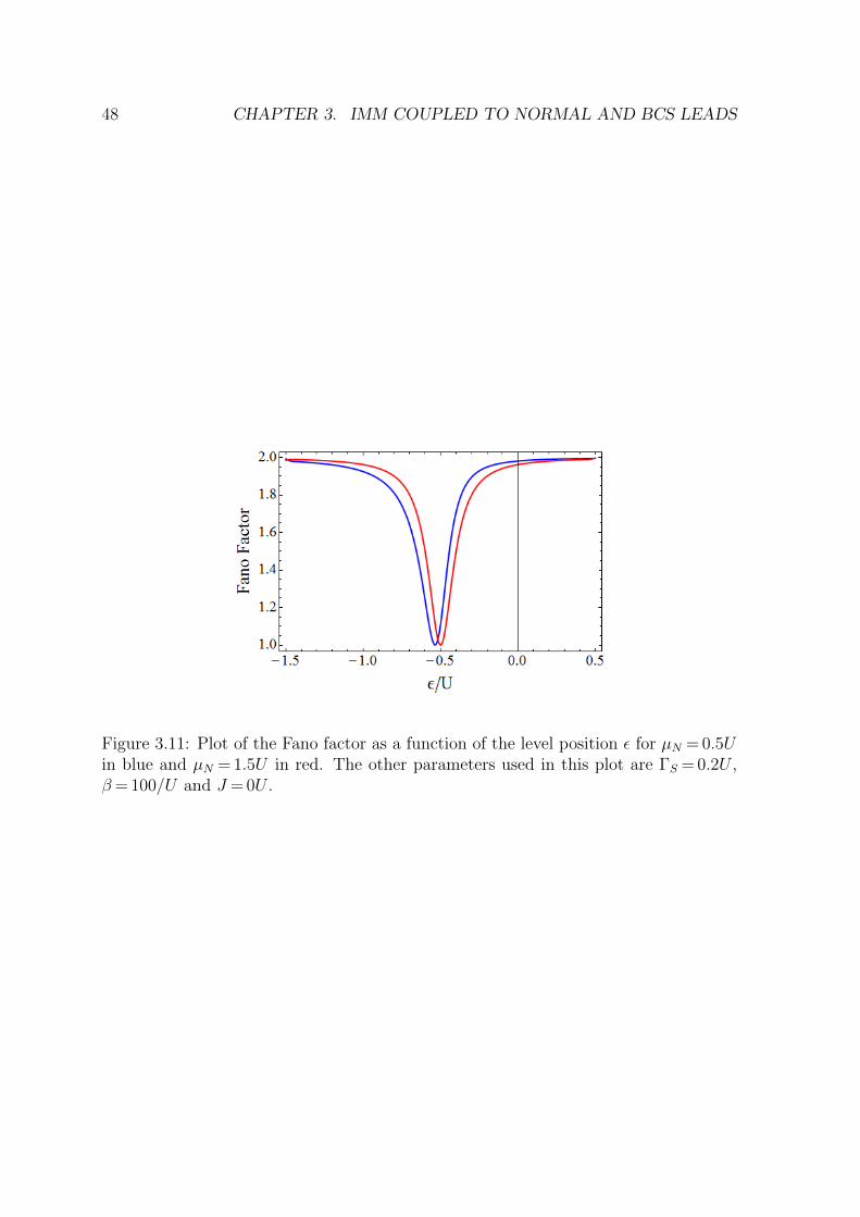
48 CHAPTER 3. IMM COUPLED TO NORMAL AND BCS LEADS
Figure 3.11: Plot of the Fano factor as a function of the level position ε for µN = 0.5Uin blue and µN = 1.5U in red. The other parameters used in this plot are ΓS = 0.2U ,β= 100/U and J = 0U .

Chapter 4
Anisotropic Magnetic Molecule
Coupled to Normal and BCS Leads
In the previous chapter we studied an isotropic magnetic molecule. However some
realistic magnetic molecules, such as Mn12 [25], are anisotropic, therefore in this chapter
we will analyse the current through an anisotropic magnetic molecule (AMM). All
calculations in this chapter will be performed in the same way as in the previous
chapter. In the anisotropic model we will include a quantum tunneling of magnetisation
term and an anisotropy term.
4.1 N-AMM-S System
Figure 4.1: A single level anisotropic magnetic molecule coupled to a superconductinglead and a normal lead, with coupling strengths ΓS and ΓN , and exchange coupling, J ,between the spin of the electrons occupying the orbital level and the spin of the restof the molecule.
To model an anisotropic magnetic molecule we add an anisotropy term, D, and
49

50 CHAPTER 4. AMM COUPLED TO NORMAL AND BCS LEADS
a quantum tunneling of magnetisation term, M , to the Hamiltonian of the magnetic
molecule to give
HM =∑σ
εd+σ dσ + Un↑n↓ −DS2
Z +M
2(S2
+ + S2−) + JS.se, (4.1)
where S+ and S− are the ladder operators for the molecular spin. All other terms have
the same definitions as in the previous chapter. The lead and tunneling Hamiltonians
are the same as in Chapter 3 (Eqs. 3.12 and 3.13). The QTM term couples states with
different molecular spins, as depicted in Fig. 4.2. We have only included the lowest order
QTM term as higher order terms (Mn
2
(S2n
+ + S2n−), n= 2, 3, ...) are usually small [21].
Figure 4.2: Quantum tunneling of magnetisation allows coupling between molecularspin states two levels apart. For S=1 QTM couples the |1〉M and | − 1〉M states.
The effect of the superconducting lead, to all orders in tunnel coupling, is again
taken into account by using an effective Hamiltonian to describe MM-S subsytem. This
effective Hamiltonian is now given by
Heff =∑σ
εd+σ dσ + Un↑n↓ −DS2
Z +M
2(S2
+ + S2−) + JS.se −
ΓS2
(d+↑ d
+↓ + d↓d↑). (4.2)
The coupling to the superconducting lead gives rise to the same term in the effective
Hamiltonian as in the previous chapter. This is because the superconducting proximity
effect only causes superpositions of |0〉e and |d〉e states that have the same molecular
spin.
For simplicity we will use the smallest molecular spin, S = 1, that will show the
effects of the anisotropy and QTM. With S=1 there are now twelve states in this
system; |0, 0〉, |d, 0〉, |0,−1〉, |d,−1〉, |0, 1〉, |d, 1〉, | ↑, 0〉, | ↓, 1〉, | ↓,−1〉, | ↓, 0〉, | ↑,−1〉,

4.1. N-AMM-S SYSTEM 51
| ↑, 1〉. The effective Hamiltonian is block diagonal and the sub-matrices are given by
HA =
(0 −ΓS
2−ΓS
22ε+ U
), (4.3)
HB =
−D −ΓS
2−M 0
−ΓS2
2ε+ U −D 0 −M−M 0 −D −ΓS
2
0 −M −ΓS2
2ε+ U −D
(4.4)
and
HC/D =
ε J√2
0J√2
ε−D − J2
−M0 −M ε−D + J
2
(4.5)
with the bases {|0, 0〉, |d, 0〉}, {|0,−1〉, |d,−1〉, |0, 1〉, |d, 1〉}, {| ↑, 0〉, | ↓, 1〉, | ↓,−1〉}and {| ↓, 0〉, | ↑,−1〉, | ↑, 1〉} for HA, HB, HC and HD, respectively. Diagonalising these
matrices leads to eigenstates of the form
|A〉 = X1A|0, 0〉+X2A|d, 0〉, (4.6)
|B〉 = X1B|0,−1〉+X2B|d,−1〉+X3B|0, 1〉+X4B|d, 1〉, (4.7)
|C〉 = X1C | ↑, 0〉+X2C | ↓, 1〉+X3C | ↓,−1〉 (4.8)
and
|D〉 = X1D| ↓, 0〉+X2D| ↑,−1〉+X3D| ↑, 1〉, (4.9)
where A→ A1, A2, B → B1, B2, B3, B4, C → C1, C2, C3 and D → D1, D2, D3. The
corresponding energies are given in Table 4.1 and the expressions for the eigenstate
coefficients can be found in the Appendix B.
The sub-matrix HA produces two Andreev bound states similar to those encoun-
tered in the previous model. If we were considering an isotropic molecule then there
would be four further Andreev bound states of the same form, two each for S= 1 and
S= -1. However due to the tunneling of magnetisation term in this model there is
coupling between states with S= 1 and S= -1. This leads to the form of the bound
states that arise from the diagonalisation of the matrix HB. The energies of these
states are very similar to the Andreev bound state energies of HA, however they have
an extra term for the anisotropy and the tunneling of magnetisation. The form of the
remaining six states arise due to the coupling of the electronic and molecular spins, as

52 CHAPTER 4. AMM COUPLED TO NORMAL AND BCS LEADS
χ A B C/D
Eχ1
δ2
+ εAδ2− εA −M −D Re
[γ+β2+i
√3(γ−β2)2
12β
]+ 3ε−2D
3
Eχ2
δ2− εA δ
2− εA +M −D Re
[γ+β2−i
√3(β2−γ)2
12β
]+ 3ε−2D
3
Eχ3 - δ2
+ εA −M −D Re[−γ+β2
6β
]+ 3ε−2D
3
Eχ4 - δ2
+ εA +M −D -
Table 4.1: Energies of the 12 eigenstates of the anisotropic system. δ and εA are definedas in Chapter 3. The other terms are defined as β= (
√α+ 72M2D − 8D3 + 27J3)1/3,
γ= 12M2 + 4D2 + 9J2 and α=−(12M2 + 4D2 + 9J2)3 + (72M2D − 8D3 + 27J3)2.
well as the tunneling of magnetisation. The X1χ|σ, 0〉+ X2χ|σ,±1〉 terms are similar
to the singlet and |T0〉 states of the previous model.
4.2 Transition Rates and Current
Because we are still only interested in transport to first order in ΓN , and there are no
off-diagonal reduced density matrix elements that contribute to the dynamics of the
system, we can once again use Fermi’s golden rule to calculate the transition rates. The
transitions that are made possible by first order tunneling events are |χ〉 |χ′〉, with
χ=A,B and χ′=C,D. Calculating the corresponding generalised transition rates we
get
WA,C/C,A = ΓN |X1C |2[|X1A|2f−/+ (EC − EA) + |X2A|2f+/− (EA − EC)
], (4.10)
WA,D/D,A = ΓN |X1D|2[|X1A|2f−/+ (ED − EA) + |X2A|2f+/− (EA − ED)
], (4.11)
WB,C/C,B = ΓN
[|X1BX3C +X3BX2C |2f−/+ (EC − EB)
+|X2BX3C +X4BX2C |2f+/− (EB − EC)]
(4.12)
and
WB,D/D,B = ΓN
[|X1BX2D +X3BX3D|2f−/+ (ED − EB)
+|X2BX2D +X4BX3D|2f+/− (EB − ED)]. (4.13)

4.3. RESULTS 53
Using these rates we calculate the current in the same way as in Chapter 3. For
this system we are not able to obtain analytic results. Therefore in the next section
we will analyse numerical results, as was done in Chapter 3.
4.3 Results
Figure 4.3: Density plots of the current (a) and the differential conductance (b) asfunctions of the chemical potential µN and the level position ε. The other parametersused in these plots are ΓS = 0.5U , kBT = 0.02U , J = 0.2U , D= 0.2U and M = 0.1U .
Figure 4.3 shows an example of the current and differential conductance of the
N-AMM-S system. These plots are very similar to those of the N-IMM-S system
analysed in Chapter 3, however we see more features due to the larger Hilbert space of
this system. In the limit of J tending to zero the dynamics of the anisotropic magnetic
molecule reduce to those of a single level quantum dot. The anisotropy and the QTM
have no affect in this limit as it is only through the exchange coupling between the
electronic and molecular spins that the molecular spin influences the dynamics of the
system. The effect that the strength of the exchange coupling has on the current is
the same as in the previous model. As J is increased the central low conduction region
becomes larger and some of the Andreev bound states start to overlap which causes
some features to disappear (Fig. 4.4).
At high bias, when all transitions are possible, the maximum current and the width
of the current resonance are unaffected by D or M . This is not immediately obvious
from the transition rates due to the intricate forms of the prefactors. To investigate

54 CHAPTER 4. AMM COUPLED TO NORMAL AND BCS LEADS
Figure 4.4: Plot of the current as a function of the chemical potential µN for J = 0.1,0.3 and 0.6U . The other parameters used in this plot are ΓS = 0.5U , ε= -0.5U ,kBT = 0.02U , D= 0.2U and M = 0.1U .
the effect of the D and M on the bias dependents of the current we have plotted the
current as a function of µN in Figs. 4.5 and 4.6. For these plots ε= -0.5U , meaning the
superconducting proximity effect is in resonance. Here we see that changing D or M
does not have a significant effect on the current, especially compared to the effect of
changing J (Fig. 4.4). For the anisotropy this could be because, apart from the |A〉states, all states are affected by the anisotropy to a similar degree and therefore the
anisotropy mostly cancels out in the excitation energies.
As the changes in the current are relatively small as D and M are varied, we have
plotted the differential conductance in Figs. 4.7 and 4.8, again for the superconducting
proximity effect in resonance. In Fig. 4.7 the QTM is zero and the plots are made for
various magnitudes of the anisotropy. In Fig. 4.8 the anistropy is zero and the plots are
made for various QTM values. Here we see that for the smaller D and M values there
are more differential conductance peaks. As |µN | is increased from zero the first peak
is largest for greater D and M values. This is because when D and M are sufficiently
large some of the excitation energies cross, meaning that when µN is high enough for
the system to tunnel out of the ground state several transport channels are opened at
once causing a greater increase in the current than for smaller D and M , where the
additional channels are opened at slightly higher |µN | values. For this system we have
not plotted the excitation energies as there are too many for a visual representation to
be meaningful, however the effect is the same described in reference to Fig. 3.10 in the
previous chapter. In Figs. 4.9 and 4.10 we have plotted the differential conductance

4.4. N-AMM-S CONCLUSIONS 55
Figure 4.5: Plot of the current as a function of the chemical potential µN for D= 0.1,0.3 and 0.6U . The other parameters used in this plot are ΓS = 0.5U , ε= -0.5U ,kBT = 0.02U , J = 0.2U and M = 0.1U .
for ε= -1.1U . In these plots there is a negative differential conductance feature for
D= 0.1U and M = 0.1U , respectively. The feature for D= 0.1U is however very small.
The expectation values of the electronic and molecular spins are zero for all param-
eter values. This can be deduced from the eigenstates. The electron spin expectation
value is zero because the kets with opposite electron spins, in the |C〉 and |D〉 eigen-
states, have the same prefactors and therefore contribute equally to the spin expectation
value. For the same reasons the |C〉 and |D〉 states do not contribute to the expectation
value of the molecular spin. The |B〉 states also do not give rise to non-zero molecular
spin expectation values because for these states the magnitude of the prefactors of the
kets with opposite molecular spins are the same.
4.4 N-AMM-S Conclusions
In this chapter we modified the model of Chapter 3 to allow for the molecule to be
anisotropic. To see the affects of the anisotropy and QTM we chose the spin of the
molecule to be S= 1. The results for the current were similar to those found in the
previous chapter. As a function of the applied bias and the level position, the current
and differential conductance map out the excitation energies, meaning that current
measurements should provide information on the anisotropy of a molecule. We found
that the anisotropy and the QTM do not affect the maximum current or the resonance
conditions of the proximity effect when the bias is greater than all excitation energies.

56 CHAPTER 4. AMM COUPLED TO NORMAL AND BCS LEADS
Figure 4.6: Plot of the current as a function of the chemical potential µN for M = 0.1,0.3 and 0.6U . The other parameters used in this plot are ΓS = 0.5U , ε= -0.5U ,kBT = 0.02U , J = 0.2U and D= 0.2U .
Although changes in the differential conductance can be observed as D and M are
varied, these parameters have little effect on the current compared with the effect of
the exchange coupling. Certain D or M values can however cause negative differential
conductances. For this system we also find that the spin expectation values are zero,
meaning that neither the spin of the electron or the molecule can be tuned using the
bias voltage or by applying a gate voltage.

4.4. N-AMM-S CONCLUSIONS 57
Figure 4.7: Plot of the differential conductance as a function of the chemical potentialµN for D= 0.1, 0.3 and 0.6U . The other parameters used in this plot are ΓS = 0.5U ,ε= -0.5U , kBT = 0.02U , J = 0.2U and M = 0.1U .
Figure 4.8: Plot of the differential conductance as a function of the chemical potentialµN for M = 0.1, 0.3 and 0.6U . The other parameters used in this plot are ΓS = 0.5U ,ε= -0.5U , kBT = 0.02U , J = 0.2U and D= 0.2U .

58 CHAPTER 4. AMM COUPLED TO NORMAL AND BCS LEADS
Figure 4.9: Plot of the differential conductance as a function of the chemical potentialµN for D= 0.1, 0.3 and 0.6U . For D= 0.1U there is negative differential conductancefeature near µN = 0.2U . The other parameters used in this plot are ΓS = 0.5U , ε= -1.1U , kBT = 0.02U , J = 0.2U and M = 0.1U .
Figure 4.10: Plot of the differential conductance as a function of the chemical potentialµN for M = 0.1, 0.3 and 0.6U . For M = 0.1U there is negative differential conductancefeature near µN = 0.1U . The other parameters used in this plot are ΓS = 0.5U , ε= -1.1U , kBT = 0.02U , J = 0.2U and D= 0.2U .

Chapter 5
Josephson Current
In the previous two chapters we have analysed the current through an isotropic and
an anisotropic magnetic molecule coulped to normal and superconducting leads. In
this chapter will replace the normal lead with a second superconducting lead to derive
the Josephson current through the two magnetic molecules. Such systems have been
analysed in recent years [20,21], however in these studies the superconducting gap was
finite and the charging energy U was infinite, and the current was only calculated to
second order in tunnel coupling. In these limits the electrons of a Cooper pair can-
not tunnel simultaneously to and from the superconducting leads. Instead, transport
between the molecule and the leads involves the transfer of quasi-particles. We will
once again work in the finite U and ∆→∞ limits and we will calculate the Josephson
current to all orders in the coupling to the superconducting leads. In references [20]
and [21] it is found that for strong anti-ferromagnetic coupling between the electronic
and molecular spins a 0-π transition is induced. For this transition to occur the sign
of the current must change. This can be achieved if the order in which the electrons
of a Cooper pair are created on the molecule is switched. However in the ∆ → ∞limit the electrons of a Cooper pair tunnel simultaneously, therefore no 0-π transition
is excepted in this case.
5.1 S-MM-S Systems
To describe the molecules we use Eqs. 3.2 and 4.1. The superconducting leads and
tunneling coupling are described by
Hη =∑k,σ
εkC+ηkσCηkσ −∆
∑k
(Cη−k↓Cηk↑ +H.c.) (5.1)
59

60 CHAPTER 5. JOSEPHSON CURRENT
Figure 5.1: Single level magnetic molecule tunnel coupled to two superconductingleads, with coupling strengths ΓL, ΓR and exchange coupling, J , between the spin ofthe electrons occupying the orbital level and the spin of the rest of the molecule.
and
Htunn,η =∑k,σ
(VηC+ηkσdσ +H.c.), (5.2)
where η=L,R for the left and right superconducting leads. All other symbols have the
same meaning as in Chapter 3.
We will calculate the Josephson current to all orders in tunnel coupling to the
superconducting leads. In order to do this we once again use an effective Hamiltonian
to describe the effect of coupling to these leads. For the case of a single level Anderson
model dot between two superconducting leads the effective Hamiltonian was derived by
Rozhkov and Arovas [50]. This Hamiltonian can easily be modified for the isotropic and
anisotropic magnetic molecule cases by adding the exchange coupling, the anisotropy
and the quantum tunneling of magnetisation terms. The effective Hamiltonians for the
isotropic and anisotropic molecules are
HIeff =∑σ
εd+σ dσ + Un↑n↓ + JS.se −
χS2d+↑ d
+↓ −
χ∗S2d↓d↑ (5.3)
and
HAeff =∑σ
εd+σ dσ +Un↑n↓−DS2
Z +B2
2(S2
+ +S2−) +JS.se−
χS2d+↑ d
+↓ −
χ∗S2d↓d↑, (5.4)
respectively. Here χS = ΓLeiφL+ΓRe
iφR , where Γη and φη are the coupling strength and
the phase of superconducting lead η. We once again choose S= 1/2 for the isotropic
case and S=1 for the anisotropic case.
The eigenstates of the effective Hamiltonians that involve single occupation of the
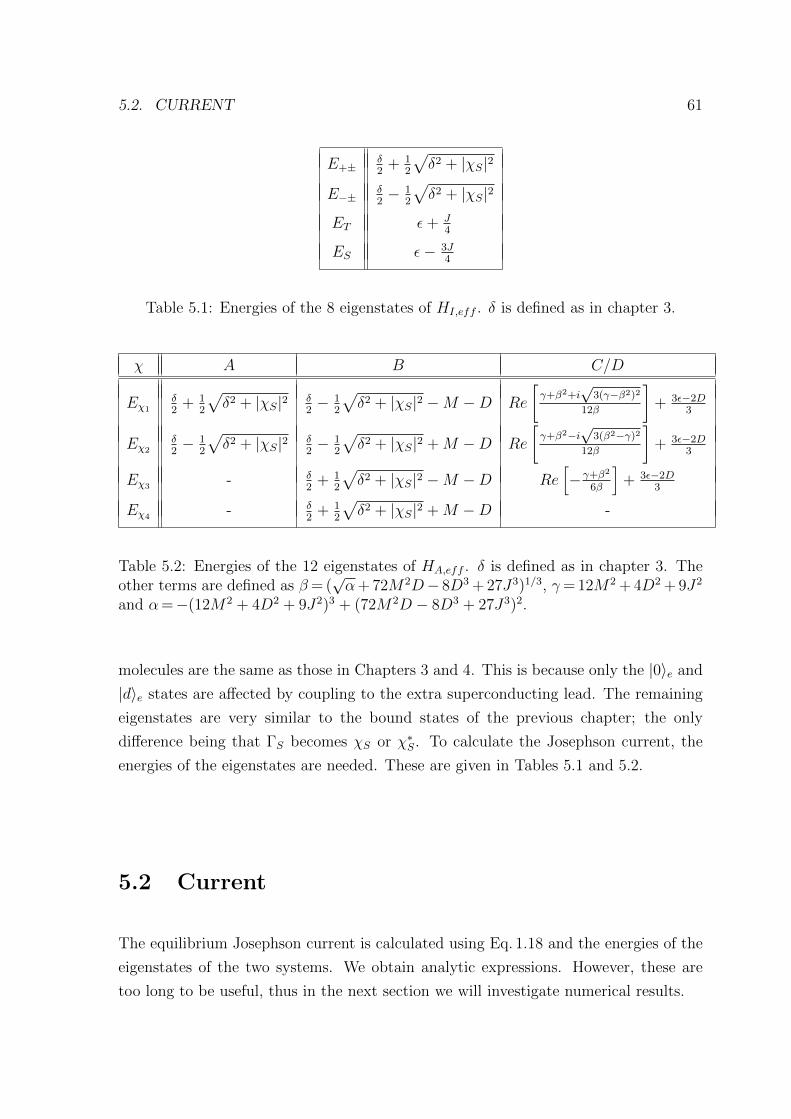
5.2. CURRENT 61
E+±δ2
+ 12
√δ2 + |χS|2
E−±δ2− 1
2
√δ2 + |χS|2
ET ε+ J4
ES ε− 3J4
Table 5.1: Energies of the 8 eigenstates of HI,eff . δ is defined as in chapter 3.
χ A B C/D
Eχ1
δ2
+ 12
√δ2 + |χS|2 δ
2− 1
2
√δ2 + |χS|2 −M −D Re
[γ+β2+i
√3(γ−β2)2
12β
]+ 3ε−2D
3
Eχ2
δ2− 1
2
√δ2 + |χS|2 δ
2− 1
2
√δ2 + |χS|2 +M −D Re
[γ+β2−i
√3(β2−γ)2
12β
]+ 3ε−2D
3
Eχ3 - δ2
+ 12
√δ2 + |χS|2 −M −D Re
[−γ+β2
6β
]+ 3ε−2D
3
Eχ4 - δ2
+ 12
√δ2 + |χS|2 +M −D -
Table 5.2: Energies of the 12 eigenstates of HA,eff . δ is defined as in chapter 3. Theother terms are defined as β= (
√α+ 72M2D− 8D3 + 27J3)1/3, γ= 12M2 + 4D2 + 9J2
and α=−(12M2 + 4D2 + 9J2)3 + (72M2D − 8D3 + 27J3)2.
molecules are the same as those in Chapters 3 and 4. This is because only the |0〉e and
|d〉e states are affected by coupling to the extra superconducting lead. The remaining
eigenstates are very similar to the bound states of the previous chapter; the only
difference being that ΓS becomes χS or χ∗S. To calculate the Josephson current, the
energies of the eigenstates are needed. These are given in Tables 5.1 and 5.2.
5.2 Current
The equilibrium Josephson current is calculated using Eq. 1.18 and the energies of the
eigenstates of the two systems. We obtain analytic expressions. However, these are
too long to be useful, thus in the next section we will investigate numerical results.

62 CHAPTER 5. JOSEPHSON CURRENT
5.3 Results
In the J →0 limit the there is no coupling between the electronic and molecular spins
and the singly occupied states of the isotropic molecule become degenerate. In this
limit the result for the Josephson current reduces to that for a single level quantum
dot in place of the molecule. Governale et al. have calculated the Josephson current
for the S-QD-S system, in the ∆ → ∞ limit, to second order in the coupling to the
leads. Setting J = 0, ΓL = ΓR≡ΓS and taking the terms up to second order in the
Taylor expansion of the current through the isotropic molecule, we find
Ijos =
(eU+2εkBT − 1
)Γ2Ssinφ(
1 + 2eU+εkBT + e
U+2εkBT
)(U + 2ε)
, (5.5)
which is in agreement with the result of Governale et al. [5].
Figure 5.2: Density plots of the Josephson current through (a) the isotropic and (b)the anisotropic magnetic molecules as functions of the exchange coupling U and thelevel position ε. The other parameters used in these plots are φ=π/2, kBT = 0.5ΓS,J = 0.2ΓS, D= 0.3ΓS and M = 0.2ΓS.
Figures 5.2 a) and b) show density plots of the Josephson current for the isotropic
and anisotropic molecules, respectively. Here and in all subsequent plots we have chosen
ΓL = ΓR≡ΓS. In plot b) there is no noticeable difference due to the anisotropy or the
QTM compared with the isotropic molecule. Both plots show that as U increases the
current tends to zero in the negative ε half plane. In the positive ε half plane the
ground states of the isotropic system are the | − ±〉 states and these states contribute

5.3. RESULTS 63
to the Josephson current. But for large U > ε in the negative ε half plane the ground
state is |S〉, which does not contribute to the Josephson current, as this state does not
couple to the superconducting leads. This occurs similarly for states of the anisotropic
molecule. The current is greatest when U = ε= 0, because there the energy of the
lowest bound state is minimised.
In Fig. 5.2 we see that the anisotropy and QTM of the anisotropic molecule do not
have a significant effect on the current. To quantify the influence of these parameters
we have plotted the current as functions of D and M in Figs. 5.3 and 5.4. In both
cases the current increases with the magnitude of the parameter, but only by a few
percent. This is probably because D and M affect all of the lowest energy eigenstates
in a similar manner.
Figure 5.3: Plot of the current through the anisotropic molecule as a function of D atδ= 0. The other parameters used in this plot are φ=π/2, kBT = 0.5ΓS, J = 0.2ΓS andM = 0.2ΓS.
To analyse the affect of the exchange coupling we will concentrate on the isotropic
molecule. Figure 5.5 a) and b) show density plots of the Josephson current for J = 3ΓS
and J =−3ΓS. Compared with Fig. 5.2 a) the current is decreased for both plots. For
large positive J values the parameter range over which the singlet state is the ground
state increases. This is shown by the larger zero current region. When J is negative the
triplet states are lower in energy than the singlet and are therefore the ground states
in the zero current region.
Shown in Fig. 5.6 are density plots of the Josephson current through the isotropic
molecule at kBT = 0.1ΓS and kBT = 1.0ΓS. Note that the scales for these plots are

64 CHAPTER 5. JOSEPHSON CURRENT
Figure 5.4: Plot of the current through the anisotropic molecule as a function of M atδ= 0. The other parameters used in this plot are φ=π/2, kBT = 0.5ΓS, J = 0.2ΓS andD= 0.2ΓS.
different. As expected, the transition form the zero current region to the non-zero cur-
rent region becomes sharper as the temperature is lowered. In Fig. 5.2 a) kBT = 0.5ΓS.
Comparing this plot with Fig. 5.6 b) we see that with U and ε scaled by the same factor
as the temperature the current features appear the same, but the magnitude is approx-
imately halved for the factor of two increase in the temperature. This trend occurs
because as the temperature increases the eigenstates contribution more equally to the
partition function, meaning that the denominator of Eq. 1.18 increases with respect to
the numerator. We also see that in Fig. 5.6 a) the current is larger than for the higher
temperature plots.
The phase dependence of the Josephson current is approximately sinusoidal. To
second order the Josephson current through a quantum dot depends on sinφ (Eq. 5.5),
but because we have calculated the current to all orders in ΓS for the magnetic molecule
systems, this is not exactly correct. However deviations from the sine dependence are
not noticeable in the numerical results. We also find that for both the isotropic and
the anisotropic cases there is no 0-π phase transition. As the parameters are varied
the current can tend to zero, however it never changes sign. This is as expected since
no quasi-particle states are allowed in the leads.

5.4. JOSEPHSON CURRENT CONCLUSIONS 65
Figure 5.5: Density plots of the Josephson current through the isotropic magneticmolecule as a function of the exchange coupling U and the level position ε for (a)J = 3ΓS and (b) J = -3ΓS. The other parameters used in these plots are φ=π/2 andkBT = 0.5ΓS.
5.4 Josephson Current Conclusions
In this chapter we calculated the equilibrium Josephson current through an isotropic
and an anisotropic magnetic molecule coupled to two infinite gap superconducting
leads. We found that no 0-π transition is induced for any parameter values and that the
anisotropy and QTM have negligible affect on the current. Strong exchange coupling
between the electronic and molecular spins decreases the current, as it lowers the energy
of at least one of the singly occupied states and these do not contribute to the current.

66 CHAPTER 5. JOSEPHSON CURRENT
Figure 5.6: Density plots of the Josephson current through the isotropic as a func-tion of the exchange coupling U and the level position ε for (a) kBT = 0.1ΓS and (b)kBT = 1.0ΓS. The other parameters used in these plots are φ=π/2 and J = 0.2ΓS.

Chapter 6
Isotropic Magnetic Molecule
Coupled to Ferromagnetic and BCS
Leads
In Chapter 3 we studied an isotropic magnetic molecule between a superconducting
lead and a normal metallic lead. In this chapter we will modify this system to allow
for the normal lead to be ferromagnetic and for the presence of an external magnetic
field. The motivation for this is that it will add spin dependence to the current. In
Chapter 3 we found that even though the molecule is magnetic the spin expectation
values were zero, meaning that the current has no overall spin dependence. However
with the normal lead now ferromagnetic more of the majority spins will tunnel to and
from the molecule. This will change the non-equilibrium occupation probabilities of
the eigenstates of the IMM-S subsystem and cause non-zero spin expectation values.
For simplicity we will only consider the isotropic molecule in this chapter, as this shows
interesting properties without having to work in the larger Hilbert space that is required
for the anisotropic molecule.
We will allow for arbitrary alignment of the magnetisation of the ferromagnetic
lead and the external magnetic field. This will lead to off-diagonal reduced density
matrix elements contributing to the dynamics of the system. To calculate generalised
transition rates involving these off-diagonal elements we will use the diagrammatic
technique described in Chapter 2, since to the best our knowledge this is not possible
using Fermi’s golden rule.
67
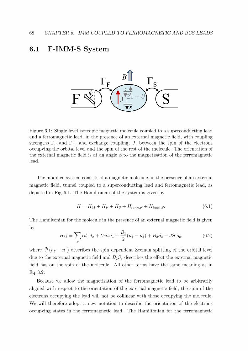
68 CHAPTER 6. IMM COUPLED TO FERROMAGNETIC AND BCS LEADS
6.1 F-IMM-S System
Figure 6.1: Single level isotropic magnetic molecule coupled to a superconducting leadand a ferromagnetic lead, in the presence of an external magnetic field, with couplingstrengths ΓS and ΓF , and exchange coupling, J , between the spin of the electronsoccupying the orbital level and the spin of the rest of the molecule. The orientation ofthe external magnetic field is at an angle φ to the magnetisation of the ferromagneticlead.
The modified system consists of a magnetic molecule, in the presence of an external
magnetic field, tunnel coupled to a superconducting lead and ferromagnetic lead, as
depicted in Fig. 6.1. The Hamiltonian of the system is given by
H = HM +HF +HS +Htunn,F +Htunn,S. (6.1)
The Hamiltonian for the molecule in the presence of an external magnetic field is given
by
HM =∑σ
εd+σ dσ + Un↑n↓ +
B1
2(n↑ − n↓) +B2Sz + JS.se, (6.2)
where B1
2(n↑ − n↓) describes the spin dependent Zeeman splitting of the orbital level
due to the external magnetic field and B2Sz describes the effect the external magnetic
field has on the spin of the molecule. All other terms have the same meaning as in
Eq. 3.2.
Because we allow the magnetisation of the ferromagnetic lead to be arbitrarily
aligned with respect to the orientation of the external magnetic field, the spin of the
electrons occupying the lead will not be collinear with those occupying the molecule.
We will therefore adopt a new notation to describe the orientation of the electrons
occupying states in the ferromagnetic lead. The Hamiltonian for the ferromagnetic

6.1. F-IMM-S SYSTEM 69
lead is now given by
HF =∑k,α
εkC+F,k,αCF,k,α, (6.3)
where α = +,− stands for the majority and minority spins, respectively. The majority
spins point in the direction of the magnetisation of the lead, whereas the minority
spins point in the opposite direction. The Hamiltonian describing tunneling between
the molecule and the ferromagnetic lead is given by
Htunn,F =∑k,σ,α
(VF,σ,αC+F,k,αdσ +H.c.). (6.4)
The matrix elements VF,σ,α are no longer diagonal in spin space due to the different
quantisation axes of the lead and IMM-S subsystem. The individual tunneling ampli-
tudes are given by VFUσα, where Uσα is a SU(2) rotation matrix, the form of which
depends on the geometry of the system, and VF is the tunneling amplitude, which is
assumed to be independent of spin and energy. We will consider the spin-quantisation
axes of the lead and the IMM-S subsystem in the x-z plane and use the matrix for
rotations about the y-axis, Uy(φ). The tunneling Hamiltonian then becomes
Htunn,F =∑
k VF
(cos(φ2
)C+Fk+d↑ − sin
(φ2
)C+Fk+d↓
+sin(φ2
)C+Fk−d↑ + cos
(φ2
)C+Fk−d↓ +H.c.
), (6.5)
where φ is the angle between the quantisation axes of the magnetisation of the ferro-
magnetic lead and the external magnetic field, as shown in Fig. 6.1. The maximum
tunnel couplings for the majority and minority spins are given by ΓF± = 2πρ±|VF |2,
where ρ± are the energy independent density of states for the majority and minority
spins in the ferromagnetic lead. It is useful to express these tunnel coupling strengths
in terms of ΓF = ΓF++ΓF−2
and to use the polarisation P = ρ+−ρ−ρ++ρ−
.
The Hamiltonians describing the superconducting lead and tunneling to and from
the superconducting are still given by Eqs. 3.12 and 3.13 in Chapter 3, and once again
we take into account the effect of the superconducting lead by introducing an effective
Hamiltonian,
Heff = HM −ΓS2
(d+↑ d
+↓ + d↓d↑). (6.6)
For simplicity we again choose the molecular spin to be S=1/2. Using the basis
{|0, 1/2〉, |d, 1/2〉, |0,−1/2〉, |d,−1/2〉, | ↑, 1/2〉, | ↓,−1/2〉, | ↓, 1/2〉, | ↑,−1/2〉}, we can
write the effective Hamiltonian in matrix form. This matrix is block diagonal and can

70 CHAPTER 6. IMM COUPLED TO FERROMAGNETIC AND BCS LEADS
therefore be broken into two blocks, the first involving the empty and doubly occupied
states and the second involving the singly occupied states:
Heff1 =
B2
2−ΓS
20 0
−ΓS2
2ε+ U + B2
20 0
0 0 −B2
2−ΓS
2
0 0 −ΓS2
2ε+ U − B2
2
, (6.7)
Heff2 =
ε+ J
4+ B1+B2
20 0 0
0 ε+ J4− B1+B2
20 0
0 0 ε− J4− B1−B2
2J2
0 0 J2
ε− J4
+ B1−B2
2
. (6.8)
We diagonalise these matrices to find the energies and eigenstates of this system for
zero coupling to the ferromagnetic lead. Compared with the eigenstates of the system
studied in Chapter 3 the degeneracy of the Andreev bound state pairs has been lifted
due to the magnetic field acting on the molecular spin. The four bound states and
their respective energies are now given by
|+,±〉 =1√2
√1− δ
2εA|0,±1/2〉 − 1√
2
√1 +
δ
2εA|d,±1/2〉 (6.9)
E+± =δ
2+ εA ±
B2
2(6.10)
and
|−,±〉 =1√2
√1 +
δ
2εA|0,±1/2〉+
1√2
√1− δ
2εA|d,±1/2〉 (6.11)
E−± =δ
2− εA ±
B2
2. (6.12)
The definitions of δ and εA are those given in Chapter 3.
In Chapter 3 the remaining four states formed a singlet and a triplet. The states
in this system still resemble those of Chapter 3 but the degeneracy of the triplet states
has been lifted. The states and their energies are now given by
|I+〉 = | ↑, 1/2〉 (6.13)
EI+ = ε+J
4+B1 +B2
2, (6.14)

6.2. TRANSITION RATES AND CURRENT 71
|I−〉 = | ↓,−1/2〉 (6.15)
EI− = ε+J
4− B1 +B2
2, (6.16)
|I0〉 =λ1+√
2| ↓, 1/2〉+
λ2+√2| ↑,−1/2〉 (6.17)
EI0 = ε− J
4+
1
2
√(B1 −B2)2 + J2 (6.18)
and
|IS〉 =λ1−√
2| ↓, 1/2〉 − λ2−√
2| ↑,−1/2〉 (6.19)
EIS = ε− J
4− 1
2
√(B1 −B2)2 + J2. (6.20)
The prefactors of the kets in the states |IS〉 and |I0〉 are
λ1± =
√J2
J2 + (B1 −B2)2 ± (B1 −B2)√
(B1 −B2)2 + J2(6.21)
and
λ2± =
√J2 + 2(B1 −B2)2 ± 2(B1 −B2)
√(B1 −B2)2 + J2
J2 + (B1 −B2)2 ± (B1 −B2)√
(B1 −B2)2 + J2. (6.22)
In the limit B1 =B2 →0 the eigenstates reduce to the Andreev bound states and
triplet-singlet of Chapter 3. We will label the excitation energies as |Eab|=±|Ea−Eb|.
6.2 Transition Rates and Current
When φ 6= 0 the spin of the electron is not conserved in individual tunneling events
between the molecule and the ferromagnetic lead. Due to this there are off-diagonal
reduced density matrix elements that can contribute to the dynamics of the system.
However, when φ= 0 no off-diagonal elements should be included. We will therefore
treat the two cases separately. First we will calculate the rates for the collinear case,
φ= 0, then we will consider the non-collinear case, φ 6= 0.

72 CHAPTER 6. IMM COUPLED TO FERROMAGNETIC AND BCS LEADS
6.2.1 Collinear
As the electronic and molecular spins are conserved during tunneling events the gener-
alised transition rates contributing to the dynamics of the system are still restricted to
those given in Chapter 3. We do not have to consider any off-diagonal reduced density
matrix elements and therefore can once again use Fermi’s golden rule to calculated the
first order rates. Because in this case the spin of the electrons in the ferromagnetic
lead are aligned with those on the molecule it is more convenient to let α= ↑, ↓ instead
of +,−. Therefore we define the polarisation and average coupling strength as
P =ρ↑ − ρ↓ρ↑ + ρ↓
(6.23)
and
ΓF =ΓF↑ + ΓF↓
2, (6.24)
respectively. It is convenient to write ΓF↑ and ΓF↓ in terms of P and ΓF , giving
ΓF↑ = (1 + P )ΓF (6.25)
and
ΓF↓ = (1− P )ΓF . (6.26)
The non-zero transition rates are
W±+I+ =ΓF2
[(1− P ) δ2
±f+ (E±+ − EI+) + (1 + P ) δ2
∓f− (EI+ − E±+)
], (6.27)
WI+±+ =ΓF2
[(1− P ) δ2
±f− (E±+ − EI+) + (1 + P ) δ2
∓f+ (EI+ − E±+)
], (6.28)
W±−I− =ΓF2
[(1 + P ) δ2
±f+ (E±− − EI−) + (1− P ) δ2
∓f− (EI− − E±−)
], (6.29)
WI−±− =ΓF2
[(1 + P ) δ2
±f− (E±− − EI−) + (1− P ) δ2
∓f+ (EI− − E±−)
], (6.30)
W±+η =ΓFλ
21ζ
4
[(1 + P ) δ2
±f+ (E±+ − Eη) + (1− P ) δ2
∓f− (Eη − E±+)
], (6.31)
Wη±+ =ΓFλ
21ζ
4
[(1 + P ) δ2
±f− (E±+ − Eη) + (1− P ) δ2
∓f+ (Eη − E±+)
], (6.32)
W±−η =ΓFλ
22ζ
4
[(1− P ) δ2
±f+ (E±− − Eη) + (1 + P ) δ2
∓f− (Eη − E±−)
](6.33)

6.2. TRANSITION RATES AND CURRENT 73
and
Wη±− =ΓFλ
22ζ
4
[(1− P ) δ±
2f− (E±− − Eη) + (1 + P ) δ2∓f
+ (Eη − E±−)]. (6.34)
Here η= I0, IS and ζ = + if η= I0 or ζ = - if η= IS. As in Chapter 3 δ2±=
(1± δ
2εA
).
The occupation probabilities, current and Fano factor are calculated using the same
methods as in Chapter 3.
6.2.2 Non-collinear
With eight eigenstates and without the requirement that the electronic spin be con-
served during tunneling events there are now off-diagonal reduced density matrix ele-
ments that effect the dynamics of the system. In the most general case there are over
200 generalised transition rates that are non-zero. Table 6.1 summarises the coher-
ent superpositions that must be taken into account for various parameter values. For
simplicity we have set B1 =B2 =B. To make the system of equations more manage-
able we will consider only case (iv)-b. The condition |2εA − B|.ΓN is satisfied when
2εA−B= 0. This can be rewritten to give the condition δ=±√B2 − Γ2
S. In this regime
there are only two off-diagonal reduced density matrix elements that contribute to the
current. The reduced density matrix of the molecule coupled to the superconducting
lead, in this regime, is
ρRM =
P++ 0 0 0 P++T1 0 0 0
0 P+− P+−−+ 0 0 0 P+−
T0 P+−S
0 P−++− P−+ 0 0 0 P−+
T0 P−+S
0 0 0 P−− 0 P−−T -1 0 0
P T1++ 0 0 0 PT1 0 0 0
0 0 0 P T -1−− 0 PT -1 0 0
0 P T0+− P T0
−+ 0 0 0 PT0 0
0 P S+− P S
−+ 0 0 0 0 PS
. (6.35)
The entries in red are non-zero but in first order they cannot couple to the diagonal
elements and therefore do not contribute to the dynamics of the system. With the ten
reduced density matrix elements that contribute to the dynamics of the system there
are 42 non-zero generalised transition rates that must be calculated.
As there are now non-zero off-diagonal reduced density matrix elements that con-
tribute to the dynamics of the system we can no longer use Fermi’s golden rule to

74 CHAPTER 6. IMM COUPLED TO FERROMAGNETIC AND BCS LEADS
Case Parameters Superpositions
(i) B . ΓN , J � ΓN |I+〉, |I−〉, |I0〉| ± ±〉, | ± ∓〉
(ii) B, J . ΓN |I+〉, |I−〉, |I0〉|I±〉, |IS〉|I0〉, |IS〉| ± ±〉, | ± ∓〉
(iii) J . ΓN , B � ΓN |I0〉, |IS〉a (if |2εA −B| . ΓN) (|+−〉, | −+〉)
(iv) B, J � ΓN none
a (if |J −B| . ΓN) (|I−〉, |IS〉)b (if |2εA −B| . ΓN) (|+−〉, | −+〉)
Table 6.1: Coherent superpositions of that have to be taken into account for variousparameter values are given in this table.
calculate all of the rates. Therefore we will use the diagrammatic technique outlined
in Chapter 2. Each generalised transition rate, Wχ2χ′2χ1χ′1
, can be represented by diagrams
such as that shown in Fig. 6.2. Then a set of rules can be used to write out the equa-
tions represented by these diagrams. To calculate the generalised transition rates of
this system, to first order in tunnel coupling ΓF , the diagrammatic rules are:
1. Draw all topologically different diagrams and assign energies to all propagators
and tunneling lines.
2. For each part of the diagram between adjacent vertices assign a resolvent 1∆E+i0+
,
where ∆E is the energy difference between left going and right going propagators
and tunneling lines.
3. For each tunneling line the diagram acquires a factor of f±(ω), - (+) for lines
running forward (backward) with respect to the Keldysh contour.
4. For each pair of vertices connected by a tunneling line the diagram is multiplied
by
ρ+〈χ′i|C+σ|χi〉〈χ′f |C++σ|χf〉+ ρ−〈χ′i|C−σ|χi〉〈χ′f |C+
−σ|χf〉 (6.36)
where χi and χ′i (χf and χ′f ) are the states that enter and leave the vertex
where the tunneling line begins (ends), respectively. The operators C(+)ασ are the

6.2. TRANSITION RATES AND CURRENT 75
coefficients (including the dot operators) of C(+)Fkα in the tunneling Hamiltonian.
5. The diagram is multiplied by a factor of −i(−1)a, where a is the number of
vertices on the lower propagator.
6. Integrate the diagram over all energies ω.
7. When calculating the generalised current rates multiply each diagram by 1 if the
line is going form the lower to the upper propagator and -1 if it is going from the
upper to the lower propagator, otherwise multiply the diagram by zero.
Figure 6.2: One of the possible transitions from P χ2χ1
to Pχ′2χ′1
. The top line represents
forward propagation in time and the bottom line backward propagation. The line withthe arrow head is the tunneling line and represents the contraction of two tunnelingvertices. The tunneling line points to where an electron is created on the orbitallevel of the molecule. The spin of the electrons destroyed and created on the dot arerepresented by σ and σ; these can be the same or different.
Figure 6.3 shows the diagrammatic representation of W+−+−−+−+ . Applying the di-
agrammatic rules to Fig. 6.3, and rewriting the equation in terms of ΓF and P , we
obtain
W+−+−−+−+ = −i
4π{ΓF (1 + P cosφ)(δ2
+
[∫ f−(ω)dωE−+−EI−−ω+i0+
+∫ f+(ω)dω
EI+−E+−−ω+i0+
]+
δ2−2
[∫ f+(ω)dωE−+−EI0+ω+i0+
+∫ f+(ω)dω
E−+−EIS+ω+i0++∫ f−(ω)dω
EI0−E+−+ω+i0++∫ f−(ω)dω
EIS−E+−+ω+i0+
])
+ΓF (1− P cosφ)(δ2−
[∫ f+(ω)dωE−+−EI−+ω+i0+
+∫ f−(ω)dω
EI+−E+−+ω+i0+
]+ (6.37)
δ2+2
[∫ f−(ω)dωE−+−EI0−ω+i0+
+∫ f−(ω)dω
E−+−EIS−ω+i0++∫ f+(ω)dω
EI0−E+−−ω+i0++∫ f+(ω)dω
EIS−E+−−ω+i0+
])}.
These integrals are then calculated using the residue theorem, which is given in Ap-
pendix C along with an example calculation. The expression for W+−+−−+−+ is rather

76 CHAPTER 6. IMM COUPLED TO FERROMAGNETIC AND BCS LEADS
Figure 6.3: All of the first order contributions to the generalised transition rate W+−+−−+−+ .
cumbersome and is therefore given in Appendix C, with all other non-zero generalised
transition rates. Here we give two example rates;
WI+±+ =ΓF2
[δ2± (1− P cosφ) f− (E±+ − EI+) + δ2
∓ (1 + P cosφ) f+ (EI+ − E±+)]
(6.38)
and
W±∓η∓±η = α iδ+δ−
8πΓFP sinφ
(iπ(f+ (E+− − Eη) + f+ (E−+ − Eη) + f− (Eη − E−+) +
f− (Eη − E+−) )∓ Re[Ψ(
12
+ iβ2π
(Eη − E+− − µF ))−Ψ
(12
+ iβ2π
(Eη − E−+ − µF ))]
∓Re[Ψ(
12
+ iβ2π
(E+− − Eη − µF ))−Ψ
(12
+ iβ2π
(E−+ − Eη − µF ))] )
. (6.39)
Ψ(x) is the digamma function, η= I0,IS and α= + (-) if η= I0 (IS).
To calculate the current we modify the generalised transition rates to obtain the

6.3. RESULTS - COLLINEAR 77
current rates. This is done by applying rule 7, given in the list of diagrammatic rule
presented in this section. These current rates are then used in Eq. 2.24. For the non-
collinear case we will not calculate the Fano factor as the method described in Chapter
2 is only valid for systems where no off-diagonal density matrix elements contribute to
the current.
6.3 Results - Collinear
In this section we will investigate the results of the collinear case. As in Chapter 3
it was not possible to obtain analytic expressions for the occupation probabilities or
the current. We therefore present numerical results in graphical form in this section.
Firstly we consider the case where the external field is switched off, in which case the
energies and eigenstates reduce to those in Chapter 3. Secondly we consider the case
where the molecule is in the presence of an external magnetic field, but switch off the
magnetisation of the ferromagnetic lead. Lastly we look at the most general case where
both the magnetisation of the metallic lead and the external magnetic field are non
zero.
6.3.1 Ferromagnetic Lead, B=0
The magnetisation of the metallic lead is introduced into the model via spin dependent
density of states. Having a finite polarisation will reduce the likelihood of tunneling
events involving the minority spin. If the polarisation is positive and we consider the
case where the molecule is singly occupied with a spin up electron, and the applied
bias favours transport from the ferromagnetic lead to the molecule, then the effect of
this polarisation is to increase the waiting time for the transfer of a spin down electron.
This means that the maximum current in the system is reduced compared with the
non-magnetic lead case. Figure 6.4 shows density plots of the current for polarisations
of 0.4 and 0.9. Note that the colour scales for the two plots are different. Here we see
that the maximum current, which is achieved at high bias and zero detuning, is reduced
with increased polarisation. For P=0.4 the maximum current is reduced by about 10
percent compared with an unpolarised lead and for P=0.9 by about 80 percent. The
magnitude of the maximum current is given by |Imax| = ΓF (1− P 2). As expected,
when P =±1 no current flows through the system. This is because in this case there
is only one type of spin in the ferromagnetic lead and no possibilities of spin flips.
The polarisation of the lead also changes the relative magnitude of the current for

78 CHAPTER 6. IMM COUPLED TO FERROMAGNETIC AND BCS LEADS
Figure 6.4: Density plots of the current as a function of the chemical potential µNand the level position ε for (a) P = 0.4 and (b) P = 0.9. The dashed lines show theexcitation energies. The red lines show ES+, the black lines show ES−, the blue linesshow ET+ and the green lines show ET−. Note that the colour scales for the twoplots are different. The other parameters used in these plots are ΓS = 0.5U , β= 50/U ,J = 0.2U and B1 =B2 = 0U .
different bias voltages and level positions. This is best seen when the polarisation
difference is large. Comparing Fig. 6.4 a) and b) we see that the current becomes more
asymmetric about δ=0 with increasing polarisation, and that between the ES− and
the ET− excitation energies current peaks develop near ε=−1U and ε= 0U . Looking
at the differential conductance plots (Fig. 6.5) we can see that there are now negative
resonance peaks along some parts of the excitation energies, whereas with P = 0, for any
level position, the current was monotonically increasing with µN . The probability plots
(Fig. 6.6 and 6.7) show that in the regions corresponding to the negative differential
conductances the probability of the singlet state decreases and the probabilities of
the | − ±〉 states become finite, making transport in these regions possible. In the
differential conductance plots we also see that the conductance resonances deviate
from the excitation energies where the ET− and the ES− lines cross. This is a finite
temperature effect that decreases when the temperature is lowered. It is caused by
competition between the exponential suppression of components of the generalised
transition rates due to temperature and linear suppression due to the polarisation.
If the latter effect is greater then we can see differential conductance features that
deviate from the excitation energies. Plotting the differential conductance at lower
temperatures than that used in Fig. 6.5 would show less deviation from the excitation
energies.

6.3. RESULTS - COLLINEAR 79
Figure 6.5: Density plots of the differential conductance as a function of the chemicalpotential µN and the level position ε for (a) P = 0.4 and (b) P = 0.9. The dashed linesshow the excitation energies as in Fig. 6.4. The other parameters used in these plotsare ΓS = 0.5U , β= 50/U , J = 0.2U and B1 =B2 = 0U .
Even though the triplet states and the pairs of Andreev bound states are degenerate,
they exhibit different behviour when coupled to the ferromagnetic lead. For example, if
the bias and polarisation are both positive then, compared with |T−〉, transport would
be suppressed if the initial state is |T+〉, as there is a lower density of states of spin
down electrons in the lead and therefore a greater waiting time for a spin down electron
to tunnel on to the molecule. Due to this the occupation probabilities for all eight states
are now different. Figures 6.6 and 6.7 show the occupation probabilities for P = 0.4
and P = 0.9, respectively. Plots a) and b) show that for |T+〉 non-zero probabilities are
mainly confined to the µF > 0 half plane, whereas for |T−〉 the occupation probability
is non-zero in the µF < 0 half plane. This can be understood by considering the
transport sequence described above. For µF > 0 the molecule will spend more time in
the |T+〉 state as it is less likely for a spin down electron to tunnel on to the molecule.
For µF < 0 electrons tunnel from the molecule on to the ferromagnetic lead. If the
molecule is initially in one of the bound states then the transfer of a spin up electron
to the ferromagnetic lead will be more likely, leaving the molecule occupied by a spin
down electron. When the polarisation is negative the density of states of the spin down
electrons is greater and the situation described above is reversed. Compared to positive
P the occupation probabilities of |T+〉 and |T−〉, and | ±+〉 and | ± −〉 are switched.
The probabilities of |T0〉 and |S〉 remain unchanged as they involve both electronic
spin orientations. Therefore the current is even in P .

80 CHAPTER 6. IMM COUPLED TO FERROMAGNETIC AND BCS LEADS
Figure 6.6: Density plots of the occupation probabilities of the eigenstates of Heff asfunctions of the chemical potential µN and the level position ε for P = 0.4. The dashedlines show the excitation energies as in Fig. 6.4. The other parameters used in theseplots are ΓS = 0.5U , β= 50/U , J = 0.2U and B1 =B2 = 0U .

6.3. RESULTS - COLLINEAR 81
Figure 6.7: Density plots of the occupation probabilities of the eigenstates of Heff asfunctions of the chemical potential µN and the level position ε for P = 0.9. The dashedlines show the excitation energies as in Fig. 6.4. The other parameters used in theseplots are ΓS = 0.5U , β= 50/U , J = 0.2U and B1 =B2 = 0U .

82 CHAPTER 6. IMM COUPLED TO FERROMAGNETIC AND BCS LEADS
Figure 6.8: Density plots of the expectation value of the z component of the spin of theelectrons occupying the orbital of the molecule as a function of the chemical potentialµN and the level position ε for (a) P = 0.4 and (b) P = 0.9. The dashed lines showthe excitation energies as in Fig. 6.4. The other parameters used in these plots areΓS = 0.5U , β= 50/U , J = 0.2U and B1 =B2 = 0U .
Figure 6.9: Density plots of the expectation value of the z component of the spinof the molecule as a function of the chemical potential µN and the level position εfor (a) P = 0.4 and (b) P = 0.9. The dashed lines show the excitation energies as inFig. 6.4. The other parameters used in these plots are ΓS = 0.5U , β= 50/U , J = 0.2Uand B1 =B2 = 0U .

6.3. RESULTS - COLLINEAR 83
Due to the eigenstates of the effective Hamiltonian having different occupation
probabilities when coupled to the ferromagnetic lead, the expectation values of the
electronic and molecular spins are no longer generally zero. Figures 6.8 and 6.9 show the
z components of the spin expectation values for P = 0.4 and P = 0.9. The expectation
values of the x and y components of the spins are still zero. The plots show that
for P > 0 the expectation values of both spins are positive in the upper half plane
and negative in the lower half plane. In regions of the plots that correspond to the
high occupation probabilities for |S〉 and |T0〉 the expectation values are zero, as these
states describe a coherent superposition of spin up and down for both the electronic
and molecular spins. For negative polarisation the results are reversed.
To investigate the effect that the polarisation of the ferromagnetic lead has on the
superconducting proximity effect we have plotted the normalised current in Fig. 6.10
as a function of the level position. The plot is made for a sufficiently high bias that all
conductance channels are open. In Chapter 3 we found that at sufficiently high bias
the width of the current peak at half maximum is equal to ΓS. Here we see that this
is no longer the case for P 6= 0, for larger polarisations the width of the current peak
increases. This means that due to the polarisation of the ferromagnetic lead the current
is suppressed, but comparatively less away from zero detuning. Related to this may be
the change in the Fano factor for P 6= 0. For the system of Chapter 3, at high bias, the
Fano factor is equal to 2 when the superconducting proximity effect is off resonance
and 1 when it is on resonance. In this case we find no evidence of Poissonian transport
on or off resonance. Figure 6.11 shows the Fano factor for P = 0.8. At zero detuning
the Fano factor is equal to approximately 1.6. This is probably because the waiting
times for spin up and spin down electrons are different, leading to the distribution of
tunneling events being non-Poissonian.

84 CHAPTER 6. IMM COUPLED TO FERROMAGNETIC AND BCS LEADS
Figure 6.10: Plot of the normalised current as a function of the level position ε forµF = 2U . The other parameters used in this plot are ΓS = 0.5U , β= 50/U , J = 0.2Uand B1 =B2 = 0U .
Figure 6.11: Plot of the Fano factor as a function of the level position ε for µF = 2Uand P = 0.8. The other parameters used in this plot are ΓS = 0.5U , β= 50/U , J = 0.2Uand B1 =B2 = 0U .

6.3. RESULTS - COLLINEAR 85
6.3.2 External Magnetic Field, P=0
With an external magnetic field applied to the system the previously degenerate states
are split. In the model we use we allow for the electrons and the spin of the molecule
to have different g-factors. We will first consider the case where the g-factors are the
same, B1 =B2 =B.
Figure 6.12: Plot of the current as a function of the chemical potential µN at ε=-0.5U ,for three values of the Zeeman splitting. The other parameters used in this plot areΓS = 0.5U , β= 100/U , J = 0.2U and P = 0.
The splitting of the eigenstates leads to more steps in the current as the voltage
is increased, this is shown in Fig. 6.12. For large B the voltage required to initiate
transport increases and a higher voltage is needed to reach the maximum current. The
maximum current is the same as in the B= 0 case and density plots of the current
have the same form. Figure 6.13 shows a plot of the differential conductance. Here we
see that the external magnetic field causes negative features.
Because none of the eigenstates are degenerate in the presence of an external mag-
netic field the occupation probabilities of the eigenstates are different. This leads to
the spin expectation values being non-zero for some parameter values. Figures 6.14
and 6.15 show density plots of the z components of the electronic and molecular spin
expectation values for a small and a large external field. In plot a) of both figures the
expectation value is zero in the central region, this is because for B= 0.1U the state
|IS〉 is the equilibrium ground states of the molecule. But for B= 0.8U the equilibrium
ground state is |I−〉 and therefore in plot b), for both figures, the expectation value is
-0.5, corresponding to both the electronic and molecular spins being in the down state.
If the field is reversed and B>J then the expectation values become positive.

86 CHAPTER 6. IMM COUPLED TO FERROMAGNETIC AND BCS LEADS
Figure 6.13: Density plot of the differential conductance as a function of the chemicalpotential µN and the level position ε. The other parameters used in this plot areΓS = 0.5U , β= 50/U , J = 0.5U , P = 0 and B= 1U .
Now we will consider the case where B1 and B2 are different. For simplicity we will
take one to be zero and the other non-zero. Figures 6.16 and 6.17 show plots of the spin
expectation values for B1 = 0.4U , B2 = 0U and B1 = 0U , B2 = 0.4U . For positive B1 the
non-zero electron spin expectation values are negative and the non-zero molecular spin
expectation values are positive. The opposite is true for B2 non-zero. This indicates
that it is mainly |IS〉 or |I0〉 contributing to the non-zero spin expectation values.
Figure 6.18 shows example plots of the current and the differential conductance for
B1 and B2 not equal and non-zero. As with the N-IMM-S system of Chapter 3 there
are features along some of the excitation energies and the current is greatest where the
superconducting proximity effect is in resonance. When the bias is high enough that
all excitations are possible, the external magnetic field has no effect on the current.
The current peak, as a function of ε, still has width ΓS and height ΓF . The Fano factor
also shows the same behaviour as for the N-IMM-S system. When the superconducting
proximity effect is off resonance the Fano factor is 2; on resonance it is 1.

6.3. RESULTS - COLLINEAR 87
Figure 6.14: Density plots of the expectation value of the z component of the spin of theelectrons occupying the orbital of the molecule as a function of the chemical potentialµN and the level position ε for (a) B= 0.1U and (b) B= 0.8U . The dashed linesshow the excitation energies. The other parameters used in these plots are ΓS = 0.5U ,β= 50/U , J = 0.2U and P = 0.
Figure 6.15: Density plots of the expectation value of the z component of the spin ofthe molecule as a function of the chemical potential µN and the level position ε for (a)B= 0.1U and (b) B= 0.8U . The dashed lines show the excitation energies. The otherparameters used in these plots are ΓS = 0.5U , β= 50/U , J = 0.2U and P = 0.

88 CHAPTER 6. IMM COUPLED TO FERROMAGNETIC AND BCS LEADS
Figure 6.16: Density plots of the expectation value of the z component of the spin of theelectrons occupying the orbital of the molecule as a function of the chemical potentialµN and the level position ε for (a) B1=0.4U , B2=0U and (b) B1=0U , B2=0.4U . Thedashed lines show the excitation energies. The other parameters used in these plotsare ΓS = 0.5U , β= 50/U , J = 0.2U and P = 0.
Figure 6.17: Density plots of the expectation value of the z component of the spin ofthe molecule as a function of the chemical potential µN and the level position ε for (a)B1=0.4U , B2=0U and (b) B1=0U , B2=0.4U . The dashed lines show the excitationenergies. The other parameters used in these plots are ΓS = 0.5U , β= 50/U , J = 0.2Uand P = 0.

6.3. RESULTS - COLLINEAR 89
Figure 6.18: Density plots of (a) the current and (b) the differential conductanceas functions of the chemical potential µN and the level position ε for B1 = 0.4U andB2 = 0.2U . The dashed lines show the excitation energies. The other parameters usedin these plots are ΓS = 0.5U , β= 50/U , J = 0.2U and P = 0.
6.3.3 Ferromagnetic Lead and External Magnetic Field
When we include both the polarisation of the lead and the external magnetic field the
current and spin expectation value density plots show features that are combinations
of what is discussed above. The maximum current is restricted by the polarisation
of the lead and the features in the current and differential conductance plots can be
seen near the excitation energies. At which excitation energies current features can be
observed again depends on the configuration of the excitation energies, as discussed in
Chapter 3. Shown in Fig. 6.19 are two examples of current density plots. When there is
no external magnetic field the current is even in P , however when there is an external
magnetic field this is no longer the case. This is because in the presence of an external
field the formerly triplet states are no longer degenerate. With either B1 =B2 = 0 or
P = 0 the current is antisymmetric about δ= 0, µF = 0, however this is not the case
when both the polarisation and the external magnetic field are non-zero (Fig. 6.19).
With only P non-zero we found that one of |T±〉 mainly contributed to the current
for positive bias and the other for negative bias. Because these states have the same
energy there is a symmetry about µF = 0. But when the external field is also non-zero
then the corresponding eigenstates, |I±〉, do not have the same energy and therefore
the symmetry about µF = 0 is broken.

90 CHAPTER 6. IMM COUPLED TO FERROMAGNETIC AND BCS LEADS
Figure 6.19: Density plots of the current as a function of the chemical potential µNand the level position ε for (a) P=0.9 and (b) P=-0.9. The dashed lines show theexcitation energies. The other parameters used in these plots are ΓS = 0.5U , β= 50/U ,J = 0.2U , B1 = 0.4U and B2 = 0.2U .
Figure 6.20 shows the differential conductance for P = 0.8, B1 = 0.4U and B2 = 0.2U .
Comparing this plot to Fig. 6.18 b) we see that the introduction of the polarisation of
the lead has vastly changed the differential conductance resonances. We see again the
symmetry about δ= 0, µF = 0 is no longer present. The magnitude of the resonances
have also decreased. This is because the current decreases with increasing |P |, but
the width of the current steps depend on kBT . Some features that were visible in
Fig. 6.18 b) are not present in Fig. 6.20. This can be attributed to the change in
occupation probability for P = 0 compared with P = 0.8. For example in Figs. 6.6 and
6.7 we saw the probability of |T0〉 is suppressed with increasing |P |. Furthermore, we
see prominent negative differential conductance features for P 6= 0.
The effects of J , ΓS and kBT are the same as in Chapter 3. ΓS controls the width
of the current peak about δ= 0. J shifts the excitation energies and controls the size
of the central current suppressed region. And, the temperature affects the width of the
current steps.
6.4 Results - Non-collinear
In this section we present graphical results for the current and the spin expectation
values for the non-collinear case. Again, due to the size of the system we were not
able to obtain analytic results. Firstly we will investigate the ΓF dependence of the

6.4. RESULTS - NON-COLLINEAR 91
Figure 6.20: Density plots of the differential conductance as a function of the chemicalpotential µN and the level position ε for B1 = 0.4U , B2 = 0.2U and P = 0.8. The dashedlines show the excitation energies. The other parameters used in this plot are ΓS = 0.5U ,β= 50/U and J = 0.2U .
current and the error induced by the inclusion of off-diagonal reduced density matrix
elements. Then we will investigate the effect of the polarisation and orientation of
the ferromagnetic lead when the off-diagonal reduced density matrix elements are in
resonance at zero detuning. Lastly we will look at the effect of shifting the resonances
of the off-diagonal reduced density matrix elements.
6.4.1 Dependence of Current on ΓF
In the previous models because we calculated the current to first order in the tunnel
coupling to the metallic lead I ∝ ΓN/F . However, due to the inclusion of off-diagonal
elements in this model this is no longer the case. To first order in ΓF the off-diagonal
density matrix elements P χχ′ are non-zero if ∆E=Eχ − Eχ′ . ΓF . Rewriting Eq. 2.20
in terms of the vector, W, comprised of the generalised transition rates that end in
an off-diagonal term and the vector, P, containing the corresponding non-zero reduced
density matrix elements we get
P χχ′ =
−i∆E
W · P. (6.40)

92 CHAPTER 6. IMM COUPLED TO FERROMAGNETIC AND BCS LEADS
Rearranging for P χχ′ gives
P χχ′ =
−W′ · P′(i+ 1
∆EW χχχ′χ′
)∆E
(1 +
(1
∆EW χχχ′χ′
)2) , (6.41)
where W′ and P′ are the previous vectors with the W χχχ′χ′ and P χ
χ′ terms removed. The
off-diagonal element is on resonance when ∆E → 0. In this regime Eq.6.41 becomes
P χχ′ =
−W′ · P′
W χχχ′χ′
, (6.42)
meaning that P χχ′ is of zeroth order in ΓF and therefore the current is proportional to
ΓF . As ∆E gets larger
P χχ′ ≈ −
iW′ · P′
∆E−
W′ · P′W χχχ′χ′
∆E2. (6.43)
For ∆E�ΓF the corresponding off-diagonal reduced density matrix elements should
not be included and therefore the current should be proportional to ΓF . In Fig. 6.21 a)
we have plotted the current, in units of ΓF , as a function of ΓF for ∆E≈ 0.08U . In this
plot ∆E�ΓF for the entire ΓF range that is shown. Here we see that the current is
not proportional to ΓF , but that it changes by less than a 0.02% for a ΓF range of three
orders of magnitude. Therefore the erroneous inclusion of the off-diagonal elements has
little affect. When ∆E.ΓF the off-diagonal elements should be included. However as
we can see from Eq. 6.43 this means that P χχ′ will not be of zeroth order in ΓF , which
leads to terms in the current that are of higher order than first. The inclusion of higher
order terms in the current is unavoidable when there are off-diagonal density matrix
elements, as there is no systematic way to include the first order terms only. However
the error introduced due to this is very small and only occurs for a narrow range of
parameter values. Figure 6.21 b) shows the current for ∆E≈ 0.0002U as a function of
ΓF . For the range of values where ∆E.ΓF we see some change in the current, meaning
that it is not proportional to ΓF , however this change is not significant compared with
the magnitude of the current. In the plots of Fig. 6.21 we have only used ΓF values as
high as 0.001U as we require ΓF � kBT .
Because the current is not proportional to ΓF it is necessary to specify its value.
However as the change in the current, in units of ΓF , is very small as ΓF is varied the
results for a specific ΓF value are representative of a large range of ΓF values. Thus,
in the subsequent sections we ignore the error introduced by the off-diagonal elements

6.4. RESULTS - NON-COLLINEAR 93
Figure 6.21: Plots of the current as a function of ΓF near parameter values where theoff-diagonal density matrix elements are in resonance. The parameters used in theseplots are φ=π/4, kBT = 0.05U , J = 0.5U , B= 1U , ΓS = 1U , P = 0.8 and µF = 0.7U .
and give the current in units of ΓF , with ΓF = 0.001U .
6.4.2 Effect of Polarisation and Alignment of the Magnetisa-
tion of the Ferromagnetic Lead - B = ΓS = 2J
In this section we will explore the effect of changing the polaristion and the angle of the
ferromagnetic lead. Because this system is very similar to that of the previous section
and that of Chapter 3 its dynamics should reduce to those of these systems in certain
limits. When φ = 0 the quantisation axis of the ferromagnetic lead is parallel with the
external magnetic field and the current and probabilities reduced to the results given
in the previous section. As required the rates connecting off-diagonal reduced density
matrix elements are zero in this limit, this is made evident by the factor sinφ contained

94 CHAPTER 6. IMM COUPLED TO FERROMAGNETIC AND BCS LEADS
Figure 6.22: Density plots of (a) the current, (b) the z component of the electron spinexpectation value and (c) the z component of the molecular spin expectation value asfunctions of the chemical potential µN and the level position ε for φ= 0. The otherparameters used in these plots are kBT = 0.05U , J = 0.5U , B= 1U , ΓS = 1U , P = 0.8and ΓF = 0.001U .
in these rates. When the polarisation is zero then the results are independent of φ as
the lead is non-magnetic. In the first system we did not consider an external magnetic
field, therefore this system only reduces to that of Chapter 3 when the external field it
set to zero.
In Fig. 6.22 the current and spin expectation values are shown for φ= 0. Figures
6.23, 6.24 and 6.25 show the same plots for φ= π4, φ= π
2and φ= 3π
4, respectively. Note
that the scales for these plots vary. We have not shown plots of negative angles as
I (φ) = I (−φ). As φ increases from 0 to π2
the maximum current, which is achieved at
high bias and level position ε=−0.5U , increases and peaks at φ= π2. This is also shown

6.4. RESULTS - NON-COLLINEAR 95
Figure 6.23: Density plots of (a) the current, (b) the z component of the electronspin expectation value, (c) the z component of the molecular spin expectation valueand (d) the absolute value of the off-diagonal reduced density matrix elements asfunctions of the chemical potential µN and the level position ε for φ=π/4. The otherparameters used in these plots are kBT = 0.05U , J = 0.5U , B= 1U , ΓS = 1U , P = 0.8and ΓF = 0.001U .
clearly in Fig. 6.26, which shows the current as a function of µF at zero detuning. This
can be understood by considering the coefficients of the generalised transition rates.
When φ= π2
the rates involving only diagonal reduced density matrix elements reduce
to the transition rates for the system with a normal lead coupled to the magnetic
molecule. The generalised rates connecting diagonal to off-diagonal reduced density
matrix elements all depend on a factor of sinφ, therefore when φ= π2
these terms
are maximal. In the absence of these terms the dynamics of the system would be
identical to the N-MM-S system. However, with the off-diagonal elements present
there is a difference in the current between the two systems that occurs at µF and ε

96 CHAPTER 6. IMM COUPLED TO FERROMAGNETIC AND BCS LEADS
values where the off-diagonal elements are non-zero and depends on the size of these
elements. Physically it makes sense that the current is greatest when the angle between
the magnetistion of the lead and the external magnetic field is π2, as at this angle both
the majority and the minority carriers have equal coupling strengths for tunneling on
to the molecule in a spin up or a spin down state, meaning that transport is not limited
by the minority carriers.
Figure 6.24: Density plots of (a) the current, (b) the z component of the electronspin expectation value, (c) the z component of the molecular spin expectation valueand (d) the absolute value of the off-diagonal reduced density matrix elements asfunctions of the chemical potential µN and the level position ε for φ=π/2. The otherparameters used in these plots are kBT = 0.05U , J = 0.5U , B= 1U , ΓS = 1U , P = 0.8and ΓF = 0.001U .
We have not plotted the excitation energies in Figs. 6.22-6.25, so as to not obscure
features of the density plots, however the features in the current and spin expectation
value plots are in the vicinity of the excitation energies of the eigenstates. As the angle,

6.4. RESULTS - NON-COLLINEAR 97
Figure 6.25: Density plots of (a) the current, (b) the z component of the electronspin expectation value, (c) the z component of the molecular spin expectation valueand (d) the absolute value of the off-diagonal reduced density matrix elements asfunctions of the chemical potential µN and the level position ε for φ= 3π/4. The otherparameters used in these plots are kBT = 0.05U , J = 0.5U , B= 1U , ΓS = 1U , P = 0.8and ΓF = 0.001U .
φ, is varied between zero and π the locations of the features are unchanged, but their
prominence increases or decreases. This can be seen in the density plots of the current,
but is made more apparent in Figs. 6.26 and 6.27, which show the current as a function
of the electrochemical potential of the ferromagnetic lead for three values of ε. The
variation of the angle between these limits has this effect on the current because there
is no change to what transport channels are open, only the likelihood of each transition
is varied, since the tunnel coupling strengths depend on φ.
The expectation values of the x and y components of the molecular and electronic
spins are zero. This is because in the regime we are working in there are no coherent

98 CHAPTER 6. IMM COUPLED TO FERROMAGNETIC AND BCS LEADS
Figure 6.26: Plot of the current as a function of the chemical potential µN for variousalignments of the magnetisation of the ferromagnetic lead with respect to the exter-nal magnetic field. The parameters used in this plot are J = 0.5U , B= 1U , ΓS = 1U ,P = 0.8, ε= -0.5U and ΓF = 0.001U .
superpositions of states with the same electronic state but different molecular spins (or
vice versa). Even though the inclusion of the P−++− and P+−
−+ reduced density matrix
elements means there is superposition of molecular spin up and spin down, this does
not lead to non-zero 〈Sx〉 or 〈Sy〉 because the parts of the |±,∓〉 states that describe the
occupation of the molecule cause all contributions to 〈Sx〉 and 〈Sy〉 to cancel. However,
as in collinear system the z components of the spin expectation values are not generally
zero. In Fig. 6.22 we see that for high positive bias voltages the expectation value of the
spin of the molecule is close to a half. As the angle is increased the expectation value
gradually decreases to minus a half at φ=π. A similar effect occurs for the electronic
spin.
Also shown in Figs. 6.23, 6.24 and 6.25 are density plots of the corresponding off-
diagonal reduced density matrix elements. Here we see that resonances in these plots
occur along ε= -0.5U , where the detuning is zero, and very rapidly tend to zero either
side of this line. The variation with the applied bias is related to the occupation
probabilities of the |±,∓〉 states. The resonances occur where overlap is greatest in
the occupation probabilities of these states. The magnitude of the resonances are very
small and therefore do not have a great effect on the current; they are greatest when
φ= π2. At this angle the current is independent of the polarisation as both carriers
have equal coupling strength to the spin up and spin down states in the molecule and
as mentioned earlier, apart from the off-diagonal elements, the dynamics of the system

6.4. RESULTS - NON-COLLINEAR 99
Figure 6.27: Plot of the current as a function of the chemical potential µN for variousalignments of the magnetisation of the ferromagnetic lead with respect to the externalmagnetic field for (a) ε= 0.5U and (b) ε= -1.5U . The other parameters used in theseplots are J = 0.5U , B= 1U , ΓS = 1U , P = 0.8, kBT =,0.02U and ΓF = 0.001U .
are the same as those for the N-MM-S system. Therefore by comparing the current
when φ= π2
to the current when P = 0 we can see the effect of the off-diagonal elements.
Figure 6.28 shows the difference in the current for these two cases. Here we see that
the maximal current difference is only about 1% of the total current.
When ε=−U2
the superconducting proximity effect is in resonance and the current
is maximal. With ε 6= −U2
we see a reduction in the maximum current at high bias and
a different response to µF at intermediate values. In Fig. 6.27 we see that for some
parameter values the current decreases with increasing µF , an effect that does not
occur when ε=−U2
. These features are similar to the negative differential conductance
features discussed in the previous section.
Figure 6.29 shows the differential conductance for various angles. φ increases from

100 CHAPTER 6. IMM COUPLED TO FERROMAGNETIC AND BCS LEADS
Figure 6.28: Plot of the difference in the current due to the off-diagonal elements.Plotted is I(φ=π/2, P = 0.8) − I(P = 0) as a function of the chemical potential µN .The other parameters used in this plot are J = 0.5U , B= 1U , ΓS = 1U , kBT = 0.02Uand ΓF = 0.001U .
0 to π/2 in plots a) to d). This causes some features to become more prominent.
Comparing plot d) to Fig. 6.13 we once again see that I(φ=π/2)≈ I(P = 0). All four
plots show negative differential conductance features. These negative features only
appear to occur near regions where excitation energies cross.
In the collinear case we found that the polarisation affected the maximum current
and relative magnitude of the current for different bias voltages and level positions.
We also found that when the polarisation is ±1 that the current is zero. With the
magnetisation of the lead and the external magnetic field non-collinear the effects are
similar. However the current is no longer zero when P =±1. This can be understood
by considering the transport sequence needed for current to flow in these systems.
For current to flow into the superconducting lead, in the ∆ → ∞ limit, the molecule
needs to be doubly occupied. If we consider the situation where the molecule starts
off unoccupied and the spin of the molecule is up, after some time a spin up electron
tunnels from the metallic lead to the molecule. Transport on the molecule is now
blocked for all spin up electrons in the ferromagnetic. After some time (that will
depend on the polarisation of the lead) a spin down electron may tunnel on to the
molecule. Once this happens transport from the molecule to the superconducting lead
is possible. If the ferromagnetic lead is highly polarised then in the collinear case the
current is limited by the tunneling of the minority carriers. If the magnetisation of
the lead is not collinear with the quantisation axis of the molecule then there is a

6.4. RESULTS - NON-COLLINEAR 101
Figure 6.29: Density plots of the differential conductance as a function of the chemicalpotential µN and the level position ε for (a) φ= 0, (b) φ=π/6, (c) φ=π/4 and (d)φ=π/2. The other parameters used in these plots are kBT = 0.02U , J = 0.5U , B= 1U ,ΓS = 1U , P = 0.8 and ΓF = 0.001U .
finite probability of both majority and minority carriers tunneling to the molecule and
occupying it in the spin up or the spin down state, meaning there is a current even
when there are only majority carriers.
For the collinear case we also found that the polarisation affects the current peak at
high bias, resulting in the width at half maximum not being equal to ΓS. In Fig. 6.30 we
have plotted the normalised current at high bias, for various angles, as a function of ε.
Here we see that the angle affects the width of the current peak as well as the maximum
current. As φ varies from π/2 to 0 the current is suppressed, but comparatively less
away from δ= 0.

102 CHAPTER 6. IMM COUPLED TO FERROMAGNETIC AND BCS LEADS
Figure 6.30: Plot of the normalised current, at high bias, as a function of the levelposition ε. The parameters used in these plots are µF = 3U , J = 0.5U , B= 1U , ΓS = 1U ,P = 0.8, kBT = 0.02U and ΓF = 0.001U .
6.4.3 Varying J, B and ΓS, and the Effect of Shifting the Off
Diagonal Reduced Density Matrix Element Resonances
In Fig. 6.31 we show the current as a function of µF for various values of J . At µF=0
there is a region where the current is zero; this region varies with J . In previous
chapters the central zero current region increased in size as J increased. This was
because for the corresponding parameter values the singlet state is the ground state of
the system and the energy of this state decreases with J . However here we see that
the size of the zero current region first decreases and then increases as J is increased.
This is occurs because the ground state changes from |I−〉 to |IS〉. For B>J the
ground state is |I−〉. The steps in the current occur at the excitation energies and
the width of these steps of course still dependents on the temperature. Figure 6.32
shows the current plotted as a function ε for various magnetic field strengths. Here we
see similar effects as those observed for the exchange coupling. The value of B affects
the excitation energies, therefore the positions of the current steps are shifted as B
is varied. The maximum current is independent of magnetic field strength, but the
voltage at which it is reached increases with B. The effect of varying ΓS is the same as
described in Chapter 3. Increasing the coupling to the superconducting lead causing
the superconducting proximity effect to be in resonance over a greater range of level
positions, therefore the current is larger for δ 6= 0.

6.4. RESULTS - NON-COLLINEAR 103
Figure 6.31: Plot of the current as a function of the chemical potential µN for variousJ values. The parameters used in this plot are φ=π/2, B= 1U , ΓS = 1U , P = 0.8,ε= -0.5U , kBT = 0.02U and ΓF = 0.001U .
Figure 6.32: Plot of the current as a function of the chemical potential µN for various Bvalues. For the parameters used in these calculations there are no off-diagonal elementsof the reduced density matrix that contribute to the current to first order in ΓF . Theparameters used in these plots are φ=π/2, J = 0.5U , ΓS = 1.5U , P = 0.8, ε= -0.5U ,kBT = 0.02U and ΓF = 0.001U .
When B 6= ΓS the resonances of the off-diagonal reduced density matrix elements
are shifted away from δ= 0. This is shown in Fig. 6.33 for various B and ΓS values.
Comparing with plots d) of Figs. 6.23-6.25 we see that the magnitude of the resonances
decrease as they are shifted away from δ= 0 and that they are spread over a greater

104 CHAPTER 6. IMM COUPLED TO FERROMAGNETIC AND BCS LEADS
Figure 6.33: Density plots of the absolute value of the off-diagonal reduced densitymatrix elements as a function of the chemical potential µN and the level positionε for (a) B= 1U , ΓS = 0.6U , (b) B= 1U , ΓS = 1.1U , (c) B= 0.9U , ΓS = 1U and (d)B= 1.4U , ΓS = 1U . The other parameters used in these plots are φ=π/4, kBT = 0.05U ,J = 0.5U , P = 0.8 and ΓF = 0.001U .
range of values. The resonance condition for the off-diagonal reduced density matrix
elements is δ=±√B2 − Γ2
S. For the parameters of plots b) and c) the right side of
this equation is complex and the condition cannot be achieved, thus we see that in
these cases the off-diagonal elements are suppressed. The off-diagonal elements do not
have a great effect on the current. This is shown in Fig. 6.34 where we have plotted
I(P = 0.8, φ=π/2) − I(P = 0), normalised by I(P = 0). The current is only changed
by a fraction of a percent due to the off-diagonal density matrix elements.

6.5. F-IMM-S CONCLUSIONS 105
Figure 6.34: Density plot of I(P = 0.8, φ=π/2) − I(P = 0), normalised by I(P = 0),as a function of the chemical potential µN and the level position ε. The other pa-rameters used in this plot are kBT = 0.05U , J = 0.5U , B= 1.4U , ΓS = 1U , P = 0.8 andΓF = 0.001U .
6.5 F-IMM-S Conclusions
In this chapter we calculated the current through a system consisting of an isotropic
magnetic molecule, in the presence of an external magnetic field, coupled to a ferro-
magnetic lead and an infinite gap superconducting lead. We separately considered the
cases of the magnetisation of the ferromagnetic lead and the external magnetic field
being collinear and non-collinear. In the latter case off-diagonal reduced density ma-
trix elements contribute to the dynamics of the system. Generally many off-diagonal
elements can contribute to the dynamics of the system in the non-collinear case, which
can lead to a very large system of equations. To reduce the number of generalised tran-
sition rates to be calculated we worked in a regime where only P+−−+ and P−+
+− needed to
be considered. To calculate the generalised transition rates involving the off-diagonal
reduced density matrix elements we used the diagrammatic technique of Chapter 2.
As expected, in the collinear case we found that the maximum current is reduced
when the polarisation of the ferromagnetic lead is non-zero. This is because the trans-
port is restricted by the minority carriers. The occupation probabilities of the Andreev
bound states also decrease when P is non-zero. We can therefore conclude that the
polarisation of the ferromagnetic lead suppresses the superconducting proximity effect.
We also find that the spin expectation values are not generally zero when P 6= 0. This

106 CHAPTER 6. IMM COUPLED TO FERROMAGNETIC AND BCS LEADS
means that if the ferromagnetic lead is sufficiently polarised it should be possible to
tune the spin of the molecule and the occupation of the molecule by adjusting the bias
voltage and a gate voltage. Once again features in the current occur at the excitation
energies, so it should also be possible to perform a spectroscopy of the excitation en-
ergies by measuring the current as functions of applied bias and gate voltages. The
Fano factor calculations for this case show that the behaviour at high bias is not the
same as for the N-IMM-S system. Here the Fano factor does not show Poissonian
2 particle transport when the superconducting proximity effect is off resonance, or
Poissonian 1 particle transport on resonance. This is likely due to the suppression of
superconducting proximity effect caused by the polarisation of the ferromagnetic lead.
In the non-collinear case we found that the current is greatest when the magneti-
sation of the ferromagnetic lead is perpendicular to the orientation of the external
magnetic field. This is because under these circumstances the majority carriers can
couple with equal strengths to the electronic spin up and spin down states of the
molecule and thereby the current is not restricted by the minority carriers. The align-
ment of the magnetisation of the ferromagnetic lead also affects the superconducting
proximity effect. For |φ| 6=π/2 the effect is suppressed or, as φ tends to |π/2|, one could
view this as the suppression due to P being lifted. As for the collinear case we find
that the spin expectation values can be non-zero. We also found that the off-diagonal
reduced density matrix elements did not have a great affect on the dynamics of the
system. Moreover, due to the specific form of the components of the | ± ∓〉 states
that correspond to the occupation of the molecule, the coherent superposition of these
states does not lead to non-zero x or y molecular spin expectation values.
In both the collinear and non-collinear cases the external magnetic field caused the
splitting of the previous degenerated orbitals. This leads to more excitation energies
and therefore more differential conductance features. Because the external field lifts
the degeneracy of the eigenstates, even when the second lead is not ferromagnetic the
spin expectation values can be non-zero. Also observed for both cases is that when
the polarisation is non-zero, or for certain external magnetic field strengths, negative
differential conductances can occur.

Chapter 7
Summary and Conclusions
In this thesis we have investigated electronic transport through a magnetic molecule
coupled to an infinite gap superconducting lead and a second lead which is either
a normal metallic lead, ferromagnetic or superconducting. To calculate the current
through these systems we have used a real-time diagrammatic approach to perform a
perturbation expansion in the tunneling coupling between the molecule and the leads.
We were interested in the interplay between the superconducting proximity effect and
the magnetism of the molecule, hence only the sub-gap transport between the molecule
and the superconducting lead was relevant. We therefore worked in the ∆→∞ limit.
The Coulomb interaction on the molecule was taken into account exactly and the
coupling to the superconducting lead was calculated to all orders and described by
an effective Hamiltonian for the MM-S subsystem. In Chapter 3 we considered an
isotropic molecule coupled to a superconducting lead and a normal metallic lead. In
Chapter 4 we modified this system to allow for the molecule to be anisotropic. Then
in Chapter 5 we investigated the Josephson current through the isotropic and the
anisotropic molecules. Finally in Chapter 6 we analysed the dynamics of an isotropic
molecule, in the presence of an external magnetic field, coupled to a superconducting
lead and a ferromagnetic lead.
For each of the systems involving only one superconducting lead the current shows
features that occur at the excitation energies of the eigenstates, and the current is
maximal when the superconducting proximity effect is in resonance. The magnetisa-
tion of the molecule affects the current via the exchange coupling, the magnitude of
which influences the size and number of steps in the current as a function of voltage.
When the second lead is ferromagnetic then the proximity effect is suppressed, however
this suppression is lifted when the magnetisation of the ferromagnetic lead is perpen-
107

108 CHAPTER 7. SUMMARY AND CONCLUSIONS
dicular to the magnetisation of the molecule, as under these conditions the current
is not restricted by the minority carriers. The anisotropy, the quantum tunneling of
magnetisation and the exchange coupling between the electronic and molecular spins
all have no effect on the superconducting proximity effect. For the exchange coupling
this is because the singly occupied states of the molecule do not couple to the supercon-
ducting lead. We also found that coupling to the ferromagnetic lead or the presence
of an external magnetic field can cause the expectation values of the electronic and
molecular spins to be non-zero. These effects indicate that it should be possible to
use current measurements to probe the properties of a magnetic molecule and to use
the bias voltage and a gate voltage to tune the occupation and spin of the molecule.
The results for the Josephson current through both the isotropic and the anisotropic
molecules show that a 0-π transition cannot occur in the infinite superconducting gap
limit and that the anisotropy and QTM have negligible affect on the Josephson current.
We have studied in detail the transport dynamics of the aforementioned systems
in the infinite superconducting gap limit. It would be interesting to extend this work
to the finite ∆ limit. For the Josephson current this already been done in the infinite
Coulomb interaction limit [20,21], however for the other systems no such studies have
been carried out. To treat a finite Coulomb interaction exactly and to allow the
superconducting gap to be finite is a very computationally expensive task. In contrast
to the ∆ → ∞ limit it would not be practically possible to treat the coupling to the
superconducting lead exactly. For the F-IMM-S system we restricted ourselves to a
regime where only the P∓±±∓ off-diagonal elements needed to be considered. Working in a
different regime where coherent superpositions of states with either the same molecular
spin, or the same occupation of the molecule, contribute to the dynamics of the system
could lead to interesting results, as such superpositions could cause spin precession or
spin accumulation.
The results are indicative of the transport properties that may be observed in
future experiments involving magnetic molecules coupled to superconducting and non-
superconducting metallic leads. Ideally these results will aid with the interpretation of
current measurements and characterisation of the magnetic properties of the molecules
in question.

Appendix A
Diagrammatic Rules
Here we give the diagrammatic rules for perturbation expansions in both ΓS and ΓN .
These rules can be used to calculate generalised transition rates to any order in tunnel
coupling. These rules are a modified version of those presented in Ref. [5].
1. Draw all topologically different diagrams with fixed ordering of the vertices and
tunneling lines connecting the vertices in pairs. Assign the energy ωi o each
tunneling line and assign energies to all propagators according to the state of
the molecule. Tunneling lines connecting two lead creation (or annihilation)
operators shall be called incoming anomalous lines (outgoing anomalous lines)
and should be drawn with two arrows pointing away from (towards) each other.
For each anomalous line choose the direction with respect to the Keldysh contour
(forward or backward) arbitrarily.
2. For each part of the diagram between adjacent vertices (on the top or bottom
propagator) assign a factor 1∆E+i0+
, where ∆E is the energy difference between
left-going and right-going propagators and tunneling lines.
3. For each tunneling line the diagram acquires a factor of 12π
ΓηDη(ωi)fαη (ωi), where
Dη(ω) = |ω−µη |√(ω−µη)2−|∆η |2
θ(|ω − µη| − |∆η|). For lines going backward (forward)
with respect to the Keldysh contour α= + (-). For anomalous lines also multiply
by a factor α sign(ωi − µη)|∆η ||ωi−µη |e
±iφη , where + (-) is for incoming (outgoing)
anomalous lines. For normal leads no anomalous lines appear and Dη(ωi) = 1.
4. Multiply by an overall prefactor −i and assign an additional factor −1 for each
(a) vertex on the lower propagator; (b) crossing of tunneling lines; (c) vertex that
connects a doubly occupied state of the molecule to a spin up state; (d) outgoing
109

110 APPENDIX A. DIAGRAMMATIC RULES
(incoming) anomalous tunneling line for which the vertex that appears earlier
(later) on the Keldysh contour involves a spin up electron of the molecule.
5. Integrate the diagrams over all energies ωi, then sum over all diagrams.

Appendix B
Coefficients of the Eigenstates of
the AMM-S System
Here we give the eigenstates and energies of the AMM-S subsystem studied in chapter
4. The 12 eigenstates are
|A〉 = X1A|0, 0〉+X2A|d, 0〉, (B.1)
|B〉 = X1B|0,−1〉+X2B|d,−1〉+X3B|0, 1〉+X4B|d, 1〉, (B.2)
|C〉 = X1C | ↑, 0〉+X2C | ↓, 1〉+X3C | ↓,−1〉 (B.3)
and
|D〉 = X1D| ↓, 0〉+X2D| ↑,−1〉+X3D| ↑, 1〉, (B.4)
where A → A1, A2, B → B1, B2, B3, B4, C → C1, C2, C3 and D → D1, D2, D3.
The corresponding energies are given in Table B.1. To give the expression for the
coefficients of the components of the eigenstates we first define some parameters;
Z−− =
√8 +
4(ρ+ δ)2
Γ2s
+(−4M2 + Γ2
s + (2M + ρ+ δ)2)2
(2M + ρ)2Γ2s
, (B.5)
Z+− =
√8 +
4(ρ+ δ)2
Γ2s
+(−4M2 + Γ2
s + (−2M + ρ+ δ)2)2
(−2M + ρ)2Γ2s
, (B.6)
Z−+ =
√8 +
4(ρ− δ)2
Γ2s
+(−4M2 + Γ2
s + (2M − ρ+ δ)2)2
(−2M + ρ)2Γ2s
, (B.7)
111

112 APPENDIX B. EIGENSTATES OF THE AMM-S SYSTEM
Z++ =
√8 +
4(ρ− δ)2
Γ2s
+(−4M2 + Γ2
s + (2M + ρ− δ)2)2
(2M + ρ)2Γ2s
, (B.8)
Z1 =
√4 + 2
(ξC1
MJ
)2
+
(2D + 2EC1 − J − 2ε
M
)2
, (B.9)
Z2 =
√4 + 2
(ξC2
MJ
)2
+
(2D + 2EC2 − J − 2ε
M
)2
, (B.10)
Z3 =
√4 + 2
(ξC3
MJ
)2
+
(2D + 2EC3 − J − 2ε
M
)2
, (B.11)
with
ρ =√U2 + Γ2
s + 4Uε+ 4ε2 (B.12)
and
ξC = 2M2 − 1/2(2D + 2EC − J − 2ε)(2D + 2EC + J − 2ε). (B.13)
The coefficients of the eigenstates are given in Tables B.2, B.3, B.4 and B.5.
χ A B C/D
Eχ1
δ2
+ εAδ2− εA −M −D Re
[γ+β2+i
√3(γ−β2)2
12β
]+ 3ε−2D
3
Eχ2
δ2− εA δ
2− εA +M −D Re
[γ+β2−i
√3(β2−γ)2
12β
]+ 3ε−2D
3
Eχ3 - δ2
+ εA −M −D Re[−γ+β2
6β
]+ 3ε−2D
3
Eχ4 - δ2
+ εA +M −D -
Table B.1: Energies of the 12 eigenstates of the anisotropic system. δ and εA are definedas in Chapters 3 and 6. The other terms are defined as β= (
√α + 72M2D − 8D3 +
27J3)1/3, γ= 12M2+4D2+9J2 and α=−(12M2+4D2+9J2)3+(72M2D−8D3+27J3)2.
χ A1 A2
X1χ1√2
√1− δ
2εA
1√2
√1 + δ
2εA
X2χ−1√
2
√1 + δ
2εA
1√2
√1− δ
2εA
Table B.2: Coefficients of the |A〉 eigenstates.

113
χ B1 B2 B3 B4
X1χ2(ρ+δ)Z−−Γs
− 2(ρ+δ)Z+−Γs
− 2(ρ−δ)Z−+Γs
2(ρ−δ)Z++Γs
X2χ2
Z−−− 2Z+−
2Z−+
− 2Z++
X3χ2(ρ+δ)Z−−Γs
2(ρ+δ)Z+−Γs
− 2(ρ−δ)Z−+Γs
− 2(ρ−δ)Z++Γs
X4χ2
Z−−2
Z+−2
Z−+
2Z++
Table B.3: Coefficients of the |B〉 eigenstates.

114APPENDIX
B.EIG
ENSTATESOFTHEAMM-S
SYSTEM
χ C1 C2 C3
X1χ4(M+D+EC1−ε)(M−D−EC1+ε)+J2
MJ√
2Z1
4(M+D+EC2−ε)(M−D−EC2+ε)+J2
MJ√
2Z2
4(M+D+EC3−ε)(M−D−EC3+ε)+J2
MJ√
2Z3
X2χ−2D−2EC1+J+2ε
MZ1
−2D−2EC2+J+2εMZ2
−2D−2EC3+J+2εMZ3
X3χ2Z1
2Z2
2Z3
Table B.4: Coefficients of the |C〉 eigenstates.
χ D1 D2 D3
X1χ4(M+D+ED1−ε)(M−D−ED1+ε)+J2
MJ√
2Cr1
4(M+D+ED2−ε)(M−D−ED2+ε)+J2
MJ√
2Cr2
4(M+D+ED3−ε)(M−D−ED3+ε)+J2
MJ√
2Cr3
X2χ−2D−2ED1+J+2ε
MCr1−2D−2ED2+J+2ε
MCr2−2D−2ED3+J+2ε
MCr3
X3χ2Cr1
2Cr2
2Cr3
Table B.5: Coefficients of the |D〉 eigenstates.

Appendix C
Generalised Transition Rates of the
F-IMM-S System
C.1 Solving Integrals of Generalised Transition Rates
To solve the integrals that arise when calculating generalised transition rates that
involve off-diagonal reduced density matrix elements we use the residue theorem. This
theorem states ∮γ
f(z)dz = 2πiN∑k=1
Resz=zkf(z), (C.1)
where f(z) is a single-valued analytic function everywhere on γ and inside γ except at
a finite number of singular points z1, z2...zN , and the contour γ is positively oriented.
The residual of f(z) at z= a is given by
Resz=af(z) = limz→a
[(z − a)f(z)] . (C.2)
The residue theorem can be used to calculate an integral of the form∫∞−∞ f(z)dz if
certain conditions are met. Figure C.1 shows two contour integrals with poles contained
in the contours. If |z| → ∞ and the contributions to the integrals from the upper and
lower contours cancel for α 6= 0, π, then the integral from −∞ to ∞ can be calculated
using the residuals of the poles contained in the contours. Writing this out we get
∮γ+f(z)dz +
∮γ−f(z)dz = 2πi
(N+∑k=1
Resz+=z+kf(z)−
N−∑k=1
Resz−=z−kf(z)
), (C.3)
115

116 APPENDIX C. GENERALISED TRANSITION RATES – F-IMM-S
where γ+ and γ− indicate the upper and lower contours, respectively, and the contri-
bution from lower contour is negative due to the clockwise orientation of the contour.
Then, for |z| → ∞ and contributions for complex z values canceling, this equation
becomes
2
∫ ∞−∞
f(z)dz = 2πiN∑k=1
Resz=zkf(z), (C.4)
where the sum is now over all poles and those from the lower half plane should be
multiplied by a factor of −1. The integrals we are concerned with meet the appropriate
criteria to be calculated in this manor.
Figure C.1: Two contour integrals of a function, one in the upper half plane and theother in the lower half plane. The crosses indicate poles of the function in question.
We will now use the above equations to solve the integral∫ ∞−∞
g(ω)dω = −∫ ∞−∞
f+(ω)
(ε1 − ε2 + 2i0+
(ε1 − ω + i0+)(ω − ε2 + i0+)
)dω, (C.5)
where f+ (ω) = 1eβ(ω−µ)+1
is the Fermi function. The integrand has poles in the upper
half of the complex plane at
ω = ε1 + i0+ (C.6)
and
ω = ω+n =
2πi
β
(n+
1
2
)+ µ. (C.7)
In the lower half plane it has poles at
ω = ε2 − i0+ (C.8)

C.1. SOLVING INTEGRALS OF GENERALISED TRANSITION RATES 117
and
ω = ω−n = −2πi
β
(n+
1
2
)+ µ. (C.9)
Here n ∈ N0 and β= 1/kBT . The poles at ±ωn are the poles of the Fermi function.
Using Eq. C.4 the integral is given by
∫ ∞−∞
g(ω)dω = −2πi
2
N∑n=1
Resz=zn
[f+(ω)
(ε1 − ε2 + 2i0+
(ε1 − ω + i0+)(ω − ε2 + i0+)
)]. (C.10)
Substituting in the residuals at the various poles we get
∫∞−∞ g(ω)dω = −πi(ε1 − ε2 + 2i0+)
[f+(ε1+i0+)ε1−ε2+2i0+
− f+(ε2−i0+)ε2−ε1−2i0+
−∑∞
n=0
(1
β(ω+n−ε1−i0+)(ω+
n−ε2+i0+)− 1
β(ω−n−ε1−i0+)(ω−n−ε2+i0+)
) ], (C.11)
where terms that arise from poles in the negative half plane are multiplied by an
additional factor of −1. We can now let 0+ tend to zero to give
∫ ∞−∞
g(ω)dω = −πi
[f+(ε1) + f+(ε2)− ε1 − ε2
β
∞∑n=0
(1
(ω+n − ε1)(ω+
n − ε2)− 1
(ω−n − ε1)(ω−n − ε2)
)].
(C.12)
Rewriting the term in the sum we get
∫ ∞−∞
g(ω)dω = −πi
[f+(ε1) + f+(ε2)− 1
β
∞∑n=0
(1
(ω+n − ε1)
− 1
(ω+n − ε2)
− 1
(ω−n − ε1)+
1
(ω−n − ε2)
)].
(C.13)
We now substitute in the expressions for ω±n and use properties of the digamma
function Ψ (x),
Ψ(x)−Ψ(y) =∞∑n=0
(−1
x+ n+
1
y + n
), (C.14)
and
Ψ(x∗) = Ψ∗(x), (C.15)
to express the sum terms. The integral is then given by∫ ∞−∞
g(ω)dω = −πi[f+(ε1) + f+(ε2)
]−Re
[Ψ
(1
2+iβ
2π(ε1 − µ)
)−Ψ
(1
2+iβ
2π(ε2 − µ)
)].
(C.16)

118 APPENDIX C. GENERALISED TRANSITION RATES – F-IMM-S
C.2 Generalised Transition Rates
The elements of the kernel W are given by;
Wη+± =ΓF4
[δ2
+ (1± P cosφ) f− (E+± − Eη) + δ2− (1∓ P cosφ) f+ (E − η − E+±)
],
(C.17)
Wη−± =ΓF4
[δ2− (1± P cosφ) f− (E−± − Eη) + δ2
+ (1∓ P cosφ) f+ (E − η − E−±)],
(C.18)
WI+±+ =ΓF2
[δ2± (1− P cosφ) f− (E±+ − EI+) + δ2
∓ (1 + P cosφ) f+ (EI+ − E±+)],
(C.19)
WI−±− =ΓF2
[δ2± (1 + P cosφ) f− (E±− − EI−) + δ2
∓ (1− P cosφ) f+ (EI− − E±−)],
(C.20)
with the rates for the reverse transitions (eg. W+±η) are obtained by switching the
signs of the Fermi functions, and
W±∓η∓±η = α iδ+δ−
8πΓFP sinφ
(iπ(f+ (E+− − Eη) + f+ (E−+ − Eη) + f− (Eη − E−+) +
f− (Eη − E+−) )∓ Re[Ψ(
12
+ iβ2π
(Eη − E+− − µF ))−Ψ
(12
+ iβ2π
(Eη − E−+ − µF ))]
∓Re[Ψ(
12
+ iβ2π
(E+− − Eη − µF ))−Ψ
(12
+ iβ2π
(E−+ − Eη − µF ))] )
(C.21)
and
W η±∓η∓± = α iδ+δ−
8πΓFP sinφ
(iπ(f+ (Eη − E−+) + f+ (Eη − E+−) + f− (E+− − Eη) +
f− (E−+ − Eη) )∓ Re[Ψ(
12
+ iβ2π
(E−+ − Eη − µF ))−Ψ
(12
+ iβ2π
(E+− − Eη − µF ))]
∓Re[Ψ(
12
+ iβ2π
(Eη − E−+ − µF ))−Ψ
(12
+ iβ2π
(Eη − E+− − µF ))] )
, (C.22)
where η= I0,IS and α= + (-) if η= I0 (IS), and
W±+±+ = −ΓF2
[(1 + P cosφ)
(δ2∓f
+ (EI+ − E±+) +δ2±2
[f− (E±+ − EI0)
+f− (E±+ − EIS) ])
+ (1− P cosφ)(δ2±f− (E±+ − EI+)
+δ2∓2
[f+ (EI0 − E±+) + f+ (EIS − E±+)])], (C.23)
W±+±+ = −ΓF2
[(1− P cosφ)
(δ2∓f
+ (EI− − E±−) +δ2±2
[f− (E±− − EI0)

C.2. GENERALISED TRANSITION RATES 119
+f− (E±− − EIS) ])
+ (1 + P cosφ)(δ2±f− (E±− − EI−)
+δ2∓2
[f+ (EI0 − E±−) + f+ (EIS − E±−)])], (C.24)
WI±I± = −ΓF2
[(1± P cosφ)
(δ2−f− (EI± − E+±) + δ2
+f− (EI± − E−±)
)+ (1∓ P cosφ)
(δ2
+f+ (E+± − EI±) + δ2
−f+ (E−± − EI±)
) ], (C.25)
Wηη = −ΓF4
[(1 + P cosφ)
(δ2− [f− (Eη − E+−) + f+ (E++ − Eη)] +
δ2+ [f− (Eη − E−−) + f+ (E−+ − Eη)]
)(1− P cosφ)
(δ2
+[f+ (E+− − Eη)
+f− (Eη − E−+) ] + δ2− [f+ (E−− − Eη) + f− (Eη − E++)]
)](C.26)
and
W∓±∓±±∓±∓ = −iΓF
4π
[(1 + P cosφ)
(δ2
+
[− iπ (f+ (EI+ − E+−) + f− (E−+ − EI−))
±Re[Ψ(
12
+ iβ2π
(E−+ − EI− − µF ))−Ψ
(12
+ iβ2π
(EI+ − E+− − µF ))] ]
+
δ2−2
[− iπ (f+ (EI0 − E−+) + f+ (EIS − E−+) + f− (E+− − EI0) + f− (E+− − EIS))
±Re[Ψ(
12
+ iβ2π
(EI0 − E−+ − µF ))−Ψ
(12
+ iβ2π
(E+− − EI0 − µF ))]
±Re[Ψ(
12
+ iβ2π
(EIS − E−+ − µF ))−Ψ
(12
+ iβ2π
(E+− − EIS − µF ))] ])
+ (1− P cosφ)(δ2−
[− iπ (f+ (EI− − E−+) + f− (E+− − EI+))
±Re[Ψ(
12
+ iβ2π
(EI− − E−+ − µF ))−Ψ
(12
+ iβ2π
(E+− − EI+ − µF ))] ]
+
δ2+2
[− iπ (f+ (EI0 − E+−) + f+ (EIS − E+−) + f− (E−+ − EI0) + f− (E−+ − EIS))
±Re[Ψ(
12
+ iβ2π
(E−+ − EI0 − µF ))−Ψ
(12
+ iβ2π
(EI0 − E+− − µF ))]
±Re[Ψ(
12
+ iβ2π
(E−+ − EIS − µF ))−Ψ
(12
+ iβ2π
(EIS − E+− − µF ))] ])]
,(C.27)
and
W+−−+±∓±∓ = W−++−
±∓±∓ = iδ−δ+8π
ΓFP sinφ[iπ(f− (E±∓ − EIS)

120 APPENDIX C. GENERALISED TRANSITION RATES – F-IMM-S
−f+ (EIS − E±∓)− f− (E±∓ − EI0) + f+ (EI0 − E±∓) )
+Re[Ψ(
12
+ βi2π
(E±∓ − EI0 − µF ))−Ψ
(12
+ βi2π
(E±∓ − EIS − µF ))]
+Re[Ψ(
12
+ βi2π
(EI0 − E±∓ − µF ))−Ψ
(12
+ βi2π
(EIS − E±∓ − µF ))], (C.28)
W±∓±∓+−−+ = W±∓±∓
−++− = iδ−δ+8π
ΓFP sinφ[iπ(f− (E±∓ − EI0)
−f+ (EI0 − E±∓)− f− (E±∓ − EIS) + f+ (EIS − E±∓) )
−Re[Ψ(
12
+ βi2π
(E±∓ − EI0 − µF ))−Ψ
(12
+ βi2π
(E±∓ − EIS − µF ))]
−Re[Ψ(
12
+ βi2π
(EI0 − E±∓ − µF ))−Ψ
(12
+ βi2π
(EIS − E±∓ − µF ))]. (C.29)

Bibliography
[1] P. Shor, “Algorithms for quantum computation: discrete logarithms and factor-
ing,” in Foundations of Computer Science, 1994 Proceedings., 35th Annual Sym-
posium on, pp. 124–134, IEEE, 1994.
[2] J. J. L. Morton, A. M. Tyryshkin, A. Ardavan, S. C. Benjamin, K. Porfyrakis, S. A.
Lyon, and G. A. D. Briggs, “The n@c60 nuclear spin qubit: Bang-bang decoupling
and ultrafast phase gates,” Phys. Status Solidi B, vol. 243, pp. 3028–3031, Nov
2006.
[3] S. De Franceschi, L. Kouwenhoven, C. Schonenberger, and W. Wernsdorfer, “Hy-
brid superconductor-quantum dot devices,” Nat Nano, vol. 5, pp. 703–711, 2010.
[4] D. Bimberg, “Quantum dot based nanophotonics and nanoelectronics,” Electron-
ics Letters, vol. 44, pp. 168 –171, 31 2008.
[5] M. Governale, M. G. Pala, and J. Konig, “Real-time diagrammatic approach to
transport through interacting quantum dots with normal and superconducting
leads,” Phys. Rev. B, vol. 77, p. 134513, Apr 2008.
[6] A. Braggio, J. Konig, and R. Fazio, “Full counting statistics in strongly interacting
systems: Non-markovian effects,” Phys. Rev. Lett., vol. 96, p. 026805, Jan 2006.
[7] S. Gustavsson, R. Leturcq, B. Simovic, R. Schleser, T. Ihn, P. Studerus, K. Ensslin,
D. C. Driscoll, and A. C. Gossard, “Counting statistics of single electron transport
in a quantum dot,” Phys. Rev. Lett., vol. 96, p. 076605, Feb 2006.
[8] J. J. Parks, A. R. Champagne, T. A. Costi, W. W. Shum, A. N. Pasupathy,
E. Neuscamman, S. Flores-Torres, P. S. Cornaglia, A. A. Aligia, C. A. Balseiro,
G. K.-L. Chan, H. D. Abruna, and D. C. Ralph, “Mechanical control of spin
states in spin-1 molecules and the underscreened kondo effect,” Science, vol. 328,
no. 5984, pp. 1370–1373, 2010.
121

122 BIBLIOGRAPHY
[9] A. Zyazin, J. van den Berg, E. Osorio, H. van der Zant, N. Konstantinidis, M. Lei-
jnse, M. Wegewijs, F. May, W. Hofstetter, C. Danieli, and A. Cornia, “Electric
field controlled magnetic anisotropy in a single molecule,” Nano letters, vol. 10,
pp. 3307–3311, Sep 2010.
[10] D. Gatteschi and R. Sessoli, “Quantum tunneling of magnetization and related
phenomena in molecular materials,” Angewandte Chemie, vol. 42, pp. 268–297,
2003.
[11] N. Roch, R. Vincent, F. Elste, W. Harneit, W. Wernsdorfer, C. Timm, and F. Bale-
stro, “Cotunneling through a magnetic single-molecule transistor based on n@c60,”
Phys. Rev. B, vol. 83, p. 081407, Feb 2011.
[12] H. B. Heersche, Z. de Groot, J. A. Folk, H. S. J. van der Zant, C. Romeike, M. R.
Wegewijs, L. Zobbi, D. Barreca, E. Tondello, and A. Cornia, “Electron transport
through single Mn 12 molecular magnets,” Phys. Rev. Lett., vol. 96, p. 206801,
May 2006.
[13] C. B. Winkelmann, N. Roch, W. Wernsdorfer, V. Bouchiat, and F. Balestro,
“Superconductivity in single-c60 transistor,” Nature Physics, vol. 5, pp. 876–879,
2009.
[14] B. D. Josephson, “Possible new effects in superconductive tunnelling,” Physics
Letters, vol. 1, pp. 251–253, Jul 1962.
[15] J. Kondo, “Resistance minimum in dilute magnetic alloys,” Progress of Theoretical
Physics, vol. 32, no. 1, pp. 37–49, 1964.
[16] L. Glazman and M. Pustilnik, “Coulomb blockade and kondo effect in quantum
dots,” in New Directions in Mesoscopic Physics (Towards Nanoscience) (R. Fazio,
V. Gantmakher, and Y. Imry, eds.), vol. 125 of NATO Science Series, pp. 93–115,
Springer Netherlands, 2003.
[17] R. Fazio and R. Raimondi, “Resonant andreev tunneling in strongly interacting
quantum dots,” Phys. Rev. Lett., vol. 80, pp. 2913–2916, Mar 1998.
[18] K. Kang, “Kondo resonance, coulomb blockade, and andreev transport through a
quantum dot,” Phys. Rev. B, vol. 58, pp. 9641–9643, Oct 1998.
[19] I. Kulik, “Macroscopic quantization and proximity effect in s-n-s junctions,” Sov.
Phys. JETP-USSR, vol. 30, pp. 944–947, 1970.

BIBLIOGRAPHY 123
[20] M. Lee, T. Jonckheere, and T. Martin, “Josephson effect through an isotropic
magnetic molecule,” Phys. Rev. Lett., vol. 101, p. 146804, Oct 2008.
[21] I. A. Sadovskyy, D. Chevallier, T. Jonckheere, M. Lee, S. Kawabata, and T. Mar-
tin, “Josephson effect through an anisotropic magnetic molecule,” Phys. Rev. B,
vol. 84, p. 184513, Nov 2011.
[22] F. Elste and C. Timm, “Transport through anisotropic magnetic molecules with
partially ferromagnetic leads: Spin-charge conversion and negative differential con-
ductance,” Phys. Rev. B, vol. 73, p. 235305, Jun 2006.
[23] C. Romeike, M. R. Wegewijs, W. Hofstetter, and H. Schoeller, “Quantum-
tunneling-induced kondo effect in single molecular magnets,” Phys. Rev. Lett.,
vol. 96, p. 196601, May 2006.
[24] B. Barbara and L. Gunther, “Magnets, molecules and quantum mechanics,” Phys.
World, pp. 35–40, Mar 1999.
[25] R. Sessoli, D. Gatteschi, A. Caneschi, and M. A. Novak, “Magnetic bistability in
a metal-ion cluster,” Nature, vol. 365, pp. 141–143, Sep 1993.
[26] C. Sangregorio, T. Ohm, C. Paulsen, R. Sessoli, and D. Gatteschi, “Quantum
tunneling of the magnetization in an iron cluster nanomagnet,” Phys. Rev. Lett.,
vol. 78, pp. 4645–4648, Jun 1997.
[27] M.-H. Jo, J. E. Grose, K. Baheti, M. M. Deshmukh, J. J. Sokol, E. M. Rumberger,
D. N. Hendrickson, J. R. Long, H. Park, and D. C. Ralph, “Signatures of molecular
magnetism in single-molecule transport spectroscopy,” Nano Letters, vol. 6, no. 9,
pp. 2014–2020, 2006.
[28] P. W. Anderson, “Localized magnetic states in metals,” Phys. Rev., vol. 124,
pp. 41–53, Oct 1961.
[29] L. P. Kouwenhoven, D. G. Austing, and S. Tarucha, “Few-electron quantum dots,”
Reports on Progress in Physics, vol. 64, no. 6, p. 701, 2001.
[30] R. C. Ashoori, “Electrons in artificial atoms,” Nature, vol. 379, p. 413, Feb 1996.
[31] D. Bimberg, E. Stock, A. Lochmann, A. Schliwa, W. Unrau, M. Munnix, S. Rodt,
A. I. Toropov, A. Bakarov, A. K. Kalagin, and V. A. Haisler, “Quantum dots for
single and entangled photon emitters,” pp. 76100G–76100G–13, 2010.

124 BIBLIOGRAPHY
[32] T. D. Ladd, F. Jelezko, R. Laflamme, Y. Nakamura, C. Monroe, and J. L. O’Brien,
“Quantum computers,” Nature, vol. 464, p. 45, Mar 2010.
[33] M. Kroutvar, Y. Ducommun, D. Heiss, M. Bichler, D. Schuh, G. Abstreiter, and
J. J. Finley, “Optically programmable electron spin memory using semiconductor
quantum dots,” Nature, vol. 432, p. 81, Nov 2004.
[34] D. Loss and D. P. DiVincenzo, “Quantum computation with quantum dots,” Phys.
Rev. A, vol. 57, pp. 120–126, Jan 1998.
[35] R. Hanson, L. P. Kouwenhoven, J. R. Petta, S. Tarucha, and L. M. K. Vander-
sypen, “Spins in few-electron quantum dots,” Rev. Mod. Phys., vol. 79, pp. 1217–
1265, Oct 2007.
[36] H. Onnes Leiden Comm 120b, 122b, 124c, 1911.
[37] W. Meissner and R. Ochsenfeld, “Ein neuer effekt bei eintritt der
supraleitfahigkeit,” Naturwissenschaften, vol. 21, no. 44, pp. 787–788, 1933.
[38] J. Bardeen, L. N. Cooper, and J. R. Schrieffer, “Theory of superconductivity,”
Phys. Rev., vol. 108, pp. 1175–1204, Dec 1957.
[39] M. Tinkham, Introduction to Superconductivity. Dover books on physics and chem-
istry, Dover Publications, 2004.
[40] L. N. Cooper, “Bound electron pairs in a degenerate fermi gas,” Phys. Rev.,
vol. 104, pp. 1189–1190, Nov 1956.
[41] W. L. McMillan, “Tunneling model of the superconducting proximity effect,” Phys.
Rev., vol. 175, pp. 537–542, Nov 1968.
[42] R. Holm and W. Meissner, “Messungen mit hilfe von flussigem helium. xiii,”
Zeitschrift fur Physik, vol. 74, pp. 715–735, 1932.
[43] P. de Gennes and D. Saint-James, “Elementary excitations in the vicinity of a nor-
mal metal-superconducting metal contact,” Physics Letters, vol. 4, no. 2, pp. 151
– 152, 1963.
[44] A. Andreev JETP, vol. 19, p. 1228, 1964.

BIBLIOGRAPHY 125
[45] L. Hofstetter, A. Geresdi, M. Aagesen, J. Nygard, C. Schonenberger, and
S. Csonka, “Ferromagnetic proximity effect in a ferromagnet quantum-dot su-
perconductor device,” Phys. Rev. Lett., vol. 104, p. 246804, Jun 2010.
[46] B. Sothmann, D. Futterer, M. Governale, and J. Konig, “Probing the exchange
field of a quantum-dot spin valve by a superconducting lead,” Phys. Rev. B, vol. 82,
p. 094514, Sep 2010.
[47] A. Braggio, M. Governale, M. G. Pala, and J. Konig, “Superconducting proximity
effect in interacting quantum dots revealed by shot noise,” Solid State Communi-
cations, vol. 151, no. 2, pp. 155 – 158, 2011.
[48] C. Romeike, M. R. Wegewijs, and H. Schoeller, “Spin quantum tunneling in single
molecular magnets: Fingerprints in transport spectroscopy of current and noise,”
Phys. Rev. Lett., vol. 96, p. 196805, May 2006.
[49] J. Konig, Quantenfluktuationen im Einzel-Elektronen-Transistor. PhD thesis, Uni-
versitat Karlsruhe, December 1998.
[50] A. V. Rozhkov and D. P. Arovas, “Interacting-impurity josephson junction: Vari-
ational wave functions and slave-boson mean-field theory,” Phys. Rev. B, vol. 62,
pp. 6687–6691, Sep 2000.