subtidal flow structure at the turning region of a wide...

Subtidal flow structure at the turning region of a wide outflow plume

Arnoldo Valle-Levinson,1 Kristine Holderied,2 Chunyan Li,3 and Robert J. Chant4

Received 5 June 2006; revised 10 October 2006; accepted 20 November 2006; published 6 April 2007.

[1] A series of underway current velocity profiles and near-surface temperature andsalinity measurements were combined with temperature and salinity profiles tocharacterize the subtidal flow structure at the turning region of a wide plume, theChesapeake Bay outflow plume. In this context, ‘‘wide’’ refers to the ratio of lateral plumeexpansion to internal radius of deformation being greater than one. Observations wereobtained in September and November of 1996 and in February and May of 1997 with theidea of capturing the variability in forcing conditions typically associated with theseseasons. However, regional precipitation patterns yielded similar buoyancy forcingconditions for the four surveys and among the wettest years on record. This buoyancyforcing produced a well-delineated outflow plume that separated from the coast on its wayout the estuary. The plume separation acted in conjunction with frictional effects todelineate an inshore front, in addition to the customarily described offshore front. Theoutflow plume was markedly constrained by the Chesapeake Channel, which was also themain conduit of shelf waters toward the estuary. The bathymetric influence was alsoevident in the surface salinity field, the mean flows and the volume fluxes. The offshoreextent of the plume was found between the scale predicted by geostrophic dynamics(internal Rossby radius) and that predicted by cyclostrophic dynamics. Such offshoreextent was most likely linked to the plume interactions with the bathymetrically steeredup-estuary flow. This was corroborated by an analytical solution that explored thedynamical balance among pressure gradient, Coriolis accelerations and friction. Inaddition to being influenced by bathymetry, the Chesapeake Bay outflow plume wasmodified by local and remote effects related to atmospheric forcing.

Citation: Valle-Levinson, A., K. Holderied, C. Li, and R. J. Chant (2007), Subtidal flow structure at the turning region of a wide

outflow plume, J. Geophys. Res., 112, C04004, doi:10.1029/2006JC003746.

1. Introduction

[2] The study of buoyant outflow plumes has producedan extensive body of literature. Many studies have usednumerical approaches [e.g., Chao, 1988; Kourafalou et al.,1996; Oey and Mellor, 1993; Ruddick et al., 1995; Garvine,2001] and others have used observational approaches[Boicourt, 1981; Munchow and Garvine, 1993; Simpsonand Souza, 1995; O’Donnell et al., 1998] and laboratoryexperiments [e.g., Stern et al., 1982; Whitehead andChapman, 1986; Avicola and Huq, 2002; Lentz andHelfrich, 2002]. There is an inherent difficulty in studyingoutflow plumes observationally because of their relativelylarge extensions, high horizontal and vertical gradients, andvery large temporal variability [e.g., Hickey et al., 2005;Fong et al., 1997]. Outflow plumes tend to be characterized

by an inertial, or turning, region where the buoyant outflowforms a bulge before it turns into a coastal current thatpropagates downstream in the Kelvin wave sense [Garvine,1995; Chao and Boicourt, 1986]. Several modeling studieshave characterized the inertial bulge of the plume, but fewobservational efforts have concentrated on this region. Themain objective of this study is to characterize the spatialstructure of the Chesapeake Bay outflow plume at itsturning region and under different forcing conditions ofwinds, tides and river discharge. This objective wasaddressed with underway measurements of current velocityprofiles and surface hydrography, combined with hydro-graphic profiles recorded at different times of the year.Because bathymetry plays a crucial role in shapingexchange flows at an estuarine entrance [e.g., Wong,1994], it was hypothesized that bathymetry also influencedthe lateral structure of the outflow plume. It was found thatthe main channel that connects Chesapeake Bay with theadjacent inner shelf indeed constrains the expansion of theplume and contains most of its outflow volume.[3] The Chesapeake Bay Outflow Plume Experiment

(COPE) investigated several aspects of the buoyant outflowfrom 1996 to 1998 using state-of-the-art in-situ and remotesensors. This experiment produced the first synoptic mapsof surface salinity [Miller et al., 1998] and radar-derived

JOURNAL OF GEOPHYSICAL RESEARCH, VOL. 112, C04004, doi:10.1029/2006JC003746, 2007ClickHere

for

FullArticle

1Department of Civil and Coastal Engineering, University of Florida,Gainesville, Florida, USA.

2Kasitsna Bay Laboratory, NOAA, Homer, Alaska, USA.3Coastal Studies Institute, Louisiana State University, Baton Rouge,

Louisiana, USA.4Institute of Marine and Coastal Sciences, Rutgers University, New

Brunswick, New Jersey, USA.

Copyright 2007 by the American Geophysical Union.0148-0227/07/2006JC003746$09.00

C04004 1 of 18

http://dx.doi.org/10.1029/2006JC003746

surface tidal currents [Marmorino et al., 1999; Shay et al.,2001] in the outflow region. The study also produced ananalysis of the Chesapeake Bay plume response to upwell-ing winds [Hallock and Marmorino, 2002] and distributionsof tidal elevation and currents [Hallock et al., 2003].Observations with real aperture radar and sideways pointingcurrent profilers showed that the offshore edge of the plumewas linked to the offshore limit of the Chesapeake Channeland that another front marked the onshore edge of the plume[Sletten et al., 1999; Marmorino and Trump, 2004]. Inaddition, in-situ observations depicted the gravity-currentaspects associated with the plume [Marmorino and Trump,2000]. The above studies have revealed valuable character-istics of the plume but none has investigated its overall

spatial structure (both horizontal and vertical) with enoughhorizontal resolution (<500 m), which is the topic of thisstudy.

2. Study Area

[4] The Chesapeake Bay is the largest estuary of theUnited States, with a length of �300 km. The lower estuaryhas typical widths of �20–30 km (Figure 1), which are atleast twice the �5–10 km dimension of the internal radiusof deformation [Valle-Levinson and Lwiza, 1997]. Thelower bay bathymetry is characterized by channels andshoals (Figure 1). It features a relatively wide (�4 km)and deep (maximum depth of 30 m) Chesapeake Channel

Figure 1. Study area in the lower Chesapeake Bay showing transect locations. CC and CBBT indicateChesapeake Channel and Chesapeake Bay Bridge Tunnel, respectively. Insert shows Chesapeake Bay inthe Mid-Atlantic Bight region of eastern United States. CBBT is the location of wind and sea levelmeasurements.

C04004 VALLE-LEVINSON ET AL.: FLOW STRUCTURE AT PLUME’S TURNING REGION

2 of 18

C04004

that curves to the south around Cape Henry, the southerncape at the bay entrance. This channel is the main conduit ofoceanic waters to the estuary [Valle-Levinson et al., 1998]and its delineation is appreciable in the inner shelf for�7 km to the south of Cape Henry (Figure 1). Offshoreof the bay entrance and outside Chesapeake Channel, i.e., inthe area influenced by the outflow plume, the bathymetryslopes gently downward.[5] The Chesapeake Bay is influenced by a mean annual

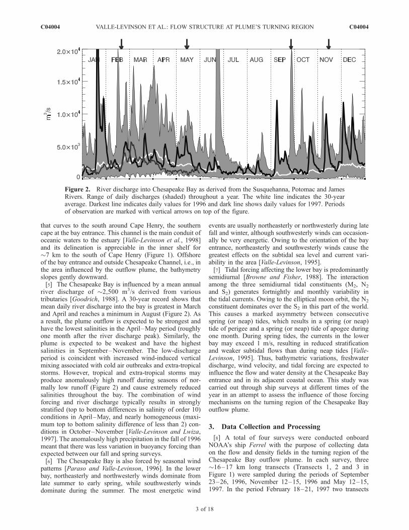
river discharge of �2,500 m3/s derived from varioustributaries [Goodrich, 1988]. A 30-year record shows thatmean daily river discharge into the bay is greatest in Marchand April and reaches a minimum in August (Figure 2). Asa result, the plume outflow is expected to be strongest andhave the lowest salinities in the April–May period (roughlyone month after the river discharge peak). Similarly, theplume is expected to be weakest and have the highestsalinities in September–November. The low-dischargeperiod is coincident with increased wind-induced verticalmixing associated with cold air outbreaks and extra-tropicalstorms. However, tropical and extra-tropical storms mayproduce anomalously high runoff during seasons of nor-mally low runoff (Figure 2) and cause extremely reducedsalinities throughout the bay. The combination of windforcing and river discharge typically results in stronglystratified (top to bottom differences in salinity of order 10)conditions in April–May, and nearly homogeneous (maxi-mum top to bottom salinity difference of less than 2) con-ditions in October–November [Valle-Levinson and Lwiza,1997]. The anomalously high precipitation in the fall of 1996meant that there was less variation in buoyancy forcing thanexpected between our fall and spring surveys.[6] The Chesapeake Bay is also forced by seasonal wind

patterns [Paraso and Valle-Levinson, 1996]. In the lowerbay, northeasterly and northwesterly winds dominate fromlate summer to early spring, while southwesterly windsdominate during the summer. The most energetic wind

events are usually northeasterly or northwesterly during latefall and winter, although southwesterly winds can occasion-ally be very energetic. Owing to the orientation of the bayentrance, northeasterly and southwesterly winds cause thegreatest effects on the subtidal sea level and current vari-ability in the area [Valle-Levinson, 1995].[7] Tidal forcing affecting the lower bay is predominantly

semidiurnal [Browne and Fisher, 1988]. The interactionamong the three semidiurnal tidal constituents (M2, N2

and S2) generates fortnightly and monthly variability inthe tidal currents. Owing to the elliptical moon orbit, the N2

constituent dominates over the S2 in this part of the world.This causes a marked asymmetry between consecutivespring (or neap) tides, which results in a spring (or neap)tide of perigee and a spring (or neap) tide of apogee duringone month. During spring tides, the currents in the lowerbay may exceed 1 m/s, resulting in reduced stratificationand weaker subtidal flows than during neap tides [Valle-Levinson, 1995]. Thus, bathymetric variations, freshwaterdischarge, wind velocity, and tidal forcing are expected toinfluence the flow and water density at the Chesapeake Bayentrance and in its adjacent coastal ocean. This study wascarried out through ship surveys at different times of theyear in an attempt to assess the influence of those forcingmechanisms on the turning region of the Chesapeake Bayoutflow plume.

3. Data Collection and Processing

[8] A total of four surveys were conducted onboardNOAA’s ship Ferrel with the purpose of collecting dataon the flow and density fields in the turning region of theChesapeake Bay outflow plume. In each survey, three�16–17 km long transects (Transects 1, 2 and 3 inFigure 1) were sampled during the periods of September23–26, 1996, November 12–15, 1996 and May 12–15,1997. In the period February 18–21, 1997 two transects

Figure 2. River discharge into Chesapeake Bay as derived from the Susquehanna, Potomac and JamesRivers. Range of daily discharges (shaded) throughout a year. The white line indicates the 30-yearaverage. Darkest line indicates daily values for 1996 and dark line shows daily values for 1997. Periodsof observation are marked with vertical arrows on top of the figure.


3 of 18

C04004

(Transects 1 and 3 in Figure 1), instead of three, weresampled because wind conditions and sea state hindereddata collection during the first day of scheduled sampling.In May 1997, Transect 2 had a different orientation than inthe other surveys in order to coordinate data sets of thatsurvey with those of COPE II experiments [e.g., Sletten etal., 1999; Hallock and Marmorino, 2002].[9] At each transect, underway measurements of current

velocity profiles and of near-surface temperature and salin-ity were obtained repeatedly for at least 24 hours of cruisingat speeds of �2.5 m/s. Transect repetitions had to bedelayed or interrupted periodically because of heavy shiptraffic through the Chesapeake Channel. Despite thosedifficulties, each transect was occupied for at least 10 timesduring the sampling period. Complementing the underwaymeasurements were profiles of temperature and salinityobtained typically at the ends of each transect repetitionand roughly in the middle or at the deepest point of thetransect.[10] Underway current velocity profiles were obtained

with a Broadband RD Instruments 600-kHz acoustic Dopplercurrent profiler (ADCP) mounted on a �1.4 m-long cata-maran. The catamaran was towed mid-ship with a three-point bridle so the catamaran traveled off the starboard sidein water undisturbed by the ship’s wake. The ADCP pointeddownward and collected current and bottom track velocities.The velocities were recorded every 4 seconds in 0.5 m binsand averaged into 30 second ensembles. This represented aspatial resolution of �75 m in the horizontal. The firstADCP bin was centered at �2 m for every survey.Navigation data were obtained with a Trimble 2000Differential Global Positioning System (DGPS) and wereused for ADCP compass calibration and current velocitydata correction as in Joyce [1989]. This data set correspondsto a total of 11 experiments, each spanning at least 24 hours,or more than 110 transect realizations. As such, this is themost comprehensive data set available for current velocityprofiles with high horizontal resolution in the turning regionof the Chesapeake Bay outflow plume.[11] The values of current velocity obtained at each

transect repetition were rotated to their axis of maximumvariance. Then they were interpolated, for each component,onto a uniform grid with horizontal and vertical resolutionsof 200 m and 0.5 m, respectively. The time series of currentvelocity components for each separate cruise was least-squares fitted to a periodic function with semidiurnal(period of 12.42 hours) and diurnal (period of 23.93 hours)constituents [e.g., Valle-Levinson et al., 1998]. This proce-dure yielded five parameters related to the flow at theentrance to Chesapeake Bay: the subtidal flow duringthe period of observation, the amplitude and phase of thesemidiurnal constituent, and the amplitude and phase of thediurnal constituent. At the bay entrance (Transect 1),the least-squares fit explained an average of 92% of thevariability observed in the principal-axis component of theflow at every grid point. The fit yielded root-mean-squarederrors between the fit and the observations that in generalremained below 0.15 m/s. The percent of variabilityexplained by the fits (or goodness of fit) decreased fromTransect 1 to Transect 2 and 3.[12] Underway near-surface (�1.5 m depth) temperature

and salinity values were obtained with a SeaBird SBE 21

thermosalinograph. The instrument was connected to theflow-through seawater system of the Ferrel. Temperatureand salinity data were combined with the DGPS signal andrecorded every 10 seconds, yielding a spatial resolution of�25 m. These data were used to construct profiles of meansurface salinity along each transect. Mean surface salinitieswere used to characterize the hydrography of the outflowplume at each transect sampled.[13] Profiles of temperature and salinity were obtained at

fixed stations of each transect with a conductivity-temperature-depth (CTD) recorder. An Applied Micro-systems EMP-2000 CTD was used in the 1996 surveysand a Seabird SBE25 was used in the 1997 surveys. CTDuse was dictated by instrument availability. During thefour surveys, profiles of temperature and salinity werecustomarily collected at each end of the transect repetitionand in the middle or at the deepest part of the transect.This approach was adopted to best characterize thehydrography data without compromising the quality ofthe towed ADCP data, because the ADCP data collectiondeteriorates every time the ship stops. The main purposeof the CTD data collection was to help discern thevertical structure of the plume.

4. Forcing Agents: Ancillary Data

[14] Ancillary data were used to characterize the forcingat the lower Chesapeake Bay and outflow plume during thesurvey periods. Ancillary data consisted of river discharge(Figure 2), wind velocity (Figure 3) and subtidal sea levelvariability (Figure 3). River discharge data were obtainedfrom the United States Geological Survey National WaterInformation System (waterdata.usgs.gov/nwis/discharge).Daily data were retrieved for the Susquehanna River atConowingo MD (01578310), for the Potomac River nearWashington DC at Little Falls Pump Station (01646500),and for the James River at Cartersville, VA (02035000). Theriver discharge values portrayed in Figure 2 represent thecombination of those three rivers, which account for �82%of the river input into the bay, for the common period1967–1997. Hourly wind velocity and sea level observa-tions were obtained from NOAA’s Chesapeake Bay BridgeTunnel station (8638863). This was the closest station to thesampling region with data available during the study period.[15] The surveys were conducted at times of the year

(vertical arrows on Figure 2) to capture the expectedseasonal variability in river discharge and wind conditions.Weak river discharge was expected in September on thebasis of daily averages across the year from the 30-yearrecord (Figure 2). Strong wind forcing was expected inNovember and February, and strong freshwater influencewas anticipated in May (Figure 2). However, 1996 was thewettest year on record for the Chesapeake Bay (blackcontinuous line on Figure 2), with daily discharge maximarecords established several times that year. The Septemberand November surveys actually took place during anoma-lously high river discharges for those months (>3000 m3/s)and after discharge peaks >10,000 m3/s (Figure 2). Theobservations in February 1997 and May 1997 occurredduring river discharges close to their respective monthlymeans and to the annual mean of 2500 m3/s (Figure 2).Because of this sustained buoyancy forcing, a well-defined


4 of 18

C04004

outflow plume was identified in every survey. The plumeitself was noticeably influenced by tides and winds.[16] The September 1996 survey took place two days

before and during spring tides, with variable winds (south-westerly to northwesterly) and subtidal sea level (Figure 3a).

The November 1996 survey was carried out followingspring tides with northwesterly and northeasterly winds thatkept subtidal sea level down (by driving water out of thebay), but allowed it to set-up during sampling of Transect 1(Figure 3b). The February 1997 survey took place at the

Figure 3. Wind velocity vectors (indicating direction toward which the wind blows), subtidal sea level,and high-pass sea level during each experiment. Shaded periods indicate measurement of a transect.


5 of 18

C04004

transition from neap to spring tides and had southwesterly,northeasterly and southeasterly winds that first caused weakset-down and then weak set-up of the subtidal sea level(Figure 3c). Finally, the May 1997 survey was conductedduring the three days leading to neap tides under variablewinds. Winds caused sea level set-down followed by set-upin Transect 1 sampling and weak subtidal sea level oscil-lations during sampling of the other 2 transects (Figure 3d).The response time of the flow to wind forcing from thenortheast and southwest in the lower bay is less than10 hours. Northeasterly winds cause unidirectional, laterallyvarying exchange flows at the bay entrance [Valle-Levinsonet al., 2001]. Northwesterly winds cause the greatest flush-ing of water out of the bay and southwesterly winds inducethe strongest bidirectional (vertically varying) exchangeflows [Valle-Levinson et al., 2001]. The variability in theseforcing agents will be discussed in the context of similaritiesand differences in the subtidal flows observed at eachtransect.

5. Data Description

[17] The description of the data set derived from thesesurveys begins with the distributions of mean surfacehydrography along each transect. It continues with the

portrayal of mean vertical profiles of salinity at differentlocations along the transects. It then presents survey-to-survey similarities and differences exhibited by the subtidalflow at each transect sampled. Throughout these descrip-tions ‘‘downstream’’ refers to the preferred direction ofcoastal current produced by the plume (Kelvin-wave sense)and ‘‘upstream’’ indicates toward the estuary’s mouth.

5.1. Mean Surface Salinity

[18] In the 3 transects sampled, the lowest overall salinityshould have been observed at Transect 1, which was closestto the source of fresh water. This was clearly the case inMay 1997, but not in the other surveys (Figure 4) becauseof dissimilar atmospheric influences during sampling ofdifferent transects. For instance, the streamwise salinitygradients in May 1997 (Figure 4d) were produced bywind-induced advection of high salinity water toward thebay entrance during Transect 3 sampling. Overall, for alltransects, the lowest salinities were observed immediatelyoff Cape Henry in Transect 1, i.e., right against the coast(distances <500 m in Figure 4). As the plume moveddownstream it seemed to have separated from the coastbecause the lowest salinity of Transects 2 and 3 wastypically found at distances >1 km (Figure 4). This locationcorresponded to that of the Chesapeake Channel and

Figure 4. Temporal mean surface salinity (upper subpanel) and streamnormal salinity gradient (lowersubpanel) drawn along each transect for all surveys. All dotted lines represent Transect 1, dark lines relateto Transect 2 and gray lines represent Transect 3.


6 of 18

C04004

suggested that, downstream of the point of separation atCape Henry, the core of the plume was largely constrainedby the channel.[19] The plume separation from shore was also observed in

the offshore, or streamnormal, gradients of the mean surfacesalinity @S/@n, where n is the streamnormal direction. Thedistributions of @S/@n showed portions with negative valuesat distances <6–8 km on Transects 2 and 3 (Figure 4). Thisindicated that salinity decreased offshore at those transectsand that the lowest salinities were observed detached from thecoast. On Transect 1, at the bay entrance, the gradient wasweak or positive near Cape Henry as the lowest salinity wasfound against the coast. These distributions around theturning region of the Chesapeake Bay outflow were consistent

with observations in Delaware Bay [Sanders and Garvine,1996]. The offshore hydrographic edge of the plume could beidentified as the location where the gradient decreasedmarkedly, after having attained high values. This plume edgelocation was somewhat ambiguous in Figure 4, but it isplausible that it was found between 10 and 14 km. Theoffshore edge of the plume as suggested by @S/@n was lessambiguous in November for transects 2 and 3 (�12 km), inFebruary for transect 3 (�13.5 km) and in May for transect 3(�13 km). This edge could have been related to the internalradius of deformation Ri, which equals (g0 H)

1=2 /f, where g0 isthe reduced gravity (in m/s2), H is the outflow plume depth(in m) and f is the Coriolis parameter (8.8� 10�5 s�1 for theChesapeake Bay entrance). To compare Ri to the observed

Figure 5. Profiles of mean salinity and vertical gradient at each location of the two transects sampled inFebruary 1997.


7 of 18

C04004

location of the plume’s edge, g0 and H were derived frommean salinity profiles.

5.2. Mean Salinity Profiles

[20] Mean salinity profiles are only shown for February1997, when the lowest salinity of the four surveys wasobserved. The vertical patterns remained consistent fromsurvey to survey when comparing transect to transect andlocation to location. The mean salinity profiles at the bayentrance (Transect 1) showed increasing salinity away fromCape Henry (Figure 5), consistent with the surface salinitydistributions. The greatest range of surface to bottom valueswas observed in Chesapeake Channel, the deepest locationsampled. Downstream of the bay entrance, the lowestsalinity in Transects 2 and 3 was observed in the channel,away from the coast (Transect 2 not available in February asportrayed in Figure 5). This location of the lowest salinitywas consistent with the mean surface distributions and alsoindicated the separation of the plume from the coast.Otherwise the lowest salinity should have been against thecoast. The vertical gradients of the salinity profiles showeda well-defined structure associated with the outflow plumeand suggested plume depths H of 5–10 m. Typical top-to-bottom salinity differences of 6 to 10 indicated g0 valuesbetween 0.05 and 0.08 m/s2. The self-advecting speeds ofthe outflow plume cp, as derived from the long internalwave speed (g0H)

1=2 were then 0.5 to 0.9 m/s, which yielded

a Ri of 7–10 km. These Ri values are conservative over-estimates (they are likely to be �7 km) on the basis ofFigure 5 results and are smaller than the offshore plumeedge suggested by hydrography. These Ri estimates willalso be compared later to plume locations indicated bysubtidal flows.[21] Another noteworthy hydrographic feature observed

in the surveys was that the highest salinities (>29) wereobserved in Chesapeake Channel (Figure 5) and offshore.This distribution suggested that offshore dense waters maketheir way into Chesapeake Bay by plunging intoChesapeake Channel and following the deepest channels.So it is likely that a substantial source of salty water to theChesapeake Bay has downstream origins, drawn by thegravitational circulation associated with the plume.

5.3. Subtidal Flows

[22] The mean flows observed during �24 hours ofsampling at each transect (Figures 6 and 7) illustrated thetransverse structure of the outflow plume. The patternsobserved at Transect 1 have already been described in detailby Valle-Levinson et al. [1998] and will not be repeatedhere. Here we focus on the patterns of subtidal flowassociated with the containment of the plume and thewithdrawal of salty waters from a downstream source, aswell as the outflow plume separating from Cape Henry. Theoutflow plume itself showed transverse structure similarities

Figure 6. Mean streamwise (contours) and streamnormal (vectors) flows at each section measured inSeptember and November 1996. Looking upstream. Shaded areas indicate upstream flow.


8 of 18

C04004

and differences from transect to transect and from survey tosurvey. Consistent patterns across all the Transect 2 and 3surveys included the development of depth-independentupstream flows throughout a 2 to 3 km-wide region nextto the coast. Other similarities were found in the area ofChesapeake Channel, as the channel: (a) mostly constrainedexchange flows; (b) contained the strongest downstreamand upstream flows; and (c) enclosed most of the outflowplume volume. Differences were distinguished in the depthat which the outflow plume felt the bottom at each transectand survey, although there were some similarities in thisaspect, too. More differences were noted in instances whenthe outflow plume remained detached from the bottom, assuggested by the patterns of downstream flow. Similaritiesand differences among subtidal flows in different transectsare now explored further, with the mean streamwise andstreamnormal flows illustrated in Figures 6 and 7.[23] A revealing pattern that arose from the surveys was

the upstream flow in the nearshore 2–3 km of Transects 2and 3. This pattern was consistent with separation of theplume noted in the mean surface and profile salinitydistributions (Figures 4 and 5) and indicated a recirculationof bay plume waters likely caused by flow separation atCape Henry. At this northern hemisphere location, Coriolisaccelerations fU, where U is a typical outflow speed, wouldtry to keep the outflow plume constrained against the coast.In contrast, centrifugal accelerations U2/R, where R is the

radius of curvature of the bathymetry off Cape Henry (�6–7 km), would try to separate the outflow from the coast. Thevalue of U at which Coriolis and centrifugal accelerationsbecome the same, or when the Rossby number equals 1, isthe product f R or 0.5 to 0.6 m/s. The outflow wasoccasionally >0.5 m/s and therefore could have separatedfrom Cape Henry. Another possible explanation for thisseparation was the asymmetric nature of tidal flows at thebay mouth, i.e., tidal rectification. During ebb, the flow islike a source potential and during flood it is like a radialsink [e.g., Chadwick and Largier, 1999]. The ebb-floodasymmetry translates into a tidal mean recirculation aroundthe cape. Whether the flow separation results from tidalrectification or from seasonal pulses of strong plume out-flow remains to be determined. Regardless of the cause, theflow separation should generate the recirculation patternobserved in all four surveys, with nearshore upstream flow(Figures 6 and 7). The recirculation around Cape Henry canbe illustrated more clearly in a vector representation(Figure 8) that showed large lateral shears in the outflownear the coast. In general, surface downstream flow devel-oped in the channel while upstream flow appeared at everydepth close to the shore. The vector representation alsoillustrated bathymetric influences on exchange flows.[24] Consistent exchange flows were also mostly found in

Chesapeake Channel during every survey at each of thethree transects sampled (Figures 6–8). These exchange

Figure 7. Mean streamwise (contours) and streamnormal (vectors) flows at each section measured inFebruary and May 1997. Looking upstream. Shaded areas indicate upstream flow.


9 of 18

C04004

flows followed the typical estuarine circulation consisting ofbuoyant, downstream flow in upper layers and denser,upstream flow underneath. This vertically sheared pattern,preferentially observed in the deepest part of each transect,contrasted to the laterally sheared pattern in which upstreamflows develop throughout the channel and downstreamflows appear over adjacent shallow areas [e.g., Wong,1994]. The observed vertically sheared pattern has beenattributed to nonnegligible Earth’s rotation effects relative tofrictional influences as characterized by the vertical Ekmannumber E [Kasai et al., 2000; Valle-Levinson et al., 2003].Earth’s rotation effects were quantified by Coriolis accel-erations fU and frictional influences could be represented by

AzU/h2, where Az is a typical kinematic eddy viscosity

(1� 10�3 m2/s) and h is a typical depth that scales U (10 m).The Ekman number was then Az/fh

2 or 0.1, which suggestedthat both Coriolis and frictional accelerations played a role inshaping the observed exchange flows. Friction was lessinfluential in the deepest areas (E depends inversely on h2)and that is why exchange flows appeared there. InChesapeake Channel, the asymmetric cross-channel distri-bution of net flows indicated that Coriolis accelerations musthave deflected net upstream and downstream flows to theirright, respectively (Figures 6–8). These bathymetricinfluences are explored with an analytical solution furtherdescribed in the Discussion.

Figure 8. Mean vectors for each survey, plotted at different depths. The figure suggests anticycloniccirculation off Cape Henry and exchange flows in Chesapeake Channel.


10 of 18

C04004

[25] The strongest downstream flows of each transectsampled were observed near the surface in the ChesapeakeChannel (Figures 6 and 7). Net plume flows were as strong as0.7 m/s (Transect 3 in November 1996 and February 1997)but also as weak as 0.05 m/s (Transects 2 and 3 in May 1997)and 0.15 m/s at the bay entrance (Transect 1). Similarly, thestrongest upstream flows preferentially appeared in thechannel at depths between 10 and 20 m. Maximuminflows of 0.3 m/s were observed at the bay entrancein February 1997 (Figure 7). Another interesting aspectthat was similar from survey to survey was that most ofthe outflow plume was constrained by the channel. Eventhough the low salinity signal may have extended beyondboth edges of the channel, the mean volume outflow waslargely delimited by those edges. The net downstreamvolume fluxes in Chesapeake Channel oscillated between�200 and 18,000 m3/s and were determined, in somemeasure, by wind forcing (Figure 9).

[26] Wind forcing, both local and remote, caused somevariability in the net flow patterns. For instance, the strongestdownstream flow and transports in Transect 3 occurred inNovember 1996 and February 1997 (Figures 6–9).These flows developed with �10 m/s northwesterly andsouthwesterly winds, respectively, with very little variabilityin their speed and direction (Figure 9). Northwesterly windsare the most efficient for flushing waters out of ChesapeakeBay and southwesterly winds are the most efficient infavoring exchange (surface outflow and inflow underneath)at the bay entrance [Valle-Levinson et al., 2001]. Eventhough the resultant wind was southwesterly during theperiod of observations of Transect 1 in May 1997, thedownstream flow and transport were very weak (Figure 9c).This was attributed to the periods of southeasterly windsbefore and during transect sampling and also, perhaps moreprominently, to the fact that subtidal sea level was increas-ing (Figure 3d). This sea level response was not directlylinked to local wind forcing and points to the importance of

Figure 9. (a) Resultant and variability of wind velocity during the period of each section measured.Positive arrows indicate northward and eastward winds. (b) Maximum net flow for each section.(c) Volume flows integrated in Chesapeake Channel.


11 of 18

C04004

remote effects in modifying both the volume exchange atthe bay entrance and the behavior of the plume. Theimportance of remote forcing on the outflow plume wasalso evident during sampling of Transect 3 in September1996. Although winds were predominantly from the north(Figures 3a and 9a), their magnitude changed markedly andtheir direction switched from northwesterly to northeasterly.In addition, sea level increased during sampling and causedvery weak downstream transports.[27] The pattern in Transect 2 changed from a robust

downstream transport in September and November of 1996to a very weak transport in May 1997. In September 1996the downstream transport was not likely driven by theobserved onshore winds (Figures 3a and 9a) but rather bya subtidal sea level drop (Figure 3a). In November 1996, thedownstream transport was likely driven by the combinationof northwesterly winds and depressed subtidal sea level(Figure 3b). The weak transport of May 1997 in Transect 2was likely the result of a rebounding stage of the plume afterthe influence of southwesterly winds the day before. Thecessation of southwesterly winds caused an increase insubtidal sea level 0.5 days before sampling. This subtidalsea level increase, together with strong southeasterly windsduring the second half of sampling, opposed the down-stream progression of the plume. The joint effects of

subtidal sea level increase and southeasterly winds couldhave caused the plume to expand offshore [e.g., Hallockand Marmorino, 2002]. Finally, the pattern in Transect 1was that of a relatively well developed outflow plume,except in February 1997, when northeasterly and southeast-erly winds combined with a subtidal sea level that wastrending up to markedly weaken the outflow plume. One ofthe main findings from these surveys was that both the localwinds and remote wind effects, as represented by subtidalsea level changes, modified the structure of the outflowplume.

6. Discussion

[28] This section centers on the (a) temporal variability ofthe subtidal flow structure, (b) bathymetric constraints to theplume and (c) recirculation characteristics at the turningregion of the Chesapeake Bay plume. The effects of riverdischarge in modulating the subtidal flow structure of theplume were not discernible in the surveys because there wasalways enough freshwater input to produce a marked plume.For these surveys, atmospheric forcing played the mostimportant role in modifying the outflow plume. The effectsof downwelling- and upwelling-favorable winds have beenrelatively well documented [e.g., Hickey et al., 2005; Chao,

Figure 10. Absolute value of the tidal average ratio between advective and Coriolis accelerations asestimated from observations. Shaded areas denote ratios < 1 (Coriolis > advective). Looking upstream.Transects measured in September and November 1996.


12 of 18

C04004

1988; Fong and Geyer, 2001; Xing and Davies, 1999].Remote atmospheric forcing, in the form of subtidal fluc-tuations in sea level h@h/@ti, should also be crucial for thefate of the plume by modulating it at its source [e.g.,Garvine, 1985, 1991]. Remote effects are proportional toh@h/@ti and are most effective when the subtidal fluctua-tions in sea level are relatively fast (�1 day) or when watercolumn stratification is relatively weak [e.g., Wong andValle-Levinson, 2002]. Similarly, Wong and Valle-Levinson[2002] found that local effects are effective when stratifi-cation is strong.[29] It has been proposed by Yankovsky and Chapman

[1997] that when stratification is strong, the plume isdetached from the bottom and is ‘surface-advected’ allow-ing it to react easily to local wind forcing. According tothem, on the basis of cyclostrophic dynamics, the plumewill be constrained within a distance Ls, given by:

Ls ¼ 2 3g0H þ u2p

� �=f 2g0H þ u2p

� �1=2; ð1Þ

where up is a typical speed of the outflow plume and H isthe plume depth as it enters the coastal ocean. For theobservations at the turning region of the Chesapeake Bayoutflow plume up attained values between 0.15 and 0.7 m/s,H was between 10 and 15 m, and g0 between 0.05 and

0.08 m/s2. Thus, predicted Ls would be between 30 and55 km, which is more than twice the various limitsobserved, and the Chesapeake Bay outflow plume wasunlikely ‘surface advected’ during the periods observed.[30] In contrast to the surface-advected plume, the plume

could remain attached to the bottom until reaching a criticaldepth hc. If hc > H and the distance at which hc is found isfarther offshore than Ls then the offshore extent of theplume would be determined by advection in the bottomboundary layer. Following Yankovsky and Chapman [1997],the critical depth is given by:

hc ¼ 2L upHf =g0� �1=2 ð2Þ

where L is the width of the estuary mouth (16 km). Takingthe range of values observed, the critical depth hc wasbetween 7 and 24 m. This suggested that the ChesapeakeBay plume may sometimes be bottom-advected (for highvalues of hc). It is essential to note, however, that in someinstances hc < H and the bottom-advected approach toestimate the offshore plume extent [Yankovsky andChapman, 1997] would not apply. This issue was addressedby Lentz and Helfrich [2002], who included bottom slope geffects. They proposed that the typical scale of the internalradius of deformation Ri, as defined in the Mean SalinityProfiles subsection, is modified by the ratio of cp, the long

Figure 11. Same as Figure 10 but for February and May 1997.


13 of 18

C04004

internal wave speed, to cg, the propagation speed over smallbottom slope and equals gg0/f. The offshore extent of theplume is then Ri (1 + cp/cg). In the Chesapeake Bay outflowregion, however, the bottom slope is not constant (see, forinstance, Figures 6 and 7) and changes sign in ChesapeakeChannel. Even so, taking values of g between 0.001 and0.003, cp between 0.5 and 0.9 m/s (Mean Salinity Profilessubsection), and cg between 0.6 and 2.7 m/s, yields ratios ofcp/cg between 0.2 and 1.5. This means that the plume iscontained within distances between 1.2 Ri and 2.5 Ri. Theobservations showed a smaller range of plume containmentthan those proposed by the above theories. Clearly, theplume core and its main outer edge were constrained byChesapeake Channel, as also suggested by Sletten et al.[1999]. It can then be proposed that the bathymetricallysteered upstream flow contributes to restrain the mainvolume of the outflow plume. Through both friction andadvection, such upstream flow should influence thedynamics and the offshore extent of the plume.[31] The effects of advection on the Chesapeake Bay

plume were discerned by comparing mean advective effects

to mean Coriolis accelerations for each transect and survey(Figures 10 and 11). Mean advective effects were approx-imated with the only advective term that could be reliablydetermined. This term was calculated from lateral flows vreconstructed from the harmonic analysis results through<v@v/@n>, where brackets denote tidal averages and nindicates streamnormal direction. Mean Coriolis effectswere calculated with the streamwise flow u and wererepresented as <fu>. The comparisons consistently showedthe importance of advective effects in Transects 1 and 2, atthe turning region of the plume. In those transects, theabsolute value of the ratio <v@v/@n> / <fu> was mostly >1,which suggested that Coriolis accelerations may not havebeen dominant in that region. Further downstream, atTransect 3, Coriolis accelerations became clearly prevalent.This difference can also be seen in the increasing impor-tance of Coriolis accelerations when Transect 2 wasreoriented further downstream in the May 1997 survey. Itwas also seen that the outflow plume could separate fromCape Henry when the velocity exceeded the product of theCoriolis parameter and the radius of curvature f R, i.e., when

Figure 12. Observed along-isobath flows (a through d in cm/s) in Transect 3 compared to model resultswith observed bathymetry (e through h in cm/s) and flat bottom (i through l, at transect’s mean depth).Model results were obtained by prescribing the following parameters: (e) and (i) Az = 0.0014 m2/s,R = 7000m3/s upstream; (f) and (j)Az = 0.001m

2/s, R = 16000m3/s downstream; (g) and (k)Az = 0.0006m2/s,

R = 11000 m3/s downstream; (h) and (l) Az = 0.0017 m2/s, R = 12000 m3/s upstream. Prescribed transportswere within 10% of the net transports calculated from observations for each case. Sea level slopes wereN = 1 � 10�6 {1 + i exp[�(y/B � 1)2]} (see Appendix A).


14 of 18

C04004

centrifugal accelerations exceeded Coriolis accelerations.By Transect 3, R becomes large (relatively straight isobaths)and therefore a much larger velocity is required beforeadvection becomes important.[32] The influence of bathymetry, and the friction related

to its variability, on the plume structure could be exploredwith a linear solution [e.g., Kasai et al., 2000; Valle-Levinson et al., 2003]. The solution arises from a simplifieddynamic balance among pressure gradient (both barotropicand baroclinic), Coriolis acceleration and friction. Theshape of the solution describing exchange flows (given inAppendix A) depends on the prescription (a) of a sea level

slope, (b) of a space-independent eddy viscosity Az, and(c) of net transports through the section. The exchangepatterns arising from solution A3 showed very good agree-ment with those observed in Transect 3 (Figure 12). Theresemblance was striking at distances >3.5 km, whichindicated that the main dynamics in most of the transectwas well captured by a linear approach. In transect 3(Figure 12), advective accelerations were weakest and thatis why the comparison is so favorable. At the other 2transects, where advective effects were more prominent,comparable exchange flow patterns can still be reproduced[e.g., Valle-Levinson et al., 2003]. Solutions over flat-

Figure 13. Surface vectors interpolated onto a uniform grid. Even though this figure does not portray asynoptic picture because of the changing winds from one day to another, all representations depictanticyclonic circulation over the shallow area off Cape Henry.


15 of 18

C04004

bottom bathymetry, with the same forcing as that used toproduce the results of Figure 12, showed a markedly differentplume and upstream flow structure. The model-observationsagreement underlined the importance of bathymetry in con-straining the upstream flow and the outflow plume. It isnoteworthy that the Delaware River plume, for instance,shows analogous bathymetric steering [e.g., Munchow andGarvine, 1993] whereas the Hudson River plume is uncon-strained by bathymetry in the vicinity of the outflow (R. J.Chant et al., manuscript in preparation, 2007). Both theChesapeake andDelaware channels tend to steer the estuarineoutflow along the coast and may favor coastal currentformation. In contrast, the lack of bathymetric steerage ofthe Hudson’s outflow may play a role in the tendency for itsdischarge to form a large unsteady bulge [Choi and Wilkin,2007; R. J. Chant et al., manuscript in preparation, 2007]. Ingeneral, it can be postulated that plumes constrained bychannels will produce coastal currents (in the Kelvin-wavesense), while unconstrained plumes will be more reactive towind forcing and prone to bulge formation.[33] The recirculation (upstream flow) observed in the

Chesapeake Bay outflow within the 3.5 km closest to thecoast was not explained by solution A3 (Figure 12). Thiswas because of the nonlinear character of the recirculation,which was associated with flow separation at Cape Henry.The flow separation caused the formation of two boundariesfor the plume waters, one offshore and one inshore, duringebb periods. This was analogous to observations in Dela-ware Bay [Sanders and Garvine, 1996] and from radarmeasurements in the Chesapeake Bay [Sletten et al., 1999]and ADCPs [Marmorino et al., 2000; Marmorino andTrump, 2004]. During flood periods, the flow is like apotential sink [e.g., Chadwick and Largier, 1999] andmoves in roughly the same direction as in ebb (toward thebay mouth) in the region inshore of the ChesapeakeChannel. This resulted in net flows moving downstreamin the channel and upstream inshore of the channel. Themean anticyclonic recirculation was clearly illustrated byforming surface maps from interpolated values of eachtransect (Figure 13). Even though these representationscould not provide a truly synoptic picture of the surfaceflow field because of the rapidly changing forcing condi-tions, even from day to day, they did show a recirculation.This is owing to the persistent and coherent flow toward thebay mouth in the region inshore of the channel. Whether theobserved anticyclonic recirculation around Cape Henrydevelops under much weaker riverine inputs than thoseobserved in this study remains a question to be explored.Nonetheless, it is hypothesized that the recirculation is mostlikely caused by tidal rectification as also suggested byJohnson [1976], Marmorino et al. [2000] and Marmorinoand Trump [2004]. The persistent observations of thisanticyclonic recirculation in different studies suggests addi-tional observational or modeling studies to explore whetherit functions as a retention mechanism for transport of larvaethat require re-entrance into Chesapeake Bay for theirsurvival.

7. Conclusion

[34] This observational study at the turning region of theChesapeake Bay outflow plume has produced revealing

results. Centrifugal accelerations combine with frictionalinfluences to produce an anticyclonic recirculation off CapeHenry and also, through bathymetric variations, to limit theoffshore extent of the plume. The mean downstream flowrelated to the plume is mostly constrained by the edges ofChesapeake Channel. This channel provides and importantpathway for coastal ocean water to enter into ChesapeakeBay underneath the plume.

Appendix A: Model

[35] The model that generated the results of Figure 12solves for the nontidal or mean along-isobath u and trans-verse v flows produced by pressure gradients and modifiedby Coriolis and frictional influences. In a right-handedcoordinate system (x, y, z), where x points downstream, yoffshore and z upward, the nontidal (or steady) momentumbalance to be solved becomes a set of two differentialequations:

�fv ¼ �g@h@x

þ g

r@r@x

zþ Az

@2u

@z2

fu ¼ �g@h@y

þ g

r@r@y

zþ Az

@2v

@z2

ðA1Þ

where f, g, ro, r, h, Az are the Coriolis parameter, the gravityacceleration (9.8 m/s2), reference water density, variablewater density (kg/m3), surface elevation (m), and verticaleddy viscosity homogeneous in z and y (m2/s), respectively.The set of equations (A1) may be represented in terms of acomplex velocity w = u + iv, where i 2 = �1 is the imaginarynumber:

gN � Dz ¼ Az

@2w

@z2� i f w: ðA2Þ

In (A2), N and D represent the barotropic and baroclinicpressure gradients, respectively:

N ¼ @h@x

þ i@h@y

D ¼ g

r@r@x

þ i@r@y

� �

and are assumed independent of depth. Then, the flow w hascontributions from the sea level slope and from thehorizontal density gradients, i.e.,

w zð Þ ¼ gNF1 zð Þ þ F2 zð Þ ðA3Þ

and F1 and F2 represent functions that depict the verticalstructure of the barotropic (from sea level slope) andbaroclinic (from density gradient) contributions to the flow.Using equation (A3), then equation (A2) can be rewrittenas:

@2F1

@z2� i f

Az

F1 ¼1

Az

@2F2

@z2� i f

Az

F2 ¼ �Dz

Az

: ðA4Þ


16 of 18

C04004

Assuming, as boundary conditions, no stress at the surface(@F1/@z = @F2/@z = 0 at z = 0), and no-slip at the bottom (F1

and F2 = 0 at z = �Hy), and that the horizontal densitygradient is independent of depth, the solution of (A4) is:

F1 ¼i

f1� cosh azð Þ

cosh aHy

� �" #

F2 ¼iD

f aeaz � azð Þ � e�aHy � aHy

� � cosh azð Þcosh aHy

� �" # ðA5Þ

In this solution, the parameter a equals (1 + i)/DE, where DE

is the Ekman layer depth [2Az/f]1=2. Solutions (A5) and (A3)

require prescription of the sea level slope N and the eddyviscosity Az and a density gradient D that is dynamicallyconsistent with N. In order to derive the value of D we use aboundary condition that assumes a prescribed net volumeflux R (m3/s) along or across a cross-section [Kasai et al.,2000], i.e.,

ZB0

Z0

�Hy

w dz dy ¼ R ðA6Þ

where B is the estuary’s width. The value of D that satisfiesa prescribed N is:

D ¼

R f a2 � iagI1

ZB0

N yð Þd y

iI2

¼(R f a2 � iag

ZB0

N yð Þ e�aHy þ aHy

� �tanh aHy

� ��

� 1� e�aHy þ a2H2y =2

� �idy

)

�(i

ZB0

tanh aHy

� �� aHy

� �dy

)�1

ðA7Þ

Prescribing N (= 1 � 10�6 {1 + i exp[�(y/B � 1)2]}), Az

(order 10�4 to 10�3 m2/s), R, and Hy (as any function of y),the solution to (A3) is obtained with (A5) and (A7) andportrayed in Figure 12. The shape of N was justified byobservations as described by Valle-Levinson et al. [2003].

[36] Acknowledgments. This work was funded by the U.S. MineralManagement Service under cooperative agreement 14-35-001-30807 andby the NOAA Office of Sea Grant, under grant R/CF-47 to the VirginiaGraduate Marine Science Consortium and Virginia Sea Grant CollegeProgram. Ship time on the NOAA ship Ferrel was provided by the NationalSea Grant College Program. We greatly appreciate the professional supportand cooperation from the crew of the Ferrel under the able command ofLCDR S. D. McKay. We also appreciate the technical support of R. C. Kiddand L. Brasseur plus the participation of T. Royer, J. Klinck, R. Ellison,E. Haskell, G. Jiang, J. Koziana, T. McCarthy, M. Moore, S. Paraso,B. Parsons, C. Reiss, C. Reyes, D. Ruble, S. Wathanaprida, B. Wheless,M. Gruber, S. East, and S. Kibler on various surveys. We appreciate thecomments of A. Yankovsky and one anonymous reviewer who helpedimprove the presentation of the paper.

ReferencesAvicola, G., and P. Huq (2002), Scaling analysis for the interaction betweena buoyant coastal current and the continental shelf: Experiments andobservations, J. Phys. Oceanogr., 32, 3233–3248.

Boicourt, W. C. (1981), Circulation in the Chesapeake Bay entrance region:Estuary-shelf interaction, in Chesapeake Bay Plume Study: Superflux1980, edited by J. Campbell and J. Thomas, NASA Conf. Publ., 2188,61–78.

Browne, D. R., and C. W. Fisher (1988), Tide and tidal currents in theChesapeake Bay, NOAA Tech. Rep. NOS OMA 3, 84 pp., Natl. Oceanicand Atmos. Admin., Rockville, Md.

Chadwick, D., and J. Largier (1999), Tidal exchange at the bay-oceanboundary, J. Geophys. Res., 104, 29,901–29,924.

Chao, S. Y. (1988), River-forced estuarine plumes, J. Phys. Oceanogr., 18,72–88.

Chao, S. Y., and W. C. Boicourt (1986), Onset of estuarine plumes, J. Phys.Oceanogr., 16, 2137–2149.

Choi, B. J., and J. L. Wilkin (2007), The effect of wind on the dispersal ofthe Hudson River plume, J. Phys. Oceanogr., in press.

Fong, D. A., and W. R. Geyer (2001), The response of a river plume duringan upwelling favorable wind event, J. Geophys. Res., 106, 1067–1084.

Fong, D. A., W. R. Geyer, and R. P. Signell (1997), The wind-forcedresponse of a buoyant coastal current: Observations of the western Gulfof Maine plume, J. Mar. Syst., 12, 69–81.

Garvine, R. W. (1985), A simple model of estuarine subtidal fluctuationsforced by local and remote wind stress, J. Geophys. Res., 90, 11,945–11,948.

Garvine, R. W. (1991), Subtidal frequency estuary-shelf interaction: Ob-servations near Delaware Bay, J. Geophys. Res., 96, 7049–7064.

Garvine, R. W. (1995), A dynamical system of classifying buoyant coastaldischarges, Cont. Shelf Res., 15, 1585–1596.

Garvine, R. W. (2001), The impact of model configuration in studies ofbuoyant coastal discharge, J. Mar. Res., 59, 193–225.

Goodrich, D. M. (1988), On meteorologically induced flushing in threeU.S. east coast estuaries, Estuarine Coastal Shelf Sci., 26, 111–121.

Hallock, Z. R., and G. O. Marmorino (2002), Observations of the responseof a buoyant estuarine plume to upwelling favorable winds, J. Geophys.Res., 107(C7), 3066, doi:10.1029/2000JC000698.

Hallock, Z. R., P. Pistek, J. W. Book, J. L. Miller, L. K. Shay, and H. T.Perkins (2003), A description of tides near Chesapeake Bay entranceusing in situ data with an adjoint model, J. Geophys. Res., 108(C3),3075, doi:10.1029/2001JC000820.

Hickey, B. M., S. L. Geier, N. B. Kachel, and A. MacFadyen (2005), A bi-directional river plume: The Columbia in summer, Cont. Shelf Res., 25,1631–1656.

Johnson, R. E. (1976), Circulation study near Cape Henry, Virginia, usingLagrangian techniques, Tech. Rep. 21, 80 pp., Inst. of Oceanogr., OldDominion Univ., Norfolk, Va.

Joyce, T. M. (1989), On in situ calibration of shipboard ADCPs, J. Atmos.Oceanic Technol., 6, 169–172.

Kasai, A., A. E. Hill, T. Fujiwara, and J. H. Simpson (2000), Effect of theEarth’s rotation on the circulation in regions of freshwater influence,J. Geophys. Res., 105, 19,961–19,969.

Kourafalou, V. H., L.-Y. Oey, J. D. Wang, and T. N. Lee (1996), The fate ofriver discharge on the continental shelf: 1. Modeling the river plume andthe inner shelf coastal current, J. Geophys. Res., 101, 3415–3434.

Lentz, S. J., and K. R. Helfrich (2002), Buoyant gravity currents along asloping bottom in a rotating fluid, J. Fluid Mech., 464, 251–278.

Marmorino, G. O., and C. L. Trump (2000), Gravity current structure of theChesapeake Bay outflow plume, J. Geophys. Res., 105, 28,847–28,861.

Marmorino, G. O., and C. L. Trump (2004), Evolution of the Cape Henryfront, Estuaries, 27, 389–396.

Marmorino, G. O., L. K. Shay, B. K. Haus, R. A. Handler, H. C. Graber,and M. P. Horne (1999), An EOF analysis of HF Doppler radar currentmeasurements of the Chesapeake Bay buoyant outflow, Cont. Shelf Res.,19, 271–288.

Marmorino, G. O., T. F. Donato, M. A. Sletten, and C. L. Trump (2000),Observations of an inshore front associated with the Chesapeake Bayoutflow plume, Cont. Shelf Res., 20, 665–684.

Miller, J., M. Goodberlet, and J. Zaitzeff (1998), Remote sensing of salinityin the coastal zone, Eos Trans. AGU, 79, 173, 176–177.

Munchow, A., and R. W. Garvine (1993), Dynamical properties of abuoyancy-driven coastal current, J. Geophys. Res., 98, 20,063 –20,077.

O’Donnell, J., G. O. Marmorino, and C. L. Trump (1998), Convergenceand downwelling at a river plume front, J. Phys. Oceanogr., 28, 1481–1495.

Oey, L.-Y., and G. L. Mellor (1993), Subtidal variability of estuarine out-flow, plume, and coastal current: A model study, J. Phys. Oceanogr., 23,164–171.


17 of 18

C04004

Paraso, M. C., and A. Valle-Levinson (1996), Meteorological influences onsea level and water temperature in the lower Chesapeake Bay: 1992,Estuaries, 19, 548–561.

Ruddick, K. G., E. Deleersnijder, P. J. Luyten, and J. Ozer (1995), Halinestratification in the Rhine-Meuse freshwater plume: A three-dimensionalmodel sensitivity analysis, Cont. Shelf Res., 15, 1597–1630.

Sanders, T. M., and R. Garvine (1996), Frontal observations of the Dela-ware Coastal Current source region, Cont. Shelf Res., 16, 1009–1021.

Shay, L. K., T. M. Cook, Z. R. Hallock, B. K. Haus, H. C. Graber, andJ. Martinez (2001), The strength of the M2 tide at the Chesapeake Baymouth, J. Phys. Oceanogr., 31, 427–449.

Simpson, J. H., and A. J. Souza (1995), Semidiurnal switching of stratifica-tion in the region of freshwater influence of the Rhine, J. Geophys. Res.,100, 7037–7044.

Sletten, M. A., G. O. Marmorino, T. F. Donato, D. J. McLaughlin,and E. Twarog (1999), An airborne, real aperture radar study ofthe Chesapeake Bay outflow plume, J. Geophys. Res., 104, 1211–1222.

Stern, M. E., J. A. Whithehead, and B. L. Hua (1982), The intrusion of adensity current along the coast of a rotating fluid, J. Fluid Mech., 123,237–265.

Valle-Levinson, A. (1995), Observations of barotropic and baroclinicexchanges in the lower Chesapeake Bay, Cont. Shelf Res., 15, 1631–1647.

Valle-Levinson, A., and K. M. M. Lwiza (1997), Bathymetric influences onthe hydrography of the lower Chesapeake Bay, J. Mar. Syst., 12, 221–236.

Valle-Levinson, A., C. Li, T. Royer, and L. Atkinson (1998), Flowpatterns at the Chesapeake Bay entrance, Cont. Shelf Res., 18,1157–1177.

Valle-Levinson, A., K. Wong, and K. Bosley (2001), Observations of thewind-induced exchange at the entrance to Chesapeake Bay, J. Mar. Res.,59, 391–416.

Valle-Levinson, A., C. Reyes, and R. Sanay (2003), Effects of bathymetry,friction and Earth’s rotation on estuary/ocean exchange, J. Phys.Oceanogr., 33, 2375–2393.

Whitehead, J. A., and D. C. Chapman (1986), Laboratory observations of agravity current on a sloping bottom: The generation of shelf waves,J. Fluid Mech., 172, 373–399.

Wong, K.-C. (1994), On the nature of transverse variability in a coastalplain estuary, J. Geophys. Res., 99, 14,209–14,222.

Wong, K. C., and A. Valle-Levinson (2002), On the relative importance ofthe remote and local wind effects on the subtidal exchange at the entranceto Chesapeake Bay, J. Mar. Res., 60, 477–498.

Xing, J., and A. M. Davies (1999), The effect of wind direction and mixingupon the spreading of a buoyant plume in a non-tidal regime, Cont. ShelfRes., 19, 1437–1483.

Yankovsky, A. E., and D. C. Chapman (1997), A simple theory for the fateof buoyant coastal discharges, J. Phys. Oceanogr., 27, 1386–1401.

��R. J. Chant, Institute of Marine and Coastal Sciences, Rutgers University,

New Brunswick, NJ 08904, USA.K. Holderied, NOAA, Kasitsna Bay Laboratory, Homer Office, 2181

Kachemak Drive, Homer, AK 99603, USA.C. Li, Coastal Studies Institute, Louisiana State University, Baton Rouge,

LA 70803, USA.A. Valle-Levinson, Department of Civil and Coastal Engineering,

University of Florida, 365 Weil Hall, Gainesville, FL 32611, USA.([email protected])


18 of 18

C04004

subtidal flow structure at the turning region of a wide...

Documents