NBER WORKING PAPER SERIES

SUBSIDIZING LOW- AND MIDDLE-INCOME ADOPTION OF ELECTRIC VEHICLES: QUASI-EXPERIMENTAL EVIDENCE FROM CALIFORNIA

Erich MuehleggerDavid S. Rapson

Working Paper 25359http://www.nber.org/papers/w25359

NATIONAL BUREAU OF ECONOMIC RESEARCH1050 Massachusetts Avenue

Cambridge, MA 02138December 2018, Revised January 2021

We gratefully acknowledge research funding from the State of California Public Transportation Account and the Road Repair and Accountability Act of 2017 (Senate Bill 1) via the University of California Institute of Transportation Studies. We thank Tom Knox at Valley Clean Air Now and Mei Wang at South Coast Air Quality Management District for sharing their expertise on the pilot programs in San Joaquin Valley and South Coast, respectively; the California Air Resources Board for their support of this project and for funding for acquisition of some of the data used in this analysis; Jim Archsmith, Ben Dawson, Jack Gregory, Tyler Hoppenfeld and Shotaro Nakamura for excellent research assistance; and many seminar participants. The views expressed herein are those of the authors and do not necessarily reflect the views of the California Air Resources Board or the National Bureau of Economic Research.

NBER working papers are circulated for discussion and comment purposes. They have not been peer-reviewed or been subject to the review by the NBER Board of Directors that accompanies official NBER publications.

© 2018 by Erich Muehlegger and David S. Rapson. All rights reserved. Short sections of text, not to exceed two paragraphs, may be quoted without explicit permission provided that full credit, including © notice, is given to the source.

Subsidizing Low- and Middle-Income Adoption of Electric Vehicles: Quasi-Experimental Evidence from CaliforniaErich Muehlegger and David S. RapsonNBER Working Paper No. 25359December 2018, Revised January 2021JEL No. H22,H23,H71,L62,Q48,Q55,Q58,R48

ABSTRACT

Little is known about electric vehicle (EV) demand by low- and middle-income households. In this paper, we exploit a policy that provides exogenous variation in large EV subsidies targeted at the mass market in California. Using transaction-level data, we estimate three important policy parameters: the rate of subsidy pass-through, the impact of the subsidy on EV adoption, and the elasticity of demand for EVs among low- and middle-income households. Demand for EVs in our sample is price-elastic (-3.3) and pass-through to buyers is indistinguishable from 100 percent. We use these estimates to calculate that the expected subsidy bill required for California to reach its goal of 1.5 million EVs by 2025 is likely to exceed $12-18 billion.

Erich MuehleggerDepartment of EconomicsUniversity of California, DavisOne Shields AvenueDavis, CA 95616and NBERemuehlegger@ucdavis.edu

David S. RapsonDepartment of EconomicsUniversity of California, DavisOne Shields AvenueDavis, CA 95616dsrapson@ucdavis.edu

A data appendix is available at http://www.nber.org/data-appendix/w25359

1 Introduction

Electrification of the vehicle fleet is seen by many policy-makers as central to reducing green-

house gas emissions, local air pollution and dependence on oil. Local, state and national

governments have set ambitious targets for widespread adoption of electric vehicles (EVs) or

phasing out internal combustion engines (ICEs) entirely. In recent years, countries announcing

plans to ban ICEs sales include France and UK (by 2040), Norway (by 2025), India (by 2030),

and China. Germany has announced plans to put 1 million electric vehicles on the road by

2020. In the U.S., California is leading the charge. In 2013, Governor Brown issued an execu-

tive order to put 1.5 million so-called “Zero Emissions Vehicles” (ZEVs) on the road by 2025

(and 5 million by 2030) as part of a goal to reduce transportation emissions by 50 percent by

2030. To spur adoption, policy-makers pair these targets with generous subsidy programs. The

cost of these programs is considerable and presents stark tradeoffs for public funds. As of mid-

2020, California has spent nearly $900 million on the state-wide vehicle subsidies, and recent

proposals suggested allocating another $3 billion in the state. Federal incentives for electric

vehicles total up to $1.5 billion per manufacturer.

Although a long literature estimates the impact of incentives for hybrid, electric or alternative-

fuel vehicles,1 research on past programs may not provide a good guide as to the impact or fis-

cal costs of meeting these ambitious targets for two reasons. First, past incentives for alternative

vehicles rarely offer the quasi-experimental variation necessary for clean causal identification.

In virtually all cases, the decision to offer an incentive is endogenously determined. States with

populations predisposed to purchase EVs are more likely to offer incentives, confounding esti-

mation of the causal impact of incentives on vehicle adoption. Second, and equally important,

the ambitious targets described above require widespread adoption of electric vehicles.2 Yet,

past incentive programs typically offered a blanket subsidy to all vehicle buyers, the take-up

of which is strongly correlated with income. As Borenstein and Davis (2016) documents, high

income households were significantly more likely adopt EVs and claimed the vast majority of

federal vehicle incentives, and the income distribution of subsidy recipients has not changed

over time.3 As such, elasticities derived from early adoption may be less relevant for assess-

ing the impacts or costs of policies or targets that require widespread adoption of alternative

1e.g., Chandra et al. (2010), Gallagher and Muehlegger (2011), Beresteanu and Li (2011), Clinton and Steinberg (2017)study effects on adoption, Sallee (2011), Gulati et al. (2017) study pass-through and recent papers, including Li et al.(2017), Li (2017), Springel (2017), study network effects of charging stations.

2Mary Nichols, Chair of the California Air Resource Board, noted in Jan 2018 that that the 2030 market share of EVsin California would have to be approximately 40% to meet the 5 million by 2030 goal (Los Angeles Times).

3https://energyathaas.wordpress.com/2019/05/13/an-electric-vehicle-in-every-driveway/

2

fuel vehicles. Given the imminence of major policy decisions relating to these targets and trans-

portation emissions reductions in general, there is an urgent need to better understand demand

for EVs in the mass market.

In this paper, we study the impacts of the Enhanced Fleet Modernization Program (“EFMP”),

a California retire-and-replace subsidy program for EV purchases that addresses both of the

challenges above. The design of the EFMP provides clean quasi-experimental variation in the

availability of the subsidy to some buyers and not others, allowing for a transparent treatment-

to-control comparison. Furthermore, subsidy eligibility is means-tested, directing subsidies

specifically towards low- and middle-income buyers. This allows us the opportunity to esti-

mate the elasticity of demand for EVs for a sub-population that has not, historically, adopted

electric vehicles, but will be an important market for meeting ambitious policy targets.

We analyze the universe of electric vehicle sales in California, a state that accounts for 40

percent of EV purchases in the United States and 10 percent of purchases worldwide. Using

difference-in-difference, matched diff-in-diff and triple-differenced models that exploit geo-

graphic, temporal and subsidy-exposure variation, we retrieve estimates of three policy-relevant

parameters: the rate of subsidy pass-through for the program, the impact on EV adoption and

the elasticity of demand for EVs among low- to middle-income buyers. Low- and middle-

income buyers capture the majority of the subsidy, consistent with the intentions of program

designers. Each of these is essential for understanding the effectiveness of public expenditures

on demand-side EV subsidies. In all of our specifications, the rate of subsidy pass-through is

close to 100 percent, and in no specification can we reject full pass-through. In addition, we

find that low- and middle-income buyers are relatively responsive to the subsidies. In each

of our specifications, the estimated demand elasticity is within a tight range between -3.2 and

-3.4, implying that a subsidy that decreases the buy-price of an EV by 10 percent will increase

demand for that EV by 32-34 percent. While this may seem like a large effect at first glance, the

small baseline quantity implies that even a large elasticity translates into a modest number of

additional EVs.

Together, and under assumptions about generalizability, these objects can be combined to

estimate the magnitude of subsidy funds that would be required to achieve a policy goal along

the lines of “put 1.5 million ZEVs on the road”. Under optimistic estimates of the baseline (no-

subsidy) rate of EV growth in California going forward, we place the likely required subsidy

bill at no less than $12-$18 billion for a program that would subsidize new EVs.4 The mag-

4We view this as a lower bound as a result of having made conservative assumptions throughout that would, if any-thing, lead this number to be too low. Moreover, our estimates of demand elasticity are large relative to the literature,

3

nitude of the estimated subsidy bill is large, and may compel California regulators to explore

policy alternatives. A mandate or a “feebate” would shift the burden of the policy away from

California taxpayers, although these have very different implications for economic efficiency.

The burden on California taxpayers will also be affected by a continuation or cancelation of the

existing federal EV tax credit that is presently being reconsidered.

While we are encouraged to offer an estimate of the EV demand elasticity in California

that is retrieved using quasi-experimental variation, context is required for those who wish to

extrapolate these results. The suitability of these estimates for general use as demand elastici-

ties may differ by setting (construct validity). Subsidy eligibility under the EFMP is linked to

having a car to scrap, and is also driven by targeted marketing efforts by program administra-

tors, particularly in one of the pilot regions. Moreover, the program does not exist in isolation,

which is a feature common to all EV elasticity estimates in the literature to date. The presence

of large federal and state subsidies for new EVs affects the interpretation of results since many

of the new EVs purchased under a given subsidy program (in our case EFMP) were eligible for

other state-wide or federal EV subsidies as well. Moreover, the ZEV Mandate – a policy requir-

ing manufacturers to sell a certain proportion of EVs in California and nine other participating

states – implicitly subsidizes manufacturers who sell EVs. While our empirical design nets

out effects of statewide and federal demand-side subsidies as well as supply-side programs,

the extent to which our elasticity estimates (which reflect marginal subsidy changes) apply to

ranges of prices on the inframargin is an open question.

Notwithstanding these caveats, this paper makes several new contributions to the state of

knowledge about the market for EVs. First, we provide (to our knowledge) the first estimates

of the EV demand elasticity that are supported by a treatment-versus-control empirical design

that allows key identifying assumptions to be tested directly. Second, ours is (again, to our

knowledge) the first paper to examine EV adoption amongst low- and middle-income house-

holds that form the bulk of the market and will be central to meeting ambitious EV targets.

Third, our estimates of subsidy pass-through contribute to the literature on the incidence of

vehicle incentives. Fourth, we use our elasticity and incidence estimates to offer the first esti-

mate of the range of subsidies required to meet California’s 2025 EV adoption targets grounded

by causal identification. This contributes to an important contemporary policy debate that is

likely to be repeated in jurisdictions across the globe in coming years.

and the subsidy bill is inversely related to the demand elasticity.

4

2 Institutional Details and Data

The Enhanced Fleet Modernization Program is a vehicle incentive program in California that

provides subsidies to low- and middle-income households to scrap old vehicles for newer (al-

though in some cases, still used), cleaner and more fuel efficient vehicles.5 The EFMP was ini-

tially designed as a retire-and-replace program along the lines of cash-for-clunkers.6 In April

2015, the California Air Resources Board (“ARB”) redesigned the program to combine fea-

tures of a retire-and-replace program with an incentive program for the purchase of high fuel

economy vehicles and EVs, targeting low- and middle-income consumers in disadvantaged

communities (“DACs”). 7 The redesigned program, the focus of this paper, was launched as a

pilot in July 2015 in two Air Quality Management Districts (“AQMDs”): the San Joaquin Valley

Air Pollution Control District and the South Coast Air Quality Management District. Over the

first two years, the pilot program received $72 million in state funding with the expectation to

expand the program to other metro areas.8

2.1 Subsidy eligibility and generosity

The pilot program is restricted to participants residing in the two AQMDs and retiring a qual-

ifying vehicle.9 Within the AQMD, the EFMP targets: (a) households living in or near “disad-

vantaged” communities and (b) low- and middle-income households at or below 400% of the

federal poverty line.10

To participate in the program, households must reside in a designated “disadvantaged

community”. The disadvantage designation is determined by the California Enviornmen-

tal Protection Agency (“CalEPA”). At the census-tract-level, CalEPA calculates a CalEnviro-

Screen (“CES”) score that aggregates traditional measures of socio-economic disadvantage

(e.g., poverty and unemployment), measures of pollution exposure (e.g., ambient air pollution

levels and the presence of clean-up and solid waste sites) and sensitivity to pollution (e.g., child

5EFMP is a distinct program from the Clean Vehicle Rebate Program (“CVRP”), the main consumer-facing alterna-tive vehicle incentive program in California that is available state-wide and, until recently, was available to all privatebuyers of qualified vehicles.

6See Mian and Sufi (n.d.), Li et al. (2013) for analyses examining the effects of the federal Cash-for-Clunkers program.7https://www.arb.ca.gov/msprog/aqip/efmp/finalregulationorder2014.pdf8ARB is in negotiation with three new AQMDs (Bay Area AQMD, Sac Metro AQMD, San Diego AQMD) to expand

the program.(see. e.g., https://www.arb.ca.gov/board/books/2017/062217/17-6-1pres.pdf). If expanded, ninety per-cent of “disadvantaged communities” (described further below) in California will be covered by the EFMP.

9Vehicles must be: (1) a light-duty vehicle, (2) registered and insured for the two previous years, (3) with relativelyhigh emissions, defined by the AQMD.

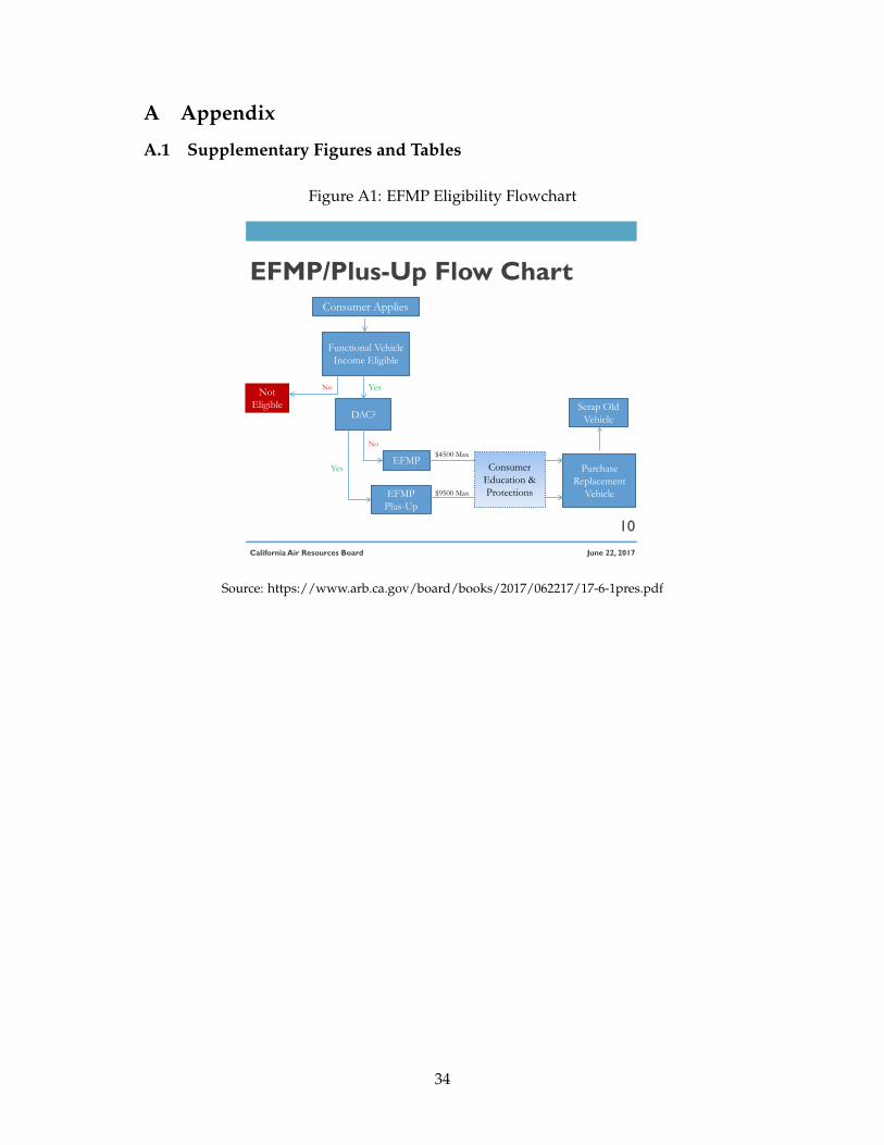
10Appendix figure A1 illustrates a flowchart for eligiblity.

5

and elderly share of the population) at the census-tract level.11 CalEPA classifies all census

tracts with CES score in the top quartile of the state-wide CES distribution as a disadvantaged

census tract. To qualify for the EFMP program, a household must reside in a “disadvantaged

zip code”, a zip code that (wholly or partially) contains a disadvantaged census tract. We refer to

these “‘disadvantaged zip codes” as disadvantaged communities (“DACs”).

Within these DACs, the program is means-tested with lower income households eligible

for more generous incentives. Households below the 225% of the FPL are eligible for the most

generous incentives: $5,000. As household income rises, subsidy generosity declines until a

household is no longer eligible for the program, above 400% of the federal poverty line. Table

1 lists the subsidies that we study in this paper, which are available for program participants

who trade in their vehicle for an electric vehicle.12

Figure 1 maps zip code boundaries for the Southern two-thirds of California. Regions in

grey are the San Joaquin Valley and South Coast AQMDs, the two AQMDs that piloted the

EFMP over our study period. The zip codes in pink are those that contain a disadvantaged

census tracts. Thus, means-tested households in zip codes that are both grey and pink would

be eligible for the subsidy. Outside of the grey and pink boundaries of the two participating

AQMDs and disadvantage zip codes, households would be ineligible.

Figure 2 plots the histogram the maximum CES score within a zip code for participating

AQMDs (right panel) and non-participating AQMDs (left panel). The vertical red line in each

plot marks the 75th percentile of state-wide CES score Zip codes to the right of the red line

would be classified as disadvantaged communities by the rules of the program. Roughly 80

percent of the population of the San Joaquin Valley ACMD and South Coast AQMD live in zip

codes classified as DACs.

2.2 Additional EFMP implementation details

The ARB sets general rules for the pilot program which administrators must follow. In both

South Coast and San Joaquin Valley, the AQMDs are responsible for administering the pro-

gram and determining household eligibility. In addition, the AQMDs must build a network

of participating dealerships that agree to a set of consumer protections, including “no-haggle”

posted prices, limitations on dealership financing, required information provision and inspec-

11Appendix figure A2 summarizes the components of the CES score.12The EFMP program also offers subsidies of approximately equal magnitude that are available according to slightly

different rules and eligibility criteria, but do not rely on the DAC designation. These are netted out in our empiricaldesign and are not used to identify our parameters of interest.

6

tion for used vehicles.

But, the ARB granted each district substantial latitude with respect to implementation, and

specifically, marketing, outreach and the application process. In the South Coast AQMD, infor-

mation about the program is relayed through marketing and participants apply online. After

the AQMD determined an applicant is eligible, the program directs the applicant to contact the

list of pre-approved dealerships. In San Joaquin Valley, the program is administered through

regular “Tune-in and Tune-up” events on weekends and other direct outreach events through-

out the San Joaquin Valley, specifically targeting minority groups. Eligible buyers are then

guided through the application process and, if eligible, are directed towards the websites of

participating dealerships.

2.3 Data and summary statistics

We merge three datasets: (1) disadvantaged community designations available from CalEPA,

(2) program rebate data and (3) transaction-level data on the universe of new and used EVs

purchased by California buyers.

The DAC designations are publicly available at the census tract level.13 Following the pro-

gram rules, we map census tracts to zip codes and classify a zip code as disadvantaged if it

contains part or all of a disadvantaged census tract. The EFMP rebate data are publicly avail-

able at the transaction-level. For each transaction the data report value of the subsidy, the

vehicle purchased and the zip code in which the recipient of the subsidy lives. Our vehicle

transaction data was purchased from a major market research firm. For the universe of bat-

tery electric vehicles (“BEVs”) and plug-in hybrid vehicles (“PHEVs”) purchased by buyers in

California, we observe the make, model and model-year of the vehicle, the transaction price

as reported to the Department of Motor Vehicles, the zip code of the buyer and the dealership

that sold the vehicle.

We summarize transaction counts, prices and subsidies in table 2, grouping zip codes by

whether they are in or out of the participating pilot regions (AQMD = 1) and whether they are

classified as a disadvantaged zip code (DAC = 1). Roughly half of the population of Califor-

nia resides in the participating AQMDs, of which the majority live in communities classified

as disadvantaged for purposes of the AQMD pilot program. Outside of the pilot regions, a

higher fraction of the population lives in non-disadvantaged zip codes, reflective of higher in-

comes and the fact that the South Coast AQMD and the San Joaquin Valley are locations with

13See https://oehha.ca.gov/calenviroscreen/report/calenviroscreen-version-20

7

relatively poor air quality.

Buyers in disadvantaged zip codes purchase less expensive and fewer EVs on a per capita

basis, before and after the start of the EFMP pilot. Yet, foreshadowing our empirical results, per

capita EV sales rise most quickly in disadvantaged zip codes in the participating AQMDs. That

said, EFMP transactions are a small fraction of overall EV sales. In disadvantaged communities

during the pilot program, roughly two percent of the transactions received an EFMP subsidy.14

Consistent with the construction of the disadvantaged community identifier, these commu-

nities are less-advantaged along a number of sociodemographic indicators. In the first three

columns of Table 3, we present population-weighted average demographics for all of Cali-

fornia (column 1), disadvantaged communities outside the pilot regions (column 2) and dis-

advantaged communities outside the pilot regions (column 3). Relative to all of California,

households in disadvantaged communities tend to have households incomes that average ten

to fifteen thousand dollars lower than the mean household in California, are less likely to have

graduated from high school, are more likely to be Hispanic or African American and are more

likely to be unemployed. Yet, relatively to the averages for California, disadvantaged com-

munities are less unusual than the set of zip codes associated with EV adoption through 2018.

In column 4, present the summary statistics weighting by historical EV sales. Consistent with

the evidence from Borenstein and Davis (2016), the sociodemographics of zip codes of early

adopters of EVs suggest these zip codes are a particularly advantaged subset of California,

with mean incomes roughly thirty-five thousand dollars higher than the average California

household, higher educational attainment and lower rates of unemployment.

3 Methodology

The features of EFMP program lend themselves to a difference-in-differences specification com-

paring disadvantaged in and out of the two participating AQMDs, before and after the start of

the pilot program.15 We can extend this to include an additional difference, by including the

non-disadvantaged communities in and out of the participating AQMDs. Using this frame-

work, we estimate three policy parameters of interest: (1) the incidence of the EFMP subsidies

and (2) impact of the EFMP incentives on electric vehicle adoption, and (3) the elasticity of

14We do observe a small number of subsidies (rough 2% of the total) provided to households that, according to thesubsidy data, live in zip codes that are not classified as disdvantaged.

15While the discontinuous nature of disadvantaged community assignment might suggest a regression discontinuitydesign is appropriate, the means-testing of the program causes most of the relevant variation to occur well away fromthe discontinuity. This can be seen in Appendix Figure A4.

8

demand for alternative fuel vehicles, specifically amongst low- and middle-income customers

targeted by the EFMP.

We aggregate our transaction-level data to the zip-quarter, the finest level of temporal and

spatial disaggregation for which we have subsidy data, and the geographic level of treatment

assignment.16 We consider a zip code as treated if the zip code is located in the South Coast or

San Joaquin Valley Air Quality Management Districts (“AQMD=1”), contains at least part of

one DAC census tract (“DAC=1”) and the calendar date is in the third quarter of 2015 or later

(“Post=1”).

3.1 Difference-in-differences specification

To retrieve a difference-in-differences estimate of the intent-to-treat effect of the incentive on

the price paid by the buyers or the impact on EV sales, comparing disadvantaged communities

in and out of the pilot regions, one could estimate

Yzt = α11A1P + νtA + γz + εzt (1)

where Yzt is the dependent variable of interest, 1A and 1P are indicators for AQMD=1 and

Post=1, respectively. Zip code and AQMD-by-quarter-by-year effects are conditioned out via

γz and νtA. Here, the coefficient α1 reflects an estimate of the intent-to-treat for buyers in

disadvantage zip codes in the pilot region.

In our context, the magnitude of α1 will depend mechanically on the proportion of EV

transactions that receive the EFMP subsidy. As noted in table 2, even in the treated zip codes,

the number of EFMP subsidies is small, on average, relative to the total number of EV sales.

Thus, we anticipate the intent-to-treat estimates to be equivalently small as they reflect the

average of a few treated transactions with many transactions for which the subsidy was not

claimed. We construct a continuous treatment variable, λzt, to be the fraction of EV purchases

that receive an EFMP subsidy in each zip-quarter.

λzt =∑i 1(Subsidyizt > 0, zip = z, time = t)

∑i 1(zip = z,time = t)(2)

Using λzt as a continuous treatment in place of the treatment dummy in (1), we estimate

16The data on EFMP reports the quarter of purchase and the owner’s zip code, but does not provide the VehicleIdentification Number (“VIN”) of the purchased vehicle. Thus, we cannot match information on EFMP subsidies toexact transactions in the purchase data. Rather, we observe the mean EFMP subsidy received by EVs purchased byhouseholds at the zip-quarter level.

9

the treatment-on-treated, β1. Intuitively, this scales up the intent-to-treat estimate α1 to reflect

that λzt fraction of the transactions in each zip-quarter that are affected by the EFMP program.

It is reflected in equation (3):

Yzt = β1λzt + νtA + γz + εzt (3)

3.2 Matched and triple-differenced specifications

Retrieving an unbiased causal estimate from the difference-in-difference specification requires

parallel pre-trends and the absence of omitted variables correlated with the treatment in the

post-period. Figure 3 plots trends in the residual purchase price of electric vehicles, after con-

ditioning on make*model*mode-year fixed effects (left panel), and the log of EV sales (right

panel) in disadvantaged zip codes in and out of the pilot regions over time. In each graph, the

red lines and shading corresponds to the means and standard errors for disadvantaged com-

munities in the participating AQMDs; the blue lines and shading plot the analogous values

for disadvantaged communities in non-participating AQMDs. In both cases, the pre-trends

are statistically indistinguishable. The slight different in the pre-trends for residual purchase

prices as modest in comparison to the value of the EFMP incentives.

Our empirical context allows for two additional specifications to further address potential

concerns with pre-period trends (despite the fact that the pre-trends for log-quantity are close

to parallel) and omitted variables correlated with the treatment. Although the classification

for disadvantaged communities applies identically to both the pilot and non-pilot regions, the

histograms of CES scores plotted in Figure 2 indicate that the upper tail of CES scores in partic-

ipating AQMDs does not overlap with the non-participating AQMD distribution. The highest

CES score outside of the participating AQMDs (South Coast and San Joaquin) is 59.9, corre-

sponding to the 75th percentile of CES scores in the participating AQMDs. If pre-trends differ

for disadvantaged zip codes with extremely high CES scores relative to disadvantaged zip

codes outside of the participating AQMDs, our estimates will be biased. Additionally, if adop-

tion or pricing for zip codes in the very upper tail of the CES distribution changes for reasons

unrelated to the EFMP program, the differences-in-differences specification may mis-estimate

the treatment effect.

As a refinement to the difference-in-difference specification above, we use nearest-neighbor

matching to pair disadvantaged zip codes in participating AQMDs with “control” disadvan-

taged zip codes in non-participating AQMDs. We match based on the pre-period trends in av-

erage prices or quantities, following the synthetic control literature (e.g. Abadie and Gardeaz-

10

abal (2003), Abadie et al. (2010)).17

We also consider a triple-differenced specification that leverages the non-disadvantaged

communities in both the pilot and non-pilot regions, and includes a full-set of interaction fixed

effects, νtA, φtD and γz, capturing shocks common to the pilot region, shocks common to dis-

advantaged communities and time-invariant zip-level differences.

Yzt = β1λzt + νtA + φtD + γz + εzt (4)

Relative to the unmatched and matched difference-in-difference specifications above, the

triple-differenced specification controls for unobservable shocks to EV adoption or prices com-

mon to all zip codes within the pilot region. In our context, such shocks might arise if electric

vehicles became more popular throughout a pilot region due to a local policy change affecting

both advantaged and disadvantaged zip codes. If such a shock affected disadvantages and

non-disadvantaged zip codes, the triple-differenced approach will net out the impact of the

local policy change.

3.3 Instrumental Variables

In the purchase data, we do not observe which specific transactions received subsidies. Hence,

our primary variables of interest are the EFMP-share of total transactions and the average sub-

sidy across all transactions. Both are constructed by normalizing by the total quantity of EVs

in a zip*quarter. As total transactions are the denominator of our scaled variables of interest,

we would expect the OLS coefficient to be biased downward in log-quantity regressions.

We address this by instrumenting for the EFMP-share and for average subsidies in our main

specification. We instrument for EFMP-share using linear and quadratic values of the count of

EFMP-subsidized transactions in zip z at time t, normalized by mean number of transactions

in that zip for the ten quarters up until the start of the pilot program.18

As we report in our regression tables, the instrument is sufficiently strong - zip codes with

high adoption in the pre-period tend to have higher levels of adoption in the post period. And

by construction, the denominator of the instrument is constant for each zip code and hence,

uncorrelated with idiosyncratic shocks to log quantities in the post-treatment period. We report

17We plot the mean residual purchase price and the mean of log of EV sales (right panel) in the matched sample inA5.

18Formally, denoting the number of periods before the start of the pilot program as T, the quarter in which the EFMPprogram becomes active as t∗ and number of transactions in zip z in quarter t as Qzt, we construct the instrument forEFMP-share as IVzt =

EFMP Subsidy Countzt∑r<t∗ Qzr/T .

11

both the first-stage f-statistics and the Sargan-Hansen p-values for the instruments.

4 Results

4.1 Pass-through of EFMP subsidies

Our first parameter of interest is the pass-through of the EFMP incentives to buyers. Cost

effectiveness of the program is determined in part by the extent to which the subsidy affects the

price paid by the consumer, rather than accruing to dealerships or manufacturers. To estimate

incidence of the incentives, we must first describe how the composition of EVs affects our

empirical approach.

As discussed above, we aggregate our data to the zip-quarter level, as that is the finest

level of aggregation for which the subsidy data are available. It is also the geographic level

of assignment to treatment. However, the EFMP program offers incentives for households to

purchase both new and used EVs. This shifts the composition of vehicles purchased in response

to the program.19 Consequently, the mean price for all vehicles purchased in a zip-quarter

reflects both the incidence of the program and any compositional shift induced by the incentive.

To control for compositional changes and to isolate the pass-through of the incentive, we

condition on the mix of vehicles purchased in a zip-quarter by regressing transaction-level

vehicle prices on model*model-year*year-of-purchase fixed effects, odometer reading in miles

and a dummy variable reflecting whether or not the vehicles was leased. Formally, denoting

vehicle, zip, model, model year and year-quarter of purchase as i, z, m, y and t respectively, we

regress:

SellPriceizmyt = αmyt + β1Odometeri + β2Leasei + µzt + εi (5)

where SellPriceizmyt is the transaction price of the vehicle i received by the seller. In this context,

µzt captures whether dealerships in a particular zip code received more or less than the state-

wide average for vehicles of identical make and model-year (e.g., 2015 Nissan Leaf) purchased

in the same quarter and year (e.g., first quarter of 2017). Interpretation of the pass-through

regressions is a bit more straightforward using the price buyers paid net of subsidies as the de-

pendent variables. Thus, we net out the average subsidy in zip z and time t to construct our

19Although the EFMP data does not report the vehicle VIN, the public data does record the model year of the pur-chased vehicle. Roughly 80 percent of vehicles have models years more than one year less than the calendar year inwhich they are purchased, suggestive that they are used, rather than new vehicles. In contrast, 87 percent of all EVs inthe transaction data would be classified as used by this definition.

12

dependent variable:

ResidualBuyPricezt = µzt − EFMPzt (6)

where EFMPzt is the average EFMP subsidy received in the zip-quarter. Intuitively, ResidualBuyPrice

reflects whether buyers in the zip-quarter paid more or less that the statewide average, net of

any subsidies received.

We estimate two specifications that capture slightly different measures of pass-through.

First, we regress our dependent variable on the fraction of sales that received an EFMP subsidy

in a zip-quarter:

ResidualBuyPricezt = β1λzt + νtA + γz + εzt. (7)

The estimate of β1 measures the change in the price paid for vehicles by recipients of the EFMP

subsidy, relative to buyers of the same model and vintage who did not receive the EFMP sub-

sidy.20 We also estimate the pass-through directly on the price paid by buyers directly via the

following equation:

ResidualBuyPricezt = γ1EFMPzt + νtA + γz + εzt. (8)

We interpret the coefficient γ1 as the fraction of the subsidy captured by buyers as opposed to

dealers or other upstream market participants. Table 4 displays results from equations (7) in

the top panel and (8) in the bottom panel. For each, the first three columns present the OLS

estimates for the difference-in-difference, the matched difference-in-differences and the triple-

differenced specifications respectively. Columns 4 through 6 recreate these specifications using

our preferred instrument.

We find relatively consistent evidence that consumers capture the majority of the subsidy.

Relative to an average subsidy close to $5,000, our OLS results suggest that buyers with the

subsidy pay $2,954 to $3,715 less for a vehicle, net of the subsidy, relative to non-participants

purchasing the same make, model and model-year elsewhere in California. After instrument-

ing, the effect on prices rises modestly. We estimate EFMP subsidies reduce the price to the

buyer, net of subsidies, by an average of $4,673 to $5,304.

These results are echoed in panel B, which presents our estimates of the rate of subsidy pass-

through. We find that buyers capture the majority of the subsidy, between 57 and 76 percent of

the subsidy in the OLS specifications and between 94 to 108 percent in the IV specifications. In

20By construction, the average residual buy price in a zip-quarter is given by, ResidualBuyPricezt = λzt(P0 − S) +(1− λzt)P0 = P0 − λztS, where P0 and S denote the price paid by non-recipients and the dollar value of the subsidyreceived by the EFMP recipient. Estimating (7), β1 provides an estimate of S.

13

all cases, the pass-through estimates are indistinguishable from full pass-through, suggesting

that consumers capture the lion’s share of the subsidy and consistent with stated efforts on

the part of program designers who sought to channel most of the subsidy dollars to buyers

rather than sellers or upstream market participants. Our pass-through estimates are consistent

with previous work examining the pass-through of earlier hybrid vehicles subsidies. Gulati

et al. (2017) finds that new vehicle buyers with access to subsidies capture 80 to 90 percent of

the value of an incentive.21 But, unlike earlier subsidy programs that were widely available,

the EFMP program pilot was limited in scope. Although we find evidence that consumers

captured the vast majority of the benefits of the pilot program, the pass-through of a widely

implemented program might differ.

4.2 Impact of EFMP subsidies on adoption

We use similar specifications to estimate the response of demand to the program replacing

ResidualBuyPricezt with the log-quantity of sales as the dependent variable in equations (7)

and (8).

Table 5 shows the effect of the EFMP subsidies on the quantity of EVs transacted. As with

the price regressions, we present OLS estimates in columns 1 through 3, for the difference-in-

differences, matched difference-in-differences and triple differenced specifications respectively,

and IV results in columns 4 through 6.

In panel A, we regress log quantities on the fraction of EFMP sales and interpret the esti-

mated coefficient as the percentage change in EV sales resulting from EFMP program expo-

sure moving from zero to 100 percent eligibility. Our OLS results suggest that zip codes in

which all buyers were eligible for the program would experience, on average, a 26 percent

(= 100x(exp(0.23) − 1)) increase in the quantity of new EVs purchased relative to zip codes

with zero program eligibility. The point estimates are similar across the three specifications, as

we would anticipate given the relatively similar pre-trends in log quantities graphically pre-

sented in Figure 3.

As we note in the discussion of the instrument above, the structural endogeneity created

by quantity appearing on both the right and left-hand sides would bias the OLS estimate of

EFMP on sales downwards. The IV results in columns 4 through 6 confirm this. The preferred

21Gulati et al. (2017) further finds that subsidy-eligible buyers are more likely to choose vehicle options that increasethe purchase price of the vehicle, and thus pay a higher purchase price, unadjusted for options. In our case, we do notobserve the options purchased by customers. However, EFMP buyers are substantially more likely to purchase usedEVs, where the set of potential options is more limited. Moreover, unobserved options would tend to bias our estimatestowards zero, suggesting, if anything our results understate the fraction of the subsidy captured by consumers.

14

IV point estimates are more than double the OLS estimates, at .64 to .69 log-points for the un-

matched and matched difference-in-differences specifications, respectively. The bottom panel

presents estimates of the percentage change in EV sales from offering a $1,000 subsidy. In our

IV specifications, we estimate a $1,000 subsidy increases adoption by 0.13 to 0.14 log-points.

4.3 Elasticity of demand for electric vehicles

Finally, we are interested in estimating the elasticity of demand for EVs. This is of particular

interest as estimates of the elasticity of demand for early adopters reflect the price sensitivity

of primarily high-income households. In contrast, the EFMP program specifically targets low

and middle-income households that form the bulk of the population and potentially play an

important role in wide-scale adoption of EVs.

We approach this in two ways. First, we can use the estimates from tables 4 and 5 to back

out the elasticity of demand of EFMP-eligible buyers as:

εPQE

=φ

βPE. (9)

where β is the fraction of the subsidy captured by buyers and φ is an estimate of the impact of

a $1,000 subsidy on demand for EVs. 22

Assuming complete pass-through (100%) and the impact of a $1,000 subsidy (0.13) from

column 4 of Tables 4 and 5, and the average price of eligible vehicles in EFMP locations, we

have an estimate of the elasticity of demand for EFMP-eligible buyers, εPQE≈ − 0.17

1.00 ∗ 26 = −3.4.

Alternatively, we can estimate the elasticity directly by regressing log quantity on the per-

cent premium or discount at which EVs were sold in the zip-quarter. Formally, we estimate:

Log(Qzt) = β %Premium + νtA + γz + εzt (10)

where %Premium is calculated as ResidualBuyPricezt normalized by mean price of EVs in our

data. As in earlier specifications, we present both the OLS estimates and the IV estimates.

Table 6 presents elasticity estimates obtained directly from the regressions, which vary in a

tight range from -3.2 to - 3.3, depending on specification. Across all methods, our estimates are

larger than recent estimates in the literature for the elasticity of early adopters.23 This suggests

that low- and middle-income buyers are more price elastic than higher-income earlier adopters.

22See appendix section A.3 for the derivation.23Li et al. (2017) uses gasoline prices as an IV and estimates a demand elasticity of -1.3. Springel (2017) and Li (2017)

both use BLP IVs to retrieve estimates of -1.0 to -1.5 (Springel) and -2.7 (Li), respectively.

15

4.4 Supplementary results

4.4.1 Effects by air district

We do not separately estimate the effects by AQMD in our main results. Yet, program rules

allow each air district flexibility in the operation of the pilot program. Although ARB rules

specify the incentive generosity schedule and set general guidelines related to dealership par-

ticipation, the districts choose to how to market the program, handle applications and coordi-

nate with participating dealerships.

The program in South Coast operates largely through its online presence, with a relatively

modest amount of targeted marketing. Interested consumers apply on-line, at which time the

air district verifies that they have a eligible trade-in. After being pre-approved, they contact a

participating dealership and select a vehicle. The air district then confirms that the vehicle is

eligible for the incentive (i.e., not subject to recalls), that the financing meets program require-

ments, and that the household has not participated in the program previously. If approved, the

air district contacts the dealership and the transaction is completed, with the buyer paying the

price of the vehicle less the EFMP incentive.

In contrast, the program in San Joaquin engages in direct marketing to low-income and

minority households. During the study period, entry into the program occurred exclusively

through in-person attendance at local “Tune-in, Tune-up” smog testing events.24 “Tune-in,

Tune-up” events occur every couple of weeks, and rotate between regional population centers

in the San Joaquin Valley. Interested individuals bring their current vehicle to an event, re-

ceive a free smog check and, if eligible for the program, receive in-person guidance on how to

apply. At the same time, program officials verify applicant eligibility and guide the potential

participant through the application process. After the event, officials follow up with poten-

tialy applicants to help them complete their application. Once pre-approved, households are

directed to dealership websites, all of which are required to post “no-haggle” prices (e.g., Car-

max). Pending approval of a final selection by the air district, the transaction is completed and,

as in South Coast, the buyer pays the price of the vehicle less the EFMP incentive.

Table 7 presents the results allowing the coefficients of interest to vary by air district. The

four left-most columns report the OLS and IV results for prices, and the four right-most columns

report the OLS and IV results for log quantities. All columns are based on the triple-differenced

specification.

When disaggregating by AQMD, the average treatment effect on price is larger in San

24Since the end of the study period, program officials in the San Joaquin Valley have begun to take online applications.

16

Joaquin Valley than in South Coast. These differences may reflect the greater guidance to-

wards “no-haggle” dealerships with posted online prices given to program participants in the

San Joaquin Valley. However, the differences are not large enough in magnitude to be statisti-

cally distinguishable. Likewise, point estimates for pass-through rates are higher in both the

OLS and IV specifications for San Joaquin Valley, although again, the point estimates are not

statistically distinguishable across the two regions, nor are individual pass-through estimates

statistically distinguishable from complete pass-through of the subsidies to buyers.

Columns 5 through 8 present the results for EV sales. Again, the point estimates for the

effect on sales are slightly higher for San Joaquin Valley compared to South Coast, although

again, the estimates are statistically indistinguishable. We estimate that each $1,000 in subsidy

increases EV adoption by 9 and 16 percent in South Coast and San Joaquin Valley, respec-

tively. Although again, the point estimates are statistically indistinguishable, the higher point

estimate for the San Joaquin Valley program might reflect the more intensive marketing and

guidance provided by the program administrators.

4.4.2 Price effect on non-participants

An implicit assumption in the analysis above is that the EFMP does not affect the price paid

by individuals living in the program areas who were not eligible through, for example the

program acting as a shock to aggregate demand. Put formally and ignoring fixed effects for

simplicity, the mean residual buy price, by construction, is an average of the price for recipients

(fraction λzt) and non-recipients (fraction 1 - λzt). Denoting the price for non-recipients, P0 and

the dollar value of the subsidy captured by a recipient, we can denote the average price as:

ResidualBuyPricezt = λzt(P0(λzt)− S) + (1− λzt)P0(λzt) = P0(λzt)− λztS. (11)

If we regress ResidualBuyPricezt on a constant and λzt, as in:

ResidualBuyPricezt = α + β̂1λzt + νzt, (12)

and dP0(λzt)dλzt

> 0, our specification would overestimate the true change in the sales price net of

subsidies paid by program participants.

Two features of our context suggest that the relationship between P0 and λ is unlikely to

significantly bias our estimates of pass-through and the amount of the subsidy captured by the

consumer. First, the fraction of buyers who receive the EFMP is small—in “treated” zips, two

17

percent of vehicles on average receive an EFMP subsidy. Thus, the impact of the program on

the prices paid by non-participants is likely to be modest. Second, our level of analysis is at the

zip-quarter level despite the fact that zip codes themselves are not isolated markets. Rather,

these zip codes are part of large metro areas across which people purchase vehicles. Vehicles

commonly flow between metro areas in response to local supply and demand conditions. If

the program led to a substantial increase in the prices paid by non-participants within the zip

code, market forces would tend to arbitrage away a local premium for a specific vehicle. Thus,

we consider it unlikely that the small fraction of buyers who receive EFMP subsidies have a

meaningful impact on the prices paid by the vast majority of buyers who do not.

Yet, the details of the program allow us to test for spillover effects directly by examin-

ing the effect of EFMP-induced demand on prices in zip codes outside the participating air

quality districts. We implement this by restricting the sample to sales outside the participat-

ing regions and collapsing the data to quarter-of-sample by make/model-year observations.

We then regress the average residual sales price on the share of vehicles purchased under

the EFMP in that quarter. Conceptually, we compare average prices for make/model-years

popular amongst EFMP buyers to those unpopular amongst EFMP buyers. If the treatment

influences the prices paid in non-participating regions, we would expect the average prices of

popular models to increase in non-participating regions after the start of the EFMP program

relative to the prices of unpopular models.

PMMYt,AQMD=0 = αsMMY

t + XMMYt + εMMY

t (13)

In equation 13, MMY differentiates vehicles based on make and model-year, and the quarter-

of-sample is denoted by t. The coefficient of interest is α, which will be positive if the statewide

share of MMY cars sold under the EFMP program increases the price of those cars in non-

participating regions.

We find that a small but statistically insignificant effect exists. The change in sMMYt from

zero to one represents a shift from zero percent to 100 percent of MMY vehicles being sold

under the EFMP program. Our estimate shows that this would, on average, increase the trans-

action prices by $4,486. Adjusting for the share of EVs sold under EFMP (1.2 percent overall),

this implies an average increase of $53 for each such vehicle sold in non-participating AQMDs.

Adjusting instead by share of used EVs sold under EFMP (3.5 percent), it would imply an

average increase of $157 per vehicle in non-participating AQMDs.

The existence of these effects implies that the “true” treatment effect on EV prices reported

18

in Table 4 may be slightly overstated, and one may wish to adjust these coefficients towards

zero by $50-$150 when interpreting these results. The qualitative and policy implications are

unaffected, however, as these spillover effects are one-to-two orders of magnitude smaller than

the average treatment effect on treated vehicles. Moreover, the presence of these market ad-

justments reflects the efficiency with which vehicle markets operate.

5 Policy Discussion

Estimates of the demand elasticity and rate of subsidy pass-through are important policy pa-

rameters to any jurisdiction considering EV subsidies. A present-day example is the state of

California, which is currently in the legislative process that will determine the next allocation

of state EV rebate funds intended to push the state across the target goal of 1.5 million EVs on

the road by 2025. The demand elasticity and rate of subsidy pass-through are central to the

question of how much funding would be required to achieve this goal. As table 3 illustrates,

the demographics of disadvantaged zip codes are much closer to the mean demographics in

California than the demographics of the zip codes in which electric vehicles were purchased

through the end of 2017. If reaching the ambitious EV adoptions targets necessitates wider-

spread adoption than historical experience, this paper’s evidence on the impact of incentives

on lower-income communities provides an important guide.

There are several policies that reduce the retail price of EVs, including federal tax incentives,

state consumer subsidies and supply-side policies like California’s ZEV mandate, only some

of which impose a direct fiscal cost on the state budget of California. As it is difficult to predict

the exact form of state and federal subsidies in the future, we present a back-of-the-envelope

calculation intended to approximate the total cost across all sources of subsidies that apply to

purchases of new EVs going forward.25

By the end of 2017 there were roughly 330,000 EVs on the road in California. The subsidy-

inclusive growth rate in the California EV fleet can be retrieved directly from the data. It was

over 80 percent in 2014 and has steadily declined to 33 percent in 2017. In order to reach 1.5

million EVs in California by 2025, a 20.8 percent annual growth rate from 2018-2025 is required,

after taking scrappage into account.26 In order to estimate the subsidy bill required to reach

25To be clear, an implicit assumption of this exercise is that the EFMP subsidy pass-through rate would be reflectiveof the pass-through rate of a much larger program. If a larger program had a lower pass-through rate, arising fromperhaps sellers who anticipate that many buyers will have access to the subsidy, the necessary budgetary cost wouldincrease.

26The rate of used EVs exported to other states or countries, totaled in accidents, or scrapped due to old age or lackof use are each determinants of the number of EVs that will, at any point, be on the road.

19

1.5 million EVs by 2025, it is necessary first to establish a no-subsidy baseline growth rate

that would be expected to occur from 2018 - 2025 in the absence of subsidies. This is easily

retrieved using the demand elasticity estimated earlier. Finally, we use our elasticity estimates

again to calculate how much the purchase price of EVs would have to decline to shift from

the no-subsidy baseline growth rate to the necessary 20.8 percent average growth rate. This

procedure requires some assumptions, which we now describe.

The baseline rate of EV demand growth is a function of factors such as consumer prefer-

ences, relative prices and attributes of vehicles (e.g. battery range), the price of fuel inputs

(gasoline versus electricity), macroeconomic and credit conditions, and many other potential

considerations. The raw growth rate has been influenced by the presence of major subsidy

programs, both federally and at the state level. In order to net out these subsidies and retrieve

a no-subsidy baseline growth rate, we proceed under several conservative assumptions.27 We

assume a retrospective average new EV price of $35,000, and $10,000 in cumulative state and

federal subsidies captured by consumers. Based on the preferred demand elasticity of -3.3 from

our empirical estimates, we estimate no-subsidy growth rates in 2015, 2016 and 2017 of 32.3,

24.3 and 20.8 percent, respectively (Table A1). These reflect the growth rate that would have

occurred if state and federal incentives had not been present. Based on the historical pattern of

new technology adoption, one would expect that the growth rate will continue to decrease over

time as the market becomes more saturated. Therefore, we conjecture that a baseline growth

rate between 2018 and 2025 of roughly 12 to 14 percent is conservative (again in the sense that

it will likely be even lower, which would lead to even higher estimates of the subsidy require-

ment, all else equal).

Projecting forward, we need to make further assumptions about the vehicles purchased

under a subsidy program and the rate at which on-road EVs exit the California fleet, either

through accidents, exports out of California or scrappage. The subsidy program that we project

is broadly consistent with the major existing subsidy programs – the California CVRP and the

U.S. federal EV tax credit. Both of these programs offer subsidies for new EV purchases. To

align this thought exercise most closely to our empirical results, we assume the going-forward

(2018-2025) price of new EVs declines to $26,000, which is roughly the weighted average price

received by sellers for the mix of vehicles purchased under the EFMP program. An average

sale price of $26,000 is consistent with industry projections for entry-level EV models in 2025.

27Throughout this section, “conservative” is intended to describe an assumption that will lead to an under-estimateof the implied subsidy bill to achieve 1.5 million EVs by 2025. For example, a “conservative” assumption would leadto a higher baseline growth rate, thus reducing the subsidy bill requirement.

20

This subsidy bill calculation is therefore consistent with a program that only applies to new

vehicle purchases, similar to CVRP. We assume that 10 percent of the EV stock will be retired

each year starting in 2020, capturing vehicle retirements, accidents and exports to other states

and countries.

Table 8 presents the implied total value of EV subsidies that would be required for Califor-

nia to have 1.5 million EVs on the road by 2025.28 The table presents the subsidy bill estimates

for various assumed levels of annual baseline growth in the EV stock in the range of 10 to 16

percent between 2018-2025. The implied required change in buy-price is retrieved by assuming

a list price of $26,000 per EV and applying estimates of the subsidy elasticity of demand to the

implied required percent change in quantity.

Moving left-to-right, the columns assume higher baseline growth rates. Given the rate of

historical decline in growth (which is natural in rapidly-growing markets), an expected annual

growth rate of 12-14 percent from 2018-2025 seems to us to be plausible and even optimistic.

Moving from top-to-bottom in the table, the demand elasticities are increasing and we assume

demand to exhibit constant elasticity throughout this range. The top row elasticity of -2.0 re-

flects the middle of the range of elasticity estimates from the literature. The elasticity estimated

in this paper is in the range of -3.2 and -3.3, with -3.3 reflected in the bottom row.

As baseline growth rates increase, the necessary change in the price of new EVs and the

cumulative subsidy bill both decline. This reflects a diminished need for policy intervention

in order to achieve a given target EV adoption goal. The implied change in prices and subsidy

bill also declines if we assume that demand is more elastic, such that a subsidy of a given value

has a greater impact on the rate of EV adoption, all else equal.

Together, these estimates reflect the need for a substantial EV subsidy bill. Given our con-

servative approach to assumptions, the subsidy bill estimates presented in the table should be

interpreted as lower bounds. In no scenario presented here is the estimated subsidy bill floor

below $7.7 billion. Moreover, the underlying parameters support a wide range of possible sub-

sidy bills that extends well above $20 billion. The range implied by our elasticity estimates

and that correspond to 12-14 percent baseline growth is no less than $12 to $18 billion dollars.

Given that our elasticity estimates in this paper are larger than those published in the exist-

ing literature, one may wish to know the subsidy bill estimated from a smaller elasticity. An

elasticity of -2.0 implies a subsidy bill floor in the range of $18.0 to $26.9 billion dollars from

2018-2025. The presence of federal subsidies, or implicit subsidies such as the ZEV mandate,

28A more detailed description of the methodology used for these estimates can be found in Appendix section A.4.

21

would reduce the amount for which California would be directly responsible.29

6 Conclusion

In this paper we exploit variation arising from rules governing the availability of EV subsidies

in California. Using a unique dataset of both transaction prices and subsidy levels, we estimate

the elasticity of demand amongst low- and middle-income households and the fraction of the

subsidy captured by consumers. It is difficult to estimate these statistics in a credible way when

examining many of the other EV rebate policies that have been available in the California and

the United States in recent years. Both the federal EV tax credit and the California Clean Vehicle

Rebate Program subsidies were (until recently) available to any EV buyer in their jurisdiction,

making it difficult to construct a credible control group.

The rules governing the EFMP Plus Up program in California are well suited to deploying

a triple-difference methodology in program evaluation. When we do, we estimate a subsidy

elasticity of EV demand of -3.3, and a subsidy pass-through rate of 100 percent. Assuming that

these statistics are generalizable, we use them to estimate the cumulative amount of additional

subsidy dollars that will be required for California to meet its goal of having 1.5 million EVs on

the road by 2025. Depending on the assumed baseline (no-subsidy) growth rate, our estimates

imply that at least $12 - $18 billion in total subsidies will be required.

One contribution of this paper is the relevance of our estimates to low- and middle-income

households. While most EVs to date are owned by wealthy households, mass electrification of

the transportation sector will require adoption in the mass market. The means-testing and geo-

graphic targeting of the EFMP allow a rare opportunity to study the adoption decisions of low-

and middle-income buyers, whose demand and price sensitivity may be lower than those of

high income households. One instructive comparison is to benchmark our elasticity estimate

of -3.3 against implied elasticities from the earlier literature on hybrid vehicle incentives that

likely reflect the responsiveness of higher income, early adopters. Gallagher and Muehlegger

(2011) and Chandra et al. (2010) exploit the timing and coverage of U.S. state and Canadian

province hybrid vehicle incentives, and estimate that a $1000 tax incentive was associated with

31 to 38 percent increase in hybrid vehicle adoption. Even if the incentives are fully passed

through to consumers, the estimates imply responsiveness greater than our estimate for low-

29Note that our calculations hold the demand elasticity constant throughout the forecast period, which is anotherconservative assumption. As the size of the EV fleet grows, the demand elasticity could decline as percentage changesin quantity imply an ever-growing increase in the number of subsidy-induced EV sales.

22

and middle- income households. In contrast, recent papers estimating the demand elasticity

for early EV adopters (e.g., Li et al. (2017), Li (2017), and Springel (2017)) tend to estimate less

elastic demand for early EV adopters. Either way, historical evidence of the effect of subsi-

dies obtained by early adopters may prove a poor guide for policies requiring mass market

adoption.

There are other reasons to believe that widespread adoption will encounter challenges that

are not present in the EV market to date. In addition to a low stated willingness to pay for BEV

technology (Helveston et al. (2015)), there is widespread lack of awareness of EV technology

or capabilities (see, e.g., Egbue and Long (2012), Krause et al. (2013)) and consumers often fail

to think about fuel prices in a systematic way (Turrentine and Kurani (2007)). EVs take hours

to charge, and charging infrastructure will need to expand dramatically to meet the demand

of a larger EV fleet. It is not yet known how well the electricity market will adapt to meeting

a higher proportion of energy demand from the transportation sector, nor how the carbon

intensity of electricity production will evolve to meet increasing vehicle charging demand.

References

Abadie, Alberto, Alexis Diamond, and Jens Hainmueller, “Synthetic control methods for

comparative case studies: Estimating the effect of California’s tobacco control program,”

Journal of the American statistical Association, 2010, 105 (490), 493–505.

and Javier Gardeazabal, “The economic costs of conflict: A case study of the Basque Coun-

try,” American economic review, 2003, 93 (1), 113–132.

Beresteanu, Arie and Shanjun Li, “Gasoline prices, government support, and the demand for

hybrid vehicles in the United States,” International Economic Review, 2011, 52 (1), 161–182.

Borenstein, Severin and Lucas W Davis, “The distributional effects of US clean energy tax

credits,” Tax Policy and the Economy, 2016, 30 (1), 191–234.

Chandra, Ambarish, Sumeet Gulati, and Milind Kandlikar, “Green drivers or free riders? An

analysis of tax rebates for hybrid vehicles,” Journal of Environmental Economics and manage-

ment, 2010, 60 (2), 78–93.

Clinton, Bentley and Daniel Steinberg, “Providing the Spark: Impact of Financial Incentives

on Battery Electric Vehicle Adoption,” Working Paper 2017.

23

Egbue, Ona and Suzanna Long, “Barriers to widespread adoption of electric vehicles: An

analysis of consumer attitudes and perceptions,” Energy policy, 2012, 48, 717–729.

Gallagher, Kelly Sims and Erich Muehlegger, “Giving green to get green? Incentives and

consumer adoption of hybrid vehicle technology,” Journal of Environmental Economics and

management, 2011, 61 (1), 1–15.

Gulati, Sumeet, Carol McAusland, and James M. Sallee, “Tax incidence with endogenous

quality and costly bargaining: Theory and evidence from hybrid vehicle subsidies,” Journal

of Public Economics, 2017, 155, 93 – 107.

Helveston, John, Yimin Liu, Elea Feit, Erica Fuchs, Erica Klampfl, and Jeremy Michalek,

“Will Subsidies Drive Electric Vehicle Adoption? Measuring Consumer Preferences in the

U.S. and China,” Transportation Research Part A, 2015, 73, 96–112.

Krause, Rachel M, Sanya R Carley, Bradley W Lane, and John D Graham, “Perception and

reality: Public knowledge of plug-in electric vehicles in 21 US cities,” Energy Policy, 2013, 63,

433–440.

Li, Jing, “Compatibility and Investment in the U.S. Electric Vehicle Market,” Working Paper

2017.

Li, Shanjun, Joshua Linn, and Elisheba Spiller, “Evaluating “Cash-for-Clunkers”: Program

effects on auto sales and the environment,” Journal of Environmental Economics and manage-

ment, 2013, 65 (2), 175–193.

, Lang Tong, Jianwei Xing, and Yiyi Zhou, “The market for electric vehicles: indirect

network effects and policy design,” Journal of the Association of Environmental and Resource

Economists, 2017, 4 (1), 89–133.

Mian, Atif and Amir Sufi, “The Effects of Fiscal Stimulus: Evidence from the 2009 Cash for

Clunkers Program,” The Quarterly Journal of Economics, 127 (3).

Sallee, James M, “The surprising incidence of tax credits for the Toyota Prius,” American Eco-

nomic Journal: Economic Policy, 2011, pp. 189–219.

Springel, Katalin, “Network Externality and Subsidy Structure in Two-Sided Markets: Evi-

dence from Electric Vehicle Incentives,” Working Paper 2017.

24

Turrentine, Thomas S and Kenneth S Kurani, “Car buyers and fuel economy?,” Energy policy,

2007, 35 (2), 1213–1223.

25

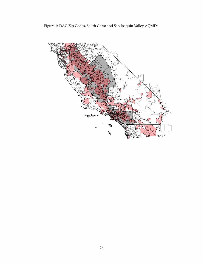
Figure 1: DAC Zip Codes, South Coast and San Joaquin Valley AQMDs

26

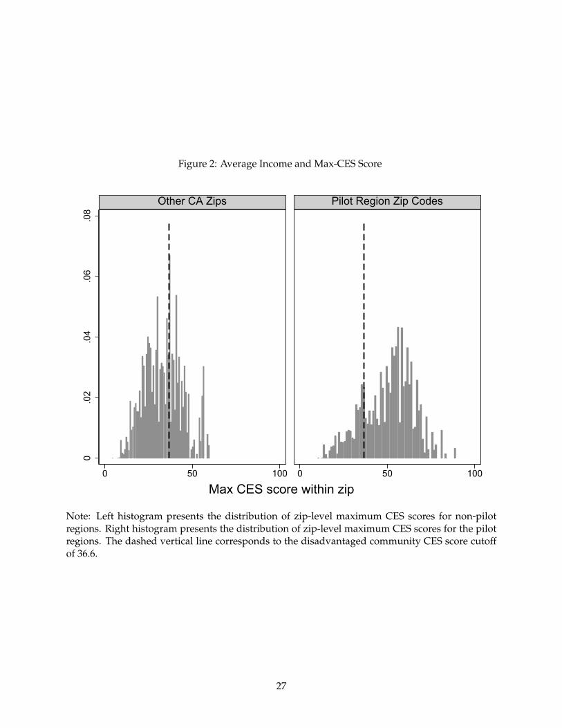
Figure 2: Average Income and Max-CES Score

0.0

2.0

4.0

6.0

8

0 50 100 0 50 100

Other CA Zips Pilot Region Zip Codes

Max CES score within zip

Note: Left histogram presents the distribution of zip-level maximum CES scores for non-pilotregions. Right histogram presents the distribution of zip-level maximum CES scores for the pilotregions. The dashed vertical line corresponds to the disadvantaged community CES score cutoffof 36.6.

27

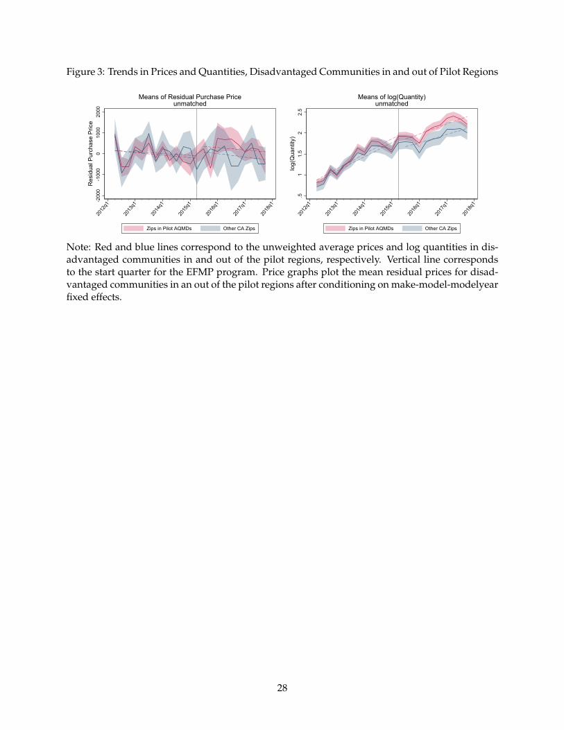
Figure 3: Trends in Prices and Quantities, Disadvantaged Communities in and out of Pilot Regions

-200

0-1

000

010

0020

00R

esid

ual P

urch

ase

Pric

e20

12q1

2013

q1

2014

q1

2015

q1

2016

q1

2017

q1

2018

q1

Zips in Pilot AQMDs Other CA Zips

Means of Residual Purchase Priceunmatched

.51

1.5

22.

5lo

g(Q

uant

ity)

2012

q1

2013

q1

2014

q1

2015

q1

2016

q1

2017

q1

2018

q1

Zips in Pilot AQMDs Other CA Zips

Means of log(Quantity)unmatched

Note: Red and blue lines correspond to the unweighted average prices and log quantities in dis-advantaged communities in and out of the pilot regions, respectively. Vertical line correspondsto the start quarter for the EFMP program. Price graphs plot the mean residual prices for disad-vantaged communities in an out of the pilot regions after conditioning on make-model-modelyearfixed effects.

28

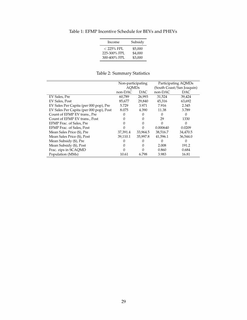
Table 1: EFMP Incentive Schedule for BEVs and PHEVs

Income Subsidy

< 225% FPL $5,000225-300% FPL $4,000300-400% FPL $3,000

Table 2: Summary Statistics

Non-participating Participating AQMDsAQMDs (South Coast/San Joaquin)

non-DAC DAC non-DAC DACEV Sales, Pre 60,789 26,993 31,524 39,424EV Sales, Post 85,677 29,840 45,316 63,692EV Sales Per Capita (per 000 pop), Pre 5.729 3.971 7.916 2.345EV Sales Per Capita (per 000 pop), Post 8.075 4.390 11.38 3.789Count of EFMP EV trans., Pre 0 0 0 0Count of EFMP EV trans., Post 0 0 29 1330EFMP Frac. of Sales, Pre 0 0 0 0EFMP Frac. of Sales, Post 0 0 0.000640 0.0209Mean Sales Price ($), Pre 37,391.4 33,964.5 38,516.7 34,470.5Mean Sales Price ($), Post 39,110.1 35,997.8 41,596.1 36,544.0Mean Subsidy ($), Pre 0 0 0 0Mean Subsidy ($), Post 0 0 2.008 191.2Frac. zips in SCAQMD 0 0 0.860 0.684Population (MMs) 10.61 6.798 3.983 16.81

29

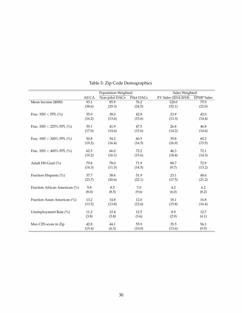
Table 3: Zip Code Demographics

Population Weighted Sales WeightedAll CA Non-pilot DACs Pilot DACs EV Sales (2014-2018) EFMP Sales

Mean Income ($000) 93.1 85.9 76.2 128.0 75.9(38.6) (29.3) (24.5) (52.1) (22.0)

Frac. HH < FPL (%) 35.0 38.0 42.8 23.9 42.0(16.2) (13.6) (15.6) (13.3) (14.4)

Frac. HH < 225% FPL (%) 39.1 41.9 47.5 26.8 46.8(17.0) (14.6) (15.6) (14.2) (14.6)

Frac. HH < 300% FPL (%) 50.8 54.2 60.5 35.8 60.2(19.2) (16.4) (16.5) (16.9) (15.5)

Frac. HH < 400% FPL (%) 62.5 66.0 72.2 46.3 72.1(19.2) (16.1) (15.6) (18.4) (14.3)

Adult HS Grad (%) 79.8 78.0 71.9 88.7 72.9(14.3) (11.5) (14.5) (9.7) (13.2)

Fraction Hispanic (%) 37.7 38.6 51.9 23.1 48.6(23.7) (20.6) (22.1) (17.5) (21.2)

Fraction African American (%) 5.8 8.5 7.0 4.2 6.2(8.0) (8.5) (9.6) (6.0) (8.2)

Fraction Asian American (%) 13.2 14.8 12.0 18.1 16.8(13.5) (13.8) (12.6) (15.8) (16.4)

Unemployment Rate (%) 11.2 12.4 12.5 8.9 12.7(3.8) (3.8) (3.6) (2.9) (4.1)

Max CES score in Zip 42.8 44.1 55.9 35.5 56.1(15.4) (6.3) (10.0) (13.6) (9.5)

30

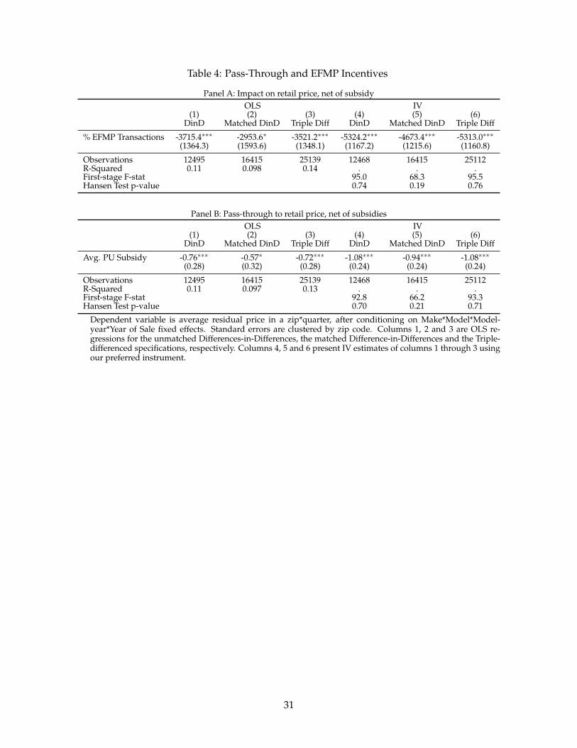
Table 4: Pass-Through and EFMP Incentives

Panel A: Impact on retail price, net of subsidyOLS IV

(1) (2) (3) (4) (5) (6)DinD Matched DinD Triple Diff DinD Matched DinD Triple Diff

% EFMP Transactions -3715.4∗∗∗ -2953.6∗ -3521.2∗∗∗ -5324.2∗∗∗ -4673.4∗∗∗ -5313.0∗∗∗(1364.3) (1593.6) (1348.1) (1167.2) (1215.6) (1160.8)

Observations 12495 16415 25139 12468 16415 25112R-Squared 0.11 0.098 0.14 . . .First-stage F-stat 95.0 68.3 95.5Hansen Test p-value 0.74 0.19 0.76

Panel B: Pass-through to retail price, net of subsidiesOLS IV

(1) (2) (3) (4) (5) (6)DinD Matched DinD Triple Diff DinD Matched DinD Triple Diff

Avg. PU Subsidy -0.76∗∗∗ -0.57∗ -0.72∗∗∗ -1.08∗∗∗ -0.94∗∗∗ -1.08∗∗∗(0.28) (0.32) (0.28) (0.24) (0.24) (0.24)

Observations 12495 16415 25139 12468 16415 25112R-Squared 0.11 0.097 0.13 . . .First-stage F-stat 92.8 66.2 93.3Hansen Test p-value 0.70 0.21 0.71

Dependent variable is average residual price in a zip*quarter, after conditioning on Make*Model*Model-year*Year of Sale fixed effects. Standard errors are clustered by zip code. Columns 1, 2 and 3 are OLS re-gressions for the unmatched Differences-in-Differences, the matched Difference-in-Differences and the Triple-differenced specifications, respectively. Columns 4, 5 and 6 present IV estimates of columns 1 through 3 usingour preferred instrument.

31

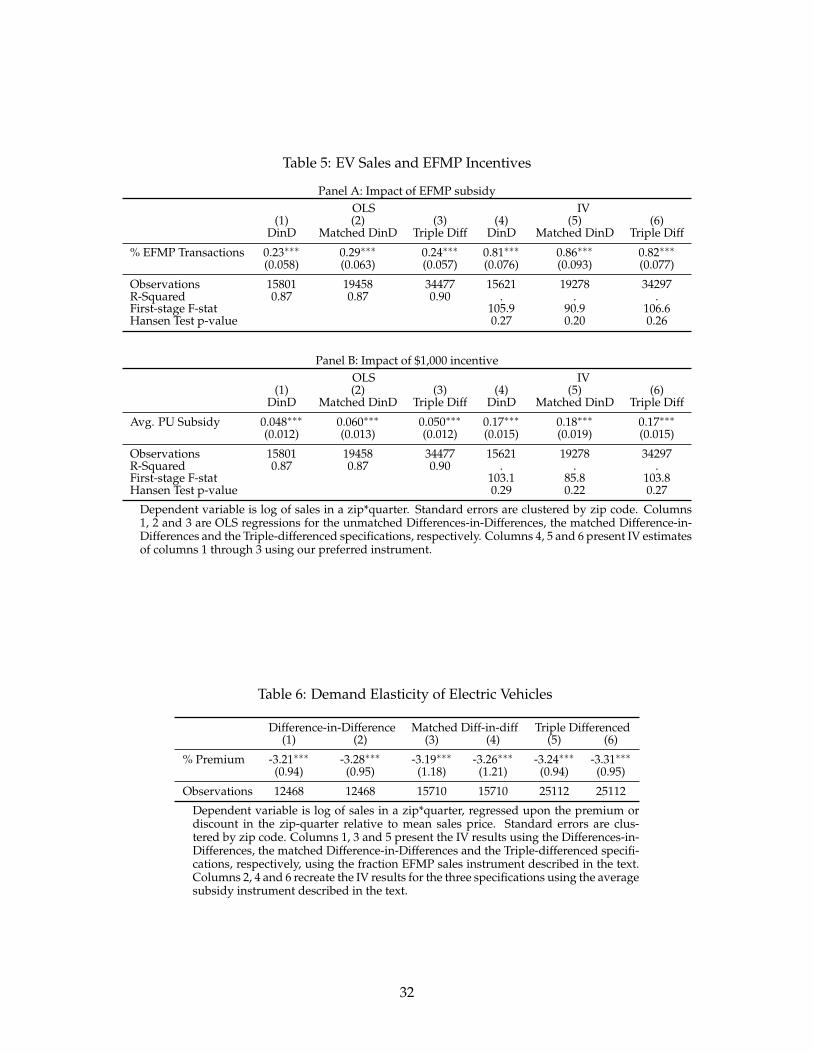
Table 5: EV Sales and EFMP Incentives

Panel A: Impact of EFMP subsidyOLS IV

(1) (2) (3) (4) (5) (6)DinD Matched DinD Triple Diff DinD Matched DinD Triple Diff

% EFMP Transactions 0.23∗∗∗ 0.29∗∗∗ 0.24∗∗∗ 0.81∗∗∗ 0.86∗∗∗ 0.82∗∗∗(0.058) (0.063) (0.057) (0.076) (0.093) (0.077)

Observations 15801 19458 34477 15621 19278 34297R-Squared 0.87 0.87 0.90 . . .First-stage F-stat 105.9 90.9 106.6Hansen Test p-value 0.27 0.20 0.26

Panel B: Impact of $1,000 incentiveOLS IV

(1) (2) (3) (4) (5) (6)DinD Matched DinD Triple Diff DinD Matched DinD Triple Diff

Avg. PU Subsidy 0.048∗∗∗ 0.060∗∗∗ 0.050∗∗∗ 0.17∗∗∗ 0.18∗∗∗ 0.17∗∗∗(0.012) (0.013) (0.012) (0.015) (0.019) (0.015)

Observations 15801 19458 34477 15621 19278 34297R-Squared 0.87 0.87 0.90 . . .First-stage F-stat 103.1 85.8 103.8Hansen Test p-value 0.29 0.22 0.27

Dependent variable is log of sales in a zip*quarter. Standard errors are clustered by zip code. Columns1, 2 and 3 are OLS regressions for the unmatched Differences-in-Differences, the matched Difference-in-Differences and the Triple-differenced specifications, respectively. Columns 4, 5 and 6 present IV estimatesof columns 1 through 3 using our preferred instrument.

Table 6: Demand Elasticity of Electric Vehicles

Difference-in-Difference Matched Diff-in-diff Triple Differenced(1) (2) (3) (4) (5) (6)

% Premium -3.21∗∗∗ -3.28∗∗∗ -3.19∗∗∗ -3.26∗∗∗ -3.24∗∗∗ -3.31∗∗∗(0.94) (0.95) (1.18) (1.21) (0.94) (0.95)

Observations 12468 12468 15710 15710 25112 25112

Dependent variable is log of sales in a zip*quarter, regressed upon the premium ordiscount in the zip-quarter relative to mean sales price. Standard errors are clus-tered by zip code. Columns 1, 3 and 5 present the IV results using the Differences-in-Differences, the matched Difference-in-Differences and the Triple-differenced specifi-cations, respectively, using the fraction EFMP sales instrument described in the text.Columns 2, 4 and 6 recreate the IV results for the three specifications using the averagesubsidy instrument described in the text.

32

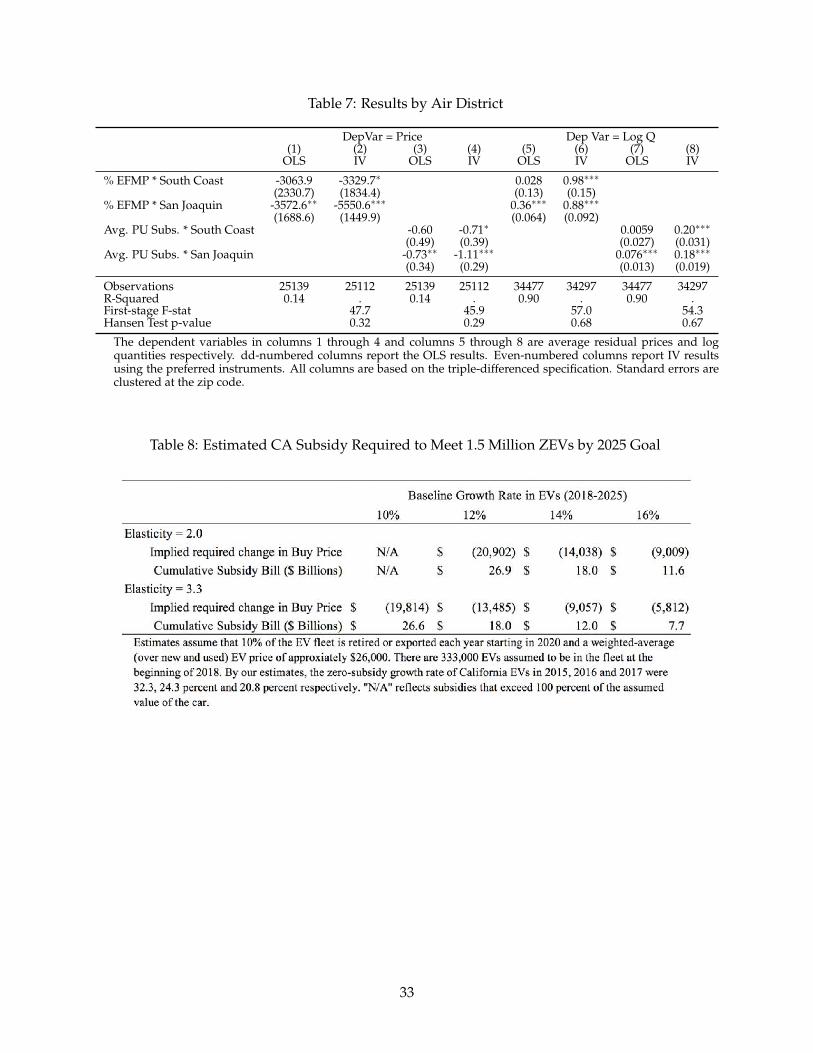
Table 7: Results by Air District

DepVar = Price Dep Var = Log Q(1) (2) (3) (4) (5) (6) (7) (8)

OLS IV OLS IV OLS IV OLS IV

% EFMP * South Coast -3063.9 -3329.7∗ 0.028 0.98∗∗∗(2330.7) (1834.4) (0.13) (0.15)

% EFMP * San Joaquin -3572.6∗∗ -5550.6∗∗∗ 0.36∗∗∗ 0.88∗∗∗(1688.6) (1449.9) (0.064) (0.092)

Avg. PU Subs. * South Coast -0.60 -0.71∗ 0.0059 0.20∗∗∗(0.49) (0.39) (0.027) (0.031)

Avg. PU Subs. * San Joaquin -0.73∗∗ -1.11∗∗∗ 0.076∗∗∗ 0.18∗∗∗(0.34) (0.29) (0.013) (0.019)

Observations 25139 25112 25139 25112 34477 34297 34477 34297R-Squared 0.14 . 0.14 . 0.90 . 0.90 .First-stage F-stat 47.7 45.9 57.0 54.3Hansen Test p-value 0.32 0.29 0.68 0.67

The dependent variables in columns 1 through 4 and columns 5 through 8 are average residual prices and logquantities respectively. dd-numbered columns report the OLS results. Even-numbered columns report IV resultsusing the preferred instruments. All columns are based on the triple-differenced specification. Standard errors areclustered at the zip code.

Table 8: Estimated CA Subsidy Required to Meet 1.5 Million ZEVs by 2025 Goal

33

A Appendix

A.1 Supplementary Figures and Tables

Figure A1: EFMP Eligibility Flowchart

EFMP/Plus-Up Flow Chart

June 22, 2017California Air Resources Board

10

Functional VehicleIncome Eligible

DAC?

EFMP

EFMP Plus-Up

PurchaseReplacement

Vehicle

Consumer Education & Protections

Scrap Old Vehicle

YesNoNot Eligible

Yes

No$4500 Max

$9500 Max

Consumer Applies

Source: https://www.arb.ca.gov/board/books/2017/062217/17-6-1pres.pdf

34

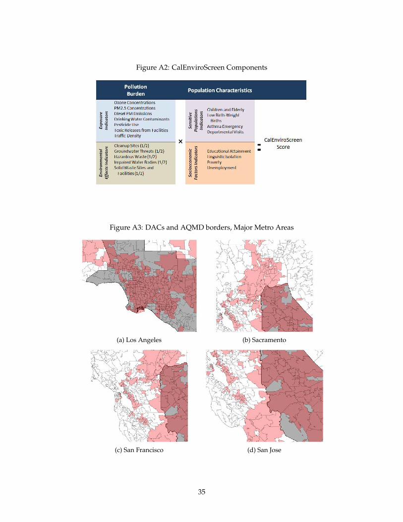
Figure A2: CalEnviroScreen Components

Figure A3: DACs and AQMD borders, Major Metro Areas

(a) Los Angeles (b) Sacramento

(c) San Francisco (d) San Jose

35

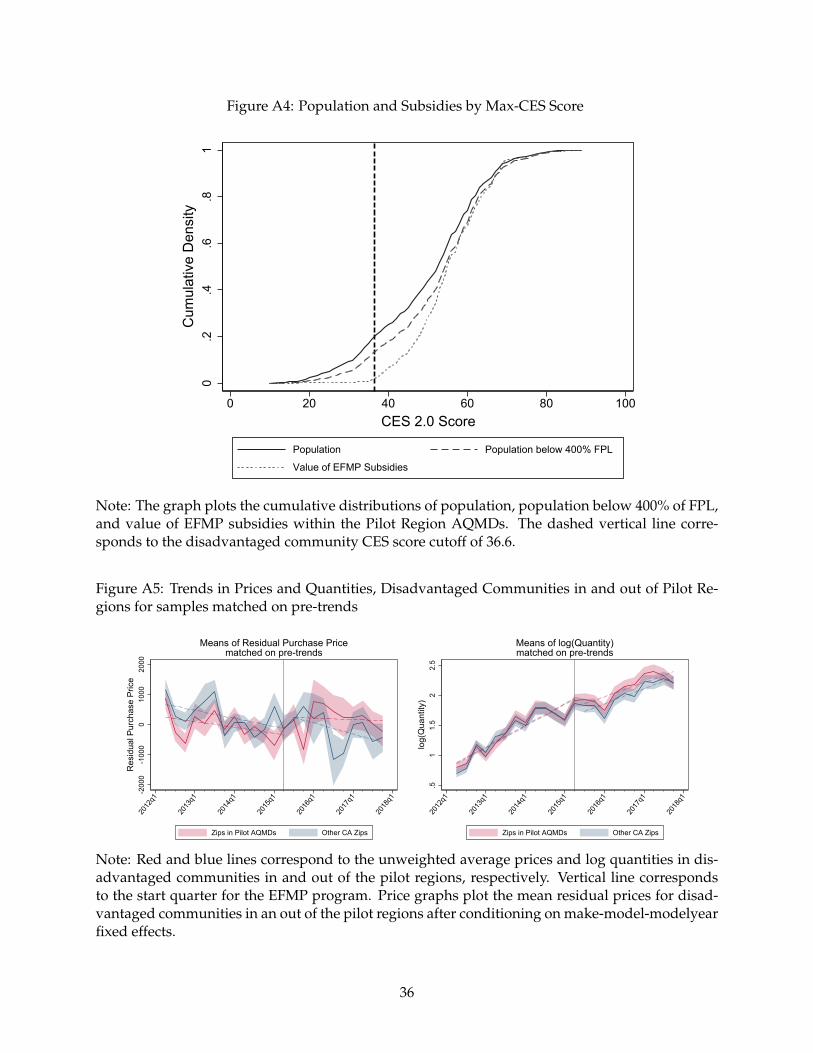
Figure A4: Population and Subsidies by Max-CES Score

0.2

.4.6

.81

Cum

ulat

ive

Den

sity

0 20 40 60 80 100CES 2.0 Score

Population Population below 400% FPL

Value of EFMP Subsidies

Note: The graph plots the cumulative distributions of population, population below 400% of FPL,and value of EFMP subsidies within the Pilot Region AQMDs. The dashed vertical line corre-sponds to the disadvantaged community CES score cutoff of 36.6.

Figure A5: Trends in Prices and Quantities, Disadvantaged Communities in and out of Pilot Re-gions for samples matched on pre-trends

-200

0-1

000

010

0020

00R

esid

ual P

urch

ase

Pric

e20

12q1

2013

q1

2014

q1

2015

q1

2016

q1

2017

q1

2018

q1

Zips in Pilot AQMDs Other CA Zips

Means of Residual Purchase Pricematched on pre-trends

.51

1.5

22.

5lo

g(Q

uant

ity)

2012

q1

2013

q1

2014

q1

2015

q1

2016

q1

2017

q1

2018

q1

Zips in Pilot AQMDs Other CA Zips

Means of log(Quantity)matched on pre-trends

Note: Red and blue lines correspond to the unweighted average prices and log quantities in dis-advantaged communities in and out of the pilot regions, respectively. Vertical line correspondsto the start quarter for the EFMP program. Price graphs plot the mean residual prices for disad-vantaged communities in an out of the pilot regions after conditioning on make-model-modelyearfixed effects.

36

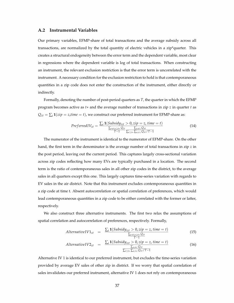
A.2 Instrumental Variables

Our primary variables, EFMP-share of total transactions and the average subsidy across all

transactions, are normalized by the total quantity of electric vehicles in a zip*quarter. This

creates a structural endogeneity between the error term and the dependent variable, most clear

in regressions where the dependent variable is log of total transactions. When constructing

an instrument, the relevant exclusion restriction is that the error term is uncorrelated with the

instrument. A necessary condition for the exclusion restriction to hold is that contemporaneous

quantities in a zip code does not enter the construction of the instrument, either directly or

indirectly.

Formally, denoting the number of post-period quarters as T, the quarter in which the EFMP

program becomes active as t∗ and the average number of transactions in zip z in quarter t as

Qzt = ∑i 1(zip = z,time = t), we construct our preferred instrument for EFMP-share as:

Pre f erredIVzt =∑i 1(Subsidyizt > 0, zip = z, time = t)

∑r 6=t,r≥t∗ QzrT−1

∑x 6=z Qxt∑r≥t∗ ∑x 6=z Qxr/T−1

(14)

The numerator of the instrument is identical to the numerator of EFMP-share. On the other

hand, the first term in the denominator is the average number of total transactions in zip z in

the post period, leaving out the current period. This captures largely cross-sectional variation

across zip codes reflecting how many EVs are typically purchased in a location. The second

term is the ratio of contemporaneous sales in all other zip codes in the district, to the average

sales in all quarters except this one. This largely captures time-series variation with regards to

EV sales in the air district. Note that this instrument excludes contemporaneous quantities in

a zip code at time t. Absent autocorrelation or spatial correlation of preferences, which would

lead contemporaneous quantities in a zip code to be either correlated with the former or latter,

respectively.

We also construct three alternative instruments. The first two relax the assumptions of

spatial correlation and autocorrelation of preferences, respectively. Formally,

AlternativeIV1zt =∑i 1(Subsidyizt > 0, zip = z, time = t)

∑r 6=t,r≥t∗ QzrT−1

(15)

AlternativeIV2zt =∑i 1(Subsidyizt > 0, zip = z, time = t)

∑x 6=z Qxt∑r≥t∗ ∑x 6=z Qxr/T−1

(16)

Alternative IV 1 is identical to our preferred instrument, but excludes the time-series variation

provided by average EV sales of other zip in district. If we worry that spatial correlation of

sales invalidates our preferred instrument, alternative IV 1 does not rely on contemporaneous

37

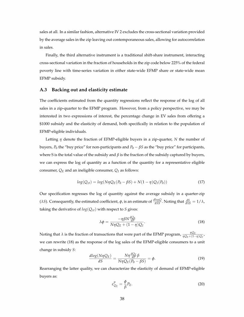
sales at all. In a similar fashion, alternative IV 2 excludes the cross-sectional variation provided

by the average sales in the zip leaving out contemporaneous sales, allowing for autocorrelation

in sales.

Finally, the third alternative instrument is a traditional shift-share instrument, interacting

cross-sectional variation in the fraction of households in the zip code below 225% of the federal

poverty line with time-series variation in either state-wide EFMP share or state-wide mean

EFMP subsidy.

A.3 Backing out and elasticity estimate

The coefficients estimated from the quantity regressions reflect the response of the log of all

sales in a zip-quarter to the EFMP program. However, from a policy perspective, we may be

interested in two expressions of interest, the percentage change in EV sales from offering a

$1000 subsidy and the elasticity of demand, both specifically in relation to the population of

EFMP-eligible individuals.

Letting η denote the fraction of EFMP-eligible buyers in a zip-quarter, N the number of

buyers, P0 the “buy price” for non-participants and P0− βS as the “buy price” for participants,

where S is the total value of the subsidy and β is the fraction of the subsidy captured by buyers,

we can express the log of quantity as a function of the quantity for a representative eligible

consumer, QE and an ineligible consumer, QI as follows:

log(Qzt) = log(NηQE(P0 − βS) + N(1− η)QI(P0)) (17)

Our specification regresses the log of quantity against the average subsidy in a quarter-zip

(λS). Consequently, the estimated coefficient, φ, is an estimate of dlogQdλS . Noting that dS

dλS = 1/λ,

taking the derivative of log(Qzt) with respect to S gives:

λφ =−ηβN dQE

dPNηQE + (1− η)QI

. (18)

Noting that λ is the fraction of transactions that were part of the EFMP program, ηQEηQE+(1−η)QI

,

we can rewrite (18) as the response of the log sales of the EFMP-eligible consumers to a unit

change in subsidy S:dlog(NηQE)

dS=

Nη dQEdP β

NηQE(P0 − βS)= φ. (19)

Rearranging the latter quality, we can characterize the elasticity of demand of EFMP-eligible

buyers as:

εPQE

=φ

βPE. (20)

38

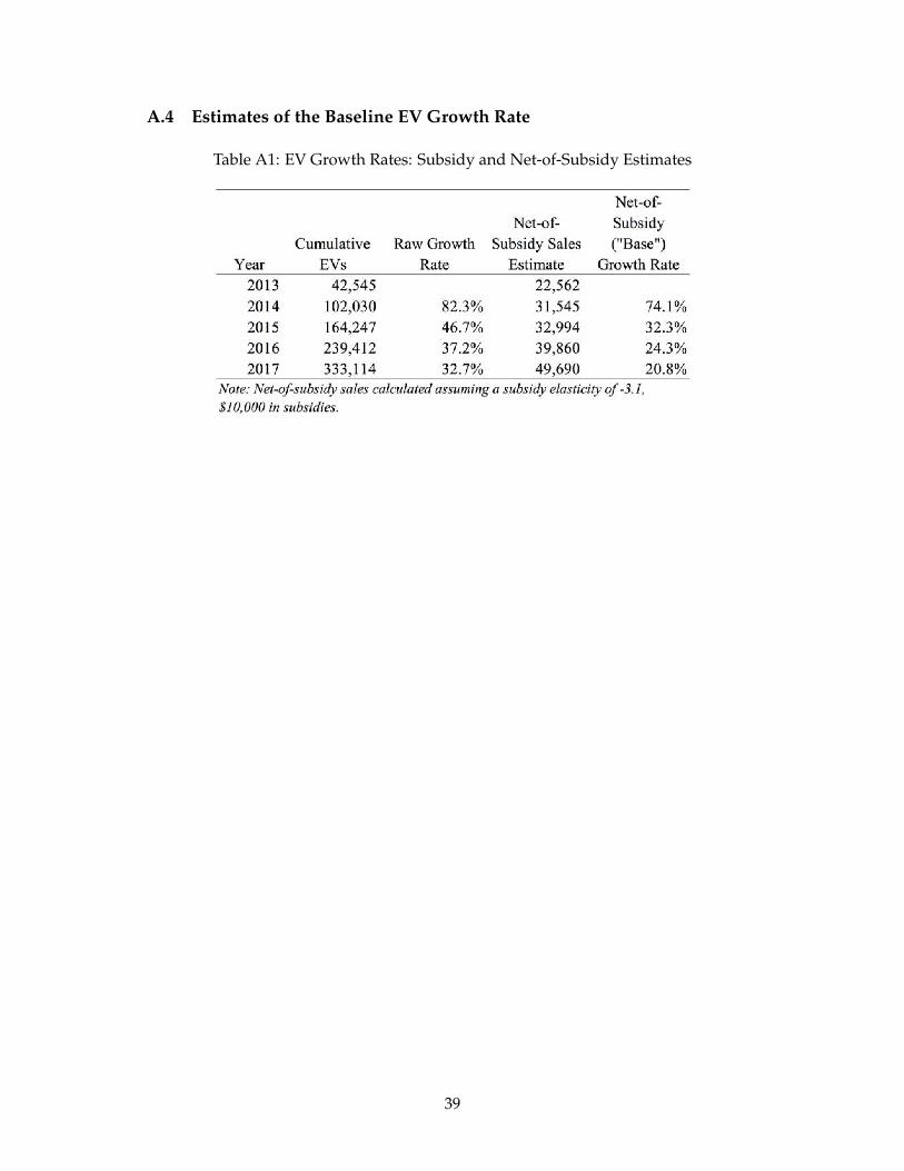
A.4 Estimates of the Baseline EV Growth Rate

Table A1: EV Growth Rates: Subsidy and Net-of-Subsidy Estimates

39