subject: date: ac no: engine rotors initiated by: change...

Subject: Damage Tolerance for High Energy TurbineEngine Rotors

Date: 1/8/01Initiated By:ANE-110

AC No: AC 33.14-1Change:

1. PURPOSE.

a. This advisory circular (AC) describes an acceptable means for showing compliancewith the requirements of § 33.14 of the Federal Aviation Regulations (Title 14, Code of FederalRegulations). Section 33.14 contains requirements applicable to the design and life managementof high energy rotating parts of aircraft gas turbine engines.

b. Like all advisory material, this AC is not, in itself, mandatory, and does not constitutea regulation. It is issued to describe an acceptable means, but not the only means, fordemonstrating compliance applicable to the design and life management of titanium alloy highenergy rotating parts of aircraft gas turbine engines. Terms such as "shall" and "must" are usedonly in the sense of ensuring applicability of this particular method of compliance when theacceptable method of compliance described in this document is used.

c. This AC does not change, create any additional, authorize changes in, or permitdeviations from the existing regulatory requirements.

2. RELATED READING MATERIAL.

a. FAA Advisory Circular: AC 33.2B, titled “Aircraft Engine Type CertificationHandbook”.

b. FAA Advisory Circular: AC 33.3, titled “Turbine and Compressor Rotor TypeCertification Substantiation Procedures”.

c. FAA Advisory Circular: AC 33.4, titled “Design Consideration Concerning the useof Titanium in Aircraft Turbine Engines”.

d. FAA Advisory Circular: AC 33.15, titled “Manufacturing Process of PremiumQuality Titanium Alloy Rotating Engine Components”.

AC 33.14-1 1/8/01

3. DEFINITIONS.

a. Component Event Rate. The number of events for a given titanium rotor componentstage for each flight cycle, calculated over the projected life of the component.

b. Critical Rotating Parts. Rotor structural parts (such as disks, spools, spacers, hubs,and shafts), the failure of which could result in a hazardous condition. In this context ahazardous condition should be interpreted as the conditions described in§ 33.75.

c. Damage Tolerance. This is an element of the life management process thatrecognizes the potential existence of component imperfections. The potential existence ofcomponent imperfections are the result of inherent material structure, material processing,component design, manufacturing or usage. Damage tolerance addresses this situation throughthe incorporation of fracture resistant design, fracture-mechanics, process control, ornondestructive inspection.

d. Default Probability of Detection (POD) Values. Values representing meanprobabilities of detecting anomalies of various types and sizes, under specified inspectionconditions consistent with good industry practice.

e. Design Target Risk (DTR) Value. This is the standard against which probabilisticassessment results (stated in terms of component event rates and engine level event rates, asdefined below) are compared.

f. Engine Event Rate. The cumulative number of events for each flight cycle, for allcritical titanium rotating parts in a given engine, calculated over the projected life of thosecomponents.

g. Event. A rotor structural part separation, failure, or burst with no regard to theconsequence.

h. Focused Inspection. A term used to describe inspections in which any necessaryspecialized processing instructions have been provided, and the inspector has been instructed topay attention to specific critical features.

i. Full Field Inspection. A term used to describe the general inspection of a componentwithout special attention to any specific features.

Par 3

1/8/01 AC 33.14-1

j. Hard-Alpha or High Interstitial Defect (HID). An interstitially stabilized alpha phaseregion of substantially higher hardness than the surrounding material. This comes from very highlocal nitrogen, oxygen, or carbon concentrations, which increase the beta transus and producethe high hardness, often brittle, alpha phase; also commonly called a Type I defect, low densityinclusion (LDI), or a hard-alpha; often associated with voids and cracks.

k. Hard Time Inspection Interval. The number of flight cycles since new or the mostrecent inspection, after which a rotor part must be made available and receive the inspectionspecified in the Airworthiness Limitations Section of the Instructions for ContinuedAirworthiness.

l. Inspected Material. That portion of the total volume of a component that is actuallyinspected under the described conditions. Inspected material does not guarantee anomaly freematerial.

m. Inspection Opportunity. An occasion when an engine is disassembled to at least themodular level and the hardware in question is accessible for inspection, whether or not thehardware has been reduced to the piece part level.

n. Low Cycle Fatigue (LCF) Initiation. The process of progressive and permanentlocal structural deterioration occurring in a material subject to cyclic variations, in stress andstrain, of sufficient magnitude and number of repetitions. The process will culminate indetectable crack initiation typically within 105 cycles. For the purposes of this AC, a detectablecrack initiation is defined as 0.030 inches in length by 0.015 inches in depth.

o. Maintenance Exposure Interval. Distribution of shop visits (in-flight cycles) sincenew or last overhaul that an engine, module, or component is exposed to as a function of normalmaintenance activity.

p. Mean POD. The 50-percent confidence level POD versus anomaly size curve.

q. Module Available. An individual module removed from the engine.

r. Module. A combination of assemblies, subassemblies, and parts contained in onepackage, or arranged to be installed in one maintenance action.

Par 3

AC 33.14-1 1/8/01

s. Part Available. A part that can be inspected, as required by the AirworthinessLimitations Section of the Instructions for Continued Airworthiness, without any furtherdisassembly. Depending on the inspection requirements, some parts may require a fullydisassembled “piece part” condition, while other parts may be available for inspection while stillin the assembled module.

t. Probabilistic (Relative Risk) Assessment. A fracture-mechanics based simulationprocedure that uses statistical techniques to mathematically model and quantitatively combinethe influence of two or more variables to estimate a most likely outcome or range of outcomesfor a product. Since not all variables may be considered or may not be capable of beingaccurately quantified, the numerical predictions are used on a comparative basis to evaluatevarious options having the same level of inputs. Results from these analyses are typically usedfor design optimization to meet a predefined target, or to conduct parametric studies. This typeof procedure is distinctly different from an absolute risk analysis, which attempts to consider allsignificant variables, and is used to quantify, on an absolute basis, the predicted number of futureevents having safety and reliability ramifications.

u. POD. A quantitative statistical measure of detecting a particular type of anomalyover a range of sizes using a specific nondestructive inspection technique under specificconditions. Typically, the mean POD curve is used.

v. Safe-Life. A LCF based process where components are designed and substantiatedto have a specified service life, which is stated in operating cycles or operating hours, or both.Continued safe operation, up to the stated life limit is not contingent upon each unit of a givendesign receiving interim inspections. When a component reaches its published life limit, it isretired from service.

w. Soft Time Inspection Interval. The number of flight cycles since new or the mostrecent inspection, after which a rotor part in an available module must receive the inspectionspecified in the Airworthiness Limitations Section of the Instructions for ContinuedAirworthiness.

x. Stage. The rotor structure which supports, and is attached to a single aerodynamicblade row.

1/8/01 AC 33.14-1

4. BACKGROUND.

a. Service experience with gas turbine engines has demonstrated that material andmanufacturing anomalies do occur. These anomalies can potentially degrade the structuralintegrity of high energy rotors. Conventional rotor life management methodology (safe-lifemethod) is founded on the assumption of the existence of nominal material variations andmanufacturing conditions. Consequently, the methodology does not explicitly address theoccurrence of such anomalies, although some level of tolerance to anomalies is implicitly built-inusing design margins, factory and field inspections, etc.

b. Under nominal conditions, this safe-life methodology provides a structured processfor the design and life management of high energy rotors, which results in the assurance ofstructural integrity throughout the life of the rotor. Undetectable material processing andmanufacturing induced anomalies, therefore, represent a departure from the assumed nominalconditions. In 1990, to quantify the extent of such occurrences the FAA requested that theSociety of Automotive Engineers (SAE) reconvene the ad hoc committee on uncontainedevents. The statistics pertaining to uncontained rotor events are reported in the SAE committeereport Nos. AIR 1537, AIR 4003, and SP-1270. While no adverse trends were identified, thecommittee expressed concern that the projected 5-percent increase in airline passenger trafficeach year would lead to a noticeable increase in the number of aircraft accidents fromuncontained rotor events. Uncontained rotor events have the potential to cause catastrophicaircraft accidents.

c. As a result of the accident at Sioux City in 1989, the FAA requested the turbineengine manufacturers, through the Aerospace Industries Association (AIA), to review availabletechniques to determine if a damage tolerance approach could be introduced which, ifappropriately implemented, could reduce the occurrence of uncontained rotor events.

d. The industry working group concluded that the technology was now available toimplement additional enhancements to the conventional rotor life management process, whichwould explicitly address anomalous conditions. Furthermore, these enhancements could bestructured to enforce design and life management adaptations, which would enhance rotorintegrity under anomalous material or manufacturing conditions. The additional guidelinesregarding damage tolerance provided in this AC explicitly address these anomalous conditions.In addition, the damage tolerance approach will also implicitly enhance damage tolerance toother anomalous conditions related to design, manufacture, maintenance and operation.

Par 4 Page 5

AC 33.14-1 1/8/01

5. APPLICABILITY.

a. This material has been prepared to present a generic damage tolerance approachwhich can be readily integrated with the existing “safe-life” process for high energy rotors toproduce an enhanced life management process. However, the data included in this AC are onlyapplicable to titanium alloy rotor components.

b. This material is intended to be applicable to all “new design” critical titanium alloyrotor components on a “go forward basis.” It is not intended to apply retroactively to existinghardware.

c. The new generic damage tolerance approach does not replace existing safe-lifemethodology, but expands upon it.

d. In the context of damage tolerance, it is not intended to allow operation beyond thecomponent manual limit set using the existing safe-life approach.

e. Rotor failure modes for which full containment can be demonstrated are excludedfrom the procedures outlined in this document and need not be accounted for in the overall riskassessment.

/s/David A. DowneyAssistant Manager, Engine & Propeller DirectorateAircraft Certification Service

CONTENTS

Page No.

Section 1 Conventional (“Safe-Life”) Life Management Process S1-1

Section 2 Enhanced Life Management Process S2-1

Section 3 Damage Tolerance Implementation S3-1

- Approach

- Methodology

- Default Input - Anomaly Distributions

- Default Input - Nondestructive Evaluation (NDE) Probability ofDetection (POD)

- Design Target Risk (DTR)

Section 4 “Soft-Time Inspection” Rotor Life Management Approach S4-1

Section 5 References S5-1

APPENDICES

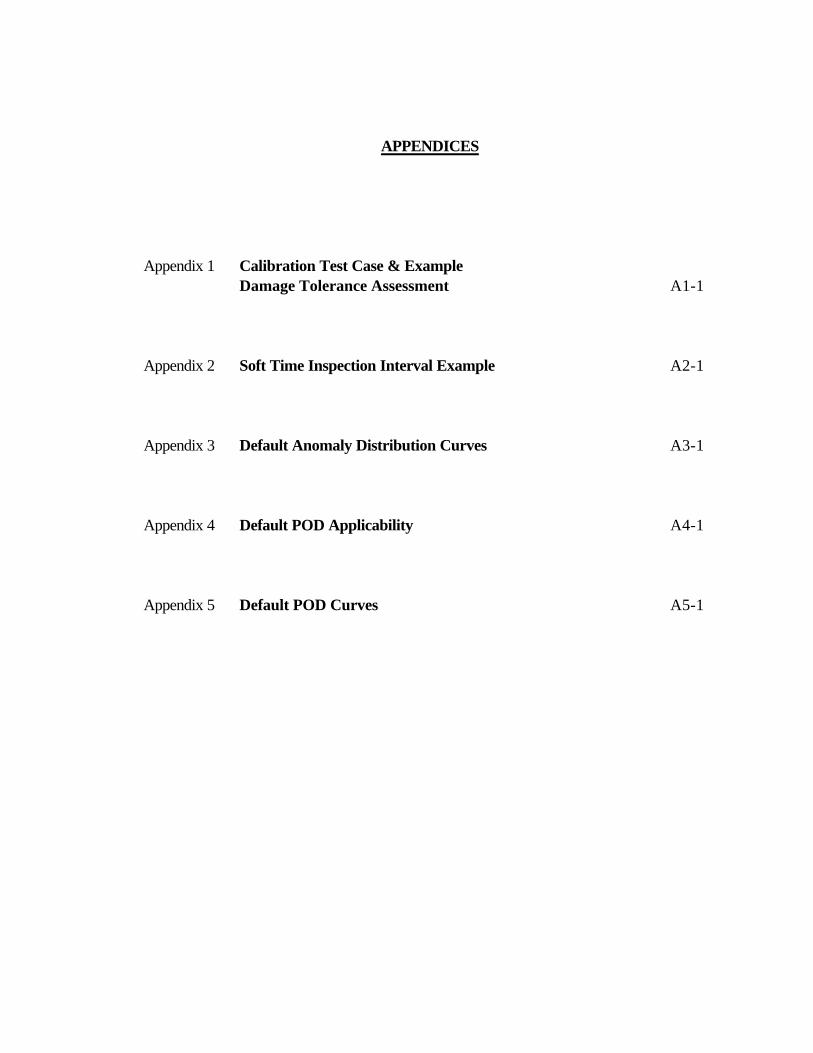
Appendix 1 Calibration Test Case & ExampleDamage Tolerance Assessment A1-1

Appendix 2 Soft Time Inspection Interval Example A2-1

Appendix 3 Default Anomaly Distribution Curves A3-1

Appendix 4 Default POD Applicability A4-1

Appendix 5 Default POD Curves A5-1

SECTION 1

CONVENTIONAL (“Safe-Life”) LIFE MANAGEMENT PROCESS

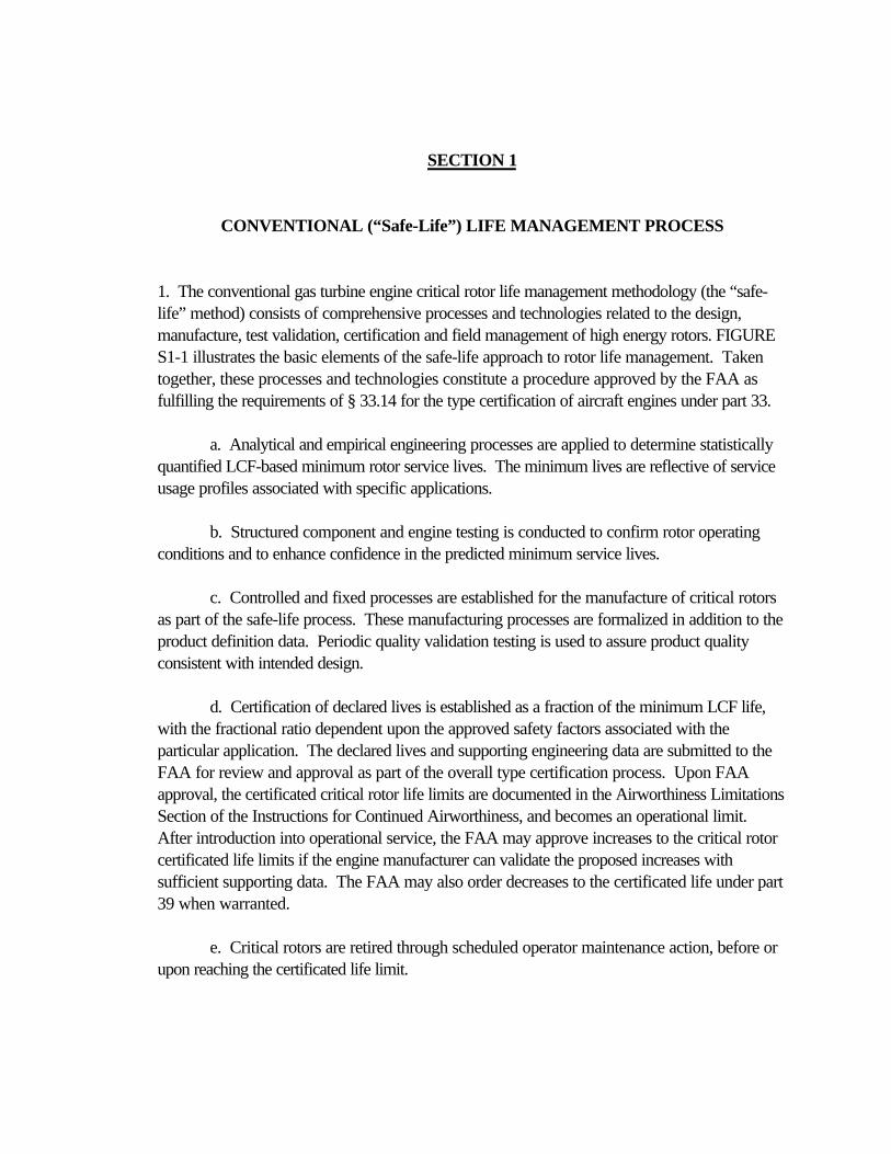
1. The conventional gas turbine engine critical rotor life management methodology (the “safe-life” method) consists of comprehensive processes and technologies related to the design,manufacture, test validation, certification and field management of high energy rotors. FIGURES1-1 illustrates the basic elements of the safe-life approach to rotor life management. Takentogether, these processes and technologies constitute a procedure approved by the FAA asfulfilling the requirements of § 33.14 for the type certification of aircraft engines under part 33.

a. Analytical and empirical engineering processes are applied to determine statisticallyquantified LCF-based minimum rotor service lives. The minimum lives are reflective of serviceusage profiles associated with specific applications.

b. Structured component and engine testing is conducted to confirm rotor operatingconditions and to enhance confidence in the predicted minimum service lives.

c. Controlled and fixed processes are established for the manufacture of critical rotorsas part of the safe-life process. These manufacturing processes are formalized in addition to theproduct definition data. Periodic quality validation testing is used to assure product qualityconsistent with intended design.

d. Certification of declared lives is established as a fraction of the minimum LCF life,with the fractional ratio dependent upon the approved safety factors associated with theparticular application. The declared lives and supporting engineering data are submitted to theFAA for review and approval as part of the overall type certification process. Upon FAAapproval, the certificated critical rotor life limits are documented in the Airworthiness LimitationsSection of the Instructions for Continued Airworthiness, and becomes an operational limit.After introduction into operational service, the FAA may approve increases to the critical rotorcertificated life limits if the engine manufacturer can validate the proposed increases withsufficient supporting data. The FAA may also order decreases to the certificated life under part39 when warranted.

e. Critical rotors are retired through scheduled operator maintenance action, before orupon reaching the certificated life limit.

f. Opportunity inspections, as part of the normal maintenance practices, are anotherelement of the conventional life management process. Even though the approval of certificatedlife limits is not contingent upon interim or even periodic inspections, most of the critical rotorsdo become available for inspection several times as part of normal engine maintenancepractices.

FIGURE S1-1: Typical Example Conventional Life Management Process

Performance Programs

Analysis Programs

Secondary Air FlowPrograms

Finite Element HeatTransfer Programs

Finite Element Stressand Vibration

Programs

Experimental Stress andVibration, Residual

Stress, Aeroelasticity

Materials Data: LaboratoryData, Static Rig Tests to

Understand Behavior

PerformanceFlight Profile Selection

Basic Design Data: Primary Air System, RPM, Temperature,

Pressure, Mass Flow

Internal, Secondary AirSystem Data: Flow

Stat ic Pressure Loads,Temperature

Transient MetalTemperature Estimation

Stress and VibrationAnalysis

Life Estimation: Routine,Special Circumstances

Service Life Certification

Aircraft & EngineRequirements

Vibratory StressMeasurements

Cyclic Rig Tests

Cyclic Engine Tests

Changes in Requirements

Flight Profile Monitoring

Design Changes

Manufacturing Changes

Inspection, NaturalArisings, Planned

Component and Engine,Time Expired Parts,

Special Circumstances

PerformanceMeasurements

Secondary Air systemFlow, PR, Temperature,

Measurements

Metal Temperature andInternal Air system

Measurements

PRODUCT ASSURANCEPROCEDURES APPLY

TO ALL ACTIVITIES

Methods andMaterials Data

LifeEstimation

Development andValidation Tests

Service Life andProduct Assurance

S1-3

g. The requirements for life estimation are represented by the elements in FIGURE S1-1. Life limits are to be specified for any engine rotor component where a failure of thatcomponent would result in a hazard to the aircraft. Within the cyclic life span, it is assumed thatcontinued safe operation of the specific rotor design, up to the stated life limit, is not contingentupon interim or periodic inspections. The key elements of life estimation include:

(1) Flight Cycle Definition: A flight cycle should be defined that considers themost severe and typical operation of the engine. The flight cycle provides the operationaldefinition so that the stress and thermal analyses can capture the transient and cyclical loading.The part lives are quoted in terms of this flight cycle. The flight cycle should include the variousflight segment such as start, idle, takeoff, climb, cruise, approach, landing, reverse andshutdown. The hold times at the various flight segments should correspond to the limitinginstallation variables (aircraft weight, climb rates, etc.). The corresponding rotor speeds,internal pressures, and temperatures during each flight segment should be adjusted to accountfor production tolerances and installation trim procedures, as well as engine deterioration thatcan be expected between heavy maintenance intervals. The range of ambient temperature andtakeoff altitude conditions encountered during the engines’ service life should also beconsidered.

(2) Thermal Analysis: The flight cycle along with the correspondingperformance data, act as boundary conditions for the thermal analysis. Temperature levels andthermal gradients should be determined throughout the flight cycle and should be calibrated andverified by engine rotor temperature data.

(3) Stress Analysis: Analytical and empirical engineering processes are appliedto determine the stress distribution for each structural part. The analyses evaluate the effects ofengine speed, pressure, metal temperature and thermal gradients at many discrete flight cycleconditions. From this, the component’s cyclic stress history is constructed. Stressconcentration effects due to geometric discontinuities such as dovetails, boltholes and contourchanges should be included.

(4) Life Prediction System: The life prediction system is based upon test dataobtained from cyclic testing of specimens and components fabricated from representativeproduction grade material to account for the manufacturing processes that affect LCF capability.Sufficient testing should be performed to evaluate the effects of elevated temperatures and holdtimes, as well as, interaction with other material failure mechanisms such as high cycle fatigue(HCF) and creep. Test data should be reduced statistically in order to express the results interms of minimum LCF capability (1/1000 or alternately -3 sigma) and the safe-life should bequoted to initiation of a fatigue crack. Appropriate prior service experience gained through asuccessful program of parts retirement or precautionary sampling inspections, or both, may beincluded to expand the database.

SECTION 2

ENHANCED LIFE MANAGEMENT PROCESS

1. History has shown that the safe-life philosophy has served the turbine engine industry andflying public well, and provides a solid base for further enhancement. Modifications to theconventional life management procedures should augment, not supplant, current approaches,which are based on the safe-life philosophy.

a. By adding a new element, damage tolerance, to the existing conventional lifemanagement process, the enhanced life management process has been defined to furtherminimize the occurrence of uncontained rotor failures and thus improve flight safety (seeFIGURE S2-1).

b. Use of the enhanced life management process depicted in FIGURE S2-1, will resultin damage tolerance assessments being conducted on critical titanium alloy rotor designs. Thesewill be fracture-mechanics based probabilistic risk assessments, the results of which will becompared to the agreed upon design target risk (DTR) values. Designs that satisfy these DTRvalues will be considered to comply with the requirements of § 33.14. The engine manufacturerwill have a variety of options available to achieve the DTR values. They include, but are notlimited to, component redesign, material changes, material process improvements, manufacturinginspection improvements, in-service inspections, and life limit reductions.

c. A general methodology for conducting the fracture-mechanics based probabilisticanalyses mentioned above is presented in Section 3 (Damage Tolerance Implementation).

S2-1

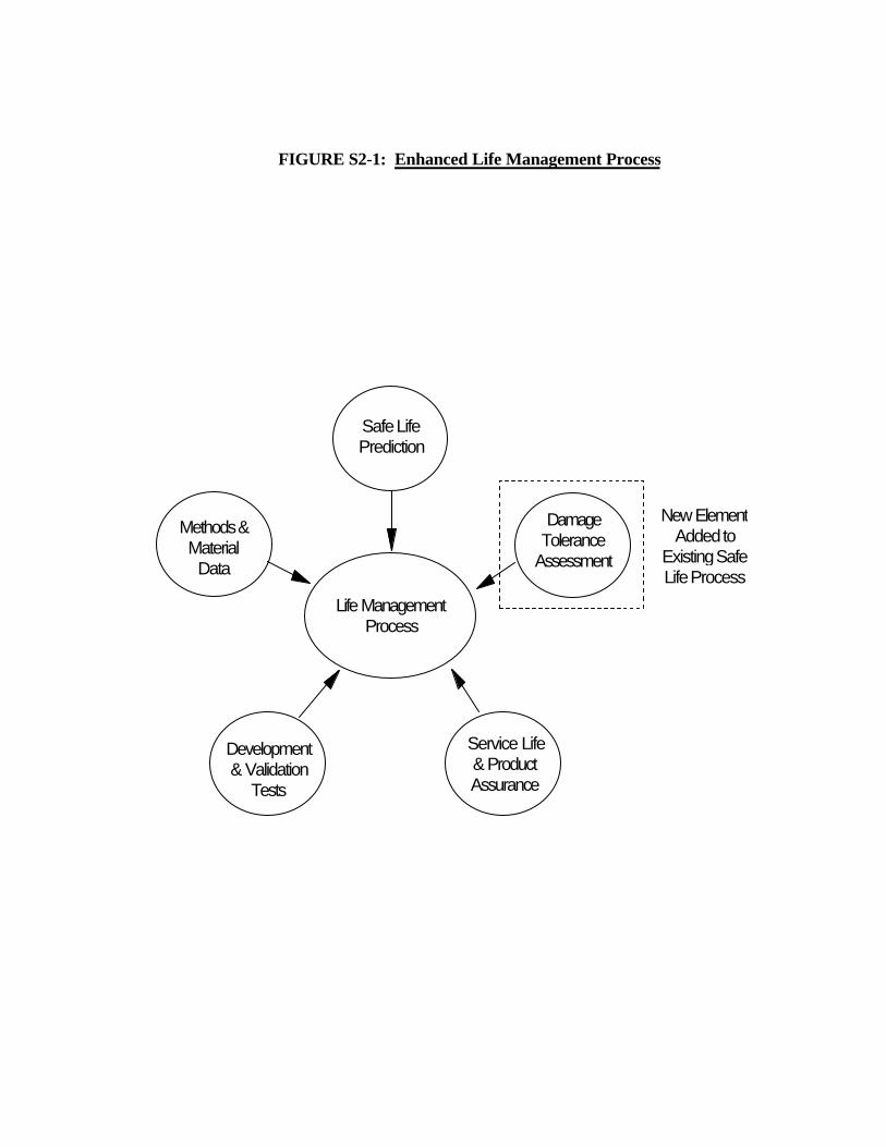
FIGURE S2-1: Enhanced Life Management Process

Life ManagementProcess

Development& Validation

Tests

Methods &MaterialData

Safe LifePrediction

Service Life& ProductAssurance

DamageTolerance

Assessment

New ElementAdded to

Existing SafeLife Process

SECTION 3

DAMAGE TOLERANCE IMPLEMENTATION

1. Approach

a. Fracture-mechanics based probabilistic (FMBP) assessments are a key feature ofthe enhanced life management process. The results of these assessments will provide the basisfor evaluating the relative damage tolerance capabilities of candidate engine designs, and willalso allow the engine manufacturer to balance the designs for both enhanced reliability andcustomer impact. The results will be compared against agreed upon DTR values (seeparagraph 5 of this Section).

b. The necessity for further risk reducing actions on the part of the engine manufacturerwill be based upon whether or not the design under consideration satisfies the desired DTRvalues at both the individual component level and the overall engine level. If the targets are met,then the design is considered to comply with § 33.14. The manufacturer may conductquantitative parametric studies to determine the influence of key variables such as inspectionmethods, inspection frequency, hardware geometry, hardware processing, material selectionand life limit reduction. The manufacturer may then make changes to the design or fieldmanagement of the part, or both, in order to achieve the agreed upon DTR values, as shown inFIGURE S3-1. This approach provides the individual engine manufacturer with the flexibility todevelop an optimal engine design solution consistent with customer requirements and companypolicies, procedures, and available resources. An example assessment utilizing thismethodology is described in paragraph 2 of this Section, and provided in Appendix 1 of thisAC.

c. FMBP assessments will usually be performed during the engine component detaildesign phase. Paragraph 2 of this Section defines an assessment methodology applicable tomaterial melt-related induced anomalies. It contains a standardized list of inputs for conductingFMBP assessments, and a process to refine a design to achieve the desired DTR values.

2. Methodology

a. Probabilistic risk assessments may be conducted using a variety of methods, such asMonte Carlo simulation or numerical integration techniques; the methodology

S3-1

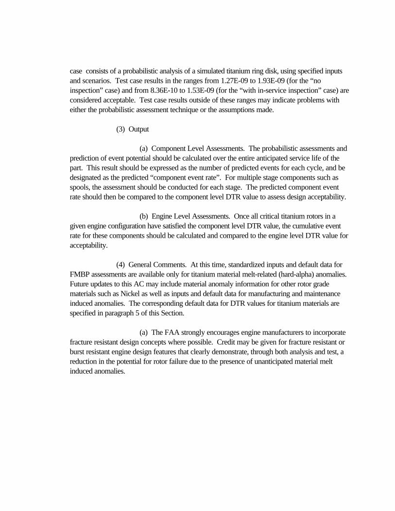
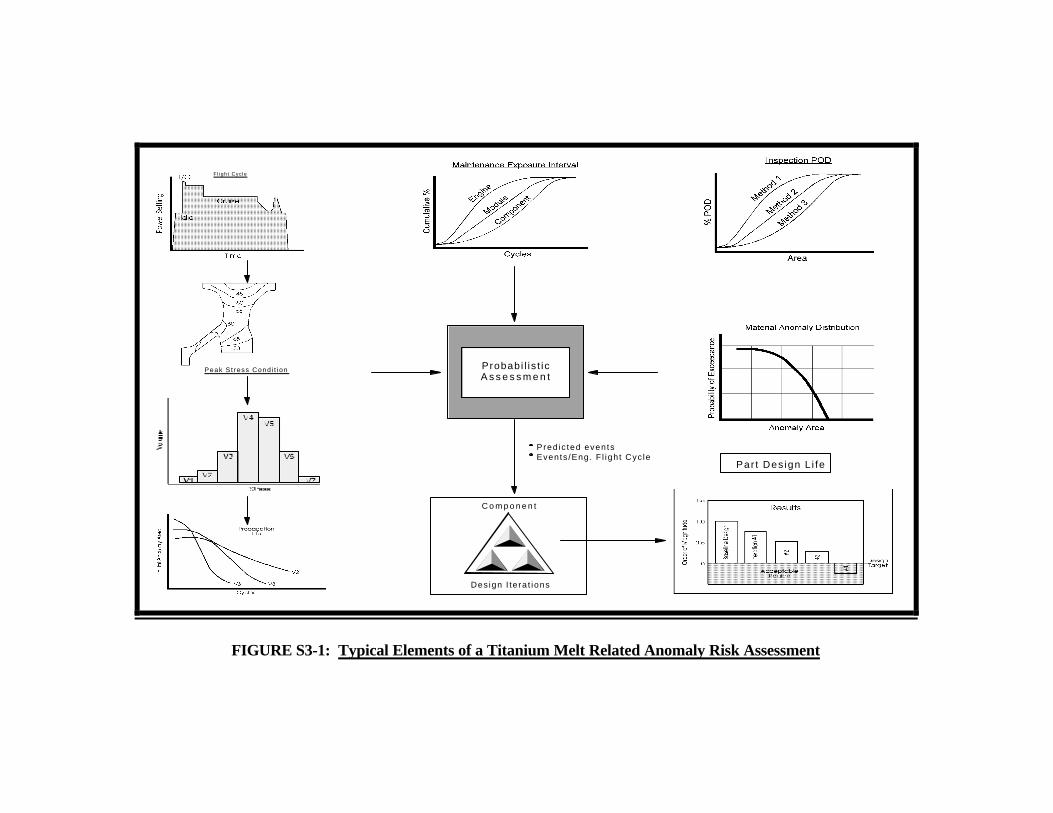
and assumptions used to determine the risk should be approved by the FAA. FIGURE S3-1conceptually depicts a melt-related anomaly probabilistic assessment. When performing anFMBP assessment, use of the standardized inputs and default data presented in this AC willachieve consistent FMBP assessment results across the industry.

b. A list of standardized inputs is provided below. Default input data is described inparagraphs 3 and 4 of this Section. Use of this default data in probabilistic assessments requiresno further demonstration of applicability or accuracy. However, where this data is used, theguidelines accompanying this data should be followed by the engine manufacturer to ensureapplicability. Use of input other than these default values may require additional validation toverify applicability, adequacy, and accuracy.

c. Probabilistic risk assessments should incorporate the following inputs as part of abasic analysis: component stress and volume, material properties, crack growth lives, anomalydistribution, design service life, inspection PODs, and maintenance exposure rate.

(1) Input. The following criteria are defined as basic input data.

(a) Anomaly Distribution. For melt-related (hard-alpha) assessments,use the default anomaly distributions outlined in paragraph 3 of this Section, or FAA approvedcompany-specific data. Company-specific data should be developed using the same processemployed to derive the default anomaly distributions. This process is described in a technicalpaper titled “Development of Anomaly Distributions for Aircraft Engine Titanium Disk Alloys”(see Section 5). Anomalies will be treated as sharp propagating cracks from the first stresscycle.

(b) POD. Default PODs and instructions on use of individual companyvalues are contained in paragraph 4 of this Section. Subsurface assessments should considerthe effects of ultrasonic inspection only. Surface assessments should likewise consider theeffects of fluorescent penetrant inspection (FPI) and eddy-current inspection (ECI).

(c) Maintenance Exposure Interval. For the purpose of assessinginspection benefits, exposure interval curves for the engine, module, or component in questionshould be modeled in the analysis.

(d) Stress. Variable influencing crack propagation life. Input shouldencompass the most limiting operational principal stresses. Subsurface

S3-2

assessments should incorporate the appropriate subsurface and near surface stress distribution.Surface assessments should incorporate the appropriate surface stress distributions, includingthe effects of stress concentration. Flight cycle(s) for design LCF certification, or actual usage(if known) should be used to establish the stress profile. The influence of major and minorcycles needs to be considered since the cyclic damage accumulation can be dramaticallydifferent for crack propagation as opposed to initiation. Note that the method described in thisAC has been calibrated against industry experience without consideration for the effect ofsurface enhancements such as shot peening on the predicted crack propagation lives. As aresult, it is inappropriate to include the beneficial effects of such enhancements on anycalculations at this time. This issue may be addressed in future revisions of this document.

(e) Volume. Affects the probability of having a defect in the material.Represents the volume of material at a specific level of stress. For subsurface assessments,represents the volume of material at various levels of subsurface stress. Surface assessmentsshould incorporate volume constituting a thin layer ("onion skin") around the surface of the part.Where a non-axisymmetric feature, such as a series of holes in a disk web has a localized stressconcentration, the decision on whether it makes a significant contribution to the probability ofburst must be based on the combination of mass of material at high stress and the size of theanomaly which would cause the part not to reach its safe declared life. While the methoddescribed in this AC assumes axisymmetric features, a non-axisymmetric feature can beincluded by reducing the cross-sectional area to ensure that the total volume when integratedaround the whole circumference is equal to the volume at high stress.

(f) Materials Data. Average cyclic crack growth rate properties of thebase material generated in an air environment, should be used as the default condition tocalculate anomaly propagation life.

(g) Propagation Life. Number of cycles for a given size anomaly togrow to a critical size. Based upon knowledge of part stress, temperature, geometry, stressgradient, anomaly orientation, and materials properties. Linear elastic fracture-mechanicsshould be used for the calculation of propagation life. Default conditions should assumeanomalies to be in the worst orientation to the stress field.

(2) Calibration

(a) Each engine manufacturer should calibrate its analytical predictiontools by conducting the industry test case detailed in Appendix 1. The test

S3-3

case consists of a probabilistic analysis of a simulated titanium ring disk, using specified inputsand scenarios. Test case results in the ranges from 1.27E-09 to 1.93E-09 (for the “noinspection” case) and from 8.36E-10 to 1.53E-09 (for the “with in-service inspection” case) areconsidered acceptable. Test case results outside of these ranges may indicate problems witheither the probabilistic assessment technique or the assumptions made.

(3) Output

(a) Component Level Assessments. The probabilistic assessments andprediction of event potential should be calculated over the entire anticipated service life of thepart. This result should be expressed as the number of predicted events for each cycle, and bedesignated as the predicted “component event rate”. For multiple stage components such asspools, the assessment should be conducted for each stage. The predicted component eventrate should then be compared to the component level DTR value to assess design acceptability.

(b) Engine Level Assessments. Once all critical titanium rotors in agiven engine configuration have satisfied the component level DTR value, the cumulative eventrate for these components should be calculated and compared to the engine level DTR value foracceptability.

(4) General Comments. At this time, standardized inputs and default data forFMBP assessments are available only for titanium material melt-related (hard-alpha) anomalies.Future updates to this AC may include material anomaly information for other rotor gradematerials such as Nickel as well as inputs and default data for manufacturing and maintenanceinduced anomalies. The corresponding default data for DTR values for titanium materials arespecified in paragraph 5 of this Section.

(a) The FAA strongly encourages engine manufacturers to incorporatefracture resistant design concepts where possible. Credit may be given for fracture resistant orburst resistant engine design features that clearly demonstrate, through both analysis and test, areduction in the potential for rotor failure due to the presence of unanticipated material meltinduced anomalies.

(b) Because the design of an aircraft turbine engine rotor is a lengthyprocess involving numerous iterations, each of which can substantially alter the initial calculatedDTR values, it is important that the DTR values be satisfied at the time of engine certification.Some FMBP assessments may also occur several years after the engine enters service becauseof such influences as design changes associated with in-service problems or changes in theanalytical results due to evolving predictive capability. It is important to state here that the DTRvalues should be satisfied at both the individual component and overall engine levels throughoutthe life of the hardware.

C o m p o n e n t

Des ign I te ra t ions

Probabi l is t icA s s e s s m e n t

Peak S t ress Cond i t i on

Par t Des ign L i fe

Pred ic ted even tsEvents /Eng. F l igh t Cyc le

F l igh t Cyc le

FIGURE S3-1: Typical Elements of a Titanium Melt Related Anomaly Risk Assessment

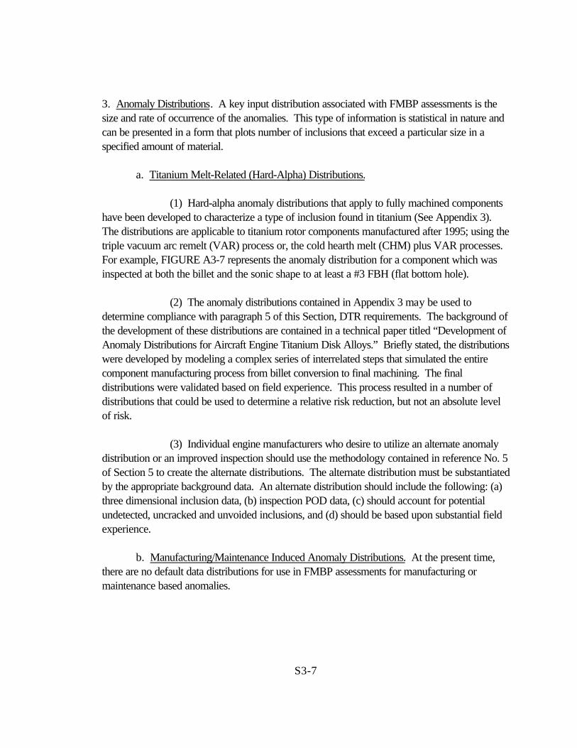
3. Anomaly Distributions. A key input distribution associated with FMBP assessments is thesize and rate of occurrence of the anomalies. This type of information is statistical in nature andcan be presented in a form that plots number of inclusions that exceed a particular size in aspecified amount of material.

a. Titanium Melt-Related (Hard-Alpha) Distributions.

(1) Hard-alpha anomaly distributions that apply to fully machined componentshave been developed to characterize a type of inclusion found in titanium (See Appendix 3).The distributions are applicable to titanium rotor components manufactured after 1995; using thetriple vacuum arc remelt (VAR) process or, the cold hearth melt (CHM) plus VAR processes.For example, FIGURE A3-7 represents the anomaly distribution for a component which wasinspected at both the billet and the sonic shape to at least a #3 FBH (flat bottom hole).

(2) The anomaly distributions contained in Appendix 3 may be used todetermine compliance with paragraph 5 of this Section, DTR requirements. The background ofthe development of these distributions are contained in a technical paper titled “Development ofAnomaly Distributions for Aircraft Engine Titanium Disk Alloys.” Briefly stated, the distributionswere developed by modeling a complex series of interrelated steps that simulated the entirecomponent manufacturing process from billet conversion to final machining. The finaldistributions were validated based on field experience. This process resulted in a number ofdistributions that could be used to determine a relative risk reduction, but not an absolute levelof risk.

(3) Individual engine manufacturers who desire to utilize an alternate anomalydistribution or an improved inspection should use the methodology contained in reference No. 5of Section 5 to create the alternate distributions. The alternate distribution must be substantiatedby the appropriate background data. An alternate distribution should include the following: (a)three dimensional inclusion data, (b) inspection POD data, (c) should account for potentialundetected, uncracked and unvoided inclusions, and (d) should be based upon substantial fieldexperience.

b. Manufacturing/Maintenance Induced Anomaly Distributions. At the present time,there are no default data distributions for use in FMBP assessments for manufacturing ormaintenance based anomalies.

S3-7

c. Rotor Grade Materials Other Than Titanium Alloy. At the present time, there are nodefault data distributions for use in FMBP assessments for rotors made of materials other thantitanium alloy.

4. Default Input - POD by Nondestructive Evaluation (NDE).

a. The capability of individual NDE processes, such as eddy-current, penetrant, orultrasonic inspection for the detection of local material anomalies (discontinuities or potentialanomalies), is a function of numerous parameters, including the size, shape, orientation, location,and chemical or metallurgical character of the anomaly. In addition, the following fourparameters should be considered when assessing the capabilities of an NDE process:

(1) The material being inspected (such as its composition, grain size,conductivity, surface texture, etc.).

(2) The inspection materials or instrumentation (such as the specific penetrantand developer, the inspection frequency, instrument bandwidth and linearity, etc.).

(3) The inspection parameters (such as scan index).

(4) The inspector (such as visual acuity, attention span, training, etc.).

b. The “default” POD data supplied with this AC are characteristic of inspectioncapability that has been measured under typical, well controlled conditions. These default PODvalues are provided primarily to facilitate selection of nondestructive inspection techniques thatare best suited to support attainment of damage tolerant inspections. It must be recognized that,although properly applied inspections should result in capability similar to these default values,they are strictly applicable only under the conditions under which they were acquired (seeAppendix 4). If exacting use is to be made of these data, skilled professional judgment as totheir applicability will be necessary. POD curves are described in Appendix 5, FIGURES A5-1-A5-5, as listed below:

(1) Appendix 5, FIGURE A5-1. Mean POD for Fluorescent PenetrantInspection of Finish-Machined Surfaces.

S3-8

(2) Appendix 5, FIGURE A5-2. Mean POD for #1 FBH UltrasonicInspection of Field Components.



(5) Appendix 5, FIGURE A5-5. Mean POD for Eddy-Current Inspection ofFinish Machined Surfaces.

NOTE: Refer to Appendix 1 for an example of the use of this data, and Appendix 4 for theNDE Applicability of these POD curves.

5. Design Target Risk (DTR).

a. The DTR is an agreed upon benchmark risk level selected to enhance the overallsafety of high energy titanium rotating components. Since no machine or device is 100-percentreliable, it is inappropriate to require a level that is technologically unachievable. Nevertheless,the goal is to achieve a significant and distinct improvement over and above current rotordesigns.

b. Representative “Component level DTRs” and an “engine level DTR” for titaniumhard-alpha anomalies have been established based on improvements of the data presented inthe SAE report. These DTRs represent consensus values, developed from assessments onrepresentative component designs using the methodology and inputs (described in paragraphs1-4 of Section 3). The “component level DTR” corresponds to the maximum allowablepredicted component event rate. The “engine level DTR” corresponds to the maximumallowable (cumulative) component event rate for all critical titanium rotating parts in a givenengine.

c. Designs must satisfy the component level DTR and the engine level DTR to beconsidered acceptable.

(1) Application. Default DTR values have been established for melt related(hard-alpha) anomalies. Calculated event rates should be assessed against the

appropriate DTR values. For multiple stage components, such as spools, each individual stagemust satisfy the component level DTR value.

(2) Default DTR values for titanium alloys:

(a) Melt related (hard-alpha) anomalies:

component level DTR: 1 x 10-9 events/flight cycle engine level DTR: 5 x 10-9 events/flight cycle

(b) Manufacturing or Maintenance Induced Surface Anomalies: At thepresent time, there are no default DTR values for manufacturing or maintenance related surfaceanomalies.

(3) Default DTR Values for Other Than Titanium Alloy: At the present time,there are no default DTR values for other than titanium alloys.

SECTION 4

“SOFT TIME INSPECTION” ROTOR LIFE MANAGEMENT

1. Approach. The overall life management process encompasses a wide spectrum of design,manufacture, and product support issues. This section addresses only one facet of that overallprocess, namely the assurance of structural integrity using inspection techniques and intervalsderived from a damage tolerance (fracture-mechanic based) assessment. The inspectionphilosophy is solely intended to protect against anomalous conditions. It is not intended to allowoperation beyond the safe-life limit specified in the Airworthiness Limitations Section of theInstructions for Continued Airworthiness.

a. In instances where probabilistic assessment indicates risk levels greater than thedesired target, many strategies can be utilized to reduce the predicted risk to the appropriatelevel. However, only the in-service inspection option is addressed here.

b. The industry data on uncontained fracture experience summarized in SAE reportsAIR 1537 (1959 through 1975), AIR 4003 (1976 through 1983), and SP1270 (1984 through1989) was used to guide the development of the inspection philosophy. These reports indicatethat the maintenance induced uncontained failure rates were comparable to the failure rates foranomalous conditions (material and manufacture). This data suggests that additional inspectionrequirements, if not properly integrated into the normal maintenance scheduled for the engine,would have no net benefit to the uncontained failure rates.

c. The inspection philosophy presented here evolved from the desire to haveinspections easily integrated into the operation of the engine yet achieve measurable reduction inthe uncontained failure rates. The inspection philosophy advocates the use of opportunityinspections rather than forced inspections at ‘not to exceed’ intervals. These opportunityinspections occur due to the ‘on condition’ maintenance practices used by operators today.Although the opportunity inspections occur at random intervals, they can be treated statisticallyand used effectively to lower the calculated risk of an uncontained event.

d. Opportunity inspection refers to those instances when the hardware in question isavailable in a form such that the specified inspection can be performed. This condition

S4-1

is generally viewed as being reduced to the piece part; however; opportunity inspections can beperformed on assembled modules. For example, an ECI of a disk bore may be specified on anassembled module whenever the module is available. This inspection is an opportunityinspection based upon module availability rather than piece part availability.

e. Whenever possible, the designs should use opportunity inspections to meet the DTRlevels. However, in some instances, the probabilistic analysis may indicate unacceptable risklevel when using just opportunity inspections and some additional action may be required tomeet the DTR. One of the many options to mitigate this risk is to force inspection opportunitiesby specifying disassembly of modules or engines when a cyclic life interval has been exceeded.There are many options on how to implement the forced disassembly. The options range frommandatory engine removal and subsequent teardown at not to exceed cyclic limits (“hard-time”limits) to mandatory module teardown when the naturally occurring module availability exceedsthe specified cyclic life inspection interval of one of the parts contained within that module(“soft-time” limits). This AC only advocates the use of the soft-time inspection option whenforced disassembly of modules is required to meet the DTR levels.

f. The soft-time inspection philosophy retains the “on-condition” maintenance practiceand minimizes the impact of additional module disassembly. The inspection requirement comesinto effect only after the engine has been removed from the aircraft for a reason other than theinspection itself, and is in a sufficient state of disassembly to afford access to the modulecontaining the component in question. An available module containing a part with cycles sincelast inspection (CSLI) in excess of the soft-time interval will be required to be disassembled to acondition that allows inspection by the procedure specified by the engine manufacturer. Therisk associated with parts that become available for inspection before the soft-time interval mustbe evaluated by the engine manufacturer to determine if the CSLI can be reset.

g. The maintenance impact of the soft-time intervals should be considered during thedesign phase. The probabilistic analysis summarized in Section 3 should be used along with theanticipated engine removal rate and the module and piece part availability to develop designsthat achieve the design target, but also result in acceptable soft-time intervals and procedures,should such action be required.

h. When invoked, the soft-time inspection approach establishes interval limits beyondwhich rotor components must be inspected when the rotors are available in modular form. Thesoft-time inspection requirement is not intended to impact or modify

S4-2

current practice of forced inspection programs to address safety of flight concerns that arise inthe course of engine operation and maturation. These safety of flight concerns would continueto be addressed through aggressive inspection programs which are mandated throughAirworthiness Directives (ADs).

i. It is important to recognize that the inspection assumptions made in the probabilisticrisk assessment must be communicated and implemented accurately to the field by using theAirworthiness Limitations Section of the Instructions for Continued Airworthiness, and bevalidated by the review of engine removal rates and module and piece part availability data. Forexample, the Airworthiness Limitations Section must call out an immersion ultrasonic inspectionif that was an assumption in setting the original soft-time interval. Similarly, the amount ofinspected material should correspond to the analysis assumptions. Likewise, if the fieldexperience suggests that the opportunity inspection intervals are in excess of the assumed ratesin the probabilistic risk assessment, then appropriate corrective action, such as a modifiedinspection plan, is required.

j. The soft-time inspection interval and reference to the corresponding inspectionprocedures will be specified in the Airworthiness Limitations Section of the Instructions forContinued Airworthiness. This information is to be provided for all rotor parts with specifiedretirement life limits that require any inspection plans beyond opportunity inspections to meet theDTR levels. The required inspection information should also be included in the individualAirworthiness Limitations Section of the Instructions for Continued Airworthiness with the otherrotor inspection requirements. The manufacturer will also provide necessary information tofocus the prescribed inspections to those areas of highest relative risk.

2. Inspection Scenarios.

a. The following scenarios clarify the action that would be taken at a maintenanceinspection opportunity. Note that the inspection plans may vary for each part, depending on theoutcome of the probabilistic assessments.

(1) Maintenance Opportunity - Hardware Available For OpportunityInspection: Hardware available in the condition to perform the specified opportunity inspectionmust be inspected by the procedures specified in the Airworthiness Limitations Section of theInstructions for Continued Airworthiness. This would be a mandatory inspection.

S4-5

(2) Maintenance Opportunity - Module Below Soft Time Interval: Hardwareaccessible in the assembled or partially disassembled module may be nondestructively inspectedby the procedures specified in the Airworthiness Limitations Section of the Instructions forContinued Airworthiness. The CSLI may be reset to zero, provided the engine manufacturerhas assessed the risk impact associated with this action. This would be a discretionaryinspection.

(3) Maintenance Opportunity - Module Above Soft Time Interval: Hardwarelisted in Airworthiness Limitations Section of the Instructions for Continued Airworthiness mustbe made available for nondestructive inspection, using the procedures that are specified. Thisinspection must be performed whenever the module is available and the CSLI for any containedhardware that exceeds the inspection cycle limit. This would be a mandatory inspection.

S4-6

SECTION 5

REFERENCES

1. SAE/FAA Committee On Uncontained Turbine Engine Rotor Events, Report No. AIR1537, Data Period 1962-1975.

2. SAE/FAA Committee On Uncontained Turbine Engine Rotor Events, Report No. AIR4003, Data Period 1976-1983.

3. SAE/FAA Committee On Uncontained Turbine Engine Rotor Events, Report No. SP-1270, Data Period 1984-1989.

4. FAA Advisory Circular 33.15, “Manufacturing Process of Premium Quality TitaniumAlloy Rotating Engine Components,” September 22, 1998.

5. “Development of Anomaly Distributions for Aircraft Engine Titanium Disk Alloys” -Technical paper was presented by the AIA Rotor Integrity Sub-Committee at the AmericanInstitute of Aeronautics and Astronautics (AIAA) Conference in April 1997.

APPENDIX 1

CALIBRATION TEST CASE

1. This Appendix provides a self contained package for calibration of a probabilistic riskassessment methodology. The package includes all required input data for the test case,analysis guidelines, and a test case analysis section that permits manufacturers to estimate thelevel of acceptability of their risk calculations and gain insights on intermediate results.

2. Test Case Input data

a. Anomaly distribution curve. The anomaly distributions are provided in Appendix 3.For this test case we will use the anomaly distribution presented in FIGURE A3-7 of Appendix3 titled “Post 1995 Triple Melt Hard-Alpha Distribution with #3 FBH billet inspection and #3FBH forging inspection”. Billet and forging manufacturing inspections are fully accounted for inthis curve. No additional modifications are necessary.

(1) It is assumed that anomalies are spherically shaped and uniformlydistributed throughout the part.

(2) The anomaly distribution should be linearly extrapolated when anomalysizes are required outside the range of data provided. The curve is shown in FIGUREA1-11.

b. POD. The POD curve used to determine the effect of an in-service inspection iscontained in Appendix 5. The default curve to be used is the mean POD for ultrasonicinspection of field components, with reject indications equal to or greater than those from a 3/64inch (1.19 mm) diameter FBH. For the test case, it is assumed that this curve applies to thewhole volume, including the near surface volume of the component.

c. Maintenance exposure interval. It should be assumed that 100-percent of the fleet isultrasonically inspected at 10,000 cycles, which represents 50-percent of the certified part life(20,000 cycles).

A1-1

d. Incubation. No anomaly incubation life should be assumed.

e. Stress. The limiting operational principal stress is the hoop stress.

f. Material Data. Two sets of material data are provided:

(1) Physical properties. Data required:

Density: 4,450 kg/m3 or 0.161 lb./in3

Young modulus: 120,000 MPa or 17.4E3 ksiPoisson's ratio: 0.361

(2) Crack Growth. Assume the following data represents both air and vacuumcrack propagation. Crack propagation rate:

da/dN = 9.25 E-13 (∆K)3.87 (da/dN in m/cycle and ∆ K in MPa√m)

- or -

da/dN = 5.248 E-11 (∆K)3.87 (da/dN in in/cycle and ∆ K in ksi√in )K threshold = 0.0 MPa√m or 0 ksi√inFracture toughness = 64.5 MPa√m or 58.7 ksi√inYield = 834 MPa or 121.0 ksiUTS = 910 MPa or 132.0 ksi

(a) The above data applies at the test case component temperature.

(b) Crack propagation data are for a stress ratio of zero, therefore, nostress ratio correction is required.

(c) These data were taken from MCIC-HB-01R, Damage TolerantDesign Handbook, A Compilation of Fracture and Crack Growth Data for High Stress Alloys,vol. 1, dated December 1983 (page 411.257, Figure 4.113.104). It represents generic Ti 6-4Paris fit data. These data are provided for example purposes only, and do not constitute arecommendation for analyzing actual components.

3. Test Case Analysis Guidelines

a. Analytical guidelines for the probabilistic assessments are provided with the intent tominimize the variations of the applicants results due to analytical assumptions.

The practice presented is based on a typical embedded anomaly probabilistic fracture-mechanics approach. The component is subdivided into zones, the relative risk or probability offracture (POF) is calculated for each zone, and results for each zone summed statistically toarrive at the total component POF or relative risk.

(1) This analytical approach can be broken down into five basic steps:

(a) Stress analysis.

(b) Zone definition and volume calculation.

(c) Crack growth model definition.

(d) Crack growth calculation.

(e) Zone and total part POF calculation.

(f) Paragraph 4 of this Appendix provides a systematic example for thecalibration test case.

b. General Analytical Guidelines:

(1) Stress Analysis. The level of mesh refinement of the part model is left up tothe individual applicant’s discretion. However, steps should be taken to ensure that the finalanswer does not change by a significant amount (5-percent on relative risk or POF) if a finermesh is chosen.

(2) Zone Definition. Zones are defined as regions of the component (typicallymade up of a number of finite elements) where life is approximately constant for a given initialcrack size. Grouping elements into zones based on stress intervals of 5

ksi (34.5 Mpa) is a suggested practice for initial zone definition. Further zone refinements maybe required for analytical convergence. FIGURE A1-1 provides a general description of thetypical types of zones.

FIGURE A1-1

surface

subsurfacea

subsurfacec

surf

ace

a

before break-out/transitionafter break-out/transition

surfacec

(3) Crack Growth Calculation. The crack growth life assumed for each zoneshould be based on the minimum life location in the zone. This conservative assumption mayrequire that regions of the component that make a significant contribution to the total part POFbe broken down into multiple zones. This subdivision process is carried out until convergenceof the risk calculation is reached.

NOTE: The effect of surface enhancement, such as shot-peen, is not considered in the testcase analysis. However, once the test case has been performed and the analysis processsuccessfully calibrated, the manufacturer may consider these effects when analyzing actualhardware.

(4) POF/Risk Calculation. The POF of the part is calculated by statisticallycombining the POF of each zone (surface and subsurface). The POF of each zone can becalculated in either of two ways:

(a) An integrated probabilistic method.

(b) A ‘’Monte - Carlo’’ method. The number of simulations requiredis related to the computed risk. The general rule is that the number of simulations should be atleast 2 orders of magnitude higher than the computed risk, for example, if risk is 1 failure in 104

parts, the number of samples required is 106. This ensures that about 100 “failed” parts areinvolved in the assessment.

c. Specific Guidelines for Fracture-Mechanics Modeling, Zone Definition, and VolumeCalculations:

(1) Subsurface Zones.

(a) Surface enhancements must not be modeled for the test case,however, they should be considered when analyzing actual components.

(b) The maximum principal stress in each zone should be used in thecrack growth calculations.

(c) The impact of stress gradients should be considered. To reach aconverged solution, high stress near surface regions of the part may require additional refinementbeyond the 5 ksi bands suggested in the general guidelines (e.g., disk bores and bore sides).Subdivision of these regions into subsurface "onion skin" layers, like the surface volumesdiscussed next, will likely capture the rapid change in life from surface to subsurface and reduceconservatism in the prediction. Engineering judgement and experimentation will be required todetermine the optimum near surface zone geometry (i.e., width and thickness).

(d) A surface crack growth correction factor should be considered inthe stress intensity (K) solution for cracks transitioning to surface cracks.

(e) The crack should be positioned at the life limiting location in eachzone.

(f) A circular crack geometry (a = c) should be assumed.

(g) The defect area should be considered equal to the area of thecircular crack.

(h) The zone volume should be assumed to be equal to the volume ofthe finite elements (or fractions of elements) used to construct the zone.

(i) When transitioning to a surface crack, the crack depth (a) should betaken as the diameter of the subsurface crack (2a) just as it touches the surface (see FIGUREA1-2).

FIGURE A1-2

Note: Element volumegrouped due to similar FMmodel and stress levels

21 22 23 24 25

16 17 18 19 20

11 12 13 14 15

6 7 8 9 10

1 2 3 4 5

R1 = 0.425m (16.73 in)

Volumesubsurface

Volumesubsurfacecorner

Volumesurface

Volumesubsurface

surface

Subsurface crack

ca

accSurface crack

Corner cracka

c

R2 = 0.3m (11.81 in)

Volumesurface

corner

L=0.1m (3.94 in)

(j) Average air crack growth data should be used.

(2) Surface Zones.

(a) Surface enhancement must not be modeled for the test case,however, it should be considered when analyzing actual components.


(c) The impact of stress gradients should be considered.

(d) A surface crack growth correction factor should be considered inthe stress intensity (K) solution.


(f) A 2:1 crack aspect ratio should be assumed, with surface length(2c) equal to twice the depth (a).

(g) The defect area should be assumed equal to 1/2 the area of a circlewith a radius of crack depth (a).

(h) The volume should be based on the zone surface face length and anonion skin thickness of 0.020 in (0.5 mm).

(i) Average air crack growth data should be used.

(3) Surface Corner Zones.

(a) Surface enhancements must not be modeled for the test case,however, should be considered when analyzing actual components.


(c) The impact of stress gradients should be considered.

(d) A surface crack growth correction factor should be considered inthe stress intensity (K) solution.


(f) A 1:1 crack aspect ratio should be assumed, with surface length (c)equal to depth (a).

(g) The defect area should be assumed equal to 1/4 the area of a circlewith the radius of crack depth (a).

(h) The volume should be based on the zone surface face lengths andan onion skin thickness of 0.020 in (0.5 mm).

(i) Average air crack growth data should be used.

4. Test Case Analysis Example

a. Problem Description. The test case geometry consists of a titanium ring disk undersimple cyclic loading for 20,000 cycles. The maximum speed is 6,800 RPM and an externalpressure load of 50 MPa (7.25 ksi) is applied on the outer diameter to simulate blade loading.The disk probability of fracture will be calculated assuming no in-service inspection and with asingle in-service inspection at 10,000 cycles.

FIGURE A1-3 FIGURE A1-4

L

R2

R1

P

RING

GEOMETRY

0.425m (16.73 in)0.3 m (11.81 in)

==

R1R2

0.1 m (3.94m).50 MPa (7.25 ksi)

==

LP

ROOM TEMPERATURE TEST CYCLE

SPEED

6800 rpm

o t

(1) Step 1 - Component Stress Analysis. Component stresses are determinedin order to perform crack growth analysis, define zones, and calculate zone volumes. Stressanalysis results are shown below as a component stress contour plot for the maximum principalstress in each band. Since crack growth calculations are to be performed, maximum principal(hoop) stresses are used.

(a) Assumption. Disk is at constant temperature. No thermal stresses.

A1-8

FIGURE A1-5

Component Stress Model Component Principal StressContour Plot

400.0 MPa (58 ksi)

434.4 MPa (63 ksi)

468.9 MPa (68 ksi)

503.4 MPa (73 ksi)

537.9 MPa (78 ksi)

572.4 MPa (83 ksi)

Rim

Bore

NOTE: Typically a Kt would be applied to the rim stress due to the dovetail slot. However, ithas not been included in the test case.

(2) Step 2 - Stress Volume Calculation. Incremental volumes are used todetermine the probability of having an anomaly in a particular region of the part. The disk ispartitioned into zones, where within a zone the residual life is nearly constant. Next, the volumeof each zone is calculated. The disk shown in FIGURE A1-6 has been partitioned in to 36zones. Guidelines for defining the volume of each zone are provided in paragraph 3 of thisAppendix. Stress volume results are shown in Table A1-1 of this Appendix.

(a) Assumptions:

1. Stress volumes partitioned at 5 ksi (34.5 MPa) incrementsare good starting points to perform the risk integration.

2. A 0.020 in (0.5-mm) thick onion skin provides adequatedefinition of the surface volumes.

A1-9

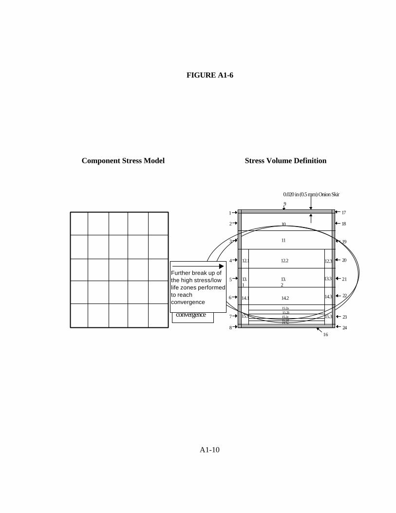
FIGURE A1-6

Component Stress Model Stress Volume Definition

Further break up of the high stress/low life

zones to reachconvergence

0.020 in (0.5 mm) Onion Skin

15.2e

15.2c

15.2a

15.2d

15.2b

16

10

14.2

13.2

12.2

17

11

9

15.3

14.3

13.3

12.3

1

2

3

4

5

6

7

8

18

19

20

21

22

23

24

12.1

13.1

14.1

15.1

A1-10

Further break up ofthe high stress/lowlife zones performedto reachconvergence

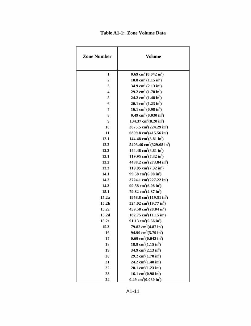
Table A1-1: Zone Volume Data

Zone Number Volume

123456789

1011

12.112.212.313.113.213.314.114.214.315.1

15.2a15.2b15.2c15.2d15.2e15.3

161718192021222324

0.69 cm3 (0.042 in3)18.8 cm3 (1.15 in3)34.9 cm3 (2.13 in3)29.2 cm3 (1.78 in3)24.2 cm3 (1.48 in3)20.1 cm3 (1.23 in3)16.1 cm3 (0.98 in3)0.49 cm3 (0.030 in3)

134.37 cm3(8.20 in3)3675.5 cm3(224.29 in3)6809.8 cm3(415.56 in3)144.48 cm3(8.81 in3)5403.46 cm3(329.68 in3)144.48 cm3(8.81 in3)119.95 cm3(7.32 in3)4488.2 cm3(273.84 in3)119.95 cm3(7.32 in3)99.58 cm3(6.08 in3)3724.1 cm3(227.22 in3)99.58 cm3(6.08 in3)79.82 cm3(4.87 in3)1958.8 cm3(119.51 in3)324.02 cm3(19.77 in3)459.58 cm3(28.04 in3)182.75 cm3(11.15 in3)91.13 cm3(5.56 in3)79.82 cm3(4.87 in3)94.90 cm3(5.79 in3)0.69 cm3(0.042 in3)18.8 cm3(1.15 in3)34.9 cm3(2.13 in3)29.2 cm3(1.78 in3)24.2 cm3(1.48 in3)20.1 cm3(1.23 in3)16.1 cm3(0.98 in3)

0.49 cm3(0.030 in3)

A1-11

(3) Step 3 - Crack Growth Model Definition. Crack growth models areconstructed for each of the zones defined in Step 2. Examples for zones 17, 22, and 10 areillustrated below in FIGURE A1-7. Guidelines for crack growth analysis are provided inFIGURE A1-2.

(a) Assumptions:

1. The crack is positioned in the most life limiting locationwithin the zone.

2. Surface anomalies are modeled as semicircular cracks.

3. Surface corner anomalies are modeled as quarter circles.

4. Subsurface anomalies are modeled as circular cracks.

FIGURE A1-7: Zone Crack Location

W i d t h = 0 . 1 m ( 3 . 9 4 i n . )T

hickness = 0.125 m (4.92 in.)

W i d t h = 0 . 1 m ( 3 . 9 4 i n . )

Thickness = 0.125 m

(4.92 in.)

Off

set =

0.1

125

m (

4.43

in.)

Z o n e 1 0

Z o n e 2 2

Z o n e 1 7

T h i c k n e s s = 0 . 1 m ( 3 . 9 4 i n . )

Wid

th =

0.0

376

m (1

.48

in.)

A1-13

(4) Step 4 - Crack Growth Calculations. Crack growth calculations areperformed (FIGURE A1-8) using the predicted stresses and crack growth rate data todetermine the residual life associated with each zone. The calculations are conducted for rangeof initial crack sizes to ensure that the component service life is covered.

(a) Assumptions:

1. All anomalies act as sharp propagating cracks and areorientated normal to the maximum principal stress: hoop stress.

2. The crack growth rate curve is the same for both surfaceand subsurface calculations.

3. Average air crack growth data.

4. No surface enhancement effects.

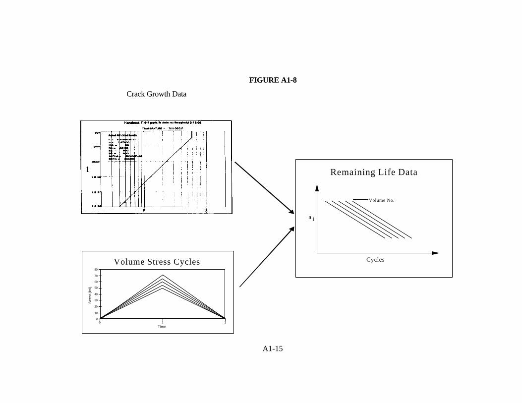
FIGURE A1-8

Crack Growth Data

Remaining Life Data

a i

Cycles

Volume No.

80

0

10

20

30

40

50

60

70

0 1 2

Time

Str

ess

(ksi

)

Volume Stress Cycles

A1-15

(5) Step 5 - Relative Risk Calculation – No In-Service Inspection. Theprobability of fracture for each stress volume is calculated integrating the volume, anomalydistribution, and residual life information from the previous steps (FIGURE A1-9). The resultsfor each zone are statistically summed to determine the total component probability of fracture.The calculated probability of fracture without an in-service inspection is 1.9 E - 09 events/cycle.

A1-16

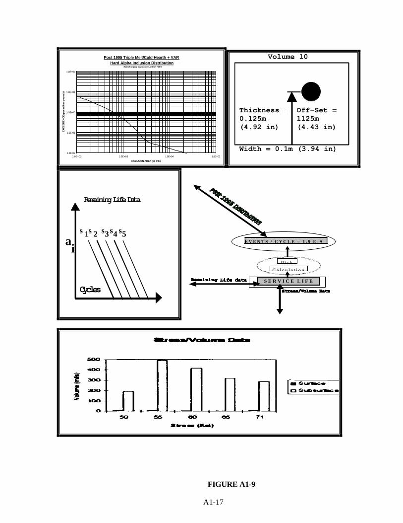
Post 1995 Triple Melt/Cold Hearth + VARHard Alpha Inclusion Distribution

1.0E-02

1.0E-01

1.0E+00

1.0E+01

1.0E+02

1.0E+02 1.0E+03 1.0E+04 1.0E+05

INCLUSION AREA (sq mils)

EX

CE

ED

EN

CE

(per

mill

ion

poun

ds)

Billet/Forging Inspections #3/#3 FBH

Width = 0.1m (3.94 in)

Thickness =0.125m(4.92 in)

Volume 10

Off-Set =1125m(4.43 in)

Remaining Life Data

ai

Cycles

σ1σ2 σ3σ4 σ5

R i s kC a l c u l a t i o n

S E R V I C E L I F E

E V E N T S / C Y C L E = 1 . 9 E - 9

FIGURE A1-9

A1-17

(6) Step 6 - Relative Risk Calculations – With a Single In-Service Inspection.The “with inspection” probability of fracture calculations are performed in the same manner as instep 5, except the ultrasonic technique (UT) inspection POD data and cycles to inspection areincluded in the risk integration (FIGURE A1-10). The calculated probability of fracture with amid-life inspection is 1.4 E - 09 events/cycle.

(a) Assumptions:

1. The UT inspection POD curve is applicable for100-percent of the component volume (surface connected and subsurface).

2. Inspection performed at 10,000 cycles.

3. Assume the anomaly area in the inspection plane isequivalent to the anomaly area in the stress plane.

A1-18

Risk

CalculationService Life

Events/Cycle = 1.4 E-9

P o s t 1 9 9 5 T r i p l e M e l t / C o l d H e a r t h + V A R

H a r d A l p h a I n c l u s i o n D i s t r i b u t i o n

B i l l e t / F o r g i n g I n s p e c t i o n s # 3 / # 3

Remaining Life Data

ai

Cycles

Inspection POD

FIGURE A1-10

A1-19

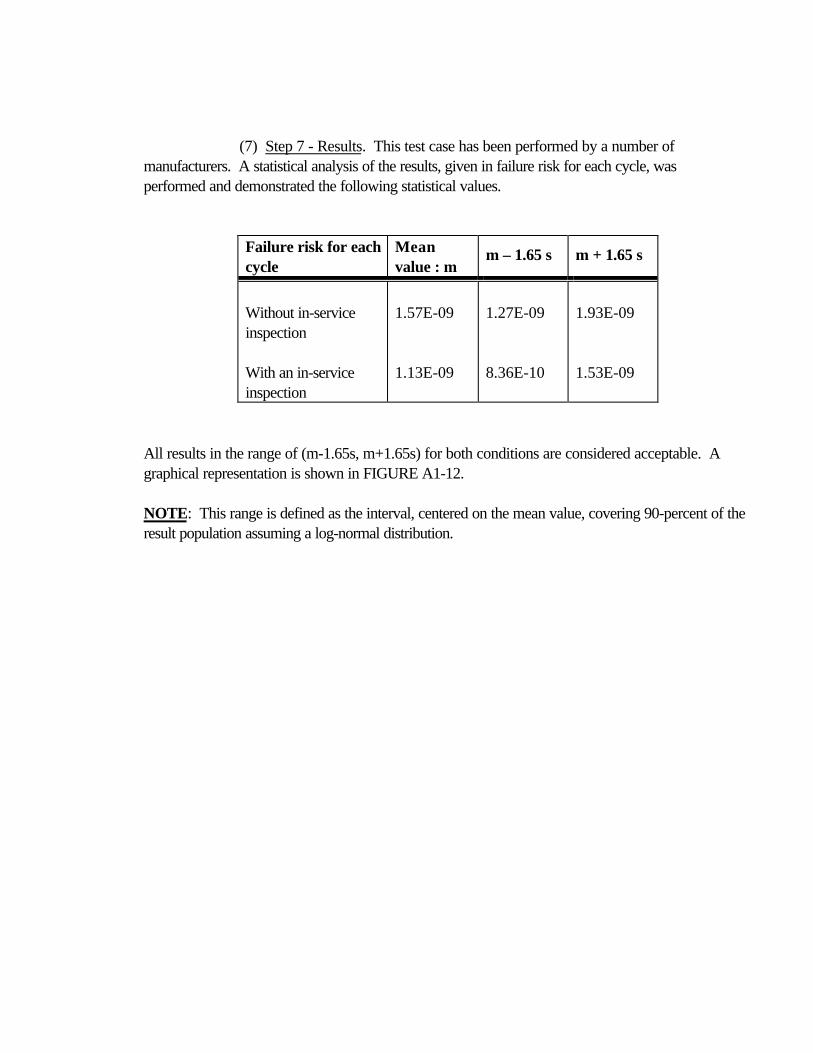
(7) Step 7 - Results. This test case has been performed by a number ofmanufacturers. A statistical analysis of the results, given in failure risk for each cycle, wasperformed and demonstrated the following statistical values.

Failure risk for eachcycle

Meanvalue : m

m – 1.65 s m + 1.65 s

Without in-serviceinspection

With an in-serviceinspection

1.57E-09

1.13E-09

1.27E-09

8.36E-10

1.93E-09

1.53E-09

All results in the range of (m-1.65s, m+1.65s) for both conditions are considered acceptable. Agraphical representation is shown in FIGURE A1-12.

NOTE: This range is defined as the interval, centered on the mean value, covering 90-percent of theresult population assuming a log-normal distribution.

FIGURE A1-11


1.0E-02

1.0E-01

1.0E+00

1.0E+01

1.0E+02

1.0E+02 1.0E+03 1.0E+04 1.0E+05

INCLUSION AREA (sq mils)

EX

CE

ED

EN

CE

(p

er m

illio

n p

ou

nd

s)


A1-21

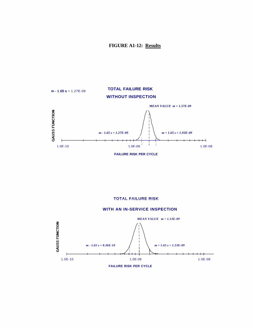
FIGURE A1-12: Results

TOTAL FAILURE RISK

WITHOUT INSPECTION

1.0E-10 1.0E-09 1.0E-08

FAILURE RISK PER CYCLE

MEAN VALUE m = 1.57E-09

m - 1.65 s = 1.27E-09 m + 1.65 s = 1.93E-09

m - 1.65 sm - 1.65 s = 1.27E-09

TOTAL FAILURE RISK

WITH AN IN-SERVICE INSPECTION

1.0E-10 1.0E-09 1.0E-08

FAILURE RISK PER CYCLE

MEAN VALUE m = 1.13E-09

m - 1.65 s = 8.36E-10 m + 1.65 s = 1.53E-09

APPENDIX 2

SOFT TIME INSPECTION EXAMPLE

1. This Appendix provides an example of an acceptable process for setting the opportunityinspection requirements that will be specified in Airworthiness Limitations Section of the Instructionsfor Continued Airworthiness. As discussed in Section 4, the application of the opportunityinspection is one of a number of options available to reduce the predicted POF in the event that acomponent design does not meet the DTR criteria.

a. Section 4 introduced the following three scenarios for opportunity inspections to clarifythe actions that could be taken at a maintenance opportunity. They are (1) Hardware available foropportunity inspection, (2) Module below soft time interval, (3) Module above soft time interval.Examples of the first and third scenarios will be presented in this Appendix, and the second scenariowould be analyzed in a similar fashion to the third scenario.

b. Key elements in determining opportunity inspection requirements given any scenario arethe type of inspection method and associated level of sensitivity, the maintenance interval at which thehardware will be exposed for inspection, and the cyclic threshold or soft time interval for moduleexposure at which time the inspections will be invoked. Given a scenario, details of an inspectionplan can take many forms. FIGURE A2-1 shows the decision process for selecting the appropriateinspection requirements. This flowchart will be referenced throughout this section to guide thediscussion.

A2-1

FIGURE A2-1In-service Inspection Decision Process

1Candidate

Design

2AssessPOF

3MeetDTR?

4Acceptable

Design

5Apply

OpportunityInspection

6Select Component

Exposure Level

7Select

InspectionThreshold

8Select

Inspection andSensitivity

- Piece Part- Module- Engine- Combination

3000 Cycles2000 Cycles1000 Cycles

- UT, #3 FBH, 1:1- UT, #3 FBH, 2:1- FPI, Full Field- EC, 1:1

9AssessPOF

12Incorporateinspectionrequirements inChapter 5 of theengine manual

11Acceptable

Design

YES

NO

YES

NO

YES

10MeetDTR?

NO(select 6, 7 or 8)

- Method- Threshold- Exposure

A2-2

2. Example of Scenario (1), Hardware Available for Opportunity Inspection.

a. It was shown in Appendix 1 that the predicted POF for the simple ring disk, without thebenefit of in-service inspection is 1.9 E-09 events/cycle (Block 2 of FIGURE A2-1). Therefore, thering disk design does not meet the 1.0 E-09 event/cycle DTR (A “No” answer at Block 3). If thering disk POF was less than the DTR, the design would be considered acceptable (Block 4) and noin-service inspection would be required.

b. Assuming a design change is not possible (for example, a reduction in stress, change inmaterial, or enhance manufacturing inspection), the decision is made (Block 5) to explore theopportunity inspection option to reduce the component risk below the DTR.

c. With the decision made to pursue the inspection route, the level of maintenanceopportunity is selected for study. The options available are piece part, module, engine, or somecombination of these opportunities. The desire is to select an exposure level or combination of levelsthat minimizes the impact on the operator, yet has a high potential of reducing the component risklevel. It is anticipated that the applicant will use trial and error to arrive at the optimum solution.However, working with this damage tolerance criteria will give the applicant experience for makinggood initial selections reducing the amount of analytical effort in future analyses. For the initial pass, aone time ultrasonic inspection (UT) at first piece part exposure (Block 6), and an inspectionthreshold of zero cycles (Block 7) will be evaluated. The piece part maintenance exposuredistribution for the ring disk is shown in FIGURE A2-2 below.

FIGURE A2-2

R i n g D i s k O v e r h a u l F i r s t P i e c e P a r t E x p o s u r eD i s t r i b u t i o n

0

2 0

4 0

6 0

8 0

1 0 0

1 2 0

0 5 0 0 0 1 0 0 0 0 1 5 0 0 0 2 0 0 0 0 2 5 0 0 0

C y c l e s

Mean = 9000 CyclesStandard Deviation = 1500

A2-3

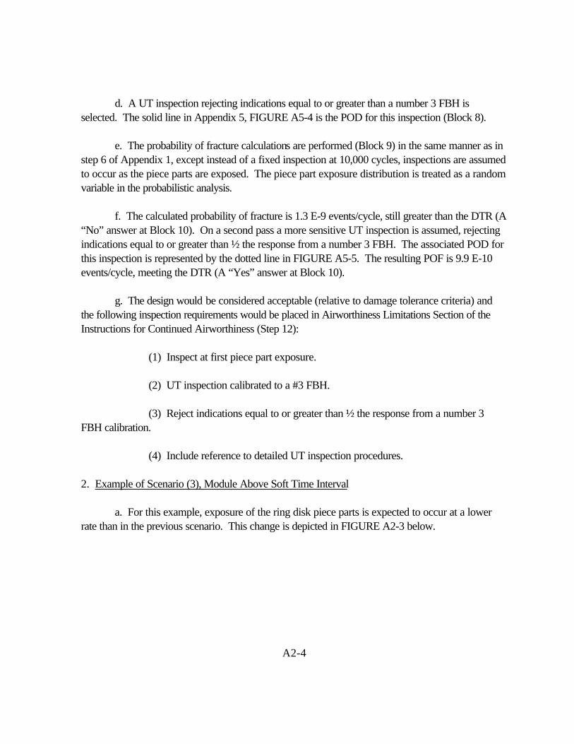
d. A UT inspection rejecting indications equal to or greater than a number 3 FBH isselected. The solid line in Appendix 5, FIGURE A5-4 is the POD for this inspection (Block 8).

e. The probability of fracture calculations are performed (Block 9) in the same manner as instep 6 of Appendix 1, except instead of a fixed inspection at 10,000 cycles, inspections are assumedto occur as the piece parts are exposed. The piece part exposure distribution is treated as a randomvariable in the probabilistic analysis.

f. The calculated probability of fracture is 1.3 E-9 events/cycle, still greater than the DTR (A“No” answer at Block 10). On a second pass a more sensitive UT inspection is assumed, rejectingindications equal to or greater than ½ the response from a number 3 FBH. The associated POD forthis inspection is represented by the dotted line in FIGURE A5-5. The resulting POF is 9.9 E-10events/cycle, meeting the DTR (A “Yes” answer at Block 10).

g. The design would be considered acceptable (relative to damage tolerance criteria) andthe following inspection requirements would be placed in Airworthiness Limitations Section of theInstructions for Continued Airworthiness (Step 12):

(1) Inspect at first piece part exposure.

(2) UT inspection calibrated to a #3 FBH.

(3) Reject indications equal to or greater than ½ the response from a number 3FBH calibration.

(4) Include reference to detailed UT inspection procedures.

2. Example of Scenario (3), Module Above Soft Time Interval

a. For this example, exposure of the ring disk piece parts is expected to occur at a lowerrate than in the previous scenario. This change is depicted in FIGURE A2-3 below.

A2-4

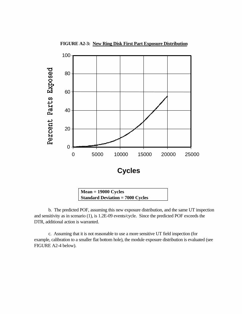
FIGURE A2-3: New Ring Disk First Part Exposure Distribution

0

20

40

60

80

100

0 5000 10000 15000 20000 25000

Cycles

Mean = 19000 Cycles Standard Deviation = 7000 Cycles

b. The predicted POF, assuming this new exposure distribution, and the same UT inspectionand sensitivity as in scenario (1), is 1.2E-09 events/cycle. Since the predicted POF exceeds theDTR, additional action is warranted.

c. Assuming that it is not reasonable to use a more sensitive UT field inspection (forexample, calibration to a smaller flat bottom hole), the module exposure distribution is evaluated (seeFIGURE A2-4 below).

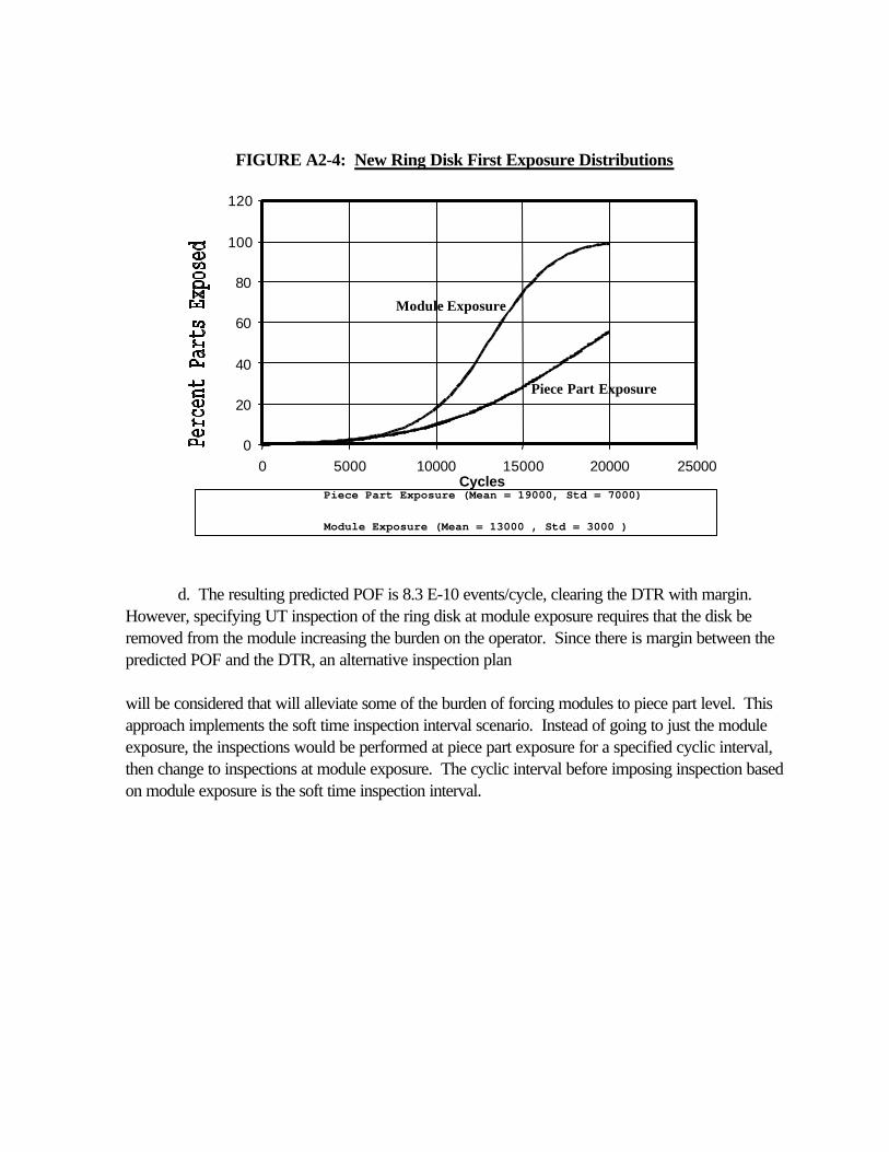
FIGURE A2-4: New Ring Disk First Exposure Distributions

Piece Part Exposure

Module Exposure

0

20

40

60

80

100

120

0 5000 10000 15000 20000 25000Cycles

Piece Part Exposure (Mean = 19000, Std = 7000)

Module Exposure (Mean = 13000 , Std = 3000 )

d. The resulting predicted POF is 8.3 E-10 events/cycle, clearing the DTR with margin.However, specifying UT inspection of the ring disk at module exposure requires that the disk beremoved from the module increasing the burden on the operator. Since there is margin between thepredicted POF and the DTR, an alternative inspection plan

will be considered that will alleviate some of the burden of forcing modules to piece part level. Thisapproach implements the soft time inspection interval scenario. Instead of going to just the moduleexposure, the inspections would be performed at piece part exposure for a specified cyclic interval,then change to inspections at module exposure. The cyclic interval before imposing inspection basedon module exposure is the soft time inspection interval.

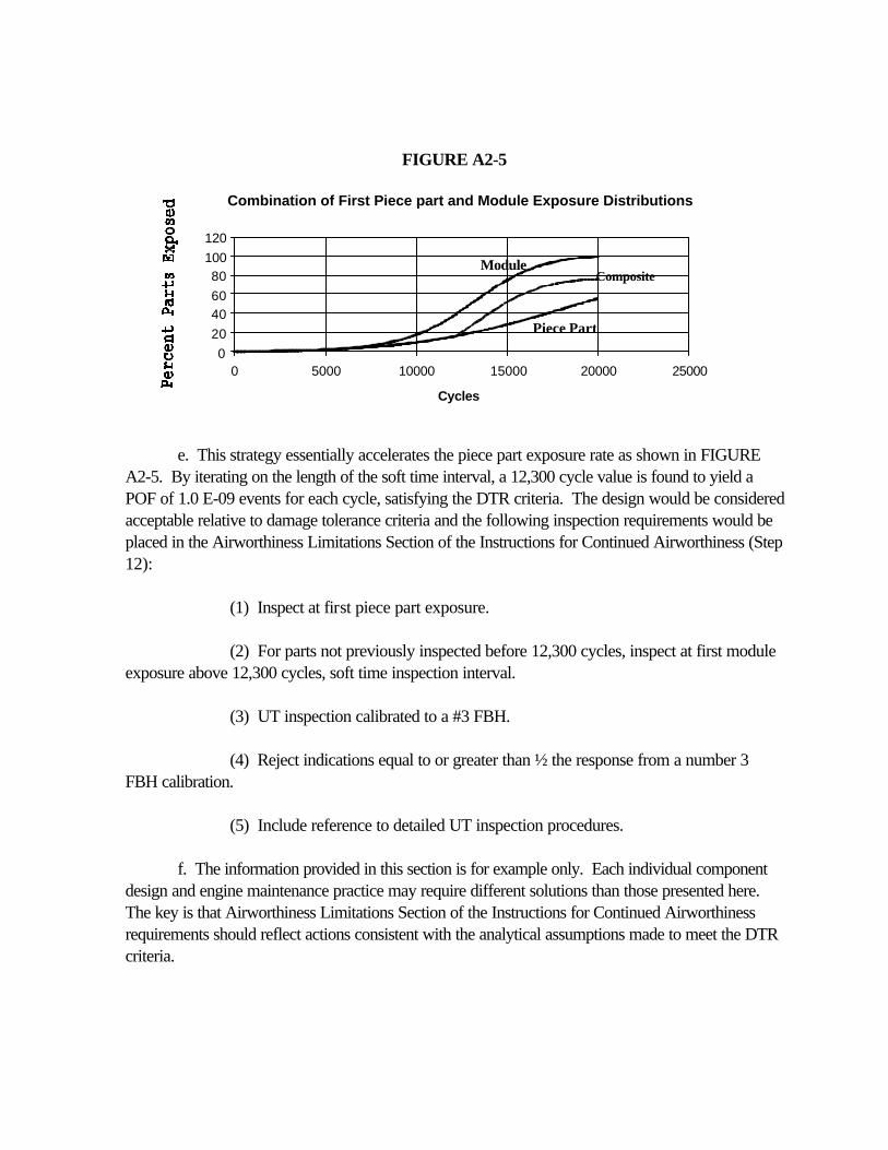
FIGURE A2-5

Piece Part

ModuleComposite

Combination of First Piece part and Module Exposure Distributions

020406080

100120

0 5000 10000 15000 20000 25000

Cycles

e. This strategy essentially accelerates the piece part exposure rate as shown in FIGUREA2-5. By iterating on the length of the soft time interval, a 12,300 cycle value is found to yield aPOF of 1.0 E-09 events for each cycle, satisfying the DTR criteria. The design would be consideredacceptable relative to damage tolerance criteria and the following inspection requirements would beplaced in the Airworthiness Limitations Section of the Instructions for Continued Airworthiness (Step12):

(1) Inspect at first piece part exposure.

(2) For parts not previously inspected before 12,300 cycles, inspect at first moduleexposure above 12,300 cycles, soft time inspection interval.

(3) UT inspection calibrated to a #3 FBH.

(4) Reject indications equal to or greater than ½ the response from a number 3FBH calibration.

(5) Include reference to detailed UT inspection procedures.

f. The information provided in this section is for example only. Each individual componentdesign and engine maintenance practice may require different solutions than those presented here.The key is that Airworthiness Limitations Section of the Instructions for Continued Airworthinessrequirements should reflect actions consistent with the analytical assumptions made to meet the DTRcriteria.

APPENDIX 3

DEFAULT ANOMALY DISTRIBUTION CURVES

1. Anomaly Distribution Curves

a. The anomaly distribution curves associated with hard-alpha inclusions in titanium enginerotors are illustrated in this Appendix (FIGURES A3-1 - A3-18). The following text providesadditional information associated with the use of these distributions.

(1) The distributions are applicable only to hard-alpha inclusions in rotor grade(premium) titanium melted after 1995 using triple VAR or CHM plus VAR processes.

(2) It is crucial to use the appropriate distribution curve that accurately reflects theinspection sensitivities performed at the billet and forging stages of the manufacturing process.

(3) For example, the material must be inspected using UT to at least a#3 FBH with the reject level set at one half that of the calibration level. See Appendix 5 foradditional instructions. Inspections must be performed at both the billet and sonic shape stages.

(4) The distribution accounts for all steps required to manufacture a finished part,including the in-process billet and sonic shape forging ultrasonic inspections. Therefore, the distributionused should reflect the inspection sensitivities used in the billet and forging inspections, and should notbe altered.

(5) Referring to the FIGURES in this Appendix:

(a) The vertical axis represents the expected number of hard-alphainclusions for each million pounds of titanium. This information should be treated as the probability ofhaving an inclusion of a given size or larger (exceedance probability).

(6) The horizontal axis is the inclusion cross-sectional area including the hard-alphacore and the surrounding diffusion zone. A circular inclusion cross section should be assumed withthe corresponding diameter used as the initial size in the crack growth analysis.

A3-1

FIGURE A3-1


Billet / Forging Inspections #5/#3 FBH

0.01

0.1

1

10

100

100 1000 10000 100000

DEFECT INSPECTION AREA (sq mils)

A3-2

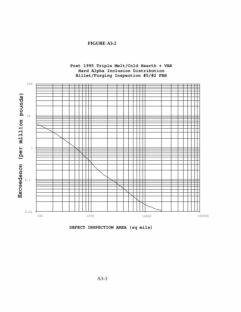
FIGURE A3-2


Billet/Forging Inspection #5/#2 FBH

0.01

0.1

1

10

100

100 1000 10000 100000


A3-3

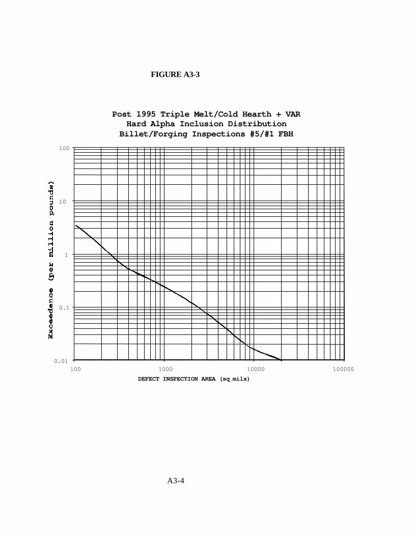
FIGURE A3-3



0.01

0.1

1

10

100

100 1000 10000 100000DEFECT INSPECTION AREA (sq mils)

A3-4

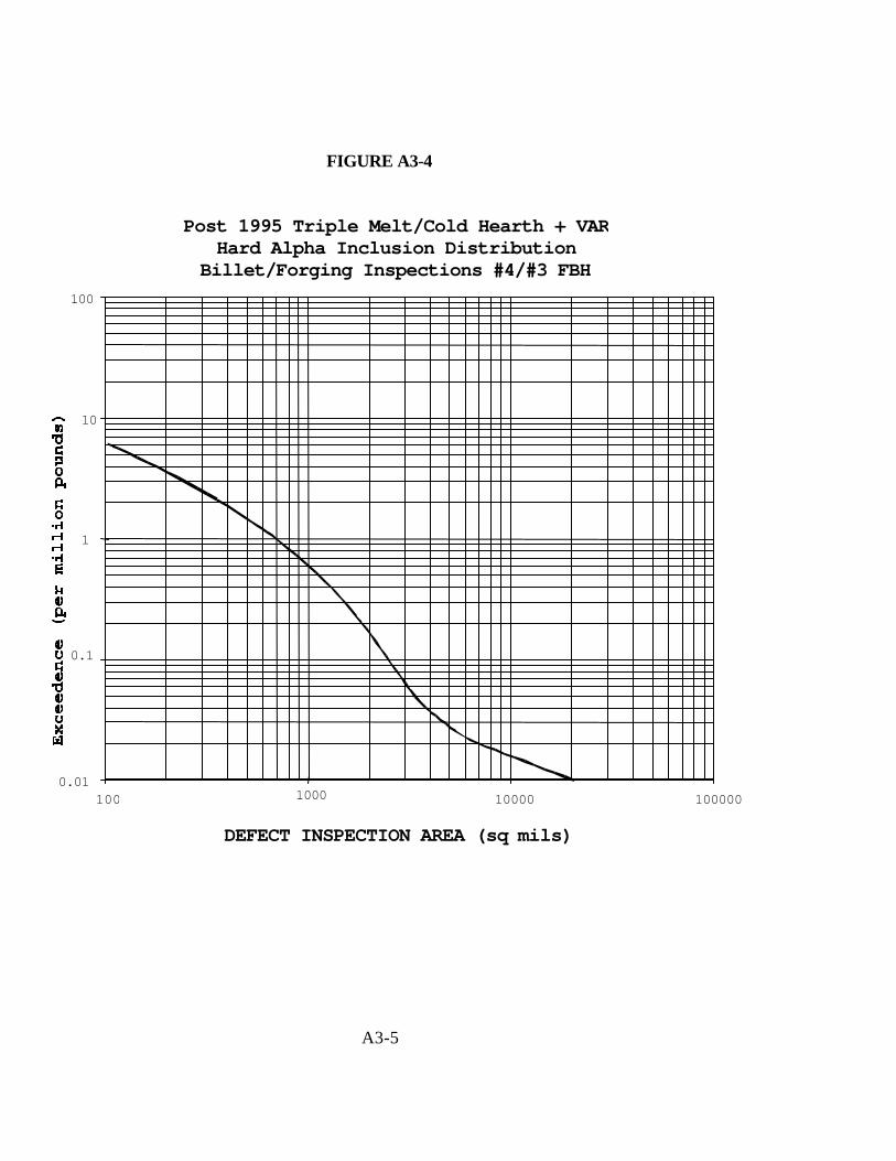
FIGURE A3-4



0.01

0.1

1

10

100

100 1000 10000 100000


A3-5

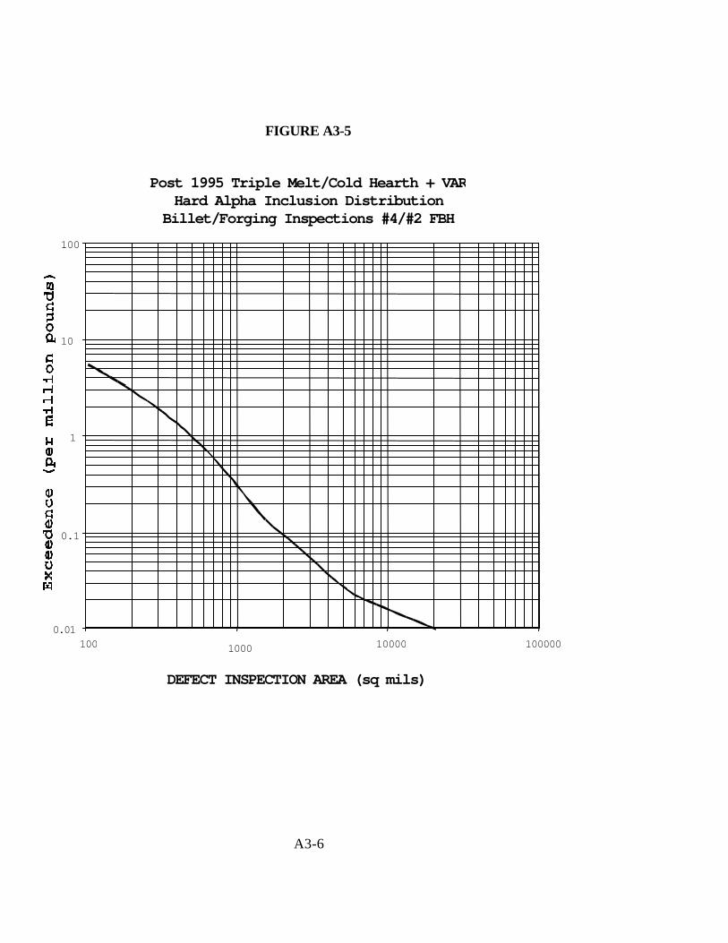
FIGURE A3-5



0.01

0.1

1

10

100

100 1000 10000 100000


A3-6

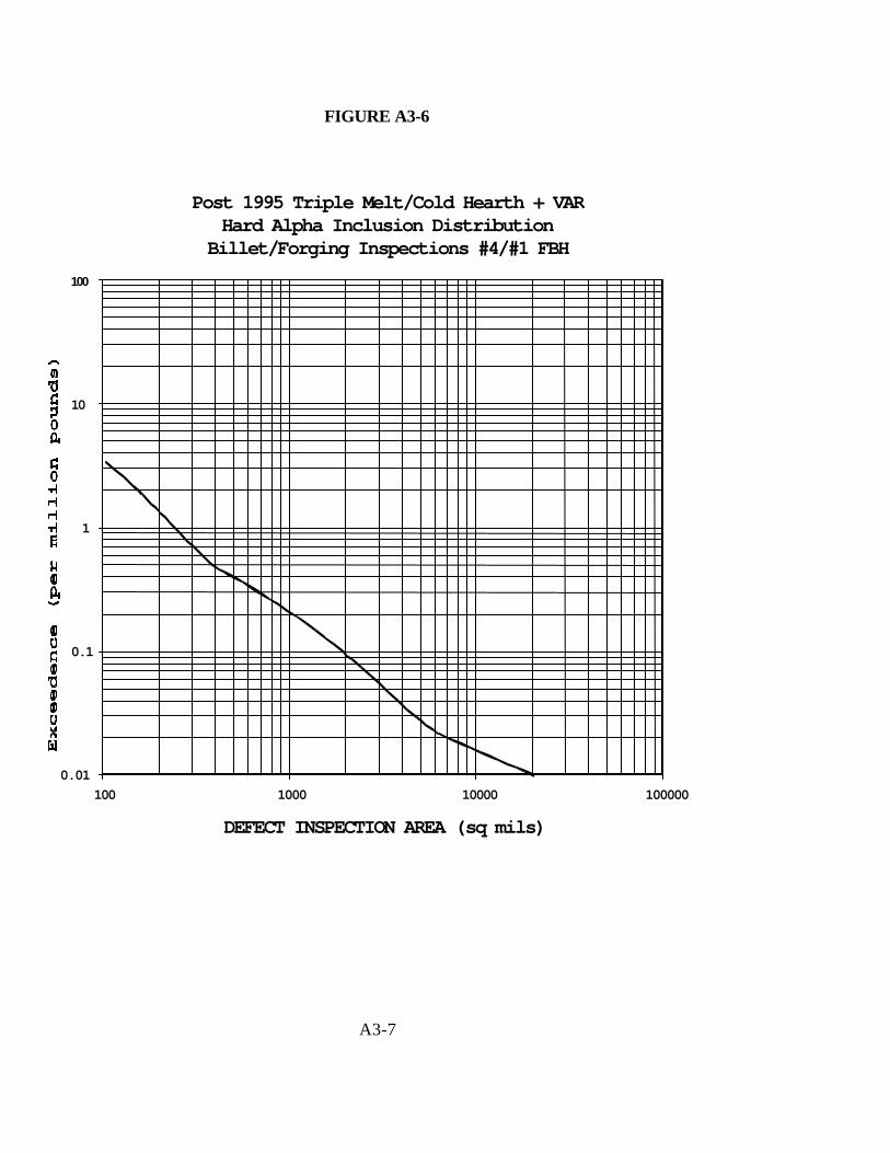
FIGURE A3-6



0.01

0.1

1

10

100

100 1000 10000 100000


A3-7

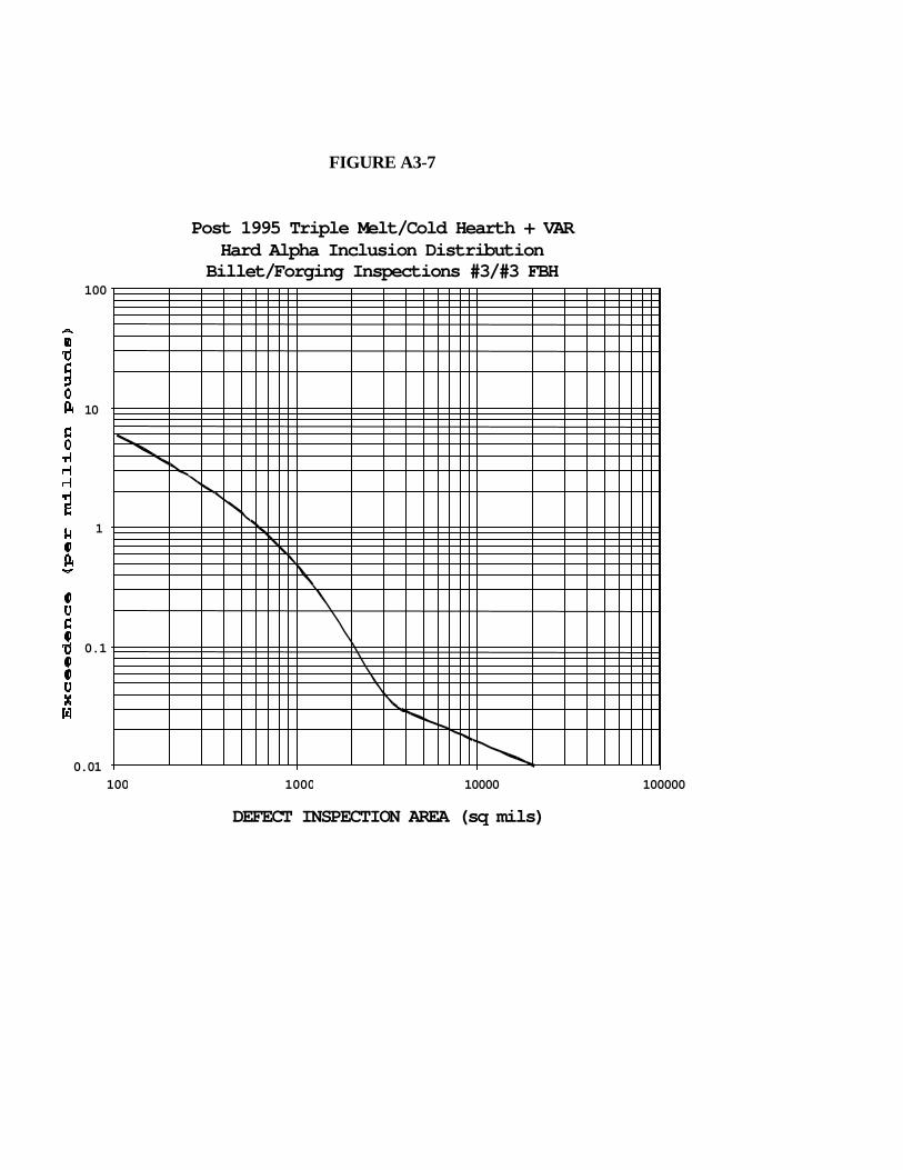
FIGURE A3-7



0.01

0.1

1

10

100

100 1000 10000 100000


FIGURE A3-8



0.01

0.1

1

10

100

100 1000 10000 100000


FIGURE A3-9



0.01

0.1

1

10

100

100 1000 10000 100000


A3-10

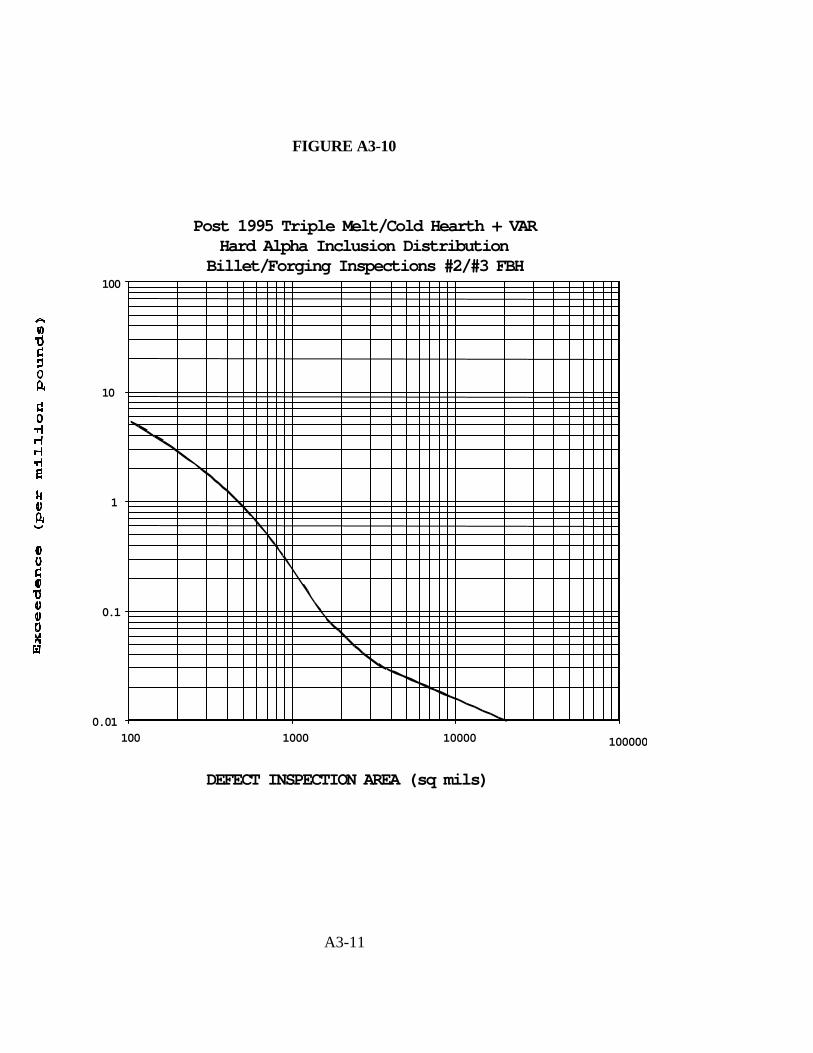
FIGURE A3-10



0.01

0.1

1

10

100

100 1000 10000 100000


A3-11

FIGURE A3-11



0.01

0.1

1

10

100

100 1000 10000

100000


A3-12

FIGURE A3-12

Post 1995 Triple Melt/Cold Hearth + VARHard Alpha Inclusion DistributionBillet/Forging Inspections #2/#1

0.01

0.1

1

10

100

100 1000 10000 100000


FIGURE A3-13


Billet/Forging Inspections MZ (12-13" billet)/#3 FBH

0.01

0.1

1

10

100

100 1000 10000 100000


FIGURE A3-14


Billet / Forging Inspections MZ (12-13" Billet)/#2 FBH

0.01

0.1

1

10

100

100 1000 10000 100000


A3-15

FIGURE A3-15



0.01

0.1

1

10

100

100 1000 10000 100000


FIGURE A3-16



0.01

0.1

1

10

100

100 1000 10000 100000


A3-17

FIGURE A3-17



0.01

0.1

1

10

100

100 1000 10000 100000


FIGURE A3-18



0.01

0.1

1

10

100

100 1000 10000 100000


A3-19

APPENDIX 4

DEFAULT POD APPLICABILITY

1. Use of Default POD Data

a. This Appendix defines conditions relevant to the use of accepted estimates of theprobability of detection (POD) for specific types of anomalies and specific nondestructiveevaluation/inspection techniques, which may be considered as default values when applied underappropriately similar conditions. The conditions defined in this Appendix do not necessarilyguarantee the validity of these POD values. For example, if inspection parameters, such as penetrantconcentration or temperature, are inadequately controlled, the penetrant capability shown in theaccompanying graph will not be attained, even if the correct penetrant is selected. Use of a writtenplan for controlling and monitoring inspection processes is recommended (see paragraph 3 of thisAppendix).

b. If the conditions described for each inspection are not satisfied, the resultant inspectioncapability and reliability will be reduced. Accordingly, the use of the default POD values would thenbe inappropriate and would result in an overly optimistic damage tolerance assessment.

2. Demonstrations of Inspection Capability

a. For ECI and ultrasonic inspection techniques, alternative default POD curves are given.Choice of the appropriate POD curve must be based on demonstration that the stated calibrationand reject signal levels are attainable on the component being inspected, and, for example, notprevented by noise or geometrical features. The demonstration conditions should be appropriate tothe properties of the part inspected that may affect the inspectability, such as surface conditions,depth to be inspected, proximity to edges, etc. No other demonstration of these default capabilitiesis necessary, as long as the requirements for the specific inspection technique are satisfied (seeparagraphs 3-6 of this Appendix).

b. It should be noted that, for specific inspection techniques applied under well controlledconditions, it may be possible to achieve POD values that are significantly better than the defaultPOD values. Advantage may be taken of any such improved capability and reliability only if it issupported by a well documented demonstration

A4-1

program. Similarly, a well documented demonstration program may be necessary in order tomeasure POD values appropriate to specific conditions that are excluded from those the defaultvalues is supported by explicit, reasonable assumptions.

3. General Restrictions and Applicability

a. The inspection process must be well controlled, and performed in accordance withacceptable procedures, such as those defined by the engine standard practices manual, andconsistent with good industrial inspection practices, such as those defined by MIL-STD’s, orequivalent industry standards.

b. Pertinent inspection process parameters such as coverage, probe indexing, and scanningspeeds (see paragraph 4 of Section 3, and paragraphs 4-6 of this Appendix), should be governed bywritten procedures;. Inspection plans and any inspection fixturing, should be designed to minimizehuman and other sources of variability.

c. Inspectors must be fully qualified and trained for each MIL-STD-410, ASNT-TC-1A,ATA-105, or equivalent, and provided with adequate training instructions in the specific inspectionmethod.

d. The default POD data presented in this AC are applicable only to titanium alloys used forengine disks, and only to inspected material. Geometrical conditions, such as radii and edges cancreate areas where inspections can not be accomplished. Limitations also exist relative to depth ofpenetration and near surface resolution. Conditions under which the default POD data wereacquired are outlined in paragraphs 4-6 of this Appendix; advice about the equivalence of alternativeconditions should be sought from those with expertise in NDE. Areas of high compressive residualstress can have negative effects on the capability of various NDE techniques, most notably penetrantinspection.

e. Applicability of the default POD data is limited to components exhibiting no abnormalsurface conditions, and that have been properly cleaned for each shop manual requirements. Noother special pre-inspection cleaning or polishing is required.

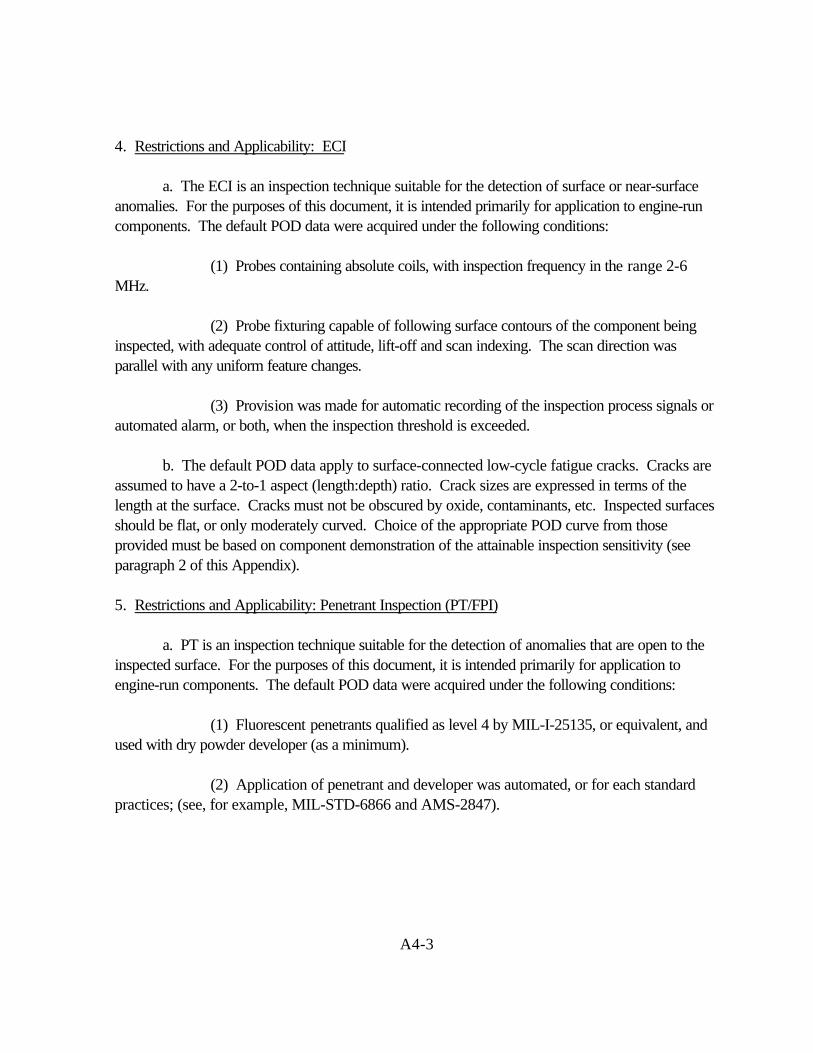
4. Restrictions and Applicability: ECI

a. The ECI is an inspection technique suitable for the detection of surface or near-surfaceanomalies. For the purposes of this document, it is intended primarily for application to engine-runcomponents. The default POD data were acquired under the following conditions:

(1) Probes containing absolute coils, with inspection frequency in the range 2-6MHz.

(2) Probe fixturing capable of following surface contours of the component beinginspected, with adequate control of attitude, lift-off and scan indexing. The scan direction wasparallel with any uniform feature changes.

(3) Provision was made for automatic recording of the inspection process signals orautomated alarm, or both, when the inspection threshold is exceeded.

b. The default POD data apply to surface-connected low-cycle fatigue cracks. Cracks areassumed to have a 2-to-1 aspect (length:depth) ratio. Crack sizes are expressed in terms of thelength at the surface. Cracks must not be obscured by oxide, contaminants, etc. Inspected surfacesshould be flat, or only moderately curved. Choice of the appropriate POD curve from thoseprovided must be based on component demonstration of the attainable inspection sensitivity (seeparagraph 2 of this Appendix).

5. Restrictions and Applicability: Penetrant Inspection (PT/FPI)

a. PT is an inspection technique suitable for the detection of anomalies that are open to theinspected surface. For the purposes of this document, it is intended primarily for application toengine-run components. The default POD data were acquired under the following conditions:

(1) Fluorescent penetrants qualified as level 4 by MIL-I-25135, or equivalent, andused with dry powder developer (as a minimum).

(2) Application of penetrant and developer was automated, or for each standardpractices; (see, for example, MIL-STD-6866 and AMS-2847).

A4-3

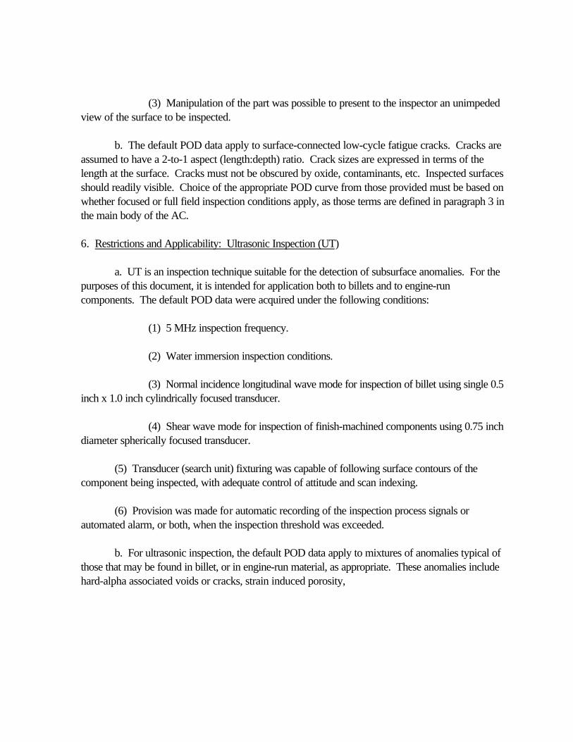
(3) Manipulation of the part was possible to present to the inspector an unimpededview of the surface to be inspected.

b. The default POD data apply to surface-connected low-cycle fatigue cracks. Cracks areassumed to have a 2-to-1 aspect (length:depth) ratio. Crack sizes are expressed in terms of thelength at the surface. Cracks must not be obscured by oxide, contaminants, etc. Inspected surfacesshould readily visible. Choice of the appropriate POD curve from those provided must be based onwhether focused or full field inspection conditions apply, as those terms are defined in paragraph 3 inthe main body of the AC.

6. Restrictions and Applicability: Ultrasonic Inspection (UT)

a. UT is an inspection technique suitable for the detection of subsurface anomalies. For thepurposes of this document, it is intended for application both to billets and to engine-runcomponents. The default POD data were acquired under the following conditions:

(1) 5 MHz inspection frequency.

(2) Water immersion inspection conditions.

(3) Normal incidence longitudinal wave mode for inspection of billet using single 0.5inch x 1.0 inch cylindrically focused transducer.

(4) Shear wave mode for inspection of finish-machined components using 0.75 inchdiameter spherically focused transducer.

(5) Transducer (search unit) fixturing was capable of following surface contours of thecomponent being inspected, with adequate control of attitude and scan indexing.

(6) Provision was made for automatic recording of the inspection process signals orautomated alarm, or both, when the inspection threshold was exceeded.

b. For ultrasonic inspection, the default POD data apply to mixtures of anomalies typical ofthose that may be found in billet, or in engine-run material, as appropriate. These anomalies includehard-alpha associated voids or cracks, strain induced porosity,

etc. It should be noted that other anomaly types may occur, such as high density inclusions, butthese are not included in the current analysis. Anomaly sizes are expressed in terms of maximumcross-sectional area perpendicular to the sound beam, including associated diffusion zones whereappropriate.

c. Inspected finish-machined surfaces should be flat, or only moderately curved. Billetsshould be circular-cylindrical, and in customary pre-inspection conditions (turned, ground, orpeeled).

d. Choice of the appropriate POD curve from those provided must be based on componentdemonstration of the attainable inspection sensitivity (see paragraph 2 of this Appendix). Provisionmust be made to maintain this sensitivity at all depths, and effective distance-amplitude compensationis required.

APPENDIX 5

DEFAULT POD CURVES

FIGURE A5-1

POD FOR FLUORESCENT PENETRANT INSPECTION OFFINISH-MACHINED SURFACES

0

10

20

30

40

50

60

70

80

90

100

10 100 1000

ANOMALY LENGTH (mils)

Full-field inspection Directed inspection

Applicability:

MIL-I-25135 Level 4 penetrants with dry powder developer (as minimum)

A5-2

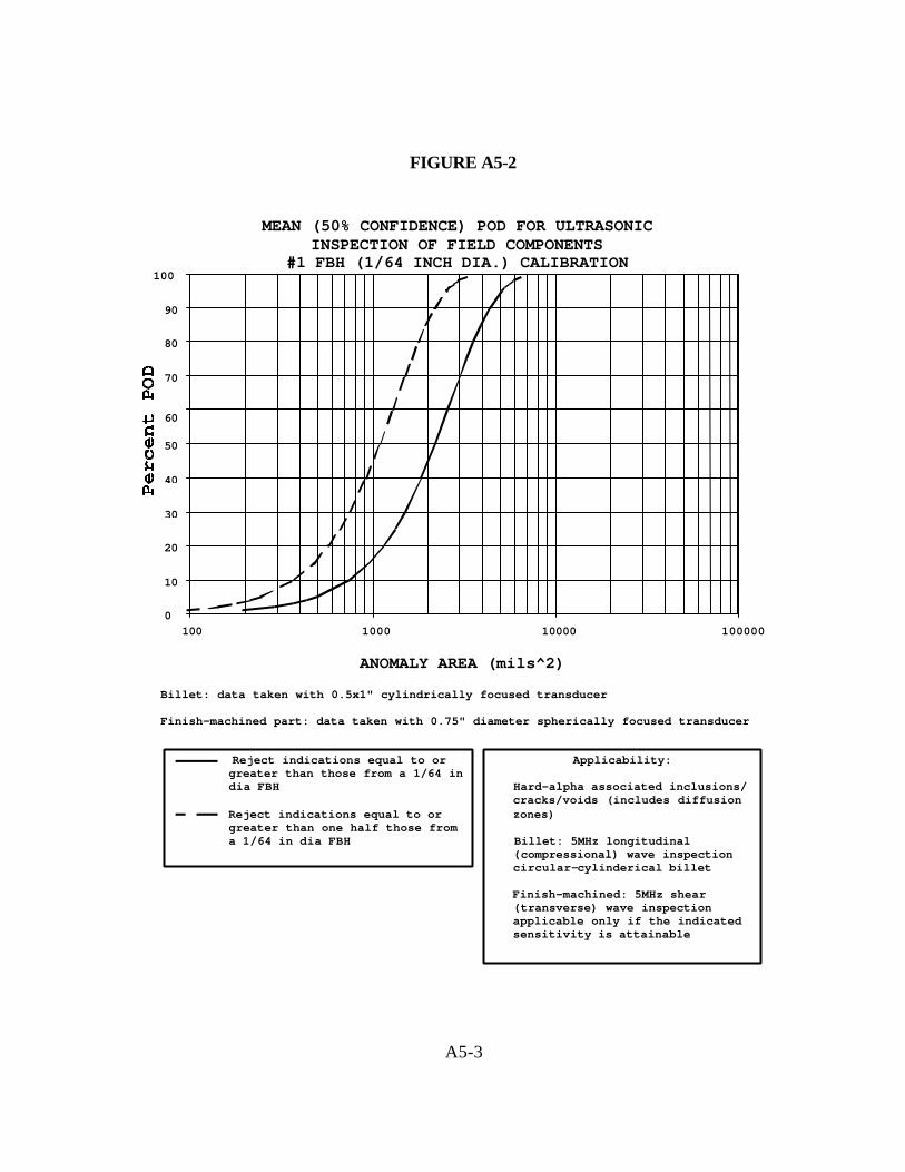
FIGURE A5-2

MEAN (50% CONFIDENCE) POD FOR ULTRASONICINSPECTION OF FIELD COMPONENTS

#1 FBH (1/64 INCH DIA.) CALIBRATION

0

10

20

30

40

50

60

70

80

90

100

100 1000 10000 100000

ANOMALY AREA (mils^2)

Billet: data taken with 0.5x1" cylindrically focused transducer

Finish-machined part: data taken with 0.75" diameter spherically focused transducer

Reject indications equal to or greater than those from a 1/64 in dia FBH

Reject indications equal to or greater than one half those from a 1/64 in dia FBH

Applicability:

Hard-alpha associated inclusions/ cracks/voids (includes diffusion zones)

Billet: 5MHz longitudinal (compressional) wave inspection circular-cylinderical billet

Finish-machined: 5MHz shear (transverse) wave inspection applicable only if the indicated sensitivity is attainable

A5-3

FIGURE A5-3

MEAN (50% CONFIDENCE) POD FOR ULTRASONICINSPECTION OF FIELD COMPONENTS


0

10

20

30

40

50

60

70

80

90

100

100 1000 10000 100000






Applicability:

Hard-alpha associated inclusions/ cracks/ voids (includes diffusion zones)


Finish-machined: 5MHz shear (transverse) wave inspection

Applicable only if the indicated sensitivity is attainable

A5-4

FIGURE A5-4

MEAN (50% CONFIDENCE) POD FOR ULTRASONIC INSPECTION OFFIELD COMPONENTS


0

10

20

30

40

50

60

70

80

90

100

100 1000 10000 100000






Applicability:

Hard-alpha associated inclusions/ cracks/ voids (includes diffusion zones)


Finish-machined: 5MHz shear (transverse) wave inspection applicable only if the indicated sensitivity is attainable

A5-5

FIGURE A5-5

MEAN (50% CONFIDENCE) POD FOR EDDY CURRENT OFFINISH-MACHINED SURFACES

0

10

20

30

40

50

60

70

80

90

100

10 100

ANOMALY LENGTH (mils)

Reject at the calibration notch threshold response and above

Reject at one half the calibration notch threshold response and above

Applicabilty:

Absolute coils, 2-6 MHz inspection frequency

Calibration on 0.030" x 0.015" notch applicable only if the indicated sensitivity is attainable

A5-6

subject: date: ac no: engine rotors initiated by: change...

Documents