subject: date: ac no: engine rotors initiated by: … · 1/8/01 . ac no: engine rotors . initiated...

Subject: Damage Tolerance for High Energy Turbine Date: 1/8/01 AC No:Engine Rotors Initiated By: AC 33.14-1

ANE-110 Change:

1. PURPOSE.

a. This advisory circular (AC) describes an acceptable means for showing compliance with the requirements of § 33.14 of the Federal Aviation Regulations (Title 14, Code of Federal Regulations). Section 33.14 contains requirements applicable to the design and life management of high energy rotating parts of aircraft gas turbine engines.

b. Like all advisory material, this AC is not, in itself, mandatory, and does not constitute a regulation. It is issued to describe an acceptable means, but not the only means, for demonstrating compliance applicable to the design and life management of titanium alloy high energy rotating parts of aircraft gas turbine engines. Terms such as "shall" and "must" are used only in the sense of ensuring applicability of this particular method of compliance when the acceptable method of compliance described in this document is used.

c. This AC does not change, create any additional, authorize changes in, or permit deviations from the existing regulatory requirements.

2. RELATED READING MATERIAL.

a. FAA Advisory Circular: AC 33.2B, titled “Aircraft Engine Type Certification Handbook”.

b. FAA Advisory Circular: AC 33.3, titled “Turbine and Compressor Rotor Type Certification Substantiation Procedures”.

c. FAA Advisory Circular: AC 33.4, titled “Design Consideration Concerning the use of Titanium in Aircraft Turbine Engines”.

d. FAA Advisory Circular: AC 33.15, titled “Manufacturing Process of Premium Quality Titanium Alloy Rotating Engine Components”.

AC 33.14-1 1/8/01

3. DEFINITIONS.

a. Component Event Rate. The number of events for a given titanium rotor component stage for each flight cycle, calculated over the projected life of the component.

b. Critical Rotating Parts. Rotor structural parts (such as disks, spools, spacers, hubs, and shafts), the failure of which could result in a hazardous condition. In this context a hazardous condition should be interpreted as the conditions described in § 33.75.

c. Damage Tolerance. This is an element of the life management process that recognizes the potential existence of component imperfections. The potential existence of component imperfections are the result of inherent material structure, material processing, component design, manufacturing or usage. Damage tolerance addresses this situation through the incorporation of fracture resistant design, fracture-mechanics, process control, or nondestructive inspection.

d. Default Probability of Detection (POD) Values. Values representing mean probabilities of detecting anomalies of various types and sizes, under specified inspection conditions consistent with good industry practice.

e. Design Target Risk (DTR) Value. This is the standard against which probabilistic assessment results (stated in terms of component event rates and engine level event rates, as defined below) are compared.

f. Engine Event Rate. The cumulative number of events for each flight cycle, for all critical titanium rotating parts in a given engine, calculated over the projected life of those components.

g. Event. A rotor structural part separation, failure, or burst with no regard to the consequence.

h. Focused Inspection. A term used to describe inspections in which any necessary specialized processing instructions have been provided, and the inspector has been instructed to pay attention to specific critical features.

i. Full Field Inspection. A term used to describe the general inspection of a component without special attention to any specific features.

Par 3

1/8/01 AC 33.14-1

j. Hard-Alpha or High Interstitial Defect (HID). An interstitially stabilized alpha phase region of substantially higher hardness than the surrounding material. This comes from very high local nitrogen, oxygen, or carbon concentrations, which increase the beta transus and produce the high hardness, often brittle, alpha phase; also commonly called a Type I defect, low density inclusion (LDI), or a hard-alpha; often associated with voids and cracks.

k. Hard Time Inspection Interval. The number of flight cycles since new or the most recent inspection, after which a rotor part must be made available and receive the inspection specified in the Airworthiness Limitations Section of the Instructions for Continued Airworthiness.

l. Inspected Material. That portion of the total volume of a component that is actually inspected under the described conditions. Inspected material does not guarantee anomaly free material.

m. Inspection Opportunity. An occasion when an engine is disassembled to at least the modular level and the hardware in question is accessible for inspection, whether or not the hardware has been reduced to the piece part level.

n. Low Cycle Fatigue (LCF) Initiation. The process of progressive and permanent local structural deterioration occurring in a material subject to cyclic variations, in stress and strain, of sufficient magnitude and number of repetitions. The process will culminate in detectable crack initiation typically within 105 cycles. For the purposes of this AC, a detectable crack initiation is defined as 0.030 inches in length by 0.015 inches in depth.

o. Maintenance Exposure Interval. Distribution of shop visits (in-flight cycles) since new or last overhaul that an engine, module, or component is exposed to as a function of normal maintenance activity.

p. Mean POD. The 50-percent confidence level POD versus anomaly size curve.

q. Module Available. An individual module removed from the engine.

r. Module. A combination of assemblies, subassemblies, and parts contained in one package, or arranged to be installed in one maintenance action.

Par 3

AC 33.14-1 1/8/01

s. Part Available. A part that can be inspected, as required by the Airworthiness Limitations Section of the Instructions for Continued Airworthiness, without any further disassembly. Depending on the inspection requirements, some parts may require a fully disassembled “piece part” condition, while other parts may be available for inspection while still in the assembled module.

t. Probabilistic (Relative Risk) Assessment. A fracture-mechanics based simulation procedure that uses statistical techniques to mathematically model and quantitatively combine the influence of two or more variables to estimate a most likely outcome or range of outcomes for a product. Since not all variables may be considered or may not be capable of being accurately quantified, the numerical predictions are used on a comparative basis to evaluate various options having the same level of inputs. Results from these analyses are typically used for design optimization to meet a predefined target, or to conduct parametric studies. This type of procedure is distinctly different from an absolute risk analysis, which attempts to consider all significant variables, and is used to quantify, on an absolute basis, the predicted number of future events having safety and reliability ramifications.

u. POD. A quantitative statistical measure of detecting a particular type of anomaly over a range of sizes using a specific nondestructive inspection technique under specific conditions. Typically, the mean POD curve is used.

v. Safe-Life. A LCF based process where components are designed and substantiated to have a specified service life, which is stated in operating cycles or operating hours, or both. Continued safe operation, up to the stated life limit is not contingent upon each unit of a given design receiving interim inspections. When a component reaches its published life limit, it is retired from service.

w. Soft Time Inspection Interval. The number of flight cycles since new or the most recent inspection, after which a rotor part in an available module must receive the inspection specified in the Airworthiness Limitations Section of the Instructions for Continued Airworthiness.

x. Stage. The rotor structure which supports, and is attached to a single aerodynamic blade row.

1/8/01 AC 33.14-1

4. BACKGROUND.

a. Service experience with gas turbine engines has demonstrated that material and manufacturing anomalies do occur. These anomalies can potentially degrade the structural integrity of high energy rotors. Conventional rotor life management methodology (safe-life method) is founded on the assumption of the existence of nominal material variations and manufacturing conditions. Consequently, the methodology does not explicitly address the occurrence of such anomalies, although some level of tolerance to anomalies is implicitly built-in using design margins, factory and field inspections, etc.

b. Under nominal conditions, this safe-life methodology provides a structured process for the design and life management of high energy rotors, which results in the assurance of structural integrity throughout the life of the rotor. Undetectable material processing and manufacturing induced anomalies, therefore, represent a departure from the assumed nominal conditions. In 1990, to quantify the extent of such occurrences the FAA requested that the Society of Automotive Engineers (SAE) reconvene the ad hoc committee on uncontained events. The statistics pertaining to uncontained rotor events are reported in the SAE committee report Nos. AIR 1537, AIR 4003, and SP-1270. While no adverse trends were identified, the committee expressed concern that the projected 5-percent increase in airline passenger traffic each year would lead to a noticeable increase in the number of aircraft accidents from uncontained rotor events. Uncontained rotor events have the potential to cause catastrophic aircraft accidents.

c. As a result of the accident at Sioux City in 1989, the FAA requested the turbine engine manufacturers, through the Aerospace Industries Association (AIA), to review available techniques to determine if a damage tolerance approach could be introduced which, if appropriately implemented, could reduce the occurrence of uncontained rotor events.

d. The industry working group concluded that the technology was now available to implement additional enhancements to the conventional rotor life management process, which would explicitly address anomalous conditions. Furthermore, these enhancements could be structured to enforce design and life management adaptations, which would enhance rotor integrity under anomalous material or manufacturing conditions. The additional guidelines regarding damage tolerance provided in this AC explicitly address these anomalous conditions. In addition, the damage tolerance approach will also implicitly enhance damage tolerance to other anomalous conditions related to design, manufacture, maintenance and operation.

Par 4 Page 5

AC 33.14-1 1/8/01

5. APPLICABILITY.

a. This material has been prepared to present a generic damage tolerance approach which can be readily integrated with the existing “safe-life” process for high energy rotors to produce an enhanced life management process. However, the data included in this AC are only applicable to titanium alloy rotor components.

b. This material is intended to be applicable to all “new design” critical titanium alloy rotor components on a “go forward basis.” It is not intended to apply retroactively to existing hardware.

c. The new generic damage tolerance approach does not replace existing safe-life methodology, but expands upon it.

d. In the context of damage tolerance, it is not intended to allow operation beyond the component manual limit set using the existing safe-life approach.

e. Rotor failure modes for which full containment can be demonstrated are excluded from the procedures outlined in this document and need not be accounted for in the overall risk assessment.

/s/ David A. Downey Assistant Manager, Engine & Propeller Directorate Aircraft Certification Service

CONTENTS

Page No.

Section 1 Conventional (“Safe-Life”) Life Management Process S1-1

Section 2 Enhanced Life Management Process S2-1

Section 3 Damage Tolerance Implementation S3-1

- Approach

- Methodology

- Default Input - Anomaly Distributions

- Default Input - Nondestructive Evaluation (NDE) Probability of Detection (POD)

- Design Target Risk (DTR)

Section 4 “Soft-Time Inspection” Rotor Life Management Approach S4-1

Section 5 References S5-1

APPENDICES

Appendix 1 Calibration Test Case & Example Damage Tolerance Assessment A1-1

Appendix 2 Soft Time Inspection Interval Example A2-1

Appendix 3 Default Anomaly Distribution Curves A3-1

Appendix 4 Default POD Applicability A4-1

Appendix 5 Default POD Curves A5-1

SECTION 1

CONVENTIONAL (“Safe-Life”) LIFE MANAGEMENT PROCESS

1. The conventional gas turbine engine critical rotor life management methodology (the “safelife” method) consists of comprehensive processes and technologies related to the design, manufacture, test validation, certification and field management of high energy rotors. FIGURE S1-1 illustrates the basic elements of the safe-life approach to rotor life management. Taken together, these processes and technologies constitute a procedure approved by the FAA as fulfilling the requirements of § 33.14 for the type certification of aircraft engines under part 33.

a. Analytical and empirical engineering processes are applied to determine statistically quantified LCF-based minimum rotor service lives. The minimum lives are reflective of service usage profiles associated with specific applications.

b. Structured component and engine testing is conducted to confirm rotor operating conditions and to enhance confidence in the predicted minimum service lives.

c. Controlled and fixed processes are established for the manufacture of critical rotors as part of the safe-life process. These manufacturing processes are formalized in addition to the product definition data. Periodic quality validation testing is used to assure product quality consistent with intended design.

d. Certification of declared lives is established as a fraction of the minimum LCF life, with the fractional ratio dependent upon the approved safety factors associated with the particular application. The declared lives and supporting engineering data are submitted to the FAA for review and approval as part of the overall type certification process. Upon FAA approval, the certificated critical rotor life limits are documented in the Airworthiness Limitations Section of the Instructions for Continued Airworthiness, and becomes an operational limit. After introduction into operational service, the FAA may approve increases to the critical rotor certificated life limits if the engine manufacturer can validate the proposed increases with sufficient supporting data. The FAA may also order decreases to the certificated life under part 39 when warranted.

e. Critical rotors are retired through scheduled operator maintenance action, before or upon reaching the certificated life limit.

f. Opportunity inspections, as part of the normal maintenance practices, are another element of the conventional life management process. Even though the approval of certificated life limits is not contingent upon interim or even periodic inspections, most of the critical rotors do become available for inspection several times as part of normal engine maintenance practices.

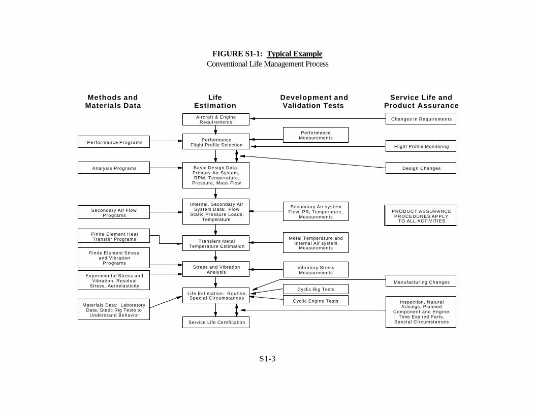
FIGURE S1-1: Typical Example Conventional Life Management Process

Methods and Life Development and Service Life and Materials Data Estimation Validation Tests Product Assurance

Performance Programs

Analysis Programs

Secondary Air Flow Programs

Finite Element Heat Transfer Programs

Finite Element Stress and Vibration

Programs

Experimental Stress and Vibration, Residual

Stress, Aeroelasticity

Materials Data: Laboratory Data, Static Rig Tests to

Understand Behavior

Performance Flight Profile Selection

Basic Design Data: Primary Air System, RPM, Temperature,

Pressure, Mass Flow

Internal, Secondary Air System Data: Flow

Stat ic Pressure Loads, Temperature

Transient Metal Temperature Estimation

Stress and Vibration Analysis

Life Estimation: Routine, Special Circumstances

Service Life Certification

Aircraft & Engine Requirements

Vibratory Stress Measurements

Cyclic Rig Tests

Cyclic Engine Tests

Changes in Requirements

Flight Profile Monitoring

Design Changes

Manufacturing Changes

Inspection, Natural Arisings, Planned

Component and Engine, Time Expired Parts,

Special Circumstances

Performance Measurements

Secondary Air system Flow, PR, Temperature,

Measurements

Metal Temperature and Internal Air system

Measurements

PRODUCT ASSURANCE PROCEDURES APPLY

TO ALL ACTIVITIES

S1-3

g. The requirements for life estimation are represented by the elements in FIGURE S11. Life limits are to be specified for any engine rotor component where a failure of that component would result in a hazard to the aircraft. Within the cyclic life span, it is assumed that continued safe operation of the specific rotor design, up to the stated life limit, is not contingent upon interim or periodic inspections. The key elements of life estimation include:

(1) Flight Cycle Definition: A flight cycle should be defined that considers the most severe and typical operation of the engine. The flight cycle provides the operational definition so that the stress and thermal analyses can capture the transient and cyclical loading. The part lives are quoted in terms of this flight cycle. The flight cycle should include the various flight segment such as start, idle, takeoff, climb, cruise, approach, landing, reverse and shutdown. The hold times at the various flight segments should correspond to the limiting installation variables (aircraft weight, climb rates, etc.). The corresponding rotor speeds, internal pressures, and temperatures during each flight segment should be adjusted to account for production tolerances and installation trim procedures, as well as engine deterioration that can be expected between heavy maintenance intervals. The range of ambient temperature and takeoff altitude conditions encountered during the engines’ service life should also be considered.

(2) Thermal Analysis: The flight cycle along with the corresponding performance data, act as boundary conditions for the thermal analysis. Temperature levels and thermal gradients should be determined throughout the flight cycle and should be calibrated and verified by engine rotor temperature data.

(3) Stress Analysis: Analytical and empirical engineering processes are applied to determine the stress distribution for each structural part. The analyses evaluate the effects of engine speed, pressure, metal temperature and thermal gradients at many discrete flight cycle conditions. From this, the component’s cyclic stress history is constructed. Stress concentration effects due to geometric discontinuities such as dovetails, boltholes and contour changes should be included.

(4) Life Prediction System: The life prediction system is based upon test data obtained from cyclic testing of specimens and components fabricated from representative production grade material to account for the manufacturing processes that affect LCF capability. Sufficient testing should be performed to evaluate the effects of elevated temperatures and hold times, as well as, interaction with other material failure mechanisms such as high cycle fatigue (HCF) and creep. Test data should be reduced statistically in order to express the results in terms of minimum LCF capability (1/1000 or alternately -3 sigma) and the safe-life should be quoted to initiation of a fatigue crack. Appropriate prior service experience gained through a successful program of parts retirement or precautionary sampling inspections, or both, may be included to expand the database.

SECTION 2

ENHANCED LIFE MANAGEMENT PROCESS

1. History has shown that the safe-life philosophy has served the turbine engine industry and flying public well, and provides a solid base for further enhancement. Modifications to the conventional life management procedures should augment, not supplant, current approaches, which are based on the safe-life philosophy.

a. By adding a new element, damage tolerance, to the existing conventional life management process, the enhanced life management process has been defined to further minimize the occurrence of uncontained rotor failures and thus improve flight safety (see FIGURE S2-1).

b. Use of the enhanced life management process depicted in FIGURE S2-1, will result in damage tolerance assessments being conducted on critical titanium alloy rotor designs. These will be fracture-mechanics based probabilistic risk assessments, the results of which will be compared to the agreed upon design target risk (DTR) values. Designs that satisfy these DTR values will be considered to comply with the requirements of § 33.14. The engine manufacturer will have a variety of options available to achieve the DTR values. They include, but are not limited to, component redesign, material changes, material process improvements, manufacturing inspection improvements, in-service inspections, and life limit reductions.

c. A general methodology for conducting the fracture-mechanics based probabilistic analyses mentioned above is presented in Section 3 (Damage Tolerance Implementation).

S2-1

FIGURE S2-1: Enhanced Life Management Process

Safe Life Prediction

Methods & Material Data

Development & Validation

Tests

Life Management Process

Damage Tolerance

Assessment

New Element Added to

Existing Safe Life Process

Service Life & Product Assurance

SECTION 3

DAMAGE TOLERANCE IMPLEMENTATION

1. Approach

a. Fracture-mechanics based probabilistic (FMBP) assessments are a key feature of the enhanced life management process. The results of these assessments will provide the basis for evaluating the relative damage tolerance capabilities of candidate engine designs, and will also allow the engine manufacturer to balance the designs for both enhanced reliability and customer impact. The results will be compared against agreed upon DTR values (see paragraph 5 of this Section).

b. The necessity for further risk reducing actions on the part of the engine manufacturer will be based upon whether or not the design under consideration satisfies the desired DTR values at both the individual component level and the overall engine level. If the targets are met, then the design is considered to comply with § 33.14. The manufacturer may conduct quantitative parametric studies to determine the influence of key variables such as inspection methods, inspection frequency, hardware geometry, hardware processing, material selection and life limit reduction. The manufacturer may then make changes to the design or field management of the part, or both, in order to achieve the agreed upon DTR values, as shown in FIGURE S3-1. This approach provides the individual engine manufacturer with the flexibility to develop an optimal engine design solution consistent with customer requirements and company policies, procedures, and available resources. An example assessment utilizing this methodology is described in paragraph 2 of this Section, and provided in Appendix 1 of this AC.

c. FMBP assessments will usually be performed during the engine component detail design phase. Paragraph 2 of this Section defines an assessment methodology applicable to material melt-related induced anomalies. It contains a standardized list of inputs for conducting FMBP assessments, and a process to refine a design to achieve the desired DTR values.

2. Methodology

a. Probabilistic risk assessments may be conducted using a variety of methods, such as Monte Carlo simulation or numerical integration techniques; the methodology

S3-1

and assumptions used to determine the risk should be approved by the FAA. FIGURE S3-1 conceptually depicts a melt-related anomaly probabilistic assessment. When performing an FMBP assessment, use of the standardized inputs and default data presented in this AC will achieve consistent FMBP assessment results across the industry.

b. A list of standardized inputs is provided below. Default input data is described in paragraphs 3 and 4 of this Section. Use of this default data in probabilistic assessments requires no further demonstration of applicability or accuracy. However, where this data is used, the guidelines accompanying this data should be followed by the engine manufacturer to ensure applicability. Use of input other than these default values may require additional validation to verify applicability, adequacy, and accuracy.

c. Probabilistic risk assessments should incorporate the following inputs as part of a basic analysis: component stress and volume, material properties, crack growth lives, anomaly distribution, design service life, inspection PODs, and maintenance exposure rate.

(1) Input. The following criteria are defined as basic input data.

(a) Anomaly Distribution. For melt-related (hard-alpha) assessments, use the default anomaly distributions outlined in paragraph 3 of this Section, or FAA approved company-specific data. Company-specific data should be developed using the same process employed to derive the default anomaly distributions. This process is described in a technical paper titled “Development of Anomaly Distributions for Aircraft Engine Titanium Disk Alloys” (see Section 5). Anomalies will be treated as sharp propagating cracks from the first stress cycle.

(b) POD. Default PODs and instructions on use of individual company values are contained in paragraph 4 of this Section. Subsurface assessments should consider the effects of ultrasonic inspection only. Surface assessments should likewise consider the effects of fluorescent penetrant inspection (FPI) and eddy-current inspection (ECI).

(c) Maintenance Exposure Interval. For the purpose of assessing inspection benefits, exposure interval curves for the engine, module, or component in question should be modeled in the analysis.

(d) Stress. Variable influencing crack propagation life. Input should encompass the most limiting operational principal stresses. Subsurface

S3-2

assessments should incorporate the appropriate subsurface and near surface stress distribution. Surface assessments should incorporate the appropriate surface stress distributions, including the effects of stress concentration. Flight cycle(s) for design LCF certification, or actual usage (if known) should be used to establish the stress profile. The influence of major and minor cycles needs to be considered since the cyclic damage accumulation can be dramatically different for crack propagation as opposed to initiation. Note that the method described in this AC has been calibrated against industry experience without consideration for the effect of surface enhancements such as shot peening on the predicted crack propagation lives. As a result, it is inappropriate to include the beneficial effects of such enhancements on any calculations at this time. This issue may be addressed in future revisions of this document.

(e) Volume. Affects the probability of having a defect in the material. Represents the volume of material at a specific level of stress. For subsurface assessments, represents the volume of material at various levels of subsurface stress. Surface assessments should incorporate volume constituting a thin layer ("onion skin") around the surface of the part. Where a non-axisymmetric feature, such as a series of holes in a disk web has a localized stress concentration, the decision on whether it makes a significant contribution to the probability of burst must be based on the combination of mass of material at high stress and the size of the anomaly which would cause the part not to reach its safe declared life. While the method described in this AC assumes axisymmetric features, a non-axisymmetric feature can be included by reducing the cross-sectional area to ensure that the total volume when integrated around the whole circumference is equal to the volume at high stress.

(f) Materials Data. Average cyclic crack growth rate properties of the base material generated in an air environment, should be used as the default condition to calculate anomaly propagation life.

(g) Propagation Life. Number of cycles for a given size anomaly to grow to a critical size. Based upon knowledge of part stress, temperature, geometry, stress gradient, anomaly orientation, and materials properties. Linear elastic fracture-mechanics should be used for the calculation of propagation life. Default conditions should assume anomalies to be in the worst orientation to the stress field.

(2) Calibration

(a) Each engine manufacturer should calibrate its analytical prediction tools by conducting the industry test case detailed in Appendix 1. The test

S3-3

case consists of a probabilistic analysis of a simulated titanium ring disk, using specified inputs and scenarios. Test case results in the ranges from 1.27E-09 to 1.93E-09 (for the “no inspection” case) and from 8.36E-10 to 1.53E-09 (for the “with in-service inspection” case) are considered acceptable. Test case results outside of these ranges may indicate problems with either the probabilistic assessment technique or the assumptions made.

(3) Output

(a) Component Level Assessments. The probabilistic assessments and prediction of event potential should be calculated over the entire anticipated service life of the part. This result should be expressed as the number of predicted events for each cycle, and be designated as the predicted “component event rate”. For multiple stage components such as spools, the assessment should be conducted for each stage. The predicted component event rate should then be compared to the component level DTR value to assess design acceptability.

(b) Engine Level Assessments. Once all critical titanium rotors in a given engine configuration have satisfied the component level DTR value, the cumulative event rate for these components should be calculated and compared to the engine level DTR value for acceptability.

(4) General Comments. At this time, standardized inputs and default data for FMBP assessments are available only for titanium material melt-related (hard-alpha) anomalies. Future updates to this AC may include material anomaly information for other rotor grade materials such as Nickel as well as inputs and default data for manufacturing and maintenance induced anomalies. The corresponding default data for DTR values for titanium materials are specified in paragraph 5 of this Section.

(a) The FAA strongly encourages engine manufacturers to incorporate fracture resistant design concepts where possible. Credit may be given for fracture resistant or burst resistant engine design features that clearly demonstrate, through both analysis and test, a reduction in the potential for rotor failure due to the presence of unanticipated material melt induced anomalies.

(b) Because the design of an aircraft turbine engine rotor is a lengthy process involving numerous iterations, each of which can substantially alter the initial calculated DTR values, it is important that the DTR values be satisfied at the time of engine certification. Some FMBP assessments may also occur several years after the engine enters service because of such influences as design changes associated with in-service problems or changes in the analytical results due to evolving predictive capability. It is important to state here that the DTR values should be satisfied at both the individual component and overall engine levels throughout the life of the hardware.

C o m p o n e n t

Des ign I te ra t ions

Probabi l is t ic A s s e s s m e n t

Pred ic ted even ts Events /Eng. F l igh t Cyc le

F l igh t Cyc le

Peak S t ress Cond i t i on

Par t Des ign L i fe

FIGURE S3-1: Typical Elements of a Titanium Melt Related Anomaly Risk Assessment

3. Anomaly Distributions. A key input distribution associated with FMBP assessments is the size and rate of occurrence of the anomalies. This type of information is statistical in nature and can be presented in a form that plots number of inclusions that exceed a particular size in a specified amount of material.

a. Titanium Melt-Related (Hard-Alpha) Distributions.

(1) Hard-alpha anomaly distributions that apply to fully machined components have been developed to characterize a type of inclusion found in titanium (See Appendix 3). The distributions are applicable to titanium rotor components manufactured after 1995; using the triple vacuum arc remelt (VAR) process or, the cold hearth melt (CHM) plus VAR processes. For example, FIGURE A3-7 represents the anomaly distribution for a component which was inspected at both the billet and the sonic shape to at least a #3 FBH (flat bottom hole).

(2) The anomaly distributions contained in Appendix 3 may be used to determine compliance with paragraph 5 of this Section, DTR requirements. The background of the development of these distributions are contained in a technical paper titled “Development of Anomaly Distributions for Aircraft Engine Titanium Disk Alloys.” Briefly stated, the distributions were developed by modeling a complex series of interrelated steps that simulated the entire component manufacturing process from billet conversion to final machining. The final distributions were validated based on field experience. This process resulted in a number of distributions that could be used to determine a relative risk reduction, but not an absolute level of risk.

(3) Individual engine manufacturers who desire to utilize an alternate anomaly distribution or an improved inspection should use the methodology contained in reference No. 5 of Section 5 to create the alternate distributions. The alternate distribution must be substantiated by the appropriate background data. An alternate distribution should include the following: (a) three dimensional inclusion data, (b) inspection POD data, (c) should account for potential undetected, uncracked and unvoided inclusions, and (d) should be based upon substantial field experience.

b. Manufacturing/Maintenance Induced Anomaly Distributions. At the present time, there are no default data distributions for use in FMBP assessments for manufacturing or maintenance based anomalies.

S3-7

c. Rotor Grade Materials Other Than Titanium Alloy. At the present time, there are no default data distributions for use in FMBP assessments for rotors made of materials other than titanium alloy.

4. Default Input - POD by Nondestructive Evaluation (NDE).

a. The capability of individual NDE processes, such as eddy-current, penetrant, or ultrasonic inspection for the detection of local material anomalies (discontinuities or potential anomalies), is a function of numerous parameters, including the size, shape, orientation, location, and chemical or metallurgical character of the anomaly. In addition, the following four parameters should be considered when assessing the capabilities of an NDE process:

(1) The material being inspected (such as its composition, grain size, conductivity, surface texture, etc.).

(2) The inspection materials or instrumentation (such as the specific penetrant and developer, the inspection frequency, instrument bandwidth and linearity, etc.).

(3) The inspection parameters (such as scan index).

(4) The inspector (such as visual acuity, attention span, training, etc.).

b. The “default” POD data supplied with this AC are characteristic of inspection capability that has been measured under typical, well controlled conditions. These default POD values are provided primarily to facilitate selection of nondestructive inspection techniques that are best suited to support attainment of damage tolerant inspections. It must be recognized that, although properly applied inspections should result in capability similar to these default values, they are strictly applicable only under the conditions under which they were acquired (see Appendix 4). If exacting use is to be made of these data, skilled professional judgment as to their applicability will be necessary. POD curves are described in Appendix 5, FIGURES A51-A5-5, as listed below:

(1) Appendix 5, FIGURE A5-1. Mean POD for Fluorescent Penetrant Inspection of Finish-Machined Surfaces.

S3-8

(2) Appendix 5, FIGURE A5-2. Mean POD for #1 FBH Ultrasonic Inspection of Field Components.



(5) Appendix 5, FIGURE A5-5. Mean POD for Eddy-Current Inspection of Finish Machined Surfaces.

NOTE: Refer to Appendix 1 for an example of the use of this data, and Appendix 4 for the NDE Applicability of these POD curves.

5. Design Target Risk (DTR).

a. The DTR is an agreed upon benchmark risk level selected to enhance the overall safety of high energy titanium rotating components. Since no machine or device is 100-percent reliable, it is inappropriate to require a level that is technologically unachievable. Nevertheless, the goal is to achieve a significant and distinct improvement over and above current rotor designs.

b. Representative “Component level DTRs” and an “engine level DTR” for titanium hard-alpha anomalies have been established based on improvements of the data presented in the SAE report. These DTRs represent consensus values, developed from assessments on representative component designs using the methodology and inputs (described in paragraphs 1-4 of Section 3). The “component level DTR” corresponds to the maximum allowable predicted component event rate. The “engine level DTR” corresponds to the maximum allowable (cumulative) component event rate for all critical titanium rotating parts in a given engine.

c. Designs must satisfy the component level DTR and the engine level DTR to be considered acceptable.

(1) Application. Default DTR values have been established for melt related (hard-alpha) anomalies. Calculated event rates should be assessed against the

appropriate DTR values. For multiple stage components, such as spools, each individual stage must satisfy the component level DTR value.

(2) Default DTR values for titanium alloys:

(a) Melt related (hard-alpha) anomalies:

component level DTR: 1 x 10-9 events/flight cycle engine level DTR: 5 x 10-9 events/flight cycle

(b) Manufacturing or Maintenance Induced Surface Anomalies: At the present time, there are no default DTR values for manufacturing or maintenance related surface anomalies.

(3) Default DTR Values for Other Than Titanium Alloy: At the present time, there are no default DTR values for other than titanium alloys.

SECTION 4

“SOFT TIME INSPECTION” ROTOR LIFE MANAGEMENT

1. Approach. The overall life management process encompasses a wide spectrum of design, manufacture, and product support issues. This section addresses only one facet of that overall process, namely the assurance of structural integrity using inspection techniques and intervals derived from a damage tolerance (fracture-mechanic based) assessment. The inspection philosophy is solely intended to protect against anomalous conditions. It is not intended to allow operation beyond the safe-life limit specified in the Airworthiness Limitations Section of the Instructions for Continued Airworthiness.

a. In instances where probabilistic assessment indicates risk levels greater than the desired target, many strategies can be utilized to reduce the predicted risk to the appropriate level. However, only the in-service inspection option is addressed here.

b. The industry data on uncontained fracture experience summarized in SAE reports AIR 1537 (1959 through 1975), AIR 4003 (1976 through 1983), and SP1270 (1984 through 1989) was used to guide the development of the inspection philosophy. These reports indicate that the maintenance induced uncontained failure rates were comparable to the failure rates for anomalous conditions (material and manufacture). This data suggests that additional inspection requirements, if not properly integrated into the normal maintenance scheduled for the engine, would have no net benefit to the uncontained failure rates.

c. The inspection philosophy presented here evolved from the desire to have inspections easily integrated into the operation of the engine yet achieve measurable reduction in the uncontained failure rates. The inspection philosophy advocates the use of opportunity inspections rather than forced inspections at ‘not to exceed’ intervals. These opportunity inspections occur due to the ‘on condition’ maintenance practices used by operators today. Although the opportunity inspections occur at random intervals, they can be treated statistically and used effectively to lower the calculated risk of an uncontained event.

d. Opportunity inspection refers to those instances when the hardware in question is available in a form such that the specified inspection can be performed. This condition

S4-1

is generally viewed as being reduced to the piece part; however; opportunity inspections can be performed on assembled modules. For example, an ECI of a disk bore may be specified on an assembled module whenever the module is available. This inspection is an opportunity inspection based upon module availability rather than piece part availability.

e. Whenever possible, the designs should use opportunity inspections to meet the DTR levels. However, in some instances, the probabilistic analysis may indicate unacceptable risk level when using just opportunity inspections and some additional action may be required to meet the DTR. One of the many options to mitigate this risk is to force inspection opportunities by specifying disassembly of modules or engines when a cyclic life interval has been exceeded. There are many options on how to implement the forced disassembly. The options range from mandatory engine removal and subsequent teardown at not to exceed cyclic limits (“hard-time” limits) to mandatory module teardown when the naturally occurring module availability exceeds the specified cyclic life inspection interval of one of the parts contained within that module (“soft-time” limits). This AC only advocates the use of the soft-time inspection option when forced disassembly of modules is required to meet the DTR levels.

f. The soft-time inspection philosophy retains the “on-condition” maintenance practice and minimizes the impact of additional module disassembly. The inspection requirement comes into effect only after the engine has been removed from the aircraft for a reason other than the inspection itself, and is in a sufficient state of disassembly to afford access to the module containing the component in question. An available module containing a part with cycles since last inspection (CSLI) in excess of the soft-time interval will be required to be disassembled to a condition that allows inspection by the procedure specified by the engine manufacturer. The risk associated with parts that become available for inspection before the soft-time interval must be evaluated by the engine manufacturer to determine if the CSLI can be reset.

g. The maintenance impact of the soft-time intervals should be considered during the design phase. The probabilistic analysis summarized in Section 3 should be used along with the anticipated engine removal rate and the module and piece part availability to develop designs that achieve the design target, but also result in acceptable soft-time intervals and procedures, should such action be required.

h. When invoked, the soft-time inspection approach establishes interval limits beyond which rotor components must be inspected when the rotors are available in modular form. The soft-time inspection requirement is not intended to impact or modify

S4-2

current practice of forced inspection programs to address safety of flight concerns that arise in the course of engine operation and maturation. These safety of flight concerns would continue to be addressed through aggressive inspection programs which are mandated through Airworthiness Directives (ADs).

i. It is important to recognize that the inspection assumptions made in the probabilistic risk assessment must be communicated and implemented accurately to the field by using the Airworthiness Limitations Section of the Instructions for Continued Airworthiness, and be validated by the review of engine removal rates and module and piece part availability data. For example, the Airworthiness Limitations Section must call out an immersion ultrasonic inspection if that was an assumption in setting the original soft-time interval. Similarly, the amount of inspected material should correspond to the analysis assumptions. Likewise, if the field experience suggests that the opportunity inspection intervals are in excess of the assumed rates in the probabilistic risk assessment, then appropriate corrective action, such as a modified inspection plan, is required.

j. The soft-time inspection interval and reference to the corresponding inspection procedures will be specified in the Airworthiness Limitations Section of the Instructions for Continued Airworthiness. This information is to be provided for all rotor parts with specified retirement life limits that require any inspection plans beyond opportunity inspections to meet the DTR levels. The required inspection information should also be included in the individual Airworthiness Limitations Section of the Instructions for Continued Airworthiness with the other rotor inspection requirements. The manufacturer will also provide necessary information to focus the prescribed inspections to those areas of highest relative risk.

2. Inspection Scenarios.

a. The following scenarios clarify the action that would be taken at a maintenance inspection opportunity. Note that the inspection plans may vary for each part, depending on the outcome of the probabilistic assessments.

(1) Maintenance Opportunity - Hardware Available For Opportunity Inspection: Hardware available in the condition to perform the specified opportunity inspection must be inspected by the procedures specified in the Airworthiness Limitations Section of the Instructions for Continued Airworthiness. This would be a mandatory inspection.

S4-5

(2) Maintenance Opportunity - Module Below Soft Time Interval: Hardware accessible in the assembled or partially disassembled module may be nondestructively inspected by the procedures specified in the Airworthiness Limitations Section of the Instructions for Continued Airworthiness. The CSLI may be reset to zero, provided the engine manufacturer has assessed the risk impact associated with this action. This would be a discretionary inspection.

(3) Maintenance Opportunity - Module Above Soft Time Interval: Hardware listed in Airworthiness Limitations Section of the Instructions for Continued Airworthiness must be made available for nondestructive inspection, using the procedures that are specified. This inspection must be performed whenever the module is available and the CSLI for any contained hardware that exceeds the inspection cycle limit. This would be a mandatory inspection.

S4-6

SECTION 5

REFERENCES

1. SAE/FAA Committee On Uncontained Turbine Engine Rotor Events, Report No. AIR 1537, Data Period 1962-1975.

2. SAE/FAA Committee On Uncontained Turbine Engine Rotor Events, Report No. AIR 4003, Data Period 1976-1983.

3. SAE/FAA Committee On Uncontained Turbine Engine Rotor Events, Report No. SP1270, Data Period 1984-1989.

4. FAA Advisory Circular 33.15, “Manufacturing Process of Premium Quality Titanium Alloy Rotating Engine Components,” September 22, 1998.

5. “Development of Anomaly Distributions for Aircraft Engine Titanium Disk Alloys” Technical paper was presented by the AIA Rotor Integrity Sub-Committee at the American Institute of Aeronautics and Astronautics (AIAA) Conference in April 1997.

APPENDIX 1

CALIBRATION TEST CASE

1. This Appendix provides a self contained package for calibration of a probabilistic risk assessment methodology. The package includes all required input data for the test case, analysis guidelines, and a test case analysis section that permits manufacturers to estimate the level of acceptability of their risk calculations and gain insights on intermediate results.

2. Test Case Input data

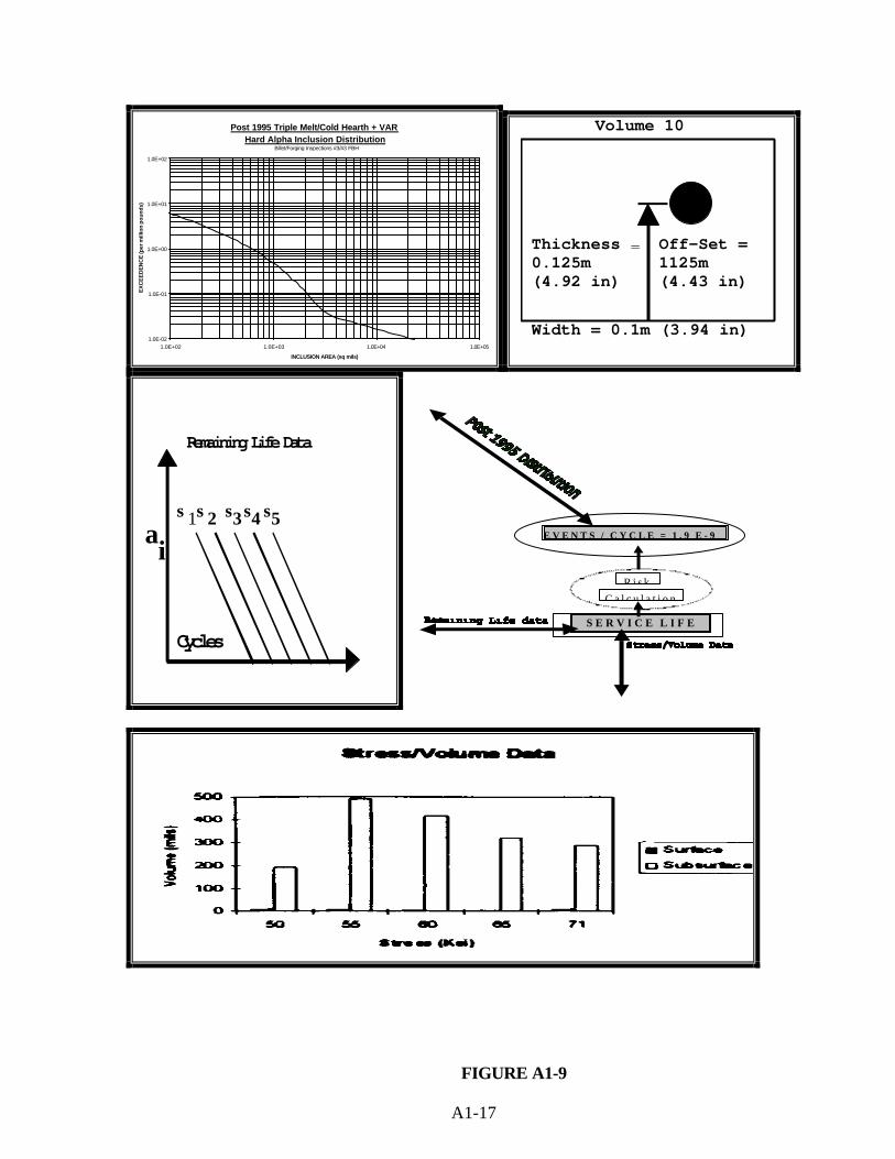
a. Anomaly distribution curve. The anomaly distributions are provided in Appendix 3. For this test case we will use the anomaly distribution presented in FIGURE A3-7 of Appendix 3 titled “Post 1995 Triple Melt Hard-Alpha Distribution with #3 FBH billet inspection and #3 FBH forging inspection”. Billet and forging manufacturing inspections are fully accounted for in this curve. No additional modifications are necessary.

(1) It is assumed that anomalies are spherically shaped and uniformly distributed throughout the part.

(2) The anomaly distribution should be linearly extrapolated when anomaly sizes are required outside the range of data provided. The curve is shown in FIGURE A1-11.

b. POD. The POD curve used to determine the effect of an in-service inspection is contained in Appendix 5. The default curve to be used is the mean POD for ultrasonic inspection of field components, with reject indications equal to or greater than those from a 3/64 inch (1.19 mm) diameter FBH. For the test case, it is assumed that this curve applies to the whole volume, including the near surface volume of the component.

c. Maintenance exposure interval. It should be assumed that 100-percent of the fleet is ultrasonically inspected at 10,000 cycles, which represents 50-percent of the certified part life (20,000 cycles).

A1-1

d. Incubation. No anomaly incubation life should be assumed.

e. Stress. The limiting operational principal stress is the hoop stress.

f. Material Data. Two sets of material data are provided:

(1) Physical properties. Data required:

Density: 4,450 kg/m3 or 0.161 lb./in3

Young modulus: 120,000 MPa or 17.4E3 ksi Poisson's ratio: 0.361

(2) Crack Growth. Assume the following data represents both air and vacuum crack propagation. Crack propagation rate:

da/dN = 9.25 E-13 (DK)3.87 (da/dN in m/cycle and D K in MPa�m)

- or

da/dN = 5.248 E-11 (DK)3.87 (da/dN in in/cycle and D K in ksi�in ) K threshold = 0.0 MPa�m or 0 ksi�in Fracture toughness = 64.5 MPa�m or 58.7 ksi�in Yield = 834 MPa or 121.0 ksi UTS = 910 MPa or 132.0 ksi

(a) The above data applies at the test case component temperature.

(b) Crack propagation data are for a stress ratio of zero, therefore, no stress ratio correction is required.

(c) These data were taken from MCIC-HB-01R, Damage Tolerant Design Handbook, A Compilation of Fracture and Crack Growth Data for High Stress Alloys, vol. 1, dated December 1983 (page 411.257, Figure 4.113.104). It represents generic Ti 6-4 Paris fit data. These data are provided for example purposes only, and do not constitute a recommendation for analyzing actual components.

3. Test Case Analysis Guidelines

a. Analytical guidelines for the probabilistic assessments are provided with the intent to minimize the variations of the applicants results due to analytical assumptions.

The practice presented is based on a typical embedded anomaly probabilistic fracture-mechanics approach. The component is subdivided into zones, the relative risk or probability of fracture (POF) is calculated for each zone, and results for each zone summed statistically to arrive at the total component POF or relative risk.

(1) This analytical approach can be broken down into five basic steps:

(a) Stress analysis.

(b) Zone definition and volume calculation.

(c) Crack growth model definition.

(d) Crack growth calculation.

(e) Zone and total part POF calculation.

(f) Paragraph 4 of this Appendix provides a systematic example for the calibration test case.

b. General Analytical Guidelines:

(1) Stress Analysis. The level of mesh refinement of the part model is left up to the individual applicant’s discretion. However, steps should be taken to ensure that the final answer does not change by a significant amount (5-percent on relative risk or POF) if a finer mesh is chosen.

(2) Zone Definition. Zones are defined as regions of the component (typically made up of a number of finite elements) where life is approximately constant for a given initial crack size. Grouping elements into zones based on stress intervals of 5

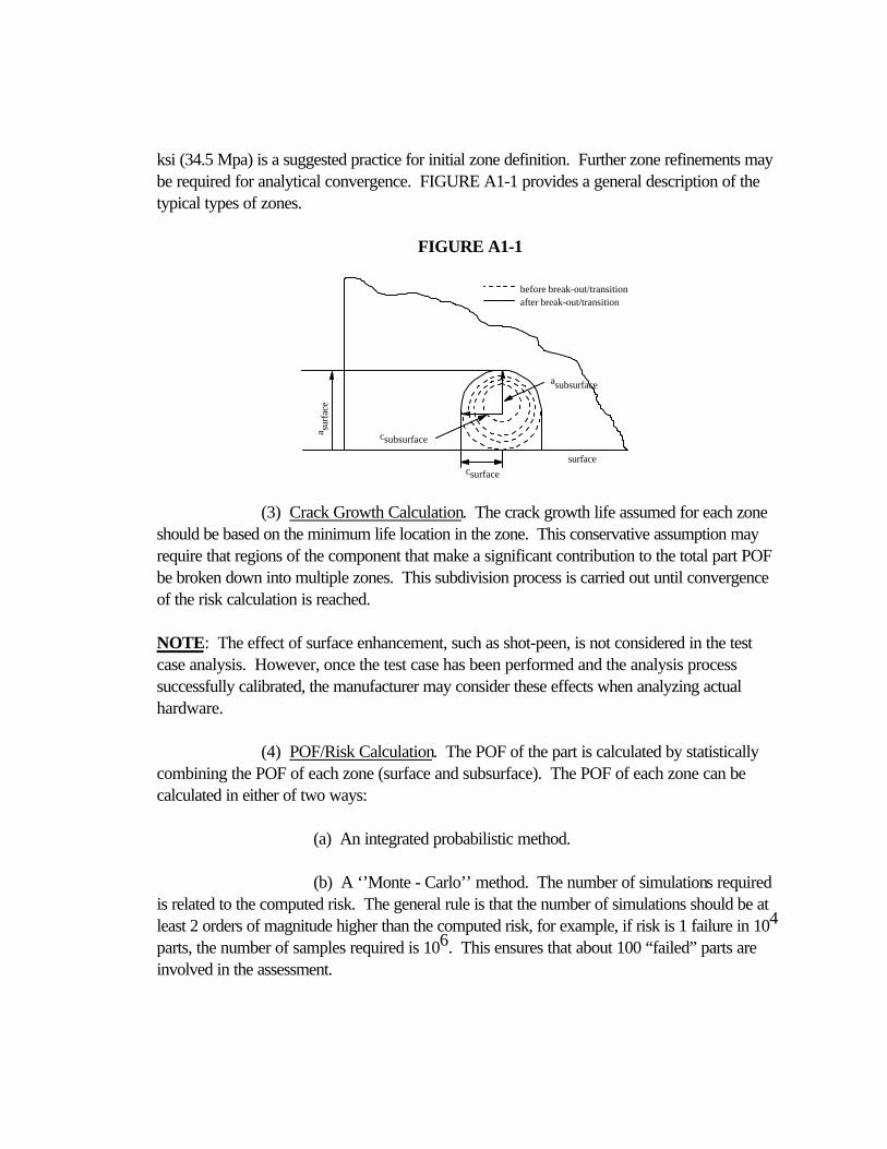
ksi (34.5 Mpa) is a suggested practice for initial zone definition. Further zone refinements may be required for analytical convergence. FIGURE A1-1 provides a general description of the typical types of zones.

FIGURE A1-1

surface

subsurfacea

subsurfacec

surf

ace

a

before break-out/transition after break-out/transition

surfacec

(3) Crack Growth Calculation. The crack growth life assumed for each zone should be based on the minimum life location in the zone. This conservative assumption may require that regions of the component that make a significant contribution to the total part POF be broken down into multiple zones. This subdivision process is carried out until convergence of the risk calculation is reached.

NOTE: The effect of surface enhancement, such as shot-peen, is not considered in the test case analysis. However, once the test case has been performed and the analysis process successfully calibrated, the manufacturer may consider these effects when analyzing actual hardware.

(4) POF/Risk Calculation. The POF of the part is calculated by statistically combining the POF of each zone (surface and subsurface). The POF of each zone can be calculated in either of two ways:

(a) An integrated probabilistic method.

(b) A ‘’Monte - Carlo’’ method. The number of simulations required is related to the computed risk. The general rule is that the number of simulations should be at least 2 orders of magnitude higher than the computed risk, for example, if risk is 1 failure in 104

parts, the number of samples required is 106. This ensures that about 100 “failed” parts are involved in the assessment.

c. Specific Guidelines for Fracture-Mechanics Modeling, Zone Definition, and Volume Calculations:

(1) Subsurface Zones.

(a) Surface enhancements must not be modeled for the test case, however, they should be considered when analyzing actual components.

(b) The maximum principal stress in each zone should be used in the crack growth calculations.

(c) The impact of stress gradients should be considered. To reach a converged solution, high stress near surface regions of the part may require additional refinement beyond the 5 ksi bands suggested in the general guidelines (e.g., disk bores and bore sides). Subdivision of these regions into subsurface "onion skin" layers, like the surface volumes discussed next, will likely capture the rapid change in life from surface to subsurface and reduce conservatism in the prediction. Engineering judgement and experimentation will be required to determine the optimum near surface zone geometry (i.e., width and thickness).

(d) A surface crack growth correction factor should be considered in the stress intensity (K) solution for cracks transitioning to surface cracks.

(e) The crack should be positioned at the life limiting location in each zone.

(f) A circular crack geometry (a = c) should be assumed.

(g) The defect area should be considered equal to the area of the circular crack.

(h) The zone volume should be assumed to be equal to the volume of the finite elements (or fractions of elements) used to construct the zone.

(i) When transitioning to a surface crack, the crack depth (a) should be taken as the diameter of the subsurface crack (2a) just as it touches the surface (see FIGURE A1-2).

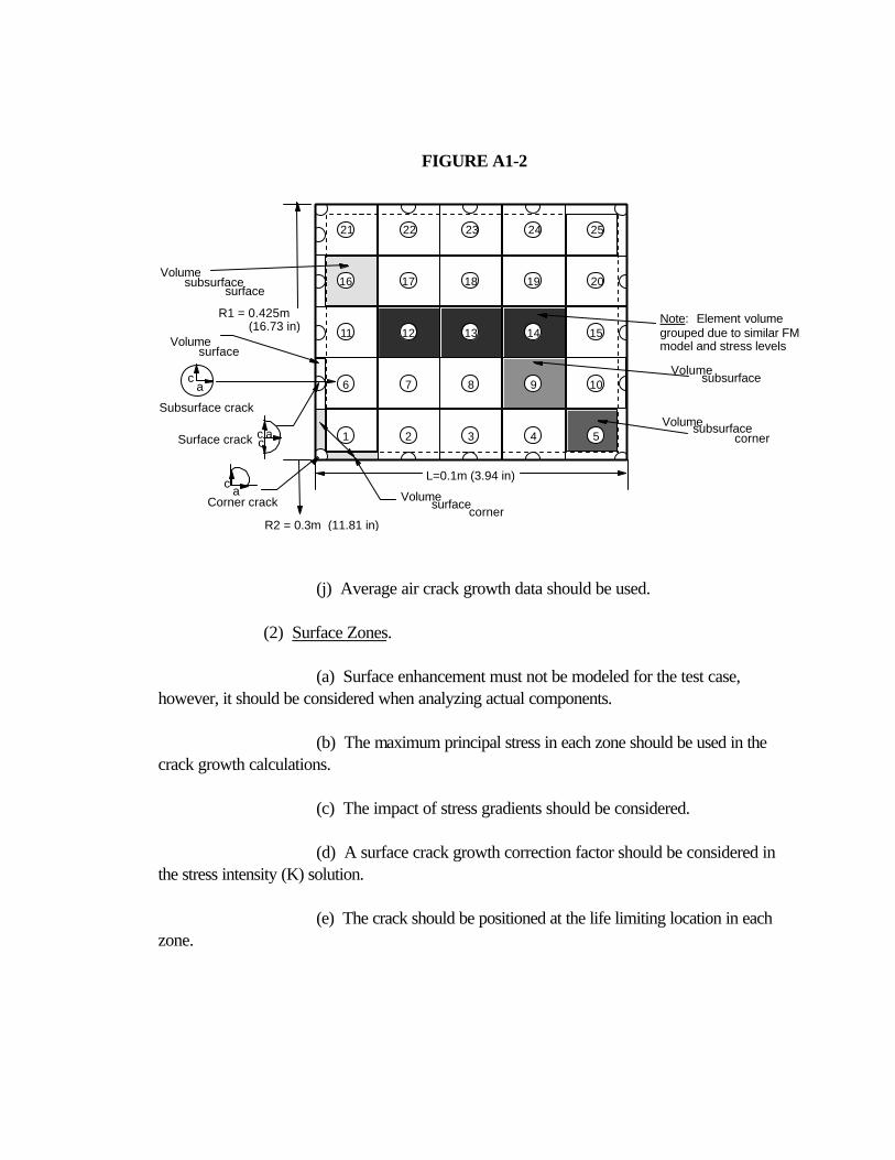
FIGURE A1-2

Note:

21 22 23 24 25

16 17 18 19 20

11 12 13 14 15

6 7 8 9 10

1 2 3 4 5

R1 = 0.425m (16.73 in)

Volume

Volume

Volume surface

Volume subsurface

surface

Subsurface crack

c a

ac c

Corner crack a

c Volume

surface corner

L=0.1m (3.94 in)

Surface crack

Element volume grouped due to similar FM model and stress levels

subsurface

subsurface corner

R2 = 0.3m (11.81 in)

(j) Average air crack growth data should be used.

(2) Surface Zones.

(a) Surface enhancement must not be modeled for the test case, however, it should be considered when analyzing actual components.


(c) The impact of stress gradients should be considered.

(d) A surface crack growth correction factor should be considered in the stress intensity (K) solution.


(f) A 2:1 crack aspect ratio should be assumed, with surface length (2c) equal to twice the depth (a).

(g) The defect area should be assumed equal to 1/2 the area of a circle with a radius of crack depth (a).

(h) The volume should be based on the zone surface face length and an onion skin thickness of 0.020 in (0.5 mm).

(i) Average air crack growth data should be used.

(3) Surface Corner Zones.

(a) Surface enhancements must not be modeled for the test case, however, should be considered when analyzing actual components.


(c) The impact of stress gradients should be considered.

(d) A surface crack growth correction factor should be considered in the stress intensity (K) solution.


(f) A 1:1 crack aspect ratio should be assumed, with surface length (c) equal to depth (a).

(g) The defect area should be assumed equal to 1/4 the area of a circle with the radius of crack depth (a).

(h) The volume should be based on the zone surface face lengths and an onion skin thickness of 0.020 in (0.5 mm).

(i) Average air crack growth data should be used.

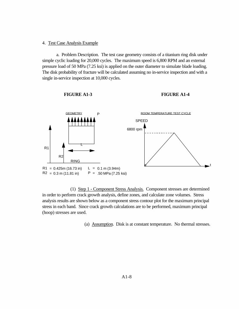
4. Test Case Analysis Example

a. Problem Description. The test case geometry consists of a titanium ring disk under simple cyclic loading for 20,000 cycles. The maximum speed is 6,800 RPM and an external pressure load of 50 MPa (7.25 ksi) is applied on the outer diameter to simulate blade loading. The disk probability of fracture will be calculated assuming no in-service inspection and with a single in-service inspection at 10,000 cycles.

FIGURE A1-3 FIGURE A1-4

GEOMETRY ROOM TEMPERATURE TEST CYCLEP

L

R2

R1

RING

0.425m (16.73 in) 0.3 m (11.81 in)

= =

R1 R2

0.1 m (3.94m) .50 MPa (7.25 ksi)

= =

L P

SPEED

6800 rpm

o t

(1) Step 1 - Component Stress Analysis. Component stresses are determined in order to perform crack growth analysis, define zones, and calculate zone volumes. Stress analysis results are shown below as a component stress contour plot for the maximum principal stress in each band. Since crack growth calculations are to be performed, maximum principal (hoop) stresses are used.

(a) Assumption. Disk is at constant temperature. No thermal stresses.

A1-8

FIGURE A1-5

Rim 400.0 MPa (58 ksi)

434.4 MPa (63 ksi)

468.9 MPa (68 ksi)

503.4 MPa (73 ksi)

537.9 MPa (78 ksi)

572.4 MPa (83 ksi) Bore

NOTE: Typically a Kt would be applied to the rim stress due to the dovetail slot. However, it has not been included in the test case.

(2) Step 2 - Stress Volume Calculation. Incremental volumes are used to determine the probability of having an anomaly in a particular region of the part. The disk is partitioned into zones, where within a zone the residual life is nearly constant. Next, the volume of each zone is calculated. The disk shown in FIGURE A1-6 has been partitioned in to 36 zones. Guidelines for defining the volume of each zone are provided in paragraph 3 of this Appendix. Stress volume results are shown in Table A1-1 of this Appendix.

(a) Assumptions:

1. Stress volumes partitioned at 5 ksi (34.5 MPa) increments are good starting points to perform the risk integration.

2. A 0.020 in (0.5-mm) thick onion skin provides adequate definition of the surface volumes.

A1-9

Component Stress Model Component Principal Stress Contour Plot

Further breakup of the highstress/low lifezones to reach

FIGURE A1-6

Component Stress Model Stress Volume Definition

0.020 in (0.5 mm) Onion Skin

9

15.2e

15.2c

15.2a

15.2d

15.2b

10

15.315.1

14.2

13. 2

12.2

11

14.3

13.3

12.312.1

13. 1

14.1

171

2 18

3 19

204

convergence

Further break up of the high stress/low life zones performed to reach convergence

21

22

5

6

7 23

8 24 16

A1-10

Table A1-1: Zone Volume Data

Zone Number Volume

1 0.69 cm3 (0.042 in3) 2 18.8 cm3 (1.15 in3) 3 34.9 cm3 (2.13 in3) 4 29.2 cm3 (1.78 in3) 5 24.2 cm3 (1.48 in3) 6 20.1 cm3 (1.23 in3) 7 16.1 cm3 (0.98 in3) 8 0.49 cm3 (0.030 in3)9 134.37 cm3(8.20 in3)

10 3675.5 cm3(224.29 in3) 11 6809.8 cm3(415.56 in3)

12.1 144.48 cm3(8.81 in3) 12.2 5403.46 cm3(329.68 in3) 12.3 144.48 cm3(8.81 in3) 13.1 119.95 cm3(7.32 in3) 13.2 4488.2 cm3(273.84 in3) 13.3 119.95 cm3(7.32 in3) 14.1 99.58 cm3(6.08 in3) 14.2 3724.1 cm3(227.22 in3) 14.3 99.58 cm3(6.08 in3) 15.1 79.82 cm3(4.87 in3)

15.2a 1958.8 cm3(119.51 in3) 15.2b 324.02 cm3(19.77 in3) 15.2c 459.58 cm3(28.04 in3) 15.2d 182.75 cm3(11.15 in3) 15.2e 91.13 cm3(5.56 in3) 15.3 79.82 cm3(4.87 in3)

16 94.90 cm3(5.79 in3) 17 0.69 cm3(0.042 in3) 18 18.8 cm3(1.15 in3) 19 34.9 cm3(2.13 in3) 20 29.2 cm3(1.78 in3) 21 24.2 cm3(1.48 in3) 22 20.1 cm3(1.23 in3) 23 16.1 cm3(0.98 in3) 24 0.49 cm3(0.030 in3)

A1-11

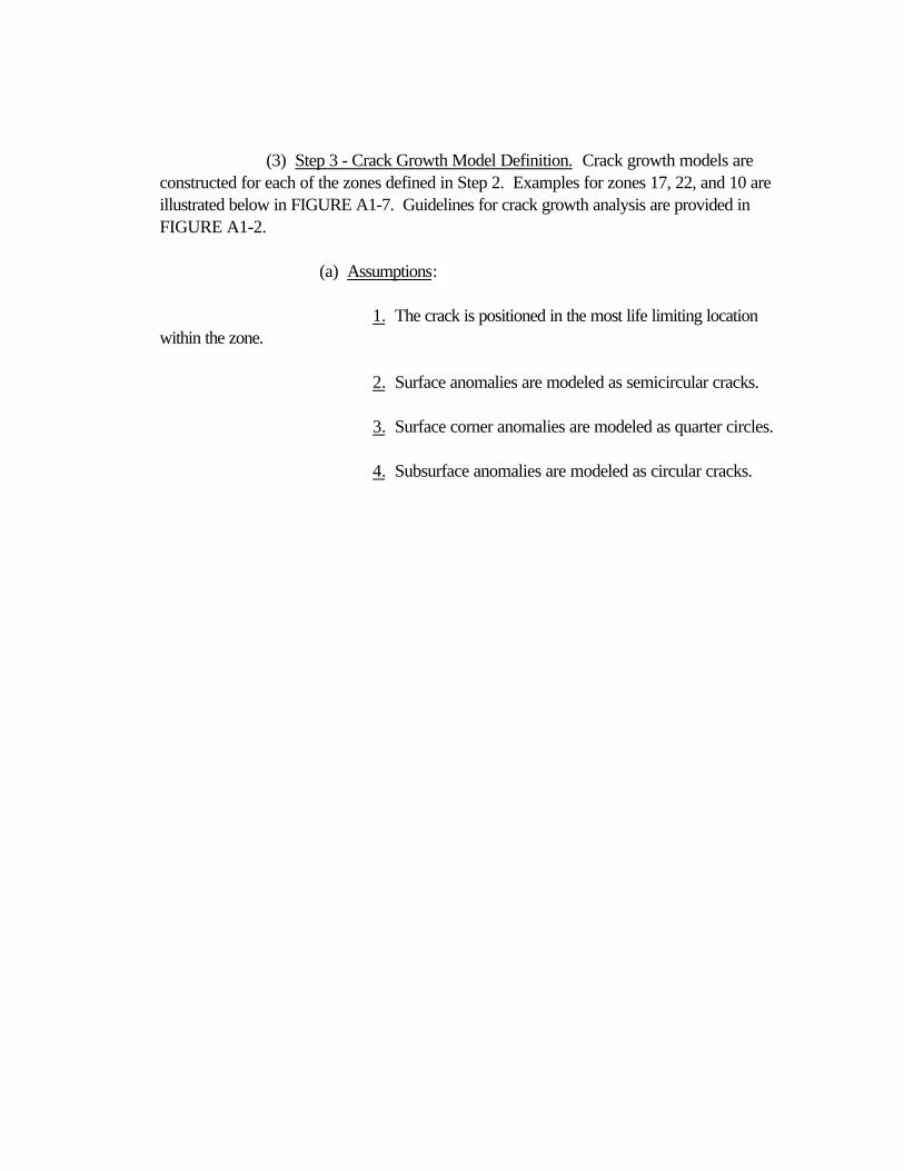
(3) Step 3 - Crack Growth Model Definition. Crack growth models are constructed for each of the zones defined in Step 2. Examples for zones 17, 22, and 10 are illustrated below in FIGURE A1-7. Guidelines for crack growth analysis are provided in FIGURE A1-2.

(a) Assumptions:

1. The crack is positioned in the most life limiting location within the zone.

2. Surface anomalies are modeled as semicircular cracks.

3. Surface corner anomalies are modeled as quarter circles.

4. Subsurface anomalies are modeled as circular cracks.

W i d t h = 0 . 1 m ( 3 . 9 4 i n . ) T

hickness = 0.125 m (4.92 in.)

W i d t h = 0 . 1 m ( 3 . 9 4 i n . )

Thickness = 0.125 m

(4.92 in.)

Off

set =

0.1

125

m (

4.43

in.)

Z o n e 1 0

Z o n e 2 2

Z o n e 1 7

T h i c k n e s s = 0 . 1 m ( 3 . 9 4 i n . )

Wid

th =

0.0

376

m (1

.48

in.)

FIGURE A1-7: Zone Crack Location

A1-13

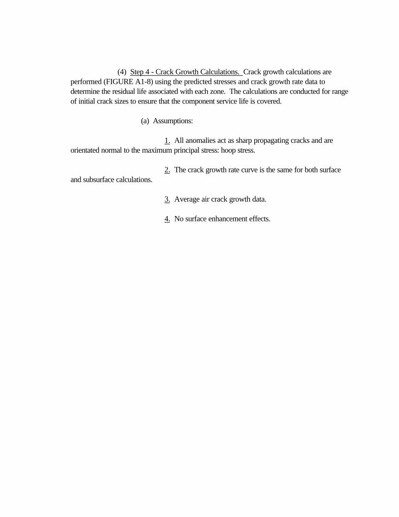
(4) Step 4 - Crack Growth Calculations. Crack growth calculations are performed (FIGURE A1-8) using the predicted stresses and crack growth rate data to determine the residual life associated with each zone. The calculations are conducted for range of initial crack sizes to ensure that the component service life is covered.

(a) Assumptions:

1. All anomalies act as sharp propagating cracks and are orientated normal to the maximum principal stress: hoop stress.

2. The crack growth rate curve is the same for both surface and subsurface calculations.

3. Average air crack growth data.

4. No surface enhancement effects.

FIGURE A1-8

Crack Growth Data

80

0

10

20

30

40

50

60

70

0 1 2 Time

Str

ess

(ksi

)

Volume Stress Cycles

Remaining Life Data

a i

Volume No.

Cycles

A1-15

(5) Step 5 - Relative Risk Calculation – No In-Service Inspection. The probability of fracture for each stress volume is calculated integrating the volume, anomaly distribution, and residual life information from the previous steps (FIGURE A1-9). The results for each zone are statistically summed to determine the total component probability of fracture. The calculated probability of fracture without an in-service inspection is 1.9 E - 09 events/cycle.

A1-16

Post 1995 Triple Melt/Cold Hearth + VAR Hard Alpha Inclusion Distribution

1.0E-02

1.0E-01

1.0E+00

1.0E+01

1.0E+02

1.0E+02 1.0E+03 1.0E+04 1.0E+05

INCLUSION AREA (sq mils)

EX

CE

ED

EN

CE

(per

mill

ion

poun

ds)

Billet/Forging Inspections #3/#3 FBH

Width = 0.1m (3.94 in)

Thickness = 0.125m (4.92 in)

Volume 10

Off-Set = 1125m (4.43 in)

Remaining Life Data

ai

Cycles

s1s2 s3s4 s5

R i s k C a l c u l a t i o n

S E R V I C E L I F E

E V E N T S / C Y C L E = 1 . 9 E - 9

FIGURE A1-9

A1-17

(6) Step 6 - Relative Risk Calculations – With a Single In-Service Inspection. The “with inspection” probability of fracture calculations are performed in the same manner as in step 5, except the ultrasonic technique (UT) inspection POD data and cycles to inspection are included in the risk integration (FIGURE A1-10). The calculated probability of fracture with a mid-life inspection is 1.4 E - 09 events/cycle.

(a) Assumptions:

1. The UT inspection POD curve is applicable for 100-percent of the component volume (surface connected and subsurface).

2. Inspection performed at 10,000 cycles.

3. Assume the anomaly area in the inspection plane is equivalent to the anomaly area in the stress plane.

A1-18

P o s t 1 9 9 5 T r i p l e M e l t / C o l d H e a r t h + V A R

H a r d A l p h a I n c l u s i o n D i s t r i b u t i o n

B i l l e t / F o r g i n g I n s p e c t i o n s # 3 / # 3

Risk

Calculation Service Life

Events/Cycle = 1.4 E-9

Remaining Life Data

ai

Cycles

Inspection POD

FIGURE A1-10

A1-19

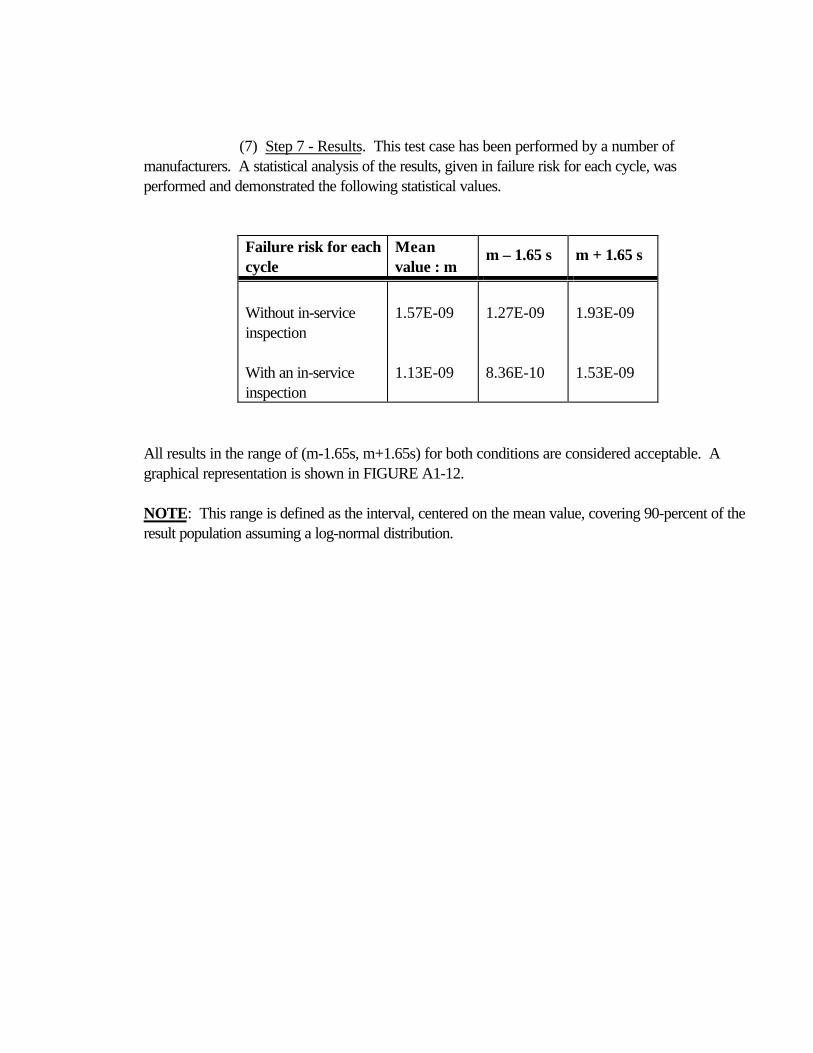
(7) Step 7 - Results. This test case has been performed by a number of manufacturers. A statistical analysis of the results, given in failure risk for each cycle, was performed and demonstrated the following statistical values.

Failure risk for each cycle

Mean value : m

m – 1.65 s m + 1.65 s

Without in-service inspection

With an in-service inspection

1.57E-09

1.13E-09

1.27E-09

8.36E-10

1.93E-09

1.53E-09

All results in the range of (m-1.65s, m+1.65s) for both conditions are considered acceptable. A graphical representation is shown in FIGURE A1-12.

NOTE: This range is defined as the interval, centered on the mean value, covering 90-percent of the result population assuming a log-normal distribution.

FIGURE A1-11



1.0E+02 1.0E+03 1.0E+04 1.0E+05

INCLUSION AREA (sq mils)

1.0E-02

1.0E-01

1.0E+00

1.0E+01

1.0E+02

EX

CE

ED

EN

CE

(p

er m

illio

n p

ou

nd

s)

A1-21

FIGURE A1-12: Results

m - 1.65 sm - 1.65 s = 1.27E-09 TOTAL FAILURE RISK

WITHOUT INSPECTION

MEAN VALUE m = 1.57E-09

m - 1.65 s = 1.27E-09 m + 1.65 s = 1.93E-09

1.0E-10 1.0E-09 1.0E-08

FAILURE RISK PER CYCLE

TOTAL FAILURE RISK

WITH AN IN-SERVICE INSPECTION

MEAN VALUE m = 1.13E-09

m - 1.65 s = 8.36E-10 m + 1.65 s = 1.53E-09

1.0E-10 1.0E-09 1.0E-08

FAILURE RISK PER CYCLE

APPENDIX 2

SOFT TIME INSPECTION EXAMPLE

1. This Appendix provides an example of an acceptable process for setting the opportunity inspection requirements that will be specified in Airworthiness Limitations Section of the Instructions for Continued Airworthiness. As discussed in Section 4, the application of the opportunity inspection is one of a number of options available to reduce the predicted POF in the event that a component design does not meet the DTR criteria.

a. Section 4 introduced the following three scenarios for opportunity inspections to clarify the actions that could be taken at a maintenance opportunity. They are (1) Hardware available for opportunity inspection, (2) Module below soft time interval, (3) Module above soft time interval. Examples of the first and third scenarios will be presented in this Appendix, and the second scenario would be analyzed in a similar fashion to the third scenario.

b. Key elements in determining opportunity inspection requirements given any scenario are the type of inspection method and associated level of sensitivity, the maintenance interval at which the hardware will be exposed for inspection, and the cyclic threshold or soft time interval for module exposure at which time the inspections will be invoked. Given a scenario, details of an inspection plan can take many forms. FIGURE A2-1 shows the decision process for selecting the appropriate inspection requirements. This flowchart will be referenced throughout this section to guide the discussion.

A2-1

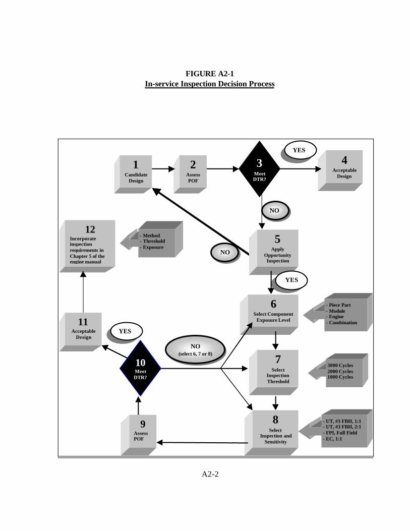
FIGURE A2-1 In-service Inspection Decision Process

1 Candidate

Design

2 Assess POF

3 Meet DTR?

4 Acceptable

Design

5 Apply

Opportunity Inspection

6 Select Component

Exposure Level

7 Select

Inspection Threshold

8 Select

Inspection and Sensitivity

- Piece Part - Module - Engine - Combination

3000 Cycles 2000 Cycles 1000 Cycles

- UT, #3 FBH, 1:1 - UT, #3 FBH, 2:1 - FPI, Full Field - EC, 1:1

9 Assess POF

12 Incorporate inspection requirements in Chapter 5 of the engine manual

11 Acceptable

Design

YES

NO

YES

NO

YES

10 Meet DTR?

NO (select 6, 7 or 8)

- Method - Threshold - Exposure

A2-2

2. Example of Scenario (1), Hardware Available for Opportunity Inspection.

a. It was shown in Appendix 1 that the predicted POF for the simple ring disk, without the benefit of in-service inspection is 1.9 E-09 events/cycle (Block 2 of FIGURE A2-1). Therefore, the ring disk design does not meet the 1.0 E-09 event/cycle DTR (A “No” answer at Block 3). If the ring disk POF was less than the DTR, the design would be considered acceptable (Block 4) and no in-service inspection would be required.

b. Assuming a design change is not possible (for example, a reduction in stress, change in material, or enhance manufacturing inspection), the decision is made (Block 5) to explore the opportunity inspection option to reduce the component risk below the DTR.

c. With the decision made to pursue the inspection route, the level of maintenance opportunity is selected for study. The options available are piece part, module, engine, or some combination of these opportunities. The desire is to select an exposure level or combination of levels that minimizes the impact on the operator, yet has a high potential of reducing the component risk level. It is anticipated that the applicant will use trial and error to arrive at the optimum solution. However, working with this damage tolerance criteria will give the applicant experience for making good initial selections reducing the amount of analytical effort in future analyses. For the initial pass, a one time ultrasonic inspection (UT) at first piece part exposure (Block 6), and an inspection threshold of zero cycles (Block 7) will be evaluated. The piece part maintenance exposure distribution for the ring disk is shown in FIGURE A2-2 below.

FIGURE A2-2

R i n g D i s k O v e r h a u l F i r s t P i e c e P a r t E x p o s u r e D i s t r i b u t i o n

1 2 0

1 0 0

8 0

6 0

4 0

2 0

0 0 5 0 0 0 1 0 0 0 0 1 5 0 0 0 2 0 0 0 0 2 5 0 0 0

C y c l e s

Mean = 9000 Cycles Standard Deviation = 1500

A2-3

d. A UT inspection rejecting indications equal to or greater than a number 3 FBH is selected. The solid line in Appendix 5, FIGURE A5-4 is the POD for this inspection (Block 8).

e. The probability of fracture calculations are performed (Block 9) in the same manner as in step 6 of Appendix 1, except instead of a fixed inspection at 10,000 cycles, inspections are assumed to occur as the piece parts are exposed. The piece part exposure distribution is treated as a random variable in the probabilistic analysis.

f. The calculated probability of fracture is 1.3 E-9 events/cycle, still greater than the DTR (A “No” answer at Block 10). On a second pass a more sensitive UT inspection is assumed, rejecting indications equal to or greater than ½ the response from a number 3 FBH. The associated POD for this inspection is represented by the dotted line in FIGURE A5-5. The resulting POF is 9.9 E-10 events/cycle, meeting the DTR (A “Yes” answer at Block 10).

g. The design would be considered acceptable (relative to damage tolerance criteria) and the following inspection requirements would be placed in Airworthiness Limitations Section of the Instructions for Continued Airworthiness (Step 12):

(1) Inspect at first piece part exposure.

(2) UT inspection calibrated to a #3 FBH.

(3) Reject indications equal to or greater than ½ the response from a number 3 FBH calibration.

(4) Include reference to detailed UT inspection procedures.

2. Example of Scenario (3), Module Above Soft Time Interval

a. For this example, exposure of the ring disk piece parts is expected to occur at a lower rate than in the previous scenario. This change is depicted in FIGURE A2-3 below.

A2-4

FIGURE A2-3: New Ring Disk First Part Exposure Distribution

100

80

60

40

20

0 0 5000 10000 15000 20000 25000

Cycles

Mean = 19000 Cycles Standard Deviation = 7000 Cycles

b. The predicted POF, assuming this new exposure distribution, and the same UT inspection and sensitivity as in scenario (1), is 1.2E-09 events/cycle. Since the predicted POF exceeds the DTR, additional action is warranted.

c. Assuming that it is not reasonable to use a more sensitive UT field inspection (for example, calibration to a smaller flat bottom hole), the module exposure distribution is evaluated (see FIGURE A2-4 below).

FIGURE A2-4: New Ring Disk First Exposure Distributions

120

100

80

60

40

20

0

Module Exposure

Piece Part Exposure

0 5000 10000 15000 20000 25000 Cycles

Piece Part Exposure (Mean = 19000, Std = 7000)

Module Exposure (Mean = 13000 , Std = 3000 )

d. The resulting predicted POF is 8.3 E-10 events/cycle, clearing the DTR with margin. However, specifying UT inspection of the ring disk at module exposure requires that the disk be removed from the module increasing the burden on the operator. Since there is margin between the predicted POF and the DTR, an alternative inspection plan

will be considered that will alleviate some of the burden of forcing modules to piece part level. This approach implements the soft time inspection interval scenario. Instead of going to just the module exposure, the inspections would be performed at piece part exposure for a specified cyclic interval, then change to inspections at module exposure. The cyclic interval before imposing inspection based on module exposure is the soft time inspection interval.

FIGURE A2-5

Combination of First Piece part and Module Exposure Distributions

120 100 80 60 40 20 0

Module Composite

Piece Part

0 5000 10000 15000 20000 25000

Cycles

e. This strategy essentially accelerates the piece part exposure rate as shown in FIGURE A2-5. By iterating on the length of the soft time interval, a 12,300 cycle value is found to yield a POF of 1.0 E-09 events for each cycle, satisfying the DTR criteria. The design would be considered acceptable relative to damage tolerance criteria and the following inspection requirements would be placed in the Airworthiness Limitations Section of the Instructions for Continued Airworthiness (Step 12):

(1) Inspect at first piece part exposure.

(2) For parts not previously inspected before 12,300 cycles, inspect at first module exposure above 12,300 cycles, soft time inspection interval.

(3) UT inspection calibrated to a #3 FBH.

(4) Reject indications equal to or greater than ½ the response from a number 3 FBH calibration.

(5) Include reference to detailed UT inspection procedures.

f. The information provided in this section is for example only. Each individual component design and engine maintenance practice may require different solutions than those presented here. The key is that Airworthiness Limitations Section of the Instructions for Continued Airworthiness requirements should reflect actions consistent with the analytical assumptions made to meet the DTR criteria.

APPENDIX 3

DEFAULT ANOMALY DISTRIBUTION CURVES

1. Anomaly Distribution Curves

a. The anomaly distribution curves associated with hard-alpha inclusions in titanium engine rotors are illustrated in this Appendix (FIGURES A3-1 - A3-18). The following text provides additional information associated with the use of these distributions.

(1) The distributions are applicable only to hard-alpha inclusions in rotor grade (premium) titanium melted after 1995 using triple VAR or CHM plus VAR processes.

(2) It is crucial to use the appropriate distribution curve that accurately reflects the inspection sensitivities performed at the billet and forging stages of the manufacturing process.

(3) For example, the material must be inspected using UT to at least a #3 FBH with the reject level set at one half that of the calibration level. See Appendix 5 for additional instructions. Inspections must be performed at both the billet and sonic shape stages.

(4) The distribution accounts for all steps required to manufacture a finished part, including the in-process billet and sonic shape forging ultrasonic inspections. Therefore, the distribution used should reflect the inspection sensitivities used in the billet and forging inspections, and should not be altered.

(5) Referring to the FIGURES in this Appendix:

(a) The vertical axis represents the expected number of hard-alpha inclusions for each million pounds of titanium. This information should be treated as the probability of having an inclusion of a given size or larger (exceedance probability).

(6) The horizontal axis is the inclusion cross-sectional area including the hard-alpha core and the surrounding diffusion zone. A circular inclusion cross section should be assumed with the corresponding diameter used as the initial size in the crack growth analysis.

A3-1

FIGURE A3-1


Billet / Forging Inspections #5/#3 FBH

0.1

0.01 100 1000 10000 100000

DEFECT INSPECTION AREA (sq mils)

100

10

1

A3-2

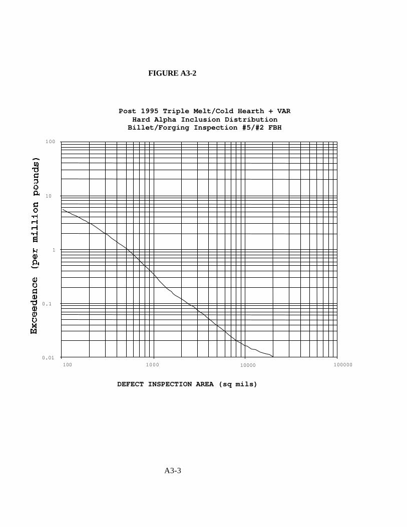
10

FIGURE A3-2


Billet/Forging Inspection #5/#2 FBH

100

1

0.1

0.01 100 1000 10000 100000


A3-3

10

1

FIGURE A3-3



100

0.1

0.01 100 1000 10000 100000


A3-4

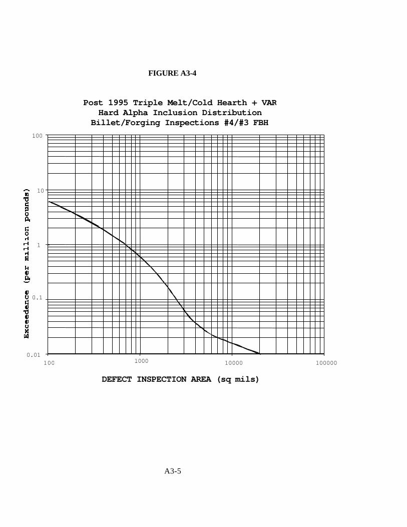
FIGURE A3-4



0.1

0.01 1000100 10000 100000


100

10

1

A3-5

FIGURE A3-5



100

10

1

0.1

0.01 100 10000 1000001000


A3-6

1

FIGURE A3-6



100

10

0.1

0.01 100 1000 10000 100000


A3-7

FIGURE A3-7


Billet/Forging Inspections #3/#3 FBH 100

10

1

0.1

0.01 100 1000 10000 100000


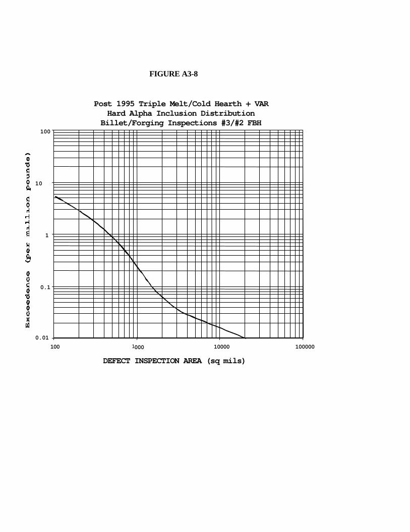
10

FIGURE A3-8



1

0.1

0.01 100 1000 10000 100000


FIGURE A3-9



10

1

0.1

0.01 100 1000 10000 100000


A3-10

FIGURE A3-10



10

1

0.1

0.01 100 1000 10000 100000


A3-11

1

FIGURE A3-11


Billet/Forging Inspections #2/#2 FBH100

10

0.1

0.01 100 1000 1000 10000

0 0 DEFECT INSPECTION AREA (sq mils)

A3-12

10

FIGURE A3-12

Post 1995 Triple Melt/Cold Hearth + VAR Hard Alpha Inclusion Distribution Billet/Forging Inspections #2/#1

100

1

0.1

0.01 100 1000 10000 100000


FIGURE A3-13


Billet/Forging Inspections MZ (12-13" billet)/#3 FBH 100

10

1

0.1

0.01 100 1000 10000 100000


1

FIGURE A3-14


Billet / Forging Inspections MZ (12-13" Billet)/#2 FBH

100

10

0.1

0.01 100 1000 10000 100000


A3-15

FIGURE A3-15


Billet / Forging Inspections MZ (12-13" Billet)/#1 FBH 100

10

1

0.1

0.01 100 1000 10000 100000


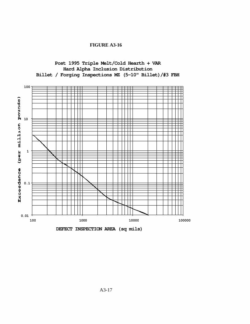
FIGURE A3-16



100

10

1

0.1

0.01 100 1000 10000 100000


A3-17

FIGURE A3-17



100

10

1

0.1

0.01 100 1000 10000010000


FIGURE A3-18



100

10

1

0.1

0.01 1000 10000 100000100


A3-19

APPENDIX 4

DEFAULT POD APPLICABILITY

1. Use of Default POD Data

a. This Appendix defines conditions relevant to the use of accepted estimates of the probability of detection (POD) for specific types of anomalies and specific nondestructive evaluation/inspection techniques, which may be considered as default values when applied under appropriately similar conditions. The conditions defined in this Appendix do not necessarily guarantee the validity of these POD values. For example, if inspection parameters, such as penetrant concentration or temperature, are inadequately controlled, the penetrant capability shown in the accompanying graph will not be attained, even if the correct penetrant is selected. Use of a written plan for controlling and monitoring inspection processes is recommended (see paragraph 3 of this Appendix).

b. If the conditions described for each inspection are not satisfied, the resultant inspection capability and reliability will be reduced. Accordingly, the use of the default POD values would then be inappropriate and would result in an overly optimistic damage tolerance assessment.

2. Demonstrations of Inspection Capability

a. For ECI and ultrasonic inspection techniques, alternative default POD curves are given. Choice of the appropriate POD curve must be based on demonstration that the stated calibration and reject signal levels are attainable on the component being inspected, and, for example, not prevented by noise or geometrical features. The demonstration conditions should be appropriate to the properties of the part inspected that may affect the inspectability, such as surface conditions, depth to be inspected, proximity to edges, etc. No other demonstration of these default capabilities is necessary, as long as the requirements for the specific inspection technique are satisfied (see paragraphs 3-6 of this Appendix).

b. It should be noted that, for specific inspection techniques applied under well controlled conditions, it may be possible to achieve POD values that are significantly better than the default POD values. Advantage may be taken of any such improved capability and reliability only if it is supported by a well documented demonstration

A4-1

program. Similarly, a well documented demonstration program may be necessary in order to measure POD values appropriate to specific conditions that are excluded from those the default values is supported by explicit, reasonable assumptions.

3. General Restrictions and Applicability

a. The inspection process must be well controlled, and performed in accordance with acceptable procedures, such as those defined by the engine standard practices manual, and consistent with good industrial inspection practices, such as those defined by MIL-STD’s, or equivalent industry standards.

b. Pertinent inspection process parameters such as coverage, probe indexing, and scanning speeds (see paragraph 4 of Section 3, and paragraphs 4-6 of this Appendix), should be governed by written procedures;. Inspection plans and any inspection fixturing, should be designed to minimize human and other sources of variability.

c. Inspectors must be fully qualified and trained for each MIL-STD-410, ASNT-TC-1A, ATA-105, or equivalent, and provided with adequate training instructions in the specific inspection method.

d. The default POD data presented in this AC are applicable only to titanium alloys used for engine disks, and only to inspected material. Geometrical conditions, such as radii and edges can create areas where inspections can not be accomplished. Limitations also exist relative to depth of penetration and near surface resolution. Conditions under which the default POD data were acquired are outlined in paragraphs 4-6 of this Appendix; advice about the equivalence of alternative conditions should be sought from those with expertise in NDE. Areas of high compressive residual stress can have negative effects on the capability of various NDE techniques, most notably penetrant inspection.

e. Applicability of the default POD data is limited to components exhibiting no abnormal surface conditions, and that have been properly cleaned for each shop manual requirements. No other special pre-inspection cleaning or polishing is required.

4. Restrictions and Applicability: ECI

a. The ECI is an inspection technique suitable for the detection of surface or near-surface anomalies. For the purposes of this document, it is intended primarily for application to engine-run components. The default POD data were acquired under the following conditions:

(1) Probes containing absolute coils, with inspection frequency in the range 2-6 MHz.

(2) Probe fixturing capable of following surface contours of the component being inspected, with adequate control of attitude, lift-off and scan indexing. The scan direction was parallel with any uniform feature changes.

(3) Provision was made for automatic recording of the inspection process signals or automated alarm, or both, when the inspection threshold is exceeded.

b. The default POD data apply to surface-connected low-cycle fatigue cracks. Cracks are assumed to have a 2-to-1 aspect (length:depth) ratio. Crack sizes are expressed in terms of the length at the surface. Cracks must not be obscured by oxide, contaminants, etc. Inspected surfaces should be flat, or only moderately curved. Choice of the appropriate POD curve from those provided must be based on component demonstration of the attainable inspection sensitivity (see paragraph 2 of this Appendix).

5. Restrictions and Applicability: Penetrant Inspection (PT/FPI)

a. PT is an inspection technique suitable for the detection of anomalies that are open to the inspected surface. For the purposes of this document, it is intended primarily for application to engine-run components. The default POD data were acquired under the following conditions:

(1) Fluorescent penetrants qualified as level 4 by MIL-I-25135, or equivalent, and used with dry powder developer (as a minimum).

(2) Application of penetrant and developer was automated, or for each standard practices; (see, for example, MIL-STD-6866 and AMS-2847).

A4-3

(3) Manipulation of the part was possible to present to the inspector an unimpeded view of the surface to be inspected.

b. The default POD data apply to surface-connected low-cycle fatigue cracks. Cracks are assumed to have a 2-to-1 aspect (length:depth) ratio. Crack sizes are expressed in terms of the length at the surface. Cracks must not be obscured by oxide, contaminants, etc. Inspected surfaces should readily visible. Choice of the appropriate POD curve from those provided must be based on whether focused or full field inspection conditions apply, as those terms are defined in paragraph 3 in the main body of the AC.

6. Restrictions and Applicability: Ultrasonic Inspection (UT)

a. UT is an inspection technique suitable for the detection of subsurface anomalies. For the purposes of this document, it is intended for application both to billets and to engine-run components. The default POD data were acquired under the following conditions:

(1) 5 MHz inspection frequency.

(2) Water immersion inspection conditions.

(3) Normal incidence longitudinal wave mode for inspection of billet using single 0.5 inch x 1.0 inch cylindrically focused transducer.

(4) Shear wave mode for inspection of finish-machined components using 0.75 inch diameter spherically focused transducer.

(5) Transducer (search unit) fixturing was capable of following surface contours of the component being inspected, with adequate control of attitude and scan indexing.

(6) Provision was made for automatic recording of the inspection process signals or automated alarm, or both, when the inspection threshold was exceeded.

b. For ultrasonic inspection, the default POD data apply to mixtures of anomalies typical of those that may be found in billet, or in engine-run material, as appropriate. These anomalies include hard-alpha associated voids or cracks, strain induced porosity,

etc. It should be noted that other anomaly types may occur, such as high density inclusions, but these are not included in the current analysis. Anomaly sizes are expressed in terms of maximum cross-sectional area perpendicular to the sound beam, including associated diffusion zones where appropriate.

c. Inspected finish-machined surfaces should be flat, or only moderately curved. Billets should be circular-cylindrical, and in customary pre-inspection conditions (turned, ground, or peeled).

d. Choice of the appropriate POD curve from those provided must be based on component demonstration of the attainable inspection sensitivity (see paragraph 2 of this Appendix). Provision must be made to maintain this sensitivity at all depths, and effective distance-amplitude compensation is required.

APPENDIX 5

DEFAULT POD CURVES

60

50

40

FIGURE A5-1

POD FOR FLUORESCENT PENETRANT INSPECTION OF FINISH-MACHINED SURFACES

100

90

80

70

30

20

10

0 10 100 1000

ANOMALY LENGTH (mils)

Full-field inspection Applicability: Directed inspection

MIL-I-25135 Level 4 penetrants with dry powder developer (as minimum)

A5-2

FIGURE A5-2

MEAN (50% CONFIDENCE) POD FOR ULTRASONIC INSPECTION OF FIELD COMPONENTS

#1 FBH (1/64 INCH DIA.) CALIBRATION

0

10

20

30

40

50

60

70

80

90

100

100 1000 10000 100000

ANOMALY AREA (mils^2)

Billet: data taken with 0.5x1" cylindrically focused transducer

Finish-machined part: data taken with 0.75" diameter spherically focused transducer

Reject indications equal to or greater than those from a 1/64 in dia FBH

Reject indications equal to or greater than one half those from a 1/64 in dia FBH

Applicability:

Hard-alpha associated inclusions/ cracks/voids (includes diffusion zones)

Billet: 5MHz longitudinal (compressional) wave inspection

circular-cylinderical billet

Finish-machined: 5MHz shear (transverse) wave inspection

applicable only if the indicated sensitivity is attainable

A5-3

FIGURE A5-3


#2 FBH (2/64 INCH DIA.) CALIBRATION 100

90

80

70

60

50

40

30

20

10

0 1000 10000 100000100






Applicability:

Hard-alpha associated inclusions/ cracks/ voids (includes diffusion zones)

Billet: 5MHz longitudinal (compressional) wave inspection circular-cylinderical billet

Finish-machined: 5MHz shear (transverse) wave inspection

Applicable only if the indicated sensitivity is attainable

A5-4

FIGURE A5-4


#3 FBH (3/64 INCH DIA.) CALIBRATION

0

10

20

30

40

50

60

70

80

90

100

100 1000 10000 100000






Applicability:

Hard-alpha associated inclusions/ cracks/ voids (includes diffusion zones)

Billet: 5MHz longitudinal (compressional) wave inspection

circular-cylinderical billet

Finish-machined: 5MHz shear (transverse) wave inspection applicable only if the indicated sensitivity is attainable

A5-5

FIGURE A5-5

MEAN (50% CONFIDENCE) POD FOR EDDY CURRENT OF FINISH-MACHINED SURFACES

100

90

80

70

60

50

40

30

20

10

0 10 100

ANOMALY LENGTH (mils)

Reject at the calibration notch threshold Applicabilty:response and above

Absolute coils, 2-6 MHz inspection frequency Reject at one half the calibration notch threshold response and above Calibration on 0.030" x 0.015" notch applicable

only if the indicated sensitivity is attainable

A5-6

subject: date: ac no: engine rotors initiated by: … · 1/8/01 . ac no: engine rotors . initiated...

Documents