sub-pixel edge localization based on laser waveform analysis · sub-pixel edge localization based...

SUB-PIXEL EDGE LOCALIZATION BASED ON LASER WAVEFORM ANALYSIS B. Jutzi a, J. Neulist a, U. Stilla b

a FGAN-FOM Research Institute for Optronics and Pattern Recognition, 76275 Ettlingen, Germany - {jutzi,neulist}@fom.fgan.de

b Photogrammetry and Remote Sensing, Technische Universitaet Muenchen, 80290 Muenchen, Germany - [email protected]

Commission III, Working Group III/3

KEY WORDS: Urban, Analysis, Laser scanning, LIDAR, Edge, Sub-pixel precision.

ABSTRACT:

Laser range data is of high interest in photogrammetry. However, compared to passive imagery, it usually has a lower image resolution, making geometry extraction and modeling challenging. A method to overcome this handicap using a laser scanner capable of full waveform analysis is proposed. The recorded pulse waveform is analyzed to find range and intensity values for all of the surfaces in the beam footprint. Sub-pixel edge localization is implemented and tested for straight edges of man-made objects, allowing a much higher precision of geometry extraction in urban areas. The results show that it is possible to find edges with an accuracy of at least one tenth of a pixel.

1. INTRODUCTION

The automatic generation of 3-d models for a description of man-made objects, like buildings, is of great interest in photogrammetric research. In photogrammetry, a spatial surface is classically measured by triangulation of corresponding image points from two or more pictures of the surface. The points are manually chosen or automatically detected by analyzing image structures. Besides this indirect measurement using object characteristics dependant on natural illumination, active laser scanner systems allow a direct and illumination-independent measurement of range. Laser scanners capture the range of 3-d objects in a fast, contactless and accurate way. Overviews for laser scanning systems are given in (Huising & Pereira, 1998; Wehr & Lohr, 1999; Baltsavias, 1999).

For the task of automatic model generation, a precise measurement of the edges and vertices of regularly shaped objects is paramount. Often, the spatial resolution of laser scanners used in urban surveying is not sufficient for this. In this case, an approach to locate the edges with sub-pixel accuracy is desirable. To achieve this, as much information as possible should be gained per pixel1 to offset the low number of pixels in the image.

Current pulsed laser scanner systems for topographic mapping are based on time-of-flight ranging techniques to determine the range of the illuminated object. The signal analysis to determine the elapsed time between the emitted and backscattered laser pulses typically operates by analogous threshold detection. Some systems capture multiple reflections caused by objects which are smaller than the footprint located in different ranges. Such systems usually record the first and the last backscattered laser pulse (Baltsavias, 1999).

First pulse as well as last pulse exploitation is used for different applications like urban planning or forestry surveying. While first pulse registration is the optimum choice to measure the hull of partially penetrable objects (e.g. canopy of trees), last pulse registration should be chosen to measure non-penetrable surfaces (e.g. ground surface). Due to multiple pulse reflection at the boundary of buildings and the processing by first or last 1 Note that in this paper the label pixel describes the conical region in space illuminated by a single laser beam. During visualization, this region is compressed into a single pixel of a displayed image, hence the name.

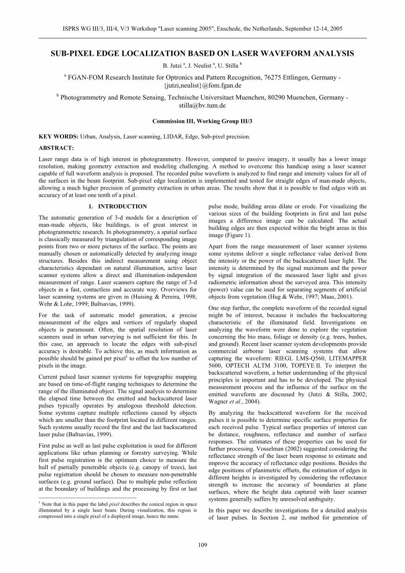
pulse mode, building areas dilate or erode. For visualizing the various sizes of the building footprints in first and last pulse images a difference image can be calculated. The actual building edges are then expected within the bright areas in this image (Figure 1).

Apart from the range measurement of laser scanner systems some systems deliver a single reflectance value derived from the intensity or the power of the backscattered laser light. The intensity is determined by the signal maximum and the power by signal integration of the measured laser light and gives radiometric information about the surveyed area. This intensity (power) value can be used for separating segments of artificial objects from vegetation (Hug & Wehr, 1997; Maas, 2001).

One step further, the complete waveform of the recorded signal might be of interest, because it includes the backscattering characteristic of the illuminated field. Investigations on analyzing the waveform were done to explore the vegetation concerning the bio mass, foliage or density (e.g. trees, bushes, and ground). Recent laser scanner system developments provide commercial airborne laser scanning systems that allow capturing the waveform: RIEGL LMS-Q560, LITEMAPPER 5600, OPTECH ALTM 3100, TOPEYE II. To interpret the backscattered waveform, a better understanding of the physical principles is important and has to be developed. The physical measurement process and the influence of the surface on the emitted waveform are discussed by (Jutzi & Stilla, 2002; Wagner et al., 2004).

By analyzing the backscattered waveform for the received pulses it is possible to determine specific surface properties for each received pulse. Typical surface properties of interest can be distance, roughness, reflectance and number of surface responses. The estimates of these properties can be used for further processing. Vosselman (2002) suggested considering the reflectance strength of the laser beam response to estimate and improve the accuracy of reflectance edge positions. Besides the edge positions of planimetric offsets, the estimation of edges in different heights is investigated by considering the reflectance strength to increase the accuracy of boundaries at plane surfaces, where the height data captured with laser scanner systems generally suffers by unresolved ambiguity.

In this paper we describe investigations for a detailed analysis of laser pulses. In Section 2, our method for generation of

ISPRS WG III/3, III/4, V/3 Workshop "Laser scanning 2005", Enschede, the Netherlands, September 12-14, 2005

109

synthetic test data is discussed. A description of the generalwaveform analysis, image segmentation and surface boundaryextraction can be found in Section 3. The actual sub-pixel edge localization algorithms are developed in Section 4. Section 5 presents results and a discussion of the merits and flaws of themethod.

2. DATA GENERATION

To simulate the temporal waveform of the backscattered pulses a scene model (i) and a sensor model (ii) is required (Jutzi & Stilla, 2004).

2.1

2.1.1

2.1.2

2.2

2.2.1

2.2.2

2.2.3

2.2.4

3.1

Scene modeling

Scene representation

For a 3-d scene representation, our simulation setup considers geometric and radiometric features of the illuminated surface inthe form of a 3-d object model with homogeneous surfacereflectance.

Sampling

The object model with homogeneous surface reflectance is then sampled at a higher spatial resolution than the scanning grid we simulate and process, to enable us to simulate the spatial distribution of the laser beam. Considering the position andorientation of the sensor system we receive high-resolutionrange and intensity images (45-fold oversampling, i.e. oneimage pixel is produced by averaging over 45x45 high-resolution sub-pixels. The oversampling window size does nothave any practical relevance if it is sufficiently large to not induce errors in a higher magnitude as those incurred by ourdiscretized beam profile). Depending on the predetermined position and orientation of the sensor system, various range images can be captured.

Sensor modeling

a b

c dFigure 1. Sections of an urban scene (Test area Karlsruhe,

Germany).a) elevation images captured by first pulse mode,b) elevation images captured by last pulse mode, c) difference image of first and last pulse mode, d) section of the difference image (building boundary).

The sensor modeling takes into account the specific properties of the sensing process: the position and orientation of the sensor, the laser pulse description, scanning and the receiverproperties.

Orientation

To simulate varying perspectives, a description of the extrinsic orientation of the laser scanning system with the help of aGPS/INS system is used.

Laser pulse description

The transmitted laser pulse of the system is characterized byspecific pulse properties (Jutzi et al., 2002). We assume a Gaussian pulse energy distribution in both space and time, the spatial distribution thus being radially symmetric. With realdata, the sampled actual pulse distribution depending on the used laser type can be used to model the edge appearance in theimage (q.v. Section 4.1).

Scanning

Depending on the scan pattern of the laser scanner system, the grid spacing of the scanning, and the divergence of the laserbeam, a sub-area of the high-resolution range image is processed. By convolving this sub-area with the temporal waveform of the laser pulse, we receive a high-resolutionintensity cube. Furthermore, the corresponding sub-area of thehigh-resolution intensity image is weighted with the spatial energy distribution of the laser beam, where the grid spacing istaken to be 6 of the spatial beam energy distribution (i.e. the grid lines are at ±3 relative to the beam center) to take intoaccount the amount of backscattered laser light for each reflectance value. Then we have a description of thebackscattered laser beam with a higher spatial resolution than necessary for processing.

Receiver

By focusing the beam with its specific properties on the detector of the receiver, the spatial resolution is reduced and this is simulated with a spatial undersampling of the sub-areas.

Finally we receive an intensity cube spaced with the scanningwidth of the simulated laser scanner system and containing the temporal description of the backscattered signal. Because eachintensity value in the sub-area is processed by undersampling, multiple reflections can be observed in the backscattered signal.

3. DATA ANALYSIS

Algorithms are developed and evaluated with simulated signals of synthetic objects. First, a signal preprocessing of the intensity cube with a matched filter is implemented to improvethe detection rate. These results are used to analyze the waveform of each pulse for gaining the surface properties:range, reflectance and number of peaks. Then the surfaceproperties are processed with a region based segmentationalgorithm. By the use of images the region boundary pixelsderived from multiple reflections at the same spatial positionare shared by separate regions.

Pulse property extraction

Depending on the size of the observed surface geometry in relation to the laser beam (footprint and wavelength) different properties can be extracted (Jutzi & Stilla, 2003). In this paperwe focus on the pulse properties average time value, maximumintensity and number of peaks.


110

The average time value is processed to determine thedistance from the system to the illuminated surface.

The maximum intensity value is computed to get adescription for the reflectance strength of the illuminatedarea.

Multiple peaks in one signal indicate multiple surfaces at differing ranges illuminated by the beam. Therefore, theyare clues to object boundaries.

For determining the property values for each pulse of the wholewaveform the intensity cube is processed in different ways.First, the pulse has to be detected in the signal profile by using a matched filter. Then, a neighborhood area of interest in the temporal waveform is selected for temporal signal analysis.

For obtaining surface characteristics, each waveform of thecube is analyzed for pulse property values. For pulse detection it is necessary to separate each single pulse from thebackground noise. The number of detected pulses depends critically on this separation method. Therefore the signalbackground noise is estimated, and where the intensity of the waveform is above three times the noise standard deviation for a duration of at least 5 ns (full-width-half-maximum of the pulse), a pulse is assumed to have been found and a waveform interval including the pulse is accepted for further processing.

Typical surface features we wish to extract from a waveformare range, roughness, and reflectance. The corresponding pulseproperties of these surface features are: time, width and intensity. Because of the strong fluctuations of the waveform,extracting the relevant properties of the waveform can bedifficult. Therefore, the recorded waveform is approximated bya Gaussian to get a parametric description. Fitting a Gaussian to the complete waveform instead of quantizing a single value of the waveform has the advantage of decreasing the influence of noise and fluctuation. To solve the Gaussian mixture problem, the Gauss-Newton method (Hartley & Zisserman, 2000) with iterative parameter estimation is used. The estimated parametersfor pulse properties are the averaged time value , standard deviation and maximum intensity a:

2

22

( )exp( )22

( ) a tw t (1)

To start the iteration, we use the actual parameter values (timeat pulse maximum, width of signal at half pulse height, and pulse maximum) of the original waveform.

The averaged time value of the estimated waveform is used to exploit the temporal form of the received pulses. The averagedrange value r can then easily be determined by

2cr (2)

where c is the speed of light.

3.24.1

Segmentation

General approaches for segmenting laser range data, as those described by Besl (1988), usually do not take into account theadditional information acquired by full waveform processing and therefore have to be expanded upon.

By using waveform processing, we are not only generating a range image, but in fact a whole set of data for each pixel. Forthe purposes of this paper, the features of particular importance

will be: range for each return pulse, intensity for each returnpulse, and number of return pulses. The number of return pulses is used as a clue to region boundaries, while range and intensityfurther facilitate identifying homogeneous regions inside these boundaries. Without these multiple pulse clues, the regionboundaries can not reliably be pinpointed with pixel accuracy.Since the sub-pixel localization scheme works on the intensityof pixels partially covering a surface, this pixel precision isnecessary for the accuracy of the resulting edges.

Proceeding from these boundary clues, an iterative regiongrowing algorithm examines the range properties of all pulsesin the spatial neighborhood: if the range difference of a pulseand the proofing pulse is below a given threshold, then the pulse is connected and grouped as a new element to this region.

The segmentation leads to a description of image pixels as region interior or region boundary. The region interior is characterized by single reflections and fills up the region to theboundary. For each homogeneous region found in this manner,the average return pulse power P0 inside this region is calculated and stored. The region boundary pixels are connected in a 4-neighbor fashion, i.e. each boundary pixel has at least one neighbor in horizontal or vertical direction which also belongs to the boundary.

4. BOUNDARY REFINEMENT

To achieve a higher precision for object localization andreconstruction, it is desirable to further refine thesemeasurements (Figure 2a). Standard sub-pixel edge localization approaches use the intensity of grayscale images to obtain improved edge information. The intensity values acquired mayform a grayscale image and thus permit the application of thesealgorithms to our data. But we will go one step further since thefull waveform laser data has several advantages over passiveoptical images for this purpose.

For precise edge localization, it is important to know the properties of the data acquisition unit very well and be able to model the effects of a beam being only partially reflected by a given surface. This modeling will be explained in the firstsubsection. In the second subsection, we will show how this model enables us to determine the sub-pixel location of an edgein each pixel. The third subsection will examine astraightforward approach to determine edge direction using neighborhood information. Then we will detail our proposed scheme to use the complete edge information to fortify the edgeestimate in the fourth subsection. The last subsection will deal with vertices and the problem of their precise localization in theimage.

For the purposes of this paper, we will call the measured edge pixels of the image boundary pixels, or corners, if they do notbelong to a straight edge. Furthermore, let the true geometry be denoted by edges and vertices, to clear up the description of our approach.

Modeling the rasterized edge intensity profile

As shown in the introduction to this Section, it is necessary tobe aware of the meaning of the intensity values acquired alongside the range measurements. Therefore we will examinethe results of a beam hitting a homogeneous surfaceperpendicular to the beam propagation direction assuminguniform reflectance for the surface.

An analysis of the spatial beam profile (Jutzi et al., 2002) has shown that it can be approximated by a radially symmetric


111

B

B

O

O

B B

O

B

I

1

3

2

B

B

O

O

B B

O

B

I

B

B

O

O

B B

O

B

I

1

3

21

3

2

B

B

O

O

B B

O

B

I

1

3

2

B

B

O

O

B B

O

B

I

B

B

O

O

B B

O

B

I1

3

2

B

B

O

O

B B

O

B

I

4

1

3

2

B

B

O

O

B B

O

B

I

B

B

O

O

B B

O

B

I

4

2

B

B

O

O

B B

O

B

I2

B

B

O

O

B B

O

B

I

B

B

O

O

B B

O

B

I

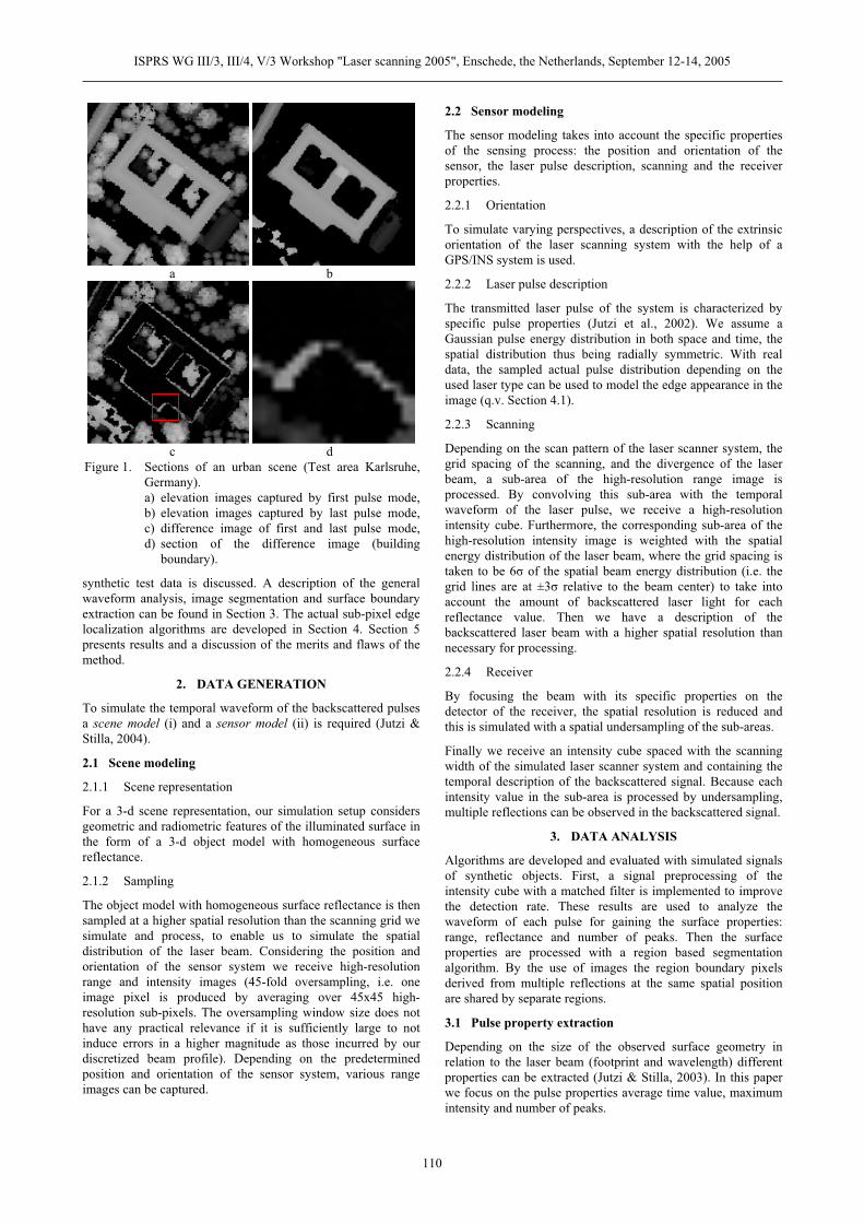
a b c d Figure 2. Edge estimation (Pixels labelled I are inner region pixels, O are outside pixels, and B are boundary pixels):

a) sample of edges 1, 2 and 3, b) estimated edges by considering the distance from the beam center d,c) possible edges tangential to two circles, d) final edge by using the signs of di

Gaussian distribution for the sake of simplicity. For the case of the beam partially hitting the surface, we assume the objectedge to be straight. In reality, this is not a very strong demand,since the edge has to be essentially straight only for the extent of the beam. Furthermore, we let the edge be parallel to the y-coordinate axis. Because of the radial symmetry of the beamprofile, the results can then be generalized to arbitrary edge orientations. If we let d the distance of the surface edge to thebeam center, the standard deviation of the beam profile and P0the average beam power inside the region (q.v. Section 3.2), wefind the reflected beam power to be

2 2 2

2 2

2 2( )

x y xd do o

BP PP d e dx dy e dx (3)

This integral can be described by the complementary error function

( ) ( )2o

BPP d erfc d (4)

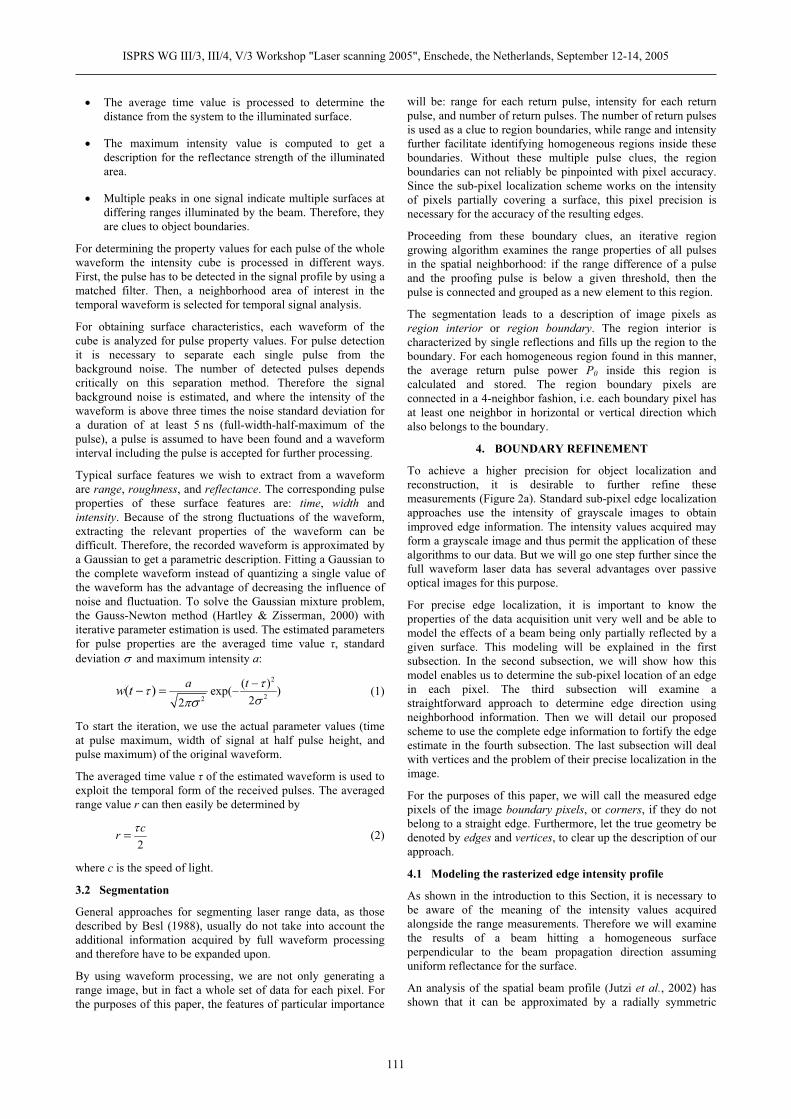
Figure 3a shows a plot of the beam intensity versus the edge offset. Here, the grid spacing is 2f and the standard deviation of the Gaussian used to model the beam profile is f/3.

4.2

4.3 4.4

Sub-pixel edge localization in each pixel

Looking at a boundary pixel, we can easily acquire the edge distance from the beam center dS by inverting the above relationship (using standard numerical procedures) and applying it to the measured return pulse power PB. However, itis impossible to estimate the edge orientation using only asingle pixel (Figure 2b). Therefore we now have a circle with radius dS around the beam center and know that the edge has tobe a tangent to this circle (Figure 3b).

To determine the orientation of this tangent, and along with itthe orientation of the edge, we have to use neighborhoodinformation to further restrict the edge hypotheses.

Estimating tangents in 2 neighborhood edge pixels

A very simple approach consists of using a neighborhood boundary pixel to reduce the problem’s degrees of freedom. If we have hints that both of these pixels belong to the samestraight object edge, we can use their combined information toestimate the edge. We are looking for a line that is tangential to two circles (radii d1 and d2, respectively). This problemgenerally has four different solutions (Figure 2c),mathematically. From the intensity response, we know which side of the beam center the tangent passes through, since we

actually get a signed result for d1 and d2, corresponding to the measured intensity being smaller or larger than 50% of the intensity inside the region (Figure 3a & b). If the signs of these two radii are different, the correct edge solution is one of thetwo tangents crossing between the circles, else one of the outer tangents.

From the segmentation step it is already known which side isthe inner and which is the outer side of the boundary, i.e. we know where the boundary is connected to the region. Again,watching the signs of d1 and d2, we know which of the two remaining solutions to choose (Figure 2d, in this case both of the signs are negative).

However, this straightforward approach is very sensitive tonoisy data, since it does not use an over-determined system of equations. We will be applying our method to urban areas,where we assume much longer edges to be present. This fulledge information can be used to gain higher precision results.

Figure 3. a) Edge with distance dS, b) Integration over the spatial beam profile (the grid spacing is 2f)

Complete edge localization

To use the complete information available for any given edge, we first have to determine the set of boundary pixels belonging to that edge. In the description of the segmentation algorithm,we already explained how to find region boundaries (Section 3.3). This boundary is transformed into a polygon, at firsttaking each pixel as a vertex (solid line in Figure 4). If there areany pixels in this list occurring more than once, all of their instances are removed. We do this because we assumed each

d

surface

P0 / 2

P0

0

dS

0f

PB (d)

a

b

PB (dS)

-f


112

pixel to belong to only one edge, therefore mixed pixels are notallowed to appear in our calculation.

This vertex list is then pruned by removing all vertices not significantly affecting the polygon contour. This is achieved bytentatively removing each vertex in turn from the contour(dashed line) and calculating the distance of the new polygon(dotted line) to all boundary pixels along this edge. If the largest of these distances g is smaller than one half pixel, the vertex isremoved permanently. This step is repeated until no morevertices can be removed.

Figure 4. Region boundary simplification

The last polygon found in this fashion is now a pixel-preciseestimate of the region boundary, composed of a minimalnumber of vertices and edges of maximal length. To increase the precision of our estimates for each of these edges, we selectthe set of all boundary pixels along this edge, leaving out the vertices themselves because of our assumption of pixels fullybelonging to straight edges.

For this set of k points,

(5) 2{1,2,3, , }( )i i kp

we calculate the edge distances di from the pixel intensity andsolve the optimization problem

2

1

1 (2

k

ii

)iJ np c dk

(6)

for the edge normal and the edge offset to the coordinate origin c.

n

As we see, the functional connection between PB and d does not appear in the formula. Therefore the above problem is a fairlystandard optimization problem. Going back to the image, if we replace each intensity value PB by the associated value d,Equation 6 corresponds to a standard edge localization problemin grayscale images. However, we now have the advantage of knowing our edge models exactly and can present a finer solution than those typically found for passive imagery.Parameterizing the edge normal n by its direction ( n = (cos ,sin )), we have a simple two-dimensional optimizationproblem, though it is nonlinear in . We solve for using the trust region approach by Coleman & Li (1996). The edge offsetto the origin c can then be estimated by

1

1ˆ ( ) :k

i ii

c np d n pk

d

4.5

(7)

which is very simple to solve.

Estimating vertices

Due to the modeling approach, our edge model is correct onlyfor straight edges and incorrect for vertices or curves. Therefore we have been explicitly leaving out corner pixels in the edgelocalization step. Do determine the vertices of the depictedgeometry, we calculate the intersections of every pair of neighboring edges.

We chose this approach since the connection of vertex location with the measured intensity is very ambiguous. Furthermore,corners are usually darker and thus more strongly affected bythe detector noise. Tying their information in to ouroptimization problem would complicate matters, remove theindependence of neighboring edge localization problems, and does not promise much gain.

5. EXPERIMENTAL VALIDATION

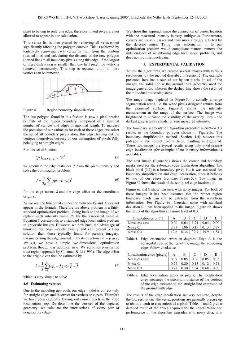
To test the algorithms, we created several images with variousresolutions, by the method described in Section 2. The examplepresented here has a size of ten by ten pixels. In all of the images, the solid line is the ground truth geometry used for image generation, whereas the dashed line shows the result of the individual processing steps.

The range image depicted in Figure 5a is actually a range segmentation result, i.e. the white pixels designate returns fromthe examined surface. Figure 5b shows the intensitymeasurement at the range of the surface. The image wasbrightened to enhance the visibility of the overlay lines – the darkest gray actually stands for zero measured intensity.

The boundary segmentation algorithm presented in Section 3.3results in the boundary polygon shown in Figure 5c. Theboundary simplification method (Section 4.4) reduces thispolygon to the correct five vertices, resulting in Figure 5d.These two images are typical results using only pixel-precise edge localization (for example, if no intensity information is available).

The next image (Figure 5e) shows the corner and boundarymasks used for the sub-pixel edge localization algorithm. The black pixel [3|2] is a boundary pixel, but it was not used forboundary simplification and edge localization, since it belongs to two of our edges (compare Figure 5c). The image in Figure 5f shows the result of the sub-pixel edge localization.

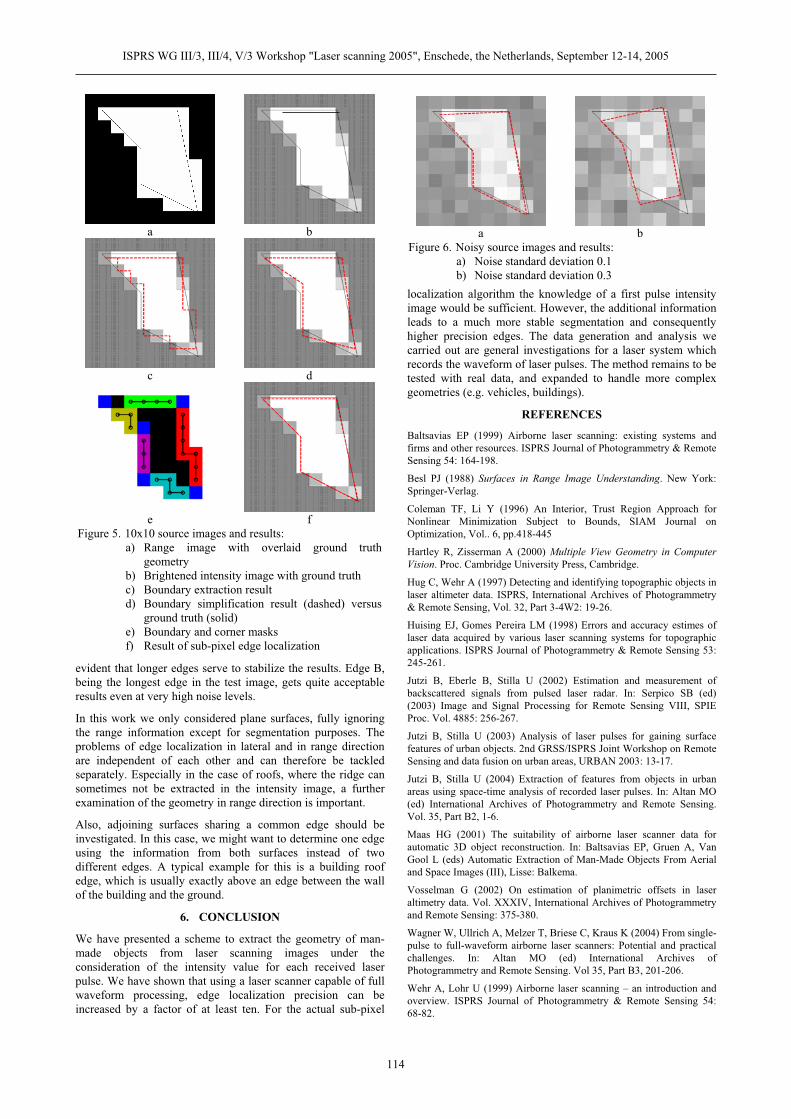
Figure 6a and b show two tests with noisy images. For both ofthese images, it has been assumed that the proper region boundary pixels can still be extracted from the waveforminformation. For Figure 6a, Gaussian noise with standarddeviation 0.1 has been applied to the image. Figure 6b shows the limits of the algorithm at a noise level of 0.3.

Orientation error [°] A B C D E Noiseless case 0.00 0.64 1.21 0.04 0.00Noise 0.1 2.33 1.86 0.19 0.13 2.77Noise 0.3 12.6 0.34 39.7 15.9 1.84

Table 1. Edge orientation errors in degrees; Edge A is thehorizontal edge at the top of the image, the remainingedges follow clockwise.

Localization error [pixels] A B C D E Noiseless case 0.09 0.05 0.06 0.05 0.03Noise 0.1 0.24 0.20 0.13 0.12 0.21Noise 0.3 0.72 0.30 1.04 0.68 0.09

Table 2. Edge localization errors in pixels; The localizationerror measures the maximum distance of the verticesof the edge estimate to the straight line extension ofthe ground truth edge.

The results of the edge localization are very accurate, despitethe low resolution. The vertex positions are generally precise up to about a tenth to a twentieth of a pixel. Tables 1 and 2 give a detailed result of the errors acquired for the edges. While theperformance of the algorithm degrades with noisy data, it is

g


113

evident that longer edges serve to stabilize the results. Edge B, being the longest edge in the test image, gets quite acceptable results even at very high noise levels.

In this work we only considered plane surfaces, fully ignoring the range information except for segmentation purposes. Theproblems of edge localization in lateral and in range direction are independent of each other and can therefore be tackledseparately. Especially in the case of roofs, where the ridge cansometimes not be extracted in the intensity image, a further examination of the geometry in range direction is important.

Also, adjoining surfaces sharing a common edge should be investigated. In this case, we might want to determine one edge using the information from both surfaces instead of twodifferent edges. A typical example for this is a building roofedge, which is usually exactly above an edge between the wall of the building and the ground.

6. CONCLUSION

We have presented a scheme to extract the geometry of man-made objects from laser scanning images under theconsideration of the intensity value for each received laserpulse. We have shown that using a laser scanner capable of fullwaveform processing, edge localization precision can be increased by a factor of at least ten. For the actual sub-pixel

localization algorithm the knowledge of a first pulse intensityimage would be sufficient. However, the additional informationleads to a much more stable segmentation and consequentlyhigher precision edges. The data generation and analysis we carried out are general investigations for a laser system which records the waveform of laser pulses. The method remains to be tested with real data, and expanded to handle more complexgeometries (e.g. vehicles, buildings).

a b

c d

e fFigure 5. 10x10 source images and results:

a) Range image with overlaid ground truthgeometry

b) Brightened intensity image with ground truth c) Boundary extraction result d) Boundary simplification result (dashed) versus

ground truth (solid) e) Boundary and corner masksf) Result of sub-pixel edge localization

a bFigure 6. Noisy source images and results:

a) Noise standard deviation 0.1 b) Noise standard deviation 0.3

REFERENCES

Baltsavias EP (1999) Airborne laser scanning: existing systems and firms and other resources. ISPRS Journal of Photogrammetry & RemoteSensing 54: 164-198.

Besl PJ (1988) Surfaces in Range Image Understanding. New York: Springer-Verlag.

Coleman TF, Li Y (1996) An Interior, Trust Region Approach forNonlinear Minimization Subject to Bounds, SIAM Journal on Optimization, Vol.. 6, pp.418-445

Hartley R, Zisserman A (2000) Multiple View Geometry in Computer Vision. Proc. Cambridge University Press, Cambridge.

Hug C, Wehr A (1997) Detecting and identifying topographic objects inlaser altimeter data. ISPRS, International Archives of Photogrammetry& Remote Sensing, Vol. 32, Part 3-4W2: 19-26.

Huising EJ, Gomes Pereira LM (1998) Errors and accuracy estimes of laser data acquired by various laser scanning systems for topographicapplications. ISPRS Journal of Photogrammetry & Remote Sensing 53: 245-261.

Jutzi B, Eberle B, Stilla U (2002) Estimation and measurement of backscattered signals from pulsed laser radar. In: Serpico SB (ed)(2003) Image and Signal Processing for Remote Sensing VIII, SPIE Proc. Vol. 4885: 256-267.

Jutzi B, Stilla U (2003) Analysis of laser pulses for gaining surface features of urban objects. 2nd GRSS/ISPRS Joint Workshop on RemoteSensing and data fusion on urban areas, URBAN 2003: 13-17.

Jutzi B, Stilla U (2004) Extraction of features from objects in urban areas using space-time analysis of recorded laser pulses. In: Altan MO (ed) International Archives of Photogrammetry and Remote Sensing.Vol. 35, Part B2, 1-6.

Maas HG (2001) The suitability of airborne laser scanner data for automatic 3D object reconstruction. In: Baltsavias EP, Gruen A, Van Gool L (eds) Automatic Extraction of Man-Made Objects From Aerialand Space Images (III), Lisse: Balkema.

Vosselman G (2002) On estimation of planimetric offsets in laseraltimetry data. Vol. XXXIV, International Archives of Photogrammetryand Remote Sensing: 375-380.

Wagner W, Ullrich A, Melzer T, Briese C, Kraus K (2004) From single-pulse to full-waveform airborne laser scanners: Potential and practical challenges. In: Altan MO (ed) International Archives of Photogrammetry and Remote Sensing. Vol 35, Part B3, 201-206.

Wehr A, Lohr U (1999) Airborne laser scanning – an introduction andoverview. ISPRS Journal of Photogrammetry & Remote Sensing 54:68-82.


114

sub-pixel edge localization based on laser waveform analysis · sub-pixel edge localization based...

Documents