study of wellbore effect on drill stem test · pdf filewilly gunary abadi, 12204003, 2nd...

STUDY OF WELLBORE EFFECT ON DRILL STEM TEST

AND IN PRODUCTION WELLS

IN ‘X’ GAS CONDENSATE FIELD

A Final Project Report

By:

WILLY GUNARY ABADI

NIM 12204003

This paper is part of the requirement to acquireBACHELOR DEGREE

In Petroleum Engineering Study ProgramFaculty of Mining and Petroleum Engineering

Bandung Institute of Technology

PROGRAM STUDI TEKNIK PERMINYAKANFAKULTAS TEKNOLOGI PERTAMBANGAN DAN PERMINYAKAN

INSTITUT TEKNOLOGI BANDUNG2008




A Final Project Report

By:

WILLY GUNARY ABADI

NIM 12204003

This paper is part of the requirement to acquireBACHELOR DEGREE

In Petroleum Engineering Study ProgramFaculty of Mining and Petroleum Engineering

Bandung Institute of Technology

Approved by:

Adviser,

Dr. Ir. Taufan Marhaendrajana

Willy Gunary Abadi, 12204003, 2nd Semester 2007/2008 1




By :

Willy Gunary Abadi*

AbstractHigh skin in the production wells can decrease the productivity index of the wells and needs high pressure drop to produce high gas rate. From Drill Stem Test (DST) analysis, It has been predicted that high skin is due to perforation in the X - field.

This skin can be caused by the high pressure overbalance when perforations, turbulent flow at near well bore (usually called non-Darcy skin), and condensate which fill into the sand face and blocks gas flow. There are different methods to capture different “skin”. Therefore, it is important to study the skin and determine strategy to mitigate that effect in the future wells.

Keywords: Drill Stem Test, non-Darcy skin, condensate blockage.

SariSkin yang tinggi pada sumur produksi dan mengurangi productivity index dari sumur dan diperlukan perbedaan tekanan yang tinggi untuk memproduksi laju alir gas yang tinggi. Dari analisa Uji Kandungan Lapisan (UKL), telah diprediksi bahwa tingginya angka yang menghalangi gas mengalir dikarenakan perforasi di lapangan-X.

Skin yang terdapat pada lapangan ini diakibatkan oleh perforasi overbalance dengan beda tekanan yang tinggi, aliran turbulen dimuka perforasi (biasa dikenal non-Darcy skin), dan kondensat yang mengisi pada muka perforasi dan mencegah aliran gas. Ada berbagai metoda untuk menentukan skin. Oleh karena itu, sangat penting untuk studi terhadap skin dan menentukan strategi yang tepat untuk mengatasi efeknya pada sumur-sumur selanjutnya.

Kata kunci: Uji Kandungan Lapisan, skin non-Darcy, penyumbatan kondensat

*Student of Petroleum Engineering ITB

2 TM-FTTM-ITB 2nd Semester 2007-2008

I. INTRODUCTION

1.1 Background

X-field is a retrograde gas reservoir. X-field location is in the Natuna sea. There are 6 appraisal wells drilled to date at X-field. Threewells have been tested after drilling, Well-2, Well-3, and Well-5. Well-2 is an exploration well tested 19 years ago. That well has 1 Drill Stem Test (DST) data at 1 perforation zone. DST at Well-2 produce some gas and condensate from abadi zone 3.

Well-3 had 5 DST at 3 perforation zones, 2 DST are additional tests performed on the same zone with either added perforations or plugging back (it mark with letter A after number in name for DST). The test zones are Gunary zone 4, Gunary zone 1 and 2, and Abadi zone 1-4. Well-5 has 3 DST that tested at 3 zones. They are Gunary zone 2, Gunary zone 1, and Abadi Zone 3. Figure 1.1 shows a cross section of X-field formation.

Fig. 1-Cross section X-field formation

Reservoir ParametersX-field is a sandstone formation with reservoir properties estimated from logging. A cut off porosity value of 8% has been assumed for estimation of net pay for DST analysis. Using this cut off, range of net porosity over tested interval is about 12% - 22% and NTG (net to gross) value is about 0.9.

Fluid ParametersAs explain before, X-field is a retrograde gas reservoir. From fluid analysis, the value of gas specific gravity range from 0.7 to 0.867 and condensate API gravity from about 51 to 59API. Gas compositional PVT analysis showsthere is no hydrogen sulfide and a few percent of carbon dioxide and nitrogen component.

1.2 Objectives

The objectives of this thesis are :• Analysis of DSTs to determine

Reservoir Characteristics (Pi, kh, skin, boundary)

• Compare DST model matching results against simulation results (kh, skin, boundary)

• Understand the effects of condensate blockage and hydraulic fracture at different rates, perms, and fluid properties.

II. DST ANALYSIS

2.1 Basic Theory

Drill Stem testDST (Drill Stem Test) is a test conducted on a drilled well completed with a temporary completion. The main objectives of DST are to help understand fluid contents of the test interval and to know reservoir characteristics such as initial pressure, permeability, skin factor, and boundaries.

DSTs usually consist of production periodsand shut in periods. There are 3 plots that can be made from DST. They are history plot, Type curve plot/log-log plot, and Horner plot/semi-log plot. History plot is the plot that shows pressure of DST gauge during the time the gauge in the well. Log-log plot is a plot of pressure and pressure derivative plot where both of X axis (time) and Y (pressure and pressure derivative) axis at logarithmic scale. Horner plot is the plot of pressure in Y axis at logarithmic scale and time at X axis at cartesian scale.

Log-log plot and Horner plot are resulted from pressure build up data when the well is shut in.

DST matching is mainly used to :1. determine formation permeability2. understand damage or stimulation

effect around the well3. determine early time range (wellbore

storage period), middle time range, and late time range effect (e.g. boundaries)

4. determined initial pressure5. determined deliverability/productivity

and AOF

Pseudo-pressure ApproachSimiliar methodology to analyses oil tests and gas tests is used. But in gas test, pseudo pressure functions were used to change pressure parameters, because the ideal gas assumption cannot be applied in many cases. This function was developed by Al-Hussainy, Ramey, and Crawford and the equation at the real pseudo pressure is :


P

Pbase

dz

Pm

2)(

Non-Darcy skinThere can be damage around the well after drilling and completions caused by drilling and completion fluids filtrate entering the formation. This various damage is lumped into a parameter called skin. If the skin value ispositive, damage occurs arround the wellbore, and if skin value negative, the well is stimulated. For high gas rates, there is another skin occurs. This skin is caused by turbulent flow (because gas rate has high velocity and low viscosity) at the sandface that yield additional pressure drop dependant upon the gas rate. It is called Non-Darcy skin because Darcy’s law assume that the flow at laminar and low velocity. This effect is greatest at near wellbore region and it is lumped into the skin effect which then becomes rate dependant i.e.

DqSS 'Where :

'S = total skinS = mechanically skin caused by damage or stimulationD = Non-darcy skin, 1/mmscfdq = gas rate, ,mmscfd

The methodology of gas well testing is directed to determine both components of the skin factor – the conventional Darcy flow component S and non-Darcy coefficient D. Since the skin effect is rate-dependent, the well must ideally be flowed at more than one rate to allow both components to be identified. Hence variable rate methods are very important in gas well testing.

2.2 Methodology

The software used to analyze the DSTs was Saphir. Data needed include pressure gauge, rate history, fluid properties, and some reservoir properties data. Fluid and reservoir data that were input to saphir are showed by table 2 and table 3 in appendix. At X-field wells, there are 9 DST data available for anaysis.

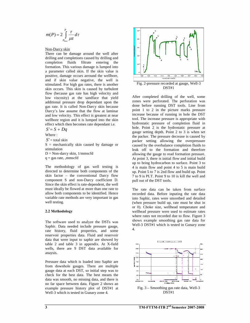
Pressure data which is loaded into Saphir are from downhole gauges. There are multiple gauge data at each DST, so initial step was to check for the best data. The best means the data was smooth, no missing data, and there is no far space between data. Figure 2 shows an example pressure history plot of DST#1 at Well-3 which is tested in Gunary zone 4.

Fig. 2-pressure recorded at gauge, Well-3 DST#1

After completed drilling of the well, some zones were perforated. The perforation was done before running DST tools. Line from point 1 to 2 in the picture marks pressure increase because of running in hole the DST tool. The increase pressure is appropriate with hydrostatic pressure of completion fluid in hole. Point 2 is the hydrostatic pressure at gauge setting depth. Point 2 to 3 is when set the packer. The pressure decrease is caused by packer setting allowing the overpressure caused by the overbalance completion fluids to leak off to the formation and therefore allowing the gauge to read formation pressure. At point 3, there is initial flow and initial build up to bring hydrocarbon to surface. Point 3 to 4 is main flow and point 4 to 5 is main build up. Point 5 to 7 is 2nd flow and build up. Point 7 to 9 is PLT. Point 9 to 10 is kill the well and pull out of the DST tools.

The rate data can be taken from surface recorded data. Before inputing the rate data into Saphir, rates were smoothed and detailed (when pressure build up, rate must be shut in or 0). Choke size, wellhead temperature and wellhead pressure were used to estimate rates where rates not recorded due to flow. Figure 3 shows example smoothing gas rate data for Well-3 DST#1 which is tested in Gunary zone 4.

Fig. 3 – Smoothing gas rate data, Well-3 DST#1


DST has some period of flowing and shut in. That can be used to build the log-log plot and Horner plot. It is relative simple to get a reservoir pressure estimate from DST if pressure build up is smooth and infinite acting at late period. The good pressure build up canalso give good log-log plot and semi-log plot.

To match the DST parameters such as kh, skin (Darcy skin and non-Darcy skin), boundaries, P, and wellbore storage constant were adjusted to match all 3 plot at the same time. Simple models infinite acting radial flow reservoir were attempted at first. By changing model and adjusting the parameters as required match could be obtained. Figure 4 until 6 shows anexample of the DST matching for Well-3 DST#1 which is tested in Gunary zone 4.

Fig. 4 – DST History plot matching, Well-3 DST#1

Fig. 5 – Log-log plot matching, Well-3 DST#1

Fig. 6 – Semi-log plot matching, Well-3 DST#1

2.3 Result

As explained above, the output of DST matching are the formation characteristic,

damage and stimulation effect, etc. All of DST Analysis basically using infinite actingmodel with boundary, homogenous reservoir, and radial flow with wellbore storage and skin at well. Most of DSTs indicated boundaries.

2.4 Discussion

The DST results shown above (e.g. k) havesome uncertainty. The first one is due to gas viscosity uncertainty. The gas viscosity was calculated from correlations and is somewhat uncertain. Viscosity value influencespermeability value because from theory DST analysis yields transmissibility which is then used to back out k. The transmissibility formula is :

kh

illitytransmisib

The second uncertainty is 2 phase behavior when flowing. If the well is flowing at pressures less than dew point pressure. Condensate may drop out from gas and causedecrease of gas saturation. Using relative permeability curves, if gas saturation decreasesrelative permeability of gas decreases and atthe same time relative permeability of oil increase. Changing gas relative permeability influence the value of absolute permeability result. Recall Darcy equation :

L

pkAkq r

The third parameter that is uncertain is skin. All the test flows are occurred at pressures below saturation point pressure condition. Liquid drop out can block the gas rate to the wellbore.

That believe, that have non-Darcy skin at all tests (but can only determine value at Well-5 DST#3) resulting in high skin values. From all of the tests, only well-5 DST#3 was multi-rate test. We can determine non-Darcy skin effect at multi-rate test with matching the historypressure plot when flowing by adjusting the non-Darcy coefficient. The figure 7 and 8showed pressure history matching at well-5 DST#3 with adjust non-Darcy coefficient.


Fig. 7 - pressure history matching at total skin 10.8 and D = 0,Well-5 DST#3

Fig. 8 - pressure history matching at total skin 10.8 and D = 5 x 104 mscfd-1, Well-5 DST#3

Figure 7 shows history plot for Well-5 DST#3. The green line is actual history from DST and red line is saphir model. In figure 7, no non-Darcy coefficent was used and match with actual history plot is poor. In figure 8, thesaphir model can match with actual history plot by entering a non-Darcy coefficient.

From this analysis, that get a non-Darcy coefficient is 5 x 10-4 1/Mscfd. From the equations that we have available to calculate non-Darcy coefficient, there are no result that matches with result from DST analysis.

The available equations appear unreliable to calculate non-Darcy coefficient. But from the well-5 DST#3 result that know the total skin is 10.8. After removal of non-Darcy effect, the mechanical skin is 2.13. That can surmise non-Darcy skin gives a high contribution to block the gas rate to the wellbore.

The second thing that may have caused high skins is when the pressure drop below dew point pressure condensate drops out of saturation and blocks gas rate. The third thing that could have caused high skin is the delta pressure overbalance when perforating that may have caused high damage near the wellbore.

To determine correlation between skin with perforation conditions, perforation data was examined. Perforation and completion information that may be important are

perforation fluid density, differential pressure overbalance, perforation density (in shot per foot unit), degree of phase perforation, and type of gun that can make sure type of perforation.

From the density data, we can estimate the overbalance pressure when perforating. The difference between hydrostatic pressure and formation pressure at the same depth is the estimate delta pressure overbalance when perforation.

Plot showing relationship between skin from pressure transient analysis result against delta pressure overbalance and permeability which was calculated from pressure transient analysis is shown by figure 9and 10 below.

Fig. 9 – permeability and skin correlation

Fig. 10 – dP overbalance and skin correlation

The fourth uncertainty is flow contributions. Some DSTs tested over long interval perforation and heterogeneous multilayer. Different net pay gives different permeability result. For example showed by figure 11 that PLT data interpretation at well-3 DST#3.


Fig. 11 – PLT data interpretation Well-3 DST#3

Before interpretating PLT, the estimated net pay for well-3 DST#3 is 78.5 ft. It assumes all zone that are tested contribute to flow. After interpretating the PLT, showed that some zone not give contribution to flow which the recalculated the net pay of well-3 DST#3 is62.5 ft. Therefore, the permeability in the active zone is high than when use the old net pay value.

III. DST MODELING

3.1 Basic Theory

One of the most important job functions of reservoir engineer is the prediction of future production rates from a given reservoir or specific well. The general approach taken to predict production rates is first to calculate production rates for a period for which the engineer already has production information. If the calculated rates match the actual rates, the calculation is assume to be correct and can then be used to make future predictions. If the calculated rates do not match the existing production data, some of the process parameters are modified and the calculation repeated. The process of modifying these parameters to match the calculated rates with the actual observed rates is referred to as history matching.

The calculational method along with necessary data used to conduct the history match is often referred to as mathematical model or simulator. However, when the calculational technique involves multidimensional mass and energy balance equations and multiflow equations, a large amount of data is required as well as a computer to conduct the calculations. With this complex model, the reservoir is usually divided into a grid. This allows the engineer to use varying input data, such as porosity, permeability, saturation, in different grid blocks.

3.2 Methodology

To simulate DST, we used the full field model (full field model was competed by others in previous study) and the history data of the DST (actual DST data). A sector model was then cut out the full field model, with the position of well at the middle of the sector model. Sector model widths are 3000 ft (1500 ft from well to north, south, east, and west). Example of the sector model from well-5 DST#3 shown by figure 12.

Fig. 12 – Sector model at Well-5 DST#3

In the simulator, the controlling rate was the actual DST rate. We history matched the bottom hole pressure from simulation against actual pressure gauge DST data. The bottom hole pressure not closely match, because in the actual test, there are some effects that cannot be executed in the simulator. These effects include wellbore storage effect, cleaning up of the perforation, etc. For example, at figure 13shown the history match results from well-3 DST#3.

Fig. 13 – History matching Well-3 DST#3

Used the pressure build up response to analyses the characteristic of the model and compare with actual DST results. The DSTsanalyzed are well-3 DST#3, well-5 DST#2, and well-5 DST#3. The data from the simulation model has been brought into Saphir and analyzed and the data matched using a model.

3.3 Discussion

The permeability from the result showed there are no big different between permeability from the model and from pressure transient analysis result. But the boundary results, show that the


model is less continuous than the reality (especially in the well-5 DST#3).

To know what causing the model less discontinuous than reality, we try arrange the model. In the some trials using the model, the boundary effect was decrease when using constant permeability value in the perforation well. The example of cross section shown by figure 14.

Fig. 14 – Cross section model Well-5 DST#3

The high boundary effect in the model appears to be caused by different permeability value at same layer which makes the model appear less continuous than reality suggests from DST results.

Analyzed skin from the simulation model show big difference value in against the simulation, result even though skin is set in the model matching the pressure transient analysis from actual DST. In the Well-5 DST#2, skin result from the model is higher than skin result from pressure transient analysis of the actual DST. It is probably caused by increasing the oil saturation in the near wellbore and increase the pressure drop for gas to flow. This phenomenon is called condensate blockage and manifest itself as “skin”. From the figure 15that showed high skin correlated by increasing the oil saturation in near wellbore.

Fig. 15 – Oil saturation distribution at Well-5 DST#2 (after test)

The decrease skin (simulation is less than actual) occur in Well-3 DST#3 and Well-5 DST#3. It is probably caused by little condensate blockage occur at those wells. The figure 16 and 17 shown area of condensate around those 2 wells smaller than Well-5 DST#2.

Fig. 16 – oil saturation distribution at Well-3 DST#3 (after test)

Fig. 17 - Oil saturation distribution at Well-5 DST#3 (after test)


Fig. 18 – scale of oil saturation distribution above

IV. CONDENSATE BLOCKAGE AND FRACTURE WELL MODELING

4.1 Basic Theory

Gas Condensate ReservoirGas condensate is the production fluid that have composition between natural gas and oil. The condensation fluid from that natural gas usually have API gravity greater than 450.

Figure 19 showed phase diagram for gas condensate reservoir. At initial reservoir conditions the fluid is a gas. As reservoir fluid is withdrawn, the pressure in the reservoir is reduced. Since reservoir temperature does not change, the reduction in reservoir pressure is an isothermal process. When the reservoir pressure declines to the point where the phase boundary is crossed, liquid will be condensed from the reservoir fluid and a two-phase fluid saturation will exist in reservoir.When reservoir pressure is reduced further some of these condensed liquids will revaporize.

Fig. 19 – Phase Diagram for gas condensate reservoir

from Abdassah, D (1998) Bandung Institute of Technology

This phenomenon of a liquid being condensed from the reservoir fluid (which is gas) on

reduction of pressure at constant temperature is called isothermal retrograde condensation and at figure 19 showed as shaded area.

Condensate BlockageIn a gas condensate well, when the bottom hole flowing pressure drops below the dew point, a region of high condensate saturation can buildup around the wellbore, resulting in a reduced gas permeability and therefore lower deliverability. It is known as “condensate blockage”. Figure 20 showed the condensate blockage sketch.

Fig. 20 - Condensate Blockage sketchfrom Gunarso, Indra (2002) Trisakti University

Condensate blockage usually occurs at low and moderate permeability because pressure drop at that permeability is high and makes bottom hole pressure less than dew point pressure possible. In addition at low permeability the condensate is less likely to be mobile than at high permeability and remains trapped in a bank arround the well.

Hydraulic Fracture WellIn oil and gas reservoirs that are tight (have a low permeability), operator often conduct hydraulic fracturing. The objective is to increase the well/formation productivity. This frac is referred to as “hydraulic fracturing” and aims to induce single fracture at the formation.Figure 21 shows vertical hydraulic fracturing at well.

Fig. 21 – Vertical Hydraulic Fracturingfrom Abdassah, D (1998) Bandung Institute of

Technology


Aims of modeling

The aims of modeling condensate blockage is to understand the effect of condensate blockage in some sensitivity e.g. permeabilities, rates, and PVT. That effect was deleared with skin value. Higher condensate blockage effect gives higher skin results.

4.2 Methodology

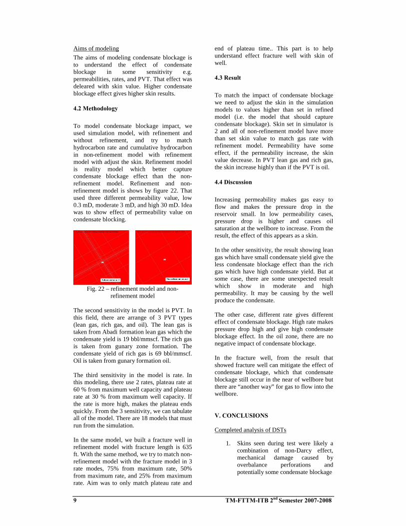
To model condensate blockage impact, we used simulation model, with refinement and without refinement, and try to match hydrocarbon rate and cumulative hydrocarbon in non-refinement model with refinement model with adjust the skin. Refinement model is reality model which better capture condensate blockage effect than the non-refinement model. Refinement and non-refinement model is shows by figure 22. Thatused three different permeability value, low 0.3 mD, moderate 3 mD, and high 30 mD. Idea was to show effect of permeability value oncondensate blocking.

Fig. 22 – refinement model and non-refinement model

The second sensitivity in the model is PVT. In this field, there are arrange of 3 PVT types(lean gas, rich gas, and oil). The lean gas is taken from Abadi formation lean gas which the condensate yield is 19 bbl/mmscf. The rich gas is taken from gunary zone formation. The condensate yield of rich gas is 69 bbl/mmscf.Oil is taken from gunary formation oil.

The third sensitivity in the model is rate. In this modeling, there use 2 rates, plateau rate at 60 % from maximum well capacity and plateau rate at 30 % from maximum well capacity. If the rate is more high, makes the plateau endsquickly. From the 3 sensitivity, we can tabulateall of the model. There are 18 models that must run from the simulation.

In the same model, we built a fracture well in refinement model with fracture length is 635 ft. With the same method, we try to match non-refinement model with the fracture model in 3 rate modes, 75% from maximum rate, 50% from maximum rate, and 25% from maximum rate. Aim was to only match plateau rate and

end of plateau time.. This part is to helpunderstand effect fracture well with skin of well.

4.3 Result

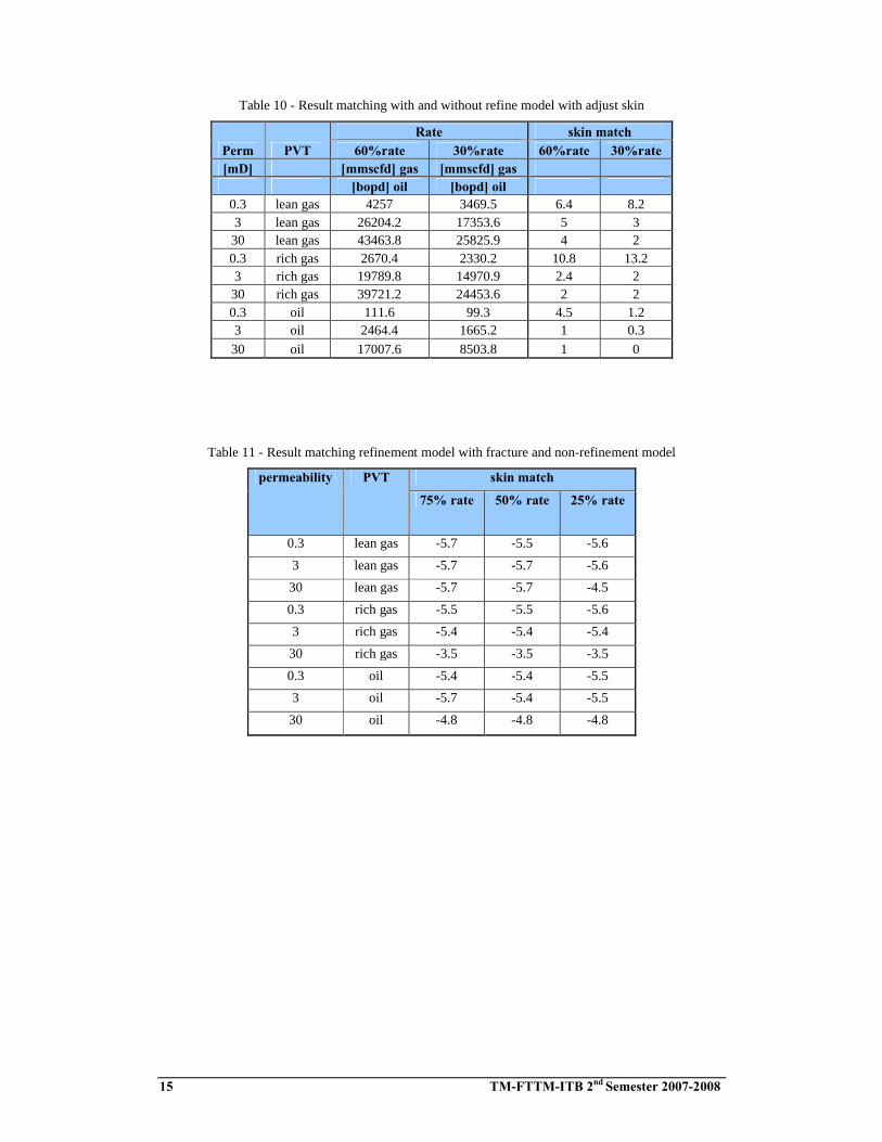
To match the impact of condensate blockage we need to adjust the skin in the simulation models to values higher than set in refined model (i.e. the model that should capture condensate blockage). Skin set in simulator is 2 and all of non-refinement model have more than set skin value to match gas rate with refinement model. Permeability have some effect, if the permeability increase, the skin value decrease. In PVT lean gas and rich gas, the skin increase highly than if the PVT is oil.

4.4 Discussion

Increasing permeability makes gas easy to flow and makes the pressure drop in the reservoir small. In low permeability cases, pressure drop is higher and causes oil saturation at the wellbore to increase. From the result, the effect of this appears as a skin.

In the other sensitivity, the result showing lean gas which have small condensate yield give the less condensate blockage effect than the rich gas which have high condensate yield. But at some case, there are some unexpected result which show in moderate and high permeability. It may be causing by the well produce the condensate.

The other case, different rate gives different effect of condensate blockage. High rate makespressure drop high and give high condensate blockage effect. In the oil zone, there are no negative impact of condensate blockage.

In the fracture well, from the result that showed fracture well can mitigate the effect of condensate blockage, which that condensate blockage still occur in the near of wellbore but there are “another way” for gas to flow into the wellbore.

V. CONCLUSIONS

Completed analysis of DSTs

1. Skins seen during test were likely a combination of non-Darcy effect, mechanical damage caused by overbalance perforations and potentially some condensate blockage


2. Boundaries observed in several wells at distance from 30 ft to 556 ft

3. Analysis remains subject to some uncertainty due to uncertainties in height of contributing zones

Constructed simulation sector model to compare DST results against simulation results (kh, skin, boundary)

1. simulation model may be morediscontinuous than actual results

2. permeability match is reasonably good

3. potential impact of condensate blockage observed in models

Constructed simulation sector model to understand condensate blockage and effect of hydraulic fractures at different rate, permeability, and PVTs

1. effect of condensate blockage increase if permeability decrease, liquid richness in gas increase and gas rates increase.

2. hydraulic fractures can help mitigate effects of condensate blockage

VI. RECOMMENDATIONS

1. Avoid overbalance perforation on DSTs to avoid risk of high skins

2. multi-rate flow are best practice to understand impact of non-Darcy skin

3. Run PLTs during testing to help determine flow contributions

4. Consider use of hydraulic fracture to mitigate effect of condensate blockage

5. In future modeling, tune the model against actual DST results (e.g. skin and boundaries)

NOMENCLATUREA = Area, sq ftD = Non-darcy skin, 1/mmscfddP = differential pressure, psih = net thickness of formation, ftk = Absolute permeability, mDkr = relative permeabilityL = length, ft = viscosity, cpm(P) = pseudo pressure function, psi2/cpP = pressure, psiq = gas rate, Mscf/dayS’ = total skinS = mechanically skin caused by

damage or stimulationz = gas deviation factor

REFERENCES

1. Dake, L.P : The Practice of Reservoir Engineering, Elsevier, Amsterdam

2. Craft, B.C. and Hawkins, M.F. : Applied Petroleum Reservoir Engineering, Prentice Hall, Inc., N.J., 1959.

3. Abdassah, Doddy : Teknik Gas Bumi, ITB, Bandung, 1998.

4. Abdassah, Doddy : Diktat Kuliah Analisis Transient Tekanan, ITB, Bandung, 1997.

5. Smith, C. R., Tracy, G. W., Farrar, R. L.: “Applied Reservoir Engineering”, Volume 2, OGCI Publications, Tulsa, Oklahoma, 1992.


Table 1 - Depth perforation and depth gauge

well test Zone depth test(ft KB) gauge depth (ft KB)Top Bottom

Well-2 DST#1 Abadi zone 26971 6979

6905.86986 6996

Well-3

DST#1 Gunary zone 4

8515 8520

8386.78594 86008656 86648814 8824

DST#1A Gunary zone 4

8515 8520

8386.7

8594 86008656 86648814 88248772 87868874 8888

DST-2 Gunary zone 1-2

7724 7734

7577.4

7753 77697800 78207915 79207930 79347950 7970

DST-2A Gunary zone 17724 7734

7578.67753 7769

DST-3 Abadi zone 1-4

6830 6840

6677.95

7028 70337057 70627107 71137120 71307159 71647210 72167452 74607564 7588

Well-5

DST-1 Gunary zone 2-3

7915 7935

7804.467960 79808026 8046

DST-2 Gunary zone 1 7525 7565 7440.66

DST-3 Abadi zone 3 7015 7055 6965.57

Table 2 - Porosity and ntg data (calculated from logging)

Well Test Zone ntg Φ net payWell-2 DST-1 Abadi zone 2 1.00 0.21 18.00

Well-3

DST-1 Gunary zone 4 0.87 0.15 25.26DST-1A Gunary zone 4 0.88 0.14 50.35DST-2 Gunary zone 1-2 0.98 0.18 73.56

DST-2A Gunary zone 1 0.96 0.19 25.04DST-3 Abadi zone 1-4 0.99 0.20 78.53

Well-5

DST-1 Gunary zone 2-3 0.62 0.13 37.07DST-2 Gunary zone 1 0.91 0.12 36.54

DST-3 Abadi zone 3 0.64 0.20 25.68


Table 3 - PVT Summary

Well DST Zone SG gas Oil CGR WGR Impurities [%] waterAPI chloride

[stb/mmscf] [stb/mmscf] H2S CO2 N2 [ppm]Well-2 DST-1 Abadi zone 2 0.765 51.4 30 Trace 0 0 0 trace

Well-3

DST-1 Gunary zone 4 0.706 51.6 18 10.25 0 1.71 0.49 9000DST-1A Gunary zone 4 0.706 51.6 18.6 9.67 0 1.71 0.49 19000DST-2 Gunary zone 1-2 0.864 51 143.7 1.9 0 4.59 0.26 18000

DST-2A Gunary zone 1 0.864 57.2 90 3.51 0 4.59 0.26 25000DST-3 Abadi zone 1-4 0.795 59.3 25.3 13.79 0 2.45 0.51 38000

Well-5

DST-1 Gunary zone 2-3 0.815 58.1 60.66 7.3 0 1.52 0.51 27000

DST-2 Gunary zone 1 0.81 57.3 46.51 5.16 0 1.89 0.5 43000

DST-3 Abadi zone 3 0.79 55.7 44.16 2.91 0 2.33 0.42 35000

Table 4 - DST Available data

Well Test # Zone Intervals Gas rate Cond rateft KB mmcf/d bcpd

Well-2 DST-1 Abadi zone 2 6,956 - 6,996 9.9 297

Well-3

DST-1 Gunary zone 4 8,515 - 8,824 11.8 211DST-1A Gunary zone 4 8,515 - 8,888 12 183DST-2 Gunary zone 1-2 7,724 - 7,970 12.4 1751

DST-2A Gunary zone 1 7,724 - 7,769 11.1 1000DST-3 Abadi zone 1-4 6,830 - 7,588 12.9 327

Well-5

DST-1 Gunary zone 2-3 7,915 - 8,046 6 359

DST-2 Gunary zone 1 7,525-7,565 7.1 338

DST-3 Abadi zone 3 7,015-7,055 17.4 783


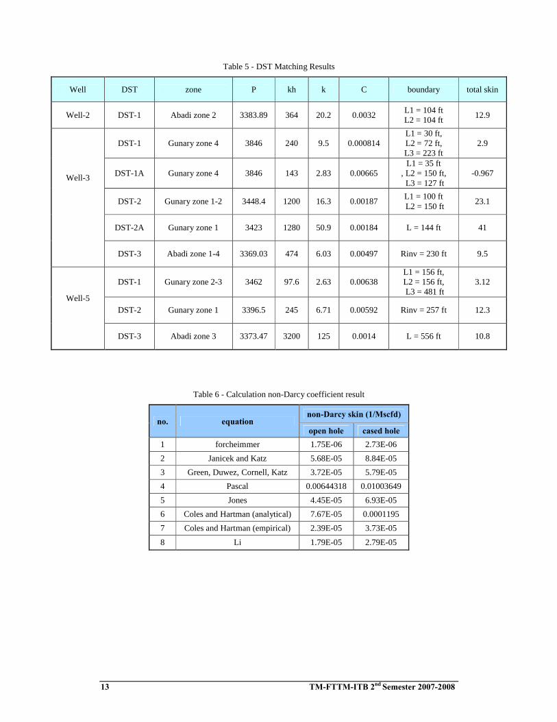
Table 5 - DST Matching Results

Well DST zone P kh k C boundary total skin

Well-2 DST-1 Abadi zone 2 3383.89 364 20.2 0.0032L1 = 104 ft L2 = 104 ft

12.9

Well-3

DST-1 Gunary zone 4 3846 240 9.5 0.000814L1 = 30 ft, L2 = 72 ft, L3 = 223 ft

2.9

DST-1A Gunary zone 4 3846 143 2.83 0.00665L1 = 35 ft

, L2 = 150 ft,L3 = 127 ft

-0.967

DST-2 Gunary zone 1-2 3448.4 1200 16.3 0.00187L1 = 100 ftL2 = 150 ft

23.1

DST-2A Gunary zone 1 3423 1280 50.9 0.00184 L = 144 ft 41

DST-3 Abadi zone 1-4 3369.03 474 6.03 0.00497 Rinv = 230 ft 9.5

Well-5

DST-1 Gunary zone 2-3 3462 97.6 2.63 0.00638L1 = 156 ft, L2 = 156 ft,L3 = 481 ft

3.12

DST-2 Gunary zone 1 3396.5 245 6.71 0.00592 Rinv = 257 ft 12.3

DST-3 Abadi zone 3 3373.47 3200 125 0.0014 L = 556 ft 10.8

Table 6 - Calculation non-Darcy coefficient result

no. equation non-Darcy skin (1/Mscfd)

open hole cased hole

1 forcheimmer 1.75E-06 2.73E-06

2 Janicek and Katz 5.68E-05 8.84E-05

3 Green, Duwez, Cornell, Katz 3.72E-05 5.79E-05

4 Pascal 0.00644318 0.01003649

5 Jones 4.45E-05 6.93E-05

6 Coles and Hartman (analytical) 7.67E-05 0.0001195

7 Coles and Hartman (empirical) 2.39E-05 3.73E-05

8 Li 1.79E-05 2.79E-05


Table 7 - Perforation Summary

Well DST fluid in hole Density spf perf type of gunswhen perforating fluid phasing

(ppg)Well-3 DST#1 Brine 10.1 12 135/45 atlas 4,5" high shoot density casing guns

DST#2 Brine 10.1 12 135/45 atlas 4,5" high shoot density casing gunsDST#2A Brine 10.1 12 135/45 atlas 4,5" high shoot density casing gunsDST#3 CaCl2 brine 11 12 135/45 atlas 4,5" high shoot density casing guns

Well-5 DST#1 CaCl brine 10.2 12 135/45 schlumberger 4,5" high shoot density casing gunsDST#2 CaCl brine 10.2 12 135/45 schlumberger 4,5" high shoot density casing gunsDST#3 CaCl brine 10.2 12 135/45 schlumberger 4,5" high shoot density casing guns

Well-2 DST#1 Seawater-gel 11.15 4 90 4" guns

Table 8 - Pressure when perforation summary

Well DST P wellbore (psia) P formation (psia) dP (psia) Skinwell-2 1 4001 3394 607 12.9

well-3

1 4429 3942 487 2.91A 4429 3942 487 -1.12 4014 3482 532 23.1

2A 4014 3482 532 413 3860 3381 479 9.5

well-5

1 4155 3489 666 3.12

2 3948 3417 531 12.3

3 3677 3374 303 10.8

Table 9 - Comparison between actual and simulation DSTs model

DST kh skin boundary

actual simulation actual simulation actual simulation

Well-3 DST3 474 394 9.5 4.8 no boundary L = 100 ft

Well-5 DST2 245 357 12.3 24.7 no boundary L = 70 ft, L = 400 ft, L 200 ft

Well-5 DST3 3200 3970 10.8 6 L = 556 ft L =130 ft , L = 130 ft


Table 10 - Result matching with and without refine model with adjust skin

Perm PVTRate skin match

60%rate 30%rate 60%rate 30%rate[mD] [mmscfd] gas [mmscfd] gas

[bopd] oil [bopd] oil0.3 lean gas 4257 3469.5 6.4 8.23 lean gas 26204.2 17353.6 5 330 lean gas 43463.8 25825.9 4 20.3 rich gas 2670.4 2330.2 10.8 13.23 rich gas 19789.8 14970.9 2.4 230 rich gas 39721.2 24453.6 2 20.3 oil 111.6 99.3 4.5 1.23 oil 2464.4 1665.2 1 0.3

30 oil 17007.6 8503.8 1 0

Table 11 - Result matching refinement model with fracture and non-refinement model

permeability PVT skin match

75% rate 50% rate 25% rate

0.3 lean gas -5.7 -5.5 -5.6

3 lean gas -5.7 -5.7 -5.6

30 lean gas -5.7 -5.7 -4.5

0.3 rich gas -5.5 -5.5 -5.6

3 rich gas -5.4 -5.4 -5.4

30 rich gas -3.5 -3.5 -3.5

0.3 oil -5.4 -5.4 -5.5

3 oil -5.7 -5.4 -5.5

30 oil -4.8 -4.8 -4.8

study of wellbore effect on drill stem test · pdf filewilly gunary abadi, 12204003, 2nd...

Documents