Study of the Gamma-Ray Universe from the GeV to TeV Range

Michelle D. Myers1

University of California, Berkeley

August 7, 2015

Nevis REU Summer 2015

Columbia, New York

ABSTRACT

Over one third of the entries in the third Fermi catalog (3FGL) are unidentified

and have no established multi-wavelength counterparts. To help identify these unas-

sociated sources, Fermi and VERITAS can be used to characterize sources in a wide

high-energy regime (20 MeV < E < 50 TeV). I present a maximum likelihood analysis

of two sources (3FGL J1250.2-0233 and 3FGL J2209.8-0450) in the hopes of estab-

lishing these to be viable sources for study by VERITAS. The analyses ultimately

result in finding possible counterparts in other catalogs. Additionally, I continue an

analysis of the BL Lac source B2 1215+30. This source shows correlated variability

in the Fermi and VERITAS energy ranges. In studying the variability of the source,

a limit on the Doppler factor of its relativistic jet can be derived, thus allowing for a

better understanding of the physics of active galaxies.

Contents

1 Introduction 2

2 The High-Energy Universe 4

2.1 Emission Mechanisms . . . . . . . . . . . . . . . . . . . . . . . . . . . . . . . . . . 4

2.2 Sources . . . . . . . . . . . . . . . . . . . . . . . . . . . . . . . . . . . . . . . . . . 6

2.3 Open Questions . . . . . . . . . . . . . . . . . . . . . . . . . . . . . . . . . . . . . 6

3 Observations 7

3.1 VERITAS . . . . . . . . . . . . . . . . . . . . . . . . . . . . . . . . . . . . . . . . 8

3.2 Fermi . . . . . . . . . . . . . . . . . . . . . . . . . . . . . . . . . . . . . . . . . . 8

1mmyers5@berkeley.edu

– 2 –

4 Fermi Analysis 9

4.1 Likelihood . . . . . . . . . . . . . . . . . . . . . . . . . . . . . . . . . . . . . . . . 10

5 Results 11

5.1 3FGL J1250.2-0233 . . . . . . . . . . . . . . . . . . . . . . . . . . . . . . . . . . . 13

5.2 3FGL J2209.8-0450 . . . . . . . . . . . . . . . . . . . . . . . . . . . . . . . . . . . 14

5.3 B2 1215+30 . . . . . . . . . . . . . . . . . . . . . . . . . . . . . . . . . . . . . . . 16

6 Summary and Conclusions 18

7 Acknowledgements 19

1. Introduction

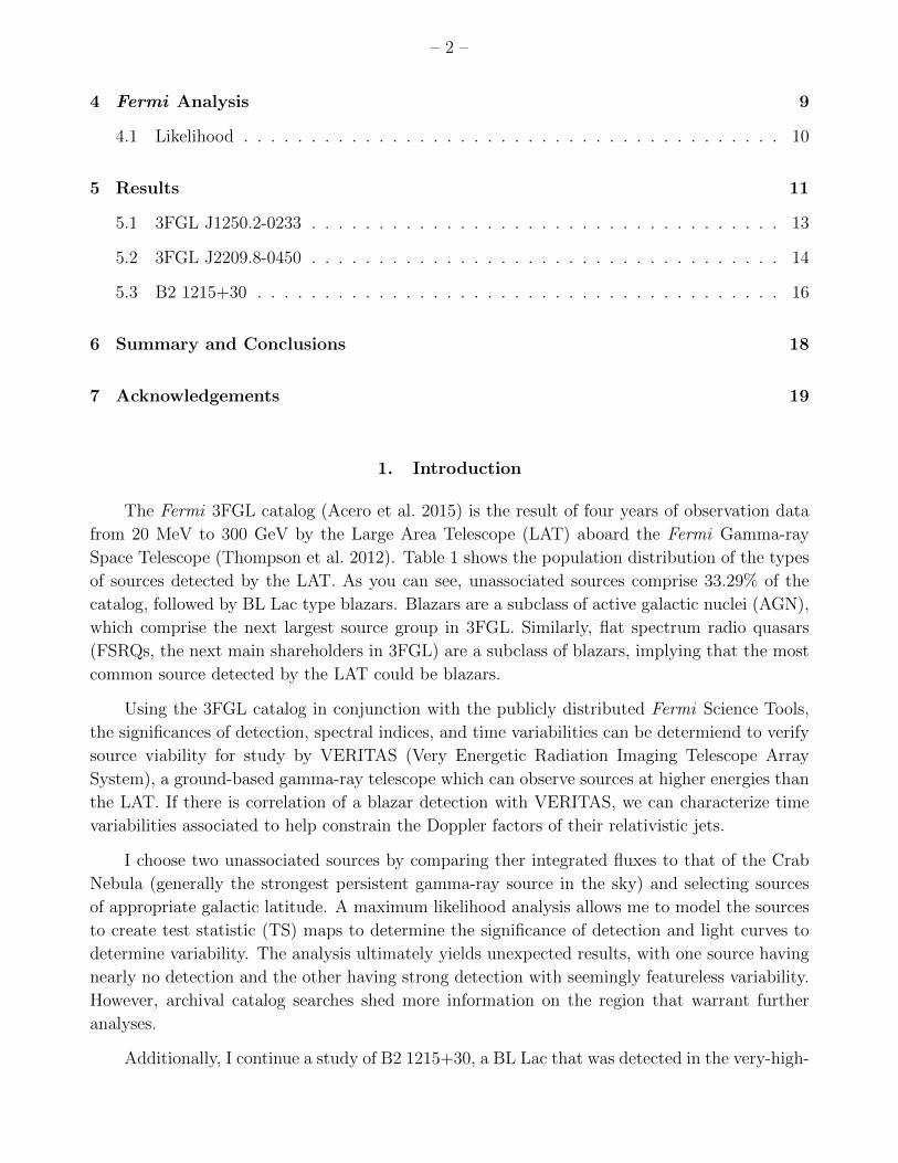
The Fermi 3FGL catalog (Acero et al. 2015) is the result of four years of observation data

from 20 MeV to 300 GeV by the Large Area Telescope (LAT) aboard the Fermi Gamma-ray

Space Telescope (Thompson et al. 2012). Table 1 shows the population distribution of the types

of sources detected by the LAT. As you can see, unassociated sources comprise 33.29% of the

catalog, followed by BL Lac type blazars. Blazars are a subclass of active galactic nuclei (AGN),

which comprise the next largest source group in 3FGL. Similarly, flat spectrum radio quasars

(FSRQs, the next main shareholders in 3FGL) are a subclass of blazars, implying that the most

common source detected by the LAT could be blazars.

Using the 3FGL catalog in conjunction with the publicly distributed Fermi Science Tools,

the significances of detection, spectral indices, and time variabilities can be determiend to verify

source viability for study by VERITAS (Very Energetic Radiation Imaging Telescope Array

System), a ground-based gamma-ray telescope which can observe sources at higher energies than

the LAT. If there is correlation of a blazar detection with VERITAS, we can characterize time

variabilities associated to help constrain the Doppler factors of their relativistic jets.

I choose two unassociated sources by comparing ther integrated fluxes to that of the Crab

Nebula (generally the strongest persistent gamma-ray source in the sky) and selecting sources

of appropriate galactic latitude. A maximum likelihood analysis allows me to model the sources

to create test statistic (TS) maps to determine the significance of detection and light curves to

determine variability. The analysis ultimately yields unexpected results, with one source having

nearly no detection and the other having strong detection with seemingly featureless variability.

However, archival catalog searches shed more information on the region that warrant further

analyses.

Additionally, I continue a study of B2 1215+30, a BL Lac that was detected in the very-high-

– 3 –

energy regime (E > 100 GeV) by MAGIC in 2011 (Aleksic et al. 2012). VERITAS detected and

performed an analysis using observational data from 2008 to 2012 (Aliu et al. 2013) and detected

variability as long as months. Another analysis was performed on VERITAS observation data

in 2014 in conjunction with LAT data to correlate time variability in both regimes (Zefi et al.

2015), resulting in a limit on the Doppler factor of the relatvistic jet from B2 1215+30.

Source Type Number of Entries Percent of 3FGL

Non-Blazar Active Galaxy 3 0.10%

Active Galaxy of Uncertain Type 573 18.89%

Binary 1 0.03%

BL Lac Blazar 660 21.75%

Compact Steep Spectrum Quasar 1 0.03%

Flat Spectrum Radio-Loud Quasar 484 15.95%

Normal Galaxy 3 0.10%

Globular Cluster 15 0.49%

High-Mass Binary 3 0.10%

Narrow-Line Seyfert 1 5 0.16%

Nova 1 0.03%

Pulsara 143 4.71%

Pulsarb 24 0.79%

Pulsar Wind Nebula 12 0.40%

Radio Galaxy 15 0.49%

Starburst Galaxy 4 0.13%

Seyfert Galaxy 1 0.03%

Star-Forming Region 1 0.03%

Supernova Remnant 23 0.76%

Special Casec 49 1.62%

Soft Spectrum Radio Quasar 3 0.10%

Unassociated 1010 33.29%

Table 1: The population of sources in 3FGL is dominantly unassociated, followed by BL Lac blazars.aIdentified by pulsations ; bNo pulsations seen by LAT ; cPotential association with supernova remnant or pulsar

wind nebula.

This paper will present a brief view of the gamma-ray sky and the types of mechanisms

and sources that occupy it. Open questions that can be explored by the study of gamma-rays

are suggested. Section 3 provides a discussion on instruments relevant to the project follows

to illuminate the utility of ground-based and space-based telescopes in complementary energy

regimes. The methods and parameters used in the analysis are outlined in Section 4, while

Section 5 reveals the results gained from the analysis.

– 4 –

2. The High-Energy Universe

The gamma-energy regime starts in the MeV range and extends to the TeV range, making

it difficult for any single telescope to observe this entire energy range. We typically associate

extreme galactic structures (supernovae, pulsars, quasars, black holes, etc...) with gamma-ray

sources. These exotic environments are capable of conditions that are effectively beyond what

we can recreate on Earth (e.g. extreme Lorentz factors). However, detection of gamma-rays in

the sky is non-trivial due to the attenuation of gamma-rays in space. For example, secondary

processes along the beam path enable us to detect gamma-rays from very distant blazars (Essey

et al. 2011). This section is concerned with the emission processes associated with gamma-ray

sources and the questions we have yet answered regarding them. Sections 3.1 and 3.2 illuminate

the instrumental methods of gamma-ray detection.

2.1. Emission Mechanisms

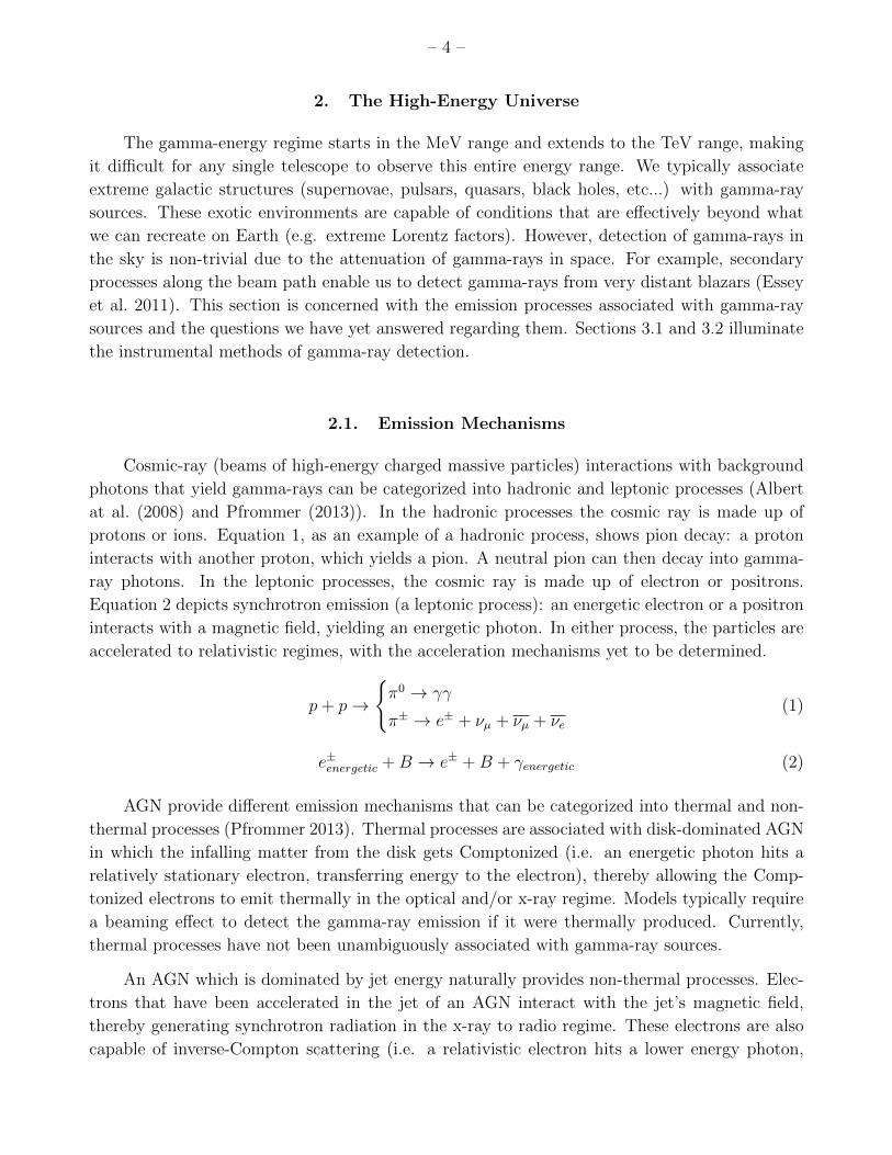
Cosmic-ray (beams of high-energy charged massive particles) interactions with background

photons that yield gamma-rays can be categorized into hadronic and leptonic processes (Albert

at al. (2008) and Pfrommer (2013)). In the hadronic processes the cosmic ray is made up of

protons or ions. Equation 1, as an example of a hadronic process, shows pion decay: a proton

interacts with another proton, which yields a pion. A neutral pion can then decay into gamma-

ray photons. In the leptonic processes, the cosmic ray is made up of electron or positrons.

Equation 2 depicts synchrotron emission (a leptonic process): an energetic electron or a positron

interacts with a magnetic field, yielding an energetic photon. In either process, the particles are

accelerated to relativistic regimes, with the acceleration mechanisms yet to be determined.

p+ p→

{π0 → γγ

π± → e± + νµ + νµ + νe(1)

e±energetic +B → e± +B + γenergetic (2)

AGN provide different emission mechanisms that can be categorized into thermal and non-

thermal processes (Pfrommer 2013). Thermal processes are associated with disk-dominated AGN

in which the infalling matter from the disk gets Comptonized (i.e. an energetic photon hits a

relatively stationary electron, transferring energy to the electron), thereby allowing the Comp-

tonized electrons to emit thermally in the optical and/or x-ray regime. Models typically require

a beaming effect to detect the gamma-ray emission if it were thermally produced. Currently,

thermal processes have not been unambiguously associated with gamma-ray sources.

An AGN which is dominated by jet energy naturally provides non-thermal processes. Elec-

trons that have been accelerated in the jet of an AGN interact with the jet’s magnetic field,

thereby generating synchrotron radiation in the x-ray to radio regime. These electrons are also

capable of inverse-Compton scattering (i.e. a relativistic electron hits a lower energy photon,

– 5 –

transferring energy to the photon) photons that are either generated by the synchrotron radia-

tion (synchrotron self-Compton) or by some external photon source such as ultraviolet radiation

from the disk. The two emission processes resultant from these accelerated electrons result in

a spectral energy distribution (SED) of the AGN with two distinct peaks (see Figure 1). The

synchrotron radiation photons emitted by the electrons are also capable of interacting with a

proton to create a pion, thus lending some ambiguity into whether or not the second emission

peak is a consequence of hadronic (protons) or leptonic (electrons) processes.

Fig. 1.— The figure on the left is an artistic render of an AGN. Jet orientation relative to our line of sight help

classify AGN into radio galaxies, quasars, and blazars. The figure on the right depicts blazar SEDs studied by

Donato et al. (2001) in attempt to unify blazar emission behaviors into one parameter: bolometric luminosity.

The lower-energy peak corresponds to synchrotron radiation emitted by electrons accelerated by the AGN jet.

The higher-energy peak corresponds to inverse-Compton radiation from electrons interacting with photons or

through pion decay. Blazars can be classified depending on their behavior in the optical regime. Also note how

higher-energy emission peaks correspond to lower luminosities.

The jet which provides for the non-thermal jet allows for the gamma-rays to exhibit a larger

luminosity than we would otherwise observe through aberration, time dilation, and red- (or blue-

) shifts. A measure of these effects, which essentially speaks to the strength of the jet, is the

Doppler factor (Dondi et al. 1995), which is given by

δ = [Γ(1− βcosθ)]−1 (3)

where Γ represents the Lorentz factor (Γ = 1√1−β2

) and β = vc. For an example of how the

Doppler factor can be constrained, see Section 5.3.

– 6 –

2.2. Sources

As mentioned above, AGN with jets are able to provide non-thermal processes for the

detection of gamma-rays. At the center of gamma-ray source galaxies are compact objects which

form twin ultra-relativistic jets from the accretion of matter in the disk (Urry et al. 1995). We

further subdivide radio-loud AGN into radio galaxies, quasars, and blazars depending on the jet

orientation relative to our line of sight (see Figure 1). Radio galaxies have jets perpendicular

to our line of sight, quasars have jets angled to our line of sight, and blazars have jets aligned

nearly directly to our line of sight.

Blazars, the most commonly detected gamma-ray sources in the sky, can be further classified

according to their multi-wavelength behavior. In Figure 1, we can distinguish between two main

subclasses depending on the behavior in the optical region. FSRQs have broad optical emission

lines with synchrotron emission peaking in the infrared regime, subsequently limiting the inverse-

Compton emission to the soft gamma-ray regime. Their lower energy emission also typically

allows for the greater observed luminosities due to energy-dependent gamma-ray attenuation in

space (higher energy gamma-rays are more attenuated). The second subclass of blazars is BL Lac

objects, which can have synchrotron peaks in the far-infrared, optical, or ultraviolet bands (and

sometimes even in the x-ray and gamma-ray bands), subsequently allowing for higher energy

inverse compton emission peaks.

Gamma-ray production is not limited to radio-loud AGN. For example, starburst galaxies

(galaxies with significant amounts of star-forming regions and, in effect, supernovae) with gamma-

ray components were first detected by VERITAS (Galante 2011). They have high densities

of cosmic rays that interact with interstellar gas and radiation, thus providing a non-thermal

mechanism by which gamma-rays are emitted (Acciari et al. 2009). Table 1 can help illuminate

the different types of sources that are capable of gamma-ray emissions. At the heart of all of the

processes lie non-thermal mechanisms to combat the attenuation of gamma-rays in space.

2.3. Open Questions

Aside from constraining the various emission mechanisms of gamma-ray sources (leptonic

vs. hadronic processes, for example), there are many open questions to be answered regarding

high-energy astrophysics that can be understood by studying gamma-ray sources. Constraining

beam properties of blazars, for example, allows us to study cosmological structures. Extra-

galactic background light (EBL) arise from photons that have been emitted by galaxies and other

galactic structures over the course of history. It is akin to the cosmic microwave background

(CMB) radiation with a higher registered energy. Unlike the CMB, the EBL cannot yet be

directly detected due to the abundance of foreground and galactic emission. To circumvent this

obstacle, absorption features of gamma-ray spectra can help reveal EBL properties. Attenuation

of gamma-ray flux in space is, in part, associated with gamma-ray photons pair producing with

EBL photons in the optical to ultraviolet bands, and we expect to see absorption features in

– 7 –

these bands of blazar SEDs. If the SED of an object is known, EBL density along the line of

sight can subsequently be inferred (Schroedter 2005).

Further, ultra-relativistic electron-positron pairs resulting from TeV photons annihilating

on the EBL are thought to lose energy by inverse-Compton scattering off of the CMB, cascading

the TeV emission down to GeV energies (Pfrommer 2013). GeV emission, however, is not ob-

served. Two mechanisms have been posited to be responsible for the absence of GeV emission:

intergalactic magnetic fields (IMFs) and blazar heating ((Arlen 2013) and (Chang et. al 2012),

respectively). IMFs are thought to deflect the electron-positron pairs out of the line of sight,

allowing limits to be placed on IMF strengths. Blazar heating, a more effective mechanism for

”hiding” the GeV emission, involves the propagation of the ultra-relativistic electron-positron

pairs through the intergalactic medium. They are subsequently subjected to plasma instabilities

which ultimately result in heat being transferred to the intergalactic medium.

Blazar time variability also exhibit complex multi-wavelength behavior (Pfrommer 2013)

that cannot be modeled simply. Variability timescales range from the order of minutes (Aharo-

nian et al. 2008) to years (Ruan et al. 2012), with small time-scales correlating to super compact

emission regions and large Lorentz factors (Begelman et al. 2008).

Despite the ambiguity of the emission mechanisms that result in the differing timescales,

quantum gravity theories can also be tested using the variabilities observed. Lorentz invariance

violations (LIVs), for example, should be observed at Planck-scale energies. Looking at the

propagation of gamma-rays at the Crab pulsar at different energies allows constraints to be

placed on LIVs (Zitzer 2013).

The energy regime of gamma-rays also correspond to the energy regime of electroweak force

interactions, which coincides with dark matter particle masses of weakly interacting massive

particles (WIMPs) (Steigman et al. 2012). The relic density of WIMPs is the amount of WIMPs

we currently observe given that they were created thermally. As the universe cooled, WIMP

creation would cease, allowing the population density to decrease as they annihilated with other

WIMPs. A cross-section can be calculated to account for the current WIMP density (i.e. the

probability for WIMP annihilation is very low), which subsequently constrains WIMP masses.

Acciari et al. (2010) outline a method by which observations of gamma-rays from dark-matter

dominated galaxies can constrain cross sections and relative velocities of WIMPs.

3. Observations

VERITAS can observe objects in with energies 50 GeV < E < 50 TeV, while Fermi can

observe at 20 MeV < E < 300 GeV. Together, they form a complementary and broad energy

range for study of gamma-ray sources. The different energy regimes are realized by two different

detection methods: indirect and direct.

– 8 –

Fig. 2.— The figures above depict the Fermi Gamma-Ray Space Telescope on the left and the

four Cherenkov telescopes associated with VERITAS on the right.

3.1. VERITAS

Gamma-rays cannot penetrate the Earth’s atmosphere, but we can detect Cherenkov radi-

ation from incident gamma-rays in the atmosphere (Galbraith et al. 1953). Incident gamma-

rays (and cosmic-rays) trigger particle cascades of relativistic charged particles which create

Cherenkov radiation in the direction of propagation. The shower creates a light pool on the

ground that peaks roughly in the optical range (∼400 nm wavelength which corresponds to blue

light) for high-energy incident events. VERITAS subsequently uses mirrors to reflect the light

onto a focal plane camera (Holder et al. 2006) to image the showers (see Figure 2).

Located at the Fred Lawrence Whipple Observatory in southern Arizona, VERITAS is

comprised of four 12 meter optical reflectors, achieving maximum sensitivity for incident rays

with energies 85 GeV < E < 10 TeV. Both cosmic-rays and gamma-rays can induce particle

showers in Earth’s atmosphere. Cosmic-ray events can be distinguished from gamma-ray events

depending on their image orientation and morphology; cosmic-rays are generally wider and less

regular because the showers generally have several components. When the particle showers are

observed by Cherenkov telescopes, they appear as elongated ellipses from which the original

direction of propagation can be derived (Hillas 1985). By analyzing the Cherenkov yield from

the particle shower of a gamma-ray event, VERITAS is also able to discern the original energy

of the incident gamma-ray.

3.2. Fermi

The Fermi LAT aboard the Fermi Gamma-Ray Space Telescope, which was launched in

June 2008, has a detection range of 20 MeV < E < 300 GeV. Direct detection of gamma-rays

must occur in outer space, which limits the collection area and, therefore, the flux that can be

received by space telescopes. Using adapted accelerator experiment techniques (Thompson et al.

2012), the LAT uses a layer of tungsten to convert incoming gamma-rays into electron-positron

pairs. The pairs then interact with silicon-strip charged-particle trackers to create images of the

pair trajectory, after which a calorimeter measures the energies of the particles. It has an angular

– 9 –

resolution finer than 1◦ for a single gamma-ray, has a large field of view (20◦), and can observe

the entire sky every three hours.

Cosmic-rays also pose a problem to the LAT; there is 105 more cosmic-ray flux than gamma-

ray flux. An Anticoincidence Detecter rejects 99.97% of cosmic-ray signals incident on the LAT

by distinguishing between charged particle events and neutral (gamma-ray) events. Further, the

LAT also filters against gamma-rays that originate in Earth’s atmosphere. Similar to VERI-

TAS, the Fermi LAT determines the incident energies and directions of propagation of incoming

gamma-rays.

4. Fermi Analysis

An unbinned maximum likelihood analysis was performed on specifically chosen sources

from the 3FGL catalog using survey data by the Fermi LAT. The analysis used the Fermi

Science Tools software package, version v10r0p51, in the Python environment. The procedure

is initiated by running gtselect to make cuts on energy and time of the data sets downloaded

from the Fermi database. These cuts take into account the source region (the distance out to

which sources from the 3FGL catalog were included in the model) and the region of interest

(the distance out to which photon counts from sources form the 3FGL catalog were allowed to

have free parameters). Due to the energy-depencies of the point spread function of the LAT, for

analyses with energies E ∼ 1 GeV, it is recommended to use a 15◦ source region with a 5◦ region

of interest. For lower energies (E ∼ 100 MeV), the source region is recommended to be 20◦ with

a 10◦ region of interest2.

Using gtmktime subsequently filters the data set further to create good time intervals (GTIs),

i.e. time periods wherein the data are valid, using spacecraft data from the database. gtbin

then allows for the creation of a counts map, one of the first indicators of a viable data set. The

counts maps is a two-dimensional spatial map that shows photon counts that reflect the various

filteres already placed on the data set. Lack of counts in the area where a detection is expected

may indicate the need for less stringent cuts on time and energy.

The most time-consuming part of the analysis comes from creating exposure maps (gtexpmap)

and livetime cubes (gtltcube) necessary for computing the predicted numver of photons in the

region of interest. In conjunction with those processes make3FGLxml.py3 was used to generate

an XML file to create a model file based on 3FGL catalog sources, using gll_iem_v06 and

iso_P8R2_SOURCE_V6_v064 as the galactic diffuse and isotropic model files, respectively.

1http://fermi.gsfc.nasa.gov/ssc/data/analysis/software/

2http://fermi.gsfc.nasa.gov/ssc/data/analysis/documentation/Cicerone/Cicerone Likelihood/Choose Data.html

3http://fermi.gsfc.nasa.gov/ssc/data/analysis/user/ by T.Johnson

4http://fermi.gsfc.nasa.gov/ssc/data/access/lat/BackgroundModels.html

– 10 –

After the source model is generated, gtdiffrsp can be run to save time durring the maxi-

mum likelihood analysis. This function convolves the source model with the instrument response

function, and can be particularly extensive for diffuse sources. This, as well as the exposure

maps and the livetime cubes, need only to be executed once as long as cuts on the data set

are not changed. Maximmum likelihood analyses can be performed on the data set with small

changes in the source model file. For the analyses reported, gtlike is invoked twice to per-

form a maximum likelihood analysis: once with a DRMNFB optimizer, the results of which are

used perform another maximum likelihood analysis with a NewMinuit optimizer. This treatment

combines the ability for the DRMFB optimizer to converge more quickly at the cost of param-

eter depence information with the special attention that the NewMinuit optimizer pays to the

parameter space.

Results of the analysis include light curves, test-statistic (TS) maps, and SEDs. Light curves

depict the time variability of a source by presenting flux as a function of time. TS maps are a

test of the probability of the model being statistically significant. SEDs represent the spectral

behavior of sources by presenting luminosity as a function of energy. Note that the likelihood

analysis performed here does not localize the source (although there are methods by which source

localization could be achieved). Rather, the analysis presented is used to fit models to the data

and to determine detection significance.

4.1. Likelihood

Likelikhood (L) is a measure of how likely a model can recreate observational data. The

data are binned spatially such that the expected number of counts in the ith bin is mi, which is

calculated from the model. The probability pi of getting ni counts (taken from the data) in the

bin is

pi =mnii e−mi

ni!(4)

The likelihood is the product of pi over all i. We can simplify this a little bit further by realizing

that the product over all i of e−mi is equal to e−Σimi , with Σimi being the total number Nexp of

expected counts that the source model predicts. As a result, we get

L = e−NexpΠimnii

ni!(5)

This summarizes a binned likelihood analysis. To perform an unbinned analysis, we allow the

bin sizes to get infintesimally small such that ni = 0 or 1, allowing us to rewrite Equation 5 as

L = e−NexpΠimi (6)

Detection significance can be determined through the TS, which is defined as

TS = −2 ln(LnullL

) (7)

– 11 –

where Lnull is the likelihood corresponding to the null hypothesis (a model that is slightly modified

from the original model, e.g. comparing a model with an absent source versus a model with a

present source). A lower Lnull indicates that the null hypothesis is incorrect, which corresponds

to a larger TS. In maximizing the likelihood of the model, the detection significance is maximized.

Additionally,√TS corresponds to the σ level of detection.

5. Results

In the 3FGL catalog, there are 1059 unassociated sources. To narrow down the candidates

for VERITAS, I computed the integrated fluxes of the unassociated sources and compared them

to that of the Crab Nebula.

F =

∫ ∞Eth

N0[E

E0

]−γdE (8)

This assumes the form of a power law for the source, which is the common choice, where N0, E0,

and γ correspond to the flux density, pivot energy, and spectral index of the source, respectively.

Eth = 80 GeV for the purpose of choosing an energy threshold near the maximum sensitivity of

VERITAS. Table 2 quantifies the results of the sources that had an integrated flux > 2% than

that of the Crab Nebula integrated flux. Two of the sources are flagged as being in a very bright

region, while one is flagged as an extended source. Sources with a high galactic latitude (away

from the diffuse emission of the disk) were given higher priority to reduce the diffuse emission

components from other high-energy sources (see Figure 4). The two sources chosen are marked

clearly in Figure 3 (3FGL J1250.2-0233, 3FGL J2209.8-0450).

Source Name Integrated Flux (photonscm2s

) Percent of Crab

J1250.2-0233 1.67×10−10 9.6%

J1552.9-5610 4.68×10−11 2.7%

J1615.3-5146e 2.14×10−10 12.3%

J1640.4-4634c 7.52×10−11 4.3%

J1745.6-2859c 6.66×10−11 3.8%

J1829.2-1504 4.17×10−11 2.4%

J1834.6-0659 4.39×10−11 2.5%

J1838.9-0646 4.68×10−11 2.7%

J2053.9+2922 3.72×10−11 2.1%

J2209.8-0450 7.87×10−11 4.5%

Table 2: The results of the analysis comparing the integrated fluxes of unassociated sources with the Crab

Nebula flux are shown in the table above. Source names followed by ’e’ are flagged as extended sources while ’c’

signifies that the source is in a region with bright and/or possible incorrecrtly modeled diffuse emission.

In addition to the two unidentified sources, I looked at a blazar detected by VERITAS that

is also an identified Fermi source. B2 1215+30, a BL Lac, has been studied by the VERITAS

– 12 –

Fig. 3.— A sky map showing all of the unassociated sources in 3FGL in galactic coordinates. Sources found

with integrated fluxes > 2% compared to the Crab Nebula Flux are indicated in color. Blazar B2 1215+30 is

labelled as well. Note the population density of unassociated sources near the galactic center.

Fig. 4.— The figures above show the population distribution of 3FGL unassociated sources. Note the more

isotropic distribution in the longitudinal space in contrast to the narrower distribution near the galactic disk (at

latitude 0◦).

– 13 –

Collaboration both using a VERITAS Eventdisplay analysis and a Fermi Science Tools analysis

(Zefi et al. 2015). I continue that research by conducting a Fermi analysis and compare my

results to the past analyses.

5.1. 3FGL J1250.2-0233

3FGL J1250.2-0233 is located at (α, δ) = (12h50m16.320s,−02◦33′50.40′′) with 9.6% Crab

Nebula flux (see Table 2) and a given spectral index γ = 1.10 . The data used are from the same

dataset used to create the catalog (2008-2012). Due to the presence of 3FGL J1256.1-0547 (or

3C 279, an optically violent variable and among the brightest gamma-ray objects observed in

the sky) within the region of interest, I elected to constrain the energy range of my analysis to 5

GeV < E < 100 GeV with a source region of 10◦ and an ROI of 5◦. Reviewing the counts map

(see Figure 5) revealed significantly less activity from 3C 279 in the years 2008 to 2010, allowing

for further constraints on the data set to better detect 3FGL J1250.2-0233 against the diffuse

background emission.

A maximum likelihood analysis of the data gives a meager TS value of 4.16 (see Figure 5)

with a spectral index γ ' 0. Given that there is not an abundance of photon counts at the source

Fig. 5.— The figure in the left is a photon counts map with a source model, centered around 3FGL J1250.2-

0233. The colorbar denotes the number of photon counts. The figure on the right is a TS map given a 5◦ region

of interest and a 10◦ source region. The colorbar denotes the TS at a given location. Note the lack of photon

counts or significance in the center of both maps.

location, it is not surprising that the TS maps suggest that there is no source. Improvements

in modeling diffuse and isotropic emission since the catalog’s release may help account for the

null detection of the source. Additionally, the likelihood analysis may have failed in part due to

stringent cuts made on energy. Without enough photon counts to characterize the source, the

modeling process suffers from large uncertainties. Including more energy bands will be conducive

to characterizing 3FGL J1250.2-0233.

– 14 –

The TS map, however, suggests that there is a source located at (α, δ) =∼ (12h46m,+01◦).

This object is identified as a BL Lac object in the 5th edition of the Roma-BZCAT catalog

(Massaro et al. 2009) and is labeled in the counts map in Figure 5 as 5BZB J1246+0113 at

(α, δ) = (12h46m02.500s,+01◦13′18.80′′). Further analyses of 5BZB J1246+0113 will be initi-

tated to discover its properties in the Fermi range. The utility of the Fermi Science Tools to

uncover sources not included in the catalog, even as an unassociated source, is thus validated.

5.2. 3FGL J2209.8-0450

3FGL J2209.8-0450 is located at (α, δ) = (22h09m52.080s,−046◦51′00.00′′) with 4.5% Crab

Nebula flux (see Table 2) and a given spectral index γ = 1.27. Similar to the source in Section

5.1, the data came from 2008-2010. The energy range was extended to include 1 GeV < E <

300 GeV after seeing structure in the counts maps at these energies, allowinf for a source region

of 10◦ and an ROI of 5◦.

In the most recent analysis performed (see Figure 6 for a preliminary TS map), 3FGL

J2209.8-0450 was detected with a TS of 36.876 and a spectral index γ = 1.3± 0.3, suggesting a

good source detection.

Fig. 6.— The figure in the left is a photon counts map with a source model, centered around 3FGL J2209.8-0454.

The figure on the right is a preliminary TS map given a 5◦ region of interest and a 10◦ source region.

Given a statistically significant detection, the analysis was continued to generate light curves.

Ultimately, the light curve featured in Figure 7 results from data taken from 2008-2012 binned

into 4 energy bins and monthly time bins. Upper limits were calculated for time bins with TS

< 9. A longer time period may reveal variability over a long timescale as some blazars have

variability on the order of years (Ruan et al. 2012). The possibility of a flare occurring in March

2011 is also worth investigating.

Further, a catalog search for this source yielded results from a Swift-XRT survey that ob-

– 15 –

Fig. 7.— The light curve above shows 3FGL J2209.8-0450 flux over time. Data are binned into 4 energy bins

and monthly time bins. Upper limits are calculated for TS < 9.

served unassociated sources from the 3FGL catalog. These results are displayed in Figure 8.

Accoridngly, Swift detects both an x-ray (RXS J220942.1-045120) and a radio (NVSS J220941-

045111) source located within the error circle provided by 3FGL for this source. 3FGL J2209.8-

0450 could very well be the gamma-ray counterparts to these sources.

Fig. 8.— The figures above are from the Swift-XRT survey of Fermi unassociated sources, where the x-axis and

y-axis correspond to right ascension and declination repesctively. The plots are centered on 3FGL J2209.8-0450

with an error circle provided by 3FGL. The figure on the left reveals that there is an x-ray source within the error

circle, while the figure on the right shows that there is a correlated radio source in the error circle as well.

– 16 –

5.3. B2 1215+30

B2 1215+30 is located at (α, δ) = (12h17m51.60s,−30◦07′04.80′′) with 4.9% Crab Nebula

flux and a given spectral index γ = 1.97. Following an earlier analysis (Zefi et al. 2015), I

performed the analysis with an energy range 100 MeV < E < 100 GeV with time taken from

January to July in the year 2015. Consequently, the source region is 20◦ with an ROI of 10◦.

The SED of B2 1215+30 is shown in Figure 9 (Prokoph 2013).

Fig. 9.— Spectral energy distribution of B2 1215+30 during 2011 model assuming a redshift of z = 0.130 (solid

lines) and a redshift of z = 0.237 (dashed lines).The blue lines represent the model for the low x-ray state in

January and the red lines the model for the high x-ray state in April/May, respectively. The inset on the right

focuses on the inverse-Compton emission peak. See Prokoph (2013) for more information.

In the analysis, B2 1215+30 is detected with a TS of 4143.14 and a spectral index γ =

1.90±0.02. The TS map depicted in Figure 10 show preliminary results that do not reflect more

recent models used in the upcoming light curves. Updated TS maps will be forthcoming.

Figure 11 shows the light curves generated from past analyses and the current analysis.

The left image illustrates the similarities in the separate analyses performed using Fermi Science

Tools. The data are binned into 8 energy bins and 3-day bins for both analyses in. The image

on the right shows data from the 2015 analysis binned in 8 energy bins and in both 3-day and

1-day bins. Figure 11 indicates that a flare occurred during the months of June and July 2015.

Treatment of the flare data could place limits on the Doppler factor, an example of which follows.

A flare, detected both by Fermi and VERITAS, in February 2014 was analyzed in Zefi et

al. (2015) to derive a limit for the Doppler factor of the relativistic jet of B2 1215+30. The light

curve can be formalized as follows:

F (t) = Fc + F0 ×2t−t0

tvar(9)

where Fc, F0, and tvar represent the average source flux, flux of the flare at t0, and the variability

time scale, respectively. It should be noted that Equation 9 represents the rising side of the flare.

Performing an appropriate fit on the light curve allows for a value of tvar to be computed, which

– 17 –

Fig. 10.— The preliminary TS map of B2 1215+30 is represented above. Note the strong detection of the

source. More recent models remove much of the residual feedback.

Fig. 11.— The figures above depict light curves of B2 1215+30. The left figure overlays the analysis performed

by Zefi et al. (2015). The right figure illustrates the light curves binned in 3-day bins (the blue data points) and

1-day bins (the green data points).

– 18 –

is the time in which flux doubles. Zefi et al. (2015) re-formalize the Doppler factor as follows

(Dondi et al. 1995):

δ ≥ [σt × d2

L

5hc2(1 + z)2αF1keV

tvar(EγGeV

)α)]1

4+2α (10)

where dL represents the luminosity distance, α represents the x-ray spectral index, F1keV repre-

sents the flux received at 1keV, and Eγ represents that higher-energy photon. Treatment by Zefi

et al. (2015) reports a Doppler factor δ ≥ 5.7.

6. Summary and Conclusions

This paper was an exercise in providing an overview of the gamma-ray universe with empha-

sis on the most commonly detected gamma-ray sources–blazars. It covers the various emission

mechanisms to reveal the need for non-thermal mechanisms and how different source types meet

this demand, then poses a few questions faced by astrophysicists today.

A brief treatment of the different ways in which gamma-rays are detected is shown by

including two vastly different instruments–VERITAS and the Fermi LAT. Subsequently, the

methods used to analyze Fermi data rely on a maximum likelihood analysis. Three sources

(3FGL J1250.02-0233, 3FGL J2209.8-0450, and B2 1215+30) are chosen to receive this treatment.

Of the two unassociated 3FGL sources analyzed, only 3FGL J2209.8-0450 was confidently

detected. Further analysis of this source in an attempt to characterize its variability timescale

is recommended, with less stringent cuts on the energy band. However, the steepness of the

spectrum as indicated by its spectral index may still limit the received flux.

Though 3FGL J1250.2-0233 is not confidently detected, a nearby source has been detected

that is not included in the 3FGL catalog. This confirms the ability of the likelihood analysis to be

able to detect local, un-modeled sources. Study of this source should be continued to constrain

its properties in the Fermi range.

B2 1215+30 provides a promising source of study due to the significant detection by the

LAT. The light curves from the analysis indicate that the source was in a flaring state during

June/July of 2015. Further inspection should allow for another analysis to constrain the Doppler

factor of the relativistic jet of the source.

Ultimately, we have much more to learn about the gamma-ray and non-thermal universe,

from the emission mechanisms that enable detection of gamma-ray sources to to the consequences

of gamma-ray sources propagating through space.

– 19 –

7. Acknowledgements

I would like to thank Reshmi Mukherjee, Marcos Santander, and Brian Humensky for their

guidance in this project. I thank John Parsons, Mike Shaevitz, and the Nevis Labs staff and

faculty for establishing a respectable internship and undergraduate research opportunities. This

work was funded by the National Science Foundation.

REFERENCES

V.A. Acciari et al. (The VERITAS Collaboration), ApJ 720, 1174 (2010)

V.A. Acciari et al. (The VERITAS Collaboration), Nature 472, 770 (2009)

F. Acero et al. (The Fermi Collaboration), arXiv: 1501.02003 (2015)

F. Aharonian et al. (The HESS Collaboration), Phys. Rev. Lett. 101, 261104 (2008)

M. Akiyama, Y. Ueda, K. Ohta, T. Takahashi, T. Yamada, ApJS 148, 275 (2003)

J. Albert et al. (The MAGIC Collaboration), Science 320, 1752 (2008)

J. Aldrich, Statistical Science 12, 162

J. Aleksic et al. (the MAGIC Collaboration), A&A 544, A142 (2012)

E. Aliu et al. (The VERITAS Collaboration), ApJ 779, 92 (2013)

T. Arlen, PhD thesis, University of California Los Angeles Dept. of Physics (2013)

M.C. Begelman, A.C. Fabian, M.J. Rees, MNRAS 384, L19 (2008)

P. Chang, A.E. Broderick, C. Pfrommer, ApJ 752, 23 (2012)

D. Donato, G. Ghisellini, G. Tagliaferri, G. Fossati, A&A 375, 739 (2001)

L. Dondi, G. Ghisellini, Mon. Not. R. Astron. Soc. 273, 583 (1995)

W. Essey, O. Kalashev, A. Kusenko, J.F. Beacom, ApJ 731, 51 (2011)

N. Galante, Fermi Symposium Proceedings, arXiv:1111.0244 (2011)

W. Galbraith, J.V. Jelley, Nature 171, 349 (1953)

A. Hillas, The 19th International Cosmic Ray Conference Proceedings (1985)

J. Holder et al., Astroparticle Physics 25, 391 (2006)

E. Massaro, A. Maselli, C. Leto, P. Marchegiani, M. Perri, P. Giommi, S. Piranomonte, arXiv:

1502.07755 (2009)

– 20 –

J.R. Mattox et al., ApJ 461, 396 (1996)

C. Pfrommer, subm. (2013) arXiv:1308.6582

H. Prokoph, PhD thesis, MathematischNaturwissenschaftlichen Fakultat I der Humboldt-

Universitat zu Berlin (2013)

J.J. Ruan et al., ApJ 760, 51 (2012)

M. Schroedter, ApJ 628, 617 (2005)

G. Steigman, B. Dasgupta, J.F. Beacom, Phys. Rev. D86, 023506 (2012)

D.J. Thompson, S.W. Digel, J.L. Racusin, Phys. Today 65, 39 (2012)

C. Urry, P. Padovani, PASP 107, 803 (1995)

R.L. White et al., ApJS 126, 133 (2000)

F. Zefi et al., The 34th International Cosmic Ray Coference Proceedings (2015)

B. Zitzer, ICRC Proceedings, arXiv:1307.8382 (2013)

This preprint was prepared with the AAS LATEX macros v5.2.