Ind

ust

rial E

lectr

ical En

gin

eerin

g a

nd

A

uto

matio

n

CODEN:LUTEDX/(TEIE-5458)/1-62(2021)

Study of an Automated Testing Procedure with Dynamic Job Scheduling and Automatic Error Handling

Tom Andersson

Division of Industrial Electrical Engineering and Automation Faculty of Engineering, Lund University

Study of an automated testing procedure with dynamic job

scheduling and automatic error handling

Tom Anderssontomandersson94@gmail.com

April 14, 2021

Abstract

During the production of Axis’s cameras, the optics modules have to do a number of tests and calibrationsthat are performed in different test stations. The test and calibration sequence differs between differentmodels. This has so far been done manually by having operators move the units between test stations.However, Axis are planning to automate the procedure by having an industrial robot move test unitsbetween the different test stations. The scope of this thesis is to come up with a concept for the controlof the system, including the flow of information and the job scheduling, and implement a simulationprogram where production sequences can be evaluated. The thesis is divided into four parts, specifyingthe system requirements, concept generation, scheduling analysis, and implementation of simulations.

The requirements of the system were formulated by discussing the vision of the system with theproject team at Axis. The essential requirements can be summarized as follows. The throughput of thesystem and the utilization of the different test stations should be as high as possible. It should be possibleto connect and disconnect test stations during production, without interrupting the rest of the system.The system should be able to automatically handle unexpected states, such as test units being moved,having units already within the system upon start up, test stations which break during production etc.The system should handle potential deadlock situations to keep the production running. And finally,relevant data concerning tests, test stations and the flow of production should be stored for traceabilityreasons and visualized to achieve an overview of the production.

During the concept generation two concepts were generated. One concept was based on the initialvisions of the project team at Axis. The fundamental idea with this concept is that information whichis both generated within the system and is needed further down the test sequence of a specific testunit is stored on an ID-tag, for example an RFID-tag, attached to that test unit. This information isthereafter read when the unit arrives to the different subsystems within the system. The other conceptwas generated more freely based on the knowledge and experience of the student carrying out the thesis.In this concept, the generated information is instead stored in a database and thereafter accessed by thedifferent subsystems within the system. It was concluded that both concepts offer similar functionalitiesbut the complexity of the ID-tag concept was lower. However, the project team at Axis was moreexperienced in working with databases compared to ID-tags and it was assessed that the lower complexityof the ID-tag concept was not significant enough to overlook the experience of the team. Therefore, thedatabase concept was recommended for a future implementation.

To achieve an efficient system, the theories of job shop scheduling are analysed. A framework fordynamic scheduling was studied to get an overview of how job scheduling problems can be solved. Forinstance, the framework described three different categories of dynamic scheduling approaches: heuristicrules, classical optimization and approaches based on artificial intelligence. Within these categories, acouple of major techniques were analysed namely 12 standardized heuristic rules for different objectives,the classical optimization techniques dynamic programming and branch and bound, A*, as well as theartificial intelligence approaches beam search, genetic algorithms, and tabu search. One technique fromeach category was also analysed on a deeper level with focus on the system concerned by this theses.These techniques were a combined heuristic rule focusing on throughput, A*, and beam search, wherethe last technique, beam search, is a combination of heuristic rules and A*.

iii

The implementation of the simulation was based one the database concept. The user specifies theavailable test stations, occurrence of breakdowns, buffer size, an incoming rate of test units with a giventest cycle, test units already placed inside the system upon start up, etc. The simulation program willthen run these sequences using the derived combined heuristic rule as well as specified time durations fortests and the movement of the robot. Once the simulations have completed, the user is presented withrelevant data such as total time, throughput, utilization factors etc. Optimally the simulations shouldalso include A* and beam search but this was not included in the simulations within the scope of thethesis.

This thesis provides a foundation for a future implementation of the system. The derived systemconcept can be used as a base for a future system design and the simulation software can be used toevaluate several production capabilities such as, how many test stations of each type that should be usedat a certain production rate.

iv

Preface

Years of studies have come to an end and all the knowledge and experience that have been acquiredthroughout the years are now applied in this thesis. I would like to thank everyone at Axis for giving methis opportunity, for supporting me throughout the thesis, and most of all, for making me feel welcome tothe team at Axis. A special thanks to my supervisors Bjorn Hansson and Martin Nyman, my academicsupervisor Gunnar Lindstedt, and my examiner Ulf Jeppsson for all the valuable guidance you have givenme during this project. Thank you, it would not have been possible without you.

v

vi

Contents

Acronyms and abbreviations ix

1 Introduction 1

2 System specifications 32.1 Fundamental functionality . . . . . . . . . . . . . . . . . . . . . . . . . . . . . . . . . . . . 32.2 Efficiency . . . . . . . . . . . . . . . . . . . . . . . . . . . . . . . . . . . . . . . . . . . . . 32.3 Flexibility . . . . . . . . . . . . . . . . . . . . . . . . . . . . . . . . . . . . . . . . . . . . . 42.4 Error handling . . . . . . . . . . . . . . . . . . . . . . . . . . . . . . . . . . . . . . . . . . 42.5 Deadlocks . . . . . . . . . . . . . . . . . . . . . . . . . . . . . . . . . . . . . . . . . . . . . 52.6 Data presentation . . . . . . . . . . . . . . . . . . . . . . . . . . . . . . . . . . . . . . . . . 52.7 Statistics . . . . . . . . . . . . . . . . . . . . . . . . . . . . . . . . . . . . . . . . . . . . . 5

3 Concept generation 73.1 General concept overview . . . . . . . . . . . . . . . . . . . . . . . . . . . . . . . . . . . . 73.2 The database concept . . . . . . . . . . . . . . . . . . . . . . . . . . . . . . . . . . . . . . 8

3.2.1 Preparation of the test units . . . . . . . . . . . . . . . . . . . . . . . . . . . . . . 83.2.2 Arrival and buffer . . . . . . . . . . . . . . . . . . . . . . . . . . . . . . . . . . . . 83.2.3 Testing . . . . . . . . . . . . . . . . . . . . . . . . . . . . . . . . . . . . . . . . . . 93.2.4 Visualizations and statistics . . . . . . . . . . . . . . . . . . . . . . . . . . . . . . . 103.2.5 Safety . . . . . . . . . . . . . . . . . . . . . . . . . . . . . . . . . . . . . . . . . . . 103.2.6 The robot . . . . . . . . . . . . . . . . . . . . . . . . . . . . . . . . . . . . . . . . . 103.2.7 Exiting the system . . . . . . . . . . . . . . . . . . . . . . . . . . . . . . . . . . . . 11

3.3 The ID-tag concept . . . . . . . . . . . . . . . . . . . . . . . . . . . . . . . . . . . . . . . . 153.4 Summary of the communication channels and the essential hardware . . . . . . . . . . . . 173.5 Comparison of the concepts . . . . . . . . . . . . . . . . . . . . . . . . . . . . . . . . . . . 21

4 Job shop scheduling 234.1 Scheduling model . . . . . . . . . . . . . . . . . . . . . . . . . . . . . . . . . . . . . . . . . 234.2 Job shop scheduling theory . . . . . . . . . . . . . . . . . . . . . . . . . . . . . . . . . . . 24

4.2.1 Heuristic rules . . . . . . . . . . . . . . . . . . . . . . . . . . . . . . . . . . . . . . 254.2.2 Classical optimization . . . . . . . . . . . . . . . . . . . . . . . . . . . . . . . . . . 264.2.3 Artificial intelligence approaches . . . . . . . . . . . . . . . . . . . . . . . . . . . . 29

4.3 Adapt the theory to the system . . . . . . . . . . . . . . . . . . . . . . . . . . . . . . . . . 30

5 Simulations 335.1 General structure . . . . . . . . . . . . . . . . . . . . . . . . . . . . . . . . . . . . . . . . . 335.2 Configuration . . . . . . . . . . . . . . . . . . . . . . . . . . . . . . . . . . . . . . . . . . . 345.3 The assembly thread . . . . . . . . . . . . . . . . . . . . . . . . . . . . . . . . . . . . . . . 365.4 The pretest thread . . . . . . . . . . . . . . . . . . . . . . . . . . . . . . . . . . . . . . . . 365.5 The arrivals thread . . . . . . . . . . . . . . . . . . . . . . . . . . . . . . . . . . . . . . . . 365.6 The robot thread . . . . . . . . . . . . . . . . . . . . . . . . . . . . . . . . . . . . . . . . . 365.7 The buffer thread . . . . . . . . . . . . . . . . . . . . . . . . . . . . . . . . . . . . . . . . . 365.8 The test stations thread . . . . . . . . . . . . . . . . . . . . . . . . . . . . . . . . . . . . . 375.9 The scheduler thread . . . . . . . . . . . . . . . . . . . . . . . . . . . . . . . . . . . . . . . 375.10 Presenting the result . . . . . . . . . . . . . . . . . . . . . . . . . . . . . . . . . . . . . . . 41

vii

6 Conclusions and discussion 43

Bibliography 45

Appendices 47Appendix A: The scheduling algorithm to get the next action . . . . . . . . . . . . . . . . . . . 47

viii

Acronyms and abbreviations

com. Communication. 20

DBMS Database Management System. 19

HMI Human Machine Interface. 17, 19

I/O Input/Output. 18

IR Infrared. 18

MCU Microcontroller Unit. 19

PLC Programmable Logic Controller. 7, 10, 17–20

pos. Position. 19

QR Quick Response. 17, 19, 20

RFID Radio Frequency Identification. iii, 17, 19, 20

RW Read-Write. 19

TOML Tom’s Obvious Minimal Language. 34, 41

WORM Write Once, Read Many. 19

ix

x

Chapter 1

Introduction

Background

Among other products Axis Communications develops, produces and sells network cameras [2]. In themanufacturing of the optics modules a number of tests and calibrations are performed on each unit.Which tests and calibrations that are performed and in which order they are performed depends on thetype of objective, image sensor and other components. The size of Axis’s product portfolio combinedwith the limited product life cycle makes this a constantly varying procedure. So far the procedurehas been carried out by manually moving the optics modules between different testing and calibrationmachines.

Axis plans to automate this process with the use of an industrial robot. The idea is that when anoptics module has been assembled and is ready for testing and calibration, an operator will place it on asmall pallet and connect it to a battery and a microprocessor. The unit is then placed at an input stationfrom where an industrial robot takes the unit and moves it to the different testing and calibration stationsuntil the unit is ready and finally placed at an output station. Thereafter, an operator disconnects theoptics module from the pallet. To increase the efficiency, several pallets will be in the system at the sametime. This is visualized in figure 1.1.

This system will be the core of Axis’s future testing procedure of optics modules. It will therefore beplaced at the different production factories hired by Axis around the world and it will affect most of theproducts sold by Axis.

Figure 1.1: An overview of the system. The figure was provided through Axis’s internal material.

1

Goal

The goal of the thesis is to develop a principle for the control of the system including the flow ofinformation required for the robot to achieve its tasks. The resulting principle should enable the following:

• A flexible setup where it is possible to locally, at a specific factory, add and take away testingstations without any need for reprogramming.

• Upon restart after a power failure, the system should automatically determine its state, in termsof the optics modules within the system, and resume production by redoing test cycles that wereinterrupted by the power failure.

• An automatic handling of tests that have become invalid due to a test station being opened by anoperator in the middle of an ongoing test.

• A stable production with a maximized uptime.

• A production where the test stations are being utilized to the maximum.

• Service and replacement of one or several test stations without the other test stations experiencingany downtime, i.e. the system shall remain running with the capacity of the remaining test stations.

Approach

To achieve the goal, this project is approached in the following way:

• Derive at least two different concepts for the principle for controlling the system and describe theflow of information in detail.

• Specify what subsystems, hardware and software, the different principles require.

• Derive the advantages and disadvantages for each of the principles.

• Derive at least one technique for handling the necessary job shop scheduling.

• Simulate production sequences based on at least one of the principles.

• Recommend one of the principles.

Limitations

The project will not include a physical implementation of the system but rather a theoretical studyand simulations. Deriving how many test stations of each kind that would be sufficient at a certainproduction rate and assumed failure rate will not be included within the scope of the project either.

2

Chapter 2

System specifications

By talking with the employees that are working on the project and the existing testing systems thefollowing specifications were derived.

2.1 Fundamental functionality

An operator will attach the optics module to a fixing plate and the fixing plate to a pallet holding thenecessary components to drive the optics module. The fixing plate will be product specific but therewill only be one type of pallet. One or potentially several pretests will be performed. If the pretests aresuccessful, the test unit will be placed at one out of two positions in an arrival station using a conveyor.If not, the test unit will either be repaired directly or it will be moved to an area for failed test units.

If the pretests were successful, an industrial robot will take the test unit and move it between differenttest stations. Within the system, there can be one or several test stations of each type. Different typesof optics modules should go through different testing cycles, i.e. different types of test stations, wherethe order can be either specified, irrelevant or partly specified. In some cases, parameters derived duringa test in one test station is needed during a test in a test station further down the test cycle. In somecases, the test cycle should be aborted after a failed test and in some cases the test cycle should continueregardless, depending on the type of optics module and in which test station the failure occurred. Thetime duration of each test is within a magnitude of seconds or minutes. Each optics module shouldundertake around five to ten tests.

Axis’s main database system will provide test definitions that describe the possible test cycles foreach type of optics module. In the test stations, the optics modules are hit with light beams from opticalcollimators. An optical collimator is a device that creates parallel beams of light from a point source[1]. Different types of optics modules should have the collimators placed at different angles. The maindatabase system will provide the information that tells which angels that should be used for each typeof optics module. The results from each test will be stored in Axis’s main database system.

Several test units will be going through their test cycles simultaneously by having the robot moveone test unit while other test units are being tested. Once a test unit has finished its test cycle or if itstest cycle has been aborted, the robot will move the test unit to an output area. The output area caneither consist of one area for failed units and one for units that have passed their tests or, the outputarea can consist of a conveyor that distributes the test units into two different areas depending on if thetests were successful or not. The pallets and fixing plates will be reintroduced to the system and usedfor new arriving optics modules.

2.2 Efficiency

The utilization of the test stations should be maximized and the average waiting time for the test unitsshould be minimized. It should be possible to set priorities on different types of optics modules and onspecific test units, the later for debugging purposes. The estimated time for a test will be estimatedbeforehand but it should also be reevaluated over time to increase the accuracy of the sorting algorithm.The system will include a buffer area of limited size where test units can be placed in between tests toincrease the efficiency.

3

2.3 Flexibility

It should be possible to add, take away and replace test stations at any time during production andhaving the scheduler replan accordingly. To keep the dedicated workspace of the robot intact when atest station is moved, the test stations will be structured in a way so that only the interior of the stationis being manipulated while the shells of the test stations are being static, forming the workspace of therobot. It should also be possible to at any time perform maintenance on test stations through an openingin the back of the stations while the rest of the system is still active, again having the scheduler replanaccordingly. It should be possible to specify new types of optics modules with new types of fixing platesand assign test cycles without pausing the production. It should also be possible to specify new types oftest stations that can be included in test cycles without pausing the production. For debugging purposes,it should be possible to edit the test cycle for a specific test unit. Units that performed a different testcycle than the standard test cycle for that type of optics module may not be mixed up with modulesthat passed their standard test cycles.

2.4 Error handling

To handle unexpected shut downs, for example due to a power failure, the system should when startingup check if there are any modules already in the system, i.e. at the arrival area, the buffer area, inthe robot’s gripper or in any of the test stations. From that given initial state all unfinished test cyclesfrom the last time the system was powered up should be redone, i.e. all devices that are inside a teststation that is not their supposed first test need to be taken back to either their first test station or thebuffer area when it is their turn. A module in the robot’s gripper needs to either be taken to its firsttest station or to the buffer area. Which alternative that is chosen and in which order these actions areperformed should be derived by the scheduler.

If a test station is opened during a test, the identification of the pallet and fixing point should bereconfirmed and the whole test cycle should be redone. If the components have been changed or if thetest unit has been taken out of the test station during the time it was open, the scheduler should replanaccordingly. If the test station was opened from the back at the same time as the station is open fromthe front, which opens when the robot is about to put in a test unit, the workspace of the robot shouldbe considered as entered and the robot should stop and not start again until the back opening has beenclosed and a start command has been sent manually. If the test station was opened from the backwhile the station is not open from the front the test station should be considered unavailable and thescheduler should replan accordingly. To eliminate the possibility to tamper with test units in the bufferarea unnoticed, this area should be unreachable from outside the robot’s workspace. If the entrance tothe workspace is opened, not only should the robot stop and not start again until the entrance has beenclosed and a start command has been sent manually but the test units in the buffer area should alsohave their identification reconfirmed and their test cycles redone. If a test unit has been taken away ormoved to a new position in the buffer area after the workspace was entered, the scheduler should replanaccordingly.

The risk of sensor and communication failure should be taken into consideration to avoid costlyfailures. If a communication connection is lost, for example due to a broken cable, operators shouldbe notified and the parts of the system that rely on that communication channel should stop while therest of the system stays active, for example if the communication with a specific test station goes downthat test station should be marked as unavailable until the communication is back up. The schedulershould replan accordingly. When checking for test units at the different positions within the system,either two redundant sensors or a sensor with integrated redundancy should be used. If these sensorsgive conflicting information, the operators should be notified and the parts of the system relying on thatposition should be inactivated, for example a test station or a position in the buffer area, until reactivatedby an operator. The scheduler should replan accordingly. During testing, the system should be able tohandle not only failed and passed test but also errors in the test station and errors in the pallet thatare noticed during a test. If it is noticed that a test station is experiencing an error, operators and thescheduler should be notified and the test unit should be moved to a different test station of the sametype when one is available. If an error in a pallet is noticed, the unit’s test cycle should be aborted andthe operators should be notified. It should be possible for the operators to distinguish between test unitsthat have failed a test and test units that have experienced an error in its pallet.

4

2.5 Deadlocks

The system should prevent any avoidable deadlock situations. Deadlock situations that cannot be avoidedare situations that occurs when a test cycle includes a type of test station that is not available or whenthe selected size of the buffer is to small to resolve the deadlock.

2.6 Data presentation

For each optics module the test time should be stored and available both locally and remote, since it isused by the billing system. It should be possible to locally visualize the current queue and the status ofthe modules within the system, regarding performed and upcoming tests as well as the estimated timeuntil the module exits the system.

2.7 Statistics

To enable the possibility to perform a statistical analysis, not only the test results for each type of teststation in the test cycle for each optics module should be stored but also the identification of the specifictest station where the test was performed, the specific pallet and fixing plate used during the test aswell as the time it took to perform the test. Furthermore, it should be possible to link each specificcomponent used in a test with their respective types. To monitor and analyse the production itself, theaverage waiting time for the test units and the utilization for each test station and the robot shouldbe stored. The mentioned data should be provided to Axis’s main database system for storage and forperforming the statistical analysis.

5

6

Chapter 3

Concept generation

3.1 General concept overview

In this chapter, two concepts for the flow of information within the system are described. While bothalternatives were developed by using the system specification, see chapter 2, the first alternative, section3.2, is to a larger extent purely based on the knowledge and experience of the student while in thesecond alternative, section 3.3, the ideas and visions of the project group at Axis had a bigger impact.Both concepts were developed iteratively with feedback from the project group. The two concepts arenamed the database concept and the ID-tag concept. However, both concepts utilize both databases andID-tags. The name describes which technique is more heavily used in the one concept compared to theother concept. Section 3.2 describes the database concept completely while 3.3 describes how the ID-tagconcept differs from the database concept.

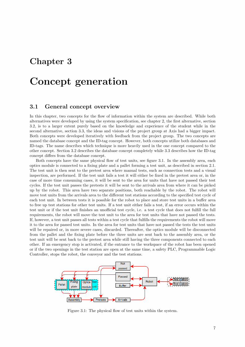
Both concepts have the same physical flow of test units, see figure 3.1. In the assembly area, eachoptics module is connected to a fixing plate and a pallet forming a test unit, as described in section 2.1.The test unit is then sent to the pretest area where manual tests, such as connection tests and a visualinspection, are performed. If the test unit fails a test it will either be fixed in the pretest area or, in thecase of more time consuming cases, it will be sent to the area for units that have not passed their testcycles. If the test unit passes the pretests it will be sent to the arrivals area from where it can be pickedup by the robot. This area have two separate positions, both reachable by the robot. The robot willmove test units from the arrivals area to the different test stations according to the specified test cycle ofeach test unit. In between tests it is possible for the robot to place and store test units in a buffer areato free up test stations for other test units. If a test unit either fails a test, if an error occurs within thetest unit or if the test unit finishes an unofficial test cycle, i.e. a test cycle that does not fulfill the fullrequirements, the robot will move the test unit to the area for test units that have not passed the tests.If, however, a test unit passes all tests within a test cycle that fulfills the requirements the robot will moveit to the area for passed test units. In the area for test units that have not passed the tests the test unitswill be repaired or, in more severe cases, discarded. Thereafter, the optics module will be disconnectedfrom the pallet and the fixing plate before the three units are sent back to the assembly area, or thetest unit will be sent back to the pretest area while still having the three components connected to eachother. If an emergency stop is activated, if the entrance to the workspace of the robot has been openedor if the two openings in the test station are open at the same time, a safety PLC, Programmable LogicController, stops the robot, the conveyor and the test stations.

Figure 3.1: The physical flow of test units within the system.

7

3.2 The database concept

The database concept is visualised in figure 3.2. The messages within the system are described in tables3.1, 3.2 and 3.3. It is recommended to follow the figure while reading this section. Each pallet stores anidentification number and the current battery level on an ID-tag. The pallet updates the stored batterylevel at a certain frequency. Each fixing plate and optics module stores an identification number and ashared type number on ID-tags.

3.2.1 Preparation of the test units

In the assembly area, the battery level of the pallet is read to ensure the pallet is fit for use. Theidentification numbers of the pallet, fixing plate, and optics module are read, paired together, and savedto a secondary database, a database used only for this system which is quicker to access than themain database. The type number is read and sent with a request to the main database which in turnprovides the assembly area with the test definition for the selected type number. The test definitiondescribes all possible tests that the specified type can undertake, it states whether the tests need to beperformed in a certain order or not, and it provides a standard test cycle to undertake. The operatorat the assembly area decides on a test cycle and the chosen test cycle is sent to the secondary databasealong with the identification number of the fixing plate. In case the chosen test cycle consists of a testthat is provided by a test station which is not currently active within the system, the operator will bepresented with a warning. The list of available types of test stations is received from the scheduler.The secondary database also stores a list of all the types of optics modules and their priority number inthe job scheduling. The operator can then choose to set a different priority for a specific test unit byhaving the new priority saved together with the identification number of the fixing plate in the secondarydatabase.

The assembly area also receives information regarding self tests of the test stations from the scheduler.The operator first receives a warning and later, if no action has been taken, a final notice that the teststation is unavailable until a self test has been carried out. The message consists of the type of teststation and its position in the system, making it possible for the operator to make an informed decisionof when to carry out the self test, depending on the current production flow. To carry out the self teststhe operator will load a special test unit into the system. This test unit is only used for the self testingof the test stations. Finally, the assembly area receives a connection check from the main database,the secondary database and the scheduler. If a connection is lost, the operator at the assembly area isinformed.

The test unit is then sent to the pretest area. Here the battery level of the pallet can be read sincethe information can be used while troubleshooting in case a pretest fails.

3.2.2 Arrival and buffer

In the arrivals area and the buffer area, the identification number and type number of the fixing plate areread. This information is sent to the scheduler together with the position of the test unit, determinedby proximity sensors. If a proximity sensor in one of the areas is experiencing an error, that informationwill be shared with the scheduler. Finally, the scheduler will also receive a connection check from bothareas.

When receiving an identification number and type number of a fixing plate from the arrival area, thescheduler sends these in a request to the secondary database that returns the earlier stored test cycle, thepriority number for that type number and, if applicable, a specific priority number for that identificationnumber as well as the estimated times in each test station within the test cycle.

8

3.2.3 Testing

For every test that is performed the scheduler will send the time duration to the secondary databasetogether with the type number of the fixing plate and the type number of the test station where thetest was carried out. If the estimated time and the actual times differ above a certain threshold thescheduler will request this list of test times for a given type of fixing plate and test station, recalculatethe estimated time, and then send the new estimation to the secondary database for storage. To enablethe possibility to share the time estimations between sites, the main database can send a request for thetime estimate for a given type of test unit and test station. The main database can also send an updatedtime estimation for a given type of test unit and test station to the secondary database. Additionally,the main database can delete types of test units and test stations from the secondary database whenthe models have become deprecated. The secondary database has a connection check from the maindatabase. If this connection is lost, the secondary database informs the scheduler. Furthermore, thescheduler has a connection check from the secondary database.

The testing stations have different configuration angles for different types of test units. To be ableto take this into account in the planning, the scheduler requests the configuration angle for each type oftest station and test unit as well as the angular velocity when changing configuration angle in each typeof test station.

When a test station is being connected to the system it sends its type number, position and currentconfiguration angle to the scheduler. If there already is a test unit in the test station at this point itwill also send the identification number of the fixing plate and the type number of the test unit. Thetest stations will also send a request, containing their type number, to the main database to receivethe correct configuration angles for each type of test unit. During the planning phase, the schedulersends notices to the test stations telling the type of the next test unit that is planned for the test station,allowing the test station to configure accordingly. The notice also consists of a variable that tells whetherthe test station is the last in the test cycle or not and the identification number of the fixing plate. Theidentification number is used here to ensure that the received information concerns the same test unitas the one later received at the test station. If the test station is the last one in the test cycle it turnsoff the pallet after the test has been finished to save battery power.

When a test station receives a test unit it reads the identification numbers of the pallet, fixing plateand optics module as well as the battery level of the pallet and the type number of the test unit. Thetest station sends the identification number of the optics module to the main database as a request toreceive any potential parameters derived in earlier tests. After a test has been carried out the test stationinforms the scheduler by sending the type number of the test station, the identification number of thefixing plate, the basic result, i.e. failed, passed, or error, the battery level of the pallet, and the timeduration of the test. The test station also sends the three identification numbers and the type of thetest unit, the battery level of the pallet, the identification number and position of the test station, thetime duration of the test, any potential parameters needed for tests further down the test cycle, andthe detailed result of the test to the main database for storage. Furthermore, the test stations informthe scheduler if they are experiencing an error, if the connection between the main database and a teststation is lost, and if the front opening, where the robot enters, or the back opening, used for maintenancework, has been opened. The test stations also inform the scheduler when they are in need of a self test.These messages are not only forwarded to the assembly area, as described earlier in this section, but alsoto the control panel.

9

3.2.4 Visualizations and statistics

For visualisation purposes, the control panel receives the current queue within the system, the progressof the individual test units within the system, the latest reading of the battery level of the pallet foreach test unit within the system and the estimated remaining time for each test unit within the systemfrom the scheduler. The test units are identified using the identification number of the fixing plate.Additionally, the scheduler provides the control panel with the average utilization factor of the robotsand the test stations as well as the average waiting time for the different types of test units. To changethe priority number of different types of test units, the operator can request a list of the current prioritiesfrom the secondary database through the control panel. Thereafter the operator can send a new priorityfor a specific type of test unit back to the secondary database. To notify the operator regarding errorsthrough the control panel, the scheduler sends one message to signal a connection error between twonodes and one message to signal an error within a node, for example a lost connection between a teststation and the scheduler or an internal error in a test station. The control panel also has a connectioncheck from the scheduler. To disconnect a test station from the system the operator sends a request fromthe control panel to the scheduler. The request consists of the position of the test station the operatorwant to access. The scheduler will replan accordingly and send a deactivation message to the test stationin question. Thereafter, the scheduler will send a confirmation back to the control panel, saying thatthe access has been granted. When the operator wants to activate a test station or any node that haspreviously been excluded from the planning due to an error, for example a certain position in the buffer,the operator sends an activation message through the control panel to the scheduler. The scheduler willthen replan accordingly and, in case the node to be activated is a test station, send an activation messageto that test station.

The scheduler is not only providing the control panel with the average utilization factor of the robotsand the test stations as well as the average waiting time for the different types of test units, but theinformation is also sent to the main database for storage. The scheduler also provides the main databasewith error logging, logging of emergency stops of the system, and logging of replanning situations dueto test units within the system being moved by operators. As other connections, the scheduler has aconnection check from the main database.

3.2.5 Safety

When an emergency stop has been activated, the entrance to the workspace of the robot has been opened,or both the front and back opening of a test station has been opened, the Safety PLC shuts down theconveyor, the robot and the test stations as well as informs the scheduler of what triggered the event.This information is forwarded to the control panel. Once the emergency stop, entrance or opening hasbeen restored, the operator can start the system from the control panel again. The exact procedure ofhow to restore these events, which is needed to comply with safety regulations, are not described withinthis thesis.

3.2.6 The robot

To move test units from one position in the system to another, the robot receives commands from thescheduler. The scheduler will tell the robot to either pick a test unit at a certain position, to place atest unit at a certain position, or to go to a certain position without picking or placing a test unit. Thescheduler can also command the robot to stop in the middle of one of these actions and the robot willinform the scheduler if the action is successful. To know the initial state of the robot, the robot informsthe scheduler if it has a test unit in its gripper or not. Furthermore, the scheduler has a connection checkfrom the robot. To avoid collisions when placing a test unit in the area for passed units or the area forunits that have not passed the tests, these areas send a message to the robot telling whether the placingarea is occupied or not.

10

3.2.7 Exiting the system

When a test unit arrives to the area for passed units or the area for units that have not passed theirtests, the three identification numbers of the test unit are read. In the area of units that have not passedtheir tests the identification number of the fixing plate is compared to the corresponding identificationnumber sent from the scheduler together with the basic result of that test unit. The basic result isused to distinguish between units that have failed their tests, units that have experienced an error andunits that have completed an unofficial test cycle. Both areas use the identification number of the opticsmodule in a request to the main database to receive the detailed result. The detailed result is used fortroubleshooting failed test units and for manual verification of the result, a feature often appreciated byoperators. As a final verification, the identification number of the fixing plate is sent to the secondarydatabase, which returns the three identification number that were paired with it in the assembly area.These numbers should still be the same. Units that have not passed their tests are either sent back tothe pretest area or the assembly area. Pallets and fixing plates from units that have passed their testsare sent back to the assembly area. When units are sent back to the assembly area, from either of thetwo areas, the pairing of the three identification numbers are deleted from the secondary database. It isnot mandatory to detach the pallet from the fixing plate when sending the units back to the assemblyarea.

11

Figure 3.2: Flow of information within the database concept. Main power switch not included.

12

Message Descriptionaccess granted A test station can now be manipulated manually.activate Activate a test station or position in the buffer or arrivals area.activate deactivate Activate or deactivate a test station.activated Signals an activated emergency stop.avg wait time The average waiting time for each type of test unit.battery p The battery level of the pallet.config angle The configuration angle of a test station.config dangle The angular velocity when changing configuration angle.connected as mdb Connection check from the main database to the assembly area.connected as s Connection check from the scheduler to the assembly area.connected as sdb Connection check from the secondary database to the assembly area.connected cp s Connection check from the scheduler to the control panel.connected s ar Connection check from the arrivals area to the scheduler.connected s b Connection check from the buffer to the scheduler.connected s mdb Connection check from the main database to the scheduler.connected s npa Connection check from the not passed area to the scheduler.connected s r Connection check from the robot area to the scheduler.connected s sdb Connection check from the secondary database to the scheduler.connected s ts Connection check from a test station to the scheduler.connected sdb mdb Connection check from the main database to the secondary database.connected ts mdb Connection check from the main database to a test station.connection error Signals a connection error between two subsystems.delete ids Delete the paired identification numbers.delete ts Delete a type of test station from memory.delete tu Delete a type of test unit from memory.error Signals an error at a test station, in the arrivals area, or in the buffer.error logging Logging the errors that have occurred.get ids Get the stored paired identification numbers.got to Command the robot to go to a specific position.gripped unit States whether the robot is holding a test unit or not.id fp The identification number of the fixing plate.id om The identification number of the optics module.id om paired The identification number of connected optics module.id p The identification number of the pallet.id p paired The identification number of connected pallet.last ts States whether a test station is the last one in a test cycle or not.occupied npa States whether the not passed area is occupied or not.occupied pa States whether the passed area is occupied or not.open States whether the entrance to the robot’s workspace is open or not.open back States whether the back of a test station is open or not.open front States whether the front of a test station is open or not.param Parameters derived during a test.param list A list of all parameters derived for a specific optics module.pick Command the robot to pick a test unit at a specific position.place Command the robot to place a test unit at a specific position.pos A position in the system.pos ar A position in the arrivals area.pos b A position in the buffer.pos ts A position of a test station.prio The prioritization number for a type of test unit.prio The prioritization number for a specific test unit.prio spec The prioritization number for a specific test unit.progress The performed and remaining test for each test unit in the system.queue The currently planned schedule.

� Only in the database concept� Only in the ID-tag concept

Table 3.1: Description of the messages within the two concepts, part 1.

13

Message Descriptionremaining time est The estimation of the remaining time in the system for a test unit.replan logging Logging the replanning that have occurred due to unexpected movements of test units.request access Request access to manipulate a test station.request config Request the configuration angle and angular velocity, for each type of test station and test unit.request prio Request the prioritization number for each type of test unit.result basic The basic result of a test, i.e. passed, failed, or error.result basic list A list of the basic results from all tests for a test unit.result detail All details concerning a test result for a test unit.self test now Indicates that a self test of a test station should be performed now.self test warm Indicates that a self test of a test station should be performed soon.start Restart the system after an emergency stop.stop Commands the robot, the test stations and the conveyor to stop.stop logging Logging the emergency stops that have occurred.stopped States that the system has been stopped due to a safety violation at a certain position.success States whether the action of the robot was successful or not.test cycle The chosen test cycle for a specific test unit.test def A definition of the possible test cycles for a specific type of test unit.test time The time duration of a test.test time list A list of all test times for a type of test unit and test station.time est The estimation of the test time for a type of test unit and test station.type ts The type number of a test station.type ts active list A list of all types of test stations that are currently active.type tu The type number of a test unit.utilization The utilization factors of the robot and the test stations.

� Only in the database concept� Only in the ID-tag concept

Table 3.2: Description of the messages within the two concepts, part 2.

Message extension Description↔ A list of paired up variables.= None Only included if currently available.

Table 3.3: Description of the message extensions within the two concepts.

14

3.3 The ID-tag concept

It is recommended to follow figure 3.3 while reading this section. As for the database concept, themessages within the system are described in tables 3.1, 3.2 and 3.3. The fundamental design of theID-tag concept is to a large extent equal to the design of the database concept, see section 3.2. However,the features that makes the ID-tag concept differ from the database concept are described in this section.In this concept there is no secondary database. Instead, additional information is stored on the fixingplate. This additional information consists of the identification numbers of the paired pallet and opticsmodule, the chosen test cycle, the chosen priority number as well as a list of the basic results.

In the assembly area, the test cycle, priority number and identification number of the paired palletand optics module are written to the fixing plate instead of stored in a secondary database. The schedulerreceives the test cycle and priority number directly from the arrivals area, buffer area, or test stations,the later two in case there is already a test unit in the buffer area or in a test station when the system isactivated. The basic result from each test station is both sent to the scheduler and written to the fixingplate. Like this, the area for units that have not passed their tests can directly read the basic resultsfrom the test unit instead of receiving it from the scheduler. Similarly, both the area for units that havepassed their tests and the area for the units that have not passed their tests can read the identificationnumber of the paired pallet and the paired optics module and thereafter delete them instead of contactinga secondary database. Here, the basic result also has to be deleted from the test unit before the fixingplate enters the system again.

Since this concept does not include a secondary database the management of time estimations for thetests in the different types of test stations need to be solved differently in this concept compared to thedatabase concept. It was chosen to use the main database for this. The scheduler sends a request withthe type of test unit to the main database. The response from the database consists of the estimatedtimes for each type test station for that type of test unit. In case the actual times differ above a certainthreshold the scheduler will request a list of test times for a given type of test unit and test station,recalculate the estimated time, and then send the new estimation to the database for storage. Since thetest times are included in the result message from the test stations to the main database, the databasealready has access to those.

Additionally, this concept does not include standard priorities for the different types of optics modulessince this feature too was enabled using the secondary database in the database concept. Instead, thepriority that is chosen for the first optics module of each type since startup at the assembly area is usedas a standard value for that type until it is changed or until the system has been shut down.

The rest of the concept design is identical between the two concepts, i.e. the difference is whether touse a secondary database or to write more information to the test units themselves.

15

Figure 3.3: Flow of information within the ID-tag concept. Main power switch not included.

16

3.4 Summary of the communication channels and the essentialhardware

This section summarizes a high level overview of the necessary communication channels and hardware forthe flow of information within the two concepts. Details such as recommending specific products or brandsare not covered. Instead the focus is on general functionality which leaves the future implementationopen for adjustments to fit in with Axis’s other systems, potential contracts with specific resellers, thedesires of the company to be hired for the system integration and any future changes of the system.However, the components that are eventually chosen need to comply with the description in this section.The components that are necessary for the conveyor, for performing the different tests in the test stationsand in the pretest area as well as the tools required for the physical assembly and dismantling is notincluded. For a summary in the form of a table, see table 3.4 for the essential hardware and table 3.5for the communication channels.

It should be possible to read stored information from the pallets, fixing plates and optics modules. Inthe ID-tag concept, it should also be possible to overwrite the information on the fixing plate. Contactlessdata transfer would simplify this automatic procedure. For the pallet and fixing plate, RFID-tags canbe used. To lower the cost of the product, the optics modules can use QR-codes instead. Additionally,it should be possible to measure the remaining battery power of the pallet. This can be done by havingthe pallet itself update the stored battery power on its RFID-tag at a certain rate.

In both concepts, the assembly area needs to read for the information stored on the test units. Inthe ID-tag concept, writing functionality is also needed. When it comes to communication, the assemblyarea needs to have a communication channel to and from the main database and from the scheduler. Inthe database concept communication to and from the secondary database is also needed. To visualizethe received data and then manipulate it before it is transmitted, an HMI, Human Machine Interface,is needed in this area. Next up is the pretest area. In both concepts, this area only needs to read theremaining battery power of the pallet and present it on an HMI. If the assembly area and pretest areais constructed together as one area, they could share the same hardware.

The arrivals area needs a reader for the information stored on the fixing plate. It also needs oneproximity sensor for each position within the area. The data from the proximity sensors needs to beprocessed and sent together with information from the fixing plate to the scheduler.

The robot not only needs the hardware and software necessary to run, but also a proximity sensorin its gripper and a communication channel to and from the scheduler. Furthermore, the robot needsto receive data from the safety PLC, the area for passed units and the area for units that did not pass.These three communication channels can be more simplistic compared to the communication channelbetween, for example, the robot and the scheduler, since this information consist of booleans, i.e. each ofthese messages can be represented by a signal that is either high or low, rather than more complex datastructures. The area for units that passed and the area for units that did not pass both need to read theinformation on the pallet, fixing plate and optics module. In the ID-tag concept, the ability to write newinformation to the fixing plate is also needed. Furthermore, the areas need communication to and fromthe main database. In the database concept, the area for units that did not pass needs communicationto and from the scheduler and both the areas need communication to and from the secondary database.Additionally, both areas need a proximity sensor and an HMI, the latter for visualizing the results of thetest units.

Continuing with the buffer, this area needs a reader for the information on the fixing plate and aproximity sensor for each position within the area. The data from the proximity sensors needs to beprocessed and sent together with information from the fixing plate to the scheduler.

The control panel needs a communication channel to and from the scheduler. In the database concept,it also needs a communication channel to and from the secondary database. Additionally, as the namesuggests, this area needs an HMI to visualize and manipulate the information.

Moving on to the test stations. The test stations need to read the information from not only thefixing plate but also the pallet and optics module. In the ID-tag concept, the ability to write informationto the fixing plate is also needed. When it comes to communication channels, the test stations needchannels to and from the main database and the scheduler. Additionally, the test stations communicatesto and from the safety PLC, however, this communication can be more simplistic since the informationconsist of booleans, a signal that is either high or low, rather than more complex data structures.

17

Additionally to the robot and the test stations, the safety PLC also needs communication channelsto the scheduler and the conveyor as well as communication channels from the entrance to the robot’sworkspace and from the emergency stops in the system. Here, all communication channels but thecommunication channel to the scheduler can be of a more simplistic nature since, again, the informationconsists of booleans, a signal that is either high or low, rather than more complex data structures.The communication channels of the scheduler and the main and secondary database have already beendescribed. The secondary database is only included in the database concept. This database can either becompletely separated from Axis’s main database management system or integrated within that system.

The communication channels that have been described as more simplistic in this section can beimplemented using I/O-communication. In case a signal is lost, a safe state should be assumed. Forproximity sensors, the safe state is to assume that the position is occupied. For safety messages used forshutting down the system, the safe state is to assume that the system should be shut down. The restof the communication channels uses more complex data structures which require a higher bandwidth.These channels should include a verification of the status of the channel, i.e. if the channel is workingas intended or not. These communication channels could be implemented using for example Ethernet.

As stated in chapter 2, all proximity sensors should include redundancy for increased reliability.Shawn Frayne [3] describes four common types of proximity sensors: IR-sensors, ultrasonic sensors,capacitive sensors and inductive sensors. The inductive sensor can only sense metal, it has a shortsensing range, it is suitable for harsh environments and it is in general the cheapest sensor out of thesefour. The three other sensors that are mentioned have the advantage that they can also sense othertypes of materials. Additionally, ultrasonic sensors and IR-sensors have a longer sensing range. However,ultrasonic sensors work best when detecting flat surfaces and IR-sensors are sensitive to, for example,dust blocking the beam of light [3]. In this system, all proximity sensors senses whether a test unit ispresent or not at a specific location. The shape and material of the test units can be adapted to fit withthe selected type of sensor, for example the test unit can either be made out of metal or have a metalplate attached to it if this is necessary for the selected type of proximity sensor. The system can also bedesigned so that the test units are being placed right by the sensor, meaning that a long sensing rangeis not required. The system will be working in an industrial environment but since dust can cause issuesfor the optics modules, the cleanliness of the working environment have certain requirements. Takingall this into account, inductive sensors are recommended. They comply with the requirements of thesystem while at the same time, in general, being cheaper than the three other types of sensors that arediscussed.

18

Subsystem Hardware

PalletsRFID-tag, RWRFID-readerMCU

Fixing platesRFID-tag, WORMRFID-tag, RW

Optics modules QR-code

Assembly

RFID-readerQR-readerMCUHMI

PretestsRFID-readerMCUHMI

Arrivals2 RFID-readers2 inductive sensorsMCU

Buffer1 RFID-reader per pos.1 inductive sensor per pos.MCU

Passed

RFID-readerQR-readerInductive sensorMCUHMI

Not passed

RFID-readerQR-readerInductive sensorMCUHMI

Robot

Industrial robotRobot controllerGripperInductive sensor

Test stations2 RFID-readersQR-readerMCU

Control panelMCUHMI

Safety PLC Safety PLCScheduler PLC

Main databaseDatabaseDBMSDatabase

Secondary databaseDBMS

� Only in the database concept� Only in the ID-tag concept

Table 3.4: A summary of the essential hardware for each subsystem.

19

Subsystem Ethernet com. with Input from Output to RFID/QR read from RFID write to

AssemblyScheduler Pallet Fixing plateMain database Fixing plateSecondary database Optics module

PretestsArrivals Scheduler Fixing plateBuffer Scheduler Fixing plate

PassedMain database Robot Pallet Fixing plateSecondary database Fixing plate

Optics module

Not passedMain database Robot Pallet Fixing plateSecondary database Fixing plateScheduler Optics module

RobotScheduler Passed

Not passedSafety PLC

Test stationsScheduler Safety PLC Safety PLC Pallet Fixing plateMain database Fixing plate

Optics module

Control panelSchedulerSecondary database

Safety PLCScheduler Test stations Test stations

Emergency stops RobotEntrance Conveyor

Scheduler

AssemblyArrivalsBufferNot passed

RobotTest stationsControl panelSafety PLCMain databaseSecondary database

Main database

AssemblyPassedNot passedTest stationsSchedulerSecondary databaseAssemblyPassedNot passedControl panelScheduler

Secondary database

Main database

� Only in the database concept� Only in the ID-tag concept

Table 3.5: A summary of the communication between the different subsystems.

20

3.5 Comparison of the concepts

Both concepts to a large extent offer the same functionality in the form of capabilities, time efficiencyand the available information at each area. The only exception to this is the handling of estimated testtimes and standardized priorities.

In the database concept, estimated test times are accessed and updated through the secondarydatabase while in the ID-tag concept they are accessed and updated through the main database. Dueto this, the process is slower in the ID-tag concept compared to in the database concept. However, thetime estimations for a type of test unit only need to be accessed the first time that type of test unit isintroduced to the system since startup and updates are only performed when the estimated times andactual times have a difference that is above a certain threshold.

In the database concept, a standard priority value for each type of optics module is stored in thesecondary database and can be changed using the control panel. In the ID-tag concept, the standardpriorities are not stored after the system has been shut down. Instead, the priority that is chosen for thefirst optics module of each type since startup at the assembly area is used as a standard value for thattype until it is changed or until the system has been shut down.

What differs more is the implementation. The ID-tag concept uses fewer communication channelssince more information is transferred with the test units. Additionally, the database concept uses asecondary database that results in a more complex database management system compared to the ID-tag concept. On the other hand, the ID-tag concept puts a higher demand on the hardware that is usedto store information on the fixing plates since, in this concept, this information is being overwrittenseveral times during each cycle in the system and, compared to the database concept, more informationis stored.

Another aspect is the potential for future updates and expansions of the system. Here the complexityof the database concept provides an advantage over the ID-tag concept. Since more areas are connectedin the database concept, more complex features can be added without updating the hardware. However,it is also an option to include these connections in the ID-tag concept, without utilizing them in the firstversion of the system, to enable future usage through software updates.

Taking just this into account, the ID-tag concept would be recommended for a future implementationsince it offers similar capabilities with a system design that is less complex. However, when discussingthe two concepts with the team at Axis, the team conveyed that the structure of the database concept ismore in line with their current expertise than the ID-tag concept. It was estimated that the advantages ofthe ID-tag concept are not significant enough to overlook this aspect and therefore the database conceptis recommended for a future implementation.

21

22

Chapter 4

Job shop scheduling

In this chapter, a job shop scheduling method for the system is derived and simulated. First, in section4.1, a scheduling model for the system is defined, in section 4.2, theories and methods regarding jobshop scheduling are described and in section 4.3, the theories are applied on the system concerned inthis thesis.

4.1 Scheduling model

In the system for this project, test units, in regards of scheduling referred to as jobs, ji, arrives to thearrivals area, an input buffer, B0, with the size of two. The jobs will then go through a defined set oftest stations with the help of a robot. In which order a certain job should go should go through thespecified test stations can be either specified, chosen freely or partly specified. Both the robot and thetest stations are here referred to as machines, M0 being the robot and M1 to Mn being the test stations.The time duration for a job, ji, in a test station, Mk, i.e. the processing time, can be referred to aspMkji

. The system also includes a buffer, B1, where jobs can be placed by the robot to free up teststations or the input buffer. In this project, the buffer will have a limited size which can be varied inbetween simulations. Once jobs are finished or cancelled, due to errors or failures, they leave the systemthrough one of the output areas, with the help of the robot. Each of the test stations, M1 to Mn, has acertain setup time when changing from one type of job to another. This is due to different jobs requiringdifferent configuration angles in the test stations. The setup can be performed as soon as the previousjob has been processed, i.e. the previous job does not have to leave the machine before the setup canbegin. The setup time between jobs, ji and jl, in a test station, Mk, can be referred to as sMkjijl

. Thereis also a setup time for the robot, the time to get from its current position to the machine or bufferwhere a job will be collected. This setup can also be performed beforehand, i.e. before the job is readyin a machine. The setup time for the robot when going from, for example Bi to Mk, can be referredto as sM0BiMk

. For the robot, an equivalent processing time can be defined as, in the cases where thepick-up position is a machine, the time it takes to enter the machine, the time it takes to collect ajob, deliver it to its next location and, in the cases where the drop-off position is a machine, have therobot exit the machine. If a job is for example collected as Mk and will be placed at Bi, the processingtime can be referred to as pM0MkBi

. In addition to the machine and buffers, the robot have three morepositions: the two output areas, referred to as Oi and its home position, referred to as H. In the caseswhere the robot is starting in another position than the ones described here, the robot will go to thehome position and initialize the scheduling from there. The scheduler should be flexible when it comesto introduction of more test stations, deactivation of test stations, jobs in unpredicted initial startingpositions and cancellations of jobs. All specified time durations will be approximated, i.e. the true timesmay deviate from the approximations. The described model is visualised in figure 4.1.

In this system, jobs do not have a specified due date, it should however be possible to give differentjobs different priorities. The main objective is to maximize the throughput of the system while no jobsget stuck in the system waiting.

23

Figure 4.1: The scheduling model.

4.2 Job shop scheduling theory

For static scheduling problems consisting of one to two machines and n jobs, for cases with n machinesand two jobs and, under certain conditions, for problems consisting of three machines and n jobs as wellas for a limited number of special cases of more complex systems, general methods have been derived.However, optimizing the general case of more complex systems are NP-hard [10]. A problem is NP if itis solvable in nondeterministic polynomial time and if a problem is NP-hard it means that an algorithmfor solving it can be translated into one that solves any other NP-problem [13]. None of the cases thathave a general method derived matches the dynamic model described in section 4.1.

For dynamic cases like this, with new job arrivals, machine breakdowns and job cancellations, Wanget al. [12] present a framework for how to handle dynamic job shop scheduling. They divide dynamicscheduling into four areas: methods, strategies, policies and approaches, see figure 4.2.

Figure 4.2: The scheduling framework presented by Wang et al. [12].

24

The methods are split up into two categories, schedule generation and schedule repair. For schedulegeneration three methods are mentioned, no schedule, nominal schedule and robust schedule. With anominal schedule, the initial schedule is created without real time events, such as job cancellation, takeninto account. With a robust schedule, the initial schedule builds upon predictions of upcoming real timeevents. In the final case, no schedule, no initial schedule is generated. Instead commands are chosenin real time. Wang et al. also name three alternatives when it comes to schedule repair, right-shiftrescheduling, complete rescheduling and partial rescheduling. In right-shift rescheduling, the content ofthe schedule is pushed forward in time to allow for unexpected time delays. In complete rescheduling, thewhole schedule is reevaluated once a real time events affect the schedule. Finally, in partial rescheduling,only the operations that are affected by a real time event are reevaluated [12].

Wang et al. describe three different strategies. Completely reactive scheduling, predictive reactivescheduling and robust pro-active scheduling. In completely reactive scheduling the scheduling is per-formed in real time without predictions. In predictive reactive scheduling, a schedule is generated bypredicting the outcome of a system. The schedule is then adapted according to real time events. In ro-bust pro-active scheduling, the effect of system disturbances and performances are predicted beforehandto generate a schedule in advance [12].

Furthermore, Wang et al. present three policies for implementing the strategies: periodic reschedul-ing, event-driven rescheduling and hybrid rescheduling. All three policies take real time events intoaccount, however, periodic rescheduling takes events into account only at a specific rate, event-drivenrescheduling handles the events as they occur and in hybrid rescheduling the rescheduling is done peri-odically but it is only carried out in case a real time event has occurred [12].

Finally, Wang et al. bring up three approaches, heuristic rules, classical optimization and artificialintelligence approaches [12]. These require a more substantial review and are therefore described in moredetail in the upcoming subsections, namely subsection 4.2.1, 4.2.2 and 4.2.3.

4.2.1 Heuristic rules

Heuristic rules, also known as dispatching rules, are prioritization rules based on attributes of jobs,machines and time. In each step when choosing a job to process, the job with the highest resultingpriority according to the rule is chosen. Depending on which factors the objective is related to, factorssuch as maximum lateness, variation in waiting time, workload balancing, throughput and so on, differentrules tend to be more effective. However, no guarantees are given. [5]

Michael L. Pinedo [5] describes 12 standardized heuristic rules and for which objectives they tend tobe the most effective.

• The earliest release date first rule, the job that arrived to the system first is chosen first, tends tominimize the variation in the waiting time.

• The earliest due date rule, the job with the earliest due date is chosen first, and the minimum slackrule, the job with the smallest difference between the time until the due date and the processingtime is chosen first, tend to minimize the maximum lateness.

• The longest processing time first rule where, as the name suggests, the job with the longest process-ing time is chosen first, tend to balance the workload over the different machines to the maximumin cases were machines work in parallel.

• The shortest processing time first rule tends to minimize the sum of the completion times of thejobs.

• By modifying the shortest processing time first rule by introducing weights to the different jobs, theweighted shorted processing time first rule tends to minimize the weighted sum of the completiontimes.

• When the queue behind each available job is known, the critical path rule, where the job that isin first place of the queue with the highest sum of processing times is chosen first, and the largestnumber of successors rule, the job that has the highest number of jobs in queue behind it is chosenfirst, tend to minimize the makespan of the jobs, i.e. the time duration that each job spends withinthe system.

25

• The shortest setup time first rule, the job that requires the shortest setup time is chosen, and theleast flexible job first rule, where the job that has the lowest number of alternative machines tochose from is chosen first, tend to minimize the makespan of the jobs and maximize throughput ofthe system.

• The shortest queue at the next operation rule, the job that has the shortest queue in between leavingthe upcoming machine and entering the next one is chosen first, tends to minimize the machineidleness.

• Finally, the service in random order rule, where jobs are chosen at random, is the solution thattends to minimize the complexity of the implementation.

However, in practise the sought objective could be a time dependent combination of several factors.Pinedo [5] explains that several heuristic rules can be combined into more complex rules by applyingscaling functions to a combination of the standardized heuristic rules. These rules have to be determinedby the developer to fit the needs of the specific system. Experience is helpful when designing the rulesbut simulations are needed to fully validate them [5].

4.2.2 Classical optimization

When solving the scheduling problem by using classical optimization, dynamic programming and branchand bound methods are the most commonly used techniques [6].

Michael L. Pinedo [6] explains that the idea behind dynamic programming is to divide the probleminto subproblems and calculate the optimal solution for each subproblem. When there are more thanone way of dividing the problem, each possible way is explored. The solutions are then combined toform the main problem and an optimal solution for the main problem is calculated. Pinedo concretizesdynamic programming for the case of dynamic job shop scheduling. Each job is given a cost. Thecost depends on the time when the job is finished and can include different scaling factors for differentjobs. The sum of the costs for all jobs forms the full objective that should be minimized to achieve theoptimal solution. The jobs that are available for processing are split into subgroups, each with a fixednumber of jobs. When the total number of jobs is a prime number, one single group can consist of fewerjobs than the others. Dynamic programming has two different approaches, forward and backward. Inforward dynamic programming, one subgroup is chosen as the first one to process. By iterating throughall different combinations, the optimal order for the first subgroup, when it is processed first, is found.Then, another subgroup is chosen as the second subgroup to be processed and the optimal order for thatsubgroup, when processed as the second subgroup, is found in the same way as for the first subgroup.This goes on until an optimal order has been derived within each subgroup, given a set processing orderof the subgroups. If one subgroup has fewer jobs than the other, this subgroup should be processedlast. This process is repeated for every possible order of the subgroups. As a final step, this processis repeated for every possible formation of subgroups of the previously chosen fixed size. Once this hasbeen done, the solution with the lowest total cost is the optimal processing order. Backward dynamicprogramming works similarly to forward dynamic programming. The only difference is that instead offirst choosing the first subgroup to be processed and work from there, the last subgroup to be processedis chosen first and the method continues by working towards the first subgroup to be processed. If njobs shall be processed in one machine, it can be shown that the total number of evaluations needed tosolve the problem with this method are O(2n) [6]. A visualization of forward dynamic programming forjob scheduling is shown in figure 4.3.

26

Figure 4.3: A visualization of forward dynamic programming for job scheduling.

Patrick Winston, instructor at MIT, explains the branch and bound method by applying it to anexample where the shortest path between two nodes in a map is sought [14]. The paths between thenodes in the map each have a positive, nonzero, cost assigned to them. A search tree is built with thestarting node as the root. Each possible path leading to new nodes from the root are explored, formingbranches in the search tree. Once all paths that are leading out of the root have been explored, thealgorithm steps down one layer in the tree and starts exploring all paths leading out of the second layerof nodes, starting with the node that has the lowest cumulative sum of costs in its path from the root.One node at a time, the algorithm continues to explore paths leading out of the nodes, always startingwith the node with the least cumulative sum of costs, until the end node has been reached and no nodewith unexplored paths and a shorter cumulative sum of costs than the full way to the goal exists. Byadding what is called an extended list to the branch and bound method, the algorithm keeps track ofwhich nodes it has reached previously and what the lowest cumulative sum of costs from the root to eachnode is. If the algorithm comes back to a node it has already visited through another branch, only thebranch with the lowest cumulative sum of costs will be expanded further [14]. The method is visualizedwith an example in figure 4.4.

27

Figure 4.4: A visualization of the branch and bound method with an extended list. The optimal pathfrom A to F in the map to the left in the figure is sought.

Furthermore, Winston [14] describes that in cases where the remaining distance from a node to thegoal can be given a lower bound before the branches leading out from that node have been explored, thealgorithm can be improved further. Instead of extending the node with the lowest cumulative sum ofcosts next, the node where the sum of the cumulative sum of costs and the lower bound of the remainingdistance is the lowest, is extended first. When the goal node has been reached and, by taking the lowerbound of the remaining distance into account, no other branch can reach the goal at a lower cost, theoptimal path has been found [14].

The branch and bound method used together with an extended list and with utilization of lowerbounds on the remaining distance from each node forms a method known as A*, pronounced A-star.Russell and Norvig [11] state that the time complexity of A* depends on the accuracy of the set lowerbound, i.e. how close the lower bound is to the actual cost. However, for most heuristics in practicaluse, the time complexity is exponential in the solution depth of the search tree. The main drawback ofA* is however not the time complexity, but rather the space complexity since all generated nodes arestored in memory [11].

The explanation of branch and bound and A* given by Winston is based on finding the optimal routebetween two nodes in a map [14]. For the purpose of this thesis, the problem needs to be reformulatedto fit with job scheduling, a problem that has different characteristics depending on the application.For some special cases, the adaptation of the algorithm has received considerable attention in previousstudies. One example of such special cases is the case with one machine and several jobs that each havea release date and a due date. The adaptations of the algorithm for this problem has been described byPinedo [7].

28

4.2.3 Artificial intelligence approaches

The artificial intelligence techniques that are typical for solving the job scheduling problem are oftenmeta heuristic approaches, such as the genetic algorithm, tabu search, beam search, multi-agent systems,neural networks, ant colony optimization, artificial bee colony algorithm and variable neighbourhoodsearch [12]. To limit the scope of this analysis, only beam search, genetic algorithms and tabu search arecovered here.

According to Pinedo, the beam search method combines the branch and bound method with heuristicrules, see subsections 4.2.1 and 4.2.2, to eliminate the amount of branches that are being extended [8].At each level in the search tree, the nodes are evaluated and only the most promising nodes are extendedfurther. As a compromise between spending time on extending more nodes and spending time onperforming a more complex evaluation of the nodes, the evaluation process can be split up in two stages.First, a quicker evaluation is performed on all nodes at the current level. The nodes that perform thebest in this evaluation move on to the next stage. The amount of nodes that moves on to the nextstage is referred to as the filter width. In the second stage, a more time consuming evaluation methodis performed on the remaining nodes and only the nodes with the best results are extended to the nextlevel in the search tree. The amount of nodes that is further extended is refereed to as the beam width.The evaluation process consists of heuristic rules or a composition of several heuristic rules. This methoddecreases the computing time of the branch and bound method but there is no longer a guarantee thatthe found solution is optimal [8].

Genetic algorithms are also explained by Pinedo [8]. This algorithm uses some heuristic rules, seesubsection 4.2.1, to create several schedules. The generated schedules are ranked according to a selectedobjective, for example the throughput of the system or the average waiting times of the jobs etc. Thetwo schedules that performs the worst are disregarded and two new schedules are constructed by in apredefined way combining features from the two schedules that performed the best. The newly createdschedules are considered neighbors to the schedules they originated from. In the example of parallelmachines simultaneously processing a sequence of jobs each an example of a feature to combine is thesequences in different machines. The remaining schedules, that is all schedules but the two that performedthe worst, are kept the same and the ranking process starts again. This process continues for a predefinednumber of iterations before the best performing schedule is chosen. Just as for the beam search method,this method does not guarantee an optimal result [8].

Tabu search is also described by Pinedo [8]. Tabu search can be seen as a special case of geneticalgorithms. The algorithm is described in the following way. An initial schedule is generated usingsome heuristic rules. New schedules from the neighbourhood of the initial schedule are generated. Ifthe system consists of several jobs that should be processed in a single machine, the neighbourhood canbe defined as the schedules that can be generated by switching place on two adjacent jobs. Out of thenewly generated schedules, the best performing schedule according to a selected objective function iskept and the change from the initial schedule to the chosen schedule, defined by for example the twojobs that switched place in the previously mentioned example, is kept in a so called tabu list. If thegenerated schedule performs better than the initial schedule, according to the same objective function,the new schedule is also stored as the best schedule so far. The algorithm performs another iterationby generating new schedules out of the neighbourhood of the previously generated schedule, regardlessif the schedule was better than the last one or not. However, after the initial iteration the tabu listcomes into place. At each iteration, changes that are already in the tabu list may not be performedagain, meaning that schedules generated through such changes should not be considered when pickingthe best performing schedule within the neighbourhood. At each iteration the chosen change is addedto the tabu list. However, the tabu list has a limited size so at each iteration the oldest element in thelist will be deleted and it will once again be considered as a valid option. The tabu list is used so thatthe algorithm does not come back to the same local minimum over and over again. When the algorithmhas gone through a set number of iterations or when a better performing schedule has not been foundfor a certain number of iterations, the algorithm is finished and the schedule that performed the best isapplied. In more complex setups compared to the mentioned example, defining the neighbourhood of aschedule is a considerable challenge when applying the algorithm. As for the beam search method andgenetic algorithms in general, this method does not guarantee an optimal result. There are also morecomplex versions of tabu search, for example one method that uses a so called tabu tree. Instead of justsaving the tabu list and the best solution so far, nodes are generated in a tree structure, each level inthe tree being the neighbourhood of the layer above. In this way, nodes that did not seem promising atfirst can be revisited if the result from expanding an initially more promising node turns out to be lesseffective than what was anticipated at first [8].

29

4.3 Adapt the theory to the system

In this section, the framework presented in section 4.2 is applied on the system represented by the modelin section 4.1 and the demands on flexibility in the scheduling according to the system specifications inchapter 2.

Firstly, a method is decided. To maximize the efficiency of the system, a job schedule should optimallybe used. The real time events affecting the system, such as deactivated and activated machines, jobs thatfailed a test, etc. are considered as both common and unpredictable. Therefore, the schedule generationshould consist of a nominal schedule. Since a single machine, the robot, is in the central of the systemin a way that all jobs have to go through this machine when moving to another, a real time event in onepart of the system will affect the entire system. The real time events also impose new system restrictionsand goals, for example more available machines or a job being cancelled, meaning the real time eventscannot be taken care of by right-shifting the schedule. In conclusion, the schedule repair should be basedon complete rescheduling.

Secondly, a strategy is decided. As previously stated, some real time events cannot be predicted,however, there are also some predictions that can be made, namely predicting or estimating the processingtimes within the system. Taking this into account, the most appropriate strategy is to use predictivereactive scheduling.

Thirdly, a policy is decided. The real time events affecting the system, as previously stated, changethe direct restrictions and goals of the system. These events need to be considered as soon as they occur.Therefore, event driven rescheduling should be used.

Finally, the alternative approaches that were studied in subsection 4.2.1, 4.2.2 and 4.2.3. To limitthe scope of the project, it was chosen to focus on heuristic rules, the branch and bound method, A*and beam search in the implementation. These methods represent all three approach categories andfurthermore, the branch and bound method and A* have potential to be less time consuming thandynamic programming and beam search builds on a combination of branch and bound, or A*, andheuristic rules which lower the development time compared to if genetic algorithms or tabu search wereto be implemented instead.

Firstly, the method of using heuristic rules is adapted. This method does not generate a schedule,instead the actions are decided in real time. As stated in section 4.1 the jobs have no defined due dateand the system does not know about jobs that have not yet arrived to the system. Furthermore, it shouldbe possible to set different priorities for different jobs. The main objective is to maximize the throughputwhile no jobs get stuck in the system. As stated in subsection 4.2.1, the shortest setup time first rule andthe least flexible job first rule tend to maximize the throughput of the system while the earliest releasedate first rule tends to minimize the variation in waiting time. In this case, there is a considerable chancethat the jobs within the system have an equal amount of flexibility due to the possibility of adding moremachines to the system to adapt according to the flow of production. A combination of the shortestsetup time first rule, the earliest release date first rule and prioritization weights therefore have potentialto be effective in this case. However, as stated in subsection 4.2.1, no guarantees for an optimal solutioncan be given. It is not a goal to minimize the variation in waiting time but the variation should belimited to a certain level.

30

The combined heuristic rules should give a higher priority for jobs with a lower setup time and itshould be possible to assign jobs with prioritization weights. The structure of the system, see figure 4.1,shows that each move consists of going through M0 to the next location, which can be another machine.Therefore, the setup time to consider is the setup time of M0 plus any remaining setup time for theupcoming machine in case the setup has not finished once the job arrives at the machine. The process-ing time for the test stations only depend on the jobs and can therefore not be altered. However, theprocessing time for the robot, M0, depends on the chosen schedule. Therefore, a lower processing timein M0 should increase the priority. To give priority to jobs that have been in the system substantiallylonger than other jobs, the priority should increase exponentially with increased waiting time, i.e. as therelease date gets older. The suggested prioritization function for each job is shown in equation 4.1 andvisualized in figure 4.5. The structure of this equation was inspired by the apparent tardiness heuristic,which is a combination of the weighted shortest processing time first rule and the minimum slack firstrule, suggested by Pinedo as a solution for a system with one machine and several jobs [5].

Ij(t) =wj

appj + assjear(t−rj), t > rj (4.1)

wj = Prioritization weight, job j

pj = Processing time, job j

sj = Setup time, job j

rj = Release date, job j

ap = Scaling parameter, processing time

as = Scaling parameter, setup time

ar = Scaling parameter, release date

t = Time

rj

wj

appj+assj

t

I j(t

)

Ij(t) =wj

appj+assjear(t−rj), t > rj

Figure 4.5: The combined heuristic rules as a function of time.

31

Secondly, the theory of the branch and bound method and A* is adapted. In job scheduling, thegoal is not to find an optimal route between two nodes, but to find an optimal sequence for processingall of the jobs. The nodes, in subsection 4.2.2 formulated as positions in the map, can be reformulatedinto a representation of the system that describes which jobs have been processed in which machines andwhere in the system the jobs are currently located. The cost of each action, previously formulated asa distance between nodes, can be formulated as the sum of the remaining processing time for a certainjob in a certain machine and the proportion of the setup time that can not be finished before the jobis ready to enter the machine. The processing times of each test station only depend on what type ofjob that is being processed. The processing time of the robot depends on the position of the job andthe position of the next test station for that job. The setup time of the robot depends on the currentposition of the robot and the position of the job it should pick up. The setup time of the test station notonly depends on the job that is going to be processed, but also the previously processed job. Since thetest cycle defines which type of test stations each job should go through and the setup times for the teststations and the robot as well as the processing time of the robot depends on the generated schedule,the processing times of the remaining test stations for a job plus a lower bound of the processing timesin the robot can be used as a lower bound until a job is finished. Since jobs can be processed in parallel,the job with the highest lower bound gives the lower bound for finishing all jobs within the system.

This technique would find an optimal solution for processing all jobs the quickest. However, prioriti-zation on different jobs are not taken into account. To take this into account, the representation of thecost would have to be reformulated to a function dependent on not only time but also the prioritizationnumber of the involved jobs.

Finally, combining the branch and bound method or A* with the derived heuristic rule form the beamsearch method. Taking the time complexity of evaluating the heuristic rule and the limited amount ofnodes at each level into account, it was chosen not to split up the filtering into two stages. The beamwidth should be variable in the simulations.

32

Chapter 5

Simulations

Before the implementation of the simulation program could start, the purpose of it had to be established.It was discussed whether the focus should be on fully mimicking the database concept to get a completeproof of concept where the user can observe and manipulate the system in the middle of a runningsimulation or if the focus should be on simulating larger production sequences where utilization factorsand production times can be simulated in a predefined system setup. Out of these two alternatives,the latter was more in line with the needs of the company. Axis requested that the simulation programshould be written in C#. The student did not have previous experiences from C# so the workflowstarted of with an introduction to the language, focusing on general syntax, multi-threading and userinterfaces. This chapter describes the structure and capabilities of the program. Due to the size of theprogram, over 3900 lines of code with relatively long algorithms, the complete code will not be presentedin this report. Instead, the focus will be on describing the structure and algorithms in text with the helpof shorter code snippets.

5.1 General structure

Each of the different subsystems visualized in figure 3.1 plus the scheduler and secondary database,visualized in figure 3.2, were implemented as separate threads. A class that represents jobs were createdand to simulate jobs moving within the system, objects of the job class are sent between the differentthreads using channels were each channel has a reader and a writer. For example, the assembly threadhas a channel writer that sends job to the channel reader in the pretest thread. When the movement isinitialized from the receiving thread, i.e. when a job should be picked by the robot, the robot thread sendsa request to a subsystem which in turn sends a job as response. For example, the robot sends requestscontaining a position index to the test stations thread using one channel. The test stations thread thensends the job currently located in that position to the robot thread through another channel.

The communication between the threads was implemented in the same way as the movement of jobs,i.e. by sending the information in channels. To synchronize the timing between the different threads,the scheduler sends out updated time stamps to each time dependent thread throughout the course ofthe simulation.

33

5.2 Configuration

When starting the simulation, the user is presented with a graphical user interface made with windowsforms [4]. The user is requested to select a configuration file for the simulation. The simulation usesconfiguration files written in the file format TOML, Tom’s Obvious Minimal Language, [9] and anexample of a configuration file can be found in listing 5.1.

As seen in listing 5.1, the user can specify a failure rate of the pretests, that will be sent from themain thread to the pretest thread, and breakdown times for the 2 positions in the arrivals area, whichwill be sent to the arrivals thread. In this example the breakdown times are set to -1 and 3000, thisrepresents that the first position will not break but the second position will break 3000 seconds into thesimulation.

Continuing reading the file, the user can select the parameters for the heuristic rule from equation4.1 which will be sent to the scheduler thread.

Furthermore, the user defines the jobs that are going to be sent from the assembly area during thesimulation. Each defined job configuration represents an incoming rate of a certain type of jobs with aspecified test cycle and prioritization value. In this example 50 jobs of type 1 with prioritization 3 willbe sent with 180 seconds between each job starting at time 0. The test cycle consists of test stations oftype 1, 2 and 3 where type 1 should go first but the order between type 2 and 3 does not matter.

Further down in the example, the buffer is configured. The size of the buffer is decided and, similarlyto the arrivals area, a breakdown time can be set for each position in the buffer. Each position in thebuffer can also be given an initial job, a job that is located in that buffer position when the simulationsstart. The buffer configuration is not only sent to the buffer thread, the scheduler will also receive thesize of the buffer and the main thread will, during the configuration, send the prioritization value andtest cycle of any jobs initially located in the buffer to the database thread for storage.

Finally, the example shows how test stations are configured. Test stations of specified types areentered one after another in an order that corresponds to the position they are located at. Similarly tothe buffer and arrivals area, each test station has a breakdown time but also a connect time, representingwhen the test station is connected to the system and, from there on, available for usage. Furthermore,each test station is given an initial job configuration and, potentially, a job that is located within thetest station when it is connected to the system.

34

1 PretestFailureRate = 0.03

2

3 ArrivalsBreakdownTimes = [-1.0, 3000.0]

4

5 [SchedulingConfig]

6 HeuristicRuleProcessTimeScaling = 1.0

7 HeuristicRuleSetupTimeScaling = 1.0

8 HeuristicRuleReleaseDateScaling = 0.05

9

10 [[ AssemblyJobConfigs ]]

11 JobType = 1

12 TestCycleTypes = [1, 2, 3]

13 TestCycleOrderSpecification = [true , false , false]

14 NbrOfJobs = 50

15 FirstSendTime = 0.0

16 TimeBetweenSends = 180.0

17 Prio = 3

18

19 [[ BufferConfigs ]]

20 BreakdownTime = -1.0

21 [BufferConfigs.InitialJob]

22 JobType = 2

23 TestCycleTypes = [1, 3]

24 TestCycleOrderSpecification = [true , true]

25 Prio = 2

26

27 [[ BufferConfigs ]]

28 BreakdownTime = 3000.0

29 [BufferConfigs.InitialJob]

30

31 [[ TestStationConfigs ]]

32 Type = 1

33 ConnectTime = 0.0

34 BreakdownTime = 2500.0

35 TestFailureRate = 0.01

36 InitialJobTypeConfig = 1

37 [TestStationConfigs.InitialJob]

38

39 [[ TestStationConfigs ]]

40 Type = 2

41 ConnectTime = 0.0

42 BreakdownTime = -1.0

43 TestFailureRate = 0.01

44 InitialJobTypeConfig = 1

45 [TestStationConfigs.InitialJob]

46 JobType = 3

47 TestCycleTypes = [1, 3, 2]

48 TestCycleOrderSpecification = [false , false , true]

49 Prio = 2

50

51 [[ TestStationConfigs ]]

52 Type = 3

53 ConnectTime = 0.0

54 BreakdownTime = -1.0

55 TestFailureRate = 0.01

56 InitialJobTypeConfig = 1

57 [TestStationConfigs.InitialJob]

58

59 [[ TestStationConfigs ]]

60 Type = 1

61 ConnectTime = 3000.0

62 BreakdownTime = -1

63 TestFailureRate = 0.01

64 InitialJobTypeConfig = 2

65 [TestStationConfigs.InitialJob]

Listing 5.1: An example of a configuration file.

35

5.3 The assembly thread

The assembly thread receives the job configuration and sends the time when the first jobs are going to besent from the assembly area together with the amount of jobs that are sent at that time to the schedulerthread. Thereafter, the assembly area waits for an update of the time stamp from the scheduler. Whenthe time stamp matches the time when the next job is going to be sent, the assembly area gives thatjob an identification number, sends the prioritization value and test cycle to the database thread andthereafter sends the job to the pretest area. After this is done, the assembly area will also send the timewhen the next jobs are sent together with the number of jobs sent at that time to the scheduler. Thescheduler needs this information to know how the time stamp should be updated.

5.4 The pretest thread

Every time a job is received to the pretest thread, the pretest thread will perform a simulated test wherethe chance of passing is in accordance with the failure rate configuration. The job will only be sentforward to the arrivals area if it passes the pretest. Otherwise, the job is discarded. The time of apretest is set to 0, meaning that the job is sent forward at the same time stamp as it arrived to the area.The pretest thread will also send a notification to the scheduler, telling whether each carried out pretestis passed or not. This information tells the scheduler whether it should expect an arriving job or not.

5.5 The arrivals thread

When the arrivals thread receives its configuration, the potential times of breakdowns are sent to thescheduler to be used when determining the update of the time stamp. The arrivals thread receives thejobs from the pretest thread and notifies the scheduler of the arrival. This notification consists of theposition of the job, its type number and its position in the arrivals area. If there are more than two jobsin the arrivals area, jobs will be placed in a queue and the notification for that job will not be sent untilthe job has reached one of the two positions that are reachable by the robot. If a position in the arrivalsarea is set to experience a breakdown, the thread will notify the scheduler about the breakdown at thetime it occurs. Jobs will still arrive to the area but the scheduler will not be notified about these jobs,meaning that if a job arrives to that position, it will be stuck there throughout the rest of the simulation,which will be accounted for by the scheduler.

5.6 The robot thread

The robot thread receives commands from the scheduler. The commands tell the robot to pick a job froma certain position or to place a job at a certain position. When the action is completed, the robot willnotify the scheduler. The robot itself does not handle any time durations for the movements, howeverthe scheduler uses a function for calculating the time durations for each action of the robot.

5.7 The buffer thread

When the buffer has received its configuration, it will notify the scheduler of any initial jobs in the bufferand off any upcoming breakdown times. Similarly to the arrivals thread, the buffer thread will alsonotify the scheduler when a predefined breakdown occurs at a specific position within the buffer, anyjobs currently located at that position will be discarded. Whenever the buffer receives a job from therobot, it will notify the scheduler as a confirmation that the correct job has arrived. This is, however,not utilized in the scheduler but in a future update it could be used as another way of inserting simulatederrors in the system.

36

5.8 The test stations thread

A single thread handles all the test stations. When this thread receives its configuration, the connecttimes and breakdown times are forwarded to the scheduler. The test times for each job type in eachtest station are stored in the database. When the test stations thread receives its configuration, it willalso request the test times for all types of test stations included in the configuration from the databasethread. When a test station is connected, the scheduler will be informed of the type of the test station,the position, the configuration and the id and type of any initial job in the test station. Similarly tothe buffer and arrivals thread, the scheduler will also be notified when a test station is experiencing apredefined error. Before each test, the test stations thread receives information on the upcoming testfrom the scheduler, the test station in question will then prepare by changing the configuration to matchthe upcoming job type. When the job is received, the test stations thread will calculate when the testshould be finished. When the time stamp matches this time, the test stations thread notifies the schedulerwith a test result that is randomized according to the configured failure rate.

5.9 The scheduler thread

A simplified pseudo code version of the main loop of the scheduler is shown in listing 5.2. This loop isentered once the scheduler has received a complete configuration. First, the initial jobs must becomeavailable. The scheduler will check when the first event occurs, i.e. arriving jobs, connected test stations,or breakdowns, etc. The time stamp is then updated accordingly. Then the scheduler will check if therewill occur any breakdowns at this time stamp. If so, the scheduler will wait for a breakdown notification.Next up, the scheduler will check for arriving jobs, connected test stations and any initial jobs in a teststation or in the buffer. For any arriving jobs, the scheduler will request the prioritization value and testcycle from the database. If a new job type arrives for the first time, the scheduler will also request thetest times for that type of job from the database. All this is done in line 1-6 in listing 5.2. It is enclosedin a while loop since pretest failures and breakdowns can stop expected jobs from becoming available.

Then the main while loop is entered and will not be exited until the scheduling is done or has faileddue to a deadlock. The scheduler will first use the information of all available jobs and determine thebest action to take using the heuristic rule defined by equation 4.1. This function will be explainedin more detail later in this section. If no action is available, either a deadlock has been achieved or,more commonly, the scheduler needs to wait for tests to finish. Therefore, if no action is available, thescheduler will perform the steps from line 3-5 again. What was not mentioned before, since it is notrelevant until the first test has started, is that when checking for available jobs, test results are alsoreceived. If, however, an action is available the scheduler will command the robot to perform this action.

If the end position is a test station the scheduler will start by sending the information of the job tothe receiving test station. Then the scheduler will send the pick and place commands to the robot whilealso updating the time stamp with the time duration of the action. During this procedure, new eventsare also registered, again similarly to line 3-5. In cases where the end position is a test station, oncethe action has been performed, the time when the test is finished is stored. To calculate this time, thetest time is added to any remaining time duration for changing job configuration in the test station, incase the time duration for changing configuration is longer than the time duration of the action. Thejob will be marked as unavailable until a test result is received. If the end position on the other hand isthe buffer, the job will remain available and if the end position is the passed or not passed area, the jobwill be removed.

Once the action has been performed, the scheduler will once again update the time stamp and receivethe new system state. The loop then continues until there are no more jobs to handle or until a deadlockhas occurred. Once at this point, the scheduler will send the results of the simulation to the main thread.

37

1 while (No jobs available && More jobs arriving)

2 {

3 UpdateTimeStampToNextEventTime ();

4 CheckForBreakdowns ();

5 ReceiveAvailableJobsNTs ();

6 }

7

8 while ((Jobs available || Jobs being tested) && No deadlock)

9 {

10 (bestIdFp , bestStartPos ,

11 bestEndPos , bestSetupTimeRobot ,

12 bestProcessTimeRobot ,

13 bestRemainingsetupTimeTs) = GetNextActionHeuristicRule ();

14

15 if(bestStartPos == null)

16 {

17 UpdateTimeStampToNextEventTime ();

18 CheckForBreakdowns ();

19 ReceiveAvailableJobsNTs ();

20 }

21 else

22 {

23 PerformAction(bestStartPos , bestEndPos ,

24 bestIdFp , bestSetupTimeRobot ,

25 bestProcessTimeRobot ,

26 bestRemainingsetupTimeTs);

27 }

28

29 while (No jobs available && More jobs arriving)

30 {

31 UpdateTimeStampToNextEventTime ();

32 CheckForBreakdowns ();

33 ReceiveAvailableJobsNTs ();

34 }

35 }

36 SendResult ();

Listing 5.2: The main loop of the scheduler thread.

The algorithm for selecting the next action using the heuristic rule from equation 4.1 will now beexplained. The complete algorithm can be found in appendix A and a visualization of the algorithm canbe found in 5.1. The algorithm checks the available actions for each available job. Each job can eitherhave failed a test or be done with its test cycle, have only one type of test station as an option for thenext action, or have several different types of test stations as the next option.

In the first case, if the job has either failed a test or is done with its test cycle, see line 15-49 inappendix A or the upper left branch in figure 5.1, the job should be moved to the passed or not passedarea. The algorithm calculates the setup time of the robot, i.e. the time to get to the job, and theprocess time of the robot, i.e. the time it takes to move the robot to its end area. With the help ofthese values as well as the prioritization value and release time of the job and the parameters defined inthe configuration, a scheduling prioritization value is calculated using equation 4.1. If this is the highestvalue found so far, the action will be saved as the best one so far.

Continuing with the second case, when the job only have one type of test station to choose from, seeline 50-124 in appendix A or the upper middle branch in figure 5.1. The algorithm loops through eachof the connected test stations and checks if they are of the right type. For test stations of the correcttype, the algorithm checks if the test station is occupied by another job that is done with its test. Ifthis is true and no available action can be found, that is the sign of a deadlock. Therefore, the teststation in question will be stored together with the job requesting to go there so that the informationcan be used if a deadlock has occurred. Otherwise, if the test station is not occupied and it has notbeen reserved by another job to solve a deadlock, this is explained further down in the algorithm, thescheduling prioritization value is calculated in the same way as in the first case, with one exception. Ifthe job is already located at a test station of the correct type, the job will receive the highest possiblescheduling prioritization value and the algorithm will return the action. This is because such an actionwould take zero time and no other action that requires manipulation by the robot can achieve a higherscheduling priority.

38

Finally the third case, when the test cycle of the job allows for several different types of test stationsnext, see line 125-223 in appendix A or the upper right branch in figure 5.1. Here, the algorithm firstchecks how many of the upcoming tests in the test cycle can be performed in any order. Then thealgorithm will run in the same way as in the second case, except that it will run through that algorithmfor all different types of test stations available to chose from.

At this point, all actions have been evaluated and the best action can be returned. However, if noaction has been found and deadlock situations have been noticed during the algorithm, the deadlock hasto be solved using the buffer, see line 224- 309 in appendix A or the lower branch in figure 5.1. Thealgorithm will loop through all buffer positions and store the buffer positions that are currently available.If no positions are available and there are no jobs that are currently undertaking tests, that means thatthe deadlock cannot be solved. The function will then return and the scheduling has failed. If that isnot the case, however, the algorithm will loop through all deadlock situations that were stored earlierin the algorithm. The stored information is the position of a job and the position of the test station itseeks. For each deadlock situation, the scheduler will check if the job in the sought test station seeksthe test station that the currently checked job is located at, i.e. if two jobs want to switch position, herecalled a double sided deadlock. Then the algorithm will loop over all available positions in the buffer andcalculate the scheduling priority. However, double sided deadlocks will be prioritized over non doublesided deadlocks, since solving such a deadlock would solve two deadlocks at the same time and therebyincrease the chance of being able to finish the scheduling. When the scheduling priority is calculated,moving a job to the buffer counts as favourable for the job that seeks the test station the moved job waslocated in. Therefore, the prioritization value and release time of the job seeking the test station is usedin the formula, equation 4.1, instead of the values for the job that is actually being moved. To make surethat the system does not go back into a similar deadlock after the next action, for example by letting ajob from the arrivals area be moved to the test station in question, the two jobs involved in the deadlockthat scored the highest scheduling priority will have the test station types they seek reserved until theyhave been moved there.

In the simulation, this algorithm also includes collecting of statistical data. This is however excludedfrom the versions presented in appendix A and figure 5.1 to simplify the understanding of the algorithm.When looking through the algorithm it was noticed that the algorithm checks for a double sided deadlockfor every available buffer position, which is less effective compare to only checking once before loopingthrough the buffer positions. This was fixed in the visualization in figure 5.1 but since the project hadonly been handed in at this time it was not fixed in appendix A, to better reflect the implemented code.However, to fix this, the code on line 169 should switch place with the code on line 271 in appendix A,while keeping the initial indentation.

39

Figure 5.1: A visualization of the scheduling algorithm.

40

5.10 Presenting the result

When the scheduling is finished or has failed, the result is sent to the main thread. The result consistof the following data. If the scheduling was successful or not, the total time of the production sequence,the throughput, the total number of jobs and the number of jobs that passed, failed a test, failed apretest, and got stuck. Furthermore, the result contains the utilization factors of the robot and each ofthe test stations. For the robot, the utilization factor is the percentage of the total time it spent movingjobs. For the test stations, the utilization factor is the percentage of the time when the test station wasactive, i.e. connected and not broken, that was spent performing tests. For each test station, the resultalso includes the percentage of the time when the test station was active that was spent waiting for jobconfiguration changes to finish while already having a job available for testing. When it comes to thejobs, for each type of job, the result stores the average percentage of the time from the moment when thejob reached a reachable position in the arrivals area, or equivalent for initial jobs in the buffer or in a teststation, to the moment it left the system or got stuck that was spent undertaking tests, waiting for notbeing prioritized by the scheduler, waiting for the robot to arrive at the position of the job, being movedby the robot and waiting for test station types to become available. Note that these time percentagesdoes not add up to one since jobs can be waiting for several different types of test stations as well as notbeing prioritized by the scheduler at the same time. Furthermore, the time from when the job becomesavailable, in the arrivals area or after a finished test, until the robot is ready for the next action is notincluded in the statistics. The result also stores utilization data concerning the buffer. The data that isstored shows the percentage of the total time that the buffer stored zero jobs, one job, etc., up to thesize of the buffer, excluding any jobs in broken buffer positions. This data is shown in the graphical userinterface, as seen in figure 5.2, and the user has the option to save it as a TOML-file together with theused configuration.

Figure 5.2: An example of the graphical user interface after running a production sequence.

Several simulations with different configurations were run to verify that the program had the desiredbehavior. However, because of the inaccuracy in the estimated test times and movement times as wellas the arbitrary test cycles selected, no general conclusion regarding performance can be said. Instead,the developed program is meant to be used as a tool to assess what the necessary system layout wouldbe for different production rates.

41

42

Chapter 6

Conclusions and discussion

This project started off by taking the vision of a future system and formulating it into a concrete systemspecification, a first step in bringing the vision to reality. The system specifications were analysed tocreate two concepts for the flow of information within the system. While the two concepts offer similarcapabilities, the database concept was recommended for a future implementation thanks to the highexperience and knowledge of similar systems within the project group. The solution provides a flexiblesystem where test stations can be connected and disconnected during production, a stable system whereboth jobs that are moved in an unexpected way, for example by an operator, and subsystems that areexperiencing errors are noticed and accounted for automatically, all this in accordance with the goalsstated in chapter 1.

The theories behind job shop scheduling were studied in chapter 4 to be able to maximize theefficiency of the system, again in accordance with the goals stated in chapter 1. The heuristic rule thatwas derived, see equation 4.1, focuses, as stated in section 4.3, on maximizing the throughput. However,as also stated, heuristic rules leave no guarantees and parameters have to be tweaked until a satisfyingresult is achieved. The technique based on classical optimization, A*, guarantees an optimal solution butthis algorithm requires substantially higher processing power compared to using a heuristic rule. Whendesigning the system one has to weigh the need for optimality against the increased hardware cost itwould entail. As also stated in chapter 4, beam search can be used as a compromise between these twotechniques.

Since the implemented simulation is based on the database-concept, it can be used as a proof ofconcept. Furthermore, the simulations can be used to assess how many test stations that are needed toachieve the requested production rate and how large the buffer should be to be able to avoid deadlockswhen running different test cycles. However, to do this analysis the estimated test times and robotmovement times would have to be updated to more precise approximations. It is also recommended thatthe project team continues the development by including A* and beam search as alternatives along sidethe heuristic rule. With all three approaches implemented, the performance and processing requirementscan be compared before a technique is chosen for a future implementation.

Once the simulations have given a clear assessment of the required number of test stations etc., thedatabase concept can be used as a base when completing a full design of the physical system upon itsimplementation.

This has been an exciting and educational project to work on. I hope and believe that the resultwill be of great help when implementing the system and that the future implementation will help Axisincrease their productivity.

43

44

Bibliography

[1] Collimator. Encyclopaedia Britannica. June 25, 2012. url: https://www.britannica.com/

technology/collimator (visited on 12/17/2020).

[2] Axis Communications. About Axis. url: https://www.axis.com/sv-se/about-axis (visited on08/22/2020).

[3] Shawn Frayne. All about Proximity Sensors: Which type to use? Seeed Studio. 2019. url: https://www.seeedstudio.com/blog/2019/12/19/all-about-proximity-sensors-which-type-to-

use/ (visited on 12/11/2020).

[4] Andy De George. Desktop Guide (Windows Forms .NET). Microsoft. Oct. 26, 2020. url: https://docs.microsoft.com/en-us/dotnet/desktop/winforms/overview/?view=netdesktop-5.0

(visited on 03/13/2020).

[5] Michael L. Pinedo. Planning and Scheduling in Manufacturing and Services. 2nd ed. New York,NY, USA: Springer New York, 2009, pp. 441–445. isbn: 978-1-4419-0909-1.

[6] Michael L. Pinedo. Planning and Scheduling in Manufacturing and Services. 2nd ed. New York,NY, USA: Springer New York, 2009, pp. 423–427. isbn: 978-1-4419-0909-1.

[7] Michael L. Pinedo. Planning and Scheduling in Manufacturing and Services. 2nd ed. New York,NY, USA: Springer New York, 2009, pp. 430–432. isbn: 978-1-4419-0909-1.

[8] Michael L. Pinedo. Planning and Scheduling in Manufacturing and Services. 2nd ed. New York,NY, USA: Springer New York, 2009, pp. 449–461. isbn: 978-1-4419-0909-1.

[9] Tom Preston-Werner. TOML; Tom’s Obvious Minimal Language. url: https://toml.io/en/(visited on 03/13/2021).

[10] Christian Rosen and Gustaf Olsson. Industrial automation. Rev. ed. Lund, Sweden: Media-Tryck,Lund University, 2005, pp. 512–520.

[11] Peter Norvig Stuart Russell. Artificial intelligence: A modern approach. 3rd ed. Harlow, England:Pearson Education Limited, 2016, pp. 98–99. isbn: 978-1-1292-1539-64.

[12] Zhen Wang, Jihui Zhang, and Jianfei Si. “Dynamic Job Shop Scheduling Problem with New JobArrivals: A Survey”. In: Proceedings of 2019 Chinese Intelligent Automation Conference. Ed. byZhidong Deng. Singapore: Springer Singapore, 2020, pp. 664–668. isbn: 978-981-32-9050-1.

[13] Eric W. Weisstein. NP-Problem. MathWorld -A Wolfram Web Resource. url: https://mathworld.wolfram.com/NP-Problem.html (visited on 11/15/2020).

[14] Patrick Winston. MIT 6.034 Artificial Intelligence, Lecture 5: Search: Optimal, Branch and Bound,A*. Massachusetts Institute of Technology. Cambridge, MA, USA. 2010. url: https://ocw.

mit.edu/courses/electrical-engineering-and-computer-science/6-034-artificial-

intelligence-fall-2010/lecture-videos/ (visited on 11/17/2020).

45

46

Appendices

Appendix A: The scheduling algorithm to get the next action

1 public (int , Position , Position , double , double , double) GetNextActionHeuristicRule ()

2 {

3 int bestJobId = 0;

4 Position bestStartPos = null;

5 Position bestEndPos = null;

6 double bestSetupTimeRobot = 0;

7 double bestProcessTimeRobot = 0;

8 double bestRemainingsetupTimeTs = 0;

9 double bestSchedulingPrio = 0;

10

11 List <Position[]> jobPosToOccupiedTsPos = new List <Position []>();

12

13 foreach (JobInfoScheduling jobInfo in this.AvailableJobs)

14 {

15 if (jobInfo.FailedTest ||

16 jobInfo.PerformedTests.Count == jobInfo.TestCycleTsTypes.Count ||

17 jobInfo.PerformedTests.Count == jobInfo.TestCycleTsTypes.FindIndex(type =>

18 type == 0))

19 {

20 double setupTimeRobot = Globals.GetRobotMoveTime(this.RobotPos , jobInfo.Pos);

21 Globals.Areas endArea;

22 if (! jobInfo.FailedTest)

23 {

24 endArea = Globals.Areas.Passed;

25 }

26 else

27 {

28 endArea = Globals.Areas.NotPassed;

29 }

30 double processTimeRobot = Globals.GetRobotMoveTime(jobInfo.Pos , new

31 Position(endArea , 0));

32

33 double schedulingPrio = jobInfo.Prio / (this.HeuristicRuleProcessTimeScaling *

34 processTimeRobot +

35 this.HeuristicRuleSetupTimeScaling * setupTimeRobot)

36 * Math.Exp(this.HeuristicRuleReleaseDateScaling *

37 (this.TimeStamp - jobInfo.ReleaseTime));

38

39 if (schedulingPrio > bestSchedulingPrio)

40 {

41 bestJobId = jobInfo.IdFp;

42 bestStartPos = jobInfo.Pos;

43 bestEndPos = new Position(endArea , 0);

44 bestSetupTimeRobot = setupTimeRobot;

45 bestProcessTimeRobot = processTimeRobot;

46 bestRemainingsetupTimeTs = 0;

47 bestSchedulingPrio = schedulingPrio;

48 }

49 }

50 else if (jobInfo.TestCycleOrders[jobInfo.PerformedTests.Count])

51 {

52 foreach (TestStationInfoScheduling tsInfo in this.TestStations)

53 {

54 if (tsInfo.Type == jobInfo.TestCycleTsTypes[jobInfo.PerformedTests.Count])

55 {

56

47

57 if (tsInfo.Occupied && jobInfo.Pos.Area == Globals.Areas.TestStations

58 && jobInfo.Pos.Index != tsInfo.IndexPos

59 && this.AvailableJobs.Any(x => (x.Pos.Area ==

60 Globals.Areas.TestStations && x.Pos.Index == tsInfo.IndexPos)))

61 {

62 jobPosToOccupiedTsPos.Add(new Position [] { jobInfo.Pos , new

63 Position(Globals.Areas.TestStations , tsInfo.IndexPos) });

64 }

65 else if ((! tsInfo.Occupied || (jobInfo.Pos.Area ==

66 Globals.Areas.TestStations && jobInfo.Pos.Index == tsInfo.IndexPos))

67 &&(! this.AntiDeadlockTsTypeRecervedJobId.Any(x => x[0] == tsInfo.Type)

68 || this.AntiDeadlockTsTypeRecervedJobId.Where(x => x[0] ==

69 tsInfo.Type).Any(x => x[1] == jobInfo.IdFp)))

70 {

71 double schedulingPrio;

72 double processTimeRobot;

73 double setupTimeRobot;

74 double remainingsetupTimeTs;

75

76 double setupTimeTs = Globals.GetTsSetupTime(tsInfo.JobTypeConfig ,

77 jobInfo.Type);

78

79 if (jobInfo.Pos.Area == Globals.Areas.TestStations && jobInfo.Pos.Index ==

80 tsInfo.IndexPos)

81 {

82 schedulingPrio = double.MaxValue;

83 processTimeRobot = 0;

84 setupTimeRobot = 0;

85 remainingsetupTimeTs = setupTimeTs;

86 }

87 else

88 {

89 processTimeRobot = Globals.GetRobotMoveTime(jobInfo.Pos , new

90 Position(Globals.Areas.TestStations , tsInfo.IndexPos));

91 setupTimeRobot = Globals.GetRobotMoveTime(this.RobotPos , jobInfo.Pos);

92

93 remainingsetupTimeTs = Math.Max(setupTimeTs - (setupTimeRobot +

94 processTimeRobot), 0);

95

96 schedulingPrio = jobInfo.Prio / (this.HeuristicRuleProcessTimeScaling *

97 processTimeRobot +

98 this.HeuristicRuleSetupTimeScaling *

99 (setupTimeRobot + remainingsetupTimeTs))

100 * Math.Exp(this.HeuristicRuleReleaseDateScaling

101 * (this.TimeStamp - jobInfo.ReleaseTime));

102 }

103

104 if (schedulingPrio > bestSchedulingPrio)

105 {

106 bestJobId = jobInfo.IdFp;

107 bestStartPos = jobInfo.Pos;

108 bestEndPos = new Position(Globals.Areas.TestStations , tsInfo.IndexPos);

109 bestProcessTimeRobot = processTimeRobot;

110 bestSetupTimeRobot = setupTimeRobot;

111

112 bestRemainingsetupTimeTs = remainingsetupTimeTs;

113 bestSchedulingPrio = schedulingPrio;

114

115 if(bestSchedulingPrio == double.MaxValue)

116 {

117 return (bestJobId , bestStartPos , bestEndPos , bestSetupTimeRobot ,

118 bestProcessTimeRobot , bestRemainingsetupTimeTs);

119 }

120 }

121 }

122 }

123 }

124 }

125 else

126 {

127 int i = jobInfo.PerformedTests.Count;

128

129

48

130 while ((i < jobInfo.TestCycleTsTypes.Count ||

131 i < jobInfo.TestCycleTsTypes.FindIndex(type => type == 0))

132 && !jobInfo.TestCycleOrders[i])

133 {

134 i++;

135 }

136

137 List <int > testCycleTypesSublist = jobInfo.TestCycleTsTypes.GetRange(0, i);

138 i -= 1;

139 while (i >= 0 && !jobInfo.TestCycleOrders[i])

140 {

141 foreach (TestStationInfoScheduling tsInfo in this.TestStations)

142 {

143 if (tsInfo.Type == jobInfo.TestCycleTsTypes[i]

144 && jobInfo.PerformedTests.Count(x => x.Equals(tsInfo.Type)) <

145 testCycleTypesSublist.Count(x => x.Equals(tsInfo.Type)))

146 {

147 if (tsInfo.Occupied && jobInfo.Pos.Area == Globals.Areas.TestStations &&

jobInfo.Pos.Index != tsInfo.IndexPos

148 && this.AvailableJobs.Any(x => (x.Pos.Area == Globals.Areas.TestStations

149 && x.Pos.Index == tsInfo.IndexPos)))

150 {

151 jobPosToOccupiedTsPos.Add(new Position [] { jobInfo.Pos , new

152 Position(Globals.Areas.TestStations , tsInfo.IndexPos) });

153 }

154 else if ((! tsInfo.Occupied ||

155 (jobInfo.Pos.Area == Globals.Areas.TestStations

156 && jobInfo.Pos.Index == tsInfo.IndexPos))

157 &&(! this.AntiDeadlockTsTypeRecervedJobId.Any(x => x[0] ==

158 tsInfo.Type)

159 || this.AntiDeadlockTsTypeRecervedJobId.Where(x => x[0] ==

160 tsInfo.Type).Any(x => x[1] == jobInfo.IdFp)))

161 {

162

163 double schedulingPrio;

164 double processTimeRobot;

165 double setupTimeRobot;

166 double remainingsetupTimeTs;

167

168 double setupTimeTs = Globals.GetTsSetupTime(tsInfo.JobTypeConfig ,

169 jobInfo.Type);

170

171 if (jobInfo.Pos.Area == Globals.Areas.TestStations

172 && jobInfo.Pos.Index == tsInfo.IndexPos)

173 {

174 schedulingPrio = double.MaxValue;

175 processTimeRobot = 0;

176 setupTimeRobot = 0;

177 remainingsetupTimeTs = setupTimeTs;

178 }

179 else

180 {

181 processTimeRobot = Globals.GetRobotMoveTime(jobInfo.Pos , new

182 Position(Globals.Areas.TestStations , tsInfo.IndexPos));

183 setupTimeRobot = Globals.GetRobotMoveTime(this.RobotPos , jobInfo.Pos);

184

185 remainingsetupTimeTs = Math.Max(setupTimeTs - (setupTimeRobot +

186 processTimeRobot), 0);

187

188 schedulingPrio = jobInfo.Prio / (this.HeuristicRuleProcessTimeScaling

* processTimeRobot

189 + this.HeuristicRuleSetupTimeScaling

190 * (setupTimeRobot + remainingsetupTimeTs))

191 * Math.Exp(this.HeuristicRuleReleaseDateScaling

192 * (this.TimeStamp - jobInfo.ReleaseTime));

193 }

194

195

196

197

198

199

200

49

201 if (schedulingPrio > bestSchedulingPrio)

202 {

203 bestJobId = jobInfo.IdFp;

204 bestStartPos = jobInfo.Pos;

205 bestEndPos = new Position(Globals.Areas.TestStations , tsInfo.IndexPos);

206 bestProcessTimeRobot = processTimeRobot;

207 bestSetupTimeRobot = setupTimeRobot;

208 bestRemainingsetupTimeTs = remainingsetupTimeTs;

209 bestSchedulingPrio = schedulingPrio;

210

211 if (bestSchedulingPrio == double.MaxValue)

212 {

213 return (bestJobId , bestStartPos , bestEndPos , bestSetupTimeRobot ,

214 bestProcessTimeRobot , bestRemainingsetupTimeTs);

215 }

216 }

217 }

218 }

219 }

220 i--;

221 }

222 }

223 }

224 if (bestSchedulingPrio == 0 && jobPosToOccupiedTsPos.Count > 0)

225 {

226 List <int > availableBufferPoses = new List <int >();

227

228 for (int i = 0; i < this.BufferSize; i++)

229 {

230 if (!this.AvailableJobs.Where(x => x.Pos.Area == Globals.Areas.Buffer)

231 .Any(x => x.Pos.Index == i)

232 && !this.BrokenBuffer[i])

233 {

234 availableBufferPoses.Add(i);

235 }

236 }

237 if (availableBufferPoses.Count == 0)

238 {

239 if(this.UnavailableJobs.Count == 0)

240 {

241 this.Success = false;

242 }

243 }

244 else

245 {

246 int bestJobIdToTs = 0;

247 int bestTsTypeAfterBuffer = 0;

248 bool doubleSidedDeadlock = false;

249 bool foundDoubleSidedDeadlock = false;

250 foreach (Position [] jobNTsPos in jobPosToOccupiedTsPos)

251 {

252 Position jobPos = jobNTsPos [0];

253 Position tsPos = jobNTsPos [1];

254

255 JobInfoScheduling jobToTs = this.AvailableJobs.Find(x => x.Pos == jobPos);

256 int tsAfterBuffer = this.TestStations.Find(x => x.IndexPos == tsPos.Index).Type;

257

258 if (jobPosToOccupiedTsPos.Any(x => x[0]. Index == tsPos.Index)

259 && jobPosToOccupiedTsPos.Find(x => x[0]. Index == tsPos.Index)[1]. Index

260 == jobPos.Index)

261 {

262 doubleSidedDeadlock = true;

263 foundDoubleSidedDeadlock = true;

264 }

265 else

266 {

267 doubleSidedDeadlock = false;

268 }

269 foreach (int bufferIndexPos in availableBufferPoses)

270 {

271 if(! foundDoubleSidedDeadlock || doubleSidedDeadlock)

272 {

273

50

274 double processTimeRobot = Globals.GetRobotMoveTime(tsPos , new

275 Position(Globals.Areas.Buffer , bufferIndexPos));

276 double setupTimeRobot = Globals.GetRobotMoveTime(this.RobotPos , tsPos);

277

278 double schedulingPrio = jobToTs.Prio / (this.HeuristicRuleProcessTimeScaling

279 * processTimeRobot

280 + this.HeuristicRuleSetupTimeScaling

281 * setupTimeRobot)

282 * Math.Exp(this.HeuristicRuleReleaseDateScaling

283 * (this.TimeStamp - jobToTs.ReleaseTime));

284

285 if (schedulingPrio > bestSchedulingPrio)

286 {

287 bestJobId = this.AvailableJobs.Find(x =>

288 (x.Pos.Area == Globals.Areas.TestStations

289 && x.Pos.Index == tsPos.Index)).IdFp;

290 bestStartPos = tsPos;

291 bestEndPos = new Position(Globals.Areas.Buffer , bufferIndexPos);

292 bestSetupTimeRobot = setupTimeRobot;

293 bestProcessTimeRobot = processTimeRobot;

294 bestRemainingsetupTimeTs = 0;

295 bestSchedulingPrio = schedulingPrio;

296

297

298 bestJobIdToTs = jobToTs.IdFp;

299 bestTsTypeAfterBuffer = tsAfterBuffer;

300 }

301 }

302 }

303 }

304 this.AntiDeadlockTsTypeRecervedJobId.Add(new int[] { this.TestStations.Find(x =>

305 x.IndexPos == bestStartPos.Index).Type , bestJobIdToTs });

306 this.AntiDeadlockTsTypeRecervedJobId.Add(new int[] { bestTsTypeAfterBuffer ,

307 bestJobId });

308 }

309 }

310 int indexToRemove = this.AntiDeadlockTsTypeRecervedJobId

311 .FindIndex(x => x[1] == bestJobId);

312 if (indexToRemove != -1)

313 {

314 this.AntiDeadlockTsTypeRecervedJobId.RemoveAt(indexToRemove);

315 }

316 return (bestJobId , bestStartPos , bestEndPos , bestSetupTimeRobot ,

317 bestProcessTimeRobot , bestRemainingsetupTimeTs);

318 }

51