studies in nonlinear dynamics & econometrics volume 8, issue 1 2004 article 3 inferring the...

Studies in Nonlinear Dynamics &Econometrics

Volume 8, Issue 1 2004 Article 3

Inferring the Forward Looking Equity RiskPremium from Derivative Prices

Ramaprasad Bhar∗ Carl Chiarella†

Wolfgang J. Runggaldier‡

∗The University of New South Wales, [email protected]†University of Technology, Sydney, Australia, [email protected]‡University of Padova, Italy, [email protected]

Copyright c©2004 by The Berkeley Electronic Press. All rights reserved. No part of this publica-tion may be reproduced, stored in a retrieval system, or transmitted, in any form or by any means,electronic, mechanical, photocopying, recording, or otherwise, without the prior written permis-sion of the publisher, bepress, which has been given certain exclusive rights by the author. Studiesin Nonlinear Dynamics & Econometrics is produced by The Berkeley Electronic Press (bepress).http://www.bepress.com/snde

Inferring the Forward Looking Equity RiskPremium from Derivative Prices∗

Ramaprasad Bhar, Carl Chiarella, and Wolfgang J. Runggaldier

Abstract

This paper considers the measurement of the equity risk premium in financial markets froma new perspective that picks up on a suggestion from Merton (1980) to use implied volatility ofoptions on a market portfolio as a direct ‘ex-ante’ estimate for market variance, and hence therisk premium. Here the time variation of the unobserved risk premium is modelled by a system ofstochastic differential equations connected by arbitrage arguments between the spot equity market,the index futures and options on index futures. We motivate and analyse a mean-reverting form forthe dynamics of the risk premium. Since the risk premium is not directly observable, informationabout its time varying conditional distribution is extracted using an unobserved component statespace formulation of the system and Kalman filtering methodology. In order to cater for the timevariation of volatility we use the option implied volatility in the dynamic equations for the indexand its derivatives. This quantity is in a sense treated as a signal that impounds the market’s ‘ex-ante’, forward looking, view on the equity risk premium. The results using monthly U.S. marketdata over the period January 1995 to June 2003 are presented and the model fit is found to bestatistically significant using a number of measures. Comparisons with ex-post returns indicatethat such historical measures may be understating the market risk premium.

∗The authors are indebted to the anonymous referee and the Editor for many suggestions that havehelped to improve this paper. The usual caveat applies.

1. Introduction This paper focuses on a topical and important area of finance theory and practice, namely the analysis of the equity market risk premium. In particular the paper suggests a new approach to develop an ‘ex-ante’, or forward looking, estimate of the equity market risk premium by making use of the theoretical relationship that links it to the prices of traded derivatives and their underlying assets. The volume of trading in equity derivatives, particularly on broad indices, is enormous and it seems reasonable that prices of the underlying and the derivative should impound in them the market’s view on the risk premium associated with the underlying. The approach to calculating the risk premium from this perspective had essentially been suggested by Merton (1980). The approach we adopt also has the advantage of quite naturally leading to a dynamic specification of the equity risk premium. This aspect of our framework is pertinent in the context that a great deal of recent research has pointed to the significance of time varying risk premia. Consider for instance research on the predicability of asset returns and capital market integration. If markets are completely integrated then assets with the same risk should have the same expected return irrespective of the particular market. Bekaert and Harvey (1995) use a time varying weight to capture differing prices of variance risk across countries. Ferson and Harvey (1991) and Evans (1994) showed that although changes in covariance of returns induce changes in betas, most of the predictable movements in returns could be attributed to time changes in risk premia. According to the equilibrium capital asset pricing model (CAPM), the expected return on a risky asset is directly related to the market risk premium through its covariance with the market return (i.e. its beta). Although beta is assumed to be time invariant in CAPM, many studies (eg Bos and Newbold (1984), Bollerslev, Engle and Wooldridge (1988), Chan, Karolyi and Stulz (1992)) have confirmed instability of betas over time. These authors also show that betas of financial assets can be better described by some type of stochastic model and hence explore the conditional CAPM. It is in this context that the modelling of risk-premia across time is important, particularly from the point of view of domestic fund managers looking to diversify their portfolios internationally. The fact that risk is time varying has significant implications for portfolio managers. This is because many risk management strategies are based on the assumption of a static measure of risk, which does not offer satisfactory guidance to its possible future evolution. The modelling of the dynamic behaviour of the risk premium is a difficult exercise since it is not directly observable in the financial market. It can only be inferred from the prices of other related observable financial variables. Evans (1994) points out a number of information sources that can be used to measure the risk-premium. These are, for example, lagged realised returns on a one-month Treasury bill and the spread between the yield on one- and six-month Treasury bills, the spread between the dividend-price ratio on the S&P500 and the one month Treasury bill. However, one encounters some significant econometric problems such as multicollinearity when attempting to estimate the risk-premium from these variables. Besides, the dynamic behaviour of the risk-premium is still not well captured by such regression-based techniques.

1Bhar et al.: Forward looking equity risk premium

Published by The Berkeley Electronic Press, 2004

Early in the development of this literature Merton (1980) had argued, from the assumption that the market return follows an Ito diffusion, that the market risk premium could be estimated as a function of market volatility, a quantity that is not directly observed but can be inferred from traded option prices. This basic idea has been used by McNulty et al. (2002) to calculate forward looking cost of capital for US corporations on whose stock there exist actively traded option contracts. The approach of McNulty et al. whilst providing better estimates of the cost of capital than the traditional beta, does not provide a framework for studying the time varying nature of the equity risk premium. A number of authors have tried to the capture this aspect by analysing the dynamics of the link between the market risk premium and market volatility. For instance, Jochum (1999) suggests that such a relation can be empirically tested by regressing excess return on the conditional volatility of the market. He in fact uses a GARCH specification to generate conditional market variance and allows the price of risk to be time varying as well. The resulting model contains an unobserved component (the market price of risk) and hence it is estimated in the state space framework using the Kalman filter. Mayfield (2000) attempts to relate the market’s expected return to its variance in a two state regime-switching framework, that seeks to account for the fact that the variance of stock return was unusually high during the period 1926-1939. The changes in regime are driven by a Markov process and the variance process is estimated using the Hamilton (1989) approach. Whilst studies such as these provide an important advance in the estimation of the time variation of the market risk premium, they nevertheless remain backward looking in that they rely on past time series of variance information. Merton (1980) contains an important suggestion (footnote 13) that a direct ex-ante (or forward looking) estimate of the variance on the market return could be deduced from the price of an option on the market portfolio. In 1980, at his time of writing, such options were not traded. Today however such options are widely traded. To our knowledge no-one, apart from McNulty et al. (2002), has attempted to take up Merton’s suggestion that information from derivative markets could be used to develop a forward-looking estimate of the market risk premium, and through that the expected market return. Our study attempts to do just that by exploiting the price dynamics implied by the absence of arbitrage relationship between the physical market and the derivatives market 1. We model the dynamic behaviour of the risk-premium via the stochastic differential equations for underlying price processes that arise from an application of the arbitrage arguments used to price derivatives on the underlying, such as index futures and options on such futures contracts. This stochastic differential system is considered under the so-called historical (or real world) probability measure rather than the risk neutral probability measure required for derivative security pricing. The link between these two probability measures is the risk-premium. The price process can thus be expressed in a dynamic form involving observable prices of the derivative securities and their underlying assets and the unobservable risk-premium. A mean reverting process for the dynamics of the risk premium is considered. This system of prices and risk-premium can be treated as a partially observed stochastic dynamic system. In order to cater for 1 A somewhat related line of research is that of estimating state price densities from option prices, see in particular Ait-Sahalia and Lo (1998). The state price density also contains information about the market risk premium. However this approach does not lend itself so readily, to the analysis of the time variation of the market risk premium.

2 Studies in Nonlinear Dynamics & Econometrics Vol. 8 [2004], No. 1, Article 3

http://www.bepress.com/snde/vol8/iss1/art3

the time variation of volatility we use the option implied volatility in the dynamic equations for the index and its derivatives. This quantity is in a sense treated as a signal that impounds the market’s “ex-ante”, forward looking view on the equity risk premium. The resulting system of stochastic differential equations can then be cast into a state space form from which the time varying conditional distribution of the risk-premium can be estimated using Kalman filtering methodology. We apply this approach to estimate the time varying conditional distribution of the market risk premium at monthly frequency in the US market over the period January 1995 to June 2003. The plan of the paper is as follows. Section 2 lays out the theoretical framework linking the index, the futures on the index and the index futures option. The stochastic differential equations driving these quantities are expressed under both the risk-neutral measure and the historical measure. The role of the equity risk premium linking these two measures is made explicit. In section 3 a stochastic differential equation modelling the dynamics of the market price of equity risk is proposed. The dynamics of the entire system of index, index futures, index futures option and market price of equity risk is then laid out and interpreted in the language of state-space filtering. Section 4 describes the Kalman filtering set-up and how the equity risk premium is estimated. Section 5 describes the data set. Section 6 gives the estimation results and various interpretations. Section 7 concludes and makes suggestions for future research. 2. The Theoretical Framework We use S to denote the index value, F a futures contract on the index and C an option on the futures. We assume that S follows the standard lognormal diffusion process,

dZSdtSdS σ+µ= , (1) where Z is a Wiener process under the historical probability measure P , µ is the expected instantaneous index return and σ its volatility. The no arbitrage spot/futures price relationship is,

)( )( tTqreSF −−= , (2) where r is the risk-free rate of interest, q is the continuous dividend yield on the index and T is the maturity date of the index futures. Applying Ito’s lemma to (2), we derive the stochastic differential equation (SDE) for F , viz.,

F FdF F dt F dZµ σ= + , (3) where

( )F r qµ µ= − − and Fσ σ= . (4)



Application of the standard Black-Scholes hedging argument to a portfolio containing the call option and a position in the futures, yields the stochastic differential equations for S , F and C , namely2

Zd S dt S q)-r dS ~( σ+= , (5a)

Zd F dF ~σ= , (5b)

Zd C dt C r dC C~σ+= . (5c)

Here, cσ is the option return volatility and Z~ is a Wiener process under the risk-neutral measure

P~ that is related to the Wiener process Z under the historical measure P according to,

t

0( ) ( ) (u) duZ t Z t λ= + ∫ , (6)

where )(tλ is the instantaneous market price of risk of the index. This latter quantity can be interpreted from the expected excess return relation3

( ) - - r qµ λσ= , (7)

as the amount investors require instantaneously to be compensated for a unit increase in the volatility of the index. In this study we interpret λσ as the risk premium of the equity market, as it measures the compensation that an investor would require above the cost-of-carry ( r q= − for the index) to hold the market portfolio. The option return volatility Cσ is given by,

FC

CF C ∂

∂σ=σ , (8)

where the partial derivative is the option delta with respect to the futures price. Equation (5) is converted into the traditional Black’s (1976) futures call option pricing formula via the observation that rtCe− is a martingale under the risk-neutral probability measure and is given by,

( )1 2[ ( ) ( )]r T tC e FN d KN d− −= − , (9)

where, 2 A brief recall of the derivation of equations (5a, 5b, 5c) is given in the appendix. 3 See equation (37) in the appendix.



2

1 2 11 1ln ( ) , ( )

2( )Fd T t d d T tKT t

σ σσ

= + − = − − − .

(10)

In the expression (10), K is the exercise price and T is the maturity of the option contract, which is typically a few days before the futures delivery date4. Our purpose is to use market values of S , F and C to extract information about the market price of risk, λ. Thus, we use equation (6) to convert the dynamic system (5) into a diffusion process under the historical measure P , namely,

dZ S dt S ) q-r dS σ+λσ+= ( , (11a)

dZ F dt F dF σ+σλ= , (11b)

dZ C dt C )(r dC CC σ+λσ+= , (11c) where cσ can be calculated from Black’s model as,

( )1( )r T t

cF e N dC

σ σ − −= . (12)

Equations (11) describe the dynamic evolution of the value of the index, its futures price and the price of a call option on the futures under the historical probability measure under the assumption that there are no arbitrage opportunities between these assets5. The volatility σ and the market price of risk λ are the only unobservable quantities. In the next section we describe how to infer these quantities from the market prices. 3. The Continuous Time State Space Framework A fundamental question is how should the time variation of λ be modelled? Here we have little theory to guide us, though we could appeal to a dynamic general equilibrium framework. However this in turn requires many assumptions such as specification of utility function and process (es) for underlying factor(s). For our empirical application we prefer to simply assume λ follows the mean reverting diffusion process,

( )d dt dZλλ κ λ λ σ= − + . (13)

4 In this study we treat the option maturity and futures maturity as contemporaneous. 5 In light of the spot/futures price relationship (2) it may seem redundant to use the stochastic differential equations for both S and F . However the relationship (2) never holds exactly in markets so we feel it is best not to throw away the information contained in the time series of both S and F . The measurement error introduced in Section 4 caters for the differences between F observed in the market and the theoretical F given by (2).



Here, λ is the long-run value of λ , κ is the speed of mean reversion and σλ is the standard

deviation of changes in λ . We assume that the process for λ is driven by the same Wiener process that drives the index. The motivation for this assumption is the further assumption that the market price of risk is some function of S and t. An application of Ito’s Lemma would then imply that the dynamics for λ are driven by the Wiener process ( )Z t . The specification (13) has a certain intuitive appeal. Through the mean reverting drift it captures the observation that ex-post empirical estimates of λ appear to be mean reverting. The only open issue with the specification (13) is whether we should specify a more elaborate volatility structure rather than just assuming σλ is constant. Here we prefer to let the data speak; if the

specification (13) does not provide a good fit then it would seem appropriate to consider more elaborate volatility structures (and indeed also for the drift). Thus we end up considering a four dimensional stochastic dynamic system for , ,S F C and λ which we write in full here:

dZ S dt S ) q-r dS σ+λσ+= ( , (14a)

dZ F dt F dF σ+σλ= , (14b)

dZ C dt C )(r dC CC σ+λσ+= , (14c)

( ) d dt dZλλ κ λ λ σ= − + . (14d) It will be computationally convenient to express the system (14) in terms of logarithms of the quantities , andS F C . Thus (after application of Ito’s lemma) our system becomes

21( )2

ds r q dt dZλσ σ σ= − + − + , (15a)

21( )

2df dt dZλσ σ σ= − + , (15b)

21( )

2 CC Cdc r dt dZλσ σ σ= + − + , (15c)

( )d dt dZλλ κ λ λ σ= − + , (15d)

where we set ln , ln and lns S f F c C= = = . In filtering language equation (15) is in state-space form and we are dealing with a partially observed system since the prices , ands f c are observed but the market price of risk, λ, is not.



In setting up the filtering framework in the next section it is most convenient to view λ as the unobserved state vector (here a scalar) and changes in , ands f c as observations dependent on the evolution of the state. We know from a great deal of empirical work that the assumption of a constant σ is not valid. Perhaps the theoretically most satisfactory way to cope with the non-constancy of σ would be to develop a stochastic volatility model. However we then would not have a simple option pricing model such as (9), furthermore this would introduce an additional market price of risk- namely that for volatility, into our framework. Thus as a practical solution to handling the non-constancy of σ we shall use implied volatility calculated from market prices using Black’s model. Given a set of observations f and c we can use equation (9) to infer the implied volatility that we denote as ˆ ( , , ).f c tσ Here we use a notation that emphasises the functional dependence of σ̂ on f , c and t . This dependence becomes important when we set up the filtering algorithm in the

next section. The corresponding option return volatility cσ would be calculated from equation (12), bearing in mind that the quantity 1d in equation (10), also is now viewed as a function of ˆ (f ,c, t)σ . Thus we write

( ) ( )1ˆ ˆ ˆ( , , ) ( , , ) ( ( , ( , , ), ))f c r T t

c f c t f c t e e N d f f c t tσ σ σ− − −= . (16) It is worth making the point that by using the implied volatility we are using a forward-looking measure of volatility as this quantity can be regarded as a signal that impounds the market’s most up-to-date view about risk in the underlying index. 4. The Kalman Filtering Framework The ideal framework to deal with the estimation of partially observed dynamical systems is the Kalman filter (see, for example, Jazwinski (1970), Harvey (1989) and Liptser and Shiryaev (2000) as general references and, Wells (1996) and Babbs and Nowman (1999) for financial applications). Financial implementations of the Kalman filter are usually carried out in a discrete time setting as data are observed discretely. To this end we discretise the system (15) using the Euler-Maruyama discretisation, which has the advantage that it retains the linear (conditionally) Gaussian feature of the continuous time counterpart. Considering first equation (15d) for the (unobserved) state variable X ( λ≡ ), after time discretisation its evolution from time ( )k t t k t∆ = ∆ to time ( 1)k t+ ∆ is given by

1+ = + + εk k kX a BX R , (17) where,



( ), 1 , ≡ ∆ ≡ − ∆ ≡ ∆a t B t R tλκ λ κ σ , (18)

and, the disturbance term ( )0,1k Nε ∼ is serially uncorrelated. In filtering terminology the equation (17) is known as the state transition equation. The observation equation in this system consists of changes in log of the spot index, index futures and the call option prices, obtained by discretising equations 15a-15c over the time interval k t∆ to ( 1)k t+ ∆ . In matrix notation these are,

( )( )

( )

2

2

2 ,,

ˆ / 2 ˆˆ ˆ / 2

ˆˆ / 2

kk k

k k k k k k k k

k c kc k

r q ts tf t t X H Qc tr t

σ σσ σ ε η

σσ

− − ∆ ∆ ∆ ∆ = − ∆ + ∆ + + ∆ ∆ − ∆

.

(19)

Here, kH is the column vector

,

ˆ

ˆ

ˆ

k

k k

c k

t

H t

t

σ

σ

σ

∆

= ∆

∆

,

(20)

and we use ˆ kσ and ,ˆ c kσ to denote the values of ˆ ( , , )f c tσ and ˆ ( , , )c f c tσ respectively at time t k t= ∆ . In addition to the system noise kε we have assumed in (19) the existence of an observation noise term k kQ η , where ( )0,1k Nη ∼ is serially uncorrelated and independent of the kε . The observation noise caters for the fact that prices in the market are never observed precisely due to bid-ask spread, non-synchronicity and so forth. The observation noise is however assumed to be sufficiently small as to not provide any arbitrage opportunities. The column vector kQ has elements whose values would depend on features (such as bid-ask spread) of the market for each of the assets in the observation vector. Here we have taken (0.001,0.001,0.001)kQ = , which reflects the typical bid-ask spread in these markets. Equation (19) can be written more compactly as,

k k k k k k k kY d D X H Q= + + ε + η , (21) where



2

2

2,

ˆ / 2

ˆ , ,ˆ / 2

k

k k k k

c k

r q

d t D H t

r

σ

σσ

− −

= − ∆ = ∆ −

(22)

and we use kY to indicate the observation vector over the interval k t∆ to ( 1)k t+ ∆ , and its elements consist of the log price changes in , ands f c . In order to express the observation equation (21) in standard form we define the combined noise term

k k k k kv H Q= ε + η . (23) With these notations the observation equation (21) may then be written

k k k k kY d D X v= + + . (24) The state transition equation (17) together with the observation equation (24) constitutes a state-space representation to which the Kalman filter as outlined in Harvey (1989) and Jazwinski (1970) may be applied to estimate the unobserved state and the vector of parameters

( ), , λθ κ λ σ≡ . It needs to be noted that we are dealing with the case in which there is correlation between the system noise and observation noise6 since

{ } 1 2 3, ,k k k k k kE v H H H G′ ε = ≡ . (25)

With the system now in state space form, the recursive Kalman filter algorithm can be applied to compute the optimal estimator of the state at time k t∆ , based on the information available at time k t∆ . This information set consists of the observations of Y up to and including time k t∆ . We also note that the basic assumption of Kalman filtering viz. that the distribution of the evolution of the state vector is conditionally normal is satisfied in our case since the Wiener increments are normal and the implied volatilities ˆkσ and ,ˆc kσ (that affect the coefficients in the observation equation) depend on Y up to time ( 1)k t− ∆ . Therefore, the conditional distribution of the state variable is completely specified by the first two moments. It is these quantities that the Kalman filter computes as it proceeds from one time step to the next. Here we merely summarise these updating equations so as to make clear the precise quantities we have calculated. Full details of the Kalman filter are available in Jazwinski (1970), Harvey (1989), Liptser and Shiryaev (2000) and Wells (1996). Referring to equation (17) we see that 1kX + is normally distributed within ( ), ( 1)k t k t∆ + ∆ . In the following, 1k kX + denotes the expectation of 1kX + based on information at time k t∆ and k kX 6 See Harvey, section 3.2.4, pp. 112-113, or Jazwinski, section 7.3, pp 209-210.



denotes the expectation of kX based on information at k t∆ . It follows from equation (17) that 7 (for 0,1,..., 1k N= − )

1 kk k k kX BX a+ = + , (26)

while the variance of 1kX + based on information at time k t∆ is given by,

1 k k k kP BP B R R+ ′ ′= + . (27)

The equations (26) and (27) are known as the prediction equations. Once the next new observation 1kY + becomes available, the estimate of 1k kX + based on information at time ( 1)k t+ ∆ can be updated as8,

( ) ( )1 1 1 1 11 1 1 11

1 1'k k k k kk k k k k k kk kX X P D RG F Y D X d

+ + + + ++ + + +−

+ += + + − − , (28)

and its variance 1 1k kP + + is updated according to

( ) ( )1 11 1 1 1 11

1 1 1 ' + 'k kk k k k k k k kk k kP P P D RG F D P G R+ ++ + + + +−

+ + += − + , (29)

where

1 1 111 1 1 k+1 1 1 1 1 ' + + ' ' k k kk kk k k k k k kF D P D D R G G R D H H Q Q+ + +++ + + + + + +′ ′= + + . (30)

In order to clarify the notation we point out that 1 1 1 1 1 1, , , , , kk k k k k k k k k kX X X P P a+ + + + + + , B and R are

scalars, kd , kD and kv are 3-dimensional column vectors, kG is a 3-dimensional row vector and, kF , kV are 3 3× matrices. The set of equations (26)-(30) essentially describes the Kalman filter and these are specified in terms of the initial values X0 and 0 0( )Var X P= . Once these initial values are given, the Kalman filter produces the optimal estimator of the state vector, as each new observation becomes available. It should be noted that the equations (28) and (29) assume that the inverse of the matrix 1kF + exists. It may, however, be replaced, if needed, by a pseudo inverse.

7 Note that we state the equations for the Kalman filter algorithm in the vector-matrix notation used in the cited references, even though in our application many quantities are simply scalars, because the state is a scalar. We clarify the notation in our context below equation (30). 8 In (28) – (30) the time index 1k + for 1kG + follows from the requirement of orthogonality of the estimation error at time ( 1)k t+ ∆ with respect to the observation 1kY + (see Jazwinski (1970) p. 209).



The quantity within the second parentheses on the R.H.S.in equation (28) is known as the prediction error. For the conditional Gaussian model studied here, it can be used to form the likelihood function (see Harvey (1989) section 3.4) of ( , , )k λθ λ σ= given the observations

1 2, ,... NY Y Y viz.,

( ) ( )1 1

11 1 1 1 1 1 1 11 1

0 0

3 1 1log log(2 ) log 2 2 2

N N

k k k k k k k kk k k kk k

NL F Y D X d F Y D X dπ− −

−+ + + + + + + ++ +

= =

′=− − − − − − −∑ ∑ . (31)

To estimate the parameter vector θ the likelihood function (31) can be maximised using a suitable numerical optimisation procedure. This will yield the consistent and asymptotically efficient estimator θ̂ (see Lo (1988)). The updating equations step forward through the N observations. For in-sample estimation, as we are doing here, it is possible to improve the estimates of the state vector based upon the whole sample information. This is referred to as the Kalman smoother9 that uses as the initial conditions the final Nth estimate of the forward algorithm, and steps backwards through the observations at each step adjusting the mean and covariance matrix so as to better fit the observed data. Starting from the estimated mean, N NX , and the associated covariance matrix,

N NP , at the final step of the forward algorithm, the following set of equations describes the

smoothing algorithm that calculates, for , 1,...2k N N= − , the smoothed estimate, k NX , of the

mean and its associated covariance matrix k NP :

( )1| 1| 1 1 | | 1k N k k k k N k kX X J X X− − − − −= + − , (32a)

( )1| 1| 1 1 | | 1 1k N k k k k N k k kP P J P P J− − − − − −′= + − , (32b)

where,

11 1| 1 | 1k k k k kJ P B P−

− − − −′= . (32c)

Clearly to implement the smoothing algorithm the quantities | |, k k k kX P generated during the forward filter pass must be stored. 5. The Data Set The estimation methodology is applied to monthly data for the US market for the period January 1995 to June 2003. In particular we use the S&P 500, the index futures and call options on the index futures for all four delivery months (March, June, September and December). The data were taken for the first trading day of each month. To avoid possible thin trading problems we 9 See Harvey (1989), section 3.6.2, pp 153-155.



construct a time series that uses only the last three months of a particular futures contract before switching to the next. Futures and futures options market data, including the implied volatility, were collected from the Futures Industry Institute and the US T-Bill 3 month rate was taken from DataStream. The data for the period January 2000 to June 2003 were obtained from Commodity Research Bureau. 6. Estimation Results The estimation results are set out in Tables 1 and 2. Table1 gives the results for the estimation of the coefficients κ , λ and λσ . The numbers in parentheses below the parameters represent t-ratios, which indicate significance of all estimated coefficients at the 5% level. The t-statistic focuses on the significance of parameter estimates. We have also applied a range of other tests that focus on goodness-of-fit of the model itself, in particular residual diagnostics and model adequacy. The relevant tests are the portmanteau test, ARCH test, KS (Kolmogorov-Smirnov) test, the MNR (modified von Neuman ratio) test and the recursive t-test. The results of these are displayed in Table 2. Entries are p-values for the respective statistics except for the KS statistic. These diagnostics are computed from the recursive residual of the measurement equation, which corresponds to the spot index process. The null hypothesis in the portmanteau test is that the residuals are serially uncorrelated and this hypothesis is clearly not rejected. The ARCH test checks for no serial correlations in the squared residuals up to lag 26 and the results in Table 2 indicate there are very little ARCH effects in the residuals. Both these test are applicable to recursive residuals as explained in Wells (1996, page 27). MNR is the modified Von Neumann ratio test using recursive residuals for model adequacy (see Harvey 1990, chapter 5) and the results confirm model adequacy. Similarly, we conclude correct model specification on the basis of the recursive t- since if the model is correctly specified then the recursive t- has a Student’s t-distribution (see Harvey 1990, page 157). The KS (Kolmogorov-Smirnov) statistic represents the test statistic for normality in the residuals. The 95% and 99% significance levels in this test are 0.088 and 0.105 respectively (when the KS statistic is less than 0.088 or 0.105 the null hypothesis of normality cannot be rejected at the indicated level of significance) and so the results provide support for the conditional normality assumption underpinning the Kalman filter approach. Overall the set of tests in Table 2 indicate a good fit for the model in both markets. We also consider the QQ normal plots of residuals that are displayed in Figure 1, the fact that these are close to linear provides further evidence in support of the model fit. As a final diagnostic we have considered the ACF for the residuals and squared residuals. These are displayed in Figure 2, and the Ljung-Box Q-statistics (0.996 and 0.999 respectively) indicate that both ACF time series are acceptable as white noise. The result of the procedure of stepping forward and then stepping backward through the filter updating equations yield us the smoothed estimates k NX and k NP of the conditional mean and variance of the distribution of the market price of risk λ . These are turned into estimates of the conditional mean and variance of the equity risk premium at each k by appropriately scaling

with the implied volatility kσ∧

, since as discussed in section 2 we interpret λσ as the equity risk



premium. In Figure 3 we plot the estimates of the conditional mean of the equity risk premium together with the two standard deviations band. The conditional mean varies between a low of –8.957% p.a. (August 1998) and a high of 89.843% p.a. (September 1998), with an average value over the sample period of 25.02% p.a.. For comparison purposes we have also calculated the ex-post equity risk premium. This has been calculated simply by subtracting from monthly returns, the proxy for the risk free interest rate. The ex-post estimates remain within the two standard deviations band calculated from the Kalman filter about 60% of the time, furthermore most movements out of the band are in the downward direction. The average value of the ex-post estimates over the five-year period is 7.17% p.a. So, compared to the estimates of the equity risk premium implied by index futures options prices, the ex-post estimates tend to be underestimates. The conditional means calculated from the Kalman filter, as well as the ex-post estimates seem high when compared to estimates one finds in the literature e.g. Fama and French (2002) give 9.62% p.a. for realized real S&P returns over the period 1951-2000. This variation in estimates is to do with the time period we have chosen as well as the nominal returns used in our study. Nevertheless, to make the point that ex-post estimates can vary widely over different time periods we consider the evolution of the ex-post distribution over time10, see Figure 4. These distributions change quite markedly over the 5 year intervals chosen although for many of them the normal distribution assumption cannot be rejected. The means vary from –11.46% p.a. to 11.24% p.a. The minimum of this range coincides with the highly volatile period between 2001 and 2003. This variability of the distributions realised excess returns rarely seems to draw comment in the literature. It is important to stress the fact that the power of the procedure based on the Kalman filter is that at each month it is giving a conditional distribution of the expected excess return over the coming month. It is doing this by tracking the market sentiment as impounded in the most recent observations of derivative prices and the implied volatility. In our view it is this aspect of tracking the market’s most up-to-date view of risk that makes the methodology presented here of use to fund managers interested in up-to-date estimates of the expected ‘ex-ante’ risk premium. 7. Conclusion In this paper we express the arbitrage relationship between the value of the stock market index, the prices of futures on the index and the prices of options on the futures as a system of stochastic differential equations under both the risk neutral measure used for derivative pricing and, the historical probability measure. We focus on the expression under the historical probability measure since the stochastic differential equation system under this measure then involves the market price of risk for the stochastic factor driving the index. This market price of risk is an unobserved quantity and we posit for its dynamics a simple mean-reverting process. We view the resulting stochastic dynamic system in the state-space framework with the changes in index value, futures prices and option prices as the observed components and the market price of risk as the unobserved component. In order to cater for time varying (and possibly stochastic) 10 The smoothed distributions were obtained using standard kernel density procedures in EVIEWSTM.



volatility we replace the volatility of the index by the implied volatility calculated by use of Black’s model. We use Kalman filtering methodology to estimate the parameters of this system and use these to estimate the time varying conditional normal distribution of the equity risk premium implied by futures options prices. The method has been applied to data on the S&P 500 and index futures options for the period 1995-2003. Estimations were performed at monthly frequency. As well as applying the usual t-test to determine significance of the parameter estimates, a range of diagnostic tests were conducted to determine the adequacy of the model. It was found that parameter estimates are significant and the model fit is quite good based on a range of goodness-of-fit tests. The estimates of the conditional mean and standard deviation of the distribution of the equity risk premium seem reasonable, when compared with point estimates computed simply from ex-post returns. The filtered estimates yield a much tighter band than the ex-post estimates. Overall we conclude that the approach of using filtering methodology to infer the risk premium from derivative prices is a viable one and is worthy of further research effort. One advantage, as we have discussed in sections 3 and 6, is that it gives an ‘ex-ante’ forward-looking measure of the risk premium. In contrast to the point estimates of the historical ex-post calculation it also gives a time varying distribution of the equity risk premium that is continually updated on the basis of the market’s most recent views of ‘ex-ante’ variance as impounded in index option prices. A number of avenues for future research suggest themselves. The technique could be extended to options on heavily traded stocks and risk premia for individual stocks could be calculated. These could be used to determine the beta for the stock implied by the option prices. These in turn could be used as the basis of portfolio strategies and the results could be compared with use of the beta calculated by traditional regression based methods. Further research should consider richer dynamic processes for the underlying asset. Here we have assumed the traditional geometric Brownian motion process. However we know from a great deal of empirical evidence that this process does not fully capture all features of the data. At the very least one could allow the volatility of the index to depend on the index level itself. More generally one could assume the volatility is itself stochastic driven by another source of uncertainty. In addition one could consider a more general process for the dynamics of the market price of risk (e.g. its volatility could depend on itself). All of these generalisations will lead to non-linear filtering problems. Furthermore the adoption of richer dynamic processes for the index dynamics will not lead to a simple result as Black’s formula for the option price, rather some numerical procedure would be required. Thus the estimation procedure would be computationally much more intensive, however well within the capabilities of the numerical and computational tools now available to researchers in this area.



Figure 1 Quantile-Quantile Plot for Residual Normality Test

-4

-2

0

2

4

-3 -2 -1 0 1

USA S&P 500 Residual

Nor

mal

Qua

ntile

The QQ plot presented here supplements the diagnostics for the residual normality test. The recursive residual of the measurement equation, which corresponds to the spot index process, is used for these plots.



Figure 2 Auto-Correlation Function for Residual Series

ACF for spot Index Residual Series

-0.15

-0.1

-0.05

0

0.05

0.1

0.15

0.2

1 5 9 13 17 21 25

ACF for Spot Index Residual Squared Series

-0.15

-0.1

-0.05

0

0.05

0.1

0.15

0.2

1 5 9 13 17 21 25

The Ljung-Box Q-statistics (p-values) Q(24) are quoted here. For the residuals in this value upper plot, 0.996 whilst for the squared residuals in the lower plot the value is 0.999. At lag 24 these statistics indicate that the residuals and the squared residuals are both acceptable as white noise.



Figure 3 The Conditional Mean of the S&P 500 Equity Risk Premium and its 2-s.d. Band

USA S&P Plot

-2.0

-1.5-1.0

-0.50.0

0.51.0

1.5

Mar

-95

Sep-

95

Mar

-96

Sep-

96

Mar

-97

Sep-

97

Mar

-98

Sep-

98

Mar

-99

Sep-

99

Mar

-00

Sep-

00

Mar

-01

Sep-

01

Mar

-02

Sep-

02

Mar

-03

Expost Smoothed Smoothed-2SD Smoothed+2SD



Table 1

Estimated Parameters of the Market Price of Risk Process: S&P500 κ λ λσ

7.11* 1.37* 0.0337* (1.23) (0.23) (0.0054)

Data set spans monthly (beginning) observations from January 1995 to June 2003. The numbers in parentheses below the parameters represent standard errors. Significance at 5% level is indicated by *.

Table 2 Residual Diagnostics and Model Adequacy Tests: S&P500

Portmanteau ARCH KS Test MNR 0.443 0.882 0.090 0.961

Entries are p-values for the respective statistics except for the KS statistic. These diagnostics are computed from the recursive residual of the measurement equation, which corresponds to the spot index process. The null hypothesis in portmanteau test is that the residuals are serially uncorrelated. The ARCH test checks for no serial correlations in the squared residual up to lag 26. Both these test are applicable to recursive residuals as explained in Wells (1996, page 27). MNR is the modified Von Neumann ratio test using recursive residual for model adequacy (see Harvey (1990, chapter 5). KS statistic represents the Kolmogorov-Smirnov test statistic for normality. The 95% and 99% significance levels in this test are 0.136 and 0.163 respectively. When KS statistic is less than 0.136 or 0.163 the null hypothesis of normality cannot be rejected at the indicated level of significance.



Figure 4 Distribution of Ex-Post Excess Return (Kernel Density Plot) 1971-1975 1986-1990

Mean: -4.18, S.D. 61.48, JB: 0.117 Mean: 3.95, S.D. 64.33, JB: 0.000

1976-1980 1991-1995 Mean: 0.58, S.D. 46.10, JB: 0.347 Mean: 8.07, S.D. 30.17, JB: 0.065

Mean and standard deviations are in percentages. The entry for JB is the p-value for Jarque-Bera statistics for normal distribution. These Kernel density plots are generated using standard routines in Eviews.

0.0

0.2

0.4

0.6

0.8

1.0

-1.5 -1.0 -0.5 0.0 0.5 1.0 1.5

0.0

0.2

0.4

0.6

0.8

-1 0 1 20.0

0.2

0.4

0.6

0.8

-3 -2 -1 0 1 2

0.0

0.4

0.8

1.2

1.6

-0.5 0.0 0.5 1.0



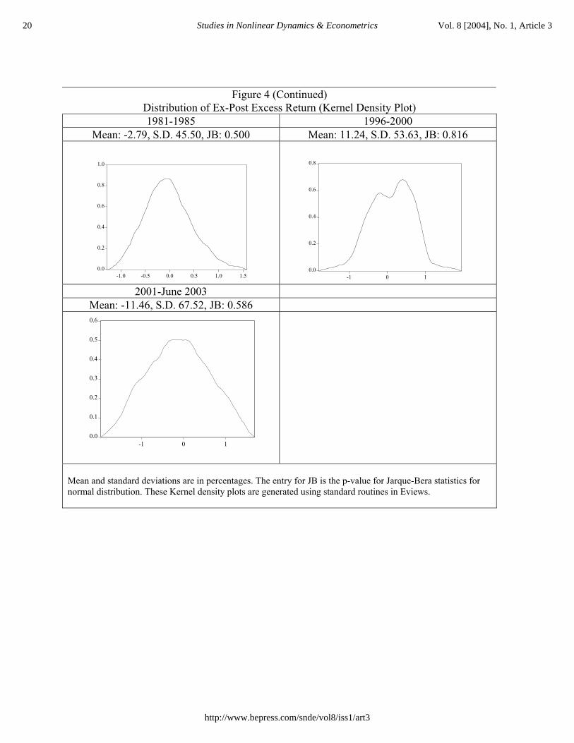
Figure 4 (Continued) Distribution of Ex-Post Excess Return (Kernel Density Plot) 1981-1985 1996-2000

Mean: -2.79, S.D. 45.50, JB: 0.500 Mean: 11.24, S.D. 53.63, JB: 0.816

2001-June 2003 Mean: -11.46, S.D. 67.52, JB: 0.586

Mean and standard deviations are in percentages. The entry for JB is the p-value for Jarque-Bera statistics for normal distribution. These Kernel density plots are generated using standard routines in Eviews.

0.0

0.2

0.4

0.6

0.8

1.0

-1.0 -0.5 0.0 0.5 1.0 1.50.0

0.2

0.4

0.6

0.8

-1 0 1

0.0

0.1

0.2

0.3

0.4

0.5

0.6

-1 0 1



Appendix The index option futures price is assumed to be a function ( , )C F t of the futures price and time. Application of Ito’s lemma implies for C the dynamics (under the historical measure P ),

c cdC dt dZC

µ σ= + , (33)

where

22

2

1 ,2c F F

C C CCt F F

µ µ σ∂ ∂ ∂= + +∂ ∂ ∂

(34)

cF CC F

σ σ∂=∂

, (35)

and ,F Fµ σ are defined in equation (4). We thus have (expressed conveniently in return form) the dynamics (under P ) for ,S F and C . We can use these to obtain the dynamics of the traditional Black-Scholes hedging portfolio, consisting of positions in the three assets. The condition that the hedging portfolio be rendered riskless by appropriate choice of position in each asset can be expressed as the condition that the expected excess return of each asset, risk adjusted by its volatility, be equal to each other. Furthermore the common factor that they all equal is the market price of risk ( λ ) of the source of uncertainty (here the Wiener process Z ) driving the market for the index. Taking into account the continuous dividend yield q on the index and r on the futures, we have ( ) ( )F c

F c

q r r r rµ µ µ λσ σ σ

+ − + − −= = = . (36)

In passing we note that the second equality in (36), after substitution of the expressions for Fµ ,

Fσ , cµ and cσ yields the familiar partial differential equation for C whose solution is given by equation (9). Furthermore we can obtain from (36) that the absence of arbitrage opportunities implies

( ) ,r qµ λσ= − + (37)

,F Fµ λσ= (38)

c crµ λσ= + . (39)



Substituting these into the stochastic differential equations (1), (3) and (33) we can express the arbitrage free dynamics of each asset as

( )( ) ,dS r q Sdt SdZλσ σ= − + +

,F FdF Fdt FdZλσ σ= +

( ) .c cdC r Cdt CdZλσ σ= + +

If we define the new process ( )Z t according to equation (6) then the arbitrage free dynamics assume the form given in (5a, 5b, 5c). We stress that Z is not a Wiener process under the historical measure P , but is under the risk-neutral measure P (after the invoking of Girsanov’s theorem).



References Ait-Sahalia Y., and Lo, A.W. (1998), “Nonparametric Estimation of State-Price Densities Implicit in Financial Asset Prices ”, Journal of Finance, 53(2), 499-549. Babbs, S. H. and Nowman, K. B. (1999), “Kalman Filtering of Generalized Vasicek Term Structure Models ”, Journal of Financial and Quantitative Analysis, Vol. 34, No. 1, March 1999, 115-130. Bekaert, G. and Harvey, C.R. (1995), “Time-Varying World Market Integration”, The Journal of Finance, Vol. L, No. 2, 403-444. Black, F. (1976), “The Pricing of Commodity Contracts”, Journal of Financial Economics, 3, 167-179. Bollerslev, T., Engle, R.F. and Wooldridge, J.M. (1988), “A Capital Asset Pricing Model With Time Covariances”, Journal of Political Economy, 96, 116-131. Bos, T. and Newbold, P. (1984), “An Empirical Investigation of the Possibility of Stochastic Systematic Risk in the Market Model”, Journal of Business, 57, 35-41. Chan, K.C., Karolyi, G.A. and Stulz, R.M. (1992), “Global Financial Markets and the Risk Premium on U.S. Equity”, Journal of Financial Economics, 32, 137-167. Evans, M. D. (1994), “Expected Returns, Time Varying Risk, and Risk Premium”, The Journal of Finance, XLIX, No. 2, 655-679. Fama, E.F. and French, K.R. (2002), “The Equity Premium”, The Journal of Finance, LVII, No.2, 637-659. Ferson, W.E., and Harvey, C. (1991), “The Variation of Economic Risk Premiums”, Journal of Political Economy, 99, 385-415. Hamilton, J.D. (1989), “A New Approach to the Economic Analysis of Non-stationary Time Series Models”, Journal of Econometrics, 70, 127-157. Harvey, A.C. (1989), Forecasting Structural Time Series Models and the Kalman Filter, Cambridge University Press. Jazwinski, A. H. (1970), Stochastic Processes and Filtering Theory, Academic Press, New York, London. Jochum, C. (1999), “Volatility Spillovers and the Price of Risk: Evidence from the Swiss Stock Market”, Empirical Economics, 24, 303-322. Liptser. R. S. and Shiryaev, A. N. (2000), Statistics of Random Processes II, Springer Verlag.



Lo, A. W. (1988), “Maximum Likelihood Estimation of Generalised Ito Processes with Discretely Sampled Data”, Econometric Theory, 4, 231-247. Mayfield, E.S. (2000), “Estimating the Market Risk Premium”, working paper 00-037, Graduate School of Business Administration, Harvard University. Merton, R.C. (1980), “On Estimating the Expected Return on the Market: An Exploratory Investigation”, Journal of Financial Economics, 8, 323-361. McNulty, J.J., Yeh T.D., Schulze, W.S. and Lubatkin M.H. (2002), “What’s Your Real Cost of Capital”, Harvard Business Review, 80(10), 114-121. Wells, C. (1996), The Kalman Filter in Finance, Kluwer Academic Publishers, Boston.



studies in nonlinear dynamics & econometrics volume 8, issue 1 2004 article 3 inferring the...

Documents