structure-conduct-performance - wordpress.com€¦ · · 2016-09-13structure-conduct-performance...

TWO

Structure-Conduct-Performance

Edward S. Mason's (1939,1949) structure-conduct-performance (SCP) approach I~ revolutionized the study of industrial organization by introducing the use ofinfer~

ences from microeconomic analysis. l In the SCP paradigm,2 an industry's perfor~ mance - the success ofan industry in producing benefits for consumers depends~ on the conduct- behavior - ofsellers and buyers, which depends on the structure oftv the market. The structure, in turn, depends on basic conditions such as technology

\' and demand for a product. Typically, research~rs summarize the structure by the number of firms or some other measure of the distribution of firms, such as the relative market shares of the largest firms.

Because the nature of these connections is usually not explained in detail, many economists criticize the SCP approach for beirig descriptive rather than analytic. George J. Stigler (1968) and others urged economists to use price-theory models based on explicit, maximizing behavior by firms and governments rather than the SCP method. Others suggested replacing the SCP paradigm with analyses that emphasized monopolistic competition (Chamberlin 1933, Hotelling 1929), game theory (von Neumann and Morgenstern 1944), or transaction costs (Williamson 1975). Indeed, the rest ofthis book concerns modern empirical alternatives to the SCPo approach.

Mason and his colleagues at Harvard initially conducted case studies ofindividual industries (e.g., Wallace 1937). The first empirical applications of the SCP theory were by Mason's colleagues and students, such as Joe S. Bain (1951, 1956). In contrast to the case studies, these studies made comparisons across industries.

A typical SCP study has two main stages. First, one obtains a measure ofperformance - through direct measurement rather than through estimation - and several measures of industry structure for many industries. Second, the economist uses

1 The following discussion ofstructure--conduct-performance studies draws heavily on Carlton and Perloff (2005), Chapter 8. We are very grateful to Dennis Carlton for his permission to use this material.

2 In all books on industrial organization, SCP is the only acceptable modifier for "paradigm."

13

14 15 Estimating Market Power and Strategies

the cross-industry observations to regress the performance measure on the various structure measures to explain the difference in market performance across industries. We first discuss the measurement ofperformance and structure variables and

then examine the evidence relating performance to structure.

MEASURES OF MARKET PERFORMANCE

Measures of market performance provide an answer to our first key question as to whether market power is exercised in an industry. Measures that directly or indirectly reflect profit or the relationship of price to costs are commonly used to gauge how close an industry's performance is to a competitive benchmark:

• The rate ofreturn is the profit per dollar of investment. • The price-cost margin reflects the difference between price and marginal cost, _

although, in practice, SCP researchers often use some average cost in place of maq;;inal cost. A few studies use just the price based on the assumption that

marginal cost is equal across industries or time. • Tobin's q is the ratio of the market value of a firm to its value based upon the

replacement cost of its assets.

RATE OF RETURN

Determining whether a firm or industry's rate of return differs from the competitive level is difficult. We start by discussing the conceptual approach and then point

out the pitfalls. A firm's profit is revenue less labor, material, and capital costs,

n: = R -labor costs - material costs - (r + 8) Pk K ,

where R is revenue, r is the earned rate of return, 8 is the depreciation rate, Pk is the price of capital, [r + 8]Pk is the rental rate of capital, and K is the quantity

of capital. The competitive earned rate of return is r such that economic profit is

zero:

R labor costs - material costs - 8Pk K (2.1)r

Pk K

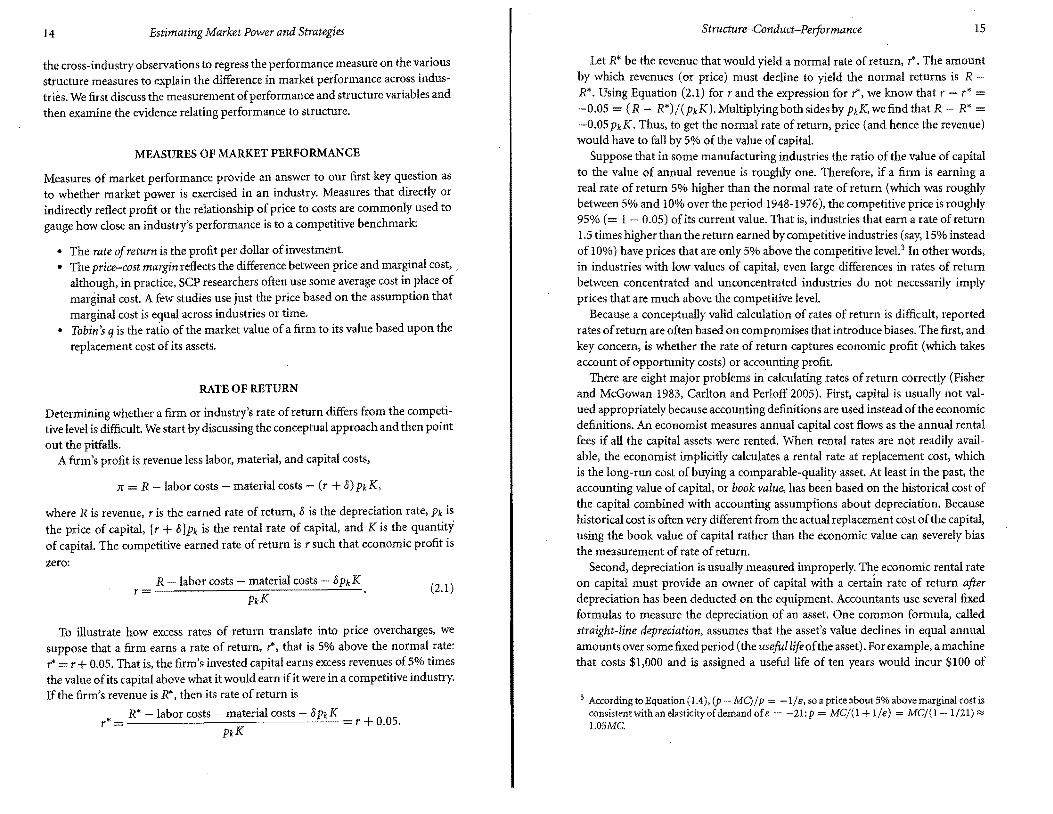
To illustrate how excess rates of return translate into price overcharges, we suppose that a firm earns a rate of return, r", that is 5% above the normal rate: r" r + 0.05. That is, the firm's invested capital earns excess revenues of5% times the value of its capital above what it would earn if it were in a competitive industry.

If the firm's revenue is R*, then its rate of return is

" R" -labor costs - material costs - 8PkK r = r + 0.05.

pkK


Let R* be the revenue that would yield a normal rate of return, r". The amount by which revenues (or price) must decline to yield the normal returns is R R". Using Equation (2.1) for r and the expression for r", we know that r - r* = -0.05 = (R - R*)/(PkK). Multiplying both sides by PkK, we find that R R* = -0.05 PkK. Thus, to get the normal rate of return, price (and hence the revenue) would have to fall by 5% of the value of capital.

Suppose that in some manufacturing industries the ratio of the value of capital to the value of annual revenue is roughly one. Therefore, if a firm is earning a real rate of return 5% higher than the normal rate of return (which was roughly between SOlo and 10% over the period 1948~1976), the competitive price is roughly 95% (= 1 - 0.05) of its current value. That is, industries that earn a rate of return 1.5 times higher than the return earned by competitive industries (say, 15% instead of 10%) have prices that are only 5% above the competitive level. 3 In other words, in industries with low values of capital, even large differences in rates of return between concentrated and unconcentrated industries do not necessarily imply prices that are much above the competitive level.

Because a conceptually valid calculation of rates of return is difficult, reported rates ofreturn are often based on compromises that introduce biases. The first, and key concern, is whether the rate of return captures economic profit (which takes account ofopportunity costs) or accounting profit.

There are eight major problems in calculating rates of return correctly (Fisher and McGowan 1983, Carlton and Perloff 2005). First, capital is usually not valued appropriately because accounting definitions are used instead ofthe economic definitions. An economist measures annual capital cost flows as the annual rental fees if all the capital assets were rented. When rental rates are not readily available, the economist implicitly calculates a rental rate at replacement cost, which is the long-run cost of buying a comparable-quality asset. At least in the past, the accounting value of capital, or book value, has beeIi based on the historical cost of the capital combined with accounting assumptions about depreciation. Because historical cost is often very different from the actual replacement cost ofthe capital, using the book value of capital rather than the economic value can severely bias the measurement of rate of return.

Second, depreciation is usually measured improperly. Threconomic rental rate on capital must provide an owner of capital with a certain rate of return after depreciation has been deducted on the equipment. Accountants use several fixed formulas to measure the depreciation of an asset. One common formula, called straight-line depreciation, assumes that the asset's value declines in equal annual amounts over some fixed period (the useful life ofthe asset). For example, a machine that costs $1,000 and is assigned a useful life of ten years would incur $100 of

3 According to Equation (1.4), (p- MC)/p = -lie, soa price about 50/0 above marginal cost is consistent with an elasticityofdemandofe = -21:p = MC/O + lie) = MC/O-l/21) "" L05MG.


depreciation annually for its first ten years oflife. If it lasts more than ten years, it incurs no additional depreciation ..The fixed formula's predictions of the amount of depreciation may be unrelated to the asset's decline in economic value, which is the measure of its economic depreciation. As a result, the estimate of the rate of return may be biased.

Third, valuing problems arise for advertising and research and development (R&D) because, as with capital, they have lasting impacts. The moneya firm spends on advertising this year maygenerate benefits next year, just as a plant built this year provides a benefit next year. Ifconsumers forget an advertisement's message slowly over time, the advertisement's effect on demand may last for several years. Ifa firm expensed (initially deducted its entire cost of) annual advertising expenditures and then made no deductions in subsequent years, its earned rate of return would be misleadingly low in the initial year and too high in later years. A better approach is to base the advertising expenses on the interest rate and the annual decline in the economic value of the advertising as the annual cost. Unfortunately, it is difficult to determine the correct rates of depreciation to use for advertising expenses.

Fourth, rates of return may not be properly adjusted for risk. To determine whether a firm is earning an excess rate ofreturn, the proper comparison is between the rate of return actually earned and the competitive risk-adjusted rate of return, which is the rate of return earned by competitive firms engaged in projects with the same level of risk as that of the firm under analysis. Investors dislike risk and must be compensated for bearing it: the greater the risk, the higher the expected rate of return. For example, suppose a firm's research to discover new products is successful one time in five. If the firm's expected profit is zero, then the profit on the successful product must be high enough to offset the losses on the four failures. It is misleading to conclude that there are excessively high profits based on an examination of the profit of the one successful product.

Fifth, a related point concerning uncertainty is that some rates of return do not take debt into account properly. Researchers often use the rate ofreturn to the stockholders as a measure ofthe firm's profitability. Ifa firm issues debt in addition to equity, both debt holders and equity holders (stockholders) have claims on the firm's income. Because the assets of the firm are paid for by both debt holders and stockholders, the rate of return on the firm's assets equals a weighted average of the rate of return to the debt holders and the stockholders. The rate of return to debt holders is typically lower than the rate of return to stockholders, because debt is less risky than stock and debt holders get paid before stockholders when a firm is in financial distress. The return to stockholders increases with debt because the income received by stockholders in a highly leveraged firm (one with a high ratio of debt to equity) is risky, so stockholders in such firms demand high rates of return.4

4 Suppose, first, that a firm has no debt and finances an investment with $1,000 raised through sale of stock. Next year, the investment returns the $1,000 plus either $80 or $200 with equal probability, so that the stockholders' rate of return is either 8% or 20% for an average return of


Therefore, it is improper to compare the rates of return to stockholders in two firms in order to measure differences in the degree ofcompetition if the two firms have very different ratios of debt to equity. The debt-equity ratio has nothing to do with whether the firm is earning excess rates of return on its assets. Differences among firms in their rates of return to stockholders could reflect differences in competition facing firms or differences in .their debt-equity ratios. However, even though the rate of return calculated by dividing net income by assets differs from the rate ofreturn from dividing income to stockholders by the value ofstockholder's equity, they tend to be highly correlated (Liebowitz 1982).

Sixth, proper adjustments must be made for infl<).tion. The earned rate of return can be calculated as either a malrate ofreturn (a rate ofreturn adjusted to eliminate the effects ofinflation) or as a nominal rate (which ~ncludes the effects ofinflation). One should be careful to compare rates that are all real or all nominal.

Ifone uses a real rate, income in the numerator of the rate of return should not include the price appreciation on assets from inflation - it should only include the gain in the value of assets beyond that due to general price inflation. For example, ifcapital is initially worth $100, annual income before depreciation is $20, and the annual depredation rate is 100/0 (so depreciation is $10), then the earned rate of return is 10% (20 - 10)/100]. If inflation was 20% during the year, the value of the capital at the end of the year is $90 $100 - depreciation) times 1.2 (to adjust for inflation), or $108. The firm has incurred a gain of $18 on its capital, but it is illusory; it does not represent an increase in purchasing power because all prices have risen as a result of the inflation.

Seventh, monopoly profit may be inappropriately included in the calculated rate of return by using book value in the calculation. Book value sometimes includes capitalized (the present value of future) monopoly profits. Suppose the monopoly earns excess annual economic profits of $100 above the competitive rate of return and the annual interest rate is 10%. The owner of the monopoly sells the firm (and its future stream ofmonopoly profits) for $1,000 more than the replacement cost of its assets. The owner willingly sells the firm because that extra $1,000 will earn $100, or 10%, a year in a bank. The new owner only makes a competitive rate of return because the monopoly profits per year are exactly offset by the foregone interest payments·from the extra $1,000. The extra $1,000 paid for the monopoly is the capitalized value of the monopoly profits, not the replacement

14%. Suppose, instead, that the firm raises the $1 ,000 for the investment by issuing debt of$500 that pays 10% interest and selling stock worth $500. The debt holders must receive payment of interest before the stockholders receive any income. Therefore, whether the firm earns $80 or $200, the debt holders receive $500 plus $50 of interest. The stockholders receive $500 plus either $30 or $150, so that the total amount paid to both debt holders and stockholders is $1,000 plus either $80 or $200. The stockholders therefore earn either 6% (= 30/500) or 30% (= 150/500), for an average return of 18%, whereas the debt holders earn 10%. The stockholders now earn a higher average rate of return and face a wider range of outcomes, even though the income potential ofthe firm is unchanged.


cost to society of replacing the monopoly's capital. Thus, if the reported value of capital inappropriately, includes capitalized monopoly profits, the calculated rate of return is misleadingly low if one wants to determine whether an industry is restricting output and is thereby earning an above normal rate of return.

Eighth, pre-tax rates of return may have been calculated instead ofthe appropriate afterctax rates of return. Corporations pay taxes to the government, and what is left is of interest to individual investors. That is, after-tax rates of return govern entry and exit decisions. Competition among investors causes after-tax rates of return to be equated on different assets. If assets are taxed at different rates, the before-tax rate of return could vary widely even if all markets are competitive. For that reason, we should use after-tax rates of return and after-tax measures of profit, especially when comparisons are made across industries that are subject to

different tax rates.

Price-Cost Margins

In order to avoid the problems associated with calculating rates of return, many economists prefer a different measure of performance, the Lerner index or pricecost margin, L == (p - MC)I p, which is the difference between price, p, and marginal cost, Me, as a fraction of the price. That is, the Lerner index is the percentage markup of price over marginal cost. Because the correlation between accounting rates of return and the price-cost margin can be relatively low (Liebowitz 1982), it makes a difference which of these two performance measures is used.

A competitive firm sets p= MC because its residual demand price elasticity is negative infinity (it faces a horizontal demand curve). As a consequence, L= O.

Unfortunately, because a marginal cost measure is rarely available, many SCP researchers usethe price-average variable cost (AVC) margin instead ofthe appropriate price-marginal cost margin. Their approximation to the price-average variable cost margins is typically calculated as revenue minus payroll minus material cost divided by revenue. (Some researchers commit an even more serious error by using average total cost instead of average variable cost.)

Substituting average variable cost for marginal cost may cause a serious bias (see

Fisher 1987). Suppose that marginal cost is constant and is given as

MC=AVC+(r+ (2.2) q

where r is the competitive rate of return, 8 is the depreciation rate, and AVC is the (constant) average variable cost of the labor and materials needed to produce one unit of output, q. Equation (2.2) describes a technology that requires K Iq units of capital (at a cost of PK per unit of capital) to produce one unit of output.


To show the bias from using AVCin place of MC, we substitute MCfrom Equa

tion (2.2) into Equation (104), (p- Mc)lp = -1/8 (where we suppress the isubscript), to obtain:

P AVC _ ~ + (r + (2.3)p 8

Thus, (p - AVC)lpdiffers from the price-cost margin, (p - MC)lp = -lie, by the lastterm in Equation (2.3), (r+ 8)PKKI(pq), which is the rental value ofcapital divided bv the value ofoutput.

Tobin's q

Tobin's q is less commonly used as a measure ofperformance than either a rate of return or a price-costmargin. Tobin's qis the ratio ofthe market value ofa firm (as measured by the market value ofits outstanding stock and debt) to the replacement cost of the firm's assets (Tobin 1969). If a firm is worth more than what it would cost to rebuild it, then it is earning an excess profit: a profit that is greater than the level necessary to keep the firm in the industry.

By using Tobin's q, researchers avoid the difficult problems assod;lted with estimating rates ofreturn or marginal costs. On the other hand, for q to be meaningful, one needs accurate measures of both the market value and replacement cost of a firm's assets.

It is usually possible to get an accurate estimate for the market value of a firm's assets by summing the values ofthe securities that a firm has issued, such as stocks and bonds. It is much more difficult to obtain an estimate ofthe replacement costs of its assets unless markets for used equipment exist. Moreover, expenditures on advertising and R&D create intangible assets that may be hard to value. Typically, researchers who constructTobin's q ignore the replacement costs ofthese intangible assets in their calculations. For that reason, qtypicaUy exceeds 1. Accordingly, it can be misleading to use q as a measure ofmarket power without further adjustment.

It is pos~ible to determine the degree of monopoly overcharge if Tobin's q is measured accurately. To do so, one must calculate how much earnings (exduding the return to capital) would have to fall for qto equal one. For example, let em be the constant annual earnings ofa monopolyand e, be the constant annual earnings ofa firm under competition. The ratio ofthe market value ofassets to the replacement cost ofassets, q, equals the ratio of em to e,. For example, if q equals two, earnings must fall by one-halfbefore the firm is charging a competitive price.

MEASURES OF MARKET STRUCTURE

To examine how performance varies with structure, we also need measures of market structure. A variety of measures are used; all ofwhich are thought to have


some relation to the degree of competitiveness in an industry. We now describe some of the common measures of market structure.

Firm Size Distribution

Presumably the most important structural issue is the number and relative size of firms. We would expect firrns to exercise more market power if there is only one or a few firms or ifa small number of firms are very large relative to the remaining firms (such as a dominant firm-competitive fringe structure).

In most SCP studies, a measure of industry concentration is used in lieu of a full description ofthe size distribution offirms. Industry concentration is typically measured as a function ofthe market shares ofsome or all ofthe firms in a market.

Concentration Measures. By far the most common variable used to measure the market structure ofan industry is the four-firm concentration ratio (C4), which is the share of industry sales accounted for by the four largest firms. It is, of course, arbitrary to focus attention on the top four firms in defining concentration ratios. Other concentration measures are used as well. For example, the U.S. government also has published eight-firm (C8), twenty-firm (C20), and fifty-firm (C50) concentration ratios.

Alternatively, one could use a function ofall the individual firms' market shares to measure concentration. The most commonly used function is the HerfindahlHirschman Index (HHn, which equals the sum of the squared market shares (expressed as a percentage) ofeach firm in the industry. For example, ifan industry has three firms with market shares of 50%, 30%, and 20%, the HHI equals 3,800 (= [50x50j + [30x30j + [20x20]). More attention has been paid to the HHIsince the early 1980s, when the Department of Justice and Federal Trade Commission started using it to evaluate mergers.

Typically, empirical studies produce similar results for either the HHIor a C4 index. The HHI is the appropriate index ofconcentration to explain prices if firms behave according to the Cournot or other related models (see Cowling and Waterson 1976 and Chapter 1; also see Hendricks and McAfee 2005 for a generalization).

Concentration Statistics. The Bureau ofthe Census irregularly publishes five summary statistics for most four-digit Standard Industrial Code (SIC) manufacturing industries. For decades, the federal government has published summary statistics on industry concentration. However, the most recent publication, U.S. Department of Commerce, Economics and Statistics Administration, Bureau of Census, Concentration Ratios in Manufacturing, 1997 Census of Manufactures (2001), is years out of date. Traditionally, the Bureau of the Census has published four concentration measures - C4, C8, C20, and C50 for most industries. However, for industries with very few firms, some summary statistics are suppressed for reasons of confidentiality. Since 1982, it has also reported the HHI.


Table 2.1. Percent aggregate concentration in the manufacturing sector (measured by value added)

Top firms 1947 1963 1972 1982 1992 1997

50 Largest 17 23 25 24 24 21 100 Largest 23 30 33 33 32 29 200 Largest 30 38 42 43 42 38

Sources: 1982, 1987, 1992, and 1997, U.S. Census Bureau, Census of Manufactures: Concentration Ratios in Manufacturing, Table L

Aside from concentration in individual industries, one can examine concentration in manufacturing in generaL The 1997 Census of Manufactures reports concentration ratios for about 470 manufacturing industries. The C4 was below 40% in more than half ofthe industries, between 41 % and 70% in about one-third ofthe industries, and over 70% in about one-tenth of the industries.

There are now more industries with low C4 ratios and fewer with high C4 ratios than in 1935. In 1935, about 47% ofindustries had a C4 below 40% and about 16% of industries had ratios above 70%. However, since World War II, the distribution of concentration ratios in manufacturing has not changed much. Comparisons based on value, and not on the number of firms in industries, produce similar conclusions.

There has not been a trend toward increasing aggregate concentration in the manufacturing sector based On value added (revenue minus the cost offuel, power, and raw materials) accounted for by the largest firms. Table 2.1 shows that aggregate domestic concentration has increased since 1947, but has remained relatively constant since 1963. Moreover, these domestic concentration statistics overstate concentration because they ignore imports, which have grown in importance.

Most of what we know about concentration ratios concerns manufacturing industries, which comprised only about 17% ofthe gross domestic product (GD P) in 1996. Unfortunately, data on concentration ratios are not readily available for most individual industries outside of manufacturing. It is generally believed that ease ofentry keeps most ofagriculture, services, retailing and wholesale trade, and parts ofmanufacturing and finance, real estate, and insurance relativelyunconcentrated. Moreover, some aggregate measures of concentration in the private sector show that the U.S. economy has become less concentrated overtime in the sense that the.share of employment and assets ofthe largest firms (25, 100, or 200) has declined.

White (2003) provides the first global concentration measures. As trade makes markets international, we need to pay attention to global measures. White reports that in 2001, the largest 500 global companies' employment accounted for 1.6% of the world labor force but 9.9% of OECD employment. He further notes that the large firms' profits were 0.9% ofworld and 1.2% ofOECD GDP.


Problems with Using Concentration Measures. Unfortunately, concentration measures have two serious problems. First, seller concentration measures are affected by many factors. For example, profitability may affect the degree ofconcentration in an industry by affecting entry. One of the key questions we want to answer is whether a more concentrated market structure "causes" higher profits. A test of this hypothesis is only meaningful if structure affects profits but not vice versa. That is, this theory should be tested using exogenous measures of structure, where exogenous means that the structure is determined before profitability and that profitability does not affect structure. Using endogenous measures leads to simul

taneous equation bias. Most commonly used measures of market structure are not exogenous. They

depend on the profitability of the industry. For example, suppose we use the number of firms as a measure of the structure of an industry, arguing that industries with more firms are more competitive. However, entry occurs in extraordinarily profitable industries if there are no barriers to such entry. Although, in the short run, an inherently competitive industry may have a small number of firms, in the long run, many additional firms enter if profits are high.

An exogenous barrier to entry is a better measure ofstructure than the number of firms. For example, ifa government historically prevented entry in a few industries, those industries with the barrier should have higher profits but the higher

do not induce additional entry. Most SCP studies have ignored the problem ofobtaining exogenous measures of

market structure. In particular, the commonly used concentration measures, such as C4, are not exogenous measures of market structure.

The second serious problem is that many concentration measures are biased because of improper market definitions. The relevant economic market for a product includes all products that significantly constrain the price of that product. In order for industry concentration to be a meaningful predictor ofperformance, the industry must comprise a relevant economic market. Otherwise, concentration in

an industry has no implication for pricing. For example, the concentration ratio for an industry whose products compete

closely with those ofanother industry may understate the amountofcompetition. If plastic bottles compete with glass bottles, the concentration ratio in the glass-bottle industry may tell one very little about market power in that industry. The relevant concentration measure should include firms in both industries. Similarly, firms classified in one industry that can modify their equipment and produce products in another industry easily are potential suppliers who influence current pricing but are not reflected in the relevant C4 ratio. If the producers of some Product B could profitably switch production to Product A (Product B is a supply substitute for Product A), then the producers of Product B should also be considered in the

market for Product A. Unfortunately, concentration ratios are published by the government for specific

industries and products, and the definitions used do not necessarily coincide with relevant economic markets. Concentration measures are often based on aggregate

Structure-Conduct-Perjormance

national statistics. If the geographic extent of the market is local because transport costs are very high, national concentration statistics may misleadingly indicate that markets are less concentrated than is true. Some researchers use distance shipped to identify markets in which use ofnational data is misleading: ifthe distance shipped is short, the concentration in the local market may be much different from the national market concentration.

Similarly, concentration measures are often biased because they ignore imports and exports. For example, the 1997 C4 ratio for U.S. automobiles was 80%. This figure indicates a very concentrated industry; however, it ignores the imports of British, Japanese, and German cars, which accounted for more than 23% of total 1997 sales in the United States. The use of improper concentration measures, of course, may bias the estiIAates of the relationship between performance and concentration.

Just as seller concentration can lead to higher prices, buyer concentration can lead to lower prices. When buyers are large and powerful, their concentration can offset the power ofsellers. For that reason, several researchers include buyer concentration as a market structure variable explaining industry performance. The same type of market definition problems can affect this measure. (However, many researchers argue that this measure is more likely to be exogenous than is seller concentration.)

Summary Statistic Biases. Rather than aggregating information about the relative sizes of firms into a single measure, one could examine the effects of the market shares ofthe first, second, third, fourth, and smaller firms on industry performance. For example, one could determine whether increases in the market share of the second firm raise prices by as much as increases in the share of the leading firm. Using this approach, Kwoka (1979) shows that three relatively equal-size firms are much more competitive than two firms.

How well do concentration measures capture information about the size distribution of firms in an industry? Golan, Judge, and Perloff (1 996b ) used generalized maximum entropy (GME) techniques (discussed in the Statistical Appendix) to answer the question of how well one can recover firm shares from summary statistics. To determine whether they could accurately estimate firm shares from summarystatistics, they applied their method to actual data from the Market Share Reporter (Detroit, MI: Gale Research, 1992, 1994) in twenty industries for which there are at least eight firms and the shares reported constitute a substantial majority of the total industry.

They experimented with several approaches. For example, they used the various government concentration measures, C4, C8, C20, and C50, as well as the HHI. Using a Kolmogorov-Smirnov test ofthe hypothesis that the actual and estimated distributions are the same, they could not reject the hypothesis at the 0.05 level for any of their estimates.5

5 The Kolmogorov-Smirnov test is a nonparametric test of whether two distributions are identical.


For the best estimate for each industry, the minimum correlation between the actual and estimated shares is'0.96; the correlation is at least 0.9S for seventeen industries (S5%); and the correlation is at least 0.99 for eleven of our industries (55%). The best estimate ofthe share of the largest firm was never off by more than 2.5 percentage points, and for eleven industries, the estimate was well within one percentage point. Similarly, for sixteen of the industries, the sum of the errors for the first four firms was five percentage points or less.

They also conducted Monte Carlo (simulation) experiments in which they allowed the total number of firms to grow. They found that the accuracy of the firm share estimates for the first ten firms (the ones we care most about) does not change with the total number of firms. When there are many firms, they always estimate the shares of the small firms accurately because those shares are very small

and virtually identical. The availability of particular summary statistics greatly affects our ability to

recover the size distribution ofan industry. To illustrate this point, they repeatedly estimated the shares removing various summary measures from the list ofexplanatory variables one or two at a time. Dropping either C4 or HHIsubstantially reduced their ability to fit the distribution. However, dropping CS and higher concentration measures had relatively little effect on their ability to fit the distribution.

If they dropped all measures save one, they found that the HHI contains more information than C4 or the other concentration measures. Many industrial organization researchers have recently switched from using C4 to the HHI as an explanatory variable in their performance equations, which is consistent with these results concerning the use of a single measure. Of course, one should use all the available summary measures so as to capture as much information about the size distribution

as possible.

Barriers to Entry

Probably the most important structural factor determining industry performance is the ability of firms to enter the industry. In industries with significant long-run entry barriers, prices can remain elevated above competitive levels.6

Commonly used proxies for entry barriers include minimum efficient firm size (the smallest plant that can operate efficiently), advertising intensity, and capital intensity, as well as subjective estimates of the difficulty of entering specific industries. Most empirical studies do not distinguish between long-run barriers to entry and the speed with which entry can occur. The measures they u~e for entry barriers

typically reflect both concepts.

6 There is surprisingly little formal empirical re~earch on entry barriers and the rate of entry. Some relevant articles are Bresnahan and Reiss (1987, 1991) and Dunn, Roberts, and Samuelson (1988).


Fraumeni and Jorgenson (19S0) show that differences in rates of return across industries persist for many years. If there are no long-run barriers to entry or exit, rates of return across industries should converge. Their results indicate that there are long-run barriers, or that the rate of entry and exit is very slow so that convergence in rates of return is slow across industries, or that there are persistent differences across industries in the levels of risk that are reflected in rates of return.

Many commonly used proxies for barriers to entry, such as advertising intensity, are not exogenous. Others, such as subjective measures, have substantial measurement biases.

Unionization

If an industry is highly unionized, the union may be able to capture the industry profits by extracting them through higher wages. Moreover, the higher wages would drive prices up. Therefore, unionization may raise prices to final consumers even though profits to the firms in the industry are not excessive. It is also possible that unions could raise wages and prices and also raise profits to the industry. By making it costly to expand the labor force, unions can prevent industry competition from expanding output and driving profits down. Unionization may not be exogenous if unions are more likely to organize profitable industries.

THE RELATIONSHIP OF STRUCTURE TO PERFORMANCE

There are hundreds, if not thousands, of studies that attempt to relate market structure to each of the three major measures ofmarket performance. This section first discusses the key empirical findings for each of the performance measures based on U.S. data. Then SCP studies based on data from other countries and on data for individual industries are examined. Finally, the section summarizes the major critiques of the results and their interpretation.

Rates of Return and Industry Structure

Joe Bairi's pioneering studies were followed by a voluminous literature investigating the relationship between rates of return and industry structure. Bain (1951) investigated forty-two industries, separating them into two groups: those with a CS ratio in excess of 10% and those with a CS ratio below 70%. The rate of return (calculated roughly as income divided by the book value of stockholders' equity) for the more concentrated industries was I1.S%, compared with 7.5% for less concentrated industries.

Bain (1956) used his subjective judgment to classify industries by the extent of their barriers to entry. He hypothesized that profits would be higher in industries with high concentration and high barriers to entry than in other industries. Bain presented evidence that was consistent with his hypothesis.


Brozen (1971) criticized Bain's findings for two reasons. First, as Bain recognized, the industries that he studied could be in disequilibrium. Brozen showed that the industries Bain identified as highly profitable suffered a subsequent decline in their profits, whereas the industries oflower profitability enjoyed a subsequent increase in profits. In fact, for the forty-two industries of Bain's initial 1951 study, the profit difference of 4.3% that he found between the highly concentrated and less concentrated groups diminished to only 1.1% by the mid-1950s (Brozen 1971). Second, Brozen pointed out that Bain's use, in some ofhis work, of the profit rates of the leading firms, rather than the profit rate of the industry, could have skewed his results.

Using 1950-1960 data, Mann (1966) reproduced many of Bain's original findings. Using the same 70% concentration ratio criterion as Bain used to divide his sample into two groups, Mann found that the rate of return for the more concentrated group was 13.3%, compared with 8% for the less concentrated group.

Mann also investigated the relationship between profit and his own subjective estimates of barriers to entry. He found that industries with very high barriers to entry enjoy higher profits than those with substantial barriers, which in turn earn higher profits than those with moderate to low barriers. He confirmed Bain's predictions and earlier findings that concentrated industries with very high barriers to entry have higher average profit rates than concentrated industries that do not have very high barriers to entry.

There have been many econometric estimates of the relationships among rates of return, concentration, and a variety ofother variables, such as those measuring barriers to entry (see the surveys by Weiss 1974 and Schmalensee 1989). Based on his survey ofmany regression studies, Weiss (1974) concluded that there was a significant relationship among profits, concentration, and barri,ers to entry. Studies based on more recent data tend to find only a weak relationship or no relationship between the structural variables and rates of return. For example, Salinger (1984) found, at best, weak support for the hypothesis that minimum efficient scale in concentrated industries is related to rates of return. Large capital requirements do not constitute a long-run barrier to entry unless other conditions, such as imperfect capital markets or sunk costs, are present. He found no statistical support that his other entry barrier proxy variables - such as advertising intensity - are related to rates of return.

Econometric studies linking profit to market structure often conclude that measured profitability is correlated with the advertising-to-sales ratio and with the ratio of R&D expenditures to sales. These studies also often find that high rates of return and industry growth are related.

Some researchers have studied how the speed of adjustment of capital - and hence profit is related to concentration. Capital-output ratios rise continuously with concentration (see, for example, Collins and Preston 1969). The full explanation for the correlation between capital-output ratios and concentration is not known. One possible explanation for this result is that the plant of minimally


efficient scale is so large relative to industry size that when economies of scale are important, only a few of them can fit into the industry. However, for most industries, minimum efficient scale is a small fraction of total industry demand.

It is possible that the more capital-intensive, concentrated industries use relatively more specialized capital. Ifso, their rates ofadjustment ofthe capital-output ratio should be slower than those ofless concentrated industries because it is u:su-

more difficult to adjust more specialized capital stock. If highly concentrated industries adjust more slowly than unconcentrated industries, that explains why high (or low) profits take longer to fall back to (rise to) the industry average in these industries (Stigler 1963, Connolly and Schwartz 1985, Mueller 1985).

Similarly, ifconcentrated industries take a long time to react to demand changes, then, all else equal, good economic news should raise the value of a company in a concentrated industry more than the value of a company in an unconcentrated industry. Lustgarten and Thomadakis (1980) found that good economic news raises the stock market values ofcompanies in concentrated industries much more than those in unconcentrated industries, and bad economic news lowers their values more.

Price-Cost Margins and Industry Structure

A gigantic literature examines the relationship between price-cost margins and industry structure. The literature varies as to which cost measures are used and which explanatory variables are included.

Price-Average Cost Margins. Following Collins and Preston (1969), many economists examined the relationship across industries between price-average variable cost margins based on Census data and various proxies for industry structure, such as the C4 ratio and the capital-output ratio. A typical regression based on data from 1958 (Domowitz, Hubbard, and Petersen 1986, 1987) is

P AVC PKK. =.16+.10C4+.08--+othervanables, ( 4)

P pq 2. (.01) (.02) (.02)

where P is price,AVC is a measure of average variable cost, C4 is the four-firm concentration ratio, (p - AVC)/ p is the price-average variable cost margin, and pK K / (pq) is the ratio ofthe book value ofcapital to the value ofoutput. The numbers in parentheses below each coefficient are standard errors. The pK K / (pq) term is necessary because price-average variable cost margins 'are t).sed, Equation (2.3).

The sensitivity of price to increases in concentration can be derived from this equation. According to the equation, if the value of capital to annual output, PK K /(pQ), is 40% (the average value across industries), the concentration ratio of the top four firms, C4, is 50%, and if other variables are zero, the predicted


price-average variable cost margin is 0.24 (~.16 + [.lD x .5] + [.08 x .411. or p= 1.3AVC. That is, price is 30% above averag~ variable cost.

Ifthis equation holds over the entire range ofpossible concentration ratio values and the industry's C4 ratio doubles from 50% to lDO%, the price-average variable cost margin rises to 0.29 or p= 1.4AVC. That is, price rises to approximately 1.4 times average variable cost, which is an increase in the price of only about 7%. Thus, even very large increases in concentration may raise price by relatively modest amounts.

For the time period 1958-1981, Domowitz, Hubbard, and Petersen (1986) found that the differential in the price-average variable cost margins between industries of high and low concentrations fell substantially over time. When they estimated a price-average variable cost equation with more recent data, the coefficient associated with the concentration ratio is much lower than its value in 1958. That is, the already small effect of concentration on price in 1958 shrinks in later years. Further, in the later period, a statistical test ofthe hypothesis that the concentration measure does not affect the price-average variable cost margin cannot be rejected. In general, they discovered that the relationship between price-cost margins and concentration is unstable, and, to the extent that any relationship exists, it is weak, especially in recent times.

Instead ofusing industry average variable cost Census data to study the relationship between the price-average variable cost margin and industry structure, other investigators, such as Kwoka and Ravenscraft (1985), use Federal Trade Commission (FTC) data to investigate price-average variable cost margins at the individual firm level. 7 The studies using individual firm data show that the linkbetween higher concentration and higher price-cost margins is ambiguous. Some studies found that the link, if it exists at all, is very weak, whereas others discerned no link at all. They also found that the presence ofa large second or third firm greatly reduces the price-cost margin that can be earned. This discovery indicates that it is a mistake to use only four-firm concentration ratios to measure market structure.

Price-Marginal Cost Margins. One of the main problems in these studies of the relationship between price-cost margins and structure is that they use average cost insteadofmarginal cost. Ifone can directly measure or accurately estimate marginal cost, then one can obtain a good measure ofthe Lerner index and the relationship between the price-cost margin and structure is meaningful. Unfortunately, one can rarely obtain reliable marginal cost measures.

7 The advantage ofusing the firm rather than the industry as the unit of observation is that the researcher can disentangle the effect of industry concentration on a firm's price--cost margin from the effect of the efficiency of that firm alone. For example, one firm's price-cost margin may be high either because the firm is particularly efficient (low cost relative to all other firms) or because all firms in the industry enjoy a high price (lack of competition in the industry). See Benston (1985) for a critique of studies that rely on the Federal Trade Commissiondata.


Table 2.2. Airline price--cost margins and market structure

Share of all Type of market routes

All market types 2.1 100 Dominant firm 3.1 40 Dominant pair 1.2 42

3.3 18 1Wo firms (duopoly) 2.2 19 Dominant firm 2.3 14 No dominant firm 1.5 5 Three firms 1.8 16 Dominant firm 1.9 9 No dominant firm 1.3 7 Four firms 1.8 13 Dominant firm 2.2 6 Dominant pair 1.3 7 No dominant firm or pair" 2.1 ~O

Five or more firms 1.3 35 Dominant firm 3.5 11 Dominant pair 1.4 23 No dominant firm or pair 1.1 0.1

Source: Weiher et al. (2002).

One example where marginal cost measures have been estimated is the airlines industry. Weiher etal. (2002) show that the markup ofprice over long-run marginal

" cost is much greater on routes in which one airline carries most of the passengers than on other routes. Unfortunately, a single firm is the only carrier or the dominant carrier on 58%ofall U.S. domestic routes.

The first column of Table 2.2 identifies the market structure for U.S. air routes. The last column shows the share of routes. A single firm (monopoly) serves 18% of all routes. Duopolies control 19% of the routes, three-firm markets are 16%, four-firm markets are 13%, and five or more firms fly on 35% of the routes.

Although nearly two-thirds ofall routes have three or more carriers, one or two firms dominate virtually all routes. Weiher et al. call a carrier a dominant firm if it has at least 60% ofticket sales byvalue but is not a monopoly. They call two carriers a dominant pairif they collectively have at least 60% ofthe market but neither firm is a dominant firm and three or more firms fly this route. AIl but 0.1% of routes have a monopoly (18%), a dominant firm (40%), or a dominant pair (42%).

The first row of the table shows that the price is slightly more than double (2.1 times) marginal cost on average across all U.S. routes and market structures. average price includes "free" frequent flier tickets and other below-cost tickets.)


The price is 3.3 times marginal cost for monopolies and 3.1 times marginal cost for dominant firms. In contrast, over the sample period, the average price is 1.2 times marginal cost for dominant pairs.

The markup ofprice over marginal cost depends much more on whether there is a dominant firm or dominant pair than on the total number of firms in the market. If there is a dominant pair, whether there are four or five firms, the price is between 1.3 times marginal cost for a four-firm route and 1.4 times marginal cost for a route with five or more firms. If there is a dominant firm, price is 2.3 times marginal cost on duopoly routes, 1.9 timeson three-firm routes, 2.2 times on four-firm routes, and 3.5 times on routes with five or more firms.

Thus, preventing a single firm from dominating a route may substantially lower prices. Even if two firms dominate the market, the markup ofprice over marginal cost is substantially lower than if a single firm dominates.

Other Explanatory Variables. Various studies report significant effects from other explanatory variables. Kwoka and Ravenscraft (1986) learned that industry growth has a significant and positive effect on price-average variable cost margins. Lustgarten (1975) concluded that increased buyer concentration sometimes lowers price--cost margins. Comanor and Wilson (1967) reported that a higher advertising-sales ratio may raise the price-cost margin.

Freeman (1983) showed that unions lower the price--cost margin. Salinger ( 1984) and Ruback and Zimmerman (1984) also found that unionism has a significant negative effect on the profits of highly concentrated industries. Voos and Mishel (1986) reported that, although unions may depress the price--cost margin, the price is not significantly above the price that would prevail in the absence of a union.

International Studies of Performance and Structure

Because international trade is more important in many other countries than in American markets, the bias from ignoring imports and exports may be more substantial in studies based on data from those countries than in those based on u.s. data. Concentration ratios based only on domestic concentration may not be economically meaningful as measures ofmarket power. The relevant competition may well be from firms located outside a given country.

Nonetheless, despite differences across countries in sizes of domestic markets, domestic concentration ratios are correlated across countries (Pryor 1972). That is, an industry that is concentrated in the United States is also likely to be concentrated in the United Kingdom. However, the correlation is not perfect, as illustrated by Sutton (1989) for the U.S. and U.K. frozen food industries.

Regardless ofwhich country's data are used, most studies have difficulty detecting an economically and statistically significant effect ofconcentration on performance (Hart and Morgan 1977, Geroski 1981). However, Encoau and Geroski (1984)


found that the United States, the United Kingdom, and Japan tend to have sloW' rates ofprice adjustment in their most concentrated sectors.s

Performance and SJructure in Individual Industries

Most studies of SCP are based on cross-sectional data rather than data for a particular industry over time (though there are exceptions, like Weiher et al. 2002). There are two serious shortcomings in cross-sectional studies of the relationship between structure and performance across different industries.

First, it is unrealistic to expect the same relationship between structure and performance to hold across all industries. Suppose that one monopolized industry has a high elasticity of demand, and another monopolized industry has a low elasticityofdemand. As Equation (2.2) shows, the price-costmargin in the industry with the high elasticity of demand is lower than the price-cost margin in the industry with the low elasticity of demand. Most cross-sectional studies fail to control for differences in demand elasticities across industries, thereby implicitly assuming that the elasticities are identical across industries.

Second, it is unlikely that the C4 ratios published by the U.S. Census correspond to the concentration ratios for relevant economic markets. Ifconcentration ratios are notdefined for the proper markets, one should not expectto find any correlation between performance and concentration across different markets.

Measurement and Statistical Problems

In summary, there is, at best, weak evidence of a link between concentration and various proxies for barriers to entry and measures ofmarket performance. Are the theories concerning the relationship between performance and structure wrong or are these studies flawed?

Although many SCP studies are well done, others are seriously flawed. These are discussed in the next section. Many ofthe negative findings in these studies may be due to two important problems. First, many ofthese studies suffer from substantial measurement or related statistical problems that are difficult to correct. Second, and more importantly, most of these studies are conceptually flawed. Many of these measurement and statistic problems were discussed earlier. Three additional problems are analyzed here.

First, concentration measures and performance measures are frequently biased due to improper aggregation across products. Because most firms sell more than one product, any estimate ofprofits or price-cost margins for a firm reflects averages across different products. For a firm that makes products in many different industries, aggregate statistics can be misleading. For example, the Census assigns

B The industrial organization ofJapan is discussed in Caves and Uekasa (1976) and Miwa (1996).


firms to industry categories based on the primary products produced and includes their total value ofproduction under that industry category. The Census also tabulates statistics at the product level, based on data from individual plants. Because a plant is less likely than a firm to produce several products, product-level data are preferable because such data are less likely to have an aggregation bias than industry-level data.

Second, as already mentioned, the performance and structural variables tend to suffer from other measurement errors. Some researchers include variables in addition to concentration to control for such measurement problems in an attempt to reduce these biases. For example, because most price-cost margins ignore capital and advertising, some economists include those two variables in their regressions of

variables may not eliminate the bias if they are measured with error or determined by industry profitability (that is, endogenous). For example, researchers frequently mismeasure advertising, and advertising may be more heavily used in highly profitable industries.

Third, many studies inappropriately estimate linear relations between a measure ofperformance and concentration. For example, if increases in concentration have increasingly large effects on performance as the concentration rises up to a critical level and thereafter increases in concentration have relatively little additional effect, the relationship between performance and concentration will resemble an S-shaped curve: first concave and then convex to the horizontal axis. This ...r-"U<'IJ~,U curve can be approximated reasonably by a straight line only if the observed levels ofconcentration lie in some restricted range. Ifconcentration ratios vary from very low levels to very high levels, an estimate based on a presumed linear relationship may lead to incorrect results.

White (1976) and Bradburd and Over (1982) searched for critical levels of concentration below which price is less likely to increase as concentration increases, and threshold levels of concentration above which price is more likely to increase as concentration increases. They were only partially successful in finding such a level: there appears to be some evidence of an increase in price at C4 ratios above

50% to 60%. and Over (1982) present evidence that the effect of concentration on

an industry's performance depends on levels of past concentration. As a concentrated industry becomes less concentrated, price remains higher than it would if the industry had never been highly concentrated.

Conceptual Problems

The measure of performance is viewed as evidence about the existence of market power. Most SCP studies are interested in determining whether there is a relationship between performance (such as market power) and industry structure. However, the conceptual problems inherent in these studies limit their ability to

Structure-Conduct-PerJormance

relationship. The two most common conceptual problems concern performance measures are used and whether the structural vari

abIes are exogenous. Although standard, static economic theories hold that long-run profits vary with

market structure, they say nothing about the relationship ofshort-run profits and market structure. Thus, a SCP study based on short-run performance measures is not a proper test of the theories.

The amount of time needed to reach the long run differs by industry. At any moment, some industries are highly profitable whereas others are not. Over time, some firms exit from the low-profit industries and enter the high-profit industries, which drives rates of return toward a common level. Stigler (1963), Connolly and Schwartz (1985), and Mueller (1985) find that high profits often decline slowly in

concentrated industries. It is only by analyzing the level ofprofits (or other measures ofperformance) and the rate at which they change that the analyst can distinguish between a long-run barrier to entry and the speed with which entry occurs. Most analyses do not make this distinction. This problem may be regarded as one of accurately measuring performance.

However, the various measurement problems with performance may not be as serious as they first appear. Schmalensee (1989) used twelve different accounting measures ofprofitability in a SCP study. Strikingly, although these twelve measures are not highly correlated, many ofhis SCP results held over all measures.

Perhaps the more serious conceptual problem with many SCP studies is that the structural variables are not exogenous. Many researchers, after finding a link between high profits (or excessive rates or return, large price-cost margins, values ofq) and high concentration ratios, infer improperly that high concentration rates are bad because they "cause" high profits.

However, profit and concentration influence each other. An alternative interpretation of a link between profits and concentration is that the largest firms are the most efficient or innovative (Demsetz 1973, Peltzman 1977). Only when a firm is efficient or innovative is it profitable to expand in a market and make the market concentrated. In this interpretation, a successful firm attracts consumers, either through lower prices or better products. A firm's success, as measured by both its profit and its market share, is an indicator of consumer satisfaction, not an indicator of poor industry performance. One implication of this hypothesis is that a firm's success is explained by its own market share and not just by industry concentration, as found by Kwoka and Ravenscraft (1985).

If concentration is not an exogenous measure, then an estimate ofthe relationship between profits and concentration, which assumes that concentration affects profits and not vice versa, leads to what is referred to as a simultaneity bias. However, Weiss (1974) estimated the relationship between performance measures and concentration using statistical techniques designed to eliminate the simultaneity bias problem and found that the different estimation procedures make little difference in the estimated


Although the regression results may not change, their interpretation does. Even a correctly estimated relationship between performance and concentration is uninformative regarding causation. High profits are not caused by concentration, but are caused by long-run barriers to entry. These barriers cause both high profits and high concentration.

Research using the SCP approach continues, though at a reduced rate. Some relatively recent works include Marvel (1978), Lamm (1981), Cotterill (1986),

Schmalensee (1987), Cubbin and Geroski (1987), and Sutton (1991).

A MODERN STRUCTURE-CONDUCT-PERFORMANCE APPROACH

There is one other important modern approach to SCP by Sutton (1991, 1998).

Sutton uses a game-theoretic approach to examine what happens to competition, promotional activities, and R&D as market size grows. He also addresses what happens if sunk costs are endogenous.

The original SCP literature sought to establish a systematic relationship between price and concentration. We have discussed many criticisms of this approach, but perhaps the most significant is that concentration itself is determined by the economic conditions of the industry and hence is not an industry characteristic that can be used to explain pricing or other conduct. The barrage of criticisms caused most research in this area to cease in recent years. However, Sutton has developed an approach that builds on the SCP idea oflooking for systematic patterns ofcompetitive behavior across industries, and, at the same time, addresses the endogenous determination of entry (Sutton 1991, 1998).

Sutton's research examines what happens to competition as the size ofthe market grows. Does the market become less concentrated? Do other dimensions of the product - such as quality, promotional activity, and R&D - change? What are the fundamental economic forces that provide the bases for systematic answers to these questions across different industries? In answering these questions, Sutton analyzes markets in which the product is either homogeneous or heterogeneous and considers the cost of entering the market or altering certain attributes of products.

Theory

Sutton examines two cases depending on whether a firm's cost of entry is an exogenous sunk cost or an endogenous sunk cost. In the former case, each firm must spend some fixed amount, F, to enter the industry. In the latter case, the amount a firm must spend to enter the industry is variable and is chosen by the firm in an effort to affect the desirabilityofits product by influencing certain dimensions ofthe product.


Exogenous Sunk Cost. To illustrate his theory, Sutton examines markets with homogeneous and heterogeneous products. Initially, we consider a market in which the firms produce a homogeneous product and the only variable on which firms can compete is price (not quality). Each firm incurs a sunk fixed cost F and has a constant marginal cost m. At low prices, the industry demand curve is Q = s/p, where Qis industry quantity, s is a measure ofmarket size (total expenditure, which is assumed to be determined independent of price), and Pis price. That is, for low prices and given s, the market elasticity of demand is -1. At some high price Pm, the demand curve is perfectly elastic. Thus, a monopoly would charge a price of Pm in this market.

The final equilibrium and how the equilibrium will change as the market size grows are determined by the form that competition takes. To fix ideas, Sutton considered three types of competition, each "tougher" than the next. The level of competition is lowest in a cartel in which all firms explicitly collude to set the monopoly price Pm and divide up the total cartel or monopoly profit among the n firms. Regardless of the number of firms, n, the price remains at Pm. Thus, profit per firm declines as n grows because the total monopoly profit is divided among more and more firms. The equilibrium n is the one at which that the total cartel profit is driven to zero.9

A more competitive market is a Cournot oligopoly. For any number of firms, n, the equilibrium Cournot price is p(n) = m[l + 1/(n - 1)J.lO Thus, the Cournot price P falls to m as n increases. The output per firm, q, equals (s/m)[(n - 1)/n2], and profit per firm is [p - mJq - F, which equals s/n2

F. Hence, with free entry, n equals .fSTF, at which point profit per firm is zero.

Finally, consider the most competitive equilibrium, Bertrand, where price equals m.for any given n > 1. Here, the only free-entry equilibrium has one firm with positive profit. Were a second firm to enter, it would drive price to marginal cost, so that its profit would be negative (accounting for the fixed cost).

For each model ofcompetition, Figure 2.1 shows how price changes as nincreases. As the figure illustrates, for any given n > 1, price is lower as competition becomes "tougher," with Bertrand being the toughest and cartel being the least tough model of competition.

9 Let the cartel profit be n = [p - mJ Q- nF. The price that maximizes cartel profit is the same price that maximizes [p - mJQ. Define nm , the profit ignoring fixed costs, as the maximum of [p - mJQ. Then, each firm's individual profit is nm/n - F. In equilibrium where n = 0,

. the equilibrium n equals nm/F. 10 Each firm selects its output qi to maximize its profit, which can be written as Pi(~qj)qi

mqi - F, where Pi(~Ilj) is the inverse demand curve. Differentiating this expression with respect to qi yields the first-order condition for each firm's optimal output level given its rival's output levels. Setting qi = q for all i yields the symmetric Cournot equilibrium (assuming that the resulting price is less than Pm).

36 37

Estimating Market Power and Strategies

p

,ol • Cartel

Cournot m \, • • Bertrand

2 4

Number of firms, n

Figure 2.1. Relationship Between Prices and Number of Firms Under Three Market Structures. Sources: Sutton (1991, 1998).

Figure 2.2 relates a measure ofequilibrium industry concentration, 1/n, to market size 5 for each model ofcompetition, where, by equilibrium market concentra

we mean that n at which total profit equals zero (or more accurately, if one additional firm enters, it will earn a negative profit.)

Figure 2.2 reveals two interesting results. First, as expected, concentration falls as market size increases for all but the most competitive game (Bertrand). The intuitionJor this result is that larger markets can accommodate more firms.

The second result is counterintuitive: for any given market size, when equilibrium market concentration is higher, the tougher the competition. Concentration is lowest for the cartel model, even though the cartel model has the highest price. The reason for this result is that tough competition leads to a low price, which discourages entry. This result illustrates that relying on concentration alone to make inferences about price and competitiveness can lead to erroneous conclusions.

The case of exogenous fixed costs with heterogeneous products has much less crisp results than the case ofexogenous fixed costs with a homogeneous product. In a model with heterogeneous products, the concentration in the market depends on the nature of the game, such as how many different products one firm may produce and whether a firm has an advantage if it can choose its products before other firms choose.

Sutton's main result for heterogeneous products is that the "toughness" ofcompetition is, in general, diminished when one moves from a homogeneous to a heterogeneous product and so (analogous to the result that occurs in the case of homogeneous product as competition weakens) the equilibrium concentration tends to fall for any given market size s. However, unlike the case ofa homogeneous product, there are many possible equilibrium outcomes for any market size, 5, and the best that an economist can derive is a lower bound on concentration for any given s. When this lower bound is low, it means that there are very few

Structure-Conduct-Per!ormance

lIn, Concentration I

1 ~ Bertrand

1/2

1/3

Cournot1/4

Cartel

S, Market size

Figure 2.2. Relationship Between Concentration and Market Size Under Three Market Structures. Sources: Sutton (1991, 1998).

empirical predictions one can make about equilibrium concentration because any equilibrium concentration is possible as long as it exceeds the lower bound.

The property that equilibrium concentration (orits lower bound) decreases with market size s depends on the assumption that fixed costs are exogenous and that product quality is given. Given this property, all else equal, concentration should be lower in big countries than in small countries, when market size is determined by the size of country.

Although this result holds for many industries, there are some industries that are highly concentrated in both large and small countries. Sutton explains this mystery using endogenous sunk costs.

Endogenous Sunk Costs. In most markets, firms compete not just on price but also along many other product dimensions such as quality, reliability, R&D, or promotional activity. The key new assumption is that a firm may spend money to improve its product's W, an index of quality, which we will broadly interpret to include information about the product. In this model, the fixed entry cost, F(W), depends on the quality index. For examp Ie, firms increase their advertising expenditures' R&D expenditures, and engineering expenditures to increase Wby raising the quality of the product or by increasing consumers' perception of its Firms can compete for customers by spending money to improve product quality, by lowering price, or by doing both. Here, we say that the firm has endogenous sunk costs because the firm decides how large an investment to make.

Paying to improve quality has two important effects. First, it raises the firm's fixed cost and perhaps its marginal cost ofproduction ifa higher quality good costs more to produce. Second, it attracts customers who were previously buying a lower


quality good. These two effects can combine to reverse completely the results in the previous section in which an increase in market size is associated with a decrease in equilibrium concentration. As market size 5 increases, firms have an incentive to compete by improving the quality W of their product. To raise quality, a firm must incur larger sunk costs, which reduces the incentive for additional firms to enter the industry that otherwise arises from the larger s. As a result, as market size increases, concentration no longer necessarily falls. A given industry in different sized markets can remain highly concentrated, but bigger markets will have higher quality products.

For this reasoning to be valid, several assumptions need to hold. Consumers must value improvements in quality sufficiently so that they switch from lower products to higher quality ones. To establish the condition under which this is so, Sutton uses a model of vertical differentiation. In such a model, every consumer agrees on a ranking of products by quality, W, with all consumers preferring a higher quality product to a lower quality product.

Suppose that a consumer's surplus from a good ofquality Wequals U = $ W where $ is a parameter reflecting the weight that the consumer places on

quality and p(W) is the price of a product with quality W. Because consumers differ in $, even though all consumers prefer more W to less, some consumers place such a low value on extra W that they are willing to pay very little extra money for a high W product, whereas other consumers so enjoy extra quality that they will buy a higher quality good even if the price is relatively high. The optimal W for any consumer will depend on the price function p( W), which reveals how prices rise as W rises, and on the consumer preference, $, for

Sutton proves that as long as p( W) and the marginal cost of producing a quality product do not rise "too mst" as Wincreases, then the equilibrium has three striking properties. First, the firms that produce the highest quality available in the market are the largest firms.

Second, an increase in market size leads to an increase in the quality of the best products in the market, higher quality products being chosen by consumers at higher prices and some lower quality products disappearing from the market.

the equilibrium quality rises as' the market expands. Third, with higher quality and its attendant costs, fewer firms can afford to

remain in the industry and concentration will remain high. Consequently, the property that a market remains concentrated as s increases continues to hold even where there is both horizontal and vertical differentiation as long as there is sufficient substitution between the vertical dimension (quality VV) and the horizontal dimension over which consumers can have different preferences.

For both the endogenous and exogenous sunk cost cases, the key empirical predictions about concentration and market size depend on the validity of certain assumptions. The most important one is that the form of the game - Bertrand, Coumot, or cartel- remains unchanged as market size increases. In a given market, this assumption mayor may not be plausible. Moreover, neither Sutton nor anyone


else has made significant progress on describing the industry economic characteristics that predict the form of the game that describes the competitive process. Therefore, analogous to the criticism of the earlier literature that concentration need not be exogenous, here we have the criticism that the form ofthe competitive game need not be exogenous.

Empirical Research

Sutton has produced two voluminous books (1991, 1998) of studies using data from France, Germany, Italy, Japan, the United Kingdom, and the United States to test his theories, especially those concerning the endogeneity ofadvertising and technology. Sutton's empirical work helps explain why concentration is similar across different size countries for some industries but not others.

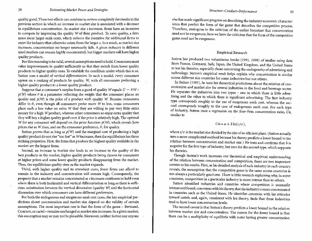
In Sutton (1991), he tests his theoretical predictions about the relation of concentration and market size for several industries in the food and beverage sector. He separates the industries into two types - one in which there is little advertising and the other in which there is significant advertising. The first industry type corresponds ,roughly to the use of exogenous sunk cost, whereas the second corresponds roughly to the case of endogenous sunk cost. For each type of industry, Sutton runs a regression on the four-firm concentration ratio, similar to

C4=a+ b

where sla is the market size divided by the size ofan efficient plant. (Sutton actually uses a more complicated method because his theory predicts a lower bound to the relation between concentration and market size.) He tests and confirms that b is negative for the first type ofindustry, but zero for the second type, which supports his theories.

Though Sutton's work increases our theoretical and empirical understanding of the relation between concentration and competition, there are two important caveats to his results. First, as his detailed analysis ofeach industry in each country reveals, the assumption that the competitive game is the same across countries is not always a particularly good one. There is little research explaining why, in sOllle countries, competition in a particular industry is more intense than in others.

Sutton identified industries and countries where competition is unusually intense andfound, consistent with his theory, that the industry is more concentrated in countries such as the United States. He identifies countries with lax attitudes toward cartels and, again, consistent with his theory, finds that those industries tend to have lower concentration levels.

The second caveat is that Sutton's theory predicts a lower bound to the relation between market size and concentration. The reason for the lower bound is that there can be a multiplicity of eqmlibria with some having greater concentration

40 41

Estimating Market Power and Strategies

levels than the lower bound. The theory, therefore, is unable to help us much in predicting concentration in a particular country when the lower bound is low.

Although Sutton explains that this theory of lower bounds is the most one can say under general conditions, it leaves the analyst in the uncomfortable position of having a theoretical structure that may not narrow the possible equilibria very much. Sutton's detailed history of each industry shows that many idiosyncratic factors often are critical in explaining an industry's evolution. Thus, his work provides a sobering lesson because it reveals the limits oftheoryto explain industrial structures.

SUMMARY

SCP studies assume that the degree ofmarket power our first question can be answered using commonly available statistics as proxies for market power. These studies focus on the causes of market power our second question. Traditionally, SCP studies use cross-sectional industry data to explain variations in market power across industries as a function of concentration and other factors.

In the following chapters, we turn to other, modern approaches to examining our key questions. These studies differ substantially from traditional SCP studies. Most recent studies concentrate on estimating market power rather than using published proxies. Because these studies usually examine only a single firm or industry over time, they cannot explain differences across industries.

PROBLEMS

Note: Answers to problems are available at the back of the book.

2.1 Suppose that the firms in a market are engaged in a Cournot game' and that Firm 1's Lerner's index is Li = (p mj)lp = 5;/e, where Sj is Firm i's quantity share of the market. Cowling and Waterson (1976) observed that the weighted average price--cost margin for the industry is Li(P - mi)1 P = - Li slie -HHlle [see Equation (1.6) in Chapter I], where HHIis the Herfindahl-Hirschman Index. Suppose Equation (2.2) holds so that mi=AVCi + (r + 8)PKK;/q;. Many empirical researchers have used (p - AVC;)Ip instead of (p mj)Ip in their empirical studies. Derive an expression sirnilarto Cowling and Waterson's equation relating (p AVq)lp to the HHI to show the effect of using this alternative measure.

2.2 Traditionally, SCP empirical studies estimated an equation relating a profit measure to a concentration measure using ordinary least squares. One of the major criticisms is that concentration is an endogenous variable. You are asked to show the relationship between a measure ofprofitability, piMC, and the C4 concentration measure. Consider a monopolistically competitive industry in which firms produce a homogeneous product, demand is linear (p a - bQ,

Structure-Conduct-Per!ormance

where p is price and Q is total output), firms have identical cost functions (constant marginal cost m plus a fixed cost F), and they play Coumot. Firms enter until the number of firms, n, is such that the marginal firm makes a zero profit. Solve for the eqUilibrium number of firms, quantities, and price. (For simplicity, allow n to be a non-integer.) Show how the quantity per firm, price, number of firms, piMC, and C4 change as F increases.

2.3 Given exogenous sunk costs, Sutton (1991, 1998) shows that, for any given market size, equilibrium market concentration is higher the more competitive is the market (the Bertrand equilibrium is more competitive than the Coumot equilibrium, which is more competitive than the cartel outcome), Why? What implications does this result have for traditional SCP empirical studies?

structure-conduct-performance - wordpress.com€¦ · · 2016-09-13structure-conduct-performance...

Documents