structural design parameters of current wsdot mixtures · jacob meader. june 2013 donald janssen....
TRANSCRIPT

June 2013Jacob MeaderDonald JanssenMarc Eberhard
WA-RD 802.1
Office of Research & Library Services
WSDOT Research Report
Structural Design Parametersof Current WSDOT Mixtures


Final Research Report Agreement T4118, Task 79
Structural Design
STRUCTURAL DESIGN PARAMETERS
OF CURRENT WSDOT MIXTURES
by
Jacob D. Meader Graduate Research Assistant
Donald J. Janssen Associate Professor
Marc O. Eberhard Professor
Washington State Transportation Center (TRAC) University of Washington, Box 354802
University District Building 1107 NE 45th Street, Suite 535
Seattle, Washington 98105-4631
Washington State Department of Transportation Technical Monitor
Ron Lewis Bridge Project Engineer, Tumwater, WA 98501
Prepared for
The State of Washington Department of Transportation
Lynn Peterson
June 2013

TECHNICAL REPORT STANDARD TITLE PAGE
1. REPORT NO. 2. GOVERNMENT ACCESSION NO. 3. RECIPIENT'S CATALOG NO.
WA-RD 802.1 4. TITLE AND SUBTITLE 5. REPORT DATE
STRUCTURAL DESIGN PARAMETERS OF CURRENT WSDOT MIXTURES
June 2013 6. PERFORMING ORGANIZATION CODE
7. AUTHOR(S) 8. PERFORMING ORGANIZATION REPORT NO.
Jacob Meader, Donald J. Janssen, Marc O. Eberhard 9. PERFORMING ORGANIZATION NAME AND ADDRESS 10. WORK UNIT NO.
Washington State Transportation Center (TRAC) University of Washington, Box 354802 University District Building; 1107 NE 45th Street, Suite 535 Seattle, Washington 98105-4631
11. CONTRACT OR GRANT NO.
Agreement T4881, Task 79
12. SPONSORING AGENCY NAME AND ADDRESS 13. TYPE OF REPORT AND PERIOD COVERED
Research Office Washington State Department of Transportation Transportation Building, MS 47372 Olympia, Washington 98504-7372
Project Manager: Kim Willoughby, 360.705.7978
Final Research Report 14. SPONSORING AGENCY CODE
15. SUPPLEMENTARY NOTES
This study was conducted in cooperation with the U.S. Department of Transportation, Federal Highway Administration. 16. ABSTRACT:
The AASHTO LRFD, as well as other design manuals, has specifications that estimate the structural performance of a concrete mixture with regard to compressive strength, tensile strength, and deformation-related properties such as the modulus of elasticity, drying shrinkage, and creep. The Washington State Department of Transportation (WSDOT) is evaluating the performance properties of approved concrete mixtures, and verifying the measured properties and comparing them to those expected from AASHTO specifications. Factors influencing the structural behavior of concrete mixtures include the coarse aggregate source and size, paste content, water-to-cementitious ratio, and age characteristics. These factors are not integrated within AASHTO LRFD models to predict the concrete mixture’s performance. Current specifications relate most of the structural performance properties to the compressive strength, with little regard to the mixture proportions. This research was directed toward assessing the performance of the approved WSDOT concrete mixture and the sensitivity of the properties based on aggregate source and paste content. The objectives of this research were to investigate whether modifications to AASHTO LRFD specifications were required, and if so, to recommend improvements using pertinent mixture proportions.
17. KEY WORDS 18. DISTRIBUTION STATEMENT
Compressive strength, split-tensile strength, flexural strength, elastic modulus, drying shrinkage, creep strain, creep coefficient, and specific creep.
No restrictions. This document is available to the public through the National Technical Information Service, Springfield, VA 22616
19. SECURITY CLASSIF. (of this report) 20. SECURITY CLASSIF. (of this page) 21. NO. OF PAGES 22. PRICE
None None

DISCLAIMER
The contents of this report reflect the views of the authors, who are responsible
for the facts and the accuracy of the data presented herein. The contents do not
necessarily reflect the official views or policies of the Washington State Department of
Transportation or Federal Highway Administration. This report does not constitute a
standard, specification, or regulation.
iii

iv

Table of Contents
Disclaimer .......................................................................................................................... iii Executive Summary ...........................................................................................................xv
Problem Statement ...............................................................................................xv Research Goals .....................................................................................................xv Research Approach ...............................................................................................xv Findings and Recommendations: ....................................................................... xvi
Compressive Strength ................................................................................ xvi Tensile Strength ......................................................................................... xvi Elastic Modulus ........................................................................................ xvii Shrinkage .................................................................................................. xvii Creep ....................................................................................................... xviii
Chapter 1: Problem Statement .............................................................................................1 Chapter 2: Background and Literature Review ...................................................................3
2.1 Compressive Strength .......................................................................................3 2.2 Tensile Strength ................................................................................................4 2.3 Elastic Modulus ................................................................................................4 2.4 Drying Shrinkage .............................................................................................6 2.5 Creep ................................................................................................................7
Chapter 3: Test Program ......................................................................................................9 3.1 WSDOT Projects Sampled ...............................................................................9 3.2 Laboratory Mixtures .......................................................................................10 3.3 Tests Performed ..............................................................................................12 3.4 Specimen Preparation and Testing .................................................................13
3.4.1 Compressive Strength Test Procedure ...............................................13 3.4.2 Tensile Strength Test Procedure .........................................................14 3.4.3 Elastic Modulus Test Procedure .........................................................14 3.4.4 Drying Shrinkage Test Procedure ......................................................15 3.4.5 Creep Test Procedure .........................................................................15
Chapter 4: Compressive Strength ......................................................................................19 4.1 Laboratory Data for DuPont (3/4-in.) Aggregate Source ...............................19
4.1.1 Measured Compressive Strengths ......................................................19 4.1.2 Rate of Strength Gain .........................................................................21
4.2 Laboratory Data for All Aggregate Sources ...................................................24 4.2.1 Summary of Measured Compressive Strengths .................................25 4.2.2 Rate of Strength Gain .........................................................................27
4.3 Data for Field Samples ...................................................................................29 4.3.1 Measured Compressive Strengths ......................................................29 4.3.2 Rate of Strength Gain .........................................................................31 4.3.3 Variability ...........................................................................................33
4.4 Analysis of Compressive Strength Results ....................................................34 Chapter 5: Tensile Strength ...............................................................................................35
5.1 Flexure Tests ..................................................................................................36 5.2 Split-Tension Tests .........................................................................................40 5.3 Relationship between Split-Tension and Flexure Strengths...........................42
v
5.4 Summary of Tensile Strength Results ............................................................43 6.1 Laboratory Data for DuPont (3/4-in.) Aggregate Source ...............................45
6.1.1 Measured Elastic Modulus .................................................................45 6.1.2 Rate of Stiffness Gain .........................................................................48
6.2 Laboratory Data for All Aggregate Sources ...................................................52 6.2.1 Measured Elastic Moduli ....................................................................52 6.2.2 Rate of Stiffness Gain .........................................................................56
6.3 Data for Field Samples ...................................................................................58 6.3.1 Measured Elastic Moduli ....................................................................58 6.3.2 Rate of Stiffness Gain .........................................................................62 6.3.3 Variability ...........................................................................................65 6.3.4 Comparison of Laboratory and Field Data .........................................66
6.4 Analysis of Elastic Modulus Results ..............................................................68 Chapter 7: Drying Shrinkage .............................................................................................69
7.1 Laboratory Data for DuPont (3/4-in.) Aggregate Source ...............................69 7.2 Laboratory Data for All Aggregate Sources ...................................................77 7.3 Data for Field Samples ...................................................................................82 7.4 Comparison of Laboratory and Field Data .....................................................83 7.5 Shrinkage Curve Variability ...........................................................................85 7.6 Discussion of Drying Shrinkage Results ........................................................88 7.6 Analysis of Drying Shrinkage Results ...........................................................91
Chapter 8: Creep ................................................................................................................92 8.1 Laboratory Data for DuPont (3/4-in.) High-Paste Mixture ............................92
8.1.1 Elastic Strain .......................................................................................93 8.1.2 Time-Dependent Deformations ..........................................................94 8.1.3 Basic and Drying Creep .....................................................................96 8.1.4 Drying Shrinkage ...............................................................................97 8.1.5 Creep Strains ......................................................................................97 8.1.6 Specific Creep ....................................................................................98 8.1.7 Creep Coefficient ...............................................................................99
8.2 Laboratory Data for All Creep Mixtures ......................................................102 8.2.1 Elastic Strain .....................................................................................102 8.2.2 Time-Dependent Deformations ........................................................103 8.2.3 Drying Shrinkage .............................................................................104 8.2.4 Creep Strains ....................................................................................106 8.2.5 Specific Creep ..................................................................................106 8.2.6 Creep Coefficient .............................................................................108
8.3 Creep Curve Extrapolation Variability .........................................................111 8.4 Analysis of Creep Results ............................................................................113
Chapter 9: Summary of Findings and Recommendations ...............................................115 9.1 Compressive Strength ...................................................................................115
9.1.1 Findings ............................................................................................115 9.1.2 Evaluation of Specifications .............................................................116 9.1.3 Recommendations ............................................................................116
9.2 Tensile Strength ............................................................................................116 9.2.1 Findings ............................................................................................117
vi

9.2.2 Evaluation of Specifications .............................................................117 9.2.3 Recommendations ............................................................................117
9.3 Elastic Modulus ............................................................................................118 9.3.1 Findings ............................................................................................118 9.3.2 Evaluation of Specifications .............................................................119 9.3.3 Recommendations ............................................................................119
9.4 Shrinkage ......................................................................................................119 9.4.1 Findings ............................................................................................119 9.4.2 Evaluation of Specifications .............................................................120 9.4.3 Recommendations ............................................................................121
9.5 Creep ............................................................................................................121 9.5.1 Findings ............................................................................................121 9.5.2 Evaluation of Specifications .............................................................121 9.5.3 Recommendations ............................................................................122
Acknowledgments............................................................................................................123 Bibliography ....................................................................................................................124 Appendix A: Compressive Strength Test Results ........................................................... A-1
A.1: Summary of Measured Compressive Strengths ........................................ A-1 A.2: Rate of Strength Gain .............................................................................. A-10
Appendix B: Elastic Modulus Test Results .....................................................................B-1 B.1: Summary of Measured Elastic Moduli .......................................................B-1 B.2: Day 28 Elastic Moduli vs. Water-Cementitious Ratios ..............................B-3 B.3: Measured Elastic Moduli vs. Compressive Strengths ................................B-6 B.4: Rate of Stiffness Gain ...............................................................................B-10
Appendix C: Dry Shrinkage Results ................................................................................C-1 C.1: Drying Shrinkage Fitted Curves .................................................................C-1 C.2: Drying Shrinkage Fitted Curve vs. AASHTO Predicted Curve .................C-4
Appendix D: Creep Results ............................................................................................ D-1 D.1: Initial Gauge Lengths ................................................................................ D-1 D.2: Time-Dependent Deformations ................................................................. D-2 D.3: Measured vs. AASHTO Creep Coefficient Curves ................................... D-5 D.4: Measured vs. AASHTO Creep Strain Evaluation ..................................... D-8 D.5: Improving Extrapolated Creep Strain Accuracy ..................................... D-11
vii
List of Figures
Figure 2.1: AASHTO and ACI 318 Estimated Elastic Moduli ...........................................5 Figure 3.2 Locations of WSDOT Projects Sampled ..........................................................10 Figure 3.3: Locations of Aggregate Sources Sampled.......................................................11 Figure 3.4: Gauge Stud Placement on Typical Creep Cylinder .........................................16 Figure 3.5: Typical Creep Rig Assembly ..........................................................................17 Figure 4.1: Compressive Strengths: DuPont (3/4-in.) Mixtures ........................................20 Figure 4.2: Day 28 Comp. Strength vs. W/CM Ratio: DuPont (3/4-in.) Mixtures ............21 Figure 4.3: Rate of Strength Gain Fitted Curve: DuPont (3/4-in.) Low-Paste Mixture ....22 Figure 4.4: Rate of Strength Gain Fitted Curves: DuPont (3/4-in.) Mixtures ...................23 Figure 4.5: ACI 209 Specification Comparisons: DuPont (3/4-in.) Low-Paste ................24 Figure 4.6: Day 28 Comp. Strength: All Aggregates High- and Low-Strength Mixtures .25 Figure 4.7: Day 28 Comp. Strength vs. Water-Cementitious Ratio: All Aggregates ........26 Figure 4.8: Day 28 Comp. Strength: All Aggregates High- and Low-Paste Mixtures ......27 Figure 4.9: Rate of Strength Gain: All Aggregates High- and Low-Strength Mixtures ....28 Figure 4.10: Rate of Strength Gain: All Aggregates High- and Low-Paste Mixtures .......29 Figure 4.11: Field Sample Compressive Strength over Time ............................................30 Figure 4.12: Day 28 Comp. Strength vs. Water-Cementitious Ratio: Field Samples .......31 Figure 4.13: Rate of Strength Gain Fitted Curves: Field Samples ....................................32 Figure 5.1: Field Sample Flexural Strengths .....................................................................36 Figure 5.2: Day 28 Flexure Strength vs. Compressive Strength........................................37 Figure 5.3: Day 56 Flexure Strength vs. Compressive Strength........................................37 Figure 5.4: Day 28 Flexure Strength vs. Compressive Strength-Optimized Equation ......39 Figure 5.5: Day 56 Flexure Strength vs. Compressive Strength-Optimized Equation ......39 Figure 5.6: Field Sample Split Tensile Strengths ..............................................................40 Figure 5.7: Day 28 Split-Tension vs. Compressive Strength.............................................41 Figure 5.8: Day 56 Split-Tension vs. Compressive Strength.............................................41 Figure 5.9: Day 28 Split-Tension vs. Flexural Strength ....................................................42 Figure 5.10: Day 56 Split Tension vs. Flexural Strength ..................................................43 Figure 6.1: Day 28 Elastic Moduli vs. W / CM Ratios: DuPont (3/4-in.) Mixtures ..........46 Figure 6.2: Elastic Moduli vs. Compressive Strengths: DuPont (3/4-in.) Mixtures ..........47 Figure 6.3: Day 28 Elastic Modulus Ratio: DuPont (3/4-in.) Mixtures .............................48 Figure 6.4: Rate of Stiffness Gain Fitted Curve: DuPont (3/4-in.) Low-Paste Mixture ....49 Figure 6.5: Rate of Strength Gain Fitted Curve: DuPont (3/4-in.) Low-Paste Mixture ....50 Figure 6.6: Rate of Stiffness Gain Fitted Curves: DuPont (3/4-in.) Mixtures ...................51 Figure 6.7: Day 28 Elastic Moduli: All Aggregates—High- and Low-Strength Mixtures52 Figure 6.8: Day 28 Elastic Modulus vs. Water-Cementitious Ratio: All Aggregates .......53 Figure 6.9: Day 28 Elastic Moduli: All Aggregates—High- and Low-Paste Mixtures .....54 Figure 6.10: Day 28 Elastic Modulus Ratio: All Aggregate—High- and Low-Strength ..55 Figure 6.11: Day 28 Elastic Modulus Ratio: All Aggregate—High- and Low-Paste .......56 Figure 6.12: Day 28 Rate of Stiffness Gain: All Aggregates-High- and Low-Strength ....57 Figure 6.13: Day 28 Rate of Stiffness Gain: All Aggregates-High- and Low-Paste .........58 Figure 6.14: Day 28 Elastic Modulus vs. Water-Cementitious Ratio: Field Mixtures ......60 Figure 6.15: Elastic Moduli vs. Compressive Strength: Field Mixtures............................61 Figure 6.16: Day 28 Elastic Modulus Ratio: Field Mixtures .............................................62
viii

Figure 6.17: Rate of Stiffness Gain Fitted Curves: Field Mixtures ...................................63 Figure 6.18: Rate of Stiffness Gain vs. Water-Cementitious Ratio: Field Mixtures .........64 Figure 6.19: Rate of Stiffness Gain vs. Paste Content: Field Mixtures .............................64 Figure 7.1: Fitted Dry Shrinkage Data: DuPont (3/4-in.) Low-Strength ...........................70 Figure 7.2: Fitted Dry Shrinkage Data: DuPont (3/4-in.) Mixtures ...................................71 Figure 7.3: Dry Shrinkage Beam and Cylinder Curve Fits: DuPont (3/4-in.) High-Paste 73 Figure 7.4: AASHTO Drying Shrinkage Strains: DuPont (3/4-in.) High-Paste Mixture ..74 Figure 7.5: Fitted Day 365 Strains vs. W/CM Ratio: DuPont (3/4-in.) Mixtures..............76 Figure 7.6: Fitted Day 365 Strains vs. Paste Content: DuPont (3/4-in.) Mixtures ............76 Figure 7.7: Fitted Day 365 Strains vs. Day 28 Comp. Strength: DuPont (3/4-in.)
Mixtures ...........................................................................................................77 Figure 7.8: Fitted Day 365 Drying Shrinkage Strain: High- and Low-Strength Mixtures 78 Figure 7.9: Fitted Day 365 Drying Shrinkage Strain: High- and Low-Paste Mixtures .....78 Figure 7.10: Dry Shrinkage Beam and Cylinder Strain Curves: DuPont (3/4-in.)
Mixtures ...........................................................................................................80 Figure 7.11: Dry Shrinkage Beam and Cylinder Strain Curves: DuPont (3/8-in.)
Mixtures ...........................................................................................................81 Figure 7.12: Drying Shrinkage Beam and Cylinder Strain Curves: Sullivan Road
Mixtures ...........................................................................................................81 Figure 7.13: Fitted Dry Shrinkage Data: Field Mixtures ...................................................83 Figure 7.14: Strain Extrapolation Error: DuPont (3/4-in.) – Low Strength .......................86 Figure 7.15: Modified Drying Shrinkage Strain: DuPont (3/4-in.) Low-Strength ............87 Figure 7.16: Day 28 Drying Strain to Fatigue Strain: DuPont (3/4-in.) Mixtures .............89 Figure 7.17: Drying Strain to Fatigue Strain: All Aggregates-High- and Low-Strength ..90 Figure 7.18: Drying Strain to Fatigue Strain: All Aggregates-High- and Low-Paste .......90 Figure 8.1: Long-Term Deformations: DuPont (3/4-in.) High-Paste ................................95 Figure 8.2: Long-Term Deformation Fitted Curves: DuPont (3/4-in.) High-Paste ...........98 Figure 8.3: Specific Creep Fitted Curve: DuPont (3/4-in.) High-Paste .............................99 Figure 8.4: AASHTO Predicted Creep Coefficient: DuPont (3/4-in.) High-Paste ..........100 Figure 8.5: AASHTO Predicted Creep Strains: DuPont (3/4-in.) High-Paste Mixture ...101 Figure 8.6: Drying Shrinkage Cylinder Curve Fits: DuPont (3/4-in.) Mixtures ..............105 Figure 8.7: Drying Shrinkage Cylinder Curve Fits: DuPont (3/8-in.) Mixtures ..............105 Figure 8.8: Drying Shrinkage Cylinder Curve Fits: Sullivan Road Mixtures .................105 Figure 8.9: Specific Creep Fitted Curves: All Creep Mixtures .......................................107 Figure 8.10: Creep Coefficient: All Creep Mixtures .......................................................109 Figure 8.11: Strain Extrapolation Error: DuPont (3/4-in.) High-Paste ............................111 Figure 8.12: Modified 180 Days of Creep Monitoring: DuPont (3/4-in.) High-Paste ....112 Figure 8.13: Modified 56 Days of Creep Monitoring: DuPont (3/4-in.) High-Paste ......113 Figure A.1: Compressive Strengths: DuPont (3/8-in.) Mixtures .................................... A-1 Figure A.2: Compressive Strengths: Okanogan Valley Mixtures .................................. A-2 Figure A.3: Compressive Strengths: Sullivan Road Mixtures ........................................ A-3 Figure A.4: Compressive Strengths: Pasco Mixtures ..................................................... A-4 Figure A.5: Compressive Strengths: Rock Island Mixtures ........................................... A-5 Figure A.6: Compressive Strengths: Santosh Mixtures .................................................. A-6 Figure A.7: Day 28 Comp. Strength vs. W/CM Ratio: DuPont (3/8-in.) Mixtures ........ A-7 Figure A.8: Day 28 Comp. Strength vs. W/CM Ratio: Okanogan Valley Mixtures ...... A-7
ix
Figure A.9: Day 28 Comp. Strength vs. W/CM Ratio: Sullivan Road Mixtures ........... A-8 Figure A.10: Day 28 Comp. Strength vs. W/CM Ratio: Pasco Mixtures ....................... A-8 Figure A.11: Day 28 Comp. Strength vs. W/CM Ratio: Rock Island Mixtures ............. A-9 Figure A.12: Day 28 Comp. Strength vs. W/CM Ratio: Santosh Mixtures .................... A-9 Figure A.13: Rate of Strength Gain Fitted Curves: DuPont (3/8-in.) Mixtures ........... A-10 Figure A.14: Rate of Strength Gain Fitted Curves: Okanogan Valley Mixtures .......... A-11 Figure A.15: Rate of Strength Gain Fitted Curves: Sullivan Road Mixtures ............... A-11 Figure A.16: Rate of Strength Gain Fitted Curves: Pasco Mixtures............................. A-12 Figure A.17: Rate of Strength Gain Fitted Curves: Rock Island Mixtures ................... A-12 Figure A.18: Rate of Strength Gain Fitted Curves: Santosh Mixtures ......................... A-13 Figure B.1: Day 28 Elastic Modulus vs. W/CM Ratio: DuPont (3/8-in.) Mixtures ........B-3 Figure B.2: Day 28 Elastic Modulus vs. W/CM Ratio: Okanogan Valley Mixtures .......B-4 Figure B.3: Day 28 Elastic Modulus vs. W/CM Ratio: Sullivan Road Mixtures ............B-4 Figure B.4: Day 28 Elastic Modulus vs. W/CM Ratio: Pasco Mixtures .........................B-5 Figure B.5: Day 28 Elastic Modulus vs. W/CM Ratio: Rock Island Mixtures ...............B-5 Figure B.6: Day 28 Elastic Modulus vs. W/CM Ratio: Santosh Mixtures ......................B-6 Figure B.7: Elastic Modulus vs. Compressive Strength: DuPont (3/8-in.) Mixtures ......B-7 Figure B.8: Elastic Modulus vs. Compressive Strength: Okanogan Valley Mixtures.....B-7 Figure B.9: Elastic Modulus vs. Compressive Strength: Sullivan Road Mixtures ..........B-8 Figure B.10: Elastic Modulus vs. Compressive Strength: Pasco Mixtures .....................B-8 Figure B.11: Elastic Modulus vs. Compressive Strength: Rock Island Mixtures ...........B-9 Figure B.12: Elastic Modulus vs. Compressive Strength: Santosh Mixtures ..................B-9 Figure B.13: Rate of Stiffness Gain Fitted Curves: DuPont (3/8-in.) Mixtures ............B-10 Figure B.14: Rate of Stiffness Gain Fitted Curves: Okanogan Valley Mixtures...........B-11 Figure B.15: Rate of Stiffness Gain Fitted Curves: Sullivan Road Mixtures ................B-12 Figure B.16: Rate of Stiffness Gain Fitted Curves: Pasco Mixtures .............................B-13 Figure B.17: Rate of Stiffness Gain Fitted Curves: Rock Island Mixtures ...................B-14 Figure B.18: Rate of Stiffness Gain Fitted Curves: Santosh Mixtures ..........................B-15 Figure C.1: Fitted Dry Shrinkage Data: DuPont (3/8-in.) Mixtures ................................C-1 Figure C.2: Fitted Dry Shrinkage Data: Okanogan Valley Mixtures ..............................C-2 Figure C.3: Fitted Dry Shrinkage Sullivan Road Mixtures .............................................C-2 Figure C.4: Fitted Dry Shrinkage Data: Pasco Mixtures .................................................C-3 Figure C.5: Fitted Dry Shrinkage Data: Rock Island Mixtures .......................................C-3 Figure C.6: Fitted Dry Shrinkage Data: Santosh Mixtures ..............................................C-4 Figure C.7: AASHTO Drying Shrinkage Strains: DuPont (3/4-in.) Low-Paste ..............C-5 Figure C.8: AASHTO Drying Shrinkage Strains: DuPont (3/8-in.) High-Paste .............C-5 Figure C.9: AASHTO Drying Shrinkage Strains: DuPont (3/8-in.) Low-Paste ..............C-6 Figure C.10: AASHTO Drying Shrinkage Strains: Sullivan Road High-Paste ...............C-6 Figure C.11: AASHTO Drying Shrinkage Strains: Sullivan Road High-Paste ...............C-7 Figure D.1: Extrapolated Initial Lengths: DuPont (3/4-in.) High-Paste Mixture ........... D-2 Figure D.2: Long-Term Deformations: DuPont (3/4-in.) Low-Paste ............................. D-3 Figure D.3: Long-Term Deformations: DuPont (3/8-in.) High-Paste ............................ D-3 Figure D.4: Long-Term Deformations: DuPont (3/8-in.) Low-Paste ............................. D-4 Figure D.5: Long-Term Deformations: Sullivan Road High-Paste ................................ D-4 Figure D.6: Long-Term Deformations: Sullivan Road Low-Paste ................................. D-5 Figure D.7: AASHTO Predicted Creep Coefficient: DuPont (3/4-in.) Low-Paste......... D-6
x
Figure D.8: AASHTO Predicted Creep Coefficient: DuPont (3/8-in.) High-Paste ........ D-6 Figure D.9: AASHTO Predicted Creep Coefficient: DuPont (3/8-in.) Low-Paste......... D-7 Figure D.10: AASHTO Predicted Creep Coefficient: Sullivan Road High-Paste .......... D-7 Figure D.11: AASHTO Predicted Creep Coefficient: Sullivan Road Low-Paste .......... D-8 Figure D.12: AASHTO Predicted Creep Strains: DuPont (3/4-in.) Low-Paste ............. D-9 Figure D.13: AASHTO Predicted Creep Strains: DuPont (3/8-in.) High-Paste ........... D-10 Figure D.14: AASHTO Predicted Creep Strains: DuPont (3/8-in.) Low-Paste ........... D-10 Figure D.15: AASHTO Predicted Creep Strains: Sullivan Road High-Paste .............. D-11 Figure D.16: AASHTO Predicted Creep Strains: Sullivan Road Low-Paste ............... D-11 Figure D.17: Modified Day 180 Creep Strain Curves: DuPont (3/4-in.) Low-Paste ... D-12 Figure D.18: Modified Day 180 Creep Strain Curves: DuPont (3/8-in.) High-Paste ... D-13 Figure D.19: Modified Day 180 Creep Strain Curves: DuPont (3/8-in.) Low-Paste ... D-13 Figure D.20: Modified Day 180 Creep Strain Curves: Sullivan Road High-Paste ...... D-14 Figure D.21: Modified Day 180 Creep Strain Curves: Sullivan Road Low-Paste ....... D-14 Figure D.22: Modified Day 56 Creep Strain Curves: DuPont (3/4-in.) Low-Paste ..... D-15 Figure D.23: Modified Day 56 Creep Strain Curves: DuPont (3/8-in.) High-Paste ..... D-16 Figure D.24: Modified Day 56 Creep Strain Curves: DuPont (3/8-in.) Low-Paste ..... D-16 Figure D.25: Modified Day 56 Creep Strain Curves: Sullivan Road High-Paste ........ D-17 Figure D.26: Modified Day 56 Creep Strain Curves: Sullivan Road Low-Paste ......... D-17
xi

List of Tables
Table 3.1: Description of WSDOT Projects Sampled .........................................................9 Table 3.2: Aggregate Sources Sampled .............................................................................11 Table 3.3: Conventional Laboratory Concrete Mixture Proportions .................................12 Table 3.4: Pea Gravel Laboratory Concrete Mixture Proportions .....................................12 Table 3.5: Testing Schedule for Laboratory Mixtures .......................................................13 Table 3.6: Testing Schedule for Field Samples .................................................................13 Table 4.1: Measured Compressive Strengths: DuPont (3/4-in.) ........................................20 Table 4.2: Optimized Constants for DuPont (3/4-in.) Aggregate ......................................23 Table 4.3: Field Sample Compressive Strengths ...............................................................30 Table 4.4: Predictive Equation Constants for Field Samples ............................................32 Table 4.5: Field Sample Day 56 Compressive Strength Variation ....................................33 Table 5.1: Field Mixture Proportions.................................................................................35 Table 5.2: Flexural and Compressive Strength Results .....................................................35 Table 6.1: Measured Elastic Moduli: DuPont (3/4-in.) Mixtures ......................................45 Table 6.2: Measured to Calculated Elastic Moduli Ratio: DuPont (3/4-in.) Mixture........47 Table 6.3: Optimized Constants for DuPont (3/4-in.) Aggregate ......................................51 Table 6.4: Measured Elastic Moduli: Field Mixtures ........................................................59 Table 6.5: Optimized Constants for Field Samples ...........................................................63 Table 6.6: Field Sample Day 56 Elastic Modulus Variation .............................................65 Table 6.7: AASHTO Predicted Field Sample Elastic Moduli ...........................................66 Table 6.8: Laboratory Predicted Field Sample Elastic Moduli..........................................67 Table 7.1: Optimized Constants for DuPont (3/4-in.) Mixtures ........................................71 Table 7.2: Shrinkage Beam and Cylinder Coefficients: DuPont (3/4-in.) High-Paste ......72 Table 7.3: AASHTO Strains from Measured Strengths: DuPont (3/4-in.) Mixtures ........75 Table 7.4: Optimized Coefficients for Shrinkage Cylinders: All Creep Mixtures ............79 Table 7.5: Optimized Coefficients for Shrinkage Beams: All Creep Mixtures .................80 Table 7.6: Optimized Constants for Field Mixtures ..........................................................82 Table 7.7: Predicting Day 365 Drying Shrinkage Strains for Field Mixtures ...................84 Table 7.8: Percentage Difference from Varying Drying Shrinkage Monitor Durations ...85 Table 7.9: Improvement from Modified Drying Shrinkage: DuPont (3/4-in.) Low-
Strength ..................................................................................................................87 Table 7.10: Improvement from Modified Drying Shrinkage: All Laboratory Mixtures ...88 Table 8.1: Measured Elastic Strain and Modulus: DuPont (3/4-in.) High-Paste Mixture .94 Table 8.2: Creep and Drying Shrinkage Coefficients: DuPont (3/4-in.) High-Paste .........95 Table 8.3: Optimized Coefficients for Creep and Basic Creep: DuPont (3/4-in.) High-
Paste .......................................................................................................................96 Table 8.4: Optimized Constants for DuPont (3/4-in.) High-Paste Mixture .......................98 Table 8.5: Optimized Coefficients for Specific Creep: DuPont (3/4-in.) High-Paste .......99 Table 8.6: Estimated AASHTO Creep Strains: DuPont (3/4-in.) High-Paste .................101 Table 8.7: Estimated and Measured Elastic Strain: All Creep Mixtures .........................103 Table 8.8: Summary of Elastic and Plastic Strains: All Creep Mixtures .........................103 Table 8.9: Optimized Fitted Creep Curve Coefficients: All Mixtures.............................106 Table 8.10: Optimized Coefficients for Specific Creep: All Mixtures ............................107 Table 8.11: Creep Coefficients: All Creep Mixtures .......................................................108
xii

Table 8.12: Predicted AASHTO Creep Strain Curve Differences: All Mixtures ............110 Table 8.13: Percentage Difference from Varying Creep Monitor Durations ..................111 Table A.1: Measured Compressive Strengths: DuPont (3/8-in.) .................................... A-1 Table A.2: Measured Compressive Strengths: Okanogan Valley .................................. A-2 Table A.3: Measured Compressive Strengths: Sullivan Road ........................................ A-3 Table A.4: Measured Compressive Strengths: Pasco ..................................................... A-4 Table A.5: Measured Compressive Strengths: Rock Island ........................................... A-5 Table A.6: Measured Compressive Strengths: Santosh .................................................. A-6 Table B.1: Measured Elastic Moduli: DuPont (3/8-in.) Mixtures .................................. A-1 Table B.2: Measured Elastic Moduli: Okanogan Valley Mixtures ..................................B-1 Table B.3: Measured Elastic Moduli: Sullivan Road Mixtures .......................................B-2 Table B.4: Measured Elastic Moduli: Pasco Mixtures ....................................................B-2 Table B.5: Measured Elastic Moduli: Rock Island Mixtures ..........................................B-2 Table B.6: Measured Elastic Moduli: Santosh Mixtures .................................................B-2 Table B.7: Optimized Constants for DuPont (3/8-in.) Aggregate .................................B-10 Table B.8: Optimized Constants for Okanogan Valley Aggregate ................................B-11 Table B.9: Optimized Constants for Sullivan Road Aggregate .....................................B-12 Table B.10: Optimized Constants for Pasco Aggregate ................................................B-13 Table B.11: Optimized Constants for Rock Island Aggregate ......................................B-14 Table B.12: Optimized Constants for Santosh Aggregate .............................................B-15
xiii

xiv

Executive Summary
PROBLEM STATEMENT
Typically, designers specify a minimum compressive strength for concrete (at 28
days) for each portion of a structure. The other performance characteristics of the
concrete, such as tensile strength, elastic modulus, shrinkage and creep parameters, are
then estimated based on compressive strength alone.
This practice may not reflect actual performance, because (1) the concrete
strength of a mixture will usually exceed the specified strength, (2) concrete properties
vary from batch to batch, and (3) the properties of a mixture can vary based on mixture
characteristics other than compressive strength.
RESEARCH GOALS
The goals of this research were to
• characterize the structural characteristics of the Washington State Department
of Transportation (WSDOT) Class 4000 concrete mixture
• evaluate the variations in these properties according to variations in mixture
proportions
• evaluate the accuracy of relevant provisions in the AASHTO Load and
Resistance Factor Design (LRFD) specifications
• where necessary, provide guidance for improving estimates of these
properties.
RESEARCH APPROACH
Class 4000 concrete mixtures were sampled from five WSDOT bridge
construction projects located throughout Washington State. Coarse aggregate from the
same sources used in each of these WSDOT projects (and from two additional sources)
was then used to cast laboratory mixtures with a variety of mix proportions. For each of
the seven aggregate types, the researchers evaluated the properties of four mixtures.
Two mixtures of these mixtures had a constant water-cementitious ratio, but the paste
xv

contents differed. The remaining two mixtures had the same paste content, but the water-
cementitious ratios differed.
The concrete performance properties were evaluated by using standardized testing
procedures. Tests on laboratory and field mixtures included:
• Compressive strength (ASTM C39),
• Flexural strength (ASTM C78),
• Split-tensile strength (ASTM C496),
• Elastic modulus (ASTM C469),
• Drying shrinkage (ASTM C157), and
• Creep (ASTM C512).
The collected aggregate sources were also tested for absorption and specific
gravity (ASTM C127).
FINDINGS AND RECOMMENDATIONS:
Compressive Strength
For a given concrete age, the compressive strength of a mixture depended mainly
on its water-cementitious ratio and, to a lesser extent, on the aggregate source. The
compressive strength did not vary consistently with paste content.
The concrete mixtures cast for this research gained strength faster at early ages
than suggested by the specifications. The time dependence of the compressive strength
was modeled well by the ACI 209.2R-08 specifications (A-17), but only if the equation
constants were optimized. It is likely that variations in cement type and cement
refinement process since the development of the ACI 209.2R-08 equation have led to
acceleration in the rate of strength gain.
WSDOT should consider estimating early strength gain by using parameters that
are representative of current materials used in Washington State.
Tensile Strength
These conclusions were drawn from the results of split-tension and flexural tests:
• The flexure strengths and split-tensile strengths increased with increasing
compressive strength, as expected.
xvi

• The flexural strength of the mixtures was approximately equal (on average) to
1.58 times the split-tension strength. The correlation between the two strengths
was close to that suggested by ASTM STP 169D.
• The variability of the strengths of the split tension specimens (average variation of
8.3 percent) generally exceeded that of the flexural strength samples (4.0 percent).
The AASHTO LRFD code specifications for normal-weight concrete (5.4.2.6)
greatly underestimated the flexural strengths of the field samples (lower by an average of
33 percent). In contrast, the equation that was developed for high-strength concrete
over-predicted the field sample flexure strengths (by an average of 13 percent).
Elastic Modulus
The following findings were reached regarding variations in the elastic modulus.
• The elastic modulus consistently increased with increasing compressive strength.
• The effect of the paste content on the elastic modulus was not consistent.
Regardless of compressive strength, paste content, or aggregate source, the elastic
moduli for all the laboratory mixtures exceeded the values predicted by the AASHTO
LRFD specifications (5.4.2.4-1) by 10.4 percent, on average. Surprisingly, this
discrepancy was not identified for the field mixtures. The average difference between the
measured and calculated elastic moduli for the field mixtures was only 4.2 percent.
Further research would be needed to determine the causes of the discrepancy
between the elastic moduli for the laboratory-cast and field-cast mixtures.
Shrinkage
The drying shrinkage strain increased with
• increasing water-to-cementitious ratio
• increasing paste content
• decreasing volume-to-surface ratio and
• decreasing compressive strength.
The specification procedures greatly overestimated the measured time-related
shrinkage stains (by approximately 45 percent). The AASHTO drying shrinkage strain
xvii
predictions improved when the measured Day 28 compressive strengths were used, but
the predicted and measured strain still differed typically by about 20 percent.
Two methods were developed to improve predictions of long-term deformations
(one year drying duration). The first method extrapolates long-term deformations from
short-duration tests by optimizing the two coefficients from a modified formula based on
the ACI 209R-92 specifications (2-7). A second method was developed to predict long-
term deformations directly from key mixture characteristics. Predicted one-year drying
strains were within an accuracy of 6.6 percent for the mixtures tested.
WSDOT should consider the use of these alternative methods for establishing the
long-term shrinkage strains for mixtures made with local materials.
Creep
On the basis of the results of the six creep tests, the following conclusions were
drawn:
• The elastic, drying shrinkage, and creep strains all varied according to the
aggregate type, compressive strength, and paste content.
• The specific creep (ratio of creep strain to applied stress) varied little for the range
of mixtures considered. At day 365, the average specific creep was 0.48, and it
had a coefficient of variation of 7.2 percent.
• The creep coefficient (ratio of creep strain) was also insensitive to changes in the
mixture properties. At day 365, the creep coefficient had an average of 2.08 and a
coefficient of variation of 8.1 percent.
When the design values of the concrete compressive strength (4,000 psi) and
calculated values of the elastic modulus and creep coefficient were used, the measured
creep strains consistently exceeded (on average, by 21 percent) the values predicted
following the AASHTO specifications. The errors in the estimates of creep strains
appear to stem mainly from differences between assumed and measured values of the
concrete compressive strength and elastic modulus. Estimates of long-term creep
deformations could be best improved by making accurate estimates of the actual concrete
strength and estimates of the actual elastic modulus.
xviii

Chapter 1: Problem Statement
The structural performance of a concrete mixture can be characterized by a number of
properties, including its compressive strength and tensile strength, as well as deformation-related
properties, such as the modulus of elasticity, drying shrinkage and creep parameters. These
properties depend mainly on the mixture proportions, including the water-to-cementitious ratio
and the amount of cementitious binder (paste), as well as the coarse aggregate size and type.
Variations in these mixture characteristics can affect both the performance of the concrete and
the accuracy of estimates of these properties.
In current design practice, agencies usually specify a compressive strength (typically at
28 days of curing) and use equations to predict other performance characteristics from the
strength. However, current specifications relate most of the structural performance properties to
compressive strength, with little regard to mixture proportions. Therefore, because under-
strength concrete is penalized, the actual concrete strength often exceeds the design strength,
which can lead to inaccuracies in strength-based performance predictions when the design
strength is used instead of the actual strength. In addition, mixtures with the same strength can
have different paste contents, different aggregate sources, and normal production variability. All
of these factors can lead to variations from the properties assumed in design.
The goals of this research were to
• characterize the structural behavior of the Washington State Department of
Transportation (WSDOT) Class 4000 concrete mixture
• evaluate the variations in these properties according to variations in mixture
proportions
• evaluate the accuracy of relevant provisions in the AASHTO Load and Resistance
Factor Design (LRFD) specifications
• where necessary, provide guidance for improving estimates of these properties.
The concrete performance properties that were investigated in this research were
compressive strength, tensile strength, elastic modulus, drying shrinkage, and creep. Samples of
WSDOT Class 4000 mixtures were taken throughout Washington State from five WSDOT
bridge construction projects to document the effects of variations in aggregate sources.
1

Laboratory mixtures were cast by using the same aggregate sources from the WSDOT projects.
In the laboratory mixtures, the paste content and water-cementitious ratio were varied over a
wide range to further evaluate the sensitivity of concrete properties to the mixture proportions.
In this report, instances when performance predictions were sufficiently accurate are
noted, and when current code specifications for performance predictions could be improved,
modifications are recommended to improve the accuracy of concrete property estimates
throughout Washington State. By examining a range of mixture proportions and coarse
aggregates for WSDOT mixtures, it may be possible to improve predictions for the properties of
future concrete mixtures made with similar materials. Use of both material properties and the
compressive strength of a concrete mixture would greatly improve the accuracy of related
performance property estimates.
2

Chapter 2: Background and Literature Review
The concrete performance properties that were investigated in this research were the
compressive strength, tensile strength, elastic modulus, drying shrinkage, and creep. The
AASHTO, ACI, and ASTM specifications contain provisions for estimating the expected values
of each of these properties. This chapter defines the terminology and describes the code-
prescribed predictive equations for each performance characteristic.
2.1 COMPRESSIVE STRENGTH
This research project was concerned with Class A(AE) concrete mixtures, as defined by
AASHTO. Specifically, the concrete mixtures were designed to have a compressive strength of
4,000 psi at 28 days of curing, a water-cementitious ratio of less than 0.45, and the inclusion of
air entraining admixture to produce an air content of approximately 6 percent ± 1 percent. ACI
318 Section 5.6.3.3 b states that the compressive strength of a single sample at 28 days of curing
cannot fall below 500 psi of the specified design strength (4,000 psi). If any sample fails to meet
ACI 318 specifications, an investigation of the mixture must be undertaken.
ACI 209 specifications (A-17) suggest a method of modeling the compressive strength
gain over time for a concrete mixture. The formula from ACI 209 is shown in Equation 2.1.
ftime
f2̅8� = time
(K1+K2×time) (Equation 2.1)
The two constants, K1 and K2, are optimized to fit the normalized data set for each
concrete mixture. ACI 209 suggests values for the K1 and K2 constants of 4.0 and 0.85,
respectively. These suggested values are for Type I cement and were developed many years ago.
The cement used for casting the field and laboratory mixtures was Type I/II, but cements today
tend to be ground finer, which typically results in higher early strengths.
The provisions and recommendations for compressive strength are evaluated in Chapter
3.
3

2.2 TENSILE STRENGTH
Two test methods are commonly used to measure the tensile strength of concrete: the
flexural strength test (ASTM C78) and the split-tension test (ASTM C496). The split-tension test
indirectly measures the tensile strength of the concrete, and the flexural strength test determines
the modulus of rupture. The modulus of rupture ( σFLEX ) can be estimated for normal-weight
concrete in the AASHTO LRDF specifications (Section 5.4.2.6) with Equation 2.2.
Normal Weight, σFLEX (psi) = 240 × �fc̅ (ksi) (Equation 2.2)
Equation 2.3 can be used to estimate the modulus of rupture for high-strength concrete, as
defined in the AASHTO commentary (Section C5.4.2.6).
High Strength, σFLEX(psi) = 370 × �fc̅ (ksi) (Equation 2.3)
ACI 318 (Section R8.6) specifies a relationship for estimating the split tensile strength ( σST ) for
normal-weight concrete, as shown in Equation 2.4.
σST (psi) = 6.7 × �fc̅ (psi) (Equation 2.4)
ASTM STP 169D suggests there is a linear correlation between the split-tension and flexural
strength results, as shown in Equation 2.5.
σST (psi) = 0.65 × σFLEX (psi) (Equation 2.5)
Equation 2.5 can be rewritten in the form of Equation 2.6, in which the flexural strength is
predicted from the split-tension strength.
σFLEX (psi) = 1.54 × σST (psi) (Equation 2.6)
The accuracy of these provisions and recommendations is evaluated in Chapter 4.
2.3 ELASTIC MODULUS
According to the AASHTO LRFD provisions (Section 5.4.2.4-1), the elastic modulus for
a concrete mixture can be estimated as shown in Equation 2.7.
Ec (ksi) = 33,000 K1wc1.5�f′c (ksi) (Equation 2.7)
4

where: K1 = factor for aggregate taken as 1.0 unless determined by physical testing
wc1.5 = unit weight of concrete (kcf)
For normal-weight concrete (approximately 0.145 kcf), the resulting elastic modulus
equation becomes 1,820�f′c (ksi) (C5.4.2.4-1). The more commonly used model for estimating
the elastic modulus is defined in ACI 318 (Section 8.5.1) and can be seen in Equation 2.8.
Ec (psi) = 57,000�f′c (psi) (Equation 2.8)
Both the ACI and AASHTO LRDF specifications estimate the elastic modulus of a
concrete mixture on the basis of the compressive strength, so the two models are compared in
Figure 2.1.
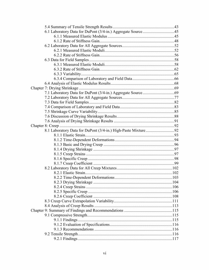
Figure 2.1: AASHTO and ACI 318 Estimated Elastic Moduli
The figure shows that the two models are nearly identical and that the AASHTO LRFD
predicts values for the elastic modulus that are approximately 1 percent higher than the values
suggested by ACI 318. This small difference results from rounding of the ACI 318
specifications (Section 8.5.1) for normal weight concrete (145 pounds per cubic foot). The
differences between the two equations are small, so this research concerned itself only with the
validity of the AASHTO LRDF specifications.
2,500
3,000
3,500
4,000
4,500
5,000
2,000 3,000 4,000 5,000 6,000 7,000
Elas
tic M
odul
us (k
si)
Compressive Strength (psi)
AASHTO LRDFACI 318
5

Both the AASHTO specifications (Section 5.4.2.4-1) and the ACI 318 specifications
(Section 8.5.1) denote the compressive strength of the concrete mixture as 𝑓′𝑐, which is the
design strength. This is not the correct interpretation of the research based on work by Paul
(1960), which used the average compressive strength, 𝑓�̅�.
The evaluation of the elastic modulus provisions is provided in Chapter 5.
2.4 DRYING SHRINKAGE
AASHTO LRFD specifications (Section 5.4.2.3.3) estimate the drying shrinkage strains
for a concrete sample for a particular drying duration. Equation 2.9 shows the form of the
predictive formula.
εsh = khskskfktd0.48 × 10−3 (Equation 2.9)
where: khs = (2.00 − 0.014H)
ks = �
t26e0.36�V S� � + t
t45 + t
� �1064 − 94�V
S� �923
�
kf = 51+fʹci
ktd = � t61−4fʹci+t
�
H = relative humidity (percent)
V/S = volume-to-surface ratio (in.)
fʹci = specified compressive strength of the concrete at the time of initial loading
or prestressing; if the concrete age at the time of initial loading is unknown, it
may be taken as 0.80fʹc.
ACI 209R-92 specifications (2-7) suggest a method of normalizing and fitting drying
shrinkage and creep strain data over time. The equation fits a curve to the shrinkage data by
optimizing two constants, denoted as f and εult. and shown in Equation 2.10.
εtime = time𝛼
(f+time𝛼) × εult. (Equation 2.10)
6

where: α = recommended as 0.90 to 1.10 f = time (in days), recommended as 20 to 130 days.
εult. = The ultimate strain the drying shrinkage samples are expected to reach if left alone to dry indefinitely.
A small modification to Equation 2.10 and the assumption α is 1.0 generates more
meaningful results from the optimized constants. Equation 2.11 shows the predictive equation
with the defined constants from Equation 2.10.
εtime = time(t50+time) × εult. (Equation 2.11)
where: t50 = The time (in days) for the curve to reach 50 percent of the ultimate value εult. = The ultimate strain the drying shrinkage samples are expected to reach if left alone to dry indefinitely.
2.5 CREEP
The creep strain is defined as the time-dependent, load-induced strain from a sustained
loading applied to concrete samples. Creep strain is determined by subtracting the elastic and
drying shrinkage strains from the measured strains of an unsealed, loaded cylinder. The strains
from the drying shrinkage and creep cylinders (sealed and unsealed) were fit to Equation 2.11 to
model the behavior of the strain over time for the different types of cylinders.
The creep coefficient is defined as the creep strains for a mixture divided by the average
elastic strain value. AASHTO LRFD (Section 5.4.2.3.2) defines an equation for estimating the
creep coefficient of a mixture over time, which has the form shown in Equation 2.12.
Ψ (t, ti) = 1.9kskhckfktdti−0.118 (Equation 2.12)
where: ks = 1.45 - 0. 13(V/S) ≥ 1.0
khc = 1.56 - 0.008H
kf = 5
1 + f′ci
ktd = �t
61 − 4f′ci + t�
ti = time cured (days) when load was applied
V/S = volume-to-surface ratio (in)
7

H = relative humidity (percent)
fʹci = specified compressive strength of the concrete at the time of initial loading
or prestressing; if the concrete age at the time of initial loading is unknown, it
may be taken as 0.80f′c.
8

Chapter 3: Test Program
The initial phase of the project was to sample Class 4000 concrete mixtures from five
WSDOT bridge construction projects located throughout Washington State. Coarse aggregate
from each of the WSDOT projects was then acquired to cast laboratory mixtures with a variety
of mix proportions.
The following sections identify the locations of the WSDOT project sites and aggregate
pits that were sampled (Section 3.1), the laboratory mixture proportions (Section 3.2), the types
of tests that were performed and their schedules (Section 3.3), and the procedures followed to
conduct each test (Section 3.4).
3.1 WSDOT PROJECTS SAMPLED
Class 4000 mixtures on bridge construction projects were sampled at five locations
around Washington State. Table 3.1 describes the projects that were sampled and identifies the
WSDOT administrative region for each project. Figure 3.1 shows the location of each
construction site and WSDOT’s six regions.
Table 3.1: Description of WSDOT Projects Sampled
Project Name City Aggregate Name
Pit Name
Project Number
Project Region
Alaskan Way Viaduct Seattle DuPont
(3/4”) B-335 C7847 Northwest
SR 522, Snohomish Snohomish DuPont
(3/4”) B-355 C8128 Northwest
US 395, Freya to Farewell Spokane Sullivan
Road C-173 C7967 Eastern
US 2, Tumwater Canyon Wenatchee Rock
Island DO-209 C8139 North
Central SR 14,
Camas/Washougal Washougal Santosh OR-27 C8105 Southwest
9
Figure 3.2 Locations of WSDOT Projects Sampled
Following the UW sampling, WSDOT staff cast additional compression cylinders at
subsequent dates (in most cases, additional sets of samples were taken on five days) at the field
sites to allow the research team to measure the day-to-day variability of the field mixtures.
3.2 LABORATORY MIXTURES
Four coarse aggregate sources used in the Class 4000 concrete mixtures at five of the
projects were collected for further laboratory testing. The Alaskan Way Viaduct and SR 522
Snohomish projects used the same aggregate pit (DuPont [3/4-in.]). Three additional coarse
aggregate sources were sampled for this research. One of the additional coarse aggregates was a
pea gravel to measure the effects of decreasing the aggregate size. A second aggregate source
was selected to sample the South Central region of Washington State. The third additional
aggregate source (Okanogan Valley) was sampled from the North Central Region. Table 3.2 lists
the aggregate sources sampled for this project, and Figure 3.2 shows the location of each
aggregate pit.
10

Table 3.2: Aggregate Sources Sampled
Aggregate Name Pit Number WSDOT Region DuPont (3/4”) B-335 Olympic DuPont (3/8”) B-335 Olympic Sullivan Road C-173 Eastern
Okanogan Valley U-119 North Central Rock Island DO-209 North Central
Pasco FN-50 South Central Santosh OR-27 Oregon Region 1
Figure 3.3: Locations of Aggregate Sources Sampled
For each aggregate source, laboratory mixtures were proportioned to produce four
mixtures (high and low paste contents, as well as high and low strengths) at levels expected to
cover the extreme ranges of paste contents and water-cementitious ratios for a 4,000 psi design
mixture. The collected aggregate sources were tested for absorption and specific gravity (ASTM
C127) to account for the moisture content and maintain a constant coarse-to-fine aggregate ratio.
For all of the mixtures, the coarse-to-fine aggregate ratio was 0.60, an air content of 5 percent
11
was maintained by including an air entraining admixture, and cement Type I/II was used for
casting.
Table 3.3 lists the proportions of the conventional laboratory mixtures. The pea gravel
[DuPont (3/8-in.)] required alterations to the mix proportions to account for the smaller
aggregate size and can be seen in Table 3.4.
Table 3.3: Conventional Laboratory Concrete Mixture Proportions
Mixture Paste Content (%) Cement Factor Water-Cementitious
Ratio High Paste 30.5 7.9 0.38 Low Paste 24.0 6.2 0.38 High Strength 27.0 7.9 0.30 Low Strength 27.0 6.1 0.49
Table 3.4: Pea Gravel Laboratory Concrete Mixture Proportions
Mixture Paste Content (%) Cement Factor Water-Cementitious Ratio High Paste 33.2 8.5 0.38 Low Paste 26.1 6.7 0.38 High Strength 28.2 7.8 0.33 Low Strength 29.3 6.5 0.49
3.3 TESTS PERFORMED
Six standardized tests (compressive strength, flexural strength, split-tension strength,
elastic modulus, drying shrinkage, and creep) were conducted to characterize the hardened
properties of each laboratory concrete mixture. The testing regime for each of the performed
tests is listed in Table 3.5 for the laboratory mixtures and in Table 3.6 for the field samples.
12

Table 3.5: Testing Schedule for Laboratory Mixtures
Laboratory Mixtures
Test Performed Day 7 Day 14
Day 28
Day 56
Compressive Strength X X X X
Elastic Modulus X X X X Drying Shrinkage (Test Start Date) X
Creep (Test Start Date) X
Table 3.6: Testing Schedule for Field Samples
Initial Field Sampling Field Variability
Test Performed Day 7 Day 14
Day 28
Day 56
Day 7
Day 14
Day 28
Day 56
Compressive Strength X X X X X
Elastic Modulus X X X X X Split Tension Strength X X
Flexure Strength X X Drying Shrinkage (Test Start Date) X
3.4 SPECIMEN PREPARATION AND TESTING
The standardized procedures followed to prepare and test concrete samples for each of
the six tests are described in the following subsections.
3.4.1 Compressive Strength Test Procedure
The compressive strength tests were performed on 6-in. x 12–in. concrete cylinders that
were cast per ASTM C192 procedures. Compression cylinders from laboratory mixtures were
cast with reusable steel molds, whereas the field cylinders were cast with single-use plastic
molds.
13
Upon removal of the concrete cylinders from the molds, the samples were immediately
capped with a sulfur-based compound following the ASTM C617-specified procedure. The
cylinders were then stored in a moisture room (as defined by ASTM C192) until the respective
cure duration had passed. Compression tests were performed on a minimum of two concrete
samples; three samples were used if the failure load varied by more than 5 percent between the
two cylinders. The procedure followed to conduct the compression tests is defined in ASTM
C39.
3.4.2 Tensile Strength Test Procedure
Split-tension tests were performed on 6-in. x 12–in. cylinders, and flexural strength
samples were cast as 6-in. x6-in. x21-in. beams following the ASTM C192 procedure. The
concrete cylinders and beam samples for the tensile strength tests were cast only from field
mixtures. The beam samples were cast in reusable steel molds, and the cylinder samples were
cast in single-use plastic molds. The samples were allowed to cure for 16 hours onsite before
they were transported back to the University of Washington. The concrete samples were left in
the molds during transportation to reduce the possibility of damaging the samples.
Upon arrival at the university, the concrete cylinders and beams were removed from the
molds and stored in the moisture room to cure until the test date. Split-tension tests were
performed on two cylinders after curing for 28 and 56 days following ASTM C496. Flexure tests
were performed by the third-point loading method as defined in ASTM C78, on three beam
samples after curing for 28 and 56 days.
3.4.3 Elastic Modulus Test Procedure
For the field and laboratory mixtures, two additional 6-in. x 12–in. cylinders were cast,
following ASTM C192 procedures, to test the elastic modulus. The cylinders were capped with
the sulfur-based compound, per ASTM C617, upon removal from the molds. The samples were
stored in the same moisture room as the compression cylinders. On each test date, the elastic
moduli of the two cylinders were measured in accordance with ASTM C469: the cylinders were
loaded to 50 percent of the failure load and unloaded for two cycles. The elastic modulus
14
cylinders were then placed back in the moisture room to continue curing until the following
testing date.
The applied load and deformation of the cylinder were recorded for 1-second intervals.
The load and deformation were then converted into stress and strain values. The elastic modulus
was determined by fitting the stress and strain data from 50 microstrain to 40 percent of the
failure stress for the mixture at that test date.
3.4.4 Drying Shrinkage Test Procedure
The drying shrinkage was monitored for field and laboratory mixtures. Three beam
samples were cast from each mixture that were 3 in. x 4 in. x 16 in., as per ASTM C157, in
reusable steel molds. The concrete beams were removed from the molds after curing for 16 to 24
hours. Upon removal, the shrinkage samples were stored in a saturated Calcium Hydroxide water
bath for curing the first 28 days.
On Day 28 of curing, the beams were removed from the water and towel dried to
saturated surface-dry conditions. The weight and length of each beam was measured twice to
establish an initial length and weight. The samples were then set inside a temperature controlled
room, as defined by ASTM C157, and began air drying. The monitoring schedule for the
shrinkage beams was to then measure the weight and length of the beams once a day for the first
week, then once a week for the first month, and then once a month for the first year of air drying.
3.4.5 Creep Test Procedure
Creep testing was performed on laboratory high- and low-paste mixtures. Three distinct
aggregate sources were selected for the creep testing. For each mixture, six additional concrete
cylinder samples were cast from the mixture. These cylinders were cast in reusable steel molds
and prepared for the creep rigs by applying the sulfur-based capping compound as per ASTM
C617, upon removal from the molds. The six creep cylinders were then stored in the moisture
room to cure.
Two cylinders were removed from the moisture room on the twelfth day of curing. The
surface of these samples was dried and coated with an epoxy sealant. The sealant was allowed to
harden for 24 hours before a second epoxy coat was applied on Day 13. This second coat was
15
allowed to harden for another 24 hours. Once the two sealed cylinders had finished drying on
Day 14, the remaining four creep cylinders were taken out of the moisture room and the surfaces
were allowed to dry. All six of the creep cylinders were placed on a wooden rack, and steel
gauge studs were epoxied onto each of the cylinders’ side. The studs were placed at 10-inch
spaces along the length of each cylinder. The cylinders were then rotated 90 degrees, and another
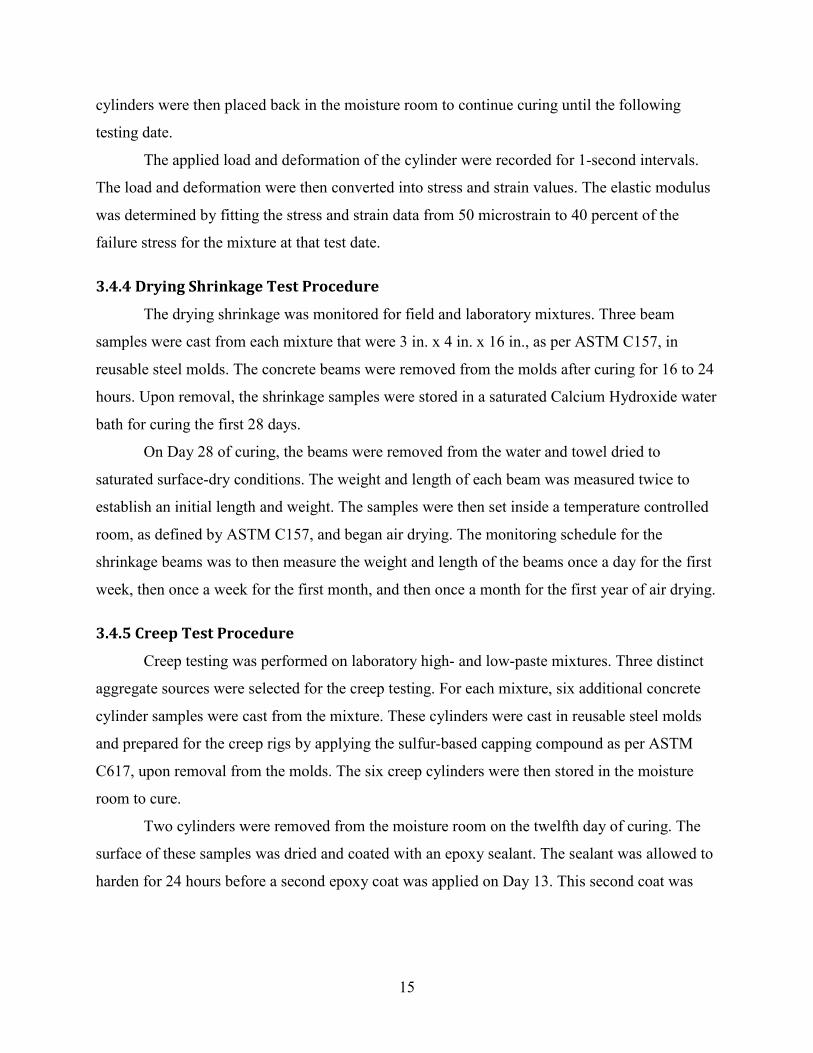
set of studs was glued onto the side of the cylinder. This process was repeated until the cylinders
had studs placed on each quadrant. A picture of the creep cylinders with the attached gauge studs
can be seen in Figure 3.3.
Figure 3.4: Gauge Stud Placement on Typical Creep Cylinder
10” Length
16

The creep cylinder ends were capped with sulfur, so the rigs were assembled by stacking
four cylinders (two sealed and two non-sealed) overtop each other. The remaining two non-
sealed cylinders were placed adjacent to the creep rig. These two cylinders were used to measure
the drying shrinkage for the creep samples. Figure 3.4 shows a typical creep rig set-up, with a
non-sealed cylinder at the bottom of the stack and sealed and non-sealed cylinders stacked
interchangeably.
Figure 3.5: Typical Creep Rig Assembly
Sealed Creep
Unsealed Creep
17
Once the creep rig had been assembled, measurements for each of the six cylinders were
taken. These measurements were repeated until a consistent initial length for each set of gauge
studs was determined. The creep rig was then loaded with a hydraulic ram to a target load of 35
percent of the Day 14 failure stress. This failure stress was determined from the mixture’s
compression test performed on alternative samples. The lengths of the four creep cylinders were
measured while the loading from the hydraulic ram was still applied. Locking nuts were
tightened to maintain the applied load on the creep rig once the pressure had been released from
the ram. The lengths of the creep cylinders were measured a final time once the load from the
ram had been removed.
This measurement and loading procedure was repeated for each monitor date. The
schedule for monitoring each creep rig was twice on the first day of assembly, followed by once
a day for the first week, then once a week for the first month, and then once a month for the
following year.
18
Chapter 4: Compressive Strength
The compressive strength of concrete is strongly correlated with other properties. This
chapter discusses the compressive strengths of the concrete mixtures used in this study, as well
as the effects of time, water-cementitious ratio, paste content, and coarse aggregate. The
influence of these factors on strength variability is also examined.
A single laboratory aggregate source is discussed in Section 4.1 to illustrate the data-
analysis procedure. Section 4.2 summarizes the results for the remaining aggregate sources and
identifies trends. The field mixture data are presented in Section 4.3. The results from all of the
compressive strength tests are reported in Appendix A.
4.1 LABORATORY DATA FOR DUPONT (3/4-IN.) AGGREGATE SOURCE
The DuPont ¾-inch aggregate is discussed in detail, since two of the sampled WSDOT
projects used this aggregate. The three-quarter inch designation in the naming system for DuPont
denotes the maximum aggregate size. The size was included in the aggregate designation to
distinguish it from the pea gravel (3/8-in. max size) from the same pit location that was also
considered in this research.
4.1.1 Measured Compressive Strengths
As mentioned in Section 2.3, compressive tests were performed on lab mixtures at days
7, 14, 28, and 56. The compressive strengths for the four DuPont (3/4-in.) laboratory mixtures
(high paste, low paste, high strength, low strength), along with the mixture proportions, are
reported in Table 4.1 and Figure 4.1.
19

Table 4.1: Measured Compressive Strengths: DuPont (3/4-in.)
Mixture
Paste Content
(%)
Water-Cementitious
Ratio Day 7 (psi)
Day 14 (psi)
Day 28 (psi)
Day 56 (psi)
High-Paste 30.5 0.38 5,350 4,990 * 6,530 7,020 Low-Paste 24.0 0.38 3,400 3,710 4,400 4,710
High- Strength 27.0 0.30 5,070 5,680 6,040** 7,560 Low-Strength 27.0 0.49 2,840 3,210 3,750 4,000
* Day 14: High Paste mixture had low break, not used to fit EQ 2.1 ** Day 28: High Strength mixture had low break, best-fit value used for calibrating EQ 2.1
Figure 4.1: Compressive Strengths: DuPont (3/4-in.) Mixtures
The compressive strength of the mixtures at Day 28 ( f2̅8 ) ranged from 3,750 psi to 6,530
psi. By Day 56, the strengths of all mixtures had reached or exceeded the design strength of
4,000 psi. The compressive strengths of the high-paste and high-strength mixtures were similar.
The low-paste and low-strength mixtures also had strengths similar to each other. These two
mixtures had strengths approximately 2,000 psi lower than the strength of the high-paste and
high-strength mixtures.
0
1,000
2,000
3,000
4,000
5,000
6,000
7,000
8,000
0 10 20 30 40 50 60
Com
pres
sive
Str
engt
h (p
si)
Age (days)
High Paste
Low Paste
High Strength
Low Strength
20
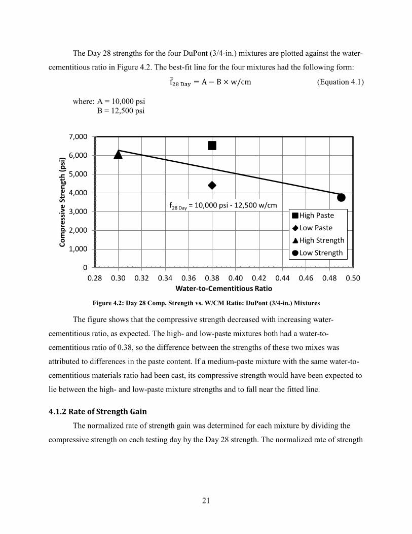
The Day 28 strengths for the four DuPont (3/4-in.) mixtures are plotted against the water-
cementitious ratio in Figure 4.2. The best-fit line for the four mixtures had the following form:
f2̅8 Day = A − B × w/cm (Equation 4.1) where: A = 10,000 psi B = 12,500 psi
Figure 4.2: Day 28 Comp. Strength vs. W/CM Ratio: DuPont (3/4-in.) Mixtures
The figure shows that the compressive strength decreased with increasing water-
cementitious ratio, as expected. The high- and low-paste mixtures both had a water-to-
cementitious ratio of 0.38, so the difference between the strengths of these two mixes was
attributed to differences in the paste content. If a medium-paste mixture with the same water-to-
cementitious materials ratio had been cast, its compressive strength would have been expected to
lie between the high- and low-paste mixture strengths and to fall near the fitted line.
4.1.2 Rate of Strength Gain
The normalized rate of strength gain was determined for each mixture by dividing the
compressive strength on each testing day by the Day 28 strength. The normalized rate of strength
f28 Day = 10,000 psi - 12,500 w/cm
0
1,000
2,000
3,000
4,000
5,000
6,000
7,000
0.28 0.30 0.32 0.34 0.36 0.38 0.40 0.42 0.44 0.46 0.48 0.50
Com
pres
sive
Str
engt
h (p
si)
Water-to-Cementitious Ratio
High PasteLow PasteHigh StrengthLow Strength
21

gain for each of the four testing days was then fit to a curve in the form of Equation 2.1, as
explained in Section 2.1.
For the DuPont (3/4-in.) low-paste mixture, the results from the four compression testing
days were evaluated to determine the K1 and K2 constants in Equation 2.1. The resulting optimal
values are provided in Equation 4.2, and the fitted curve is plotted in Figure 4.3. The normalized
compressive strength data are also shown in the figure to show the goodness of fit.
DuPont (3/4 − in. ) Low − Paste: ftimef2̅8� =
time(3.22 + 0.89 × time) (Equation 4.2)
Figure 4.3: Rate of Strength Gain Fitted Curve: DuPont (3/4-in.) Low-Paste Mixture
This procedure was repeated for the other three DuPont (3/4-in.) mixtures. The low break
for Day 14 of the high-paste mixture was excluded from the data set when K1 and K2 were fit.
The low break for Day 28 of the high-strength mixture was accounted for by excluding the Day
28 break from the data set and optimizing K1 and K2 by normalizing to the Day 56 strength.
With the normalized fitted curve for the high-strength mixture, the strength at Day 28 was
estimated by the value provided from the curve.
0.0
0.2
0.4
0.6
0.8
1.0
1.2
0 10 20 30 40 50 60
Nor
mal
ized
Stre
ngth
(f ti
me/
f 28)
Time (days)
Low Paste
Fitted Curve
22

The constants for the four fitted curves are listed in Table 4.2, along with the mean
compressive strength at Day 28 for each mixture. Figure 4.4 shows the four fitted curves for the
DuPont (3/4-in.) laboratory mixtures.
Table 4.2: Optimized Constants for DuPont (3/4-in.) Aggregate
Mixture 𝐟𝐟�̅�𝟖 (psi) K1 K2 𝐟𝐟�̅�𝟕/𝐟𝐟�̅�𝟖 𝐟𝐟�̅�𝟔𝟔/𝐟𝐟�̅�𝟖 High-Paste 6,530 2.23 0.91 0.82 1.07 Low-Paste 4,400 3.23 0.89 0.77 1.07
High-Strength 6,740* 3.64 0.87 0.77 1.09 Low-Strength 3,750 3.26 0.89 0.76 1.07
Average 5,360 3.09 0.89 0.78 1.08
St. Deviation 1,500 0.60 0.02 0.03 0.01 Coef. of Variation 28.1% 19.5% 1.7% 3.9% 0.7%
* Determined from fitted curve
Figure 4.4: Rate of Strength Gain Fitted Curves: DuPont (3/4-in.) Mixtures
The ratio of the Day 7 strength to the Day 28 strength was nearly identical for the low-
paste, high-strength, and low-strength mixtures. At Day 7, the mean compressive strength for
these three mixtures was on average 77.5 percent of the 28 day strength. The high-paste mixture
gained strength slightly more rapidly. The same ratio for the high-paste mixture was 81.9
0.0
0.2
0.4
0.6
0.8
1.0
1.2
0 10 20 30 40 50 60
Nor
mal
ized
Stre
ngth
(ftim
e/f 2
8)
Age (days)
High PasteLow PasteHigh StrengthLow Strength
23
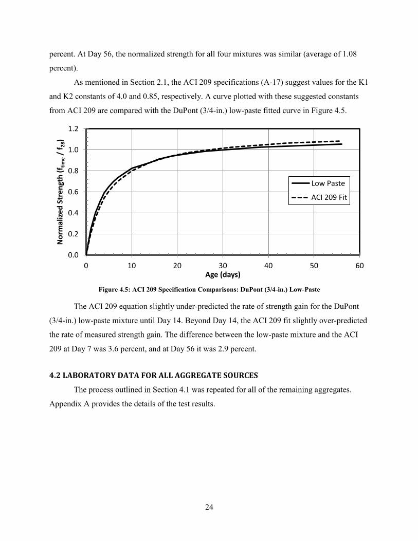
percent. At Day 56, the normalized strength for all four mixtures was similar (average of 1.08
percent).
As mentioned in Section 2.1, the ACI 209 specifications (A-17) suggest values for the K1
and K2 constants of 4.0 and 0.85, respectively. A curve plotted with these suggested constants
from ACI 209 are compared with the DuPont (3/4-in.) low-paste fitted curve in Figure 4.5.
Figure 4.5: ACI 209 Specification Comparisons: DuPont (3/4-in.) Low-Paste
The ACI 209 equation slightly under-predicted the rate of strength gain for the DuPont
(3/4-in.) low-paste mixture until Day 14. Beyond Day 14, the ACI 209 fit slightly over-predicted
the rate of measured strength gain. The difference between the low-paste mixture and the ACI
209 at Day 7 was 3.6 percent, and at Day 56 it was 2.9 percent.
4.2 LABORATORY DATA FOR ALL AGGREGATE SOURCES
The process outlined in Section 4.1 was repeated for all of the remaining aggregates.
Appendix A provides the details of the test results.
0.0
0.2
0.4
0.6
0.8
1.0
1.2
0 10 20 30 40 50 60
Nor
mal
ized
Stre
ngth
(ftim
e / f 2
8)
Age (days)
Low Paste
ACI 209 Fit
24
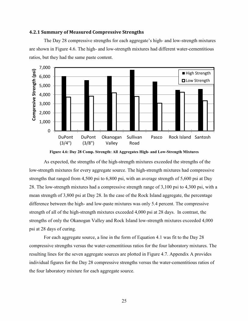
4.2.1 Summary of Measured Compressive Strengths
The Day 28 compressive strengths for each aggregate’s high- and low-strength mixtures
are shown in Figure 4.6. The high- and low-strength mixtures had different water-cementitious
ratios, but they had the same paste content.
Figure 4.6: Day 28 Comp. Strength: All Aggregates High- and Low-Strength Mixtures
As expected, the strengths of the high-strength mixtures exceeded the strengths of the
low-strength mixtures for every aggregate source. The high-strength mixtures had compressive
strengths that ranged from 4,500 psi to 6,800 psi, with an average strength of 5,600 psi at Day
28. The low-strength mixtures had a compressive strength range of 3,100 psi to 4,300 psi, with a
mean strength of 3,800 psi at Day 28. In the case of the Rock Island aggregate, the percentage
difference between the high- and low-paste mixtures was only 5.4 percent. The compressive
strength of all of the high-strength mixtures exceeded 4,000 psi at 28 days. In contrast, the
strengths of only the Okanogan Valley and Rock Island low-strength mixtures exceeded 4,000
psi at 28 days of curing.
For each aggregate source, a line in the form of Equation 4.1 was fit to the Day 28
compressive strengths versus the water-cementitious ratios for the four laboratory mixtures. The
resulting lines for the seven aggregate sources are plotted in Figure 4.7. Appendix A provides
individual figures for the Day 28 compressive strengths versus the water-cementitious ratios of
the four laboratory mixture for each aggregate source.
0
1,000
2,000
3,000
4,000
5,000
6,000
7,000
DuPont(3/4")
DuPont(3/8")
OkanoganValley
SullivanRoad
Pasco Rock Island Santosh
Com
pres
ive
Stre
ngth
(psi
)
High Strength
Low Strength
25
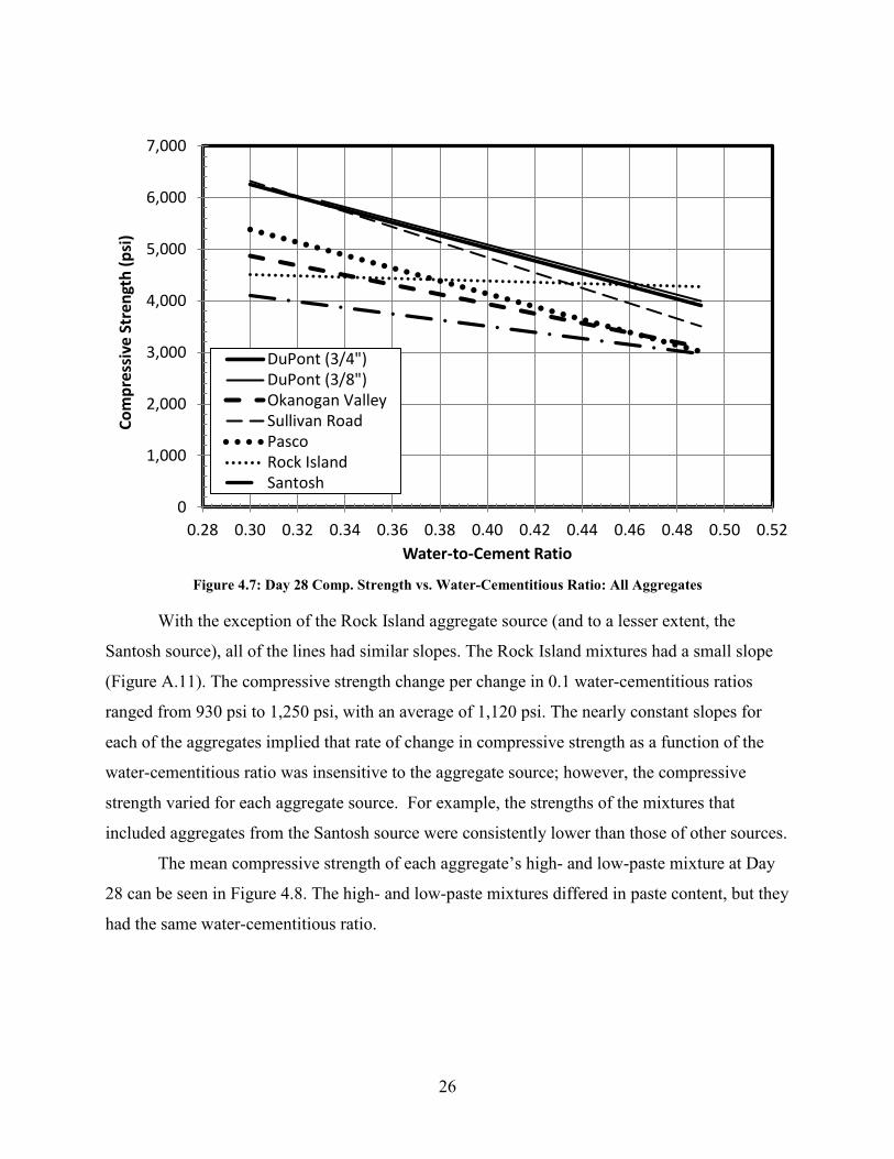
Figure 4.7: Day 28 Comp. Strength vs. Water-Cementitious Ratio: All Aggregates
With the exception of the Rock Island aggregate source (and to a lesser extent, the
Santosh source), all of the lines had similar slopes. The Rock Island mixtures had a small slope
(Figure A.11). The compressive strength change per change in 0.1 water-cementitious ratios
ranged from 930 psi to 1,250 psi, with an average of 1,120 psi. The nearly constant slopes for
each of the aggregates implied that rate of change in compressive strength as a function of the
water-cementitious ratio was insensitive to the aggregate source; however, the compressive
strength varied for each aggregate source. For example, the strengths of the mixtures that
included aggregates from the Santosh source were consistently lower than those of other sources.
The mean compressive strength of each aggregate’s high- and low-paste mixture at Day
28 can be seen in Figure 4.8. The high- and low-paste mixtures differed in paste content, but they
had the same water-cementitious ratio.
0
1,000
2,000
3,000
4,000
5,000
6,000
7,000
0.28 0.30 0.32 0.34 0.36 0.38 0.40 0.42 0.44 0.46 0.48 0.50 0.52
Com
pres
sive
Str
engt
h (p
si)
Water-to-Cement Ratio
DuPont (3/4")DuPont (3/8")Okanogan ValleySullivan RoadPascoRock IslandSantosh
26
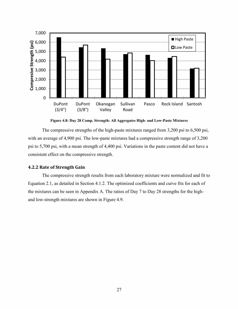
Figure 4.8: Day 28 Comp. Strength: All Aggregates High- and Low-Paste Mixtures
The compressive strengths of the high-paste mixtures ranged from 3,200 psi to 6,500 psi,
with an average of 4,900 psi. The low-paste mixtures had a compressive strength range of 3,200
psi to 5,700 psi, with a mean strength of 4,400 psi. Variations in the paste content did not have a
consistent effect on the compressive strength.
4.2.2 Rate of Strength Gain
The compressive strength results from each laboratory mixture were normalized and fit to
Equation 2.1, as detailed in Section 4.1.2. The optimized coefficients and curve fits for each of
the mixtures can be seen in Appendix A. The ratios of Day 7 to Day 28 strengths for the high-
and low-strength mixtures are shown in Figure 4.9.
0
1,000
2,000
3,000
4,000
5,000
6,000
7,000
DuPont(3/4")
DuPont(3/8")
OkanoganValley
SullivanRoad
Pasco Rock Island Santosh
Com
pres
ive
Stre
ngth
(psi
) High Paste
Low Paste
27

Figure 4.9: Rate of Strength Gain: All Aggregates High- and Low-Strength Mixtures
The rate of strength gains for the high-strength mixtures consistently exceeded the rate of
strength gains for the low-strength mixtures. Since the paste contents were constant, the
difference in rate of strength gains between the high- and low-strength mixtures was attributed to
the effect of the water-cementitious ratio as well as cement content. The ratio between the high
and low strength mixture’s rate of strength gain had a range of 1.09 to 1.22 with a mean of 1.16.
The ratio of Day 7 to Day 28 strengths for each of the high-and low-paste mixtures can
be seen in Figure 4.10. The high-and low-paste mixtures had the same water-cementitious ratio
with only variations in the paste content.
0.0
0.2
0.4
0.6
0.8
1.0
DuPont(3/4")
DuPont(3/8")
OkanoganValley
SullivanRoad
Pasco Rock Island Santosh
Rate
of S
tren
gth
Gai
n (f 7
/f28
) High StrengthLow Strength
28

Figure 4.10: Rate of Strength Gain: All Aggregates High- and Low-Paste Mixtures
The Day 7 rate of strength gain for the high-paste mixtures ranged from 0.79 to 0.88,
with a mean normalized strength of 0.83. The low-strength mixtures had a rate of strength gain
that ranged from 0.77 to 0.90, with an average rate of 0.82. There were no consistent differences
between the normalized rates of strength gain for the high- and low-paste mixtures.
4.3 DATA FOR FIELD SAMPLES
This section discusses the results from the compressive tests performed on the field
samples for each of the five WSDOT projects.
4.3.1 Measured Compressive Strengths
The compressive strengths for all five of the WSDOT projects collected by the UW are
reported in Table 4.3 and in Figure 4.11. Table 4.3 also lists the paste content and water-
cementitious ratio for the mixture sampled at each project. The Tumwater Canyon project was
the only construction job that included fly ash in the mixture. The reported paste content includes
the converted fly ash as a component of cement.
0.0
0.2
0.4
0.6
0.8
1.0
DuPont(3/4")
DuPont(3/8")
OkanoganValley
SullivanRoad
Pasco Rock Island Santosh
Rate
of S
tren
gth
Gai
n (f 7
/f28
) High Paste Low Paste
29

Table 4.3: Field Sample Compressive Strengths
Project Aggregate Name
Paste Content
(%)
W/CM Ratio
Day 7 (psi)
Day 14 (psi)
Day 28 (psi)
Day 56 (psi)
Freya to Farewell
Sullivan Road 25.5 0.31 4,650 5,180 5,420 5,900
Alaskan Way
DuPont (3/4") 25.2 0.31 4,250 5,010 5,290 5,660
Tumwater Canyon
Rock Island 25.9* 0.40* 3,030 3,670 3,680** 4,410
Snohomish DuPont (3/4") 24.6 0.32 5,090 5,700 6,300 6,370
Camas / Washougal Santosh 27.8 0.41 3,020 3,420 4,070 4,380
* Wenatchee mixture included fly ash ** Day 28: Wenatchee mixture had low break, best-fit value used for calibrating EQ 2.1
Figure 4.11: Field Sample Compressive Strength over Time
The compressive strengths of the Tumwater Canyon and Camas/Washougal project
concrete were similar, whereas the Freya to Farewell, Alaskan Way, and Snohomish projects all
had compressive strengths that were around 2,000 psi higher. The Day 28 compressive strength
0
1,000
2,000
3,000
4,000
5,000
6,000
7,000
0 10 20 30 40 50 60
Com
pres
sive
Str
engt
h (p
si)
Time (days)
Freya to FarewellAlaskan WayTumwater CanyonSnohomishCamas / Washougal
30
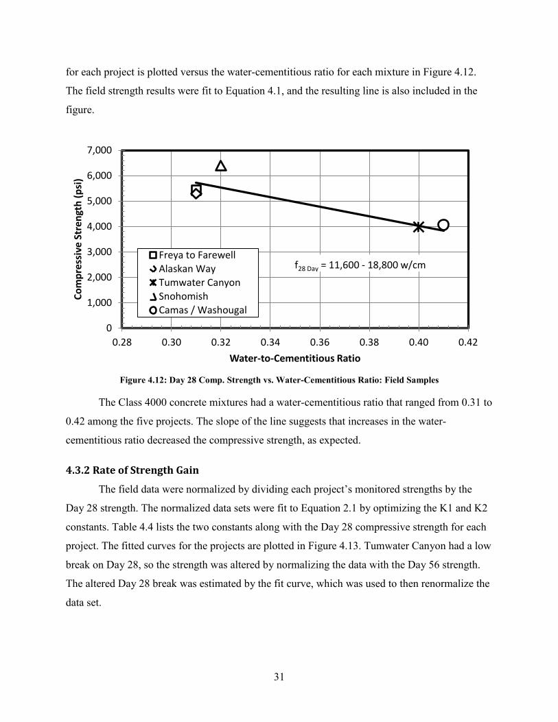
for each project is plotted versus the water-cementitious ratio for each mixture in Figure 4.12.
The field strength results were fit to Equation 4.1, and the resulting line is also included in the
figure.
Figure 4.12: Day 28 Comp. Strength vs. Water-Cementitious Ratio: Field Samples
The Class 4000 concrete mixtures had a water-cementitious ratio that ranged from 0.31 to
0.42 among the five projects. The slope of the line suggests that increases in the water-
cementitious ratio decreased the compressive strength, as expected.
4.3.2 Rate of Strength Gain
The field data were normalized by dividing each project’s monitored strengths by the
Day 28 strength. The normalized data sets were fit to Equation 2.1 by optimizing the K1 and K2
constants. Table 4.4 lists the two constants along with the Day 28 compressive strength for each
project. The fitted curves for the projects are plotted in Figure 4.13. Tumwater Canyon had a low
break on Day 28, so the strength was altered by normalizing the data with the Day 56 strength.
The altered Day 28 break was estimated by the fit curve, which was used to then renormalize the
data set.
0
1,000
2,000
3,000
4,000
5,000
6,000
7,000
0.28 0.30 0.32 0.34 0.36 0.38 0.40 0.42
Com
pres
sive
Str
engt
h (p
si)
Water-to-Cementitious Ratio
Freya to FarewellAlaskan WayTumwater CanyonSnohomishCamas / Washougal
f28 Day = 11,600 - 18,800 w/cm
31

Table 4.4: Predictive Equation Constants for Field Samples
Project 𝐟𝐟�̅�𝟖 (psi) K1 K2 𝐟𝐟�̅�𝟕/𝐟𝐟�̅�𝟖 𝐟𝐟�̅�𝟔𝟔/𝐟𝐟�̅�𝟖 Freya to Farewell 5,420 1.88 0.90 0.84 1.06 Alaskan Way 5,290 2.42 0.90 0.80 1.07 Tumwater Canyon 3,980** 3.26 0.86 0.76 1.01 Snohomish 6,300 2.22 0.94 0.80 1.08 Camas / Washougal 4,070 3.70 0.87 0.74 1.08
Average 4,970 2.69 0.89 0.79 1.06 St. Deviation 1,100 0.76 0.03 0.04 0.03 Coef. Of Variation 22.1% 28.2% 3.7% 4.6% 2.6%
** Day 28: Wenatchee had a low break. Best-fit value estimated
Figure 4.13: Rate of Strength Gain Fitted Curves: Field Samples
After the first week, the normalized rate of strength gain for the field mixtures had less
than a 5.0 percent coefficient of variation. Despite the field mixtures having large variations in
mixture proportions, aggregate type, and compressive strengths, only the initial rate of strength
gain varied among them. These variations in the initial strength gain were to be expected, given
the analysis of figures 4.9 and 4.10. The initial rate of strength gain increased with decreasing
water-cementitious ratios. The field mixture proportions ranged from a water-cementitious ratio
0.0
0.2
0.4
0.6
0.8
1.0
1.2
0 10 20 30 40 50 60
Nor
mal
ized
Stre
ngth
(f7/
f 28)
Age (days)
Freya to FarewellAlaskan WayTumwater CanyonSnohomishCamas / Washougal
32
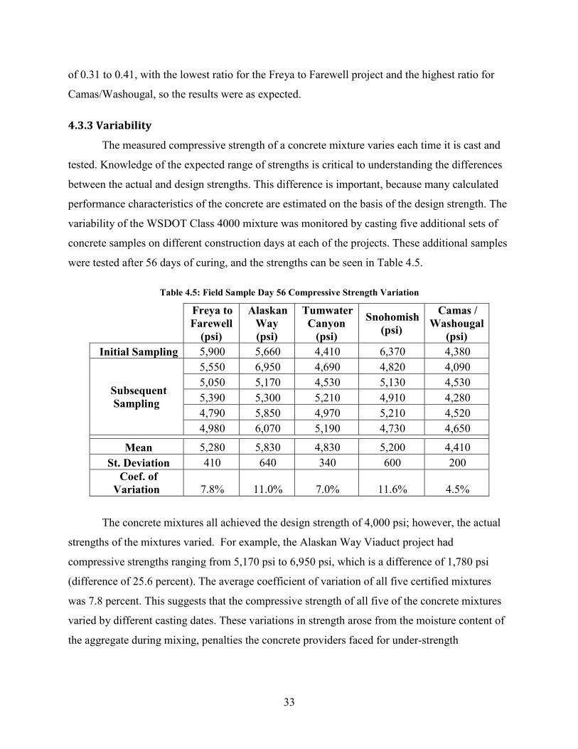
of 0.31 to 0.41, with the lowest ratio for the Freya to Farewell project and the highest ratio for
Camas/Washougal, so the results were as expected.
4.3.3 Variability
The measured compressive strength of a concrete mixture varies each time it is cast and
tested. Knowledge of the expected range of strengths is critical to understanding the differences
between the actual and design strengths. This difference is important, because many calculated
performance characteristics of the concrete are estimated on the basis of the design strength. The
variability of the WSDOT Class 4000 mixture was monitored by casting five additional sets of
concrete samples on different construction days at each of the projects. These additional samples
were tested after 56 days of curing, and the strengths can be seen in Table 4.5.
Table 4.5: Field Sample Day 56 Compressive Strength Variation
Freya to Farewell
(psi)
Alaskan Way (psi)
Tumwater Canyon
(psi)
Snohomish (psi)
Camas / Washougal
(psi) Initial Sampling 5,900 5,660 4,410 6,370 4,380
Subsequent Sampling
5,550 6,950 4,690 4,820 4,090 5,050 5,170 4,530 5,130 4,530 5,390 5,300 5,210 4,910 4,280 4,790 5,850 4,970 5,210 4,520 4,980 6,070 5,190 4,730 4,650
Mean 5,280 5,830 4,830 5,200 4,410 St. Deviation 410 640 340 600 200
Coef. of Variation 7.8% 11.0% 7.0% 11.6% 4.5%
The concrete mixtures all achieved the design strength of 4,000 psi; however, the actual
strengths of the mixtures varied. For example, the Alaskan Way Viaduct project had
compressive strengths ranging from 5,170 psi to 6,950 psi, which is a difference of 1,780 psi
(difference of 25.6 percent). The average coefficient of variation of all five certified mixtures
was 7.8 percent. This suggests that the compressive strength of all five of the concrete mixtures
varied by different casting dates. These variations in strength arose from the moisture content of
the aggregate during mixing, penalties the concrete providers faced for under-strength
33

performance, and methods of dealing with complications from weather conditions (i.e., using hot
water to speed up the rate of hydration when casting on cold days).
4.4 ANALYSIS OF COMPRESSIVE STRENGTH RESULTS
As expected, the effect of water-cementitious ratio was consistent for the laboratory and
field mixtures (figures 4.2, 4.6, 4.7 and 4.12). Strength decreased as the water-cementitious ratio
increased. The variation in strength as a function of the water-cementitious ratio was not constant
for each aggregate source (Figure 4.7). The Rock Island and Santosh aggregate sources were less
sensitive to modifications to the water-cementitious ratio, so making higher-strength concrete
with these aggregate types might be more difficult. The effect of the water-cementitious ratio on
the rate of strength gain (Day 7 to Day 28 strength ratio) was consistent for the aggregates
(Figure 4.9); the higher-strength mixtures had a higher rate of strength ratio than the lower-
strength mixtures.
The compressive strength and rate of strength gain appeared to be insensitive to
variations in the paste content. This may have been due to differences in stiffness between coarse
aggregates and paste. Stiffer aggregates (DuPont [3/4-in.]) achieve higher strength with higher
paste contents, while less stiff aggregates (Sullivan Road) can achieve better strength with less
paste. The compressive strength for the high-paste mixture was not consistently stronger than the
low-paste mixture for a single aggregate source and water-cementitious ratio (Figure 4.8). The
high-paste mixture’s rate of strength gain for the normalized Day 7 strength did not always
exceed that of the low-paste mixture for a given aggregate (Figure 4.10).
The normalized compressive strength data fit the ACI 209 specifications (A-17, Equation
2.1) well, despite the differences in cement type and changes in the cement refinement process
(figures 4.3 and 4.5). The difference in cement and cement refinement processes was reflected in
the initial rate of strength gain (ratio of Day 7 to Day 28 strengths). ACI 209 recommends values
for the K1 and K2 constants as 4.0 and 0.85, respectively. The optimized K1 and K2 values for
the laboratory data had an average value of 2.4 and 0.90, a difference of 39.0 percent and 5.5
percent, respectively.
34

Chapter 5: Tensile Strength
This chapter discusses flexure and split-tension tests of five field concrete mixtures
sampled in this study. The paste content and water-cementitious ratio varied among the sampled
projects, as seen in Table 5.1. Since only five projects were sampled, it was not possible to
identify the effects of paste content or water-cementitious ratio on tensile strength.
Table 5.1: Field Mixture Proportions
Project Paste Content
(%) Water-Cementitious
Ratio Freya to Farewell 25.5 0.31 Alaskan Way 25.2 0.31 Tumwater Canyon 25.9* 0.40* Snohomish 24.6 0.32 Camas / Washougal 27.8 0.41
* Tumwater Canyon mixture included fly ash.
The tensile and compressive strength results for the field samples for Day 28 and Day 56
are listed in Table 5.2. Section 5.1 and Section 5.2 discuss the flexure test and split-tension test
analysis, respectively. The relationship between the flexure and split-tension strengths is
investigated in Section 5.3.
Table 5.2: Flexural and Compressive Strength Results
Alaskan Way Snohomish Tumwater
Canyon Freya to Farewell
Camas / Washougal
Flexural Strength (psi)
Day 28 780 680 620 830 670 Day 56 820 680 620 850 700
Split-Tension (psi)
Day 28 540 450 390 540 350 Day 56 510 500 350 510 410
Compressive Strength (psi)
Day 28 5,290 6,400 3,680 5,420 3,880 Day 56 5,660 6,470 4,410 5,900 4,380
Table 5.1 lists the Day 28 and 56 strengths for each test. As expected, the flexural and
compressive strengths for the field mixtures increased slightly between Day 28 and Day 56. In
contrast, the split-tensile strengths did not consistently increase with time. For the Alaskan Way,
35
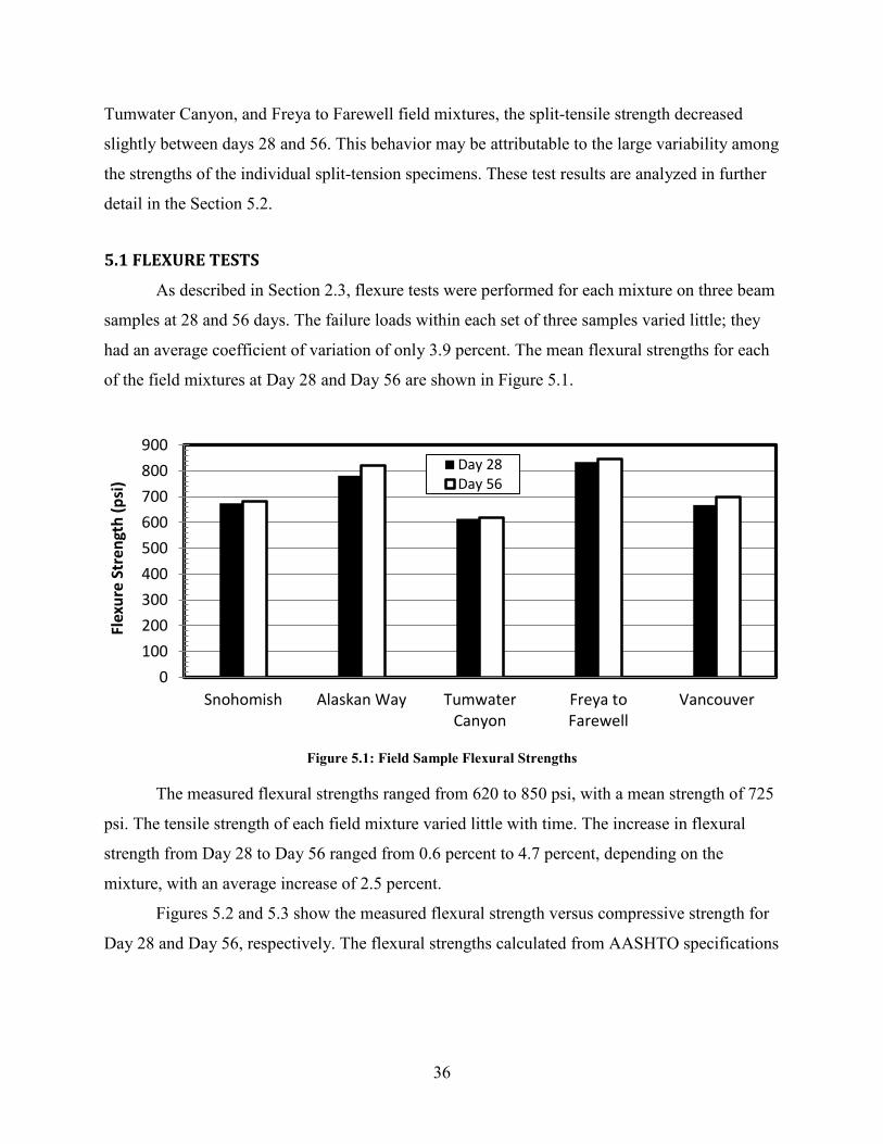
Tumwater Canyon, and Freya to Farewell field mixtures, the split-tensile strength decreased
slightly between days 28 and 56. This behavior may be attributable to the large variability among
the strengths of the individual split-tension specimens. These test results are analyzed in further
detail in the Section 5.2.
5.1 FLEXURE TESTS
As described in Section 2.3, flexure tests were performed for each mixture on three beam
samples at 28 and 56 days. The failure loads within each set of three samples varied little; they
had an average coefficient of variation of only 3.9 percent. The mean flexural strengths for each
of the field mixtures at Day 28 and Day 56 are shown in Figure 5.1.
Figure 5.1: Field Sample Flexural Strengths
The measured flexural strengths ranged from 620 to 850 psi, with a mean strength of 725
psi. The tensile strength of each field mixture varied little with time. The increase in flexural
strength from Day 28 to Day 56 ranged from 0.6 percent to 4.7 percent, depending on the
mixture, with an average increase of 2.5 percent.
Figures 5.2 and 5.3 show the measured flexural strength versus compressive strength for
Day 28 and Day 56, respectively. The flexural strengths calculated from AASHTO specifications
0100200300400500600700800900
Snohomish Alaskan Way TumwaterCanyon
Freya toFarewell
Vancouver
Flex
ure
Stre
ngth
(psi
)
Day 28Day 56
36

for normal-weight concrete (Equations 2.2) and high-strength concrete (Equation 2.3) are
included in these figures.
Figure 5.2: Day 28 Flexure Strength vs. Compressive Strength
Figure 5.3: Day 56 Flexure Strength vs. Compressive Strength
450
500
550
600
650
700
750
800
850
900
3,000 3,500 4,000 4,500 5,000 5,500 6,000 6,500 7,000
Flex
ural
Str
engt
h (p
si)
Compressive Strength (psi)
Freya to FarewellAlaskan WayTumwater CanyonSnohomishCamas Washougal
450
500
550
600
650
700
750
800
850
900
3,000 3,500 4,000 4,500 5,000 5,500 6,000 6,500 7,000
Flex
ural
Str
engt
h (p
si)
Compressive Strength (psi)
Freya to FarewellAlaskan WayTumwater CanyonSnohomishCamas / Washougal
𝛔𝛔𝐅𝐋𝐄𝐗 = 𝟑𝟕𝟕𝟎 × �𝐟𝐟�̅�𝐜
High-Strength Concrete (EQ 2.3)
𝛔𝛔𝐅𝐋𝐄𝐗 = 𝟐𝟒𝟎 × �𝐟𝐟𝐜𝐜�
Normal-Weight Concrete (EQ 2.2)
𝛔𝛔𝐅𝐋𝐄𝐗 = 𝟐𝟒𝟎 × �𝐟𝐟𝐜𝐜�
Normal-Weight Concrete (EQ 2.2)
𝛔𝛔𝐅𝐋𝐄𝐗 = 𝟑𝟕𝟕𝟎 × �𝐟𝐟�̅�𝐜
High-Strength Concrete (EQ 2.3)
37

For both ages, the two AASHTO equations provided upper and lower bounds for the
measured flexural strengths. The flexural strengths of the field samples consistently exceeded
the strengths computed for normal-weight concrete (Equation 2.2). The percent difference
between the actual and the predicted strength from Equation 2.2 was an average of 33.0 percent
for the field mixtures. In comparing the tensile strength of the field mixtures with Equation 2.3,
which is defined for high-strength concrete, the percentage error between the actual and
predicted strengths was 13.1 percent on average. The Snohomish mixture had a much lower
tensile strength than expected, at both Day 28 and Day 56. The reason for this difference in
behavior is unknown.
An alternative equation was developed by optimizing the constants for Equation 2.2 on
the basis of the field mixture test results. The resulting formula, to estimate the flexural strength
of a mixture based on the compressive strength, can be seen in Equation 5.1.
σFLEX (psi) = 420 × �fc�3 (ksi) (Equation 5.1)
Maintaining the same exponent for the compressive strength resulted in Equation 5.2, but
resulted in a worse fit to the data.
σFLEX (psi) = 320 × �fc� (ksi) (Equation 5.2)
Figures 5.4 and 5.5 show Day 28 and Day 56 flexural strengths versus compressive
strengths for the field mixtures, respectively, with Equation 5.1 included in the figures.
38

Figure 5.4: Day 28 Flexure Strength vs. Compressive Strength-Optimized Equation
Figure 5.5: Day 56 Flexure Strength vs. Compressive Strength-Optimized Equation
Equation 5.1 estimates the average flexural strength of the field mixtures. The percentage
difference from the actual to the estimated strength ranged from 4.7 percent to 12.9 percent, with
an average difference of 8.3 percent for Day 28 and Day 56 tests. These figures show that
450
500
550
600
650
700
750
800
850
900
3,000 3,500 4,000 4,500 5,000 5,500 6,000 6,500 7,000
Flex
ural
Str
engt
h (p
si)
Compressive Strength (psi)
Freya to FarewellAlaskan WayTumwater CanyonSnohomishCamas / Washougal
450
500
550
600
650
700
750
800
850
900
3,000 3,500 4,000 4,500 5,000 5,500 6,000 6,500 7,000
Flex
ural
Str
engt
h (p
si)
Compressive Strength (psi)
Freya to FarewellAlaskan WayTumwater CanyonSnohomishCamas / Washougal
𝛔𝛔𝐅𝐋𝐄𝐗 = 𝟒𝟐𝟎 × �𝒇𝒄���𝟑
𝛔𝛔𝐅𝐋𝐄𝐗 = 𝟒𝟐𝟎 × �𝒇𝒄���𝟑
39

Equation 5.1 better modeled the flexural strength based on the compressive strength than either
equation from the AASHTO specifications.
5.2 SPLIT-TENSION TESTS
The split-tension tests were performed on two cylinder samples on Day 28 and Day 56.
The measured strengths for the two samples differed by as much as 31.6 percent, with an average
difference of 10.7 percent between samples. The mean split-tension strengths for Day 28 and 56
are shown in Figure 5.6.
Figure 5.6: Field Sample Split Tensile Strengths
The split-tension strength ranged from 350 psi to 540 psi with a mean strength of 450 psi.
The two split-tension breaks for a single test varied for each mixture by 52 psi on average. The
tensile strength gain over time was not consistent for the field mixtures. The change in strength
from Day 28 to Day 56 ranged from a loss of 9.1 percent to a gain of 10.7 percent, with a mean
strength gain of 1.6 percent. For a single mixture, the difference in split-tension strengths from
Day 28 to Day 56 ranged from 5 psi to 65 psi, with an average difference of 37 psi. The
variability between samples exceeded the change in strength over time, so no consistent trend
was determined.
0
100
200
300
400
500
600
Snohomish Alaskan Way TumwaterCanyon
Freya toFarewell
Vancouver
Split
-Ten
sion
Str
engt
h (p
si) Day 28
Day 56
40
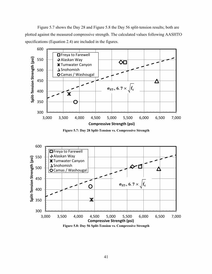
Figure 5.7 shows the Day 28 and Figure 5.8 the Day 56 split-tension results; both are
plotted against the measured compressive strength. The calculated values following AASHTO
specifications (Equation 2.4) are included in the figures.
Figure 5.7: Day 28 Split-Tension vs. Compressive Strength
Figure 5.8: Day 56 Split-Tension vs. Compressive Strength
300
350
400
450
500
550
600
3,000 3,500 4,000 4,500 5,000 5,500 6,000 6,500 7,000
Split
-Ten
sion
Str
engt
h (p
si)
Compressive Strength (psi)
Freya to FarewellAlaskan WayTumwater CanyonSnohomishCamas / Washougal
𝛔𝛔𝐒𝐒𝐒𝐒= 𝟔𝟔.𝟕𝟕 × 𝐟𝐟�̅�𝐜
300
350
400
450
500
550
600
3,000 3,500 4,000 4,500 5,000 5,500 6,000 6,500 7,000
Split
-Ten
sion
Str
engt
h (p
si)
Compressive Strength (psi)
Freya to FarewellAlaskan WayTumwater CanyonSnohomishCamas / Washougal
𝛔𝛔𝐒𝐒𝐒𝐒= 𝟔𝟔.𝟕𝟕 × 𝐟𝐟�̅�𝐜
41
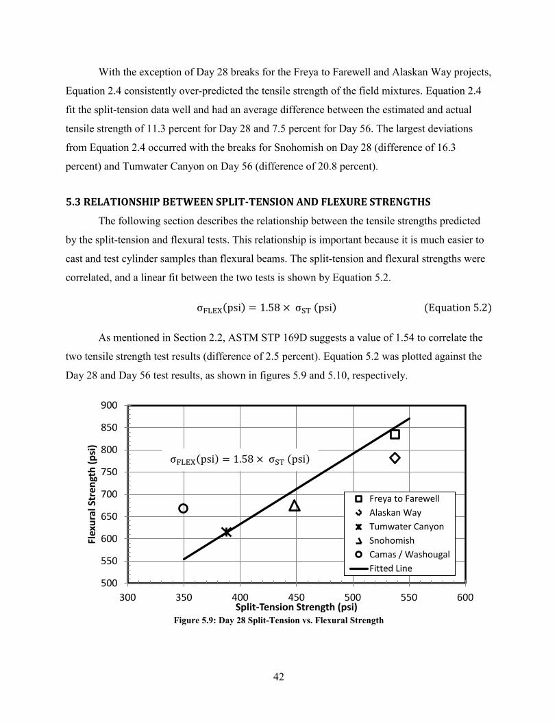
With the exception of Day 28 breaks for the Freya to Farewell and Alaskan Way projects,
Equation 2.4 consistently over-predicted the tensile strength of the field mixtures. Equation 2.4
fit the split-tension data well and had an average difference between the estimated and actual
tensile strength of 11.3 percent for Day 28 and 7.5 percent for Day 56. The largest deviations
from Equation 2.4 occurred with the breaks for Snohomish on Day 28 (difference of 16.3
percent) and Tumwater Canyon on Day 56 (difference of 20.8 percent).
5.3 RELATIONSHIP BETWEEN SPLIT-TENSION AND FLEXURE STRENGTHS
The following section describes the relationship between the tensile strengths predicted
by the split-tension and flexural tests. This relationship is important because it is much easier to
cast and test cylinder samples than flexural beams. The split-tension and flexural strengths were
correlated, and a linear fit between the two tests is shown by Equation 5.2.
σFLEX(psi) = 1.58 × σST (psi) (Equation 5.2)
As mentioned in Section 2.2, ASTM STP 169D suggests a value of 1.54 to correlate the
two tensile strength test results (difference of 2.5 percent). Equation 5.2 was plotted against the
Day 28 and Day 56 test results, as shown in figures 5.9 and 5.10, respectively.
Figure 5.9: Day 28 Split-Tension vs. Flexural Strength
500
550
600
650
700
750
800
850
900
300 350 400 450 500 550 600
Flex
ural
Str
engt
h (p
si)
Split-Tension Strength (psi)
Freya to FarewellAlaskan WayTumwater CanyonSnohomishCamas / WashougalFitted Line
σFLEX(psi) = 1.58 × σST (psi)
42

Figure 5.10: Day 56 Split Tension vs. Flexural Strength
Equation 5.2 fit the data set well, with the exception of the Day 28 break for
Camas/Washougal and Day 56 Snohomish break. Including all data points, the percentage error
in the predicted values from Equation 5.2 was an average of 7.6 percent for all of the mixtures.
The correlation coefficient was 7.2 percent for Day 28 and 8.0 percent for Day 56.
5.4 SUMMARY OF TENSILE STRENGTH RESULTS
The variation in flexural strengths among test specimens was small, with an average
variation of only 4 percent. The flexural strength increased a little between Day 28 and Day 56,
as expected. AASHTO code specifications for normal-weight concrete (Equation 2.2) under-
predicted the field sample strengths (figures 5.2 and 5.3). Equation 2.3, which is for high-
strength concrete, over-predicted the field sample strengths but had a smaller percentage
difference than Equation 2.2 (figures 5.2 and 5.3). The optimized Equation 5.1 fit the mean
flexural strength of the field mixtures and had a lower percentage difference than either
Equations 2.2 or 2.3 (figures 5.4 and 5.5).
The split-tension results showed large variation among samples. That variability in tensile
strength among samples had an average difference of 8 percent. Because of that large variation,
500
550
600
650
700
750
800
850
900
300 350 400 450 500 550 600
Flex
ural
Str
engt
h (p
si)
Split-Tension Strength (psi)
Freya to FarewellAlaskan WayTumwater CanyonSnohomishCamas / WashougalFitted Line
σFLEX(psi) = 1.58 × σST (psi)
43

it was not possible to measure a consistent trend in strength over time for the field mixtures. The
ACI specifications for estimating split-tensile strength (Equation 2.4) matched the field samples
within a 10 percent error (figures 5.7 and 5.8).
The measured split-tension and flexural strengths of the field concrete mixtures were fit
well by Equation 5.2 (figures 5.9 and 5.10). The correlation between the split-tension and
flexural strength tests found in the laboratory data was similar to the value suggested by
Equation 2.6 (difference of 2.5 percent). Because of the variability of the split-tension results,
further testing is required if the modulus of rupture is to be accurately predicted from the split-
tension strength tests.
44

Chapter 6: Elastic Modulus
This chapter discusses the results from the elastic modulus tests that were performed in
this study. The influences of the water-cementitious ratio, paste content, and coarse aggregate on
elastic modulus were evaluated.
Section 6.1 documents the data for a single aggregate source to illustrate the process used
to analyze the data. Section 6.2 summarizes and documents the data for the remaining aggregate
sources. The field mixture data are covered in Section 6.3. The details of the elastic modulus
tests are located in Appendix B.
6.1 LABORATORY DATA FOR DUPONT (3/4-IN.) AGGREGATE SOURCE
This section discusses the results from the elastic modulus tests performed on the DuPont
(3/4-in.) mixtures and the method of analyzing the data.
6.1.1 Measured Elastic Modulus
Elastic modulus tests were performed on two 6-in. x 12–in. cylinders for the laboratory
and field samples at days 7, 14, 28 and 56. The results of the elastic modulus tests on the four
DuPont (3/4-in.) mixtures are reported in Table 6.1, along with key mixture proportions.
Table 6.1: Measured Elastic Moduli: DuPont (3/4-in.) Mixtures
Mixture Paste
Content (%)
Water-Cementitious Ratio
Day 7 (ksi)
Day 14
(ksi)
Day 28
(ksi)
Day 56
(ksi) High Paste 30.5 0.38 4,460 4,900 5,160 5,260 Low Paste 24.0 0.38 3,910 4,280 4,560 4,610
High Strength 27.0 0.30 4,550 4,650 5,090 5,530 Low Strength 27.0 0.49 3,810 4,050 4,240 NA*
*The data for Day 56 for low-strength mixture were omitted from the data set because the strain gauge was not properly attached to the cylinders.
The elastic moduli for the Day 28 results ranged from 4,240 to 5,160 ksi, with an average
of 4,750 ksi. Figure 6.1 plots these data against the water-cementitious ratio for each mixture.
The figure also includes a fitted line of the form of Equation 6.1.
45
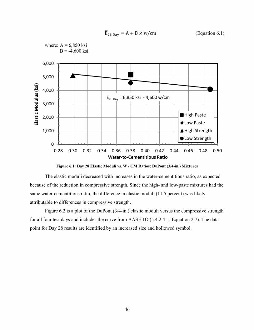
E�28 Day = A + B × w/cm (Equation 6.1) where: A = 6,850 ksi B = -4,600 ksi
Figure 6.1: Day 28 Elastic Moduli vs. W / CM Ratios: DuPont (3/4-in.) Mixtures
The elastic moduli decreased with increases in the water-cementitious ratio, as expected
because of the reduction in compressive strength. Since the high- and low-paste mixtures had the
same water-cementitious ratio, the difference in elastic moduli (11.5 percent) was likely
attributable to differences in compressive strength.
Figure 6.2 is a plot of the DuPont (3/4-in.) elastic moduli versus the compressive strength
for all four test days and includes the curve from AASHTO (5.4.2.4-1, Equation 2.7). The data
point for Day 28 results are identified by an increased size and hollowed symbol.
0
1,000
2,000
3,000
4,000
5,000
6,000
0.28 0.30 0.32 0.34 0.36 0.38 0.40 0.42 0.44 0.46 0.48 0.50
Elas
tic M
odul
us (k
si)
Water-to-Cementitious Ratio
High PasteLow PasteHigh StrengthLow Strength
E28 Day = 6,850 ksi - 4,600 w/cm
46

Figure 6.2: Elastic Moduli vs. Compressive Strengths: DuPont (3/4-in.) Mixtures
The elastic modulus for the DuPont (3/4-in.) aggregate exceeded by 14.6 percent, on
average, the calculated values for the AASHTO relationship (Equation 2.7). The measured
elastic moduli were normalized by dividing by the estimated elastic moduli from Equation 2.7 to
evaluate the accuracy of this equation. The resulting normalized elastic moduli ratios for the
DuPont (3/4-in.) mixtures are listed in Table 6.2.
Table 6.2: Measured to Calculated Elastic Moduli Ratio: DuPont (3/4-in.) Mixture
Day 7 Day 14 Day 28 Day 56 Average
High Paste 1.07 1.22* 1.12 1.10 1.13 Low Paste 1.18 1.23 1.21 1.18 1.20
High Strength 1.12 1.08 1.09 1.13 1.11 Low Strength 1.25 1.25 1.21 NA 1.24
Average 1.16 1.20 1.16 1.14 St. Deviation 0.08 0.08 0.06 0.04
Coef. of Variation 6.8% 6.5% 5.5% 3.4% *Day 14 compressive strength was low for DuPont (3/4-in.) High-Paste
2,500
3,000
3,500
4,000
4,500
5,000
5,500
6,000
2,500 3,000 3,500 4,000 4,500 5,000 5,500 6,000 6,500 7,000 7,500 8,000
Elas
tic M
odul
us (k
si)
Compressive Strength (psi)
High PasteLow PasteHigh StrengthLow StrengthAASHTO Curve
𝐸𝑐 = 33,000𝐾1𝑤𝑐1.5�𝑓�̅�
47
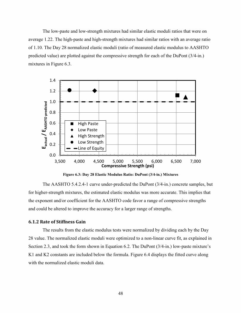
The low-paste and low-strength mixtures had similar elastic moduli ratios that were on
average 1.22. The high-paste and high-strength mixtures had similar ratios with an average ratio
of 1.10. The Day 28 normalized elastic moduli (ratio of measured elastic modulus to AASHTO
predicted value) are plotted against the compressive strength for each of the DuPont (3/4-in.)
mixtures in Figure 6.3.
Figure 6.3: Day 28 Elastic Modulus Ratio: DuPont (3/4-in.) Mixtures
The AASHTO 5.4.2.4-1 curve under-predicted the DuPont (3/4-in.) concrete samples, but
for higher-strength mixtures, the estimated elastic modulus was more accurate. This implies that
the exponent and/or coefficient for the AASHTO code favor a range of compressive strengths
and could be altered to improve the accuracy for a larger range of strengths.
6.1.2 Rate of Stiffness Gain
The results from the elastic modulus tests were normalized by dividing each by the Day
28 value. The normalized elastic moduli were optimized to a non-linear curve fit, as explained in
Section 2.3, and took the form shown in Equation 6.2. The DuPont (3/4-in.) low-paste mixture’s
K1 and K2 constants are included below the formula. Figure 6.4 displays the fitted curve along
with the normalized elastic moduli data.
0.0
0.2
0.4
0.6
0.8
1.0
1.2
1.4
3,500 4,000 4,500 5,000 5,500 6,000 6,500 7,000
E act
ual /
EAA
SHTO
pre
dict
ed
Compressive Strength (psi)
High PasteLow PasteHigh StrengthLow StrengthLine of Equity
48
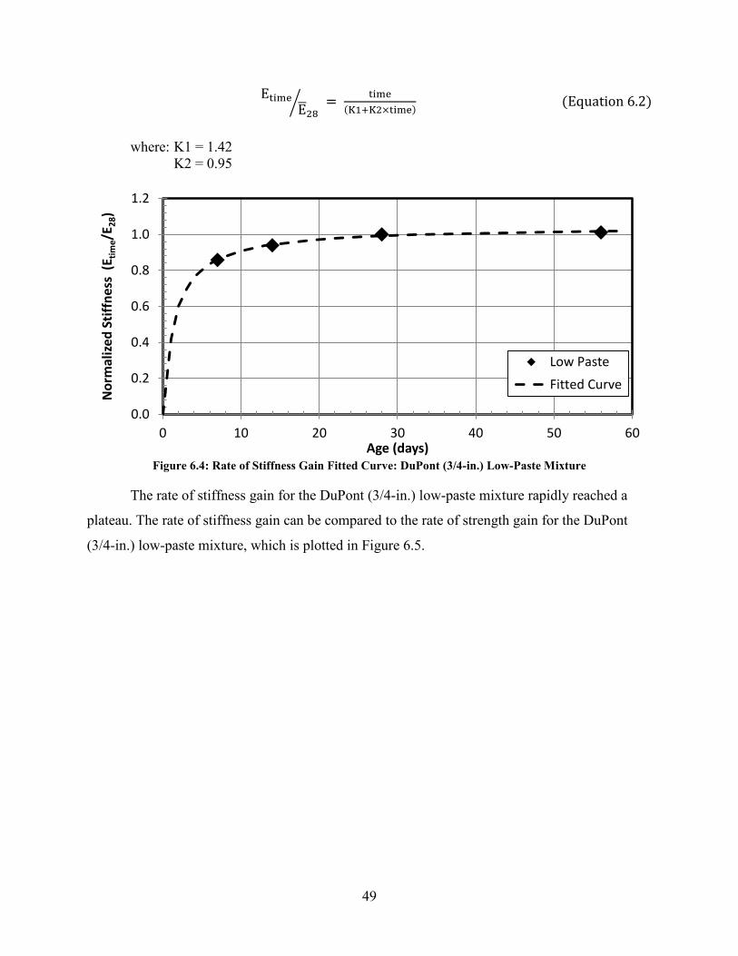
EtimeE�28� = time
(K1+K2×time) (Equation 6.2)
where: K1 = 1.42 K2 = 0.95
Figure 6.4: Rate of Stiffness Gain Fitted Curve: DuPont (3/4-in.) Low-Paste Mixture
The rate of stiffness gain for the DuPont (3/4-in.) low-paste mixture rapidly reached a
plateau. The rate of stiffness gain can be compared to the rate of strength gain for the DuPont
(3/4-in.) low-paste mixture, which is plotted in Figure 6.5.
0.0
0.2
0.4
0.6
0.8
1.0
1.2
0 10 20 30 40 50 60
Nor
mal
ized
Stiff
ness
(E t
ime/
E 28)
Age (days)
Low PasteFitted Curve
49
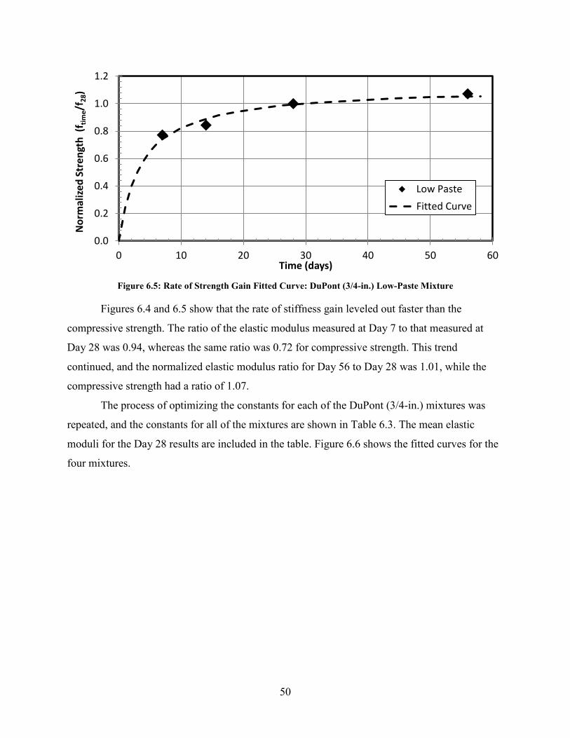
Figure 6.5: Rate of Strength Gain Fitted Curve: DuPont (3/4-in.) Low-Paste Mixture
Figures 6.4 and 6.5 show that the rate of stiffness gain leveled out faster than the
compressive strength. The ratio of the elastic modulus measured at Day 7 to that measured at
Day 28 was 0.94, whereas the same ratio was 0.72 for compressive strength. This trend
continued, and the normalized elastic modulus ratio for Day 56 to Day 28 was 1.01, while the
compressive strength had a ratio of 1.07.
The process of optimizing the constants for each of the DuPont (3/4-in.) mixtures was
repeated, and the constants for all of the mixtures are shown in Table 6.3. The mean elastic
moduli for the Day 28 results are included in the table. Figure 6.6 shows the fitted curves for the
four mixtures.
0.0
0.2
0.4
0.6
0.8
1.0
1.2
0 10 20 30 40 50 60
Nor
mal
ized
Stre
ngth
(f ti
me/
f 28)
Time (days)
Low PasteFitted Curve
50
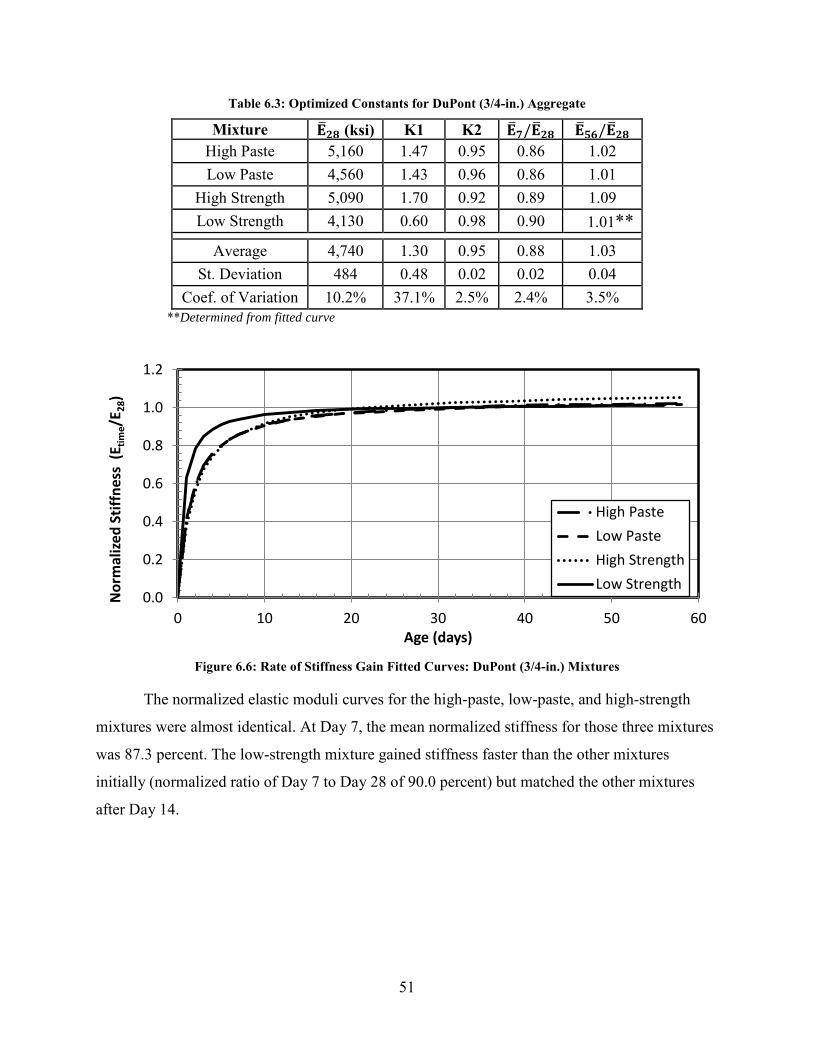
Table 6.3: Optimized Constants for DuPont (3/4-in.) Aggregate
Mixture 𝐄�𝟐𝟖 (ksi) K1 K2 𝐄�𝟕𝟕/𝐄�𝟐𝟖 𝐄�𝟓𝟔𝟔/𝐄�𝟐𝟖 High Paste 5,160 1.47 0.95 0.86 1.02 Low Paste 4,560 1.43 0.96 0.86 1.01
High Strength 5,090 1.70 0.92 0.89 1.09 Low Strength 4,130 0.60 0.98 0.90 1.01**
Average 4,740 1.30 0.95 0.88 1.03 St. Deviation 484 0.48 0.02 0.02 0.04
Coef. of Variation 10.2% 37.1% 2.5% 2.4% 3.5% **Determined from fitted curve
Figure 6.6: Rate of Stiffness Gain Fitted Curves: DuPont (3/4-in.) Mixtures
The normalized elastic moduli curves for the high-paste, low-paste, and high-strength
mixtures were almost identical. At Day 7, the mean normalized stiffness for those three mixtures
was 87.3 percent. The low-strength mixture gained stiffness faster than the other mixtures
initially (normalized ratio of Day 7 to Day 28 of 90.0 percent) but matched the other mixtures
after Day 14.
0.0
0.2
0.4
0.6
0.8
1.0
1.2
0 10 20 30 40 50 60
Nor
mal
ized
Stiff
ness
(E t
ime/
E 28)
Age (days)
High PasteLow PasteHigh StrengthLow Strength
51
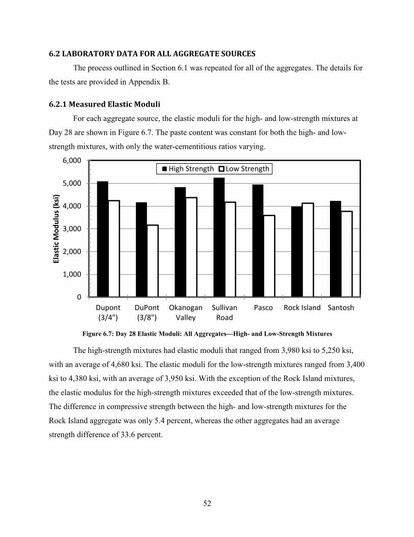
6.2 LABORATORY DATA FOR ALL AGGREGATE SOURCES
The process outlined in Section 6.1 was repeated for all of the aggregates. The details for
the tests are provided in Appendix B.
6.2.1 Measured Elastic Moduli
For each aggregate source, the elastic moduli for the high- and low-strength mixtures at
Day 28 are shown in Figure 6.7. The paste content was constant for both the high- and low-
strength mixtures, with only the water-cementitious ratios varying.
Figure 6.7: Day 28 Elastic Moduli: All Aggregates—High- and Low-Strength Mixtures
The high-strength mixtures had elastic moduli that ranged from 3,980 ksi to 5,250 ksi,
with an average of 4,680 ksi. The elastic moduli for the low-strength mixtures ranged from 3,400
ksi to 4,380 ksi, with an average of 3,950 ksi. With the exception of the Rock Island mixtures,
the elastic modulus for the high-strength mixtures exceeded that of the low-strength mixtures.
The difference in compressive strength between the high- and low-strength mixtures for the
Rock Island aggregate was only 5.4 percent, whereas the other aggregates had an average
strength difference of 33.6 percent.
0
1,000
2,000
3,000
4,000
5,000
6,000
Dupont(3/4")
DuPont(3/8")
OkanoganValley
SullivanRoad
Pasco Rock Island Santosh
Elas
tic M
odul
us (k
si)
High Strength Low Strength
52

The Day 28 elastic moduli were analyzed against the water-cementitious ratio and fit to
the line for Equation 6.1 for each aggregate source. Figure 6.8 shows the resulting linear fits for
the seven aggregate sources. The individual plots for the elastic moduli versus water-
cementitious ratios can be seen in Appendix B for the various aggregate sources. There was little
change in elastic moduli as a function of water-cementitious ratio for Rock Island mixtures,
which can be seen in Figure B.5.
Figure 6.8: Day 28 Elastic Modulus vs. Water-Cementitious Ratio: All Aggregates
Excluding the Rock Island aggregate, raising the water-cementitious ratio decreased the
elastic modulus for the aggregates. An increase of 0.1 in the water-cementitious ratio reduced the
elastic moduli in a range of 205 ksi to 735 ksi, with an average decrease of 470 ksi. The average
change in compressive strength per change of 0.1 water-cementitious ratios was 1,200 psi. This
suggests that for the range of water-cementitious ratios between 0.30 and 0.49, the elastic
modulus increases at approximately 40 percent of the rate of the compressive strength. This
supports the finding that elastic modulus increases more slowly than the strength, and an
exponent of less than 1.0 should be used to correlate the strength to the elastic modulus.
0
1,000
2,000
3,000
4,000
5,000
6,000
0.28 0.30 0.32 0.34 0.36 0.38 0.40 0.42 0.44 0.46 0.48 0.50 0.52
Elas
tic M
odul
us (k
si)
Water-to-Cement Ratio
Dupont (3/4")DuPont (3/8")Okanogan ValleySullivan RoadPascoRock IslandSantosh
53
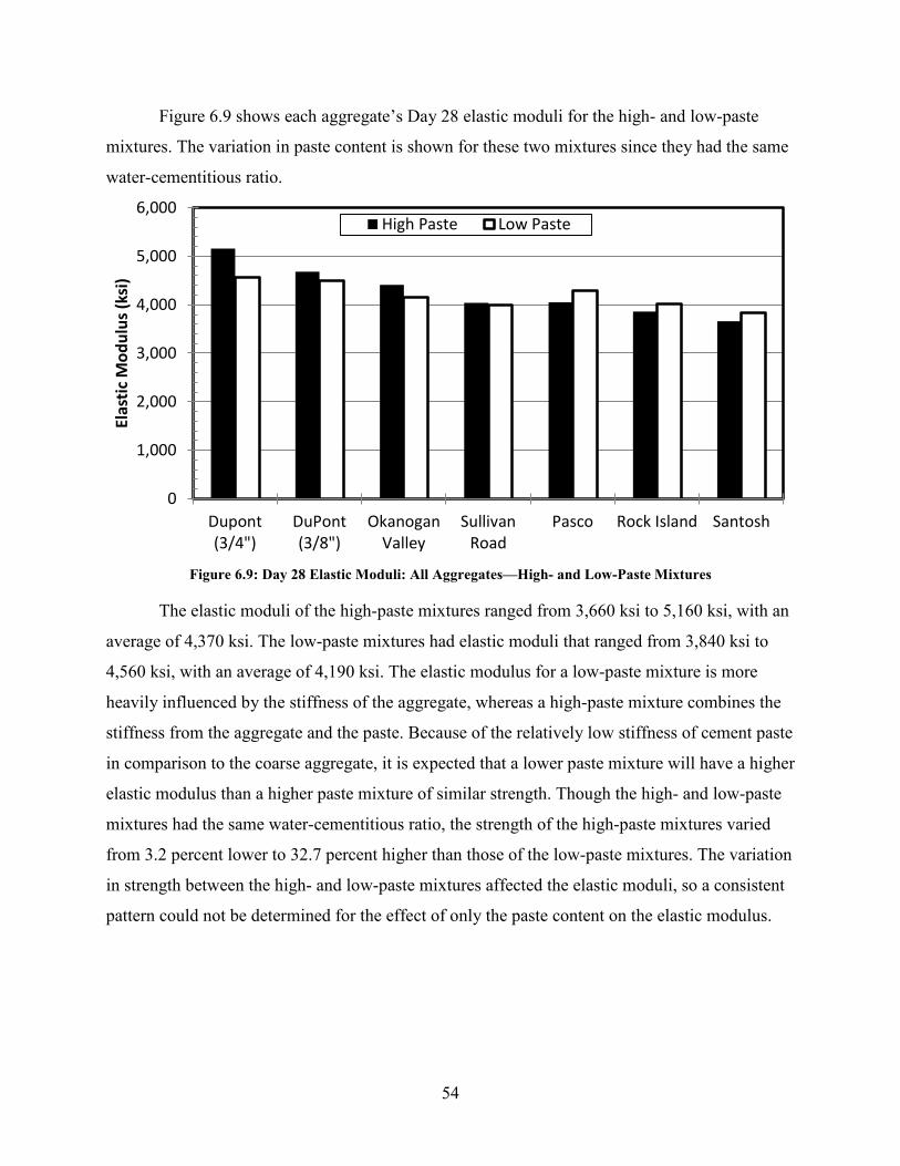
Figure 6.9 shows each aggregate’s Day 28 elastic moduli for the high- and low-paste
mixtures. The variation in paste content is shown for these two mixtures since they had the same
water-cementitious ratio.
Figure 6.9: Day 28 Elastic Moduli: All Aggregates—High- and Low-Paste Mixtures
The elastic moduli of the high-paste mixtures ranged from 3,660 ksi to 5,160 ksi, with an
average of 4,370 ksi. The low-paste mixtures had elastic moduli that ranged from 3,840 ksi to
4,560 ksi, with an average of 4,190 ksi. The elastic modulus for a low-paste mixture is more
heavily influenced by the stiffness of the aggregate, whereas a high-paste mixture combines the
stiffness from the aggregate and the paste. Because of the relatively low stiffness of cement paste
in comparison to the coarse aggregate, it is expected that a lower paste mixture will have a higher
elastic modulus than a higher paste mixture of similar strength. Though the high- and low-paste
mixtures had the same water-cementitious ratio, the strength of the high-paste mixtures varied
from 3.2 percent lower to 32.7 percent higher than those of the low-paste mixtures. The variation
in strength between the high- and low-paste mixtures affected the elastic moduli, so a consistent
pattern could not be determined for the effect of only the paste content on the elastic modulus.
0
1,000
2,000
3,000
4,000
5,000
6,000
Dupont(3/4")
DuPont(3/8")
OkanoganValley
SullivanRoad
Pasco Rock Island Santosh
Elas
tic M
odul
us (k
si)
High Paste Low Paste
54
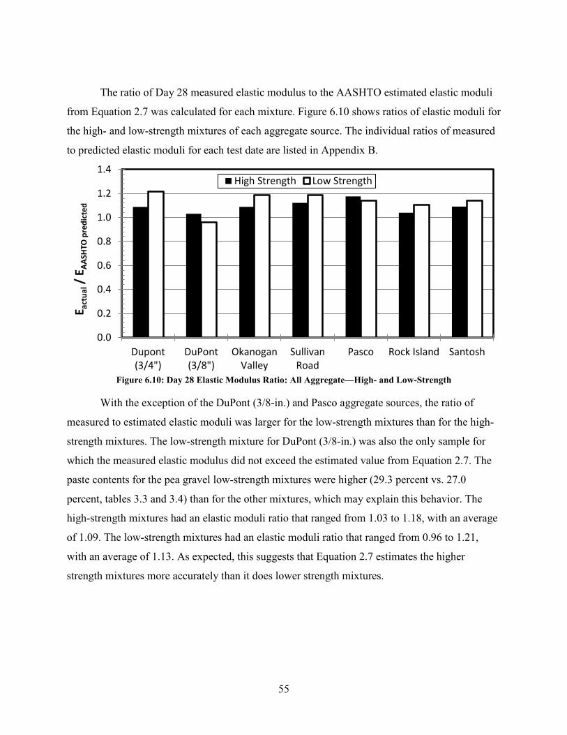
The ratio of Day 28 measured elastic modulus to the AASHTO estimated elastic moduli
from Equation 2.7 was calculated for each mixture. Figure 6.10 shows ratios of elastic moduli for
the high- and low-strength mixtures of each aggregate source. The individual ratios of measured
to predicted elastic moduli for each test date are listed in Appendix B.
Figure 6.10: Day 28 Elastic Modulus Ratio: All Aggregate—High- and Low-Strength
With the exception of the DuPont (3/8-in.) and Pasco aggregate sources, the ratio of
measured to estimated elastic moduli was larger for the low-strength mixtures than for the high-
strength mixtures. The low-strength mixture for DuPont (3/8-in.) was also the only sample for
which the measured elastic modulus did not exceed the estimated value from Equation 2.7. The
paste contents for the pea gravel low-strength mixtures were higher (29.3 percent vs. 27.0
percent, tables 3.3 and 3.4) than for the other mixtures, which may explain this behavior. The
high-strength mixtures had an elastic moduli ratio that ranged from 1.03 to 1.18, with an average
of 1.09. The low-strength mixtures had an elastic moduli ratio that ranged from 0.96 to 1.21,
with an average of 1.13. As expected, this suggests that Equation 2.7 estimates the higher
strength mixtures more accurately than it does lower strength mixtures.
0.0
0.2
0.4
0.6
0.8
1.0
1.2
1.4
Dupont(3/4")
DuPont(3/8")
OkanoganValley
SullivanRoad
Pasco Rock Island Santosh
E act
ual /
EAA
SHTO
pre
dict
ed
High Strength Low Strength
55

Figure 6.11 shows the ratio of measured to AASHTO estimated elastic moduli for the
high- and low-paste mixtures.
Figure 6.11: Day 28 Elastic Modulus Ratio: All Aggregate—High- and Low-Paste
Excluding the DuPont (3/8-in.) and Sullivan Road aggregate, the ratio between the
measured and estimated elastic modulus was larger for the low-paste mixtures than for the high-
paste mixtures. The high-paste mixtures had a ratio that ranged from 1.03 to 1.14, with an
average of 1.08. The low-paste mixtures had a range of 1.01 to 1.21 and an average ratio of 1.12.
This follows the same suggestion that the AASHTO specifications for estimating the elastic
modulus based on compressive strength (Equation 2.7) are more accurate for higher strength
concrete mixtures.
6.2.2 Rate of Stiffness Gain
The measured elastic moduli for each mixture were normalized by dividing the data by
the respective Day 28 elastic moduli. Figure 6.12 shows the normalized elastic moduli for the
high- and low-strength mixtures as a ratio of Day 7 to Day 28 values for each of the aggregates.
Each mixture’s normalized elastic modulus data were fit to Equation 6.2; the optimized K1 and
K2 coefficients and fitted curves can be seen in Appendix B.
0.0
0.2
0.4
0.6
0.8
1.0
1.2
1.4
Dupont(3/4")
DuPont(3/8")
OkanoganValley
SullivanRoad
Pasco Rock Island Santosh
E act
ual /
EAA
SHTO
pre
dict
ed
High Paste Low Paste
56

Figure 6.12: Day 28 Rate of Stiffness Gain: All Aggregates-High- and Low-Strength
The ratio of Day 7 to Day 28 stiffness was nearly identical for the high-strength and low-
strength mixtures. The normalized stiffness ratio for the Day 7 to Day 28 elastic moduli of the
high-strength mixture ranged from 0.89 to 0.92, with an average ratio of 0.91. The low-strength
mixtures had a ratio that ranged from 0.84 to 0.92, with an average of 0.89. The percentage
difference between the high and low strength mixtures ranged from 0.6 percent to 5.8 percent,
with a mean of 2.7 percent. The variation in water-cementitious ratio, aggregate type, and cement
content did not have a large effect on the early rate of stiffness gain for mixtures with constant
paste content.
Figure 6.13 shows the normalized Day 7 to Day 28 ratio of the elastic moduli for the
high- and low-paste mixtures.
0.00.10.20.30.40.50.60.70.80.91.01.1
Dupont(3/4")
DuPont(3/8")
OkanoganValley
SullivanRoad
Pasco Rock Island Santosh
Nor
mal
ized
Stiff
ness
(E7/
E 28)
High Strength Low Strength
57

Figure 6.13: Day 28 Rate of Stiffness Gain: All Aggregates-High- and Low-Paste
The normalized Day 7 to 28 rate of stiffness gain for the high-paste mixtures ranged from
0.80 to 0.96, with an average rate of 0.89. The low-paste mixtures had a normalized stiffness
gain that ranged from 0.84 to 1.01, with an average of 0.91. The percentage difference between
the high- and low-paste mixtures ranged from 0.0 percent to 14.3 percent, with an average of 6.7
percent. There was no consistent pattern across the different aggregate sources, so the effect of
the paste content on the rate of stiffness gain was not determined.
6.3 DATA FOR FIELD SAMPLES
This section discusses the results from the elastic modulus tests performed on the field
samples for each of the five WSDOT projects.
6.3.1 Measured Elastic Moduli
The mixture proportions and elastic moduli for each testing day are shown for the five
WSDOT projects in Table 6.4.
0.00.10.20.30.40.50.60.70.80.91.01.1
Dupont(3/4")
DuPont(3/8")
OkanoganValley
SullivanRoad
Pasco Rock Island Santosh
Nor
mal
ized
Stiff
ness
(E7/
E 28)
High Paste Low Paste
58
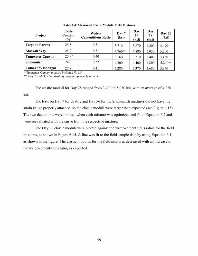
Table 6.4: Measured Elastic Moduli: Field Mixtures
Project Paste
Content (%)
Water-Cementitious Ratio
Day 7 (ksi)
Day 14
(ksi)
Day 28
(ksi)
Day 56 (ksi)
Freya to Farewell 25.5 0.31 3,710 3,870 4,200 4,490 Alaskan Way 25.2 0.31 4,760** 4,880 5,030 5,200 Tumwater Canyon 25.9* 0.40 3,160 3,210 3,400 3,450 Snohomish 24.6 0.32 4,200 4,460 4,800 5,240** Camas / Washougal 27.8 0.41 3,280 3,370 3,680 3,870
* Tumwater Canyon mixture included fly ash ** Day 7 and Day 56: strain gauges not properly attached
The elastic moduli for Day 28 ranged from 3,400 to 5,030 ksi, with an average of 4,220
ksi.
The tests on Day 7 for Seattle and Day 56 for the Snohomish mixtures did not have the
strain gauge properly attached, so the elastic moduli were larger than expected (see Figure 6.15).
The two data points were omitted when each mixture was optimized and fit to Equation 6.2 and
were reevaluated with the curve from the respective mixture.
The Day 28 elastic moduli were plotted against the water-cementitious ratios for the field
mixtures, as shown in Figure 6.14. A line was fit to the field sample data by using Equation 6.1,
as shown in the figure. The elastic modulus for the field mixtures decreased with an increase in
the water-cementitious ratio, as expected.
59

Figure 6.14: Day 28 Elastic Modulus vs. Water-Cementitious Ratio: Field Mixtures
Figure 6.15 is a plot of the elastic moduli versus compressive strengths for each of the
field mixtures on all four of the testing days. The AASHTO 5.4.2.4-1 equation is included in the
figure (Equation 2.7). Since the AASHTO specifications use the design compressive strength,
the data point for the Day 28 test results of each field mixture are indicated by a solid fill and
increasing the size.
E28 Day = 8,420 -12,000 x w/cm
0
1,000
2,000
3,000
4,000
5,000
6,000
7,000
8,000
0.28 0.30 0.32 0.34 0.36 0.38 0.40 0.42 0.44
Elas
tic M
odul
us (k
si)
Water-Cementitious Ratio
Freya to FarewellAlaskan WayTumwater CanyonSnohomishCamas / Washougal
60
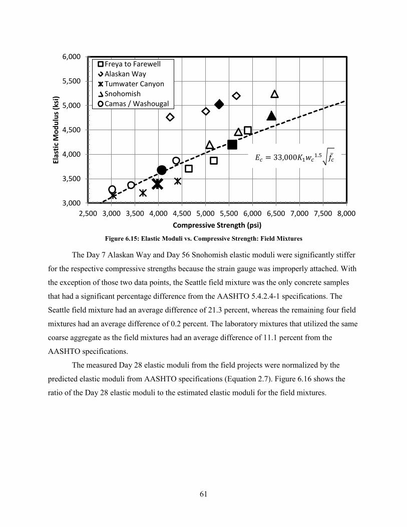
Figure 6.15: Elastic Moduli vs. Compressive Strength: Field Mixtures
The Day 7 Alaskan Way and Day 56 Snohomish elastic moduli were significantly stiffer
for the respective compressive strengths because the strain gauge was improperly attached. With
the exception of those two data points, the Seattle field mixture was the only concrete samples
that had a significant percentage difference from the AASHTO 5.4.2.4-1 specifications. The
Seattle field mixture had an average difference of 21.3 percent, whereas the remaining four field
mixtures had an average difference of 0.2 percent. The laboratory mixtures that utilized the same
coarse aggregate as the field mixtures had an average difference of 11.1 percent from the
AASHTO specifications.
The measured Day 28 elastic moduli from the field projects were normalized by the
predicted elastic moduli from AASHTO specifications (Equation 2.7). Figure 6.16 shows the
ratio of the Day 28 elastic moduli to the estimated elastic moduli for the field mixtures.
3,000
3,500
4,000
4,500
5,000
5,500
6,000
2,500 3,000 3,500 4,000 4,500 5,000 5,500 6,000 6,500 7,000 7,500 8,000
Elas
tic M
odul
us (k
si)
Compressive Strength (psi)
Freya to FarewellAlaskan WayTumwater CanyonSnohomishCamas / Washougal
𝐸𝑐 = 33,000𝐾1𝑤𝑐1.5�𝑓�̅�
61
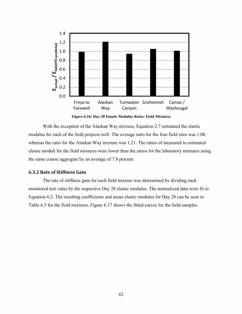
Figure 6.16: Day 28 Elastic Modulus Ratio: Field Mixtures
With the exception of the Alaskan Way mixture, Equation 2.7 estimated the elastic
modulus for each of the field projects well. The average ratio for the four field sites was 1.00,
whereas the ratio for the Alaskan Way mixture was 1.21. The ratios of measured to estimated
elastic moduli for the field mixtures were lower than the ratios for the laboratory mixtures using
the same coarse aggregate by an average of 7.8 percent.
6.3.2 Rate of Stiffness Gain
The rate of stiffness gain for each field mixture was determined by dividing each
monitored test value by the respective Day 28 elastic modulus. The normalized data were fit to
Equation 6.2. The resulting coefficients and mean elastic modulus for Day 28 can be seen in
Table 6.5 for the field mixtures. Figure 6.17 shows the fitted curves for the field samples.
0.0
0.2
0.4
0.6
0.8
1.0
1.2
1.4
Freya toFarewell
AlaskanWay
TumwaterCanyon
Snohomish Camas /Washougal
E act
ual /
EAA
SHTO
pre
dict
ed
62

Table 6.5: Optimized Constants for Field Samples
Project 𝐄�𝟐𝟖 (ksi) K1 K2 𝐄�𝟕𝟕/𝐄�𝟐𝟖 𝐄𝟓𝟔𝟔/𝐄�𝟐𝟖
Freya to Farewell 5,570 1.74 0.93 0.88 1.07 Alaskan Way 5,290 1.10 0.95 0.90** 1.03 Tumwater Canyon 3,980 0.93 0.98 0.91 1.01 Snohomish 6,400 1.38 0.96 0.87 1.02** Camas / Washougal 4,070 1.41 0.95 0.89 1.05
Average 5,060 1.27 0.95 0.90 1.05 St. Deviation 1,030 0.57 0.02 0.03 0.03 Coef. Of Variation 20.4% 23.9% 1.6% 1.4% 2.3%
** Determined from fitted curve
Figure 6.17: Rate of Stiffness Gain Fitted Curves: Field Mixtures
The rate of stiffness gain for the five field mixtures was very similar. After Day 7, the
normalized elastic moduli had less than a 3 percent coefficient of variation. Only the initial rate
of stiffness gain before Day 7 varied among field samples. This can be attributed to the
variations in compressive strength or cement content.
0.0
0.2
0.4
0.6
0.8
1.0
1.2
0 10 20 30 40 50 60
Nor
mal
ized
Stiff
ness
(Etim
e/E 2
8)
Age (days)
Freya to FarewellAlaskan WayTunwater CanyonSnohomishCamas / Washougal
63

The rate of stiffness gain for the ratio of Day 7 to Day 28 elastic moduli was plotted
against the water-cementitious ratio and the paste content of the field mixtures, as shown in
Figure 6.18 and Figure 6.19, respectively. As expected, the water-cementitious ratio and paste
content did little to affect the rate of stiffness gain for each of the different aggregate sources.
Figure 6.18: Rate of Stiffness Gain vs. Water-Cementitious Ratio: Field Mixtures
Figure 6.19: Rate of Stiffness Gain vs. Paste Content: Field Mixtures
E7/E28 = 0.89 + 0.04 x w/cm
0.00.10.20.30.40.50.60.70.80.91.0
0.28 0.30 0.32 0.34 0.36 0.38 0.40 0.42 0.44
Nor
mal
ized
Stiff
ness
(E7/
E 28)
Water-Cementitious Ratio
Freya to FarewellAlaskan WayTumwater CanyonSnohomishCamas / Washougal
E7/E28 = 0.90 + 0.0003 x Paste Content
0.00.10.20.30.40.50.60.70.80.91.0
22 24 26 28 30
Nor
mal
ized
Stiff
ness
(E7/
E 28)
Paste Content
Freya to FarewellAlaskan WayTumwater CanyonSnohomishCamas / Washougal
64
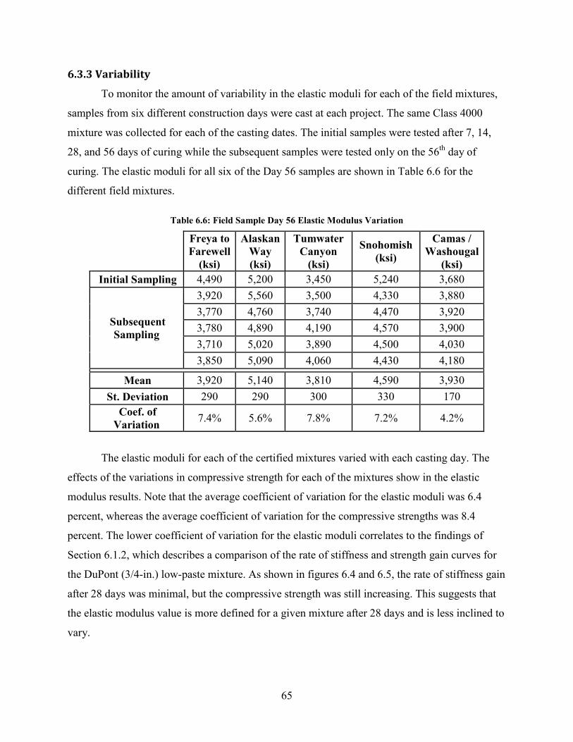
6.3.3 Variability
To monitor the amount of variability in the elastic moduli for each of the field mixtures,
samples from six different construction days were cast at each project. The same Class 4000
mixture was collected for each of the casting dates. The initial samples were tested after 7, 14,
28, and 56 days of curing while the subsequent samples were tested only on the 56th day of
curing. The elastic moduli for all six of the Day 56 samples are shown in Table 6.6 for the
different field mixtures.
Table 6.6: Field Sample Day 56 Elastic Modulus Variation
Freya to Farewell
(ksi)
Alaskan Way (ksi)
Tumwater Canyon
(ksi)
Snohomish (ksi)
Camas / Washougal
(ksi) Initial Sampling 4,490 5,200 3,450 5,240 3,680
Subsequent Sampling
3,920 5,560 3,500 4,330 3,880 3,770 4,760 3,740 4,470 3,920 3,780 4,890 4,190 4,570 3,900 3,710 5,020 3,890 4,500 4,030 3,850 5,090 4,060 4,430 4,180
Mean 3,920 5,140 3,810 4,590 3,930 St. Deviation 290 290 300 330 170
Coef. of Variation 7.4% 5.6% 7.8% 7.2% 4.2%
The elastic moduli for each of the certified mixtures varied with each casting day. The
effects of the variations in compressive strength for each of the mixtures show in the elastic
modulus results. Note that the average coefficient of variation for the elastic moduli was 6.4
percent, whereas the average coefficient of variation for the compressive strengths was 8.4
percent. The lower coefficient of variation for the elastic moduli correlates to the findings of
Section 6.1.2, which describes a comparison of the rate of stiffness and strength gain curves for
the DuPont (3/4-in.) low-paste mixture. As shown in figures 6.4 and 6.5, the rate of stiffness gain
after 28 days was minimal, but the compressive strength was still increasing. This suggests that
the elastic modulus value is more defined for a given mixture after 28 days and is less inclined to
vary.
65

6.3.4 Comparison of Laboratory and Field Data
Table 6.7 shows the average compressive strengths and elastic moduli of the Day 56
samples from the field sites. The elastic modulus predicted from the AASHTO specifications
(5.4.2.4-1, Equation 2.7) and the percentage difference between the measured and estimated
elastic modulus are included in the table.
Table 6.7: AASHTO Predicted Field Sample Elastic Moduli
Project Average Comp.
Strength (psi)
Average Elastic
Modulus (ksi)
Predicted Elastic Modulus
(ksi)
Percentage Difference
Freya to Farewell 5,280 3,920 4,180 6.2% Alaskan Way 5,830 5,140 4,390 14.6% Tumwater Canyon 4,830 3,810 4,000 4.8% Snohomish 5,270 4,590 4,140 9.8% Camas /
Washougal 4,410 3,930 3,790 3.6%
The difference in estimated and actual elastic moduli ranged from 3.6 percent to 14.6
percent, with an average difference of 7.8 percent. This suggests that the AASHTO
specifications (5.4.2.4-1, Equation 2.7) predict the elastic modulus well for a concrete mixture
without including parameters for the aggregate source, paste content, or water-to-cementitious
ratio. For the Tumwater Canyon and Freya to Farewell mixtures, AASHTO specifications over-
predicted the elastic modulus (predicted values were on average 5.5 percent larger). The Alaskan
Way, Snohomish, and Camas/Washougal projects had estimated elastic moduli that were under-
predicted (predicted values were on average 9.3 percent smaller).
An alternative formula was derived to account for the mixture proportions and
compressive strength in estimating the elastic modulus. Equation 6.3 shows the formatting and
optimized constants that were derived from the laboratory mixtures based on the Day 28 results.
66
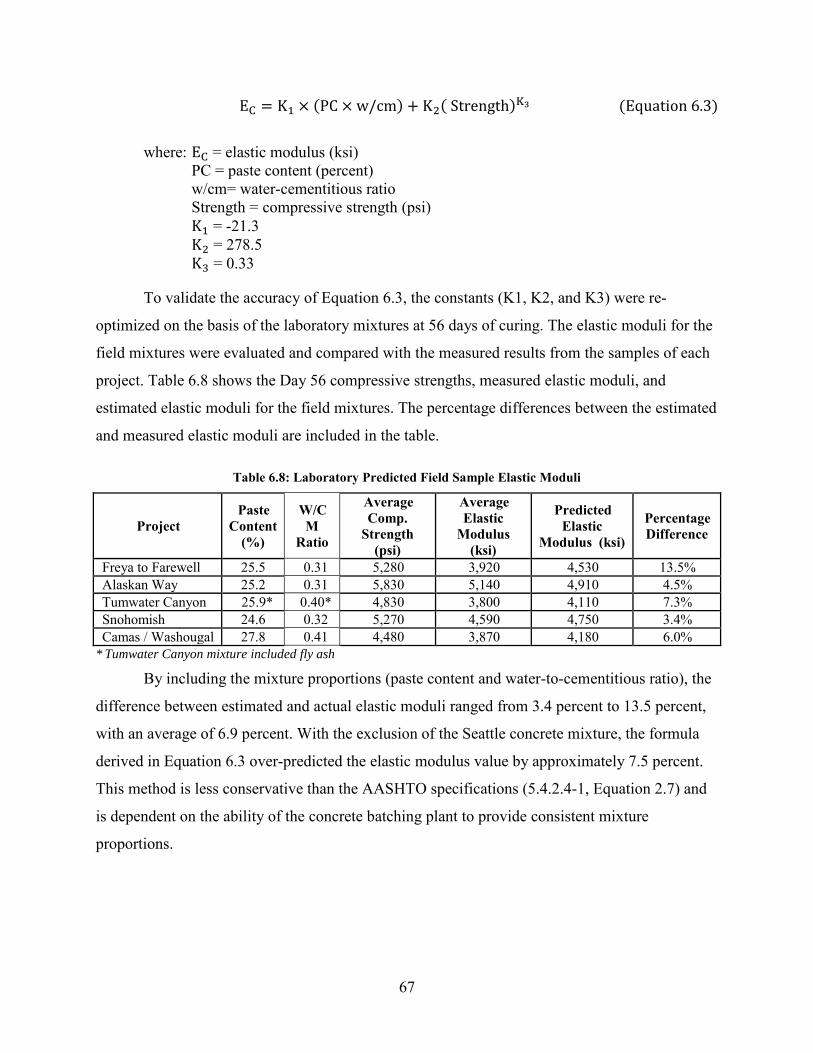
EC = K1 × (PC × w/cm) + K2( Strength)K3 (Equation 6.3)
where: EC = elastic modulus (ksi) PC = paste content (percent) w/cm= water-cementitious ratio Strength = compressive strength (psi)
K1 = -21.3 K2 = 278.5 K3 = 0.33
To validate the accuracy of Equation 6.3, the constants (K1, K2, and K3) were re-
optimized on the basis of the laboratory mixtures at 56 days of curing. The elastic moduli for the
field mixtures were evaluated and compared with the measured results from the samples of each
project. Table 6.8 shows the Day 56 compressive strengths, measured elastic moduli, and
estimated elastic moduli for the field mixtures. The percentage differences between the estimated
and measured elastic moduli are included in the table.
Table 6.8: Laboratory Predicted Field Sample Elastic Moduli
Project Paste
Content (%)
W/CM
Ratio
Average Comp.
Strength (psi)
Average Elastic
Modulus (ksi)
Predicted Elastic
Modulus (ksi)
Percentage Difference
Freya to Farewell 25.5 0.31 5,280 3,920 4,530 13.5% Alaskan Way 25.2 0.31 5,830 5,140 4,910 4.5% Tumwater Canyon 25.9* 0.40* 4,830 3,800 4,110 7.3% Snohomish 24.6 0.32 5,270 4,590 4,750 3.4% Camas / Washougal 27.8 0.41 4,480 3,870 4,180 6.0%
* Tumwater Canyon mixture included fly ash
By including the mixture proportions (paste content and water-to-cementitious ratio), the
difference between estimated and actual elastic moduli ranged from 3.4 percent to 13.5 percent,
with an average of 6.9 percent. With the exclusion of the Seattle concrete mixture, the formula
derived in Equation 6.3 over-predicted the elastic modulus value by approximately 7.5 percent.
This method is less conservative than the AASHTO specifications (5.4.2.4-1, Equation 2.7) and
is dependent on the ability of the concrete batching plant to provide consistent mixture
proportions.
67

6.4 ANALYSIS OF ELASTIC MODULUS RESULTS
The variations in the compressive strength and aggregate type significantly affected the
elastic modulus (figures 6.2 and 6.15). A reduction in the water-cementitious ratio increased the
compressive strength and elastic modulus (figures 4.6, 6.1, 6.8, and 6.14). The changes in
compressive strength and elastic modulus due to a change in water-cementitious ratio were not
similar. The effect of the paste content on the elastic modulus was not able to be determined
(Figure 6.9).
The rate of stiffness gain was not affected by the compressive strength or aggregate
source (figures 6.12 and 6.18). The paste content did not consistently affect the rate of stiffness
gain (figures 6.13 and 6.19).
AASHTO specifications (5.4.2.4-1, Equation 2.7) estimated the elastic moduli of the field
mixtures well but were less accurate for the laboratory mixtures (Table 6.2 and figures 6.10,
6.11, and 6.17). Equation 2.7 estimated the elastic modulus for higher strength mixtures more
accurately than for lower strength mixtures (Figure 6.3). By accounting for the effect of the paste
content on the elastic modulus in Equation 6.3, the percentage difference between the estimated
value and the measured elastic modulus was 6.9 percent (the AASHTO specifications had a
difference of 7.8 percent).
68

Chapter 7: Drying Shrinkage
The results of the drying shrinkage tests that were performed and monitored for a year’s
duration are discussed in this chapter. The effects of water-cementitious ratio, paste content,
compressive strength, and coarse aggregate on the drying shrinkage are analyzed in this chapter.
The results from a single aggregate source are presented in Section 7.1 to document the
procedure used to analyze the shrinkage data. A summary of all of the laboratory aggregate
sources is discussed in Section 7.2 and includes the trends that were identified. Section 7.3 gives
the shrinkage results from the field mixtures. The shrinkage that occurred over a year’s duration
is compared with the allowable strain for fatigue in Section 7.4. The details of the drying
shrinkage tests are provided in Appendix D.
7.1 LABORATORY DATA FOR DUPONT (3/4-IN.) AGGREGATE SOURCE
Three drying shrinkage samples were cast for each laboratory and field mixture to
perform the drying shrinkage tests. The three samples were submerged in a Calcium Hydroxide
saturated solution to moist-cure for 28 days. After this curing period, the samples were placed in
a temperature-controlled room to air dry for a year.
As explained in Section 2.4, the drying shrinkage strains were fit to a non-linear curve
which can be seen in Equation 7.1. The optimized constants (t50 and ϵ Ult.) for the DuPont (3/4-
in.) low-strength mixture were included to show typical values. The monitored shrinkage data
and fitted curve are plotted in Figure 7.1.
ϵ time = time(t50+time) × ϵ Ult. (Equation 7.1)
where: t50 = 25.5 days ϵ Ult. = 810 microstrain time = Drying duration (days)
69
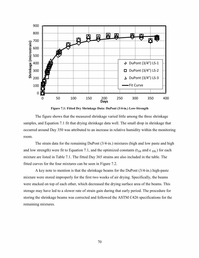
Figure 7.1: Fitted Dry Shrinkage Data: DuPont (3/4-in.) Low-Strength
The figure shows that the measured shrinkage varied little among the three shrinkage
samples, and Equation 7.1 fit that drying shrinkage data well. The small drop in shrinkage that
occurred around Day 350 was attributed to an increase in relative humidity within the monitoring
room.
The strain data for the remaining DuPont (3/4-in.) mixtures (high and low paste and high
and low strength) were fit to Equation 7.1, and the optimized constants (t50 and ϵ Ult.) for each
mixture are listed in Table 7.1. The fitted Day 365 strains are also included in the table. The
fitted curves for the four mixtures can be seen in Figure 7.2.
A key note to mention is that the shrinkage beams for the DuPont (3/4-in.) high-paste
mixture were stored improperly for the first two weeks of air drying. Specifically, the beams
were stacked on top of each other, which decreased the drying surface area of the beams. This
storage may have led to a slower rate of strain gain during that early period. The procedure for
storing the shrinkage beams was corrected and followed the ASTM C426 specifications for the
remaining mixtures.
0
100
200
300
400
500
600
700
800
900
0 50 100 150 200 250 300 350 400
Shrin
kage
(mic
rost
rain
)
Days
DuPont (3/4") LS-1
DuPont (3/4") LS-2
DuPont (3/4") LS-3
Fit Curve
70
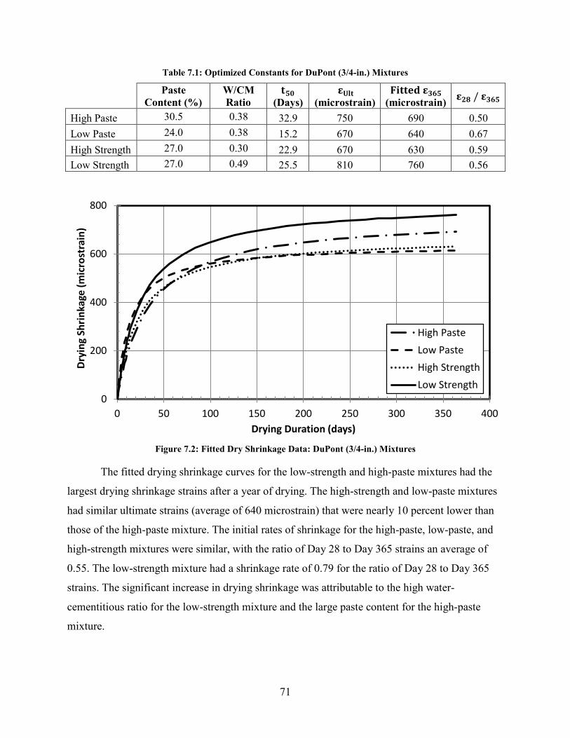
Table 7.1: Optimized Constants for DuPont (3/4-in.) Mixtures
Paste Content (%)
W/CM Ratio
𝐭𝟓𝟎 (Days)
𝛆𝐔𝐥𝐭 (microstrain)
𝐅𝐢𝐭𝐭𝐞𝐝 𝛆𝟑𝟔𝟔𝟓 (microstrain) 𝛆𝟐𝟖 / 𝛆𝟑𝟔𝟔𝟓
High Paste 30.5 0.38 32.9 750 690 0.50 Low Paste 24.0 0.38 15.2 670 640 0.67 High Strength 27.0 0.30 22.9 670 630 0.59 Low Strength 27.0 0.49 25.5 810 760 0.56
Figure 7.2: Fitted Dry Shrinkage Data: DuPont (3/4-in.) Mixtures
The fitted drying shrinkage curves for the low-strength and high-paste mixtures had the
largest drying shrinkage strains after a year of drying. The high-strength and low-paste mixtures
had similar ultimate strains (average of 640 microstrain) that were nearly 10 percent lower than
those of the high-paste mixture. The initial rates of shrinkage for the high-paste, low-paste, and
high-strength mixtures were similar, with the ratio of Day 28 to Day 365 strains an average of
0.55. The low-strength mixture had a shrinkage rate of 0.79 for the ratio of Day 28 to Day 365
strains. The significant increase in drying shrinkage was attributable to the high water-
cementitious ratio for the low-strength mixture and the large paste content for the high-paste
mixture.
0
200
400
600
800
0 50 100 150 200 250 300 350 400
Dryi
ng S
hrin
kage
(mic
rost
rain
)
Drying Duration (days)
High PasteLow PasteHigh StrengthLow Strength
71

The creep and drying shrinkage samples were stored in the same temperature-controlled
room as the drying shrinkage beams. Since the drying shrinkage cylinders and beams were
exposed to the same conditions for most of the year, the two shrinkage types of samples could be
compared. There were two differences between the shrinkage beams and cylinders:
• The shrinkage beams were cured for 28 days before air drying (ASTM C157), whereas
the shrinkage cylinders were removed from the fog room after curing for 14 days. This
difference would lead to higher drying shrinkage in the cylinders than the beams.
• The drying shrinkage cylinders had a larger volume-to-surface ratio (V/S ratio of 1.5)
than the beams (V/S ratio of 0.86), so the rate of shrinkage due to loss of moisture would
be expected to be lower for the cylinders than the beams.
The optimized constants and fitted Day 365 strains for the DuPont (3/4-in.) high-paste
mixture’s drying shrinkage curves for the cylinders and beams are listed in Table 7.2 and plotted
in Figure 7.3. The graph shows that there was only a small difference between the shrinkage
strains in the two types of samples. The strain at Day 365 for the shrinkage cylinders slightly
exceeded the strain measured for the beams by only 8.3 percent. This small difference suggests
that the shorter curing period had a greater effect than the larger volume-to-surface ratio.
Table 7.2: Shrinkage Beam and Cylinder Coefficients: DuPont (3/4-in.) High-Paste
𝐭𝟓𝟎
(Days) 𝛆𝐔𝐥𝐭
(microstrain) 𝐅𝐢𝐭𝐭𝐞𝐝 𝛆𝟑𝟔𝟔𝟓
(microstrain) 𝛆𝟐𝟖 / 𝛆𝟑𝟔𝟔𝟓 Volume-to-Surface Ratio
Shrinkage Cylinders 34.5 790 750 0.49 1.50 Shrinkage Beams 32.9 750 700 0.50 0.86
Percentage Difference 4.6% 8.3% 5.3% 2.2%
72
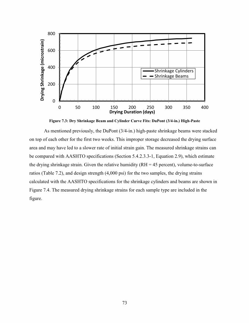
Figure 7.3: Dry Shrinkage Beam and Cylinder Curve Fits: DuPont (3/4-in.) High-Paste
As mentioned previously, the DuPont (3/4-in.) high-paste shrinkage beams were stacked
on top of each other for the first two weeks. This improper storage decreased the drying surface
area and may have led to a slower rate of initial strain gain. The measured shrinkage strains can
be compared with AASHTO specifications (Section 5.4.2.3.3-1, Equation 2.9), which estimate
the drying shrinkage strain. Given the relative humidity (RH = 45 percent), volume-to-surface
ratios (Table 7.2), and design strength (4,000 psi) for the two samples, the drying strains
calculated with the AASHTO specifications for the shrinkage cylinders and beams are shown in
Figure 7.4. The measured drying shrinkage strains for each sample type are included in the
figure.
0
200
400
600
800
0 50 100 150 200 250 300 350 400
Dryi
ng S
hrin
kage
(mic
rost
rain
)
Drying Duration (days)
Shrinkage CylindersShrinkage Beams
73
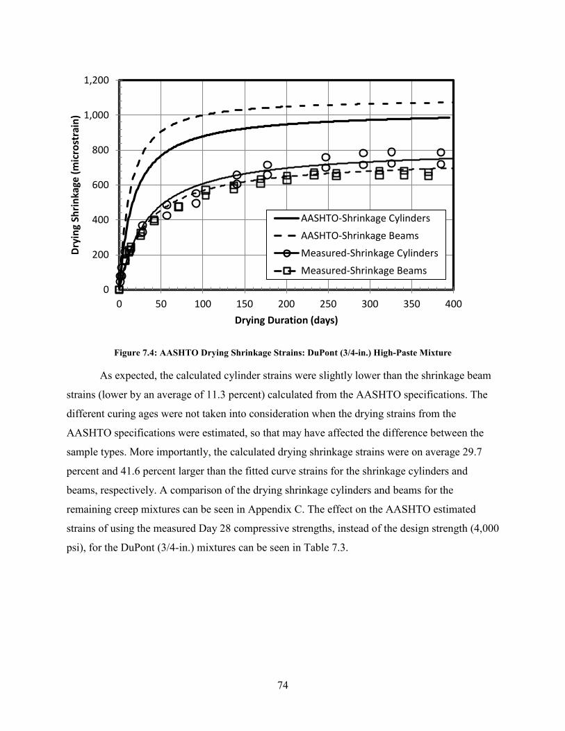
Figure 7.4: AASHTO Drying Shrinkage Strains: DuPont (3/4-in.) High-Paste Mixture
As expected, the calculated cylinder strains were slightly lower than the shrinkage beam
strains (lower by an average of 11.3 percent) calculated from the AASHTO specifications. The
different curing ages were not taken into consideration when the drying strains from the
AASHTO specifications were estimated, so that may have affected the difference between the
sample types. More importantly, the calculated drying shrinkage strains were on average 29.7
percent and 41.6 percent larger than the fitted curve strains for the shrinkage cylinders and
beams, respectively. A comparison of the drying shrinkage cylinders and beams for the
remaining creep mixtures can be seen in Appendix C. The effect on the AASHTO estimated
strains of using the measured Day 28 compressive strengths, instead of the design strength (4,000
psi), for the DuPont (3/4-in.) mixtures can be seen in Table 7.3.
0
200
400
600
800
1,000
1,200
0 50 100 150 200 250 300 350 400
Dryi
ng S
hrin
kage
(mic
rost
rain
)
Drying Duration (days)
AASHTO-Shrinkage CylindersAASHTO-Shrinkage BeamsMeasured-Shrinkage CylindersMeasured-Shrinkage Beams
74

Table 7.3: AASHTO Strains from Measured Strengths: DuPont (3/4-in.) Mixtures
f'28 Fitted 𝛆𝟑𝟔𝟔𝟓
(microstrain)
Predicted 𝛆𝟑𝟔𝟔𝟓
(microstrain)
𝛆𝟑𝟔𝟔𝟓 Difference (microstrain)
Difference (%)
High-Paste 6,530 690 670 20 2.9% Low-Paste 4,400 650 980 330 33.7% High-Strength 6,040 630 720 90 12.5% Low-Strength 3,750 760 1,140 380 33.3%
The accuracy of the Day 365 AASHTO drying shrinkage strains improved when the
measured Day 28 strengths for the DuPont (3/4-in.) high-paste and high-strength mixtures were
used. The low-paste and low-strength mixtures were over-predicted by an average of 33.5
percent by the AASHTO specifications. The results from the AASHTO specifications for
estimating the drying shrinkage did not match the measured drying shrinkage values when the
measured strengths were used. The accuracy of the formula might be improved by accounting for
the effects of paste content, water-cementitious ratio, and measured compressive strength of the
concrete mixtures.
The fitted Day 365 strains from the DuPont (3/4-in.) mixtures are plotted against the
water-cementitious ratio and paste content for the laboratory mixtures in Figure 7.5 and Figure
7.6, respectively. As expected, the fitted Day 365 drying shrinkage strains increased with an
increase in water-cementitious ratio, as well as an increase in paste content.
75
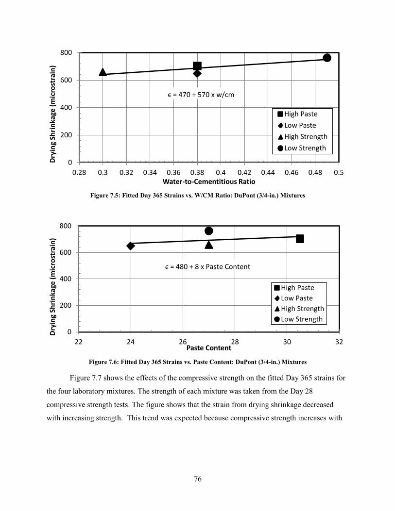
Figure 7.5: Fitted Day 365 Strains vs. W/CM Ratio: DuPont (3/4-in.) Mixtures
Figure 7.6: Fitted Day 365 Strains vs. Paste Content: DuPont (3/4-in.) Mixtures
Figure 7.7 shows the effects of the compressive strength on the fitted Day 365 strains for
the four laboratory mixtures. The strength of each mixture was taken from the Day 28
compressive strength tests. The figure shows that the strain from drying shrinkage decreased
with increasing strength. This trend was expected because compressive strength increases with
0
200
400
600
800
0.28 0.3 0.32 0.34 0.36 0.38 0.4 0.42 0.44 0.46 0.48 0.5
Dryi
ng S
hrin
kage
(mic
rost
rain
)
Water-to-Cementitious Ratio
High PasteLow PasteHigh StrengthLow Strength
ϵ = 470 + 570 x w/cm
0
200
400
600
800
22 24 26 28 30 32
Dryi
ng S
hrin
kage
(mic
rost
rain
)
Paste Content
High PasteLow PasteHigh StrengthLow Strength
ϵ = 480 + 8 x Paste Content
76
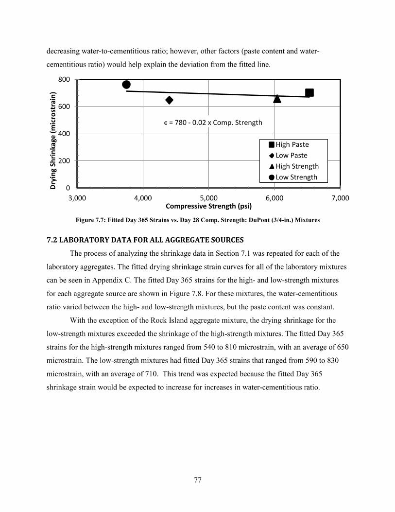
decreasing water-to-cementitious ratio; however, other factors (paste content and water-
cementitious ratio) would help explain the deviation from the fitted line.
Figure 7.7: Fitted Day 365 Strains vs. Day 28 Comp. Strength: DuPont (3/4-in.) Mixtures
7.2 LABORATORY DATA FOR ALL AGGREGATE SOURCES
The process of analyzing the shrinkage data in Section 7.1 was repeated for each of the
laboratory aggregates. The fitted drying shrinkage strain curves for all of the laboratory mixtures
can be seen in Appendix C. The fitted Day 365 strains for the high- and low-strength mixtures
for each aggregate source are shown in Figure 7.8. For these mixtures, the water-cementitious
ratio varied between the high- and low-strength mixtures, but the paste content was constant.
With the exception of the Rock Island aggregate mixture, the drying shrinkage for the
low-strength mixtures exceeded the shrinkage of the high-strength mixtures. The fitted Day 365
strains for the high-strength mixtures ranged from 540 to 810 microstrain, with an average of 650
microstrain. The low-strength mixtures had fitted Day 365 strains that ranged from 590 to 830
microstrain, with an average of 710. This trend was expected because the fitted Day 365
shrinkage strain would be expected to increase for increases in water-cementitious ratio.
0
200
400
600
800
3,000 4,000 5,000 6,000 7,000
Dryi
ng S
hrin
kage
(mic
rost
rain
)
Compressive Strength (psi)
High PasteLow PasteHigh StrengthLow Strength
ϵ = 780 - 0.02 x Comp. Strength
77

Figure 7.8: Fitted Day 365 Drying Shrinkage Strain: High- and Low-Strength Mixtures
Figure 7.9 shows the fitted Day 365 strain values of each of the aggregate sources for the
high- and low-paste mixtures. The water-cementitious ratio was the same for both the high- and
low-paste mixtures, and only the paste content varied.
Figure 7.9: Fitted Day 365 Drying Shrinkage Strain: High- and Low-Paste Mixtures
As expected, increasing the paste content generally increased the drying shrinkage for the
mixture. With the exclusion of the Santosh aggregate, the high-paste mixtures had larger fitted
Day 365 strain values than the corresponding low-paste mixtures. The fitted Day 365 strain for
0
200
400
600
800
1,000
DuPont(3/4")
DuPont(3/8")
OkanoganValley
SullivanRoad
Pasco Rock Island Santosh
Dryi
ng S
hrin
kage
(mic
rost
rain
) High StrengthLow Strength
0
200
400
600
800
1,000
DuPont(3/4")
DuPont(3/8")
OkanoganValley
SullivanRoad
Pasco Rock Island Santosh
Dryi
ng S
hrin
kage
(mic
rost
rain
) High PasteLow Paste
78

the high-paste mixtures ranged from 640 to 860 microstrain, with an average of 720 microstrain.
The low-paste mixtures ranged from 530 to 790 microstrain, with an average of 660.
As shown by figures 7.8 and 7.9, varying the aggregate source affected the fitted Day 365
drying shrinkage strains for a given mixture. The fitted Day 365 strains from the Okanogan
Valley, Sullivan Road, Pasco, and Rock Island mixtures were similar (average of 620
microstrain). The DuPont (3/4-in.) and Santosh mixtures had average fitted Day 365 strains of
700 and 780 microstrain, respectively. The DuPont (3/8-in.) mixtures had the largest fitted Day
365 strains with an average of 830 microstrain, as expected because of the higher paste contents
for the smaller aggregate size.
The high- and low-paste mixtures from the DuPont (3/4-in.), DuPont (3/8-in.), and
Sullivan Road aggregates were monitored for creep testing. Those creep mixtures had
companion drying shrinkage cylinder that were monitored in the same room as the drying
shrinkage beams. The drying shrinkage cylinders strains were normalized and fit to Equation 7.1.
The optimized coefficients and fitted Day 365 strains are listed for the shrinkage cylinders in
Table 7.4. The corresponding coefficients and fitted Day 365 strains for the drying shrinkage
beams are listed in Table 7.5. The strains from the shrinkage cylinders and beams were plotted
together for the high- and low-paste mixtures. These plots are shown in Figure 7.10 for the
DuPont (3/4-in.) aggregate, Figure 7.11 for the DuPont (3/8-in.) aggregate, and Figure 7.12 for
the Sullivan Road aggregate.
Note – The drying shrinkage beam samples for the DuPont (3/4-in.) high-paste mixture
were stored improperly for the first two weeks, as mentioned in Section 7.1.
Table 7.4: Optimized Coefficients for Shrinkage Cylinders: All Creep Mixtures
𝐭𝟓𝟎 (Days)
𝛆𝐔𝐥𝐭 (microstrain)
𝐅𝐢𝐭𝐭𝐞𝐝 𝛆𝟑𝟔𝟔𝟓 (microstrain) 𝛆𝟐𝟖 / 𝛆𝟑𝟔𝟔𝟓
DuPont (3/4") –HP 34.5 790 750 0.49 DuPont (3/4") –LP 21.6 550 520 0.61 DuPont (3/8") –HP 23.4 840 790 0.58 DuPont (3/8") –LP 26.1 700 650 0.54 Sullivan Road –HP 28.2 660 620 0.57 Sullivan Road –LP 32.7 640 590 0.53
79
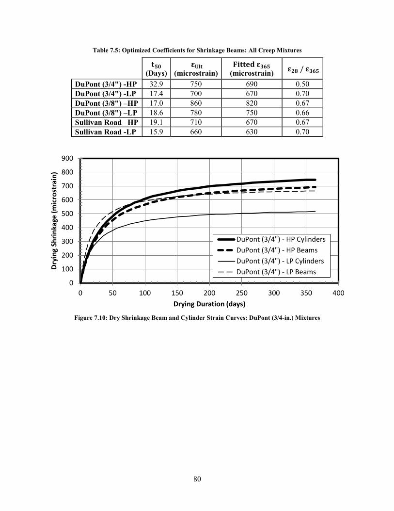
Table 7.5: Optimized Coefficients for Shrinkage Beams: All Creep Mixtures
𝐭𝟓𝟎 (Days)
𝛆𝐔𝐥𝐭 (microstrain)
𝐅𝐢𝐭𝐭𝐞𝐝 𝛆𝟑𝟔𝟔𝟓 (microstrain) 𝛆𝟐𝟖 / 𝛆𝟑𝟔𝟔𝟓
DuPont (3/4") -HP 32.9 750 690 0.50 DuPont (3/4") -LP 17.4 700 670 0.70 DuPont (3/8") –HP 17.0 860 820 0.67 DuPont (3/8") –LP 18.6 780 750 0.66 Sullivan Road –HP 19.1 710 670 0.67 Sullivan Road -LP 15.9 660 630 0.70
Figure 7.10: Dry Shrinkage Beam and Cylinder Strain Curves: DuPont (3/4-in.) Mixtures
0
100
200
300
400
500
600
700
800
900
0 50 100 150 200 250 300 350 400
Dryi
ng S
hrin
kage
(mic
rost
rain
)
Drying Duration (days)
DuPont (3/4") - HP CylindersDuPont (3/4") - HP BeamsDuPont (3/4") - LP CylindersDuPont (3/4") - LP Beams
80

Figure 7.11: Dry Shrinkage Beam and Cylinder Strain Curves: DuPont (3/8-in.) Mixtures
Figure 7.12: Drying Shrinkage Beam and Cylinder Strain Curves: Sullivan Road Mixtures
As expected, the shrinkage strains for the high-paste mixtures exceeded the strains for the
low-paste mixtures for both the drying shrinkage beams and cylinders. For the DuPont (3/8-in.)
0
100
200
300
400
500
600
700
800
900
0 50 100 150 200 250 300 350 400
Dryi
ng S
hrin
kage
(mic
rost
rain
)
Drying Duration (days)
DuPont (3/8') - HP CylindersDuPont (3/8') - HP BeamsDuPont (3/8') - LP CylindersDuPont (3/8') - LP Beams
0
100
200
300
400
500
600
700
800
900
0 50 100 150 200 250 300 350 400
Dryi
ng S
hrin
kage
(mic
rost
rain
)
Drying Duration (days)
Sullivan Road - HP CylindersSullivan Road - HP BeamsSullivan Road - LP CylindersSullivan Road - LP Beams
81

and Sullivan Road mixtures, the strains from the shrinkage beams had a faster initial rate of
strain gain than the shrinkage cylinders. After a year’s duration, the Day 365 fitted drying strains
from all of the shrinkage cylinders were on average 14.2 percent lower than the drying strains for
the shrinkage beams. This difference is consistent for the effect of the volume-to-surface as
expected from AASHTO specifications (5.4.2.3-3-1) [average difference of 11.1 percent].
According to the specifications, the difference in shrinkage strains for the two V/S ratios would
be expected to be 8.1 percent.
7.3 DATA FOR FIELD SAMPLES
The shrinkage results for the field mixtures were fit to Equation 7.1 following the same
method as that outlined in Section 7.1. The mixture proportions, fitted Day 365 strains, and
optimized constants (t50 and ϵ Ult.) for the different field mixtures are listed in Table 7.6. Figure
7.13 is a plot of the fitted curves for the field mixtures.
Table 7.6: Optimized Constants for Field Mixtures
Paste Content (%)
W/CM Ratio
𝐭𝟓𝟎 (Days)
𝛆𝐔𝐥𝐭 (microstrain)
𝐅𝐢𝐭𝐭𝐞𝐝 𝛆𝟑𝟔𝟔𝟓 (microstrain) 𝛆𝟐𝟖 / 𝛆𝟑𝟔𝟔𝟓
Freya to Farewell 25.5 0.31 18.0 820 820 0.64 Alaskan Way 25.2 0.31 13.6 710 720 0.70 Tumwater Canyon 25.9* 0.40* 8.3 830 870 0.80 Snohomish 24.6 0.32 12.5 860 870 0.72 Camas / Washougal 27.8 0.41 17.6 1,090 1,060 0.64
* Tumwater Canyon mixture included fly ash.
82
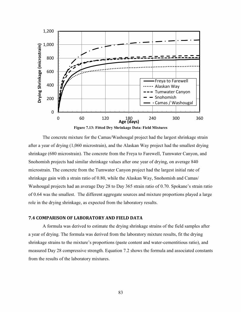
Figure 7.13: Fitted Dry Shrinkage Data: Field Mixtures
The concrete mixture for the Camas/Washougal project had the largest shrinkage strain
after a year of drying (1,060 microstrain), and the Alaskan Way project had the smallest drying
shrinkage (680 microstrain). The concrete from the Freya to Farewell, Tumwater Canyon, and
Snohomish projects had similar shrinkage values after one year of drying, on average 840
microstrain. The concrete from the Tumwater Canyon project had the largest initial rate of
shrinkage gain with a strain ratio of 0.80, while the Alaskan Way, Snohomish and Camas/
Washougal projects had an average Day 28 to Day 365 strain ratio of 0.70. Spokane’s strain ratio
of 0.64 was the smallest. The different aggregate sources and mixture proportions played a large
role in the drying shrinkage, as expected from the laboratory results.
7.4 COMPARISON OF LABORATORY AND FIELD DATA
A formula was derived to estimate the drying shrinkage strains of the field samples after
a year of drying. The formula was derived from the laboratory mixture results, fit the drying
shrinkage strains to the mixture’s proportions (paste content and water-cementitious ratio), and
measured Day 28 compressive strength. Equation 7.2 shows the formula and associated constants
from the results of the laboratory mixtures.
0
200
400
600
800
1,000
1,200
0 60 120 180 240 300 360
Dryi
ng S
hrin
kage
(mic
rost
rain
)
Age (days)
Freya to FarewellAlaskan WayTumwater CanyonSnohomishCamas / Washougal
83
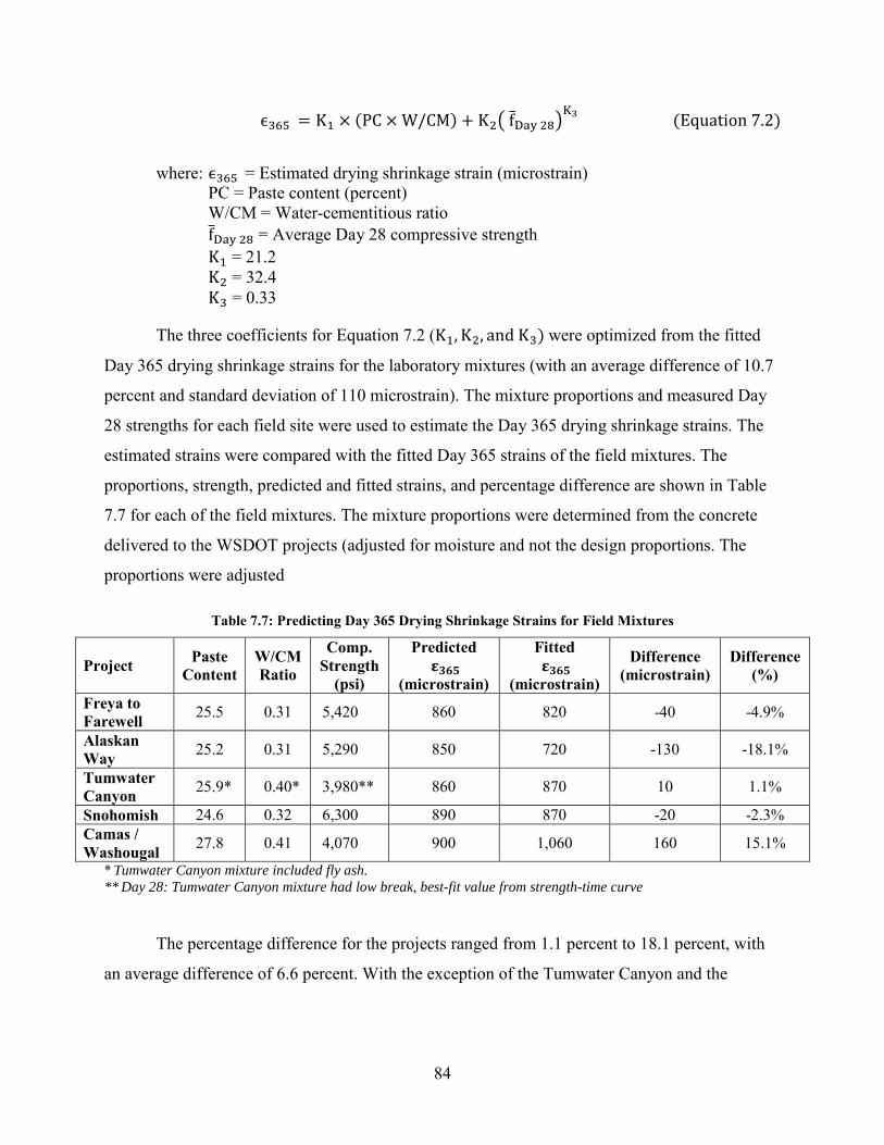
ϵ365 = K1 × (PC × W/CM) + K2� fD̅ay 28�K3 (Equation 7.2)
where: ϵ365 = Estimated drying shrinkage strain (microstrain) PC = Paste content (percent) W/CM = Water-cementitious ratio fD̅ay 28 = Average Day 28 compressive strength
K1 = 21.2 K2 = 32.4 K3 = 0.33
The three coefficients for Equation 7.2 (K1, K2, and K3) were optimized from the fitted
Day 365 drying shrinkage strains for the laboratory mixtures (with an average difference of 10.7
percent and standard deviation of 110 microstrain). The mixture proportions and measured Day
28 strengths for each field site were used to estimate the Day 365 drying shrinkage strains. The
estimated strains were compared with the fitted Day 365 strains of the field mixtures. The
proportions, strength, predicted and fitted strains, and percentage difference are shown in Table
7.7 for each of the field mixtures. The mixture proportions were determined from the concrete
delivered to the WSDOT projects (adjusted for moisture and not the design proportions. The
proportions were adjusted
Table 7.7: Predicting Day 365 Drying Shrinkage Strains for Field Mixtures
Project Paste Content
W/CM Ratio
Comp. Strength
(psi)
Predicted 𝛆𝟑𝟔𝟔𝟓
(microstrain)
Fitted 𝛆𝟑𝟔𝟔𝟓
(microstrain)
Difference (microstrain)
Difference (%)
Freya to Farewell 25.5 0.31 5,420 860 820 -40 -4.9%
Alaskan Way 25.2 0.31 5,290 850 720 -130 -18.1%
Tumwater Canyon 25.9* 0.40* 3,980** 860 870 10 1.1%
Snohomish 24.6 0.32 6,300 890 870 -20 -2.3% Camas / Washougal 27.8 0.41 4,070 900 1,060 160 15.1%
* Tumwater Canyon mixture included fly ash. ** Day 28: Tumwater Canyon mixture had low break, best-fit value from strength-time curve
The percentage difference for the projects ranged from 1.1 percent to 18.1 percent, with
an average difference of 6.6 percent. With the exception of the Tumwater Canyon and the
84

Camas/Washougal projects, the predicted strains were lower than the actual strains. The
constants derived for Equation 7.2 were based on the average results from all of the laboratory
mixtures to avoid any aggregate-specific effects. As shown in Figure 7.13, the fitted drying
shrinkage curves for the Alaskan Way and Camas/Washougal projects are significantly different
than those for the other field mixtures. These results are consistent with the percentage
differences listed in Table 7.6. The accuracy of the estimated Day 365 drying shrinkage strains
varied with each field mixture, but with an average difference of 6.6 percent from the fitted and
estimated strains, Equation 7.2 has the potential for future usage. By making further laboratory
mixtures that vary the proportions and aggregate sources, the accuracy of Equation 7.2 may be
improved.
7.5 SHRINKAGE CURVE VARIABILITY
This section investigates the effects of varying the monitored duration of drying
shrinkage samples on the accuracy of the extrapolated shrinkage at one year. Six drying
durations were selected to analyze the error in extrapolating the shrinkage at a year’s length. To
show typical results, the shrinkage data from DuPont (3/4-in.) low-strength mixture was fit to
Equation 7.1 for drying durations of 28, 56, 90, 180, 270, and 365 days. The percentage
difference between the extrapolated and measured fitted strain for a year’s duration were
averaged and are listed in Table 7.8. The differences in fitted Day 365 strains values are included
in the table. The fitted curves from each of the different drying durations are shown in Figure
7.14.
Table 7.8: Percentage Difference from Varying Drying Shrinkage Monitor Durations
Monitored Duration (days)
Fitted 𝛆𝟑𝟔𝟔𝟓 (percentage difference)
Average Strains (percentage difference)
270 2.1% 1.2% 180 3.0% 4.2% 90 5.6% 6.8% 56 14.9% 9.6% 28 32.5% 20.7%
85
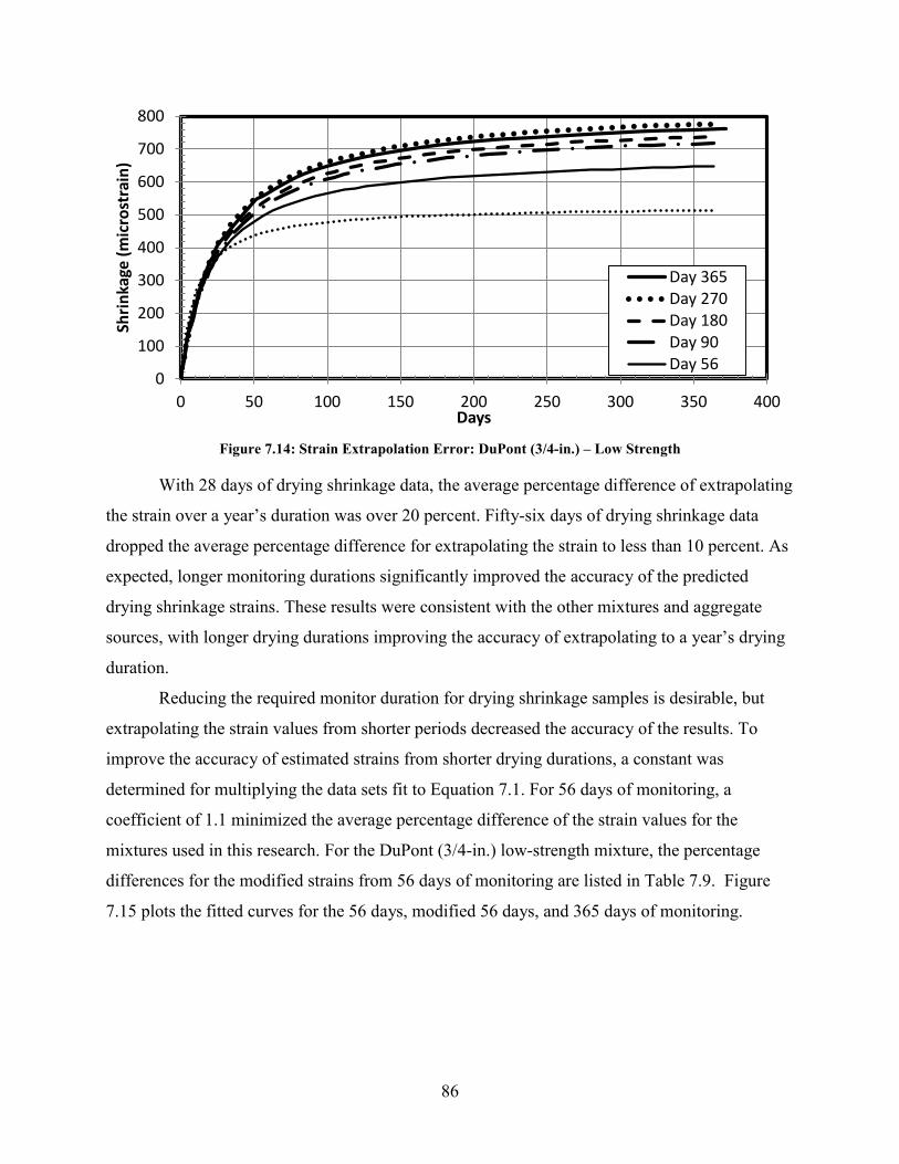
Figure 7.14: Strain Extrapolation Error: DuPont (3/4-in.) – Low Strength
With 28 days of drying shrinkage data, the average percentage difference of extrapolating
the strain over a year’s duration was over 20 percent. Fifty-six days of drying shrinkage data
dropped the average percentage difference for extrapolating the strain to less than 10 percent. As
expected, longer monitoring durations significantly improved the accuracy of the predicted
drying shrinkage strains. These results were consistent with the other mixtures and aggregate
sources, with longer drying durations improving the accuracy of extrapolating to a year’s drying
duration.
Reducing the required monitor duration for drying shrinkage samples is desirable, but
extrapolating the strain values from shorter periods decreased the accuracy of the results. To
improve the accuracy of estimated strains from shorter drying durations, a constant was
determined for multiplying the data sets fit to Equation 7.1. For 56 days of monitoring, a
coefficient of 1.1 minimized the average percentage difference of the strain values for the
mixtures used in this research. For the DuPont (3/4-in.) low-strength mixture, the percentage
differences for the modified strains from 56 days of monitoring are listed in Table 7.9. Figure
7.15 plots the fitted curves for the 56 days, modified 56 days, and 365 days of monitoring.
0
100
200
300
400
500
600
700
800
0 50 100 150 200 250 300 350 400
Shrin
kage
(mic
rost
rain
)
Days
Day 365Day 270Day 180Day 90Day 56
86

Table 7.9: Improvement from Modified Drying Shrinkage: DuPont (3/4-in.) Low-Strength
Fitted 𝛆𝟑𝟔𝟔𝟓 (percentage difference)
Average Strains (percentage difference)
Modified 56 2.2% 4.7% Unmodified Day 56 14.9% 9.6%
Figure 7.15: Modified Drying Shrinkage Strain: DuPont (3/4-in.) Low-Strength
The results from modifying the fitted drying shrinkage curve for 56 days of monitoring
were consistent for the remaining laboratory and field mixtures. Using a coefficient of 1.1 to
multiply the fitted shrinkage strain curves from 56 days of monitoring improved the extrapolated
strain values at a year’s duration of monitoring. The percentage differences in fitted Day 365
strains and average strain value for the modified and unmodified Day 56 drying shrinkage curve
fits are listed in Table 7.10.
0
100
200
300
400
500
600
700
800
0 50 100 150 200 250 300 350 400
Shrin
kage
(mic
rost
rain
)
Days
Day 365Modified Day 56Day 56
87
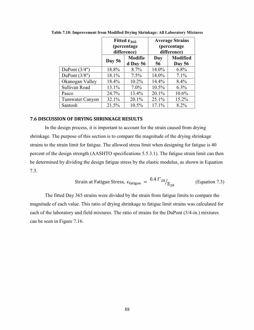
Table 7.10: Improvement from Modified Drying Shrinkage: All Laboratory Mixtures
Fitted 𝛆𝟑𝟔𝟔𝟓 (percentage difference)
Average Strains (percentage difference)
Day 56 Modified Day 56
Day 56
Modified Day 56
DuPont (3/4") 18.8% 8.7% 14.0% 6.8% DuPont (3/8") 18.1% 7.5% 14.0% 7.1% Okanogan Valley 18.4% 10.2% 14.4% 8.4% Sullivan Road 13.1% 7.0% 10.5% 6.3% Pasco 24.7% 13.4% 20.1% 10.6% Tumwater Canyon 32.1% 20.1% 25.1% 15.2% Santosh 21.5% 10.5% 17.1% 8.2%
7.6 DISCUSSION OF DRYING SHRINKAGE RESULTS
In the design process, it is important to account for the strain caused from drying
shrinkage. The purpose of this section is to compare the magnitude of the drying shrinkage
strains to the strain limit for fatigue. The allowed stress limit when designing for fatigue is 40
percent of the design strength (AASHTO specifications 5.5.3.1). The fatigue strain limit can then
be determined by dividing the design fatigue stress by the elastic modulus, as shown in Equation
7.3.
Strain at Fatigue Stress, ϵfatigue = 0.4 f ′28E28� (Equation 7.3)
The fitted Day 365 strains were divided by the strain from fatigue limits to compare the
magnitude of each value. This ratio of drying shrinkage to fatigue limit strains was calculated for
each of the laboratory and field mixtures. The ratio of strains for the DuPont (3/4-in.) mixtures
can be seen in Figure 7.16.
88

Figure 7.16: Day 28 Drying Strain to Fatigue Strain: DuPont (3/4-in.) Mixtures
The fitted Day 365 drying shrinkage strains were on average twice as large as the elastic
strain at the fatigue stress. This calculation illustrates the significance of the drying shrinkage.
These results were consistent throughout the laboratory mixtures, as shown in Figure 7.17 for the
high- and low-strength mixtures and in Figure 7.18 for and high- and low-paste mixtures.
0.0
0.4
0.8
1.2
1.6
2.0
2.4
High Paste Low Paste High Strength Low Strength
Dryi
ng S
hrin
kage
/ A
ASHT
O F
atig
ue S
trai
n
89

Figure 7.17: Drying Strain to Fatigue Strain: All Aggregates-High- and Low-Strength
Figure 7.18: Drying Strain to Fatigue Strain: All Aggregates-High- and Low-Paste
0.0
0.4
0.8
1.2
1.6
2.0
2.4
DuPont(3/4")
DuPont(3/8")
OkanoganValley
SullivanRoad
Pasco Rock Island Santosh
Dryi
ng S
hrin
kage
/ A
ASHT
O F
atig
ue S
trai
n High StrengthLow Strength
0.0
0.4
0.8
1.2
1.6
2.0
2.4
DuPont(3/4")
DuPont(3/8")
OkanoganValley
SullivanRoad
Pasco Rock Island Santosh
Dryi
ng S
hrin
kage
/ A
ASHT
O F
atig
ue S
trai
n
High PasteLow Paste
90

7.6 ANALYSIS OF DRYING SHRINKAGE RESULTS
The results presented in this chapter led to the following observations:
• Variations in the aggregate type significantly affected the drying shrinkage strains
(figures 7.8, 7.9, 7.17 and 7.18).
• The drying shrinkage strains increased with increasing paste content (figures 7.6 and 7.9).
• Increases in the water-cementitious ratio increased the drying shrinkage strain (figures
7.5 and 7.8).
• Increasing compressive strengths decreased drying shrinkage strains (Figure 7.7).
• Increases in the volume-to-surface ratios of drying shrinkage samples decreased the
initial rate of shrinkage strain gain (figures 7.3, 7.4, 7.10, 7.11 and 7.12).
Equation 7.1 did a great job at fitting the monitored drying shrinkage strains (Figure 7.1).
AASHTO specifications (5.1.2.3.3-1, Equation 2.9) did not estimate the drying shrinkage strains
well (Figure 7.4). The long-term shrinkage can be predicted from short-term shrinkage
monitoring, with greater accuracy than AASHTO predictions, by multiplying monitored
shrinkage curves by an extrapolation correction coefficient. For only 56 days of monitoring,
extrapolated drying shrinkage strains for a year’s duration were improved by multiplying by a
constant of 1.1 (Figure 7.15). The accuracy of the extrapolated drying shrinkage strains were
within an average of 8.9 percent difference of the strain curves from 365 days of monitoring.
Another method of estimating the Day 365 drying shrinkage strains is to use Equation
7.2. This formula accounts for the mixture proportions (paste content and water-cementitious
ratio) and measured Day 28 compressive strengths to estimate the Day 365 drying shrinkage
strains. Aggregate source does affect the accuracy of the estimated strain values (Table 7.7), but
further research for specific aggregate sources would vary the optimized values (K1, K2, and
K3), and could improve the accuracy of the equation.
91
Chapter 8: Creep
This chapter reports the results of a test program (Section 3.4.5) that was designed to
measure the elastic strains, creep strains (composed of basic and drying creep strains), and drying
shrinkage strains on six sets of samples. Creep tests were conducted for three aggregate types
(DuPont 3/4-in., DuPont Pea Gravel, and Sullivan Road) for both high- and low-paste contents.
For each combination of aggregate type and paste content, sealed and unsealed cylinders were
loaded to approximately 35 percent of the Day 14 failure stress and then monitored for over one
year. In parallel, unloaded, unsealed cylinders were monitored to measure the drying shrinkage.
The following procedure was used to determine the elastic, creep, and drying shrinkage
strains for each creep rig. Since it took around five minutes to load and measure the creep
samples, the initial lengths of each set of gauges were extrapolated from the measured data
(Appendix D) back to a time of zero. The elastic deformations of the loaded creep cylinders
(sealed and unsealed) were as assumed to be the difference between the length immediately after
applying the axial load and the initial, extrapolated lengths (8.1.1 and 8.2.1). The monitored
deformations of the creep and drying shrinkage cylinders were divided by the respective initial
lengths to calculate the long-term strains, which were then fit to a nonlinear curve (8.1.2 and
8.2.2). Those data sets were then used to analyze the drying shrinkage (8.1.4 and 8.2.3), as well
as the creep performance (8.1.5 and 8.2.4) in terms of specific creep (8.1.6 and 8.2.5) and creep
coefficient (8.1.7 and 8.2.6).
The process followed to analyze the deformation data is illustrated in Section 8.1 for the
DuPont (3/4-in.), high-paste mixture. The results of applying the same methodology to the data
for all samples are reported in Section 8.2. During the data analysis, the researchers discovered
that the integrity of the sealant on the sealed creep cylinders may have been compromised. This
issue, and its effects on the calculation of basic and drying creep strains, is discussed in Section
8.1.3. Appendix E provides the details of the creep data.
8.1 LABORATORY DATA FOR DUPONT (3/4-IN.) HIGH-PASTE MIXTURE
The analysis procedure used to process the data is illustrated in this section by using
deformation data for the DuPont (3/4-in.) high-paste mixture.
92

8.1.1 Elastic Strain
At Day 14, each creep rig was loaded to approximately 35 percent of the Day 14 failure
stress. The initial strain due to loading is defined as the elastic strain. Because of the non-
homogeneity of the cylinder, the load on each creep rig may not have been applied exactly at the
cylinder’s centroid. Variations in measured strains among the four gauges were expected.
To evaluate whether the variation in measured elastic strains among a set of gauges were
sufficiently consistent for a single cylinder, a procedure was established to quantify any
discrepancy, and when necessary, to modify the data. For each gauge, the discrepancy between
this gauge and the others was determined by extrapolating a plane defined by the strains
measured by the other three gauges. The discrepancy was estimated as the difference between
the fourth gauge’s strain and the planar projection at that location based on the other three
gauges. This process was repeated by varying the strain gauge that was excluded when forming
the strain plane. If the difference between the measured and projected strains exceeded 100
microstrain, then the error was classified as excessive, and corrective action was taken.
To improve the data set, the centroid of the strain plane was found for the cylinder by
calculating the average measured strain of the four gauges. The gauge with the largest difference
between the measured and average strains was altered to the value calculated by the strain plane
from the remaining three gauges. This procedure had the effect of eliminating the data point with
the largest discrepancy.
Table 8.1 lists the initial elastic strains measured for each of the four sets of gauges
(labeled North, South, East, or West, depending on the gauge orientation) on the loaded,
unsealed creep cylinders. This data set had only one data point (out of eight) that had a large
discrepancy. Specifically, the West gauge on unsealed Cylinder #2 had a discrepancy of 440
microstrain, so the elastic strain was altered (to the value shown in parentheses).
93

Table 8.1: Measured Elastic Strain and Modulus: DuPont (3/4-in.) High-Paste Mixture
Measured Elastic Strain (microstrain)
Unsealed Cylinder #1
Unsealed Cylinder #2 Average
North Gauge 310 340 330 West Gauge 340 730 (290) 320 East Gauge 380 460 420 South Gauge 410 410 410
Average Strain 360 380 370 Applied Stress (psi) 1,760 1,860 1,810
The mean elastic strain (with the modification of unsealed Cylinder #2, West gauge) from
the creep rig and the Day 14 elastic modulus from standardized testing (ASTM C469) were used
to estimate the actual applied stress on each creep mixture as shown in Equation 8.1.
f ̅14 creep = εElastic × E�14 (Equation 8.1)
where: E� 14 = 4,990 ksi (Table 6.1) εElastic = 370 microstrain
For this mixture, f1̅4 creep was estimated as 1,810 psi. This calculated applied stress from
the creep samples was compared with the targeted stress value of 35 percent of the Day 14
failure stress. As shown in Table 4.1 for the DuPont (3/4-in.) high-paste mixture, the Day 14
compressive strength was 4,900 psi, which resulted in a targeted stress of 1,750 psi. Therefore,
the inferred average stress for the creep samples (1,810 psi) was 8.4 percent larger than that
inferred from standard elastic modulus testing. The difference in stresses may have arisen from
inaccuracies in the applied stress on the creep rig, the measured deformation, and the
extrapolation of the initial lengths to account for early creep.
8.1.2 Time-Dependent Deformations
As explained in Section 3.4.5, the deformations of the loaded unsealed and sealed
cylinders, as well as the drying shrinkage cylinders, were monitored for a year. To estimate the
time-dependent deformations, the elastic deformation was subtracted from the monitored
deformations. The strains for the drying shrinkage and creep cylinders were then calculated by
94
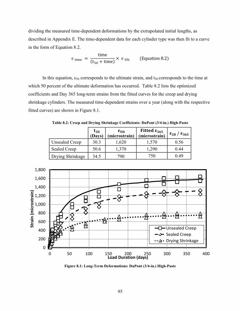
dividing the measured time-dependent deformations by the extrapolated initial lengths, as
described in Appendix E. The time-dependent data for each cylinder type was then fit to a curve
in the form of Equation 8.2.
ϵ time = time
(t50 + time) × ϵ Ult. (Equation 8.2)
In this equation, ε50 corresponds to the ultimate strain, and t50 corresponds to the time at
which 50 percent of the ultimate deformation has occurred. Table 8.2 lists the optimized
coefficients and Day 365 long-term strains from the fitted curves for the creep and drying
shrinkage cylinders. The measured time-dependent strains over a year (along with the respective
fitted curves) are shown in Figure 8.1.
Table 8.2: Creep and Drying Shrinkage Coefficients: DuPont (3/4-in.) High-Paste
𝐭𝟓𝟎
(Days) 𝛆𝐔𝐥𝐭
(microstrain) 𝐅𝐢𝐭𝐭𝐞𝐝 𝛆𝟑𝟔𝟔𝟓
(microstrain) 𝛆𝟐𝟖 / 𝛆𝟑𝟔𝟔𝟓
Unsealed Creep 30.3 1,620 1,570 0.56 Sealed Creep 50.6 1,370 1,290 0.44 Drying Shrinkage 34.5 790 750 0.49
Figure 8.1: Long-Term Deformations: DuPont (3/4-in.) High-Paste
0
200
400
600
800
1,000
1,200
1,400
1,600
1,800
0 50 100 150 200 250 300 350 400
Stra
in (m
icro
stra
in)
Load Duration (days)
Unsealed CreepSealed CreepDrying Shrinkage
95
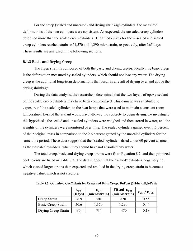
For the creep (sealed and unsealed) and drying shrinkage cylinders, the measured
deformations of the two cylinders were consistent. As expected, the unsealed creep cylinders
deformed more than the sealed creep cylinders. The fitted curves for the unsealed and sealed
creep cylinders reached strains of 1,570 and 1,290 microstrain, respectively, after 365 days.
These results are analyzed in the following sections.
8.1.3 Basic and Drying Creep
The creep strain is composed of both the basic and drying creeps. Ideally, the basic creep
is the deformation measured by sealed cylinders, which should not lose any water. The drying
creep is the additional long-term deformations that occur as a result of drying over and above the
drying shrinkage.
During the data analysis, the researchers determined that the two layers of epoxy sealant
on the sealed creep cylinders may have been compromised. This damage was attributed to
exposure of the sealed cylinders to the heat lamps that were used to maintain a constant room
temperature. Loss of the sealant would have allowed the concrete to begin drying. To investigate
this hypothesis, the sealed and unsealed cylinders were weighed and then stored in water, and the
weights of the cylinders were monitored over time. The sealed cylinders gained over 1.5 percent
of their original mass in comparison to the 2.6 percent gained by the unsealed cylinders for the
same time period. These data suggest that the “sealed” cylinders dried about 60 percent as much
as the unsealed cylinders, when they should have not absorbed any water.
The total creep, basic and drying creep strains were fit to Equation 8.2, and the optimized
coefficients are listed in Table 8.3. The data suggest that the “sealed” cylinders began drying,
which caused larger strains than expected and resulted in the drying creep strain to become a
negative value, which is not credible.
Table 8.3: Optimized Coefficients for Creep and Basic Creep: DuPont (3/4-in.) High-Paste
𝐭𝟓𝟎 (Days)
𝛆𝐔𝐥𝐭 (microstrain)
𝐅𝐢𝐭𝐭𝐞𝐝 𝛆𝟑𝟔𝟔𝟓 (microstrain) 𝛆𝟐𝟖 / 𝛆𝟑𝟔𝟔𝟓
Creep Strain 26.9 880 820 0.55 Basic Creep Strain 50.6 1,370 1,290 0.44 Drying Creep Strain 159.1 -710 -470 0.18
96

The rest of this chapter focuses on the behavior of the unsealed cylinders because the
moisture conditions for the “sealed” cylinders are unknown.
8.1.4 Drying Shrinkage
The unloaded, unsealed cylinders had a drying shrinkage strain of 750 microstrain from
the fitted curve after a year of monitoring. As mentioned in Section 7.1, the fitted drying
shrinkage curves for the DuPont (3/4-in.) high-paste cylinders and beams were compared to
evaluate the effects of varying the curing duration before air drying and the volume-to-surface
ratio. The fitted Day 365 strain for the shrinkage cylinders exceeded the fitted Day 365 strain for
the beams by 8.3 percent. This suggests that the shorter curing period had a greater effect than
the larger volume-to-surface ratio.
An analysis of AASHTO specifications (5.4.2.3.3-1, Equation 2.9) was also performed
(Section 7.1) for the drying shrinkage cylinder and beam samples of the DuPont (3/4-in.) high-
paste mixture. The AASHTO specifications estimate the drying shrinkage strains for a concrete
sample on the basis of the relative humidity, volume-to-surface ratio, design strength, and drying
duration. Using the conditions present for this research, drying shrinkage curves were evaluated
for the shrinkage beams and cylinders and were compared with the measured values. The
calculated drying shrinkage strains were on average 29.7 percent and 41.6 percent larger than the
fitted curve strains for the shrinkage cylinders and beams, respectively.
8.1.5 Creep Strains
The creep strains were determined by subtracting the drying shrinkage and elastic strains
from the monitored strains of the unsealed, loaded cylinders. The creep-strain data were fit to
Equation 8.2, and the optimized coefficients and fitted Day 365 strain are listed in Table 8.4. The
total time-dependent strain (result of subtracting the elastic strain from the unsealed, loaded
cylinder) and drying shrinkage strain are included in the table for comparison. Figure 8.2 plots
the fitted strain curves for the total time-dependent, drying shrinkage, and creep strains.
97
Table 8.4: Optimized Constants for DuPont (3/4-in.) High-Paste Mixture
𝐭𝟓𝟎 (Days)
𝛆𝐔𝐥𝐭 (microstrain)
𝐅𝐢𝐭𝐭𝐞𝐝 𝛆𝟑𝟔𝟔𝟓 (microstrain) 𝛆𝟐𝟖 / 𝛆𝟑𝟔𝟔𝟓
Total Time-Dependent Strain 30.3 1,620 1,570 0.56 Drying Shrinkage Strain 34.5 790 750 0.49
Creep Strain 26.9 880 820 0.55
Figure 8.2: Long-Term Deformation Fitted Curves: DuPont (3/4-in.) High-Paste
This figure shows that the magnitudes of creep and drying shrinkage strains were similar
for the DuPont (3/4-in.) high-paste mixture. The creep strains exceeded the drying shrinkage
strains by an average of 12.6 percent.
8.1.6 Specific Creep
The specific creep data were calculated by dividing the creep strain data by the calculated
applied stress (in psi) that was applied to each creep rig. The targeted stress on each creep rig
was 35 percent of the Day 14 failure stress (Section 3.4.5); however, the applied stress on a creep
rig may have varied and was calculated from the elastic strain measurements (Section 8.1.1).
Dividing the creep strain by the applied stress creates a normalized data set, which is defined in
ACI 209 as the specific creep. Specific creep provides a comparison of the creep strain for
concrete mixtures with different strengths and applied loads. The specific creep data were fit to
0200400600800
1,000
1,200
1,400
1,600
1,800
0 50 100 150 200 250 300 350 400
Stra
in (m
icro
stra
in)
Load Duration (days)
Total Time-Dependent StrainDrying Shrinkage StrainCreep strain
98

the curve of the form of Equation 8.2, and the optimized constants for the DuPont (3/4-in.) high-
paste mixture are reported in Table 8.5 and Figure 8.3.
Table 8.5: Optimized Coefficients for Specific Creep: DuPont (3/4-in.) High-Paste
𝐭𝟓𝟎 (Days)
Ultimate (microstrain/psi)
Fitted Day 365 (microstrain/psi) Day 28/Day 365
Specific Creep 27.0 0.45 0.43 0.55
Figure 8.3: Specific Creep Fitted Curve: DuPont (3/4-in.) High-Paste
ACI 209 recommends this method of normalization to correct for the effects of varying
strength among mixtures. Analyzing the specific creep strains from the remaining mixtures
provides a method of documenting the effects of paste content, aggregate size, and aggregate
type on the creep behavior without strength affecting the data.
8.1.7 Creep Coefficient
The creep coefficient is defined as the creep strain divided by the elastic strain at a
particular duration of loading. The DuPont (3/4-in.) high-paste creep strain was normalized with
the mean elastic strain of all four creep cylinders (370 microstrain, Table 8.1), and the resulting
fitted curve can be seen in Figure 8.4. The AASHTO specifications (5.4.2.3.2-1, Equation 2.12)
estimate a creep coefficient that varies with load duration. On the basis of the cure duration
before loading (14 days), relative humidity (RH = 45 percent), design strength of the concrete
0.0
0.1
0.2
0.3
0.4
0.5
0 50 100 150 200 250 300 350 400
Spec
ific C
reep
(mic
rost
rain
/ ps
i)
Load Duration (days)
99

(4,000 psi), and volume-to-surface ratio (V/S = 1.5), the calculated creep coefficient curve was
included in Figure 8.4.
Figure 8.4: AASHTO Predicted Creep Coefficient: DuPont (3/4-in.) High-Paste
The creep coefficients at Day 365 were 2.1 for the DuPont (3/4-in.) high-paste mixture
and 2.2 for AASHTO specifications (a difference of only 4.2 percent). This result implies that
the creep strain at one year is greater than twice the magnitude of the elastic strain for an applied
load of approximately 35 percent of the Day 14 compressive strength. The creep coefficients
estimated by AASHTO under-predicted the initial rate of strain gain of the measured creep
samples. For example, the ratio of Day 28 to Day 365 creep coefficient for the AASHTO curve
was 0.42, whereas it was 0.55 for the DuPont (3/4-in.) high-paste mixture (a difference of 24
percent).
The accuracy of creep calculations based on the creep coefficient depends greatly on the
calculated elastic deformation. To illustrate this dependence, the creep strains were determined
from elastic strain values based on three sets of assumptions:
• The first elastic strain was calculated by using the AASHTO predicted elastic modulus
(Section 5.4.2.4-1, Equation 2.7) based on the design strength of the mixture (4,000 psi)
along with the applied stress (Table 8.1).
0.0
0.4
0.8
1.2
1.6
2.0
2.4
0 50 100 150 200 250 300 350 400
Cree
p Co
effic
ient
Load Duration (days)
DuPont (3/4") - HP, Creep CoefficientAASHTO, Creep Coefficient
100

• The second elastic strain was calculated by using the predicted elastic modulus value
(Section 5.4.2.4-1, Equation 2.7) from the measured Day 14 compressive strength (4,900
psi) along with the applied stress (Table 8.1).
• The third elastic strain value was the measured strain value from the initial loading.
The creep strains from the DuPont (3/4-in.) high-paste mixture were then modified by
multiplying by the ratio of 1,600 psi to the applied stress of 1,810 psi (Table 8.1). The resulting
creep strains from the three AASHTO curves are compared with the DuPont (3/4-in.) high-paste
creep strains in Table 8.6 and Figure 8.5.
Table 8.6: Estimated AASHTO Creep Strains: DuPont (3/4-in.) High-Paste
Elastic Modulus
(ksi)
Elastic Strain
(microstrain)
𝐅𝐢𝐭𝐭𝐞𝐝 𝛆𝟑𝟔𝟔𝟓 (microstrain)
Fitted 𝛆𝟑𝟔𝟔𝟓 (% Difference)
Coef. Of Variation
AASHTO – Design Strength 3,640 440 970 28.9% 18.3%
AASHTO – Predicted Elastic Modulus 4,070 390 870 20.7% 11.7%
AASHTO – Measured Elastic Strain 4,900 330 720 4.2% 4.7%
DuPont (3/4") High Paste 4,900 330 690
Figure 8.5: AASHTO Predicted Creep Strains: DuPont (3/4-in.) High-Paste Mixture
0
200
400
600
800
1,000
1,200
0 50 100 150 200 250 300 350 400
Cree
p St
rain
(mic
rost
rain
)
Creep Duration (days)
AASHTO - Design StrengthAASHTO - Predicted Elastic ModulusAASHTO - Measured Elastic StrainDuPont (3/4") - HP, Creep Strain
101

The figure shows that the accuracy of the calculated creep strains increased with
increasing knowledge of the concrete elastic modulus. For example, the estimated Day 365 creep
strain was 20.7 percent greater than the measured values when the measured compressive
strength was known. This percentage difference is consistent with the results of Section 6.1.1, in
which the measured elastic moduli for DuPont (3/4-in.) mixtures was found to be on average 19
percent greater than the AASHTO predicted values (Table 6.2). Knowledge of the elastic
modulus at loading is essentially the same as having measured the elastic strain, so the predicted
AASHTO creep strains are significantly improved. This figure suggests that modifications to the
creep coefficient or elastic modulus specifications are required to improve the estimated creep
strains if the actual strength and/or elastic modulus are unknown.
8.2 LABORATORY DATA FOR ALL CREEP MIXTURES
The same process that was followed the DuPont (3/4-in.) high-paste mixture (Section 8.1)
was repeated for the other five creep mixtures. A summary of the results is provided in this
section, and the details of the individual results are contained in Appendix D.
8.2.1 Elastic Strain
The initial elastic strains for each creep rig were evaluated by using the same criteria as
defined in Section 8.1.1, and a total of eight data points (out of 48) were altered. The applied
stresses were then calculated by multiplying the mean creep strain for each creep rig with the
respective Day 14 elastic modulus from standardized testing (ASTM C469). The average elastic
strains for the unsealed creep cylinders, the calculated applied stresses, and the targeted stresses
are listed in Table 8.7. The percentage differences between the applied and targeted stresses are
included in the table.
102

Table 8.7: Estimated and Measured Elastic Strain: All Creep Mixtures
Elastic Strain
(microstrain)
Applied Stress (psi)
Targeted Stress (psi)
Percentage Difference
DuPont (3/4") - HP 370 1,810 1,750 8.4% DuPont (3/4") - LP 330 1,410 1,300 5.1% DuPont (3/8") - HP 390 1,740 1,670 4.0% DuPont (3/8") - LP 410 1,910 1,810 5.2% Sullivan Road- HP 440 1,690 1,630 3.6% Sullivan Road - LP 390 1,550 1,540 0.8%
The applied stresses on the creep rigs were consistently larger than the targeted stress.
The average percentage difference was 4.1 percent for all six of the creep mixtures, which is
likely attributable to the precision of the pressure gauge used to set the loads. The precision of
the applied stress was within ± 16 psi (led to an average percentage difference of 1.0 percent).
8.2.2 Time-Dependent Deformations
A summary of the Day 365 time-dependent strains from the unsealed creep and drying
shrinkage curves is provided in Table 8.8. The reported creep strains do not include the elastic
strains. The data were fit to Equation 8.2. The individual plots for the total deformations of each
of the concrete mixtures can be seen in Appendix D.
Table 8.8: Summary of Elastic and Plastic Strains: All Creep Mixtures
Fitted 𝛆𝟑𝟔𝟔𝟓 (microstrain)
𝐟𝐟�̅�𝟒 (𝐩𝐬𝐢) Elastic Strain
Drying Shrinkage
Unsealed Cylinder
DuPont (3/4") - HP 4,990 370 750 1,570 DuPont (3/4") - LP 3,710 330 500 1,210 DuPont (3/8") - HP 4,770 390 790 1,560 DuPont (3/8") - LP 5,170 410 650 1,570 Sullivan Road - HP 4,650 440 620 1,520 Sullivan Road - LP 4,410 390 600 1,340
The drying shrinkage strains for the high-paste mixtures consistently exceeded the
corresponding strains for the low-paste mixtures. With the exception of DuPont (3/8-in.)
103

mixtures, the elastic and creep strains were also greater for the high-paste mixtures than for the
low-paste mixtures. The elastic and creep strains were greater for the DuPont (3/8-in.) low-paste
mixture than for the high-paste mixture. This difference can partially be attributed to the higher
Day 14 compressive strength for the low-paste mixture. The higher strength resulted in a greater
stress applied to the low-paste samples. The increased stress applied to the low-paste mixture
would have caused larger elastic and creep deformations than those for the high-paste mixture.
8.2.3 Drying Shrinkage
The drying shrinkage strains from the unloaded, unsealed cylinders were fit to Equation
8.2. Table 7.3 lists the fitted Day 365 strains and optimized coefficients for the six creep
mixtures. As mentioned in Section 7.2, the fitted drying shrinkage curves for the cylinders and
beams were compared to evaluate the effects of varying the curing duration before air drying and
the volume-to-surface ratio. With the exception of the DuPont (3/4-in.) high-paste mixture, the
fitted Day 365 strains for the shrinkage beams exceeded the fitted Day 365 strains for the
cylinders by an average of 14.2 percent. This suggests that the shorter curing period had a lower
effect than the larger volume-to-surface ratio.
The fitted drying shrinkage curves for the high- and low-paste mixtures are shown plotted
together in Figure 8.6 for the DuPont (3/4-in.) aggregate, in Figure 8.7 for the DuPont (3/8-in.)
aggregate, and in Figure 8.8 for the Sullivan Road aggregate.
0
200
400
600
800
0 50 100 150 200 250 300 350 400
Dryi
ng S
hrin
kage
(mic
rost
rain
)
Drying Duration (days)
DuPont (3/4") - HP CylindersDuPont (3/4") - LP Cylinders
104
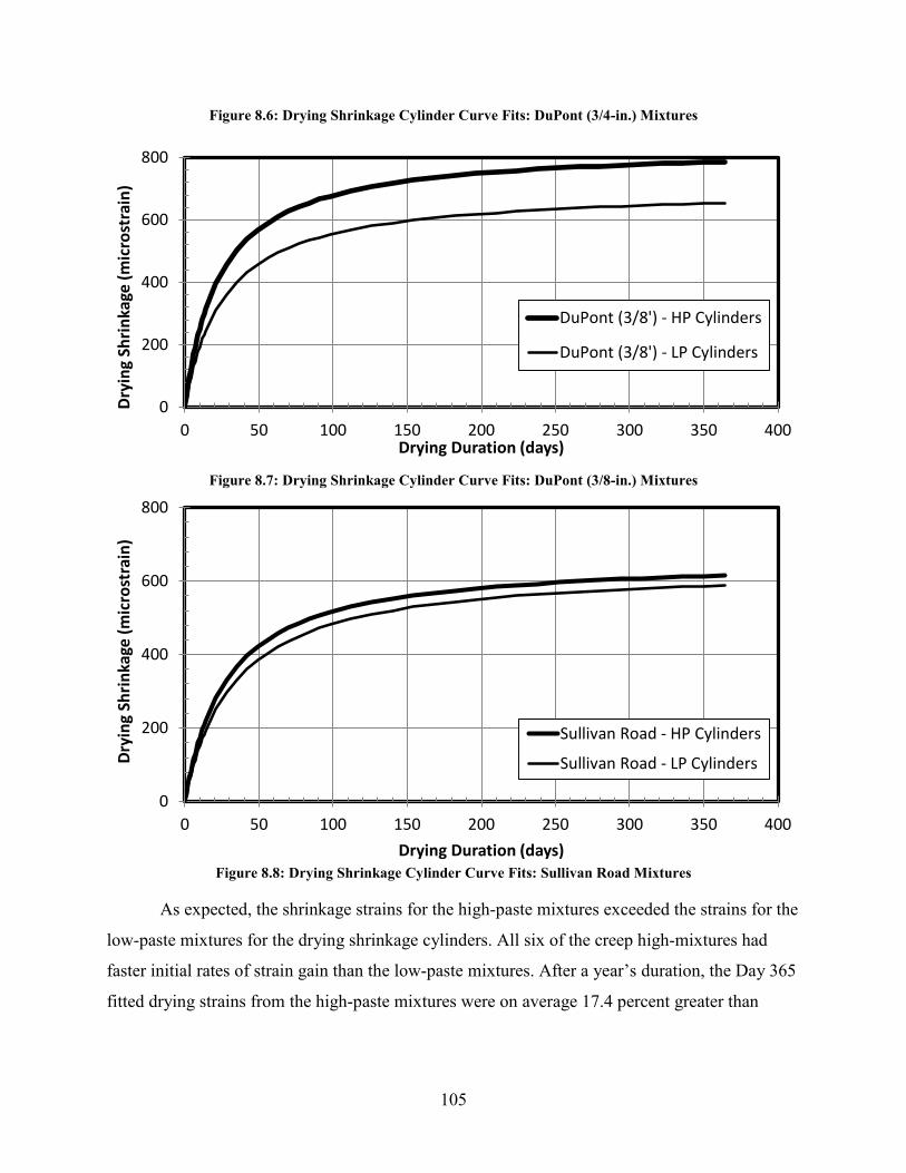
Figure 8.6: Drying Shrinkage Cylinder Curve Fits: DuPont (3/4-in.) Mixtures
Figure 8.7: Drying Shrinkage Cylinder Curve Fits: DuPont (3/8-in.) Mixtures
Figure 8.8: Drying Shrinkage Cylinder Curve Fits: Sullivan Road Mixtures
As expected, the shrinkage strains for the high-paste mixtures exceeded the strains for the
low-paste mixtures for the drying shrinkage cylinders. All six of the creep high-mixtures had
faster initial rates of strain gain than the low-paste mixtures. After a year’s duration, the Day 365
fitted drying strains from the high-paste mixtures were on average 17.4 percent greater than
0
200
400
600
800
0 50 100 150 200 250 300 350 400
Dryi
ng S
hrin
kage
(mic
rost
rain
)
Drying Duration (days)
DuPont (3/8') - HP Cylinders
DuPont (3/8') - LP Cylinders
0
200
400
600
800
0 50 100 150 200 250 300 350 400
Dryi
ng S
hrin
kage
(mic
rost
rain
)
Drying Duration (days)
Sullivan Road - HP Cylinders
Sullivan Road - LP Cylinders
105

those of the low-paste mixtures. This comparison shows a consistent effect of the paste content
on the drying shrinkage strains. This effect is not accounted for by the AASHTO specifications
(5.4.2.3.3-1), which does not consider mixture proportions.
8.2.4 Creep Strains
The creep strains for each concrete mixture were fit to Equation 8.2. The optimized
coefficients and fitted Day 365 strains for each creep mixture are listed in Table 8.9. The creep
rigs had a targeted stress of 35 percent of the Day 14 compressive strength; therefore, the
loadings for each rig were different. Since the creep rigs did not have similar loadings, there was
no comparison of the measured creep strain data.
Table 8.9: Optimized Fitted Creep Curve Coefficients: All Mixtures
𝐟𝐟�̅�𝟒 (psi)
𝐭𝟓𝟎 (Days)
𝛆𝐔𝐥𝐭 (microstrain)
𝐅𝐢𝐭𝐭𝐞𝐝 𝛆𝟑𝟔𝟔𝟓 (microstrain) 𝛆𝟐𝟖 / 𝛆𝟑𝟔𝟔𝟓
DuPont (3/4") - HP 4,990 26.9 850 790 0.55 DuPont (3/4") - LP 3,710 21.7 730 690 0.62 DuPont (3/8") - HP 4,770 30.4 850 780 0.53 DuPont (3/8") - LP 5,170 22.0 980 920 0.60 Sullivan Road - HP 4,650 15.4 940 900 0.72 Sullivan Road - LP 4,410 17.6 790 750 0.70
8.2.5 Specific Creep
The specific creep was determined for each mixture by dividing the creep strains by the
applied stress (in psi), which was determined by the measured elastic strain values. The specific
creep optimized coefficients are listed in Table 8.10. The specific creep curves are plotted for all
of the creep mixtures in Figure 8.9.
106

Table 8.10: Optimized Coefficients for Specific Creep: All Mixtures
𝐭𝟓𝟎
(Days) Day 365 𝛆𝟐𝟖 / 𝛆𝟑𝟔𝟔𝟓
DuPont (3/4") - HP 27.0 0.43 0.55 DuPont (3/4") - LP 21.9 0.49 0.60 DuPont (3/8") - HP 29.9 0.45 0.52 DuPont (3/8") - LP 22.1 0.48 0.59 Sullivan Road - HP 15.4 0.53 0.68 Sullivan Road - LP 17.5 0.48 0.65
Figure 8.9: Specific Creep Fitted Curves: All Creep Mixtures
The three low-paste mixtures had similar specific creep curves (average difference of 2.4
percent). The DuPont (3/4-in. and 3/8-in.) high-paste mixtures had similar curves (average
difference of 1.5 percent) that were approximately 16 percent smaller than the low-paste specific
creep values. The Day 365 specific creep strains ranged from 0.43 to 0.53, with an average of
0.48 and a coefficient of variation of 7.5 percent. The ratio of Day 28 to Day 365 of the
normalized strains ranged from 0.52 to 0.68, with an average ratio of 0.60 and a coefficient of
variation of 9.9 percent. Figure 8.9 shows that variations in aggregate size had little effect on the
0.0
0.1
0.2
0.3
0.4
0.5
0.6
0 50 100 150 200 250 300 350 400
Spec
ific C
reep
(mic
rost
rain
/ ps
i)
Creep Duration (days)
DuPont (3/4") - HP, Specific CreepDuPont (3/4") - LP, Specific CreepDuPont (3/8") - HP, Specific CreepDuPont (3/8") - LP, Specific CreepSullivan Road - HP, Specific CreepSullivan Road - LP, Specific Creep
107
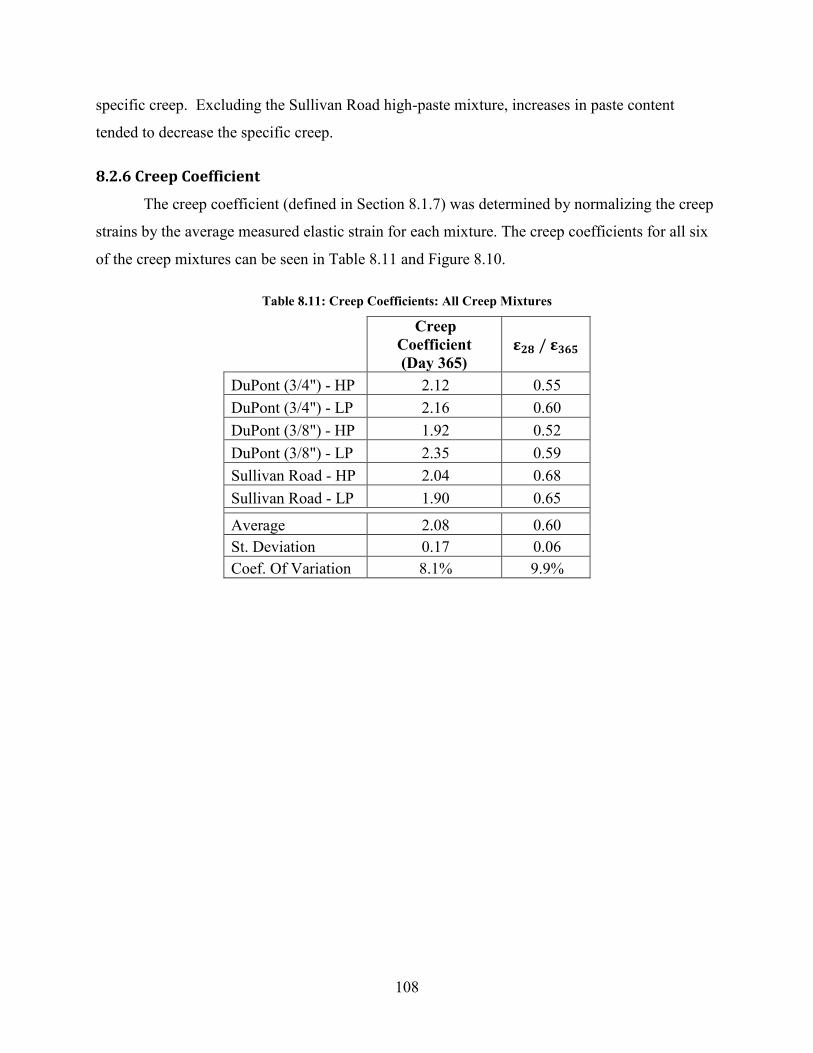
specific creep. Excluding the Sullivan Road high-paste mixture, increases in paste content
tended to decrease the specific creep.
8.2.6 Creep Coefficient
The creep coefficient (defined in Section 8.1.7) was determined by normalizing the creep
strains by the average measured elastic strain for each mixture. The creep coefficients for all six
of the creep mixtures can be seen in Table 8.11 and Figure 8.10.
Table 8.11: Creep Coefficients: All Creep Mixtures
Creep Coefficient (Day 365)
𝛆𝟐𝟖 / 𝛆𝟑𝟔𝟔𝟓
DuPont (3/4") - HP 2.12 0.55 DuPont (3/4") - LP 2.16 0.60 DuPont (3/8") - HP 1.92 0.52 DuPont (3/8") - LP 2.35 0.59 Sullivan Road - HP 2.04 0.68 Sullivan Road - LP 1.90 0.65
Average 2.08 0.60 St. Deviation 0.17 0.06 Coef. Of Variation 8.1% 9.9%
108

Figure 8.10: Creep Coefficient: All Creep Mixtures
The plot shows that all six of the fitted curves for the laboratory mixtures were similar.
The fitted Day 365 coefficients ranged from 1.90 to 2.35, with an average coefficient of 2.08.
The ratio of Day 28 to Day 365 for the coefficients ranged from 0.55 to 0.68, with an average
ratio of 0.60. The creep coefficient after a year’s loading duration had a coefficient of variation
that was approximately 8 percent for six concrete mixtures, despite the variations in compressive
strengths, elastic strains, paste contents, aggregate size, and aggregate type.
The aggregate source appeared to affect the ratio of Day 28 to Day 365 creep
coefficients. The DuPont aggregates (3/4-in. and 3/8-in.) had an average ratio of 0.56, and the
Sullivan Road aggregate had an average ratio of 0.66 (a difference of 14.9 percent). There was
no consistent pattern for the effect of variations in paste content on the creep coefficients.
A comparison of the creep coefficient curves for the laboratory mixtures and the
estimated curve from AASHTO specifications (5.4.2.3.2-1, Equation 2.12) are provided in
Appendix D. The results are consistent with those detailed in Section 8.1.7. Namely, the creep
coefficients at one year were well estimated by the AASHTO specifications. The difference
between the predicted and measured Day 365 creep coefficients ranged from 1.7 percent to 16.2
percent, with an average difference of 8.0 percent. However, the measured creep coefficient
curves and estimated AASHTO creep coefficient curves did not match well for any mixtures at
0.0
0.4
0.8
1.2
1.6
2.0
2.4
0 50 100 150 200 250 300 350 400
Cree
p Co
effic
ient
(mic
rost
rain
/ ks
i)
Creep Duration (days)
DuPont (3/4") - HPDuPont (3/4") - LPDuPont (3/8") - HPDuPont (3/8") - LPSullivan Road - HPSullivan Road - LP
109

early ages. The difference in Day 28 to 365 ratios from the measured and estimated values
ranged from 21.7 percent to 41.2 percent, with an average difference of 31.6 percent. By taking
the aggregate source into account in the AASHTO specifications, it may be possible to improve
the accuracy of the estimated creep coefficients at early ages.
The method of analyzing the creep strain variability, as detailed in Section 8.1.7, was
repeated for all six of the creep mixtures. The method calculated three distinct creep strain values
by dividing an applied stress of 1,600 psi (40 percent of the 4,000 psi design strength) by various
elastic moduli (the measured elastic modulus, the predicted elastic modulus from the Day 14
compressive strength, and the predicted elastic modulus from the design strength of 4,000 psi).
The estimated creep strain curves for each of the elastic strain values and the measured creep
strain curve for each mixture can be seen in Appendix D. The differences from the measured and
estimated creep strain and the average coefficient of variation for each of the AASHTO curves
are listed in Table 8.12 for the creep mixtures.
Table 8.12: Predicted AASHTO Creep Strain Curve Differences: All Mixtures
ε365 Percentage Difference Average Coefficient of Variation
Fitted ε365 Design
Strength
Predicted Elastic
Modulus
Measured Elastic
Modulus
Design Strength
Predicted Elastic
Modulus
Measured Elastic
Modulus DuPont (3/4") - HP 790 28.7% 20.4% 4.0% 18.3% 11.7% 4.7% DuPont (3/4") - LP 690 18.7% 21.7% 4.4% 10.7% 12.6% 6.2% DuPont (3/8") - HP 780 26.2% 19.4% 9.4% 16.7% 11.2% 5.2% DuPont (3/8") - LP 920 20.7% 9.8% 1.5% 11.9% 6.8% 8.7% Sullivan Road - HP 900 11.7% 4.8% 6.9% 8.9% 8.3% 8.2% Sullivan Road - LP 750 20.0% 16.1% 12.6% 11.9% 9.9% 8.6%
Average 810 21.0% 15.4% 6.5% 13.1% 10.1% 6.9%
The results suggest that to improve the accuracy of AASHTO prediction curves, the
measured compressive strength and elastic modulus should be known for each application. If
standardized tests cannot be performed, then the AASHTO specifications for estimating the
elastic modulus (Section 5.4.2.4-1, Equation 2.7) need to be improved.
110

8.3 CREEP CURVE EXTRAPOLATION VARIABILITY
Error was caused by shortening the monitored creep duration. The creep strains for the
DuPont (3/4-in.) high-paste samples at various durations were fit to Equation 8.2 and
extrapolated to a year’s duration. The average percentage difference between the creep strains
monitored for a year and the different durations are listed in Table 8.13. The fitted curves for
each of the different monitored durations are shown in Figure 8.11.
Table 8.13: Percentage Difference from Varying Creep Monitor Durations
Monitored Duration
(days)
Fitted 𝛆𝟑𝟔𝟔𝟓 (percentage difference)
Average Strains (percentage difference)
270 9.4% 7.1% 180 14.2% 11.0% 90 22.8% 18.3% 56 28.9% 23.7% 28 34.6% 28.9%
Figure 8.11: Strain Extrapolation Error: DuPont (3/4-in.) High-Paste
0
100
200
300
400
500
600
700
800
0 50 100 150 200 250 300 350 400
Cree
p St
rain
(mic
rost
rain
)
Load Duration (days)
365 Days270 Days180 Days90 Days56 Days28 Days
111
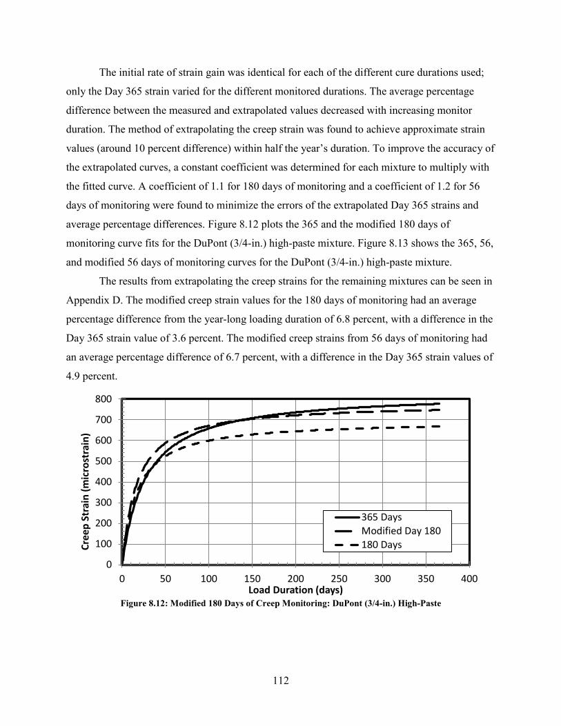
The initial rate of strain gain was identical for each of the different cure durations used;
only the Day 365 strain varied for the different monitored durations. The average percentage
difference between the measured and extrapolated values decreased with increasing monitor
duration. The method of extrapolating the creep strain was found to achieve approximate strain
values (around 10 percent difference) within half the year’s duration. To improve the accuracy of
the extrapolated curves, a constant coefficient was determined for each mixture to multiply with
the fitted curve. A coefficient of 1.1 for 180 days of monitoring and a coefficient of 1.2 for 56
days of monitoring were found to minimize the errors of the extrapolated Day 365 strains and
average percentage differences. Figure 8.12 plots the 365 and the modified 180 days of
monitoring curve fits for the DuPont (3/4-in.) high-paste mixture. Figure 8.13 shows the 365, 56,
and modified 56 days of monitoring curves for the DuPont (3/4-in.) high-paste mixture.
The results from extrapolating the creep strains for the remaining mixtures can be seen in
Appendix D. The modified creep strain values for the 180 days of monitoring had an average
percentage difference from the year-long loading duration of 6.8 percent, with a difference in the
Day 365 strain value of 3.6 percent. The modified creep strains from 56 days of monitoring had
an average percentage difference of 6.7 percent, with a difference in the Day 365 strain values of
4.9 percent.
Figure 8.12: Modified 180 Days of Creep Monitoring: DuPont (3/4-in.) High-Paste
0
100
200
300
400
500
600
700
800
0 50 100 150 200 250 300 350 400
Cree
p St
rain
(mic
rost
rain
)
Load Duration (days)
365 DaysModified Day 180180 Days
112

Figure 8.13: Modified 56 Days of Creep Monitoring: DuPont (3/4-in.) High-Paste
8.4 ANALYSIS OF CREEP RESULTS
Variations in the aggregate type, compressive strength, and paste content significantly
affected the creep strains (Table 8.9).Modeling the specific creep data allowed for a direct
comparison of different creep mixtures by removing the effects of different applied stresses. The
specific creep data showed that the effects of aggregate size and type on specific creep were
minimal, With the exception of the Sullivan Road high-paste mixture, the paste content had a
significant impact (Figure 8.9) on specific creep. For concrete mixtures with lower paste
contents, the specific creep values were larger for the entire loading duration than mixtures with
higher paste contents.
AASHTO specifications (5.4.2.3.2-1, Equation 2.12) estimate year-long creep
coefficients well but under-estimate the initial values (figures 8.4, D.7, D.8, D.9, D.10, and
D.11). This may become a concern for structures that have larger creep deflections at earlier ages
than expected, as predicted by AASHTO specifications, when those deformations are to be
expected. When the creep coefficient is converted into an estimation of the creep strain,
knowledge of the measured compressive strength and elastic modulus from standardized testing
would greatly improve the accuracy of the calculated strain values (Table 8.12).
0
100
200
300
400
500
600
700
800
0 50 100 150 200 250 300 350 400
Cree
p St
rain
(mic
rost
rain
)
Creep Duration (days)
365 DaysModified Day 5656 Days
113
The measured values for the time-dependent strains (drying shrinkage and creep data) can
be modeled well with Equation 8.2 (figures 8.1, D.2, D.3, D.4, D.5, and D.6). The fitted curves
can be used to extrapolate beyond the monitored duration to estimate the future values. This
extrapolation can reduce the required monitoring time for modeling creep strains, and a
coefficient can be used to multiply the fitted curves and improve the accuracy. For monitoring
durations of 180 days, a coefficient of 1.1 consistently improved the extrapolated creep data
(figures 8.12, D.17, D.18, D.19, D.20, and D.21). Monitoring durations of 56 days can be
improved consistently by using a coefficient of 1.2 for extrapolated creep strains (figures 8.13,
D.22, D.23, D.24, D.25, and D.26).
114
Chapter 9: Summary of Findings and Recommendations
This chapter summarizes the finding and recommendations based on the evaluation of
key performance characteristics for (1) twenty-eight laboratory mixtures, consisting of four
mixtures (high strength, low strength, high paste and low paste) for seven aggregate types, and
(2) concrete mixtures sampled from five WSDOT bridge projects.
The compressive strength, tensile strength, elastic modulus, drying shrinkage, and creep
parameters were the key performance characteristics that were considered. In this chapter, a
section is devoted to each characteristic. Within each section, a subsection is devoted to the
effects of the concrete mixture proportions (paste content and water-cementitious ratio) and
coarse aggregate source, to summarize the accuracy of the current relevant specifications, and to
make recommendations.
9.1 COMPRESSIVE STRENGTH
Compressive strengths were measured for the 28 laboratory mixtures at 7, 14, 28 and 56
days. Compressive strengths of the field mixtures were measured at 28 and 56 days.
9.1.1 Findings
For a given concrete age, the compressive strength of a mixture depended mainly on its
water-cementitious ratio and to a lesser extent, on the aggregate source.
• The compressive strength consistently decreased as the water-cementitious ratio
increased, as expected. This effect was observed consistently for the laboratory mixtures
(Figures 4.2 and 4.7) and field mixtures (Figure 4.12).
• The compressive strength did not vary consistently with paste content (Figure 4.8)
• The strength of most (but not all) of the mixtures was insensitive to the aggregate type.
The exceptions to this insensitivity were that the strengths of the high-strength mixtures
were significantly lower for mixtures made with the Rock Island and Santosh aggregates
(Figure 4.6). As a result, compared with other aggregate sources, the Rock Island
aggregate source (and to a lesser extent, the Santosh aggregate source) were less sensitive
to variations in the water-cementitious ratio (Figure 4.7). This insensitivity suggests that
115

it might be challenging to make higher-strength concrete with aggregates from the Rock
Island and Santosh sources.
The rate of strength gain was evaluated by normalizing the compressive strengths at 7
days by the compressive strengths at 28 days.
• The normalized strength at 7 days was consistently higher for the higher-strength mixes
(w/cm = 0.30 for ¾ in. aggregate) than for the low-strength mixes (w/cm = 0.49). This
difference was observed for all aggregate types (Figure 4.8) and for the five field projects
(Table 4.4).
• The normalized strength at 7 days was insensitive to variations in paste content and
aggregate type (Figure 4.10).
9.1.2 Evaluation of Specifications
The time dependence of the compressive strength was modeled well by the ACI 209.2R-
08 specifications (A-17, Equation 2.1), but only if the equation constants were optimized. For
the laboratory and field mixtures, the optimized values of the K1 and K2 constants were 2.4 and
0.90, respectively. In contrast, ACI 209.2R-08 suggests values of K1 and K2 of 4.0 and 0.85,
respectively. The concrete mixtures cast for this research gained strength significantly faster at
early ages than suggested by the specifications. It is likely that variations in cement type and
cement refinement process since the development of the ACI 209.2R-08 equation have led to an
acceleration in the rate of strength gain.
9.1.3 Recommendations
WSDOT should consider estimating early strength gain using parameters that are
representative of current materials used in Washington State. Further testing would be needed to
evaluate the accuracy of Equation 2.1 for estimating compressive strengths for cure durations
beyond fifty-six days.
9.2 TENSILE STRENGTH
Split-tension and flexural-strength tests were performed at 28 and 56 days for the five
WSDOT project field mixtures.
116
9.2.1 Findings
The following conclusions were drawn from the results of split-tension and flexural tests:
• The flexure strengths (figures 5.2 and 5.3) and split-tensile strengths (figures 5.7 and 5.8)
increased with increasing compressive strength, as expected.
• The flexural strength of the mixtures was approximately equal (on average) to 1.58 times
the split-tension strength (figures 5.9 and 5.10). The correlation between the two
strengths was fit well by Equation 5.2, and the results are similar to the correlation
suggested by ASTM STP 169D (Equation 2.6), which has a factor of 1.54.
• The variability of the strengths of the split tension specimens (average variation of 8.3
percent) generally exceeded that of the flexural strength samples (average variation of 4.0
percent).
The effects of paste content and aggregate source could not be evaluated from the data,
because the sample size was too small, and the split-tension strengths of the cylinders varied too
much among nominally identical samples.
9.2.2 Evaluation of Specifications
The AASHTO code specifications for normal-weight concrete (5.4.2.6, Equation 2.2)
greatly underestimated the flexural strengths of the field samples (lower by an average of 33
percent). In contrast, the AASHTO specifications C5.4.2.6 (Equation 2.3), which was
developed for high-strength concrete, over-predicted the field sample flexure strengths (greater
by an average of 13 percent).
Equation 5.1, developed based on the test results, fit the mean flexural strength of the
field mixtures, with an average difference of 8.3 percent. This equation is repeated in Equation
9.1.
σFLEX (psi) = 420 × �fc�3
(ksi) (Equation 9.1)
9.2.3 Recommendations
Split-tension cylinders are easier to handle than flexural beams, so instead of performing
flexure tests, the modulus of rupture can be predicted from split-tension tests using Equation 5.2,
within a typical error of 7.1 percent. Due to the variability of the split-tension results, it is
117

recommended that a minimum of three split-tension samples be cast per test. Alternately, the
flexural strength could be estimated with Equation 9.1.
9.3 ELASTIC MODULUS
The elastic modulus was measured at 7, 14, 28 and 56 days for four mixtures for each of
the seven aggregate sources. The elastic modulus was also measured at 28 and 56 days for the
five sets of field-collected samples.
9.3.1 Findings
The following findings were reached regarding variations in the elastic modulus at a
particular age:
• The elastic modulus consistently decreased with increasing water-to-cementitious ratio
(Figures 6.1, 6.8 and 6.14).
• The elastic modulus consistently increased with increasing compressive strength (Figures
6.2, 6.7 and 6.15)
• The effect of the paste content on the elastic modulus was not consistent. The elastic
modulus increasing paste content for some aggregate sources. For some other aggregate
sources, the higher-paste mixtures had lower elastic moduli (Figure 6.9).
The following findings were reached regarding the rate at which the elastic modulus
increased:
• The rate of stiffness gain (ratio of Day 7 to Day 28 of the elastic moduli) was not affected
by variations in the water-cementitious ratio or aggregate source (Figures 6.12 and 6.18).
For all high-strength and low-strength mixes, as well as the field samples, the elastic
modulus at 7 days was close to 90 percent of the elastic modulus at 28 days.
• The paste content did not consistently affect the rate of stiffness gain (Figures 6.13 and
6.19).
118

9.3.2 Evaluation of Specifications
Regardless of compressive strength, paste content or aggregate source, the elastic moduli
for all the laboratory mixtures exceeded the values predicted by the AASHTO specifications
(5.4.2.4-1, Equation 2.7) by 10.4 percent, on average (figures 6.10 and 6.11).
Surprisingly, this discrepancy was not identified for the field mixtures, even though the
laboratory and field mixtures used similar paste contents and aggregates from the same sources.
The average difference between the measured and calculated elastic moduli for the field mixtures
was only 4.2 percent.
A possible explanation for this difference is that steel molds were used for the laboratory
mixtures, and plastic molds were used for the field mixtures. Alternately, it is possible that
transportation slightly reduced the elastic modulus of the field samples. The cause of the
differences could not be confirmed within the scope of this study.
Equation 2.7 estimated the elastic modulus for higher strength mixtures more accurately
than lower strength mixtures (Figure 6.3). By accounting for the effect of the water-cementitious
ratio and paste content on the elastic modulus in Equation 6.3, the average difference between
the estimated and measured elastic modulus was 6.9 percent, which was slightly better than
AASHTO predictions (AASHTO specifications had an average difference of 7.8 percent).
9.3.3 Recommendations
Further research would be needed to explain the discrepancy between elastic moduli for
the laboratory cast and field-cast mixtures.
9.4 SHRINKAGE
Drying shrinkage specimens (3 in. by 4 in. by 16 in.) were monitored for 365 days for all
four mixes for each of the seven aggregate sources.
9.4.1 Findings
The drying shrinkage strain increased with
• increasing water-to-cementitious ratio (Figure 7.5),
• increasing paste content (Figures 7.6 and 7.9), and
119

• decreasing volume-to-surface ratio (Figures 7.3, 7.10, 7.11 and 7.12), and
• decreasing compressive strength (Figures 7.7 and 7.8)
The correlation between drying shrinkage and compressive strength is likely attributable
to the correlation between compressive strength and water-to-cementitious ratio
With one exception, the shrinkage strains were similar for all of the ¾-in. aggregates
(Figures 7.8 and 7.9). The exception was the Santosh aggregate source for which the four
mixtures had the highest shrinkage strains of all the mixes for each paste content.
9.4.2 Evaluation of Specifications
When the AASHTO specifications (5.4.2.3.3-1, Equation 2.9) were applied based on the
design strength of 4,000 psi), the specifications greatly overestimated the measured time-related
shrinkage stains (by approximately 45 percent, Figure 7.3). The AASHTO drying shrinkage
strain predictions improved when the measured Day 28 compressive strengths were used, but the
predicted and measured strain still differed typically by about 20 percent (Table 7.3).
Two methods were developed to improve predictions of long-term deformations (one
year drying duration). The first method extrapolates long-term deformations from short duration
tests by optimizing the t50 and ϵ Ult. constants with the following equation.
ϵ time = time
(t50 + time) × ϵ Ult. (Equation 9.2)
Testing was performed for a minimum drying period of 56 days, and then increasing the
extrapolated strain values (using Equation 9.2) by 10 percent to estimate the long-term
deformations. This method resulted in average an error of 8.9 percent for the mixtures tested
(Table 7.10).
A second method was developed to predict long-term deformations directly from key
mixture characteristics. Equation 7.2 predicted one-year drying strains to an accuracy of 6.6
percent for the mixtures tested (Table 7.7), and the form of the equation can be seen in Equation
9.3. Further research for specific aggregate sources would vary the optimized values (K1, K2,
and K3), and could improve the accuracy of Equation 7.2 for different locations.
120

ϵ365 = K1 × (PC × W/CM) + K2� fD̅ay 28�K3 (Equation 9.3)
9.4.3 Recommendations
WSDOT should consider the use of alternate methods for establishing the long-term
shrinkage strains for mixtures made with local materials.
9.5 CREEP
Creep tests were conducted for a year for three aggregate sources (DuPont 3/4”, DuPont
Pea Gravel and Sullivan Road) for both low- and high-paste mixes. Each stack of cylinders was
subjected to a concrete compressive load of approximately 35 percent of the day 14 compressive
strength. The total deformations of pairs of cylinders were then attributed to elastic, drying
shrinkage and creep deformations.
9.5.1 Findings
Based on the results of the six creep tests, the following conclusions were drawn.
• The elastic, drying shrinkage and creep strains all varied according to the aggregate type,
compressive strength, and paste content (Tables 8.8 and 8.9).
• The elastic deformations (Table 8.7) and the shrinkage deformations (Figures 8.6, 8.7 and
8.8) measured for the cylinders in the creep rigs were comparable to those expected based
on elastic modulus and beam shrinkage tests.
• The specific creep (ratio of creep strain to applied stress) varied little for the range of
mixtures considered. At day 365, the specific creep ranged from 0.43 to 0.53 (Table
8.10) with an average of 0.48 and a coefficient of variation of 7.2 percent.
• The creep coefficient (ratio of creep strain) was also insensitive to changes in the mixture
properties. At day 365, the creep coefficient ranged from 1.90 to 2.30 (Table 8.11) with
an average of 2.08 and a coefficient of variation of 8.1 percent.
9.5.2 Evaluation of Specifications
The AASHTO specification estimate the long term creep deformations based on specified
values of the creep coefficient. Using design values of the concrete compressive strength, and
121

calculated values of the elastic modulus and creep coefficient, the measured creep strains
consistently exceeded (on average, by 21 percent) the values predicted following the AASHTO
specifications, which suggest values of the elastic modulus and creep coefficient. The average
error reduced to 15.4 percent when the actual compressive strength was included in the
calculation. The error further reduced to 6.5 percent when the measured elastic modulus was
included in the calculation (Figures 8.5, D.12, D.13, D.14, D.15, and D.16).
Therefore, the creep coefficients specific by the AASHTO specifications are consistent
with the measured creep deformations. The errors in the estimates of creep strains appear to
stem mainly from differences between assumed and measured values of the concrete
compressive strength and elastic modulus.
Long-term (one-year) predictions of creep strains can be made based on data from shorter
testing durations. ). For example, based on Equation 8.2, fitted for a loading duration of 56 days,
and then increased the extrapolated one-year predictions by 20 percent resulted in average creep
strain errors of 6.7 percent (Figures 8.13, D.22, D.23, D.24, D.25, and D.26).
9.5.3 Recommendations
Estimates of long-term creep deformations could be best improved by making accurate
estimates of the actual concrete strength (as opposed to specified strength) and estimates of the
actual elastic modulus.
122

Acknowledgments
This study was made possible through the time and effort of the faculty members at the
University of Washington and the employees of the Washington State Department of
Transportation. Special thanks to Ron Lewis, Kim Willoughby, DeWayne Wilson, and Jugesh
Kapur for their support. Yiming Liu of the Materials Testing Laboratory at the University of
Washington helped provide the safety training required to operate all of the equipment for this
research. Lastly, thanks to Spencer Livermore and Bradley Maier for their assistance in casting
laboratory and field concrete samples. Only through the contributions of these individuals was
successful completion of this research possible.
123

Bibliography
2010 Annual Book of ASTM Standards, Concrete and Aggregates, Volume 04.02. Baltimore,
MD: ASTM International, 2010.
AASHTO LRFD Bridge Design Specifications. Washington, DC: American Association of State
Highway and Transportation Officials, 2012.
Building Code Requirements for Structural Concrete (ACI 318-08) and Commentary.
Farmington Hills, MI: American Concrete Institute, 2008.
Guide for Modeling and Calculating Shrinkage and Creep in Hardened Concrete, ACI 209.2R-
08. Farmington Hills, MI: American Concrete Institute, 2008.
Mehta, Kumar and Monteiro, Paulo. Concrete Microstructure, Properties, and Materials, Third
Edition. New York, NY: McGraw-Hill Companies, Inc., 2006.
Neville, A. Properties of Concrete. London, UK: Pitman Publishing LTD., 1975.
Prediction of Creep, Shrinkage, and Temperature Effects in Concrete Structures, ACI 209R-92. .
Farmington Hills, MI: American Concrete Institute, 2008.
Significance of Tests and Properties of Concrete and Concrete-Making Materials, ASTM STP-
169D. Bridgeport, NJ: ASTM International, 2006.
124

125

Appendix A: Compressive Strength Test Results
A.1: SUMMARY OF MEASURED COMPRESSIVE STRENGTHS
The measured compressive strength results from the four test dates are shown in this
section for each laboratory mixture. The compressive strengths from DuPont (3/4-in.) mixture
are excluded in this section, but can be seen in Table 4.1 and Figure 4.1. The following list of
tables and figures detail the measured compressive strengths for laboratory aggregate: Table A.1
and Figure A.1 for DuPont (3/8-in.), Table A.2 and Figure A.2 for Okanogan Valley, Table A.3
and Figure A.3 for Sullivan Road, Table A.4 and Figure A.4 for Pasco, Table A.5 and Figure A.5
for Rock Island, and Table A.6 and Figure A.6 for Santosh mixtures.
Table A.1: Measured Compressive Strengths: DuPont (3/8-in.)
Mixture Paste
Content (%)
Water-Cementitious
Ratio
Day 7 (psi)
Day 14
(psi)
Day 28
(psi)
Day 56 (psi)
High Paste 33.2 0.38 4,310 4,770 5,460 5,630 Low Paste 26.1 0.38 4,440 5,170 5,690 6,250
High Strength 28.2 0.33 4,570 4,950 5,610 5,560 Low Strength 29.3 0.49 2,690 3,390 3,850 4,000
Figure A.1: Compressive Strengths: DuPont (3/8-in.) Mixtures
0
1,000
2,000
3,000
4,000
5,000
6,000
7,000
8,000
0 10 20 30 40 50 60
Com
pres
sive
Str
engt
h (p
si)
Age (days)
High PasteLow PasteHigh StrengthLow Strength
A-1
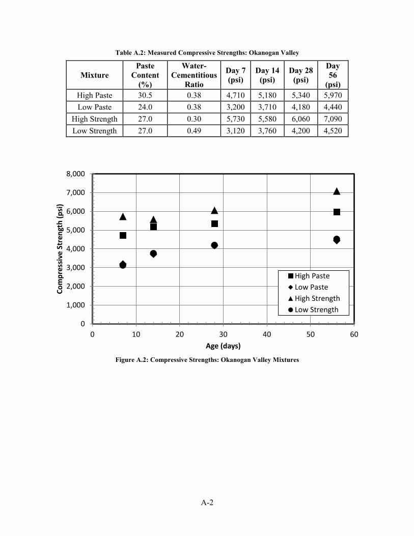
Table A.2: Measured Compressive Strengths: Okanogan Valley
Mixture Paste
Content (%)
Water-Cementitious
Ratio
Day 7 (psi)
Day 14 (psi)
Day 28 (psi)
Day 56
(psi) High Paste 30.5 0.38 4,710 5,180 5,340 5,970 Low Paste 24.0 0.38 3,200 3,710 4,180 4,440
High Strength 27.0 0.30 5,730 5,580 6,060 7,090 Low Strength 27.0 0.49 3,120 3,760 4,200 4,520
Figure A.2: Compressive Strengths: Okanogan Valley Mixtures
0
1,000
2,000
3,000
4,000
5,000
6,000
7,000
8,000
0 10 20 30 40 50 60
Com
pres
sive
Str
engt
h (p
si)
Age (days)
High PasteLow PasteHigh StrengthLow Strength
A-2

Table A.3: Measured Compressive Strengths: Sullivan Road
Mixture Paste
Content (%)
Water-Cementitiou
s Ratio
Day 7 (psi)
Day 14 (psi)
Day 28 (psi)
Day 56 (psi)
High Paste 30.5 0.38 4,080 4,650 4,720 5,260 Low Paste 24.0 0.38 3,950 4,410 4,830 5,370
High Strength 27.0 0.30 5,820 6,370 6,750 7,300 Low Strength 27.0 0.49 2,980 3,490 3,810 4,340
Figure A.3: Compressive Strengths: Sullivan Road Mixtures
0
1,000
2,000
3,000
4,000
5,000
6,000
7,000
8,000
0 10 20 30 40 50 60
Com
pres
sive
Str
engt
h (p
si)
Age (days)
High PasteLow PasteHigh StrengthLow Strength
A-3
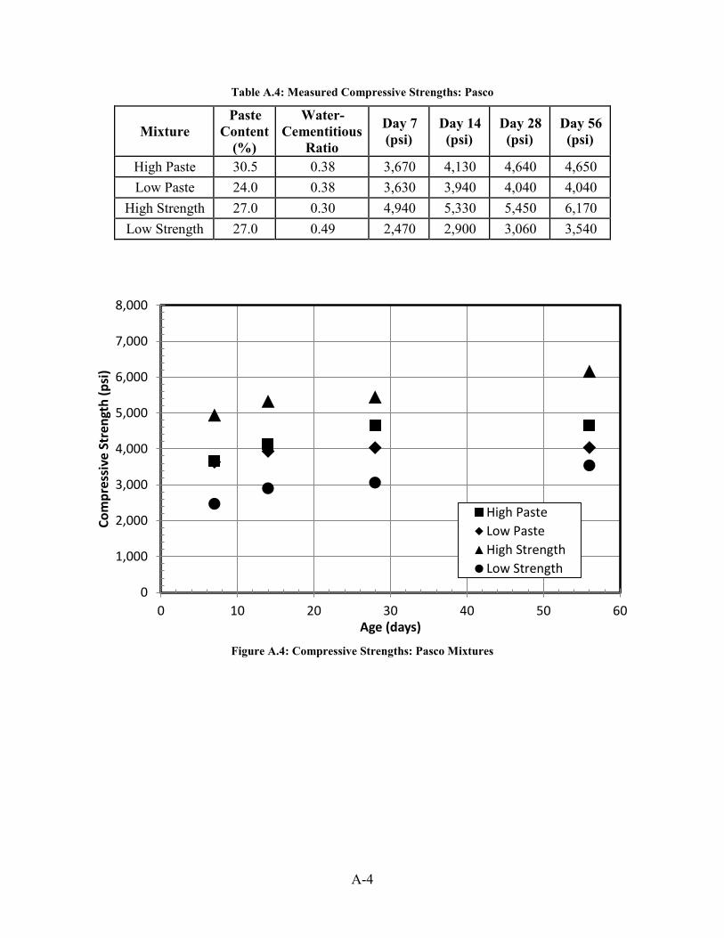
Table A.4: Measured Compressive Strengths: Pasco
Mixture Paste
Content (%)
Water-Cementitious
Ratio
Day 7 (psi)
Day 14 (psi)
Day 28 (psi)
Day 56 (psi)
High Paste 30.5 0.38 3,670 4,130 4,640 4,650 Low Paste 24.0 0.38 3,630 3,940 4,040 4,040
High Strength 27.0 0.30 4,940 5,330 5,450 6,170 Low Strength 27.0 0.49 2,470 2,900 3,060 3,540
Figure A.4: Compressive Strengths: Pasco Mixtures
0
1,000
2,000
3,000
4,000
5,000
6,000
7,000
8,000
0 10 20 30 40 50 60
Com
pres
sive
Str
engt
h (p
si)
Age (days)
High PasteLow PasteHigh StrengthLow Strength
A-4
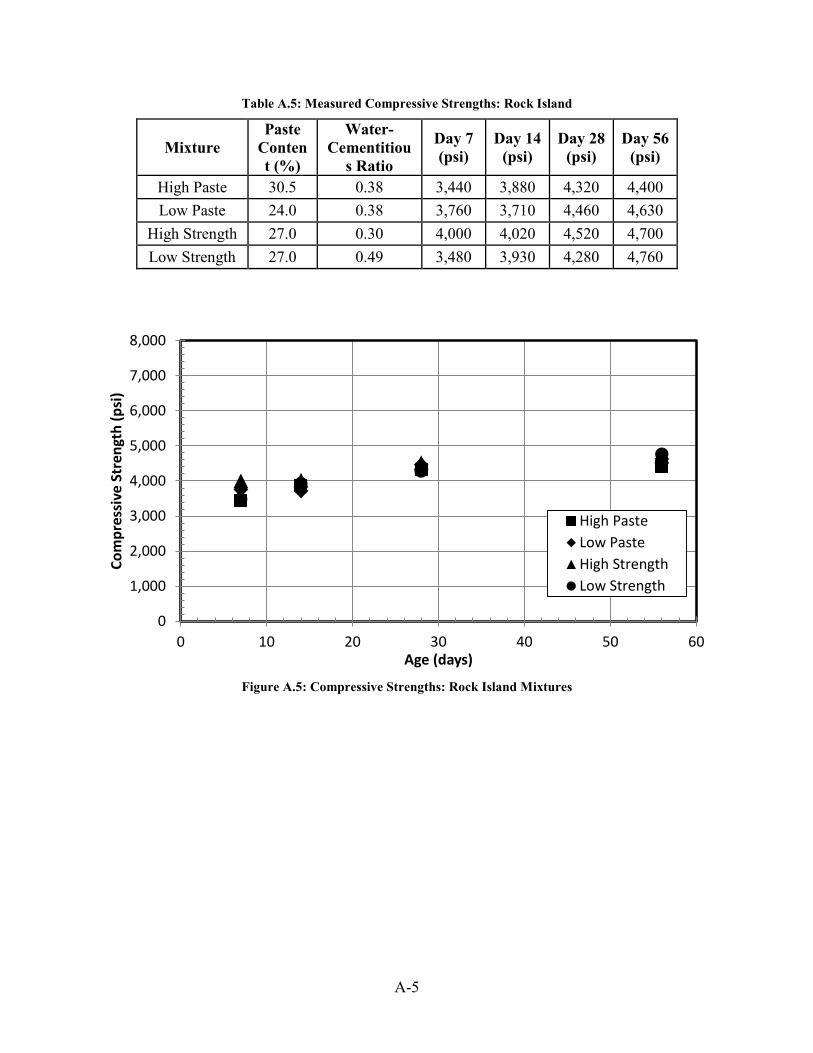
Table A.5: Measured Compressive Strengths: Rock Island
Mixture Paste
Content (%)
Water-Cementitiou
s Ratio
Day 7 (psi)
Day 14 (psi)
Day 28 (psi)
Day 56 (psi)
High Paste 30.5 0.38 3,440 3,880 4,320 4,400 Low Paste 24.0 0.38 3,760 3,710 4,460 4,630
High Strength 27.0 0.30 4,000 4,020 4,520 4,700 Low Strength 27.0 0.49 3,480 3,930 4,280 4,760
Figure A.5: Compressive Strengths: Rock Island Mixtures
0
1,000
2,000
3,000
4,000
5,000
6,000
7,000
8,000
0 10 20 30 40 50 60
Com
pres
sive
Str
engt
h (p
si)
Age (days)
High PasteLow PasteHigh StrengthLow Strength
A-5

Table A.6: Measured Compressive Strengths: Santosh
Mixture Paste
Content (%)
Water-Cementitious
Ratio
Day 7 (psi)
Day 14 (psi)
Day 28 (psi)
Day 56 (psi)
High Paste 30.5 0.38 2,690 3,040 3,170 3,380 Low Paste 24.0 0.38 2,680 2,920 3,190 3,580
High Strength 27.0 0.30 4,160 4,350 4,630 4,890 Low Strength 27.0 0.49 2,470 2,510 3,340 3,640
Figure A.6: Compressive Strengths: Santosh Mixtures
The measured Day 28 compressive strengths were plotted against the water-cementitious
ratios for each laboratory aggregate sources. The Day 28 strengths versus the water-cementitious
ratios of the DuPont (3/4-in.) mixtures are excluded from this section, but can be seen in Figure
4.2. The following list of figures show the Day 28 strengths against the water-cementitious ratios
for each of the four laboratory mixtures: Figure A.7 for DuPont (3/8-in.), Figure A.8 for
Okanogan Valley, Figure A.9 for Sullivan Road, Figure A.10 for Pasco, Figure A.11 for Rock
Island, and Figure A.12 for Santosh mixtures.
0
1,000
2,000
3,000
4,000
5,000
6,000
7,000
8,000
0 10 20 30 40 50 60
Com
pres
sive
Str
engt
h (p
si)
Age (days)
High PasteLow PasteHigh StrengthLow Strength
A-6
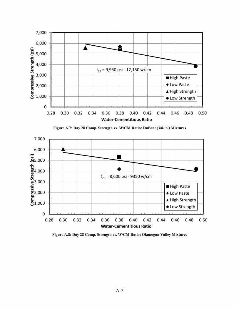
Figure A.7: Day 28 Comp. Strength vs. W/CM Ratio: DuPont (3/8-in.) Mixtures
Figure A.8: Day 28 Comp. Strength vs. W/CM Ratio: Okanogan Valley Mixtures
f28 = 9,950 psi - 12,150 w/cm
0
1,000
2,000
3,000
4,000
5,000
6,000
7,000
0.28 0.30 0.32 0.34 0.36 0.38 0.40 0.42 0.44 0.46 0.48 0.50
Com
pres
sive
Str
engt
h (p
si)
Water-Cementitious Ratio
High PasteLow PasteHigh StrengthLow Strength
f28 = 8,600 psi - 9350 w/cm
0
1,000
2,000
3,000
4,000
5,000
6,000
7,000
0.28 0.30 0.32 0.34 0.36 0.38 0.40 0.42 0.44 0.46 0.48 0.50
Com
pres
sive
Str
engt
h (p
si)
Water-Cementitious Ratio
High PasteLow PasteHigh StrengthLow Strength
A-7

Figure A.9: Day 28 Comp. Strength vs. W/CM Ratio: Sullivan Road Mixtures
Figure A.10: Day 28 Comp. Strength vs. W/CM Ratio: Pasco Mixtures
f28 = 10,800 - 14,850 w/cm
0
1,000
2,000
3,000
4,000
5,000
6,000
7,000
0.28 0.30 0.32 0.34 0.36 0.38 0.40 0.42 0.44 0.46 0.48 0.50
Com
pres
sive
Str
engt
h (p
si)
Water-Cementitious Ratio
High PasteLow PasteHigh StrengthLow Strength
f28 = 9,150 psi - 12,500 w/cm
0
1,000
2,000
3,000
4,000
5,000
6,000
7,000
0.28 0.30 0.32 0.34 0.36 0.38 0.40 0.42 0.44 0.46 0.48 0.50
Com
pres
sive
Str
engt
h (p
si)
Water-Cementitious Ratio
High PasteLow PasteHigh StrengthLow Strength
A-8
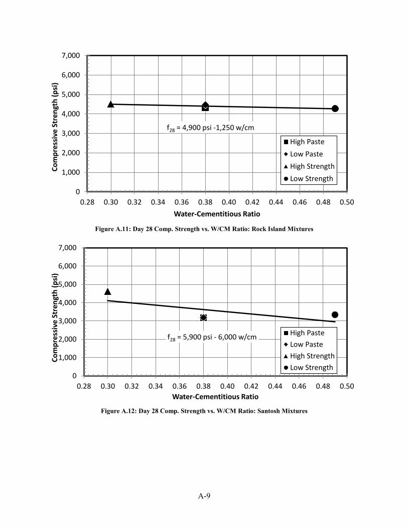
Figure A.11: Day 28 Comp. Strength vs. W/CM Ratio: Rock Island Mixtures
Figure A.12: Day 28 Comp. Strength vs. W/CM Ratio: Santosh Mixtures
f28 = 4,900 psi -1,250 w/cm
0
1,000
2,000
3,000
4,000
5,000
6,000
7,000
0.28 0.30 0.32 0.34 0.36 0.38 0.40 0.42 0.44 0.46 0.48 0.50
Com
pres
sive
Str
engt
h (p
si)
Water-Cementitious Ratio
High PasteLow PasteHigh StrengthLow Strength
f28 = 5,900 psi - 6,000 w/cm
0
1,000
2,000
3,000
4,000
5,000
6,000
7,000
0.28 0.30 0.32 0.34 0.36 0.38 0.40 0.42 0.44 0.46 0.48 0.50
Com
pres
sive
Str
engt
h (p
si)
Water-Cementitious Ratio
High PasteLow PasteHigh StrengthLow Strength
A-9

A.2: RATE OF STRENGTH GAIN
The compressive strengths for each mixture were normalized by the Day 28 strength and
fit to Equation 2.1. The optimized K1 and K2 values are listed in Table A.7 for all of the
laboratory mixtures, with the exclusion of the DuPont (3/4-in.) mixtures. The fitted curves of the
four laboratory mixtures (high and low paste and high and low strength) are shown for each
laboratory aggregate source. The curves from DuPont (3/4-in.) mixture are excluded in this
section, but can be seen in Figure 4.4. The following list of figures shows the fitted curves for
each aggregate source: Figure A.13 for DuPont (3/8-in.), Figure A.14 for Okanogan Valley,
Figure A.15 for Sullivan Road, Figure A.16 for Pasco, Figure A.17 for Rock Island, and Figure
A.18 for Santosh mixtures.
Figure A.13: Rate of Strength Gain Fitted Curves: DuPont (3/8-in.) Mixtures
0.0
0.2
0.4
0.6
0.8
1.0
1.2
0 10 20 30 40 50 60
Nor
mal
ized
Stre
ngth
(Rat
io o
f Day
28)
Time (days)
High PasteLow PasteHigh StrengthLow Strength
A-10
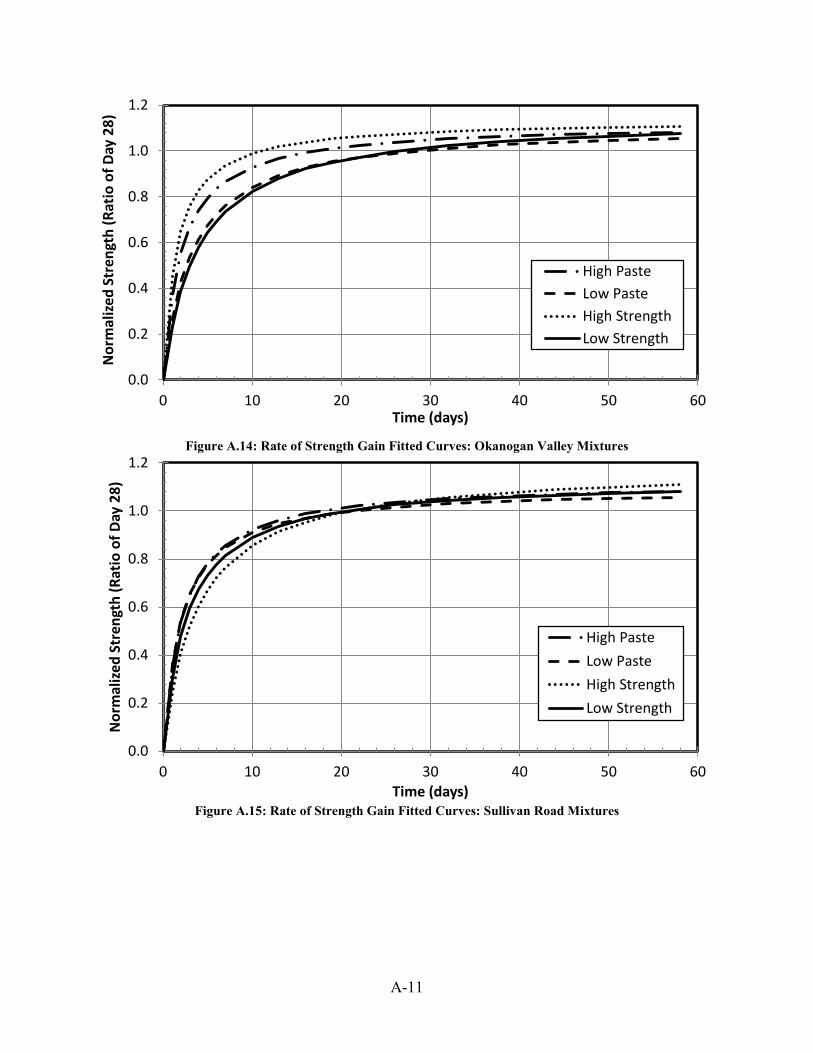
Figure A.14: Rate of Strength Gain Fitted Curves: Okanogan Valley Mixtures
Figure A.15: Rate of Strength Gain Fitted Curves: Sullivan Road Mixtures
0.0
0.2
0.4
0.6
0.8
1.0
1.2
0 10 20 30 40 50 60
Nor
mal
ized
Stre
ngth
(Rat
io o
f Day
28)
Time (days)
High PasteLow PasteHigh StrengthLow Strength
0.0
0.2
0.4
0.6
0.8
1.0
1.2
0 10 20 30 40 50 60
Nor
mal
ized
Stre
ngth
(Rat
io o
f Day
28)
Time (days)
High PasteLow PasteHigh StrengthLow Strength
A-11
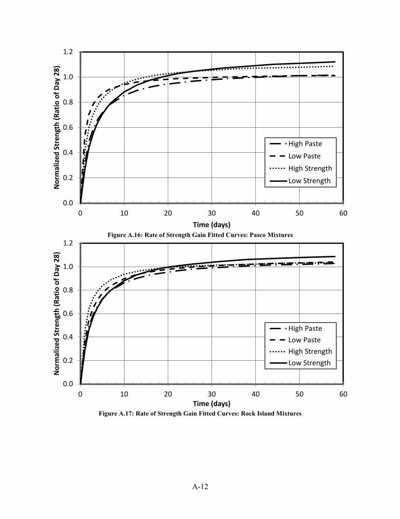
Figure A.16: Rate of Strength Gain Fitted Curves: Pasco Mixtures
Figure A.17: Rate of Strength Gain Fitted Curves: Rock Island Mixtures
0.0
0.2
0.4
0.6
0.8
1.0
1.2
0 10 20 30 40 50 60
Nor
mal
ized
Stre
ngth
(Rat
io o
f Day
28)
Time (days)
High PasteLow PasteHigh StrengthLow Strength
0.0
0.2
0.4
0.6
0.8
1.0
1.2
0 10 20 30 40 50 60
Nor
mal
ized
Stre
ngth
(Rat
io o
f Day
28)
Time (days)
High PasteLow PasteHigh StrengthLow Strength
A-12

Figure A.18: Rate of Strength Gain Fitted Curves: Santosh Mixtures
0.0
0.2
0.4
0.6
0.8
1.0
1.2
0 10 20 30 40 50 60
Nor
mal
ized
Stre
ngth
(Rat
io o
f Day
28)
Time (days)
High PasteLow PasteHigh StrengthLow Strength
A-13

A-14
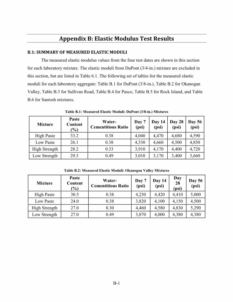
Appendix B: Elastic Modulus Test Results
B.1: SUMMARY OF MEASURED ELASTIC MODULI
The measured elastic modulus values from the four test dates are shown in this section
for each laboratory mixture. The elastic moduli from DuPont (3/4-in.) mixture are excluded in
this section, but are listed in Table 6.1. The following set of tables list the measured elastic
moduli for each laboratory aggregate: Table B.1 for DuPont (3/8-in.), Table B.2 for Okanogan
Valley, Table B.3 for Sullivan Road, Table B.4 for Pasco, Table B.5 for Rock Island, and Table
B.6 for Santosh mixtures.
Table B.1: Measured Elastic Moduli: DuPont (3/8-in.) Mixtures
Mixture Paste
Content (%)
Water-Cementitious Ratio
Day 7 (psi)
Day 14 (psi)
Day 28 (psi)
Day 56 (psi)
High Paste 33.2 0.38 4,040 4,470 4,680 4,590 Low Paste 26.1 0.38 4,530 4,660 4,500 4,850
High Strength 28.2 0.33 3,910 4,170 4,400 4,720 Low Strength 29.3 0.49 3,010 3,170 3,400 3,660
Table B.2: Measured Elastic Moduli: Okanogan Valley Mixtures
Mixture Paste
Content (%)
Water-Cementitious Ratio
Day 7 (psi)
Day 14 (psi)
Day 28
(psi)
Day 56 (psi)
High Paste 30.5 0.38 4,230 4,420 4,410 5,000 Low Paste 24.0 0.38 3,820 4,100 4,150 4,500
High Strength 27.0 0.30 4,460 4,580 4,830 5,290 Low Strength 27.0 0.49 3,870 4,000 4,380 4,380
B-1

Table B.3: Measured Elastic Moduli: Sullivan Road Mixtures
Mixture Paste
Content (%)
Water-Cementitious Ratio
Day 7 (psi)
Day 14 (psi)
Day 28
(psi)
Day 56 (psi)
High Paste 30.5 0.38 3,620 3,830 4,040 4,300 Low Paste 24.0 0.38 3,760 3,980 4,000 4,360
High Strength 27.0 0.30 4,790 5,090 5,250 5,570 Low Strength 27.0 0.49 3,670 3,710 4,180 4,230
Table B.4: Measured Elastic Moduli: Pasco Mixtures
Mixture Paste
Content (%)
Water-Cementitious Ratio
Day 7 (psi)
Day 14 (psi)
Day 28
(psi)
Day 56 (psi)
High Paste 30.5 0.38 3,810 3,900 4,050 4,310 Low Paste 24.0 0.38 3,610 4,090 4,280 4,600
High Strength 27.0 0.30 4,510 4,840 4,950 4,930 Low Strength 27.0 0.49 3,310 3,640 3,590 3,760
Table B.5: Measured Elastic Moduli: Rock Island Mixtures
Mixture Paste
Content (%)
Water-Cementitious Ratio
Day 7 (psi)
Day 14 (psi)
Day 28
(psi)
Day 56 (psi)
High Paste 30.5 0.38 3,100 3,660 3,860 3,990 Low Paste 24.0 0.38 3,710 3,670 4,020 4,240
High Strength 27.0 0.30 3,560 3,820 3,980 4,140 Low Strength 27.0 0.49 3,480 3,350 4,130 4,340
Table B.6: Measured Elastic Moduli: Santosh Mixtures
Mixture Paste
Content (%)
Water-Cementitious Ratio
Day 7 (psi)
Day 14 (psi)
Day 28
(psi)
Day 56 (psi)
High Paste 30.5 0.38 3,200 3,350 3,660 3,760 Low Paste 24.0 0.38 3,390 3,480 3,840 3,880
High Strength 27.0 0.30 3,870 4,000 4,230 4,350 Low Strength 27.0 0.49 3,350 3,410 3,760 3,950
B-2

B.2: DAY 28 ELASTIC MODULI VS. WATER-CEMENTITIOUS RATIOS
The effect of the water-cementitious ratio on the elastic modulus for each laboratory
mixture is shown in the follow set of figures. The results of the elastic moduli verses the water-
cementitious ratios from DuPont (3/4-in.) mixture are excluded in this section, but are shown in
Figure 6.1. The following figures show the measured Day 28 elastic moduli against the water-
cementitious ratios for each laboratory mixture: Figure B.1 for DuPont (3/8-in.), Figure B.2 for
Okanogan Valley, Figure B.3 for Sullivan Road, Figure B.4 for Pasco, Figure B.5 for Rock
Island, and Figure B.6 for Santosh mixtures.
Figure B.1: Day 28 Elastic Modulus vs. W/CM Ratio: DuPont (3/8-in.) Mixtures
0
1,000
2,000
3,000
4,000
5,000
6,000
7,000
0.28 0.30 0.32 0.34 0.36 0.38 0.40 0.42 0.44 0.46 0.48 0.50
Elas
tic M
odul
us (k
si)
Water-to-Cementitious Ratio
High Paste
Low Paste
High Strength
Low Strength
E28 Day = 7,150 ksi - 7,350 w/cm
B-3

Figure B.2: Day 28 Elastic Modulus vs. W/CM Ratio: Okanogan Valley Mixtures
Figure B.3: Day 28 Elastic Modulus vs. W/CM Ratio: Sullivan Road Mixtures
0
1,000
2,000
3,000
4,000
5,000
6,000
7,000
0.28 0.3 0.32 0.34 0.36 0.38 0.4 0.42 0.44 0.46 0.48 0.5
Elas
tic M
odul
us (k
si)
Water-to-Cementitious Ratio
High Paste
Low Paste
High Strength
Low Strength
E28 Day = 5,250 ksi - 2,050 w/cm
0
1,000
2,000
3,000
4,000
5,000
6,000
7,000
0.28 0.30 0.32 0.34 0.36 0.38 0.40 0.42 0.44 0.46 0.48 0.50
Elas
tic M
odul
us (k
si)
Water-to-Cementitious Ratio
High Paste
Low Paste
High Strength
Low Strength
E28 Day = 6,300 ksi - 5,000 w/cm
B-4
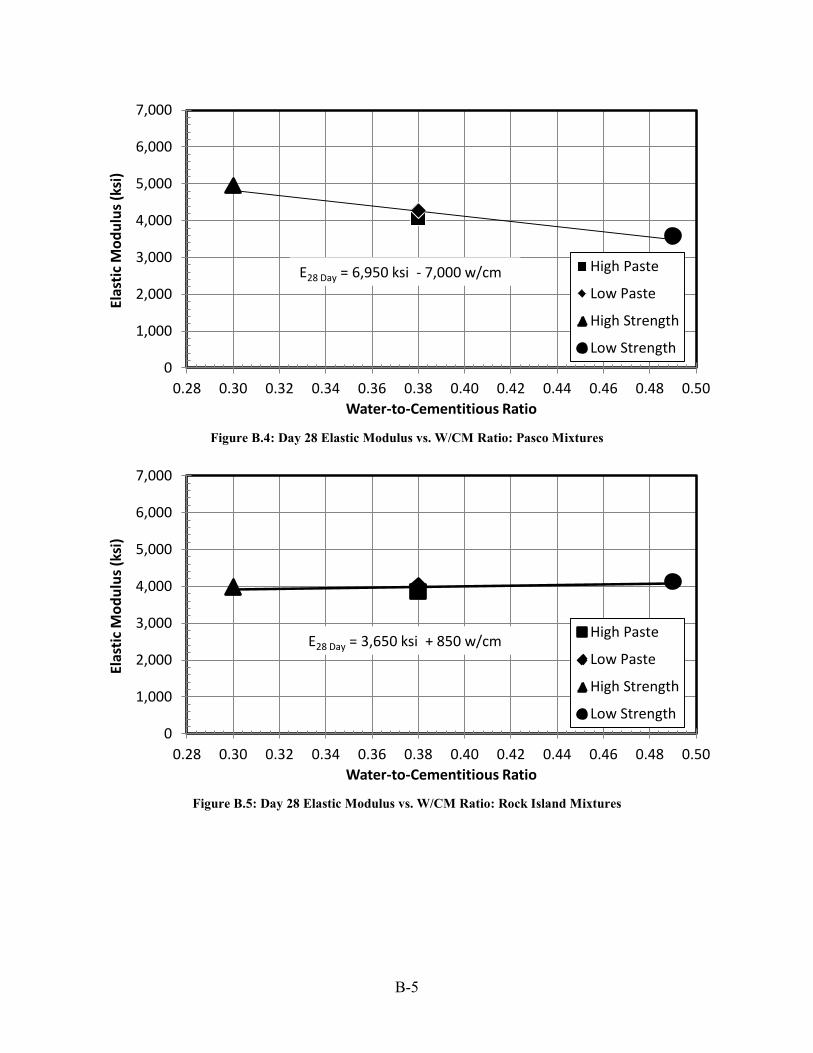
Figure B.4: Day 28 Elastic Modulus vs. W/CM Ratio: Pasco Mixtures
Figure B.5: Day 28 Elastic Modulus vs. W/CM Ratio: Rock Island Mixtures
0
1,000
2,000
3,000
4,000
5,000
6,000
7,000
0.28 0.30 0.32 0.34 0.36 0.38 0.40 0.42 0.44 0.46 0.48 0.50
Elas
tic M
odul
us (k
si)
Water-to-Cementitious Ratio
High Paste
Low Paste
High Strength
Low Strength
E28 Day = 6,950 ksi - 7,000 w/cm
0
1,000
2,000
3,000
4,000
5,000
6,000
7,000
0.28 0.30 0.32 0.34 0.36 0.38 0.40 0.42 0.44 0.46 0.48 0.50
Elas
tic M
odul
us (k
si)
Water-to-Cementitious Ratio
High Paste
Low Paste
High Strength
Low Strength
E28 Day = 3,650 ksi + 850 w/cm
B-5
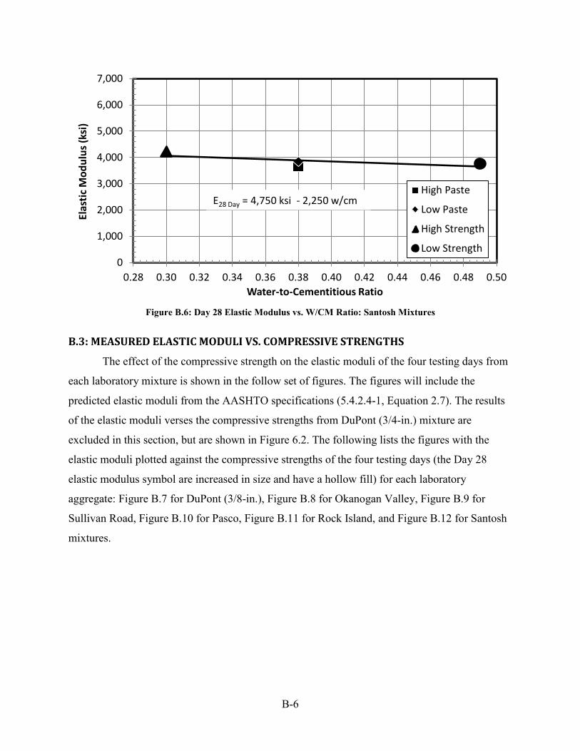
Figure B.6: Day 28 Elastic Modulus vs. W/CM Ratio: Santosh Mixtures
B.3: MEASURED ELASTIC MODULI VS. COMPRESSIVE STRENGTHS
The effect of the compressive strength on the elastic moduli of the four testing days from
each laboratory mixture is shown in the follow set of figures. The figures will include the
predicted elastic moduli from the AASHTO specifications (5.4.2.4-1, Equation 2.7). The results
of the elastic moduli verses the compressive strengths from DuPont (3/4-in.) mixture are
excluded in this section, but are shown in Figure 6.2. The following lists the figures with the
elastic moduli plotted against the compressive strengths of the four testing days (the Day 28
elastic modulus symbol are increased in size and have a hollow fill) for each laboratory
aggregate: Figure B.7 for DuPont (3/8-in.), Figure B.8 for Okanogan Valley, Figure B.9 for
Sullivan Road, Figure B.10 for Pasco, Figure B.11 for Rock Island, and Figure B.12 for Santosh
mixtures.
0
1,000
2,000
3,000
4,000
5,000
6,000
7,000
0.28 0.30 0.32 0.34 0.36 0.38 0.40 0.42 0.44 0.46 0.48 0.50
Elas
tic M
odul
us (k
si)
Water-to-Cementitious Ratio
High Paste
Low Paste
High Strength
Low Strength
E28 Day = 4,750 ksi - 2,250 w/cm
B-6

Figure B.7: Elastic Modulus vs. Compressive Strength: DuPont (3/8-in.) Mixtures
Figure B.8: Elastic Modulus vs. Compressive Strength: Okanogan Valley Mixtures
2,500
3,000
3,500
4,000
4,500
5,000
5,500
6,000
2,500 3,000 3,500 4,000 4,500 5,000 5,500 6,000 6,500 7,000 7,500 8,000
Elas
tic M
odul
us (k
si)
Compressive Strength (psi)
High PasteLow PasteHigh StrengthLow StrengthAASHTO Curve
2,500
3,000
3,500
4,000
4,500
5,000
5,500
6,000
2,500 3,000 3,500 4,000 4,500 5,000 5,500 6,000 6,500 7,000 7,500 8,000
Elas
tic M
odul
us (k
si)
Compressive Strength (psi)
High PasteLow PasteHigh StrengthLow StrengthAASHTO Curve
B-7
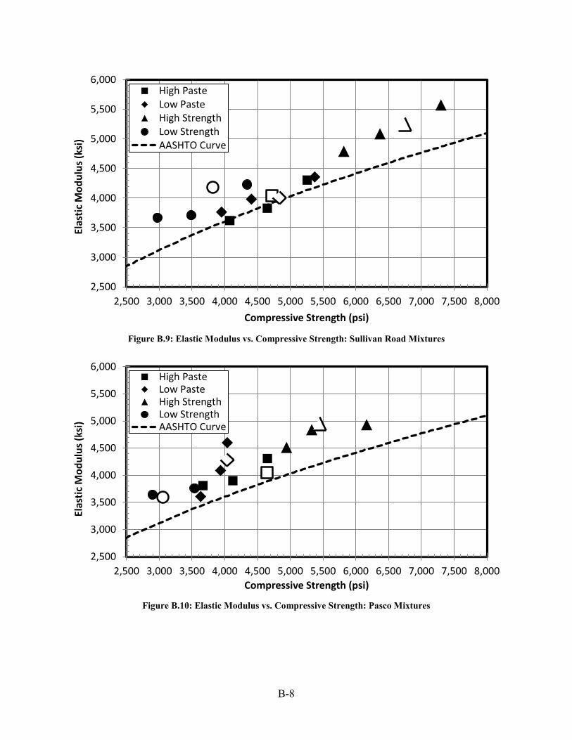
Figure B.9: Elastic Modulus vs. Compressive Strength: Sullivan Road Mixtures
Figure B.10: Elastic Modulus vs. Compressive Strength: Pasco Mixtures
2,500
3,000
3,500
4,000
4,500
5,000
5,500
6,000
2,500 3,000 3,500 4,000 4,500 5,000 5,500 6,000 6,500 7,000 7,500 8,000
Elas
tic M
odul
us (k
si)
Compressive Strength (psi)
High PasteLow PasteHigh StrengthLow StrengthAASHTO Curve
2,500
3,000
3,500
4,000
4,500
5,000
5,500
6,000
2,500 3,000 3,500 4,000 4,500 5,000 5,500 6,000 6,500 7,000 7,500 8,000
Elas
tic M
odul
us (k
si)
Compressive Strength (psi)
High PasteLow PasteHigh StrengthLow StrengthAASHTO Curve
B-8

Figure B.11: Elastic Modulus vs. Compressive Strength: Rock Island Mixtures
Figure B.12: Elastic Modulus vs. Compressive Strength: Santosh Mixtures
2,500
3,000
3,500
4,000
4,500
5,000
5,500
6,000
2,500 3,000 3,500 4,000 4,500 5,000 5,500 6,000 6,500 7,000 7,500 8,000
Elas
tic M
odul
us (k
si)
Compressive Strength (psi)
High PasteLow PasteHigh StrengthLow StrengthAASHTO Curve
2,500
3,000
3,500
4,000
4,500
5,000
5,500
6,000
2,500 3,000 3,500 4,000 4,500 5,000 5,500 6,000 6,500 7,000 7,500 8,000
Elas
tic M
odul
us (k
si)
Compressive Strength (psi)
High PasteLow PasteHigh StrengthLow StrengthAASHTO Curve
B-9

B.4: RATE OF STIFFNESS GAIN
The elastic moduli from the four testing dates were normalized by dividing by the Day 28
elastic modulus for each laboratory mixture. The normalized data was fit to Equation 6.2. The
fitted curves for the elastic moduli from DuPont (3/4-in.) mixture are excluded in this section,
but are shown in Figure 6.6. The optimized values and curve fits of the elastic moduli are listed
in the following tables and figures for each laboratory aggregate: Table B.7 and Figure B.13 for
DuPont (3/8-in.), Table B.8 and Figure B.14 for Okanogan Valley, Table B.9 and Figure B.15
for Sullivan Road, Table B.10 and Figure B.16 for Pasco, Table B.11 and Figure B.17 for Rock
Island, and Table B.12 and Figure B.18 for Santosh mixtures.
Table B.7: Optimized Constants for DuPont (3/8-in.) Aggregate
Mixture 𝐄�𝟐𝟖 (ksi) K1 K2 𝐄�𝟕𝟕/𝐄�𝟐𝟖 𝐄�𝟓𝟔𝟔/𝐄�𝟐𝟖 High Paste 4,680 1.2 0.98 0.86 0.98 Low Paste 4,500 0.3 0.95 1.01 1.08
High Strength 4,400 1.5 0.93 0.89 1.07 Low Strength 3,400 1.6 0.93 0.89 1.08
Average 4,250 1.1 0.94 0.91 1.05 St. Deviation 580 0.6 0.02 0.06 0.05
Coef. of Variation 13.6% 50.4% 2.4% 7.1% 4.5%
Figure B.13: Rate of Stiffness Gain Fitted Curves: DuPont (3/8-in.) Mixtures
0.0
0.2
0.4
0.6
0.8
1.0
1.2
0 10 20 30 40 50 60
Nor
mal
ized
Stiff
ness
(E t
ime/
E 28)
Age (days)
High PasteLow PasteHigh Strength
B-10

Table B.8: Optimized Constants for Okanogan Valley Aggregate
Mixture 𝐄�𝟐𝟖 (ksi) K1 K2 𝐄�𝟕𝟕/𝐄�𝟐𝟖 𝐄�𝟓𝟔𝟔/𝐄�𝟐𝟖 High Paste 4,190 1.1 0.91 0.96 1.13 Low Paste 4,050 1.2 0.93 0.92 1.08
High Strength 4,870 1.4 0.92 0.92 1.10 Low Strength 4,460 1.2 0.98 0.88 1.00
Average 4,390 1.2 0.93 0.92 1.08 St. Deviation 360 0.1 0.03 0.03 0.06
Coef. of Variation 8.2% 10.4% 3.2% 3.3% 5.3%
Figure B.14: Rate of Stiffness Gain Fitted Curves: Okanogan Valley Mixtures
0.0
0.2
0.4
0.6
0.8
1.0
1.2
0 10 20 30 40 50 60
Nor
mal
ized
Stiff
ness
(E t
ime/
E 28)
Age (days)
High PasteLow PasteHigh StrengthLow Strength
B-11

Table B.9: Optimized Constants for Sullivan Road Aggregate
Mixture 𝐄�𝟐𝟖 (ksi) K1 K2 𝐄�𝟕𝟕/𝐄�𝟐𝟖 𝐄�𝟓𝟔𝟔/𝐄�𝟐𝟖 High Paste 4,040 1.4 0.93 0.90 1.07 Low Paste 4,000 1.0 0.93 0.94 1.09
High Strength 5,250 1.2 0.94 0.91 1.06 Low Strength 4,180 1.3 0.97 0.88 1.01
Average 4,370 1.2 0.94 0.91 1.06 St. Deviation 590 0.2 0.02 0.03 0.03
Coef. of Variation 13.5% 12.7% 2.2% 2.9% 3.1%
Figure B.15: Rate of Stiffness Gain Fitted Curves: Sullivan Road Mixtures
0.0
0.2
0.4
0.6
0.8
1.0
1.2
0 10 20 30 40 50 60
Nor
mal
ized
Stiff
ness
(E t
ime/
E 28)
Age (days)
High PasteLow PasteHigh StrengthLow Strength
B-12

Table B.10: Optimized Constants for Pasco Aggregate
Mixture 𝐄�𝟐𝟖 (ksi) K1 K2 𝐄�𝟕𝟕/𝐄�𝟐𝟖 𝐄�𝟓𝟔𝟔/𝐄�𝟐𝟖 High Paste 4,050 0.9 0.95 0.94 1.06 Low Paste 4,280 2.0 0.91 0.84 1.07
High Strength 4,950 0.8 0.98 0.91 1.00 Low Strength 3,590 1.0 0.94 0.92 1.05
Average 4,220 1.2 0.95 0.90 1.04 St. Deviation 570 0.6 0.03 0.04 0.03
Coef. of Variation 13.5% 47.4% 2.8% 4.7% 3.3%
Figure B.16: Rate of Stiffness Gain Fitted Curves: Pasco Mixtures
0.0
0.2
0.4
0.6
0.8
1.0
1.2
0 10 20 30 40 50 60
Nor
mal
ized
Stiff
ness
(E t
ime/
E 28)
Age (days)
High PasteLow PasteHigh StrengthLow Strength
B-13

Table B.11: Optimized Constants for Rock Island Aggregate
Mixture 𝐄�𝟐𝟖 (ksi) K1 K2 𝐄�𝟕𝟕/𝐄�𝟐𝟖 𝐄�𝟓𝟔𝟔/𝐄�𝟐𝟖 High Paste 3,860 2.2 0.92 0.80 1.03 Low Paste 4,020 1.2 0.95 0.92 1.06
High Strength 3,980 1.3 0.95 0.89 1.04 Low Strength 4,130 2.3 0.94 0.84 1.05
Average 4,000 1.7 0.94 0.87 1.04 St. Deviation 110 0.6 0.01 0.05 0.01
Coef. of Variation 2.8% 33.7% 1.3% 6.2% 1.0%
Figure B.17: Rate of Stiffness Gain Fitted Curves: Rock Island Mixtures
0.0
0.2
0.4
0.6
0.8
1.0
1.2
0 10 20 30 40 50 60
Nor
mal
ized
Stiff
ness
(E t
ime/
E 28)
Age (days)
High PasteLow PasteHigh StrengthLow Strength
B-14
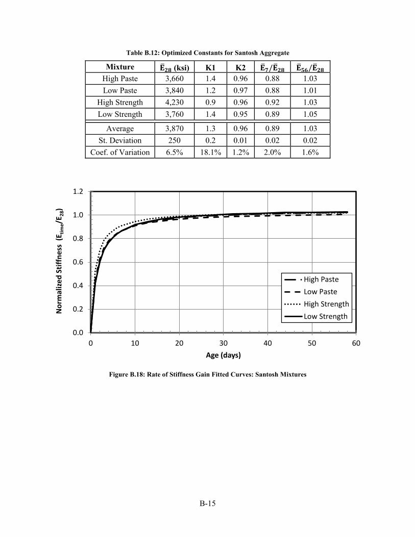
Table B.12: Optimized Constants for Santosh Aggregate
Mixture 𝐄�𝟐𝟖 (ksi) K1 K2 𝐄�𝟕𝟕/𝐄�𝟐𝟖 𝐄�𝟓𝟔𝟔/𝐄�𝟐𝟖 High Paste 3,660 1.4 0.96 0.88 1.03 Low Paste 3,840 1.2 0.97 0.88 1.01
High Strength 4,230 0.9 0.96 0.92 1.03 Low Strength 3,760 1.4 0.95 0.89 1.05
Average 3,870 1.3 0.96 0.89 1.03 St. Deviation 250 0.2 0.01 0.02 0.02
Coef. of Variation 6.5% 18.1% 1.2% 2.0% 1.6%
Figure B.18: Rate of Stiffness Gain Fitted Curves: Santosh Mixtures
0.0
0.2
0.4
0.6
0.8
1.0
1.2
0 10 20 30 40 50 60
Nor
mal
ized
Stiff
ness
(E t
ime/
E 28)
Age (days)
High PasteLow PasteHigh StrengthLow Strength
B-15

B-16

Appendix C: Dry Shrinkage Results
C.1: DRYING SHRINKAGE FITTED CURVES
The fitted drying shrinkage curves from the four laboratory mixtures of each aggregate
source are plotted in the following figures. The fitted drying shrinkage curves from DuPont (3/4-
in.) mixture are excluded in this section, but can be seen in Figure 7.2. The following list of
figures depicts the fitted curves for the four laboratory mixtures of each aggregate source: Figure
C.1 for DuPont (3/8-in.), Figure C.2 for Okanogan Valley, Figure C.3 for Sullivan Road, Figure
C.4 for Pasco, Figure C.5 for Rock Island, and Figure C.6 for Santosh mixtures.
Figure C.1: Fitted Dry Shrinkage Data: DuPont (3/8-in.) Mixtures
0
200
400
600
800
1,000
0 60 120 180 240 300 360
Dryi
ng S
hrin
kage
(mic
rost
rain
)
Drying Duration (days)
High Paste
Low Paste
High Strength
Low Strength
C-1

Figure C.2: Fitted Dry Shrinkage Data: Okanogan Valley Mixtures
Figure C.3: Fitted Dry Shrinkage Sullivan Road Mixtures
0
200
400
600
800
1,000
0 60 120 180 240 300 360
Dryi
ng S
hrin
kage
(mic
rost
rain
)
Drying Duration (days)
High PasteLow PasteHigh StrengthLow Strength
0
200
400
600
800
1,000
0 60 120 180 240 300 360
Dryi
ng S
hrin
kage
(mic
rost
rain
)
Drying Duration (days)
High PasteLow PasteHigh StrengthLow Strength
C-2

Figure C.4: Fitted Dry Shrinkage Data: Pasco Mixtures
Figure C.5: Fitted Dry Shrinkage Data: Rock Island Mixtures
0
200
400
600
800
1,000
0 60 120 180 240 300 360
Dryi
ng S
hrin
kage
(mic
rost
rain
)
Drying Duration (days)
High PasteLow PasteHigh StrengthLow Strength
0
200
400
600
800
1,000
0 60 120 180 240 300 360
Dryi
ng S
hrin
kage
(mic
rost
rain
)
Drying Duration (days)
High PasteLow PasteHigh StrengthLow Strength
C-3

Figure C.6: Fitted Dry Shrinkage Data: Santosh Mixtures
C.2: DRYING SHRINKAGE FITTED CURVE VS. AASHTO PREDICTED CURVE
The fitted curves from the drying shrinkage beams and cylinders of the creep mixtures
are compared against AASHTO specifications (5.4.2.3.3, Equation 2.9) in the following figures.
The fitted curves from the drying shrinkage beams and cylinders of the DuPont (3/4-in.) high-
paste mixture are excluded in this section, but can be seen in Figure 7.4. The following list of
figures depicts the fitted curves for the drying shrinkage beams and cylinders for creep mixtures:
Figure C.7 for DuPont (3/4-in.) low-paste, Figure C.8 for DuPont (3/8-in.) high-paste, Figure C.9
for DuPont (3/8-in.) low-paste, Figure C.10 for Sullivan Road high-paste, and Figure C.11 for
Sullivan Road low-paste mixture.
0
200
400
600
800
1,000
0 60 120 180 240 300 360
Dryi
ng S
hrin
kage
(mic
rost
rain
)
Drying Duration (days)
High PasteLow PasteHigh StrengthLow Strength
C-4
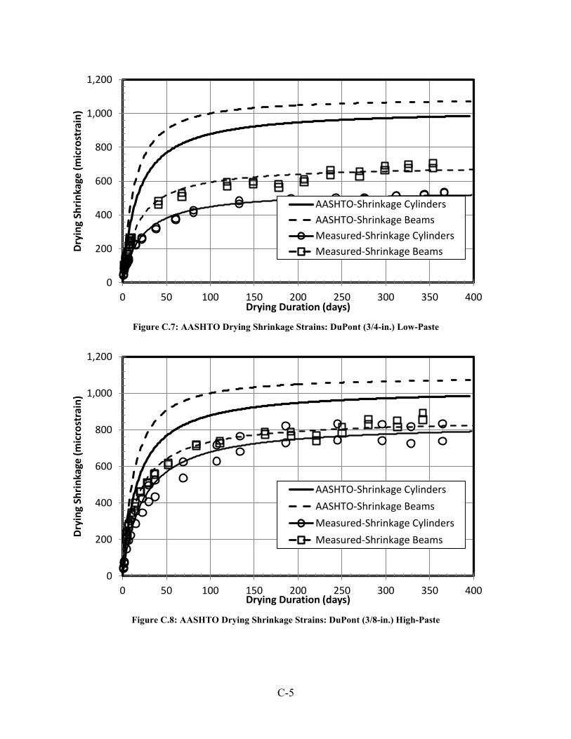
Figure C.7: AASHTO Drying Shrinkage Strains: DuPont (3/4-in.) Low-Paste
Figure C.8: AASHTO Drying Shrinkage Strains: DuPont (3/8-in.) High-Paste
0
200
400
600
800
1,000
1,200
0 50 100 150 200 250 300 350 400
Dryi
ng S
hrin
kage
(mic
rost
rain
)
Drying Duration (days)
AASHTO-Shrinkage CylindersAASHTO-Shrinkage BeamsMeasured-Shrinkage CylindersMeasured-Shrinkage Beams
0
200
400
600
800
1,000
1,200
0 50 100 150 200 250 300 350 400
Dryi
ng S
hrin
kage
(mic
rost
rain
)
Drying Duration (days)
AASHTO-Shrinkage CylindersAASHTO-Shrinkage BeamsMeasured-Shrinkage CylindersMeasured-Shrinkage Beams
C-5

Figure C.9: AASHTO Drying Shrinkage Strains: DuPont (3/8-in.) Low-Paste
Figure C.10: AASHTO Drying Shrinkage Strains: Sullivan Road High-Paste
0
200
400
600
800
1,000
1,200
0 50 100 150 200 250 300 350 400
Dryi
ng S
hrin
kage
(mic
rost
rain
)
Drying Duration (days)
AASHTO-Shrinkage CylindersAASHTO-Shrinkage BeamsMeasured-Shrinkage CylindersMeasured-Shrinkage Beams
0
200
400
600
800
1,000
1,200
0 50 100 150 200 250 300 350 400
Dryi
ng S
hrin
kage
(mic
rost
rain
)
Drying Duration (days)
AASHTO-Shrinkage CylindersAASHTO-Shrinkage BeamsMeasured-Shrinkage CylindersMeasured-Shrinkage Beams
C-6
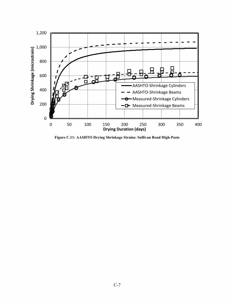
Figure C.11: AASHTO Drying Shrinkage Strains: Sullivan Road High-Paste
0
200
400
600
800
1,000
1,200
0 50 100 150 200 250 300 350 400
Dryi
ng S
hrin
kage
(mic
rost
rain
)
Drying Duration (days)
AASHTO-Shrinkage CylindersAASHTO-Shrinkage BeamsMeasured-Shrinkage CylindersMeasured-Shrinkage Beams
C-7

C-8
Appendix D: Creep Results
D.1: INITIAL GAUGE LENGTHS
The sealed and unsealed creep samples (two of each sample) were placed into the rig
after fourteen days of curing. The gauge lengths of each creep sample were then measured, as per
ASTM C512, to determine the starting lengths of each set of gauges. The creep samples were
then loaded to the targeted thirty-five percent of the Day 14 compressive strength with a
hydraulic ram. Once the required load was applied to the creep rig, locking nuts were fastened to
maintain the stress on the samples. The lengths of each set of gauges were then measured again
to record the deformation due to the application of the axial load on the samples.
The process of applying the load, fastening the nuts, and then measuring each set of
gauges took around five minutes. This time allowed early creep deformations to take place
between the first loading and initial readings. In order to remove that early creep from the
measured data, the initial gauge lengths were extrapolated from the monitored values to a time of
zero. This initial length also removes the elastic deformations, so only the time-dependent
deformations are measured. To show an example of this process, the extrapolated initial length is
shown from DuPont (3/4-in.) high-paste mixture (Unsealed Cylinder #1, north gauge set) in
Figure D.1.
D-1

Figure D.1: Extrapolated Initial Lengths: DuPont (3/4-in.) High-Paste Mixture
D.2: TIME-DEPENDENT DEFORMATIONS
The monitored time-dependent strains and fitted curves from the creep (sealed and
unsealed) and drying shrinkage cylinders are shown in this section for each aggregate source.
The time-dependent strains from DuPont (3/4-in.) high-paste mixture are excluded in this
section, but can be seen in Figure 8.1. The following list of figures depicts the monitored time-
depended strains and fitted curves for each cylinder type and aggregate source: Figure D.2 for
DuPont (3/4-in.) low-paste, Figure D.3 for DuPont (3/8-in.) high-paste, Figure D.4 for DuPont
(3/8-in.) low-paste, Figure D.5 for Sullivan Road high-paste, and Figure D.6 for Sullivan Road
low-paste mixture.
9.985
9.990
9.995
10.000
0.0 0.4 0.8 1.2
Gau
ge L
engt
h (in
)
Time (LN (Days))
Starting Length (Unloaded)Monitored Lengths (Loaded)Extrapolated Initial Length
Elastic Deformation
D-2

Figure D.2: Long-Term Deformations: DuPont (3/4-in.) Low-Paste
Figure D.3: Long-Term Deformations: DuPont (3/8-in.) High-Paste
0
200
400
600
800
1,000
1,200
1,400
1,600
1,800
0 50 100 150 200 250 300 350 400
Stra
in (m
icro
stra
in)
Creep Duration (days)
Unsealed CreepSealed CreepDrying Shrinkage
0
200
400
600
800
1,000
1,200
1,400
1,600
1,800
0 50 100 150 200 250 300 350 400
Stra
in (m
icro
stra
in)
Creep Duration (days)
Unsealed CreepSealed CreepDrying Shrinkage
D-3
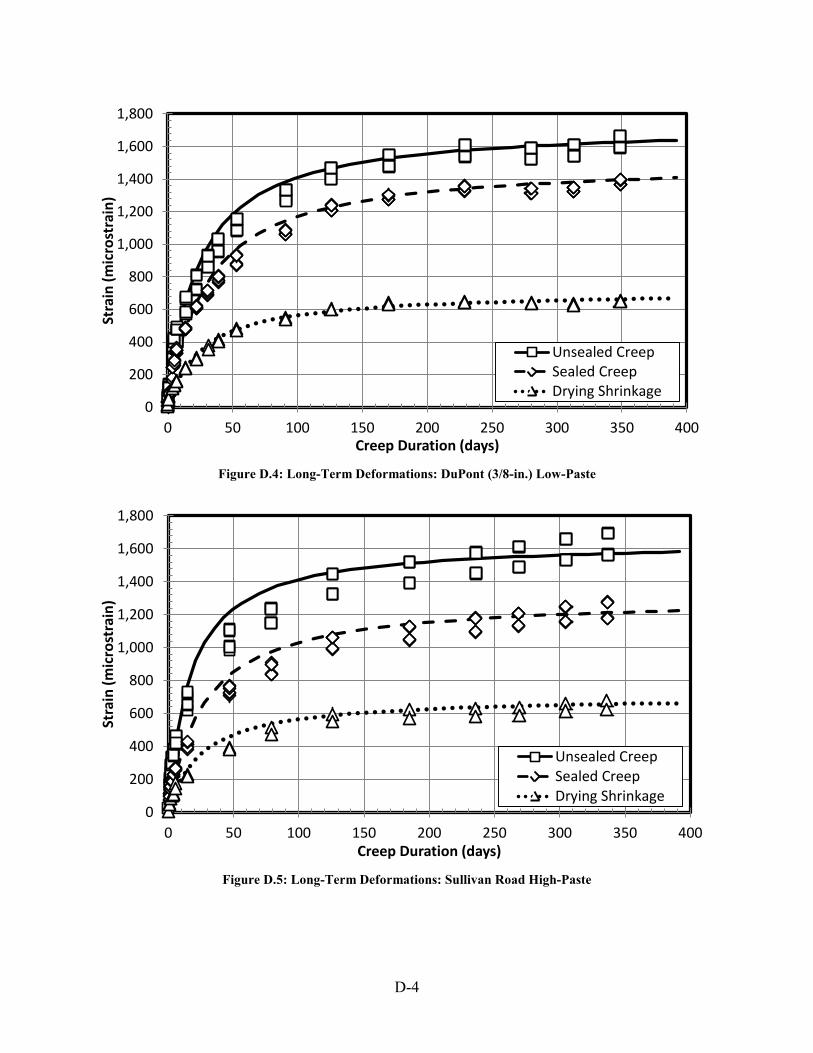
Figure D.4: Long-Term Deformations: DuPont (3/8-in.) Low-Paste
Figure D.5: Long-Term Deformations: Sullivan Road High-Paste
0
200
400
600
800
1,000
1,200
1,400
1,600
1,800
0 50 100 150 200 250 300 350 400
Stra
in (m
icro
stra
in)
Creep Duration (days)
Unsealed CreepSealed CreepDrying Shrinkage
0
200
400
600
800
1,000
1,200
1,400
1,600
1,800
0 50 100 150 200 250 300 350 400
Stra
in (m
icro
stra
in)
Creep Duration (days)
Unsealed CreepSealed CreepDrying Shrinkage
D-4
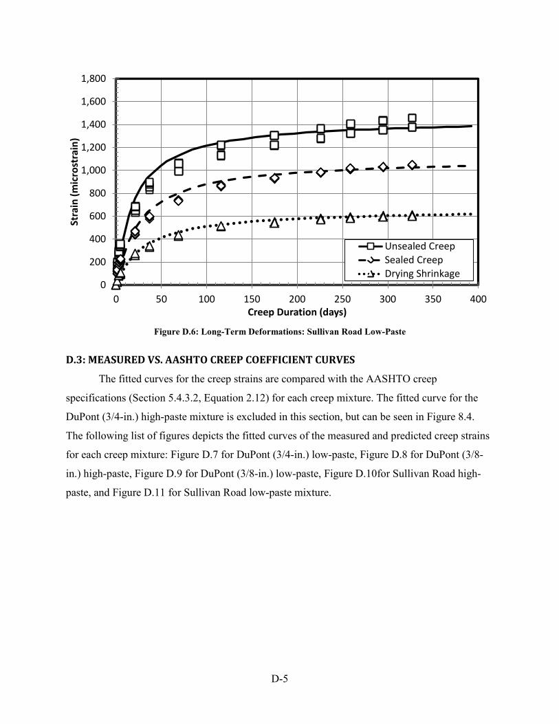
Figure D.6: Long-Term Deformations: Sullivan Road Low-Paste
D.3: MEASURED VS. AASHTO CREEP COEFFICIENT CURVES
The fitted curves for the creep strains are compared with the AASHTO creep
specifications (Section 5.4.3.2, Equation 2.12) for each creep mixture. The fitted curve for the
DuPont (3/4-in.) high-paste mixture is excluded in this section, but can be seen in Figure 8.4.
The following list of figures depicts the fitted curves of the measured and predicted creep strains
for each creep mixture: Figure D.7 for DuPont (3/4-in.) low-paste, Figure D.8 for DuPont (3/8-
in.) high-paste, Figure D.9 for DuPont (3/8-in.) low-paste, Figure D.10for Sullivan Road high-
paste, and Figure D.11 for Sullivan Road low-paste mixture.
0
200
400
600
800
1,000
1,200
1,400
1,600
1,800
0 50 100 150 200 250 300 350 400
Stra
in (m
icro
stra
in)
Creep Duration (days)
Unsealed CreepSealed CreepDrying Shrinkage
D-5

Figure D.7: AASHTO Predicted Creep Coefficient: DuPont (3/4-in.) Low-Paste
Figure D.8: AASHTO Predicted Creep Coefficient: DuPont (3/8-in.) High-Paste
0.0
0.4
0.8
1.2
1.6
2.0
2.4
0 50 100 150 200 250 300 350 400
Cree
p Co
effic
ient
(mic
rost
rain
/ ks
i)
Creep Duration (days)
DuPont (3/4") - LP, CreepAASHTO, Creep Coefficient
0.0
0.4
0.8
1.2
1.6
2.0
2.4
0 50 100 150 200 250 300 350 400
Cree
p Co
effic
ient
(mic
rost
rain
/ ks
i)
Creep Duration (days)
DuPont (3/8") - HP, CreepAASHTO, Creep Coefficient
D-6

Figure D.9: AASHTO Predicted Creep Coefficient: DuPont (3/8-in.) Low-Paste
Figure D.10: AASHTO Predicted Creep Coefficient: Sullivan Road High-Paste
0.0
0.4
0.8
1.2
1.6
2.0
2.4
0 50 100 150 200 250 300 350 400
Cree
p Co
effic
ient
(mic
rost
rain
/ ks
i)
Creep Duration (days)
DuPont (3/8") - LP, CreepAASHTO, Creep Coefficient
0.0
0.4
0.8
1.2
1.6
2.0
2.4
0 50 100 150 200 250 300 350 400
Cree
p Co
effic
ient
(mic
rost
rain
/ ks
i)
Creep Duration (days)
Spokane - HP, CreepAASHTO, Creep Coefficient
D-7

Figure D.11: AASHTO Predicted Creep Coefficient: Sullivan Road Low-Paste
D.4: MEASURED VS. AASHTO CREEP STRAIN EVALUATION
Creep coefficient is calculated by dividing the creep strain with the elastic strain from the
initial loading on the concrete. The AASHTO creep coefficient specifications (5.4.3.2, Equation
2.12) can be used to estimate the creep strain at any loading duration. The accuracy of creep
strain prediction from AASHTO depends greatly on the calculated elastic deformation. To
illustrate this dependence, the creep strains were determined from elastic strain values based on
three sets of assumptions:
• The first elastic strain was calculated using the AASHTO predicted elastic modulus
(5.4.2.4-1, Equation 2.7) based on the design strength of the mixture (4,000 psi) along
with the applied stress (Table 8.7).
• The second elastic strain was calculated using the predicted elastic modulus value
(5.4.2.4-1, Equation 2.7) from the measured Day 14 compressive strength (Table 8.8)
along with the applied stress (Table 8.7).
• The third elastic strain value was the measured strain value from the initial loading (Table
8.8).
0.0
0.4
0.8
1.2
1.6
2.0
2.4
0 50 100 150 200 250 300 350 400
Cree
p Co
effic
ient
(mic
rost
rain
/ ks
i)
Creep Duration (days)
Spokane - LP, CreepAASHTO, Creep Coefficient
D-8
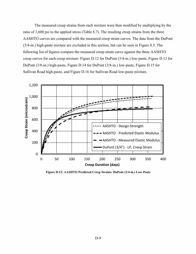
The measured creep strains from each mixture were then modified by multiplying by the
ratio of 1,600 psi to the applied stress (Table 8.7). The resulting creep strains from the three
AASHTO curves are compared with the measured creep strain curves. The data from the DuPont
(3/4-in.) high-paste mixture are excluded in this section, but can be seen in Figure 8.5. The
following list of figures compare the measured creep strain curve against the three AASHTO
creep curves for each creep mixture: Figure D.12 for DuPont (3/4-in.) low-paste, Figure D.13 for
DuPont (3/8-in.) high-paste, Figure D.14 for DuPont (3/8-in.) low-paste, Figure D.15 for
Sullivan Road high-paste, and Figure D.16 for Sullivan Road low-paste mixture.
Figure D.12: AASHTO Predicted Creep Strains: DuPont (3/4-in.) Low-Paste
0
200
400
600
800
1,000
1,200
0 50 100 150 200 250 300 350 400
Cree
p St
rain
(mic
rost
rain
)
Creep Duration (days)
AASHTO - Design Strength
AASHTO - Predicted Elastic Modulus
AASHTO - Measured Elastic Modulus
DuPont (3/4") - LP, Creep Strain
D-9
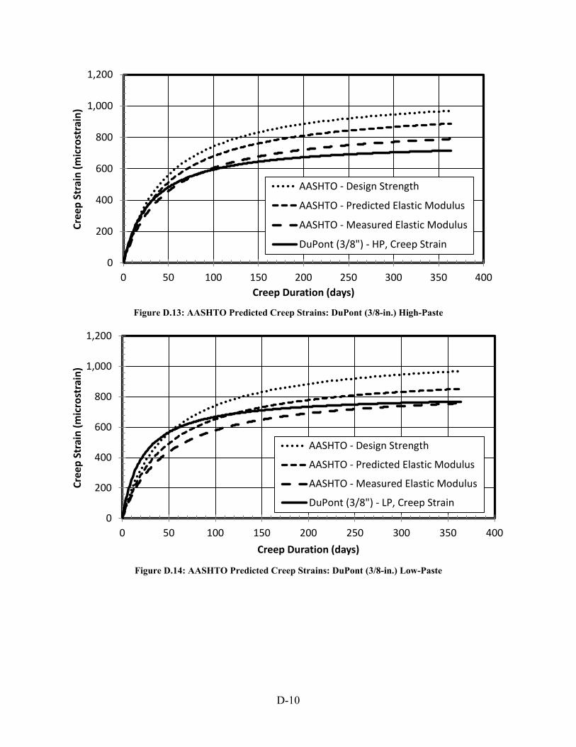
Figure D.13: AASHTO Predicted Creep Strains: DuPont (3/8-in.) High-Paste
Figure D.14: AASHTO Predicted Creep Strains: DuPont (3/8-in.) Low-Paste
0
200
400
600
800
1,000
1,200
0 50 100 150 200 250 300 350 400
Cree
p St
rain
(mic
rost
rain
)
Creep Duration (days)
AASHTO - Design Strength
AASHTO - Predicted Elastic Modulus
AASHTO - Measured Elastic Modulus
DuPont (3/8") - HP, Creep Strain
0
200
400
600
800
1,000
1,200
0 50 100 150 200 250 300 350 400
Cree
p St
rain
(mic
rost
rain
)
Creep Duration (days)
AASHTO - Design Strength
AASHTO - Predicted Elastic Modulus
AASHTO - Measured Elastic Modulus
DuPont (3/8") - LP, Creep Strain
D-10
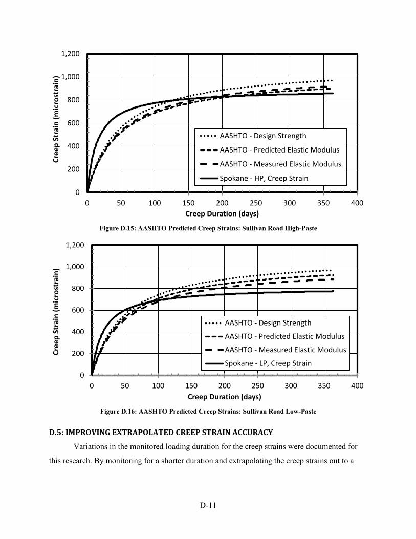
Figure D.15: AASHTO Predicted Creep Strains: Sullivan Road High-Paste
Figure D.16: AASHTO Predicted Creep Strains: Sullivan Road Low-Paste
D.5: IMPROVING EXTRAPOLATED CREEP STRAIN ACCURACY
Variations in the monitored loading duration for the creep strains were documented for
this research. By monitoring for a shorter duration and extrapolating the creep strains out to a
0
200
400
600
800
1,000
1,200
0 50 100 150 200 250 300 350 400
Cree
p St
rain
(mic
rost
rain
)
Creep Duration (days)
AASHTO - Design Strength
AASHTO - Predicted Elastic Modulus
AASHTO - Measured Elastic Modulus
Spokane - HP, Creep Strain
0
200
400
600
800
1,000
1,200
0 50 100 150 200 250 300 350 400
Cree
p St
rain
(mic
rost
rain
)
Creep Duration (days)
AASHTO - Design Strength
AASHTO - Predicted Elastic Modulus
AASHTO - Measured Elastic Modulus
Spokane - LP, Creep Strain
D-11

year, strain values can be predicted with a lower required testing duration. As Section 8.3
describes, longer testing durations improved the accuracy of the extrapolated creep strain values.
To offset this inaccuracy of shorter monitoring durations, a coefficient was determined based on
the laboratory creep data to multiply the fitted creep curves (optimized from Equation 8.2). For
180 days of creep strain monitoring, a coefficient of 1.1 provided the most consistent
improvement to the extrapolated strain values. For 56 days of monitoring, a coefficient of 1.2
improved the creep data the best.
The improvement of the fitted creep curves from DuPont (3/4-in.) high-paste mixture is
excluded in this section, but can be seen in figures 8.12 and 8.13. The following list of figures
shows the improvement to the modified creep curves from 180 days of monitored data for each
creep mixture: Figure D.17 for DuPont (3/4-in.) low-paste, Figure D.18 for DuPont (3/8-in.)
high-paste, Figure D.19 for DuPont (3/8-in.) low-paste, Figure D.20 for Sullivan Road high-
paste, and Figure D.21 for Sullivan Road low-paste mixture.
Figure D.17: Modified Day 180 Creep Strain Curves: DuPont (3/4-in.) Low-Paste
0
200
400
600
800
1,000
0 50 100 150 200 250 300 350 400
Cree
p St
rain
(mic
rost
rain
)
Creep Duration (days)
365 DaysModified Day 180180 Days
D-12

Figure D.18: Modified Day 180 Creep Strain Curves: DuPont (3/8-in.) High-Paste
Figure D.19: Modified Day 180 Creep Strain Curves: DuPont (3/8-in.) Low-Paste
0
200
400
600
800
1,000
0 50 100 150 200 250 300 350 400
Cree
p St
rain
(mic
rost
rain
)
Creep Duration (days)
365 DaysModified Day 180180 Days
0
200
400
600
800
1,000
0 50 100 150 200 250 300 350 400
Cree
p St
rain
(mic
rost
rain
)
Creep Duration (days)
365 DaysModified Day 180180 Days
D-13
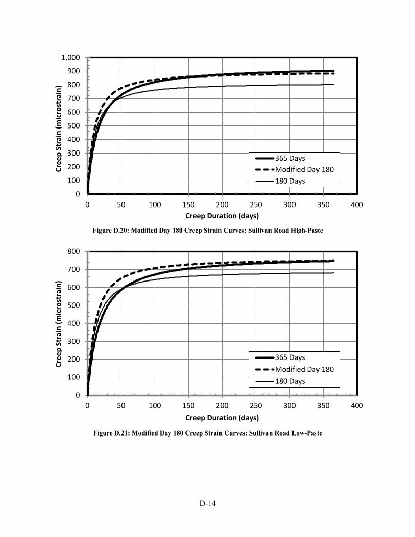
Figure D.20: Modified Day 180 Creep Strain Curves: Sullivan Road High-Paste
Figure D.21: Modified Day 180 Creep Strain Curves: Sullivan Road Low-Paste
0
100
200
300
400
500
600
700
800
900
1,000
0 50 100 150 200 250 300 350 400
Cree
p St
rain
(mic
rost
rain
)
Creep Duration (days)
365 DaysModified Day 180180 Days
0
100
200
300
400
500
600
700
800
0 50 100 150 200 250 300 350 400
Cree
p St
rain
(mic
rost
rain
)
Creep Duration (days)
365 DaysModified Day 180180 Days
D-14

The following list of figures shows the improvement to the modified creep curves from
56 days of monitored data for each creep mixture: Figure D.22 for DuPont (3/4-in.) low-paste,
Figure D.23 for DuPont (3/8-in.) high-paste, Figure D.24 for DuPont (3/8-in.) low-paste, Figure
D.25 for Sullivan Road high-paste, and Figure D.26 for Sullivan Road low-paste mixture.
Figure D.22: Modified Day 56 Creep Strain Curves: DuPont (3/4-in.) Low-Paste
0
200
400
600
800
1,000
0 50 100 150 200 250 300 350 400
Cree
p St
rain
(mic
rost
rain
)
Creep Duration (days)
365 DaysModified Day 5656 Days
D-15
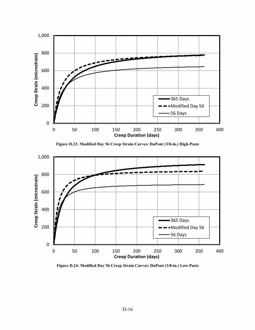
Figure D.23: Modified Day 56 Creep Strain Curves: DuPont (3/8-in.) High-Paste
Figure D.24: Modified Day 56 Creep Strain Curves: DuPont (3/8-in.) Low-Paste
0
200
400
600
800
1,000
0 50 100 150 200 250 300 350 400
Cree
p St
rain
(mic
rost
rain
)
Creep Duration (days)
365 DaysModified Day 5656 Days
0
200
400
600
800
1,000
0 50 100 150 200 250 300 350 400
Cree
p St
rain
(mic
rost
rain
)
Creep Duration (days)
365 DaysModified Day 5656 Days
D-16

Figure D.25: Modified Day 56 Creep Strain Curves: Sullivan Road High-Paste
Figure D.26: Modified Day 56 Creep Strain Curves: Sullivan Road Low-Paste
0
200
400
600
800
1,000
0 50 100 150 200 250 300 350 400
Cree
p St
rain
(mic
rost
rain
)
Creep Duration (days)
365 DaysModified Day 5656 Days
0
200
400
600
800
1,000
0 50 100 150 200 250 300 350 400
Cree
p St
rain
(mic
rost
rain
)
Creep Duration (days)
365 DaysModified Day 5656 Days
D-17

D-18