structural coupling of high-rise buildings linked …
TRANSCRIPT

STRUCTURAL COUPLING OF HIGH-RISE BUILDINGS LINKED BY
SKYBRIDGES
A Thesis
by
ATHEER KHUDHUR JUMAAH
Submitted to the Office of Graduate and Professional Studies of
Texas A&M University
in partial fulfillment of the requirements for the degree of
MASTER OF SCIENCE
Chair of Committee, John Niedzwecki
Committee Members, Luciana Barroso
H. Joseph Newton
Head of Department, Robin Autenrieth
August 2017
Major Subject: Civil Engineering
Copyright 2017 Atheer Jumaah

ii
ABSTRACT
An example of the creative building concepts is the connection two or more
buildings using skybridges, which are also referred to as skyways or skywalks. They can
provide direct passage in congested areas, serve to make walking more pleasant for
pedestrian passage and protect walkers from the elements like the scorching heat or heavy
rain. Further in large cities, a skywalk or skybridge can serve to separate the vehicle traffic
from pedestrian traffic.
In this research study, the effect of introducing single skybridge or multiple
skybridges on the dynamic response behavior of the linked high-rise buildings is studied.
A mathematical matrix formulation using 3-D space frames was implemented for time
domain simulations in Matlab and was validated using the finite element software
SAP2000. This included a comparison of translational and rotational mode shapes and
undamped natural frequency estimates, and time series response predictions. The building
systems were excited using very four different strong ground motion time series records.
A grouping of nine specific cases was developed to investigate the response of building
system that connected two buildings of different height. It was found that multiple
skybridge designs influenced the higher modal characteristics and structural response,
suggesting some response optimization was possible. In addition, statistical
characterization of the excitation and response behavior illustrated that non-Gaussian
excitation was filtered by the building system to yielding a reduced non-Gaussian
response.

iii
DEDICATION
To my almighty God, Allah

iv
ACKNOWLEDGEMENTS
All of the praise is due to Allah; I ask him for his direction and forgiveness. I would
really wish to extend my appreciation to my parents, father, and mother before she passed
away, who constantly endeavor to make me a prosperous person, and I seek to please
them. I would like to give thanks to my family members, Liqaa, Ahmad, Alaa, Diana,
Sarah, and my niece Alaa for their motivation and being supportive. My appreciations to
my committee chair Professor John Niedzwecki for his useful directions. I have had an
outstanding experience with him during my research course. I would as well say thanks to
my committee members Professor Luciana Barroso and Professor H. Joseph Newton for
assisting me. My thanks to Layal Almaddah, my officemates, and all friends for being
positive in my life. I am really thankful to the Higher Committee for Education
Development in Iraq (HCED) for their financial assistance. I thank Texas A&M
University for being an extraordinary university for students from various places
worldwide. My distinctive thanks to the Zachry Department of Civil Engineering- Faculty,
staff, and students-.

v
CONTRIBUTORS AND FUNDING SOURCES
This work was supervised by a thesis committee consisting of Professor John
Niedzwecki [advisor] and Professor Luciana Barroso of Zachry Department of Civil
Engineering and Professor H. Joseph Newton of Department of Statistics.
All work for the thesis was completed independently by the student.
Graduate study was supported by a scholarship from the Higher Committee for
Educational Development in Iraq (HCED).

vi
TABLE OF CONTENTS
Page
ABSTRACT .............................................................................................................. ii
DEDICATION .......................................................................................................... iii
ACKNOWLEDGEMENTS ...................................................................................... iv
CONTRIBUTORS AND FUNDING SOURCES ..................................................... v
TABLE OF CONTENTS .......................................................................................... vi
LIST OF FIGURES ................................................................................................... viii
LIST OF TABLES .................................................................................................... xii
1. INTRODUCTION ............................................................................................... 1
1.1 Background and Problem Statement .................................................... 1
1.2 Research Objective and Plan ................................................................ 6
2. BUILDING AND SKYBRIDGE MODEL DEVELOPMENT .......................... 10
2.1 Engineering Models with Different Levels of Complexity .................. 10
2.2 General Matrix Formulation ................................................................ 16
2.2.1 Inertial Force ............................................................................... 16
2.2.2 Elastic Force ............................................................................... 18
2.2.3 Skybridge Considerations .......................................................... 23
2.2.4 Transformation of coordinates ................................................... 24
2.2.5 Damping Force ........................................................................... 30
3. MATLAB CODE VALIDATION ...................................................................... 31
3.1 Verification Model Number One (VM1) ............................................. 32
3.2 Verification Model Number Two (VM21) ........................................... 36
3.3 Verification Model Number Three (VM3) ........................................... 39

vii
Page
4. ISOLATED AND COUPLED HIGH-RISE BUILDING SIMULATIONS ............. 48
4.1 Undamped Twin High-rise Building System ...................................... 48
4.2 Undamped Different High-Rise Building System ............................... 55
4.3 Damped Different High-Rise Building System ................................... 59
5. SKYBRIDGE SIMULATIONS ................................................................................ 62
5.1 Skybridge Connection End Conditions ................................................ 62
5.2 Skybridge Stiffness .............................................................................. 66
5.3 Location of a Skybridge ....................................................................... 69
5.4 Number of Skybridges ......................................................................... 71
5.3 Statistical Characterization of the Excitation and Response ................ 74
6. SUMMARY AND CONCLUSIONS ........................................................................ 82
REFERENCES .......................................................................................................... 87
APPENDIX A ........................................................................................................... 90
APPENDIX B ........................................................................................................... 95

viii
LIST OF FIGURES
Page
Figure 1. Petronas Twin Tower Skybridge (Printed from Rogers, 2017) .......................... 3
Figure 2. Bahrain World Trade Center (Printed from Lomholt, Lomholt, Solkoff, &
Solkoff, 2017) .................................................................................................... 3
Figure 3. Overview of the research plan ............................................................................ 8
Figure 4. Twin buildings linked by a skybridge ................................................................. 9
Figure 5. Different buildings linked by a skybridge .......................................................... 9
Figure 6. Different buildings linked by three skybridges ................................................... 9
Figure 7. Two independent high-rise buildings ............................................................... 10
Figure 8. Dynamic degrees of freedom for two independent buildings ........................... 11
Figure 9. Circular Skybridge (Printed from "The World's Best Photos of skybridge
and way - Flickr Hive Mind", 2017) ................................................................ 12
Figure 10. Rectangular Skybridge (Printed from "Skyway or the highway for
teaching hospital - Austin Monitor", 2017) .................................................... 12
Figure 11. Truss skybridge with roller connections ......................................................... 13
Figure 12. Frame skybridge with fixed connections ........................................................ 13
Figure 13. Two linked high-rise buildings ....................................................................... 14
Figure 14. Dynamic degrees of freedom for two linked buildings .................................. 15
Figure 15. Two linked lumped masses ............................................................................. 17
Figure 16. Free body diagram of a frame member in a 3D-space along x-axis ............... 19
Figure 17. Shape coupling in coupled buildings .............................................................. 23

ix
Page
Figure 18. Free body diagram of a frame member in a 3D-space with an angle of
rotation (α) ...................................................................................................... 25
Figure 19. Free body diagram of a frame member in a 3D-space with an angle of
rotation (β) ...................................................................................................... 27
Figure 20. Verification model one (VM1) ....................................................................... 32
Figure 21. Dynamic response of VM1 by Matlab (u and w are identical) ....................... 35
Figure 22. Dynamic response of VM1by SAP2000 (u and w are identical) .................... 35
Figure 23. Verification model two (VM2) ....................................................................... 36
Figure 24. Verification model three (VM3) ..................................................................... 40
Figure 25. Horizontal displacement (u) at m10 and m14 of VM3 by Matlab .................... 42
Figure 26. Horizontal displacement (u) at m10 and m14 of VM3 by SAP2000 ................ 43
Figure 27. Horizontal displacement (w) at m10 and m14 of VM3 by Matlab .................... 43
Figure 28. Horizontal displacement (w) at m10 and m14 of VM3 by SAP2000 ............... 44
Figure 29. Torsional displacement (y) at m10 and m14 of VM3 by Matlab ...................... 44
Figure 30. Torsional displacement (y) at m10 and m14 of VM3 by SAP2000 .................. 45
Figure 31. First two modes in x-direction for VM3 by Matlab ........................................ 46
Figure 32. First two modes in coupled y-direction for VM3 by Matlab .......................... 46
Figure 33. Horizontal displacement (u) at m15 (H=210 feet) in HBS1 using Multiple
masses .............................................................................................................. 50
Figure 34. Horizontal displacement (u) at m15 (H=210 feet) in HBS1 using a single
mass concentrated at 8th floor ......................................................................... 51
Figure 35. Horizontal displacement (u) at m15 (H=210 feet) in HBS1 using a single
mass concentrated at 6th floor ........................................................................ 52

x
Page
Figure 36. Horizontal displacement (u) at m15 (H=210 feet) in HBS1 using a single
mass concentrated at 10th floor ...................................................................... 52
Figure 37. Horizontal displacement (u) at m15 (H=210 feet) in HBS1 using a single
mass concentrated at 12th floor ...................................................................... 53
Figure 38. Horizontal displacement (u) at m15 (H=210 feet) in HBS1 using a single
mass concentrated at 15th floor ....................................................................... 53
Figure 39. Horizontal displacement (u) of uncoupled HBS2 at m15 (H=210 feet) .......... 57
Figure 40. Horizontal displacement (w) of uncoupled HBS2 at m15 (H=210 feet) .......... 57
Figure 41. Horizontal displacement (u) of coupled HBS2 at m15 (H=210 feet) ............... 58
Figure 42. Horizontal displacement (w) of coupled HBS2 at m15 (H=210 feet) .............. 58
Figure 43. Horizontal displacement (u) of coupled HBS2 at m15 (H=210 feet),
(x=0.02) .......................................................................................................... 59
Figure 44. Horizontal displacement (w) of coupled HBS2 at m15 (H=210 feet),
(x=0.02) .......................................................................................................... 60
Figure 45. Change of horizontal displacement (wmax) at m20 (H=280 feet) with the
damping ratio .................................................................................................. 60
Figure 46. Change of the number of cycles for horizontal displacement (w) at m20
(H=280 feet) to drop to (10%) of the maximum value relative to the
damping ratio .................................................................................................. 61
Figure 47. Horizontal displacements in x-direction (u) and z-direction (w) of HBS3
with a roller ends skybridge ........................................................................... 64
Figure 48. Horizontal displacements in x-direction (u) and z-direction (w) of HBS3
with a hinge ends skybridge ........................................................................... 65
Figure 49. Dynamic displacements (u) and (w) of HSB3 with a fixed ends skybridge ... 66
Figure 50. Change of horizontal displacement (u) of mt (H=308 feet) and ms
(H=154 feet) at the twenty-second floor with change of the normalized
axial rigidity .................................................................................................. 68

xi
Page
Figure 51. Change of horizontal displacement (w) of mt (H=308 feet) and ms
(H=154 feet) with change of the normalized flexural rigidity ....................... 68
Figure 52. Change of horizontal displacement (u) of mt (H=308 feet) and ms
(H=154 feet) with the location of the skybridge ............................................ 70
Figure 53. Change of horizontal displacement (w) of mt (H=308 feet) and ms
(H=154 feet) with the location of the skybridge ............................................ 70
Figure 54. Change of horizontal displacement (u) of mt (H=308 feet) and ms
(H=154 feet) with number of skybridges (N) ................................................. 72
Figure 55. Change of horizontal displacement (w) of mt (H=308 feet) and ms
(H=154 feet) with number of skybridges (N) ................................................. 73
Figure 56. Change of natural frequencies of x-direction with N...................................... 74
Figure 57. Normal distribution of (u) with a skybridge (El-Centro) ................................ 80
Figure 58. Normal distribution of (u) with three skybridges (El-Centro) ........................ 80
Figure 59. Normal distribution of (w) with a skybridge (Northridge) ............................. 81
Figure 60. Normal distribution of (w) with three skybridges (Northridge) ..................... 81
Figure 61. The 1940 El-Centro earthquake record ........................................................... 95
Figure 62. The 1940 El-Centro power spectral density.................................................... 96
Figure 63. The 1994 Northridge earthquake record ......................................................... 96
Figure 64. The 1994 Northridge power spectral density .................................................. 97
Figure 65. The Umbro-Marchigiano earthquake record .................................................. 97
Figure 66. The Umbro-Marchigiano power spectral density ........................................... 98
Figure 67. The artificial NF-17 earthquake record........................................................... 98
Figure 68. The artificial NF-17 power spectral density ................................................... 99

xii
LIST OF TABLES
Page
Table 1. Verification models ............................................................................................ 31
Table 2. Natural frequencies for verification model one (VM1) ..................................... 33
Table 3. Mode shapes for verification model one (VM1) ................................................ 34
Table 4. Mode shapes for verification model two (MV2) ................................................ 37
Table 5. Natural frequencies for verification model two (VM2) ..................................... 38
Table 6. Natural frequencies for VM3 ............................................................................. 41
Table 7. Structural Properties of B1 and B2 in High-rise building system 1 (HBS1) ..... 48
Table 8. Structural Properties of the Skybridge in HBS1 ................................................ 49
Table 9. Maximum horizontal displacement (u) with respect to different equivalent
mass locations ................................................................................................... 54
Table 10. Different dynamic characteristics of the skybridge in HBS1 ........................... 55
Table 11. Structural properties of B1 in HBS2 ................................................................ 56
Table 12. Structural properties of B2 in HBS2 ................................................................ 56
Table 13. Structural properties of B1 in HSB3 ................................................................ 63
Table 14. Structural properties of B2 in HSB3 ................................................................ 63
Table 15. Geometrical properties of B1 in HSB4 ............................................................ 66
Table 16. Geometrical properties of B2 in HSB4 ............................................................ 67
Table 17. Number of skybridges and their locations ....................................................... 71
Table 18. Statistical analysis of earthquake records ........................................................ 75

xiii
Page
Table 19. The dominant frequencies of earthquake records ............................................ 75
Table 20. Geometrical Properties of B1 in HBS5 ............................................................ 76
Table 21. Geometrical properties of B2 in HBS5 ............................................................ 76
Table 22. Geometrical properties of the skybridge in HBS5 ........................................... 76
Table 23. Statistical characterization of HBS5 response subjected to the 1940
El-Centro record .............................................................................................. 78
Table 24. Statistical characterization of HBS5 response subjected to the 1994
Northridge record ............................................................................................. 79
Table 25. Case studies that were considered in this research study ................................. 84

1
1. INTRODUCTION
1.1. Background and Problem Statement
As Architectural firms develop creative building concepts to meet the demands
of their clients, the structural design often becomes quite complicated. An example of the
architectural complexity is the connection two or more buildings using skybridges, also
referred to as skyways or skywalks. This concept can also be used to provide connections
at several elevations on buildings. Generally, a skybridge is intended to serve as a
walkway to facilitate pedestrian traffic between buildings and, depending on the skybridge
location and elevation, they can provide a spectacular view for pedestrians walking
between the connected structures. One example is the distinctive Petronas Twin Towers
in Malaysia that are connected by a single skywalk is shown in figure 1. Another example
is the Bahrain World Trade Center buildings shown in figure 2. This example is quite
interesting as it was designed with multiple skyways that each incorporate a wind turbine.
There are many other architectural concepts for the use of skybridges that include gardens
and swimming pools.
The use of skybridges to connect buildings can significantly influence the dynamic
structural response behavior when these high-rise buildings are subjected to loads
involving extreme winds and/or strong ground motions. In comparison, the impact of
these loads is expected to be less severe for low-rise buildings. Most of the previous
studies have focused the modeling of two identical buildings connected by a single
skybridge and subject to various wind loading scenarios. This research study will focus

2
on the bending and torsional response of high-rise buildings subject to strong ground
motions where the buildings need not be identical and multiple skybridge connections are
possible.
Lim, Bienkiewicz, & Richards (2011) conducted research in order to study the
influence of a single skybridge on the dynamic response behavior of two interconnected
identical high-rise buildings. They modeled two high-rise buildings interconnected by a
skybridge at the mid-height of each building. In their study, each building was idealized
as a MDOF lumped mass model interconnected by a frame element representing the
skybridge. They were able to realize that x-in and x-out mode shapes, related to the motion
along the axis that is perpendicular to skybridge, are not coupled to other mode shapes.
Other modes in the z-direction and torsional modes are coupled. In addition, approximate
empirical formulas were introduced to calculate natural frequencies for all mode shapes.
The structural system was modeled using a six-degree of freedom representation where
the buildings were specified to have identical dynamic properties.

3
Figure 1. Petronas Twin Tower Skybridge (Printed from Rogers, 2017) Figure 2. Bahrain World Trade Center (Printed from Lomholt,
Lomholt, Solkoff, & Solkoff, 2017)
4
Effects of structural and aerodynamic couplings on the dynamic response of high-
rise twin buildings with a skybridge was also studied by Lim & Bienkiewicz (2009) using
a high-frequency force balance (HFFB) technique. In these research studies, they utilized
the same structural system model described in the previous research study (Lim,
Bienkiewicz, & Richards, 2011) and utilized wind tunnel tests to further study the coupled
response behavior. It was realized the inclusion of the structural coupling led to significant
reductions, up to 22% in the resultant rooftop accelerations, when compared with the
maximum accelerations of the structurally uncoupled buildings.
In another study, (Song & Tse, 2014) increased the complexity of the model that
was subjected to wind loads. Each floor in the high-rise building was represented as a
MDOF lumped mass system. The published report does not provide enough data on the
directionally coupled motion. Nonetheless, they reported that having a link connecting
two high-rise buildings might increase the frequencies or reduce them due to the addition
of the mass of the skybridge. Also, they suggested (0.8 H) as the most effective height for
the skybridge that can reduce the dynamic response as much as possible. Another study
(Lee, Kim, & Ko, 2012) considered two different buildings connected by a single
skybridge and subjected to wind and earthquake loads. In addition, evaluation of
coupling–control effect of a skybridge for adjacent high-rise buildings was considered;
they introduced lead rubber bearings (LRB) and linear motion bearings (LMB) to model
the connection between the skybridge and the two buildings. They investigated the
response of the two structures with and without using lead rubbers and linear motion
bearings seeking a means to minimize the dynamic response. They concluded that when

5
the skybridge is rigidly connected to high-rise buildings, the dynamic response increases
because the skybridge increases the irregularity of the building. Another point is that when
using LRBs, the dissipation increases up to 30 %, and when using dampers additionally to
LRBs, the dissipation increases up to 100%.
In another study, (Zhao, Sun, & Zheng, 2009) discussed the finite-element model
modification of a long steel skybridge to related actual dynamic properties that are
obtained from the full-scale experiment. Analysis results show that the modal assurance
criteria (MAC) values of the correlated structural modal shapes are all close to 1.0, which
indicates a strong correlation between calculated and estimated structural modal shapes.
The coupled building static response analysis of two high-rise buildings was made, and
the modeling of the associated equivalent static wind loads using the HFFB measurement
was presented (Chen & Kareem, 2005). Two building systems, coupled by a link and
uncoupled, were evaluated through both a simple estimation method and spectral analysis,
considering only the axial rigidity of the link (Behnamfar, Dorafshan, Taheri, & Hosseini
Hashemi, 2016). Utilizing a semi-active control system utilizing a cable connecting the
two structures was investigated as to its ability reduce wind-induced oscillation (Klein &
Healey, 1987). A semi-active control system was recommended for a few reasons: an
acceptable cost level, retrofit capability, minimal space requirements, and quite effective
in removing unwanted kinetic energy. From the structural analysis and design perspective,
a research study was conducted to present an optimization of high-rise buildings with
hinge-connected skybridges with respect to those are with roller-connected skybridges
(McCall & Balling, 2016).
6
1.2. Research Objective and Plan
An overview of the research plan is presented in Figure 3. The most common
methods that are used to develop discretized high-rise buildings are finite element models
and shear building models. In this study, the structural designs of existing of skybridges
will be investigated in order to determine how best to model them. Of particular interest,
will be determining the levels of complexity of the models needed in order to better predict
the coupled response behavior of high-rise buildings connected by skybridges. More
specifically, this study will scrutinize the force and moment coupling between skybridges
and high-rise buildings where roller, hinge, or rigid connections are utilized. The selection
of the various end conditions controls the dynamic degrees of freedom and influence the
structural models used in the analysis of the high-rise building system. The structural
model of the linked high-rise buildings will be subjected to a variety of strong ground
motion loading time series records selected from earthquake events such as the 1994
Northridge and the 1940 El-Centro earthquakes in the United States, Umbro-Marchigiano
earthquake in Turkey, Mexico City earthquake in Mexico, and NF17 (a part of SAC
project) in Japan. The data sets will be carefully chosen from these global events to provide
a range of peak ground accelerations and event durations. It is noted that model
simulations in structural dynamics can be pursued in the time domain or frequency
domain. This study will utilize the most effective way to perform the simulations and
present the numerical results.
In this research study, a system of two high-rise buildings will be modeled using
increasing levels of complexity. This will include better representations of the buildings

7
and skywalk geometries and their influence on the dynamic response behavior. Figure 4
presents a basic conservative (undamped) system involving twin high-rise buildings that
are linked by a skybridge. In this case, each building is modeled as a single lumped mass
located at the geometrical center of each building. These lumped masses are then
connected by a frame member representing the skybridge, and based on previous research
studies this has been determined to be a reasonable first pass model. This will be done for
comparative purposes with previous studies. Next, the level of model complexity will be
increased using MDOF models that distribute the mass at each floor of a building, which
is important for cases where the buildings are not identical and connected by multiple
skybridges. The response behavior of these various system models subjected to selected
time domain records of the strong ground motion records will be investigated.
A system of two different high-rise buildings linked by a skybridge is presented in
figure 5, and it represents a more general case that will be investigated. The length of the
time domain simulation noticeably impacts the structurally coupled response of high-rise
buildings linked by a skybridge. Further, the effect of the damping force is expected to
also play a significant role the dynamic behavior, which includes flexure and torsional
motions. A schematic of the multiple skybridge configurations is illustrated in figure 6.
The dynamic response behavior of the building system will be influenced by the mass
distribution, the axial and flexural rigidity of the individual buildings, their elevation, the
skybridge geometrical configurations and the degree of connectivity they provide between
the buildings. The degree to which different configurations will differ will be examined
and quantified. A logical question to be considered is what is an optimal number of

8
skybridges and their elevations that minimize the coupled dynamic response behavior of
the system?
Figure 3. Overview of the research plan

9
Figure 5. Different buildings linked by a
skybridge
Figure 6. Different buildings linked by three skybridges
Figure 4. Twin buildings linked by a skybridge

10
2. BUILDING AND SKYBRIDGE MODEL DEVELOPMENT
2.1. Engineering Models with Different Levels of Complexity
To calculate an approximate dynamic response, a building can be represented by
an equivalent single lumped mass. Hence, a system of two independent buildings is
modeled using two independent lumped masses. The geometry of the two independent
buildings with respect to the global axis is indicated in figure 7.
Figure 7. Two independent high-rise buildings
11
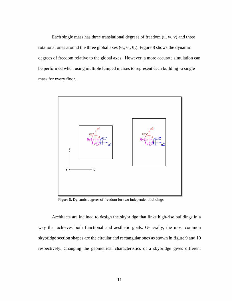
Each single mass has three translational degrees of freedom (u, w, v) and three
rotational ones around the three global axes (θx, θz, θy). Figure 8 shows the dynamic
degrees of freedom relative to the global axes. However, a more accurate simulation can
be performed when using multiple lumped masses to represent each building -a single
mass for every floor.
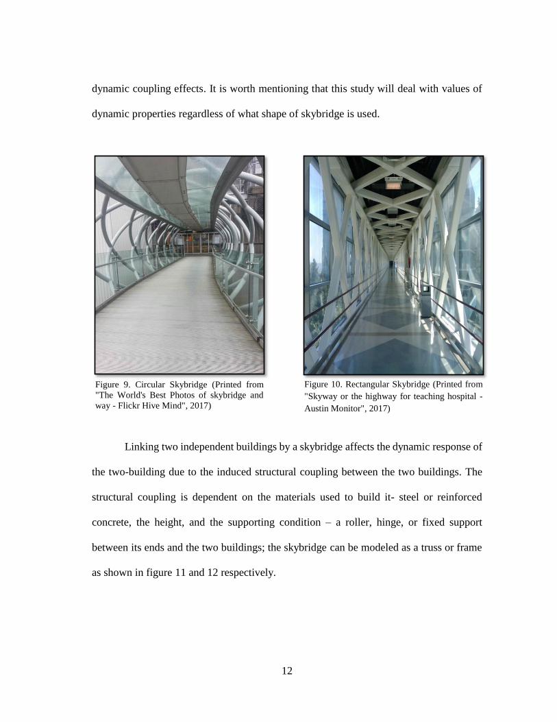
Architects are inclined to design the skybridge that links high-rise buildings in a
way that achieves both functional and aesthetic goals. Generally, the most common
skybridge section shapes are the circular and rectangular ones as shown in figure 9 and 10
respectively. Changing the geometrical characteristics of a skybridge gives different
Figure 8. Dynamic degrees of freedom for two independent buildings
12
dynamic coupling effects. It is worth mentioning that this study will deal with values of
dynamic properties regardless of what shape of skybridge is used.
Linking two independent buildings by a skybridge affects the dynamic response of
the two-building due to the induced structural coupling between the two buildings. The
structural coupling is dependent on the materials used to build it- steel or reinforced
concrete, the height, and the supporting condition – a roller, hinge, or fixed support
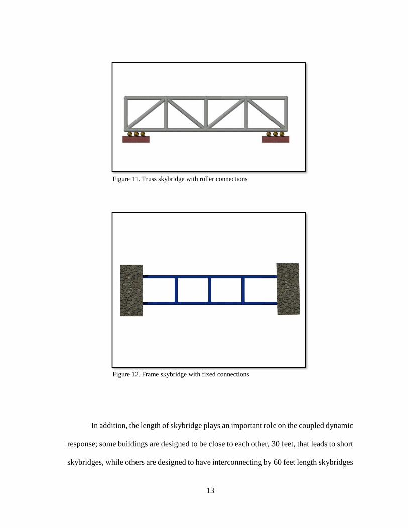
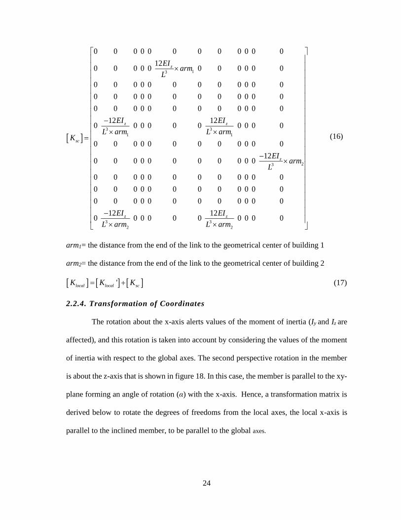
between its ends and the two buildings; the skybridge can be modeled as a truss or frame
as shown in figure 11 and 12 respectively.
Figure 9. Circular Skybridge (Printed from
"The World's Best Photos of skybridge and
way - Flickr Hive Mind", 2017)
Figure 10. Rectangular Skybridge (Printed from
"Skyway or the highway for teaching hospital -
Austin Monitor", 2017)
13
In addition, the length of skybridge plays an important role on the coupled dynamic
response; some buildings are designed to be close to each other, 30 feet, that leads to short
skybridges, while others are designed to have interconnecting by 60 feet length skybridges
Figure 11. Truss skybridge with roller connections
Figure 12. Frame skybridge with fixed connections

14
or longer. When using multiple masses to model the two buildings, it becomes possible to
connect the two buildings by inclined skybridge that connect different floor over the two
buildings, which cannot be represented using a single mass.
The coupled dynamic response of linked high-rise buildings can also be calculated
by using a single mass or multiple masses to model each building in the system by taking
into account the effect of the structural coupling between the dynamic degrees of freedom.
Figure 13 and 14 show the geometrical properties and the dynamic degrees of freedom of
linked high-rise buildings respectively.
Figure 13. Two linked high-rise buildings

15
Using multiple masses to model each building enables us to accurately simulate
systems of two high-rise buildings connected by multiple skybridges as shown in figure
6. Moreover, when using a single mass to model a building in a system of coupled
buildings with a height ratio (Ly1/Ly2) relatively big -not close to one- concentrating the
mass at the geometrical center of the buildings and connecting them by a horizontal
skybridge is impossible. Whereas, by using multiple masses, different height ratios are
considered (1-2).
Figure 14. Dynamic degrees of freedom for two linked buildings

16
2.2. General Matrix Formulation
For a 6-DOF model, such as those shown in figure 8 and figure14, the generalized
displacement vector is of the form,
T
i i i i xi zi yiu w v (1)
The generalized velocity and acceleration vectors can be obtained directly by
differentiating the generalized displacement vector with respect to time. It follows then
that the generalized velocity vector is
T
i i i i xi zi yiu w v (2)
And the generalized acceleration vector is
T
i i i i xi zi yiu w v (3)
2.2.1. Inertial Force
The inertia force can be expressed as
mF M (4)
Where {Fm} is the inertia force vector, [M] is the mass and mass moment of
inertia matrix, and {�̈�} is the dynamic acceleration vector.
For two lumped masses connected by a frame member as shown in figure 15, the
inertia force is
1 2
T
mF F F (5)
1 1 1 1 1 1 1 1 1 1 1 1 1x z yF m u m w m v m m m (6)

17
or
1 1 1 1 1 1 1x z y x z yF Pm Pm Pm Mm Mm Mm (7)
2 2 2 2 2 2 2x z y x z yF Pm Pm Pm Mm Mm Mm (8)
And the corresponding mass matrix is
1
1
1
1
1
1
2
2
2
2
2
2
mx
mz
my
mx
mz
my
m
m
m
I
I zeros
IM
m
zeros m
m
I
I
I
(9)
Figure 15. Two linked lumped masses

18
It is clear that [M] is a diagonal matrix, accordingly, it is applicable whether the
member connecting between the mass is parallel to the global axes or not. The mass matrix
is mapped to the mass matrix of the whole system [Msys].
11
22
0 0 0 0
0 0 0 0
0 0 0 0
0 0 0 0
0 0 0 0
ii
sys
jj
nn
m
m
mM
m
m
(10)
Where n is the number of the lumped masses which are used to represent the
whole system. Hence, the generalized inertia force can be expressed as,
m sys sys sysF M (11)
2.2.2. Elastic Force
In general, there are three types of rigidities in any structural element. These are
axial (EA), flexural (EI), and torsional (GJ) rigidity. Where (E) is the elastic modulus, (G)
shear modulus, (A) is the cross-sectional area, (I) is the moment of inertia, and (J) is the
polar moment of inertia. Each rigidity induces a stiffness that corresponds to a certain
axial, shear, moment, or torsional force. Due to the equilibrium in structures, force
components are coupled. For example, shear and moments in a structural member are
coupled and affected by each other. This requires a stiffness matrix that covers all

19
structural couplings in a structural member subjected to all perspective external loads as
indicated in figure 16. Assumptions were used to simplify the problems as listed below:
1. The material of the members is isotropic and homogenous.
2. The Modulus of Elasticity (E) is the same for tension and compression.
3. The transverse sections remain plane after bending.
Figure 16. Free body diagram of a frame member in a 3D-space along x-axis

20
These forces are connected to the corresponding translational and rotational
displacements as shown below.
sF K (12)
Where {Fs} is the stiffness force vector, [K] is a stiffness matrix and {δ} is the
dynamic displacement vector.
12 1 1 1 1 1 1 2 2 2 2 2 2
T
x z y x z y x z y x z yFs Ps Ps Ps Ms Ms Ms Ps Ps Ps Ms Ms Ms (13)
12 1 1 1 1 1 1 2 2 2 2 2 2
T
x z y x z yu w v u w v (14)

21
(15)
3
3
2
2
3 2 3
3 2 3
2 2
2
120
120 0
0 0 0
6 40 0 0
6 40 0 0 0
'
0 0 0 0 0
12 6 120 0 0 0 0
12 6 120 0 0 0 0 0
0 0 0 0 0 0 0 0
6 2 6 40 0 0 0 0 0 0
6 20 0 0 0
z
y
Symmetric
y y
z z
local
Z z z
y y y
y y y y
z z
EA
L
EI
L
EI
L
GJ
L
EI EI
L L
EI EI
L LK
EA EA
L L
EI EI EI
L L L
EI EI EI
L L L
GJ GJ
L L
EI EI EI EI
L L L L
EI EI
L L
2
6 40 0 0 0z zEI EI
L L

22
The above stiffness matrix is applicable to a member that is parallel to the x-axis.
In order to make the stiffness matrix applicable to any member in the 3D-space, rotations
about the three global axes must be considered as will be discussed later. Since this
stiffness matrix is used to present a model of two high-rise buildings, not a frame, an
additional coupling has to be considered due to the geometrical condition. A skybridge
that connects two high-rise buildings is not linking the centers of the buildings. It connects
the close sides of the two buildings. Accordingly, the distance from the center of the
building to the end of the skybridge forms an arm of the z-translational component,
causing a moment in the building about its y-axis as indicated in figure 17. Hence, the
dynamic response of the building system necessarily impacted in the translational x-
direction and rotational y-direction mainly and the other components indirectly. The
inclusion of this effect has not been considered in prior work into coupled buildings
modeled using a lumped-mass approach. As such, this modeling coupling effect is termed
“Shape Coupling” in this research” and presents an enhancement over prior models for
coupled buildings.

23
2.2.3. Skybridge Considerations
The effect of shape coupling is taken into account by adding the equivalent
moment of the difference of the translational z-component displacements at the ends of
the skybridge multiplied by the corresponding skybridge stiffness. The induced force
causes a torsional force with an arm equals a half of the width of each building. On the
other side, the torsional component in each building causes a translational force on the
connected end of the skybridge.
Figure 17. Shape coupling in coupled buildings
24
(16)
arm1= the distance from the end of the link to the geometrical center of building 1
arm2= the distance from the end of the link to the geometrical center of building 2
'local local scK K K (17)
2.2.4. Transformation of Coordinates
The rotation about the x-axis alerts values of the moment of inertia (Iy and Iz are
affected), and this rotation is taken into account by considering the values of the moment
of inertia with respect to the global axes. The second perspective rotation in the member
is about the z-axis that is shown in figure 18. In this case, the member is parallel to the xy-
plane forming an angle of rotation (α) with the x-axis. Hence, a transformation matrix is
derived below to rotate the degrees of freedoms from the local axes, the local x-axis is
parallel to the inclined member, to be parallel to the global axes.
13
3 3
1 1
23
3
2
0 0 0 0 0 0 0 0 0 0 0 0
120 0 0 0 0 0 0 0 0 0 0
0 0 0 0 0 0 0 0 0 0 0 0
0 0 0 0 0 0 0 0 0 0 0 0
0 0 0 0 0 0 0 0 0 0 0 0
12 120 0 0 0 0 0 0 0 0 0
0 0 0 0 0 0 0 0 0 0 0 0
120 0 0 0 0 0 0 0 0 0 0
0 0 0 0 0 0 0 0 0 0 0 0
0 0 0 0 0 0 0 0 0 0 0 0
0 0 0 0 0 0 0 0 0 0 0 0
120 0 0 0 0
z
z z
sc
z
z
EIarm
L
EI EI
L arm L armK
EIarm
L
EI
L arm
3
2
120 0 0 0 0zEI
L arm

25
local z sFs R F (18)
local zR (19)
Then
1 1
z local z localR Fs K R
(20)
or
1
local z z localFs R K R
(21)
but
local local localFs K (22)
then
Figure 18. Free body diagram of a frame member in a 3D-space with an angle of rotation (α)

26
1
local z zK R K R
(23)
or
1
z local zK R K R
(24)
hence
1
s z local zF R K R
(25)
where
z
z
z
z
z
r
rR
r
r
(26)
and
cos sin 0
sin cos 0
0 0 1
zr
(27)
Another perspective rotation is presented by rotating the member about the global
y-axis; the member is parallel to xz-plane and having an angle of rotation (β) with the
global x-axis as shown in figure 19. The same procedure of (α) rotation is applied to (β);
equation 44 is obtained.
1
y local yK R K R
(28)
or
1
s y local yF R K R
(29)

27
where
y
y
y
y
y
r
rR
r
r
(30)
and
cos 0 sin
0 1 0
sin 0 cos
yr
(31)
Figure 19. Free body diagram of a frame member in a 3D-space with an angle of rotation (β)

28
By considering the combined effect of (α) and (β), the stiffness matrix is obtained
as illustrated below.
1 1
s y z local z yF R R K R R
(32)
and
1 1
y z local z yK R R K R R
(33)
or
1 1
zy local zy yz local yzK R K R R K R
(34)
where
zy z yR R R (35)
yz y zR R R (36)
zy
zy
zy
zy
zy
r
rR
r
r
(37)
cos cos sin cos sin
sin cos cos sin sin
sin 0 cos
zyr
(38)
[K] Is mapped to the stiffness matrix of the whole system (n-MDOF lumped
masses). Let [Kij] be the stiffness matrix for a member connecting between i-th and j-th
joints in the MDOF system.

29
1
_ij zy ij local zyK R K R
(39)
Then
1,1 1,6 1,7 1,12
6,1 6,6 6,7 6,12
7,1 7,6 7,7 7,12
12,1 12,6 12,7 12,12
ij
k k k k
k k k kK
k k k k
k k k k
(40)
Note: the general forms of calculating the elements of the matrix above are listed in the
appendix.
ij ii ij ij
ij
ij ji ij jj
k kK
k k
(41)
The way to map [Kij] to the general stiffness matrix of a structural system of n-
MDOF lumped masses is as shown in the general stiffness matrix of the whole system.
ij ii ij ij
sys
ij ji ij jj
k kK
k k
(42)

30
2.2.5. Damping Force
The generalized damping force can be expressed as
.
sF C (43)
. . . . . .
1 2
T
sys i j n
(44)
Rayleigh Damping was used to calculate the damping force matrix [Csys] of the
system, depending on the mass and stiffness matrices of the whole system.
0 1sys sys sys sys sysC a M a K (45)
where
{asys0} is the mass proportional Rayleigh damping coefficient matrix.
{asys1} is the stiffness proportional Rayleigh damping coefficient matrix.
Both {asys0} and {asys1} are calculated depending on the low natural frequencies
of each component of response by using Matlab.

31
3. MATLAB CODE VALIDATION
The Matlab code that was developed was designed to perform the analysis of a
large DOF with linkage for multiple skybridges. The focus of the research study is to
investigate the dynamic response of high-rise building systems with 1 to 6 skybridges. The
Matlab code enables us to analyze systems of two high-rise buildings (twin or different).
This Matlab code calculates natural frequencies for various force components, considering
the structural coupling and their related modal shapes. A number of verification models
were analyzed and the results were compared with those obtained by using SAP2000.
Table 1 provides information on the number of lumped masses in each building and the
number and locations of skybridges that are used to connect them.
Table 1. Verification models
Model Number of stories
(B1)
Number of stories
(B2)
Linked
stories Comments
1 1 1 1 VM1
2 2 2 1&2
3 2 2 1
4 2 2 2 VM2
5 2 1 1
6 3 3 1&2&3
7 3 3 1
8 3 3 3
9 3 1 1
10 10 10 5&10
11 10 6 5 VM3

32
3.1. Verification Model One (VM1)
This model is the first pass model representing two identical buildings, each
modeled by a single mass, that are linked by a skybridge shown in figure 20. The height
of the vertical members is 120 in, and the values of the equivalent spring flexural rigidity
(EI) and torsional rigidity (GJ) are 133.33×10⁶ lb.in2 and 112.8×10⁶ lb.in2 respectively.
The value of mass is 6.47 kip.sec2/in4. The horizontal frame member has a length of 120
in with axial and flexural rigidities equal to 4×10⁶ lb and 133.33×10⁶ lb.in2 respectively.
Figure 20. Verification model one (VM1)

33
The verification model one (VM1) was also modeled by a 2D portal frame with
lumped masses connected by frame members using SAP2000. The modal properties and
dynamic response that are corresponding to the two horizontal dynamic displacements and
torsional displacement were considered. As we can see in table 2, the natural frequencies
obtained from the Matlab coding are almost the same as those obtained from SAP2000.
The maximum error value is 1%.
Table 2. Natural frequencies for verification model one (VM1)
Verification Model Number One (VM1)
Mode shape Natural frequency (Hz) Error (%)
SAP2000 Matlab 100S M SF F F
1 1.90 1.90 0.00
2 16.27 16.27 0.00
3 1.90 1.90 0.00
4 2.13 2.11 0.70
Table 3 provides information on the modal shapes for the Matlab and SAP2000
solutions, and it can be seen that they are also very close. These results, as a first
verification model, indicate that the effects of structural coupling are correctly considered
in the equations of motion regarding the linked high-rise buildings.

34
Table 3. Mode shapes for verification model one (VM1)
Verification Model Number One (VM1)
mode shape (1)
mas
s
SAP2000 Matlab
trans (x) trans (z) rot (y) trans (x) trans (z) rot (y)
1 1 0 1 0 0
2 1 0 1 0 0
mode shape (2)
mas
s
SAP2000 Matlab
trans (x) trans (z) rot (y) trans (x) trans (z) rot (y)
1 1 0 0 1 0 0
2 -1 0 0 -1 0 0
mode shape (3)
mas
s
SAP2000 Matlab
trans (x) trans (z) rot (y) trans (x) trans (z) rot (y)
1 0 1 0 0 1 0
2 0 1 0 0 1 0
mode shape (4)
mas
s
SAP2000 Matlab
trans (x) trans (z) rot (y) trans (x) trans (z) rot (y)
1 0 1 -0.0146 0 1 -0.0148
2 0 -1 -0.0146 0 -1 -0.0148
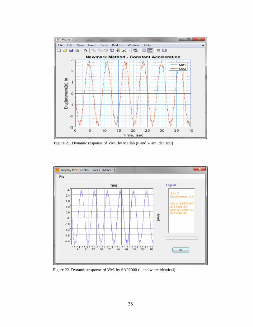
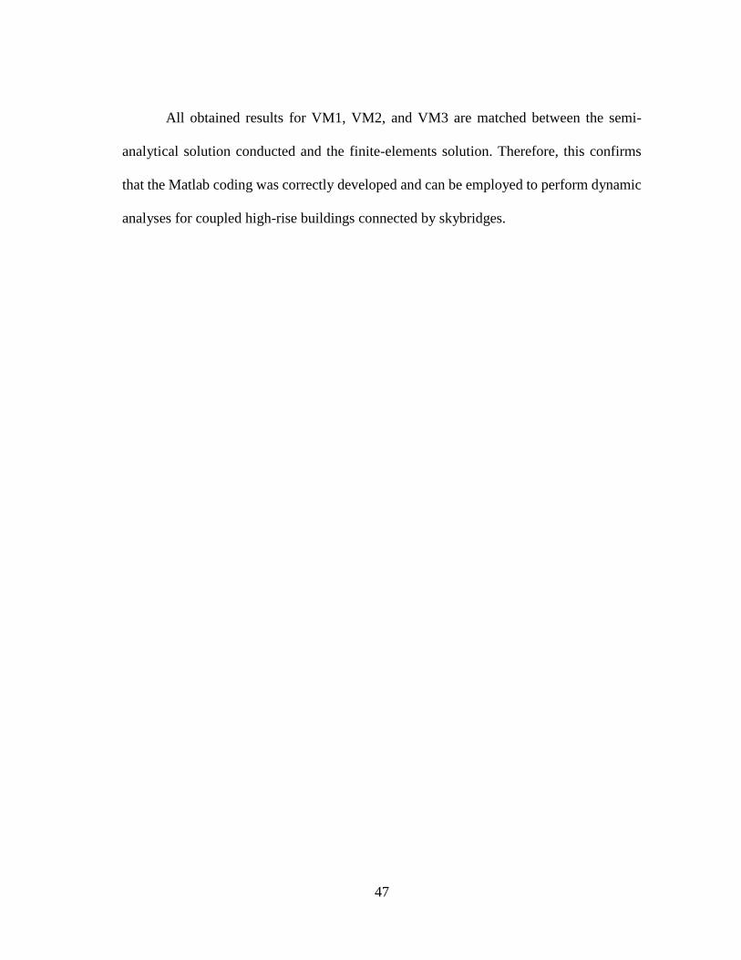
Sine wave dynamic loading was applied to both Matlab and SAP2000 models.
Figure 21 and 22 show the dynamic response of both of the two masses in the VM1 in the
x-direction. It is the same as the z-direction. Figure 20 was obtained from the Matlab
solution, whereas figure 21 was obtained from SAP2000. Accordingly, all previous results
for VM1 refer to that the Matlab coding was generated correctly.
35
Figure 21. Dynamic response of VM1 by Matlab (u and w are identical)
Figure 22. Dynamic response of VM1by SAP2000 (u and w are identical)

36
3.2. Verification Model Two (VM2)
The second verification model is similar to the first verification model (VM1) in
all dynamic and geometrical properties. However, in this case, it has a total of four lumped
masses, two per building, as shown in figure 23. VM2 has significantly more changes in
the numerical solution steps as a result of the existence of a vertical coupling between
lumped masses in addition to the horizontal coupling due to the links. As shown in table
4 and table 5 the modal shapes and the corresponding frequencies obtained from Matlab
and SAP2000 match.
Figure 23. Verification model two (VM2)

37
Table 4. Mode shapes for verification model two (MV2)
Verification Model Number Two (VM2)
mode shape (1)
mass SAP2000 Matlab
trans (x) trans (z) rot (y) trans (x) trans (z) rot (y)
1 0.618 0 0 0.618 0 0
2 1 0 0 1 0 0
3 0.618 0 0 0.618 0 0
4 1 0 0 1 0 0
mode shape (2)
mass SAP2000 Matlab
trans (x) trans (z) rot (y) trans (x) trans (z) rot (y)
1 1 0 0 1 0 0
2 -0.618 0 0 -0.618 0 0
3 1 0 0 1 0 0
4 -0.618 0 0 -0.618 0 0
mode shape (3)
mass SAP2000 Matlab
trans (x) trans (z) rot (y) trans (x) trans (z) rot (y)
1 -0.618 0 0 -0.618 0 0
2 -1 0 0 -1 0 0
3 0.618 0 0 0.618 0 0
4 1 0 0 1 0 0
mode shape (4)
mass SAP2000 Matlab
trans (x) trans (z) rot (y) trans (x) trans (z) rot (y)
1 1 0 0 1 0 0
2 -0.618 0 0 -0.618 0 0
3 -1 0 0 -1 0 0
4 0.618 0 0 0.618 0 0
mode shape (5)
mass SAP2000 Matlab
trans (x) trans (z) rot (y) trans (x) trans (z) rot (y)
1 0 0.618 0 0 0.618 0
2 0 1 0 0 1 0
3 0 0.618 0 0 0.618 0
4 0 1 0 0 1 0

38
Table 4. Continues
mode shape (6)
mass SAP2000 Matlab
trans (x) trans (z) rot (y) trans (x) trans (z) rot (y)
1 0 -0.618 0.0098 0 -0.618 0.0098
2 0 -1 0.0159 0 -1 0.0159
3 0 0.618 0.0098 0 0.618 0.0098
4 0 1 0.0159 0 1 0.0159
mode shape (7)
mass SAP2000 Matlab
trans (x) trans (z) rot (y) trans (x) trans (z) rot (y)
1 0 1 0 0 1 0
2 0 -0.618 0 0 -0.618 0
3 0 1 0 0 1 0
4 0 -0.618 0 0 -0.618 0
mode shape (8)
mass SAP2000 Matlab
trans (x) trans (z) rot (y) trans (x) trans (z) rot (y)
1 0 1 -0.0122 0 1 -
0.0124
2 0 -0.618 0.0075 0 -0.618 0.0077
3 0 -1 -0.0122 0 -1 -
0.0124
4 0 0.618 0.0075 0 0.618 0.0077
Table 5. Natural frequencies for verification model two (VM2)
Verification Model Number Two (VM2)
Mode shape Natural frequency (Hz) Error (%)
SAP2000 Matlab 100S M SF F F
1 1.18 1.18 0.00
2 3.08 3.08 0.00
3 16.20 16.20 0.00
4 16.45 16.45 0.00
5 1.18 1.18 0.00
6 1.32 1.31 0.81
7 3.08 3.08 0.00
8 3.38 3.37 0.49

39
An important question may be raised regarding what is the reason that the natural
frequencies relative to third and fourth modal shapes jumping to much bigger values than
others. This is because that every two lumped masses over the link have opposite
directions, as seen in table 3. Hence, the link is under high tension or compression that
increases the stiffness of the structure leading to higher frequencies due to the additional
axial stiffness of the link itself.
3.3. Verification Model Three (VM3)
Ultimately, VM3 is considered a sophisticated analysis of a complicated model
with sixteen lumped masses, as shown in figure 24. For simplicity, the dynamic properties
used were the same as those in VM1 and VM2. However, the number of lumped masses
were not the same on the two sides of the link. In addition, not all lumped masses were
connected horizontally, instead, some randomness of linking the lumped masses was
achieved in order to determine if the Matlab coding gave the same results of SAP2000.

40
Figure 24. Verification model three (VM3)

41
Table 6. Natural frequencies for VM3
Verification Model Number Two (VM2)
Mode shape Natural frequency (Hz) Error (%)
SAP2000 Matlab 100S M SF F F
1 0.33 0.33 0.01
2 0.74 0.74 0.01
3 1.17 1.17 0.00
4 1.37 1.37 0.00
5 1.65 1.65 0.00
6 2.11 2.11 0.00
8 2.43 2.43 0.00
7 2.23 2.23 0.00
9 2.82 2.82 0.00
10 3.08 3.08 0.00
11 3.17 3.17 0.00
12 3.41 3.41 0.00
13 3.62 3.62 0.00
14 3.64 3.64 0.00
15 3.73 3.73 0.00
16 16.38 16.38 0.00
17 0.30 0.30 0.14
18 0.49 0.48 0.62
19 0.85 0.85 0.31
20 1.35 1.35 0.20
21 1.39 1.39 0.21
22 1.91 1.88 1.31
23 2.16 2.17 0.09
24 2.37 2.38 0.04
25 2.79 2.79 0.09
26 2.85 2.85 0.16
27 3.15 3.15 0.02
28 3.38 3.36 0.49
29 3.43 3.42 0.26
30 3.64 3.64 0.01
31 3.70 3.69 0.29
32 3.77 3.75 0.35

42
As we can see in table 6, the maximum difference in the natural frequencies
between the Matlab and SAP2000 solutions is 2%, which is very acceptable. The dynamic
response of two lumped masses (m10 and m14) in the model was drawn in order to compare
them. Three degrees of freedom were examined, which are the translational displacement
in the x and z directions and the torsional displacements about the y-axis. Figure 25
through figure 30 show the three components of the dynamic displacements which
calculated by Matlab code and SAP2000.
Figure 25. Horizontal displacement (u) at m10 and m14 of VM3 by Matlab

43
Figure 26. Horizontal displacement (u) at m10 and m14 of VM3 by SAP2000
Figure 27. Horizontal displacement (w) at m10 and m14 of VM3 by Matlab

44
Figure 28. Horizontal displacement (w) at m10 and m14 of VM3 by SAP2000
Figure 29. Torsional displacement (y) at m10 and m14 of VM3 by Matlab

45
The first two modal shapes of the dynamic displacement along x-axis and z-axis
by Matlab are shown in figure 31 and 32 respectively.
Figure 30. Torsional displacement (y) at m10 and m14 of VM3 by SAP2000

46
Figure 31. First two modes in x-direction for VM3 by Matlab
Figure 32. First two modes in coupled y-direction for VM3 by Matlab
47
All obtained results for VM1, VM2, and VM3 are matched between the semi-
analytical solution conducted and the finite-elements solution. Therefore, this confirms
that the Matlab coding was correctly developed and can be employed to perform dynamic
analyses for coupled high-rise buildings connected by skybridges.

48
4. ISOLATED AND COUPLED HIGH-RISE BUILDING
SIMULATIONS
4.1. Undamped Twin High-rise Building System
This chapter investigates the effect of utilizing the single and multiple masses in
the building modeling with respect to the analysis of the high-rise buildings connected by
a skybridge. Based on this reason, a system of ‘two twins,’ is considered, as indicated in
figure 4. The acronym, HBS1 is used to express (High-rise Building system 1) for
simplicity. For illustrative purposes the height of the building was selected to be 210 feet,
corresponding to a 15-story building. The top view of the two buildings is a square-shaped
plan form whose structural properties are shown in table 7 below. The total number of the
columns in each floor is 25.
Table 7. Structural Properties of B1 and B2 in High-rise building system 1 (HBS1)
Story 1-5 6-10 11-15
Column dimensions (ft) 4 × 4 3× 3 2 × 2
Column height (ft) 14 14 14
Number of columns per story 25 25 25
Beam dimensions (ft) 2 × 1.5 2 × 1.5 2 × 1.5
Slab thickness (in) 8 8 8

49
The dynamic degrees of freedom considered for the two scenarios included the
translation along the x-axis and z-axis directions and the torsional degree of freedom about
the y-axis. In addition, the dynamic response of the system was calculated for the case of
the independent building response, a skybridge was not present, while the case of the twin
buildings is interconnected at the eighteenth and nineteenth floors by a skybridge 50 feet
in length. The dynamic properties of the skybridge link are shown in table 8.
Table 8. Structural Properties of the Skybridge in HBS1
Section shape Length (ft) A × Ec (kips) Iz × Ec (kips.in2)
rectangular 50 53856000 214×109
Two modeling scenarios were considered. The first scenario considered the use of
the multiple masses, specifically fifteen lumped masses were used to model each building.
In the second scenario, the mass of each building was concentrated at the geometrical
center of each building as a single mass for each building, resulting in two lumped masses
for the entire system. Following that, the structural models of the high-rise buildings were
subjected to a strong ground motion relative to the loading time series records selected
from an event of the 1940 El-Centro earthquake in the United States, see the appendix for
more details.

50
The obtained dynamic response of the highest point in the ΗSB1 (m15) by the first
modeling scenario shows that the maximum dynamic displacement of about 10” occurred
the twenty-sixth second. Whereas the maximum dynamic displacement of the same point
in this particular building, which was gotten from the second scenario of the analysis is
about 10” at the fourteenth second. For these two scenarios, the dynamic responses along
the x-axis and z-axis are identical because of the absence of the structural coupling.
Figures 33 and 34 show the dynamic response of the first and second modeling scenarios
respectively.
Figure 33. Horizontal displacement (u) at m15 (H=210 feet) in HBS1 using Multiple masses

51
Several tests were conducted by changing the height of the equivalent mass so as
to ensure the best modeling approximation of the second scenario is achieved to converge
to the solution gotten by the first scenario, which is modestly more illustrative of the real
dynamic response. The location of the equivalent mass was inserted in the sixth, tenth,
and fifteenth floor, considering the change of the equivalent stiffness and damping. The
dynamic response under the 1940 El-Centro earthquake was further calculated for each
case and the results are shown in figure 35 through figure 38. The general indication is the
increase in the natural frequency and the decrease in the dynamic response, when the
equivalent lumped mass is kept in the location closest to the first floor and vice versa, and
also, when the equivalent lumped mass is kept close to the highest floor in the buildings.
Figure 34. Horizontal displacement (u) at m15 (H=210 feet) in HBS1 using a single mass
concentrated at 8th floor

52
Figure 36. Horizontal displacement (u) at m15 (H=210 feet) in HBS1 using a single mass
concentrated at 10th floor
Figure 35. Horizontal displacement (u) at m15 (H=210 feet) in HBS1 using a single mass
concentrated at 6th floor

53
Figure 38. Horizontal displacement (u) at m15 (H=210 feet) in HBS1 using a single mass
concentrated at 15th floor
Figure 37. Horizontal displacement (u) at m15 (H=210 feet) in HBS1 using a single mass
concentrated at 12th floor
54
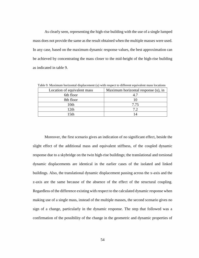
As clearly seen, representing the high-rise building with the use of a single lumped
mass does not provide the same as the result obtained when the multiple masses were used.
In any case, based on the maximum dynamic response values, the best approximation can
be achieved by concentrating the mass closer to the mid-height of the high-rise building
as indicated in table 9.
Table 9. Maximum horizontal displacement (u) with respect to different equivalent mass locations
Location of equivalent mass Maximum horizontal response (u), in
6th floor 4.7
8th floor 10
10th 7.75
12th 7.2
15th 14
Moreover, the first scenario gives an indication of no significant effect, beside the
slight effect of the additional mass and equivalent stiffness, of the coupled dynamic
response due to a skybridge on the twin high-rise buildings; the translational and torsional
dynamic displacements are identical in the earlier cases of the isolated and linked
buildings. Also, the translational dynamic displacement passing across the x-axis and the
z-axis are the same because of the absence of the effect of the structural coupling.
Regardless of the difference existing with respect to the calculated dynamic response when
making use of a single mass, instead of the multiple masses, the second scenario gives no
sign of a change, particularly in the dynamic response. The step that followed was a
confirmation of the possibility of the change in the geometric and dynamic properties of

55
the skybridge makes any possible change or not. The study makes use of different
skybridge models as indicated in table 10.
Table 10. Different dynamic characteristics of the skybridge in HBS1
Section shape Length (ft) Location A × Ec (kips) Iz × Ec (kips.in2)
rectangular 60 15th -16th 60000000 300 ×109
rectangular 50 10th -11th 50000000 250 ×109
rectangular 40 6th -7th 45000000 200 ×109
rectangular 30 3rd -4th 30000000 150 ×109
All of the obtained results give a confirmation that the presence of the skybridge
in this system; that is, the twin high buildings, has no significant effect of structural
coupling on the dynamic response. Hence, it is possible to conclude that there exists no
structural coupling in twin high-rise building, being interconnected by a skybridge
subjected to viable ground motions.
4.2. Undamped Different High-rise Building Systems
Different high-rise building systems are considered for the coming sections of this
research study. The high-rise building system 2 (HBS2) is another building system
considered in this study. It has its first building in 20 stories, having 280 feet in height.
However, the second one has 10 stories and is 140 feet in height. The geometrical
properties of the first and second high-rise buildings are indicated in table 11 and 12
respectively.
56
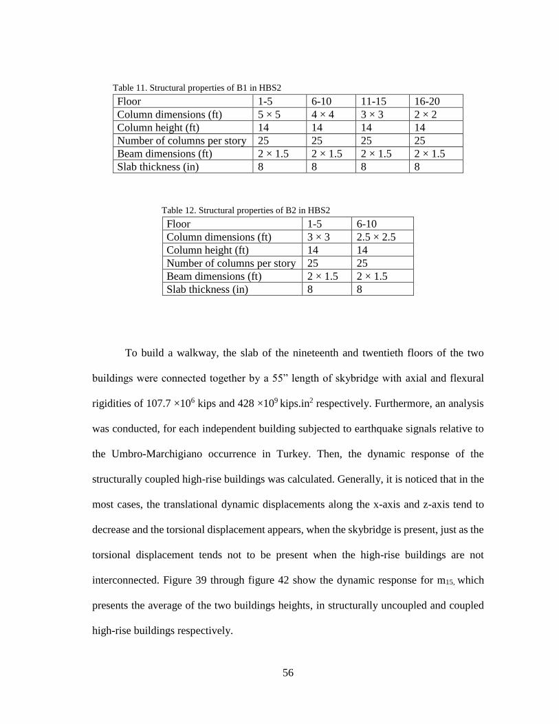
Table 11. Structural properties of B1 in HBS2
Floor 1-5 6-10 11-15 16-20
Column dimensions (ft) 5 × 5 4 × 4 3 × 3 2 × 2
Column height (ft) 14 14 14 14
Number of columns per story 25 25 25 25
Beam dimensions (ft) 2 × 1.5 2 × 1.5 2 × 1.5 2 × 1.5
Slab thickness (in) 8 8 8 8
Table 12. Structural properties of B2 in HBS2
Floor 1-5 6-10
Column dimensions (ft) 3 × 3 2.5 × 2.5
Column height (ft) 14 14
Number of columns per story 25 25
Beam dimensions (ft) 2 × 1.5 2 × 1.5
Slab thickness (in) 8 8
To build a walkway, the slab of the nineteenth and twentieth floors of the two
buildings were connected together by a 55” length of skybridge with axial and flexural
rigidities of 107.7 ×10⁶ kips and 428 ×109 kips.in2 respectively. Furthermore, an analysis
was conducted, for each independent building subjected to earthquake signals relative to
the Umbro-Marchigiano occurrence in Turkey. Then, the dynamic response of the
structurally coupled high-rise buildings was calculated. Generally, it is noticed that in the
most cases, the translational dynamic displacements along the x-axis and z-axis tend to
decrease and the torsional displacement appears, when the skybridge is present, just as the
torsional displacement tends not to be present when the high-rise buildings are not
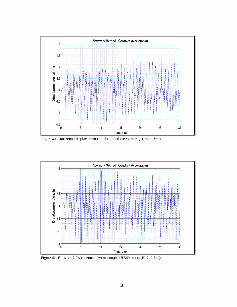
interconnected. Figure 39 through figure 42 show the dynamic response for m15, which
presents the average of the two buildings heights, in structurally uncoupled and coupled
high-rise buildings respectively.

57
Figure 39. Horizontal displacement (u) of uncoupled HBS2 at m15 (H=210 feet)
Figure 40. Horizontal displacement (w) of uncoupled HBS2 at m15 (H=210 feet)
58
Figure 41. Horizontal displacement (u) of coupled HBS2 at m15 (H=210 feet)
Figure 42. Horizontal displacement (w) of coupled HBS2 at m15 (H=210 feet)

59
4.3. Damped Different High-Rise Building System
HSB2 was utilized to determine the impact of damping force in this section of
the thesis. The dynamic displacement was obtained relative to the different value of
damping ratio, represented by
𝜉 = 0.02, 0.035, 0.05, 0.065, 0.08, 0.1
Furthermore, the proportional viscous damping matrices were constructed with the
use of Rayleigh damping, considering the same damping ratios for the first two modes.
Figure 43 and figure 44 show the dynamic response of coupled HBS2 with damping ratio
equals 0.02 at m15, and figure 45 shows the maximum dynamic displacement passing
across the z-axis in the system’s top floor, at the twentieth second, on the y-axis, and the
damping ratio of the x-axis. The two curves indicate that more energy dissipated in the
case of uncoupled buildings under the effect of the damping force.
Figure 43. Horizontal displacement (u) of coupled HBS2 at m15 (H=210 feet), (x=0.02)

60
Figure 45. Change of horizontal displacement (wmax) at m20 (H=280 feet) with the damping ratio
Figure 44. Horizontal displacement (w) of coupled HBS2 at m15 (H=210 feet),(x=0.02)

61
Finally, the relationship between the required number of cycles for the dynamic
horizontal displacement w, along the z-axis, to drop to 10% of the wmax as well as the
damping ratio is also represented in figure 46. The number of cycles decreases when the
damping ratio increases and vice versa.
Figure 46. Change of the number of cycles for horizontal displacement (w) at m20 (H=280 feet) to
drop to (10%) of the maximum value relative to the damping ratio

62
5. MULTIPLE SKYBRIDGE SIMULATIONS
This chapter will focus on the investigation of the geometrical and dynamic
properties and their effect on the dynamic response of the coupled high-rise building
system. In particular, we will examine the variation of the response behavior subject to
variations in skybridge stiffness, location, connection end conditions and the number of
skybridges used to connect the high-rise buildings. In order to further observe and
understand the response behavior, two different high-rise building systems are
considered.
5.1. Skybridge Connection End Conditions
Although different connection end conditions may be utilized in the structural
design to link a skybridge to the high-rise buildings, the appropriate connection design
must be compatible with the type of skybridge structural design. For example, if the
structural designer is inclined to eliminate the effect of the structural coupling on the
building system dynamic response resulting from the skybridge linkage they would use a
roller design for the skybridge end connections. This is the simplest case to model as only
the additional relatively small mass of the skybridge need be is taken into account.
Linking the ends of the skybridge using hinge-supports induces a coupled dynamic
response of the building system. Hinge end connections develop a resistance against the
translational degree of freedom along the x-axis, parallel to the skybridge, and this leads
to the structural coupling to the corresponding dynamic degree of freedom (u). Any
resistance of the translational degree of freedom along the z-axis effects the corresponding

63
dynamic degree of freedom (w). As can be noted in the formulation of stiffness matrix,
presented in chapter two, (u) is not coupled with (w) or ( 𝜃𝑦) whether the skybridge linkage
exists or not.
The 1994 Northridge earthquake event was applied to get the dynamic
displacements for uncoupled roller design and the coupled hinge-supported skybridge of
HBS3 respectively. The geometrical properties of building one denoted by the symbol B1
and building two denoted by the symbol B2 are shown in tables 13 and 14 respectively.
Table 13. Structural properties of B1 in HSB3
Floor 1-10 11-20
Column dimensions (ft) 5 × 5 4 × 4
Column height (ft) 14 14
Number of columns per story 25 25
Beam dimensions (ft) 2 × 1.5 2 × 1.5
Slab thickness (in) 8 8
Table 14. Structural properties of B2 in HSB3
Floor 1-8 9-14
Column dimensions (ft) 4 × 4 3.5 × 3.5
Column height (ft) 14 14
Number of columns per story 25 25
Beam dimensions (ft) 2 × 1.5 2 × 1.5
Slab thickness (in) 8 8 .
64
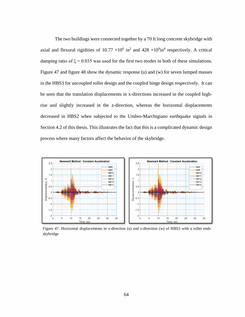
The two buildings were connected together by a 70 ft long concrete skybridge with
axial and flexural rigidities of 10.77 ×10⁶ in2 and 428 ×109in4 respectively. A critical
damping ratio of ξ = 0.035 was used for the first two modes in both of these simulations.
Figure 47 and figure 48 show the dynamic response (u) and (w) for seven lumped masses
in the HBS3 for uncoupled roller design and the coupled hinge design respectively. It can
be seen that the translation displacements in x-directions increased in the coupled high-
rise and slightly increased in the z-direction, whereas the horizontal displacements
decreased in HBS2 when subjected to the Umbro-Marchigiano earthquake signals in
Section 4.2 of this thesis. This illustrates the fact that this is a complicated dynamic design
process where many factors affect the behavior of the skybridge.
Figure 47. Horizontal displacements in x-direction (u) and z-direction (w) of HBS3 with a roller ends
skybridge

65
Following that, a resistance against the rotational degree of freedom ( 𝜃𝑦) was
introduced to model fixed end conditions of the skybridge. That modification significantly
increased the effect of the skybridge by increasing the horizontal dynamic displacement
in the z-direction (w). Thus, the hinge support design increased the dynamic displacement
(w) slightly and, the introduction of rotational resistance in the fixed support design further
increased this effect. Moreover, the rotational constraint introduced a torsional
displacement of buildings about their local vertical axes as shown in figure 49.
Figure 48. Horizontal displacements in x-direction (u) and z-direction (w) of HBS3 with a hinge ends
skybridge

66
5.2. Skybridge Stiffness
The high-rise building system 4 (HBS4) was linked by a 44 ft long skybridge. The
effect of variable skybridge structural stiffness was investigated by changing the
equivalent cross-sectional area of the skybridge. This was done in, in order to evaluate the
effect of different stiffnesses on the dynamic response, where the axial and flexural stiffens
increase by increasing the equivalent cross-sectional area of the skybridge and vice versa.
The geometrical properties of the two different buildings are presented in table 15 and
table 16.
Table 15. Geometrical properties of B1 in HSB4
Floor 1-10 11-22
Column dimensions (ft) 5 × 5 4 × 4
Column height (ft) 14 14
Number of columns per story 25 25
Beam dimensions (ft) 2 × 1.5 2 × 1.5
Slab thickness (in) 8 8
Figure 49. Dynamic displacements (u) and (w) of HSB3 with a fixed ends skybridge

67
Table 16. Geometrical properties of B2 in HSB4
Floor 1-8 9-12
Column dimensions (ft) 4 × 4 3.5 × 3.5
Column height (ft) 14 14
Number of columns per story 25 25
Beam dimensions (ft) 2 × 1.5 2 × 1.5
A fixed ended skybridge design was used to connect the tenth floor between the
two buildings. The axial and flexural rigidities of the skybridge are 53.85 ×10⁶ kips and
214 ×109 kips.in2 respectively. The normalized axial rigidity and flexural rigidity that is
based on these a cross-area and the moments of inertia are set to be 1.
A critical damping ratio of ξ = 0.035 was used in these simulations. The uncoupled
dynamic response of HBS4 is denoted by (u1) and (w1). Hence, different values of the
translational and rotational stiffness of the skybridge were considered and their
corresponding displacements were calculated. It is worth mentioning that the change of
the stiffness covers the change of the skybridge shape, the material used to build it, and
the length. The artificial NF17 earthquake signals were applied in this part of the study
with maximum acceleration 10g and time step 0.01 sec. figure 50 and figure 51 show the
impact of different values of normalized rigidities, divided by the axial and flexural
rigidity values that were set to be 1, on the dynamic displacements for the twenty-second
floor of B1 (mt) and eighteenth floor of B2 (ms).
Note:
mt= the mass of 20th floor in the taller building
ms = the mass of 10th floor in the shorter building

68
Figure 50. Change of horizontal displacement (u) of mt (H=308 feet) and ms (H=154 feet) at the
twenty-second floor with change of the normalized axial rigidity
Figure 51. Change of horizontal displacement (w) of mt (H=308 feet) and ms (H=154 feet) with
change of the normalized flexural rigidity

69
As shown in figure 49, the optimum normalized axial stiffness that reduces the
overall dynamic displacement along the x-axis (u) for the two buildings is (1/4). Where
figure 50 indicates that the normalized flexural stiffness (1) is the optimum value that
achieved the minimum value of the overall dynamic displacement along the z-axis (w).
The two horizontal displacements (u) and (w) are uncoupled and impacted by different
components of frame rigidities; that is why the normalized optimum rigidities are not the
same. For this reason, the shape of a skybridge shall be designed to have high flexural
rigidity and low axial rigidity values.
5.3. Location of a Skybridge
The high-rise building system 4 (HBS4) was used again with different elevations
specified for the skybridges. The dynamic displacement along the x-axis and z-axis were
calculated in each case. Figure 52 and figure 53 show the maximum dynamic displacement
across the number of floors where the skybridge set. The optimum values of axial and
flexural stiffness that are obtained from the previous section were utilized. It is clear that
tenth floor 83% of the height of shorter buildings (B2) is the optimum position where the
skybridge shall be set.
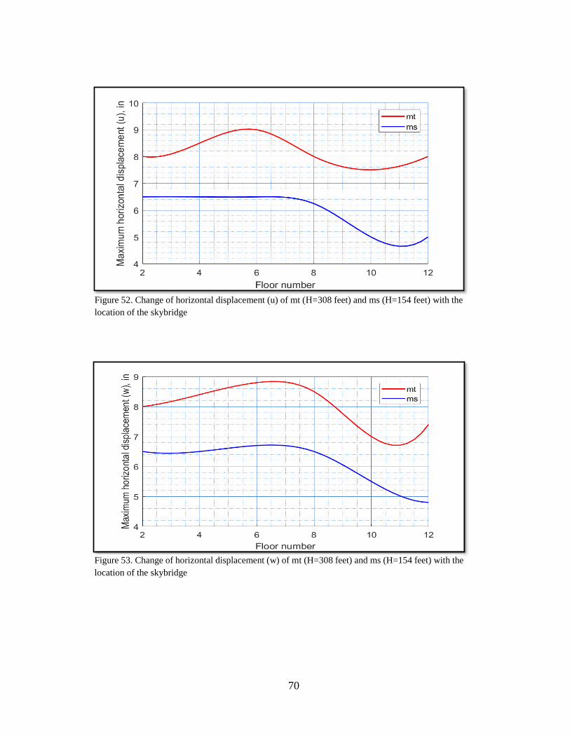
70
Figure 53. Change of horizontal displacement (w) of mt (H=308 feet) and ms (H=154 feet) with the
location of the skybridge
Figure 52. Change of horizontal displacement (u) of mt (H=308 feet) and ms (H=154 feet) with the
location of the skybridge

71
5.4. Number of Skybridges
In this section, the number of skybridges that are specified to connect the two high-
rise buildings is varied in order to minimize the dynamic displacement response as much
as possible. The damped high-rise building system (HBS4) that was used in Sections 5.2
& 5.3 is used again in these simulations. The same values of the optimum axial and rigid
stiffness are used again. The dynamic response was calculated relative to different number
of skybridges represented by,
N=1, 2, 3, 4, 5, 6
The results obtained from the previous part of this section (Section 5.3) were
employed to determine the location of these skybridges. Therefore, the first one was set to
be on the tenth floor, the first optimum location of a skybridge. When using two
skybridges, the second on was put on the twelfth floor, the second optimum location of a
skybridge. Table 17 introduced the number of skybridges and their locations.
Table 17. Number of skybridges and their locations
N Floor
1 10
2 10& 12
3 2& 10& 12
4 2& 8& 10& 12
5 2& 4& 8& 10& 12
6 2& 4& 6& 8&1 0& 12

72
The variation of the maximum dynamic displacements as a function of the number
of skybridges (N) is shown in figure 54 and figure 55. The specification of one skybridge
results in the minimum dynamic displacement along the two directions in the higher
building (B1), whereas the specification of two skybridges minimizes the dynamic
displacement of the shorter building (B2).
Figure 54. Change of horizontal displacement (u) of mt (H=308 feet) and ms (H=154 feet) with
number of skybridges (N)

73
Figure 56 illustrates the change in the natural frequencies relative to the first four
modal shapes of the x-direction motion with respect to the number of skybridges used to
connect the buildings. The modal shapes that have a big displacement difference over the
two masses that are connected by the skybridges usually witness significant changes in
their corresponding natural frequencies.
Figure 55. Change of horizontal displacement (w) of mt (H=308 feet) and ms (H=154 feet) with
number of skybridges (N)

74
5.5. Statistical Characterization of the Excitation and Response
Another perspective from which to investigate the structural coupling of high-rise
buildings linked by skybridges involves the statistical characterization of both the strong
ground motion excitation and the structural response to that excitation. Herein the mean,
standard deviation, skewness, and kurtosis were evaluated for the four strong ground
motion time series used in this research study and the resulting building system response.
The skewness and kurtosis provide a measure of the deviation of these time series from
Gaussian processes. Note that for a Gaussian process the skewness and kurtosis would
have values of zero and three respectively. Information on each of the four earthquake
Figure 56. Change of natural frequencies of x-direction with N

75
measurements and their statistical characteristics are presented in Table 18. Here one can
observe the non-Gaussian nature of each of the earthquake time series.
Table 18. Statistical analysis of earthquake records
Strong ground
motion records Δt (sec)
Duration
(sec)
Max
a/g
Statistical characteristics
mean std skewness kurtosis
1940 El-Centro 0.02 50 0.342 ~0 0.0477 0.447 11.01
1994 Northridge 0.02 60 0.273 ~0 0.5452 -1.269 68.64
Umbro Marchigiano 0.01 30 0.455 ~0 0.5432 0.340 26.55
NF17 - artificial 0.01 5 10.61 ~0 1.219 2.176 31.11
The dominant frequencies that are significantly higher than others in each of the
time series records were evaluated using a Fast Fourier Transformation (FFT), and the
results are listed in Table19.
Table 19. The dominant frequencies of earthquake records
Strong ground motion record Dominant frequencies (rad/sec)
1940 El-Centro 7.28; 9.17; 13.57
1994 Northridge 2.72; 27.64
Umbro Marchigiano 39.86; 42.71; 45.11
NF17 73.99; 81.52; 90.3; 107.9
The 1940 El-Centro and 1994 Northridge earthquakes were used to excite the two
high-rise building system (HBS5) whose geometrical properties are listed for B1 and B2
in table 20 and 21 respectively.

76
Table 20. Geometrical Properties of B1 in HBS5
Story 1-10 11-15
Column dimensions (ft) 4 × 4 3 × 3
Column height (ft) 14 14
Slab thickness (in) 8 8
Table 21. Geometrical properties of B2 in HBS5
Story 1-8 9-12
Column dimensions (ft) 3 × 3 2 × 2
Column height (ft) 14 14
Slab thickness (in) 8 8
Two cases were investigated where first the buildings were linked by a single
skybridge and then by three skybridges. The characteristics of the skybridges are
presented in Table 22.
Table 22. Geometrical properties of the skybridge in HBS5
Section shape Length (ft) A × Ec (kips) Iz (in4)
rectangular 55 26925000 214×109
Two different critical damping ratios (ξ = 0.01, 0.1) were applied to the building
systems in order to observe their behavior of the system under different loadings, numbers
of skybridges, and damping. Table 23 and Table 24 summarize the statistical
characterization of the resulting response behavior.
Next, we consider the use of histograms to visualize the response behavior of the
highest point on the shorter building and this is presented in Figures 57 through 60. The
decrement in the standard deviation values and the increment in the absolute values of the

77
kurtosis when the damping ratio goes from 0.01 to 0.1 can be interpreted as the overall
dynamic response over the whole period of the earthquake is reduced. On the other hand,
when using three skybridges to connect the two buildings instead of one, the value of
standard deviation decreases and the absolute values of skewness and kurtosis increase,
and this gives an indication of the same positive impact of using multiple skybridges.
However, in the case of high manufactured damping (0.1), the effect of the existence of
three skybridges (verse one skybridges) is not significant due to fast dissipation in the
energy of the building system.

78
Table 23. Statistical characterization of HBS5 response subjected to the 1940 El-Centro record
The 1940 El-Centro
Number of
skybridges Damping ratio Direction Mean (in)
SD (in) Skewness Kurtosis
min max min max min max
1
0.01
xt ~0 0.15 2.05 -0.01 0.02 3.56 3.83
zt ~0 0.00 1.74 -0.03 0.14 1.87 3.73
yr ~0 0.00 0.00 - - - -
0.1
xt ~0 0.04 0.59 -0.30 0.06 8.75 9.04
zt ~0 0.00 0.81 -0.08 0.39 6.35 8.87
yr ~0 0.00 0.00 - - - -
3
0.01
xt ~0 0.14 1.85 -0.10 0.03 4.49 4.67
zt ~0 0.00 1.74 -0.03 0.14 1.87 3.74
yr ~0 0.00 0.00 - - - -
0.1
xt ~0 0.05 0.56 -0.34 0.06 8.80 9.04
zt ~0 0.00 0.81 -0.08 0.39 6.37 8.86
yr ~0 0.00 0.00 - - - -

79
Table 24. Statistical characterization of HBS5 response subjected to the 1994 Northridge record
The 1994 Northridge
Number of
skybridges
Damping
ratio Direction Mean(in)
SD(in) Skewness Kurtosis
min max min max min max
1
0.01
xt ~0 0.06 0.79 -0.11 0.12 3.05 7.70
zt ~0 0.00 2.85 -0.07 0.28 2.96 7.51
yr ~0 0.00 0.00 - - - -
0.1
xt ~0 0.03 0.34 -0.15 1.12 8.65 11.96
zt ~0 0.00 0.63 0.06 0.96 7.92 12.48
yr ~0 0.00 0.00 - - - -
3
0.01
xt ~0 0.06 0.78 -0.08 0.19 2.79 3.97
zt ~0 0.00 2.83 -0.06 0.28 2.97 7.50
yr ~0 0.00 0.00 - - - -
0.1
xt ~0 0.03 0.32 -0.09 1.19 8.46 11.26
zt ~0 0.00 0.62 0.06 0.97 7.94 12.47
yr ~0 0.00 0.00 - - - -

80
Figure 58. Normal distribution of (u) with three skybridges (El-Centro)
Figure 57. Normal distribution of (u) with a skybridge (El-Centro)
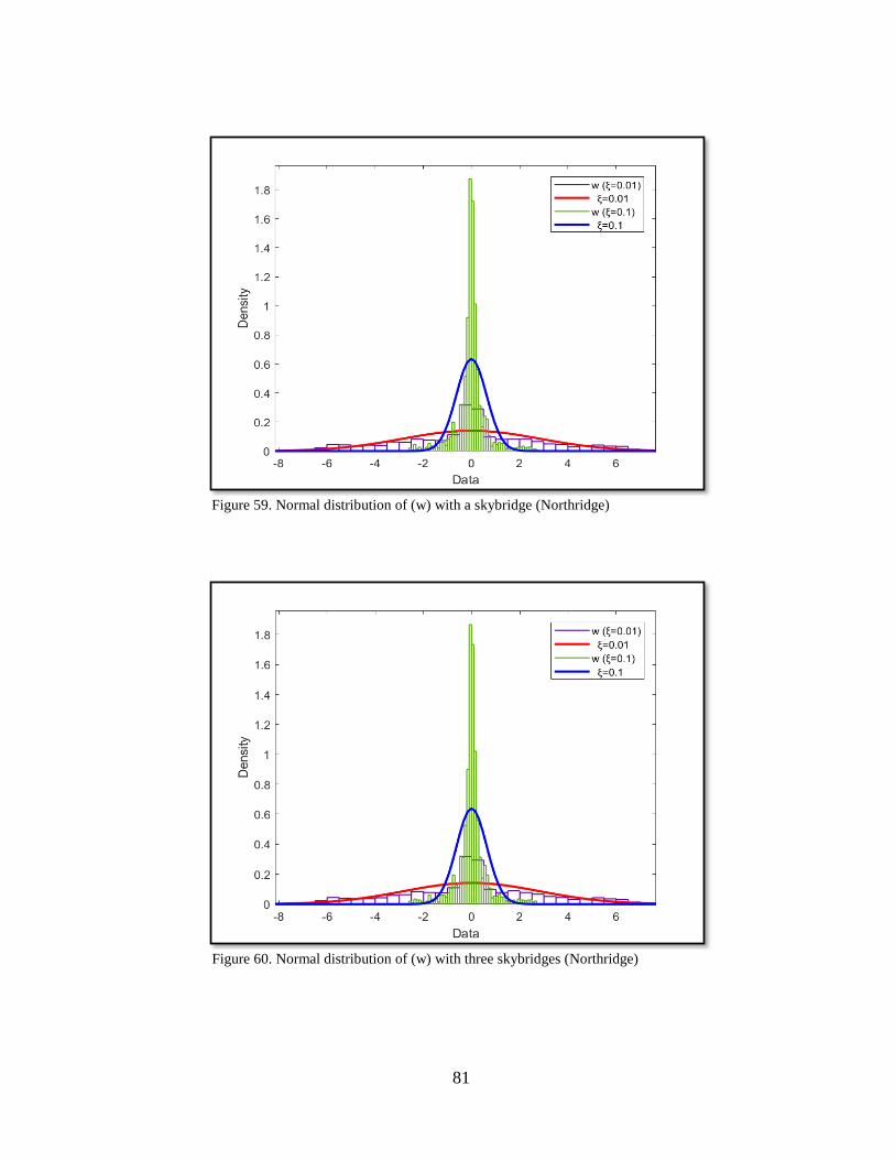
81
Figure 59. Normal distribution of (w) with a skybridge (Northridge)
Figure 60. Normal distribution of (w) with three skybridges (Northridge)

82
6. SUMMARY AND CONCLUSIONS
This study presented a structural model that focused on the dynamic response of
adjacent buildings connected at one or more elevations by skybridges. The frame based
multi-degree-of-freedom model utilized allowed for the inclusion of both translational and
rotational degrees of freedom. The focus of the illustrative examples was the modeling of
high-rise buildings of different story height that were linked by one or more skybridges.
The building systems were subjected to earthquake loads.
A review previous relevant research studies allowed the identification of
knowledge gaps that guided this research investigation. It was found that three earlier
studies directly addressed the structural coupling of twin buildings coupled by a single
skybridge. Lim, Bienkiewicz, & Richards (2011), examined the response of a coupled
twin high-rise building system subjected to wind loading. Their model assumed a single
lumped mass for each building that was allowed to have multiple degrees of freedom
(MDOF). The three-degree of freedom models allowed for translation in the inline and
transverse directions, as well as rotation around the vertical axis. Lee, Kim, & Ko (2012)
utilized a finite element model and were able to consider lead rubber bearings and linear
motion bearings to model the connection between the skybridge and the two high-rise
buildings subjected to wind and earthquake loads. Their study focused on the simulation
of translational degrees of freedom. Later in the study by Song and Tse (2014), they
considered the effect of wind loads where they modeled each building using a series of
lumped masses, one at each floor elevation.

83
Consequently, a more general formulation that could address translational and
rotational degrees of freedom for buildings of different plan form and elevation, and single
or multiple skywalks was developed in this research study. The resulting formulation
was implemented in Matlab and validated using SAP2000. Due to the complexity of the
structural system, a Newmark-Beta time integration model was used to solve for the
dynamic response behavior. Eleven building systems with different geometries and
dynamic properties using were investigated and it was found that the predicted results
using the 3-D frame formulation resulted in an error on the order of less than 2%.
The nine building systems that were the focus of this research investigation was
the nine cases identified in Table 25, which is repeated here for clarity. A total of 51
numerical simulations were systematically analyzed and documented in this thesis. The
system parameters varied in these simulations included: building height, number of
skybridges, their elevation and connectivity boundary conditions, lumped sum mass
characteristics, story stiffness, and system damping. The role of critical damping ratios in
modifying the structural response behavior was investigated. For very lightly damped
systems a range of 1-3% was assumed and a value of 10% that might result from
manufactured damping was briefly investigated. A statistical analysis characterizing the
nature of four different earthquakes and the corresponding structural system response
behavior was performed.

84
Table 25. Case studies that were considered in this research study
Case
Number Case Description
Number
of Runs Variation
1
Single lumped
mass model for twin
buildings
5 Concentrating the lumped mass in
different locations
2
Multiple lumped
mass model for twin
buildings
5 Height and properties of the
skybridge
3
Multiple lumped
mass model for
different buildings
2 Coupled (with a skybridge) and
uncoupled.
4
Multiple lumped mass
model
for non-conservative
different buildings
7 Damping ratio (0 to 10%)
5
Multiple lumped
mass model for
different buildings
3
Supporting condition of the
skybridge ends:
Roller, hinge, and fixed
6
Multiple lumped mass
model
for non-conservative
different buildings
9 Stiffness of the skybridge
7
Multiple lumped mass
model
for non-conservative
different buildings
6 Height of the skybridge
8
Multiple lumped mass
model
for non-conservative
different buildings
6 Number of skybridges (1 to 6)
9
Multiple lumped mass
model
for non-conservative
different buildings
8 Statistical characterization

85
The central conclusions of this research study based on the numerical simulations
of adjacent buildings with an unequal number of stories connected by one or more
skybridges are as follows:
1. The introduction of skybridges to connect adjacent buildings can significantly
impact the mode shapes and natural frequency estimates and dynamic response
behavior.
2. The introduction of multiple skybridge connections impacts the higher modes and
has a significant impact on the structural system response behavior.
3. The structural system displacement response is modified by the introduction of
skybridges designed with hinged end supports and is also influenced by the
structural characteristics of the skybridge design.
4. The structural system displacement and rotational response behavior is modified
by skybridges designed with fixed ended connections and is also influenced by the
structural characteristics of the skybridge design.
5. It was observed that there are optimum translational stiffness and flexural stiffness
characteristics for skybridge design that would minimize the building system
dynamic response behavior. Further, it was observed that deviations of skybridge
stiffness required to minimize the dynamic response of the shorter building system
is more than that required for a taller building system.
6. For the building systems investigated, it was observed that a single skybridge
located at an elevation of about 80% of the shorter building height would minimize
the dynamic displacement behavior.

86
7. The introduction of a single skybridge reduces the dynamic response of the taller
building, whereas the introduction of two skybridges was observed to minimize
the dynamic response for the shorter building.
8. Based on the numerical simulations it was determined that the best approximation
for the inclusion of a skybridge can be achieved by concentrating its mass
contributions closer to the center of the geometry of each high-rise building.
9. Statistical characterization of the excitation and response behavior illustrated that
non-Gaussian excitation was filtered by the building system to yielding a reduced
non-Gaussian response.
It is clear that further investigation into this challenging structural design problem is
needed to better understand some of the results found in this research study. The analysis
and Matlab code developed, as part of this research study is quite general and can address
skybridge vertical connection between different floors and situations where there is
horizontal miss-alignment of buildings. The idea of optimizing/minimizing the building
system dynamic response is also quite intriguing especially for high-rise buildings that are
located in dense population area where space for building footprints is often quite limited.

87
REFERENCES
Behnamfar, F., Dorafshan, S., Taheri, A., & Hosseini Hashemi, B. (2016). A method for
rapid estimation of dynamic coupling and spectral responses of connected
adjacent structures. The Structural Design of Tall and Special Buildings, 25(13),
605-625.
Chen, X., & Kareem, A. (2005). Dynamic Wind Effects on Buildings with 3D Coupled
Modes: Application of High Frequency Force Balance Measurements. Journal of
Engineering Mechanics, 131(11), 1115-1125.
Chopra, A. K. (2001). Dynamics of structures: theory and applications to earthquake
engineering. 2nd ed. Anil K. Chopra: Upper Saddle River, NJ: Prentice-Hall,
[2001] 2nd ed.
Clough, R. W., & Penzien, J. (2010). Dynamics of structures. 2nd ed., Rev. Ray W. Clough,
Joseph Penzien: Berkeley, Calif. : Computers and Structures, [2010]
2nd ed., Rev.
Klein, R. E., & Healey, M. D. (1987). Semi-Active Control of Wind Induced Oscillations
in Structures. In H. H. E. Leipholz (Ed.), Structural Control: Proceedings of the
Second International Symposium on Structural Control, University of Waterloo,
Ontario, Canada, July 15–17, 1985 (pp. 354-369). Dordrecht: Springer
Netherlands.

88
Le, T.-H., & Caracoglia, L. (2015). Wavelet-Galerkin analysis to study the coupled
dynamic response of a tall building against transient wind loads. Engineering
Structures, 100, 763-778.
Lee, D.-G., Kim, H.-S., & Ko, H. (2012). Evaluation of coupling–control effect of a sky-
bridge for adjacent tall buildings. The Structural Design of Tall and Special
Buildings, 21(5), 311-328.
Lim, J., & Bienkiewicz, B. (2009). Effects of Structural and Aerodynamic Couplings on
the Dynamic Response of Tall Twin Buildings with a Skybridge Structures
Congress 2009 (pp. 1-9).
Lim, J., Bienkiewicz, B., & Richards, E. (2011). Modeling of structural coupling for
assessment of modal properties of twin tall buildings with a skybridge. Journal of
Wind Engineering and Industrial Aerodynamics, 99(5), 615-623.
Lim, J., & University, C. S. (2008). Structural Coupling and Wind-induced Response of
Twin Tall Buildings with a Skybridge: Colorado State University.
Lomholt, I., Lomholt, I., Solkoff, J., & Solkoff, J. (2017). Bahrain World Trade Center:
Manama, BWTC - e-architect. e-architect. Retrieved 28 April 2017, from
https://www.e-architect.co.uk/bahrain/bahrain-world-trade-centre
McCall, A. J., & Balling, R. J. (2016). Structural analysis and optimization of tall buildings
connected with skybridges and atria. Structural and Multidisciplinary
Optimization, 1-18.
Paz, M., & Leigh, W. E. (2004). Structural dynamics: theory and computation. 5th ed.
Mario Paz, William Leigh: Boston: Kluwer Academic Publishers, [2004] 5th ed.

89
Rogers, S. (2017). Sky Bridges: 14 Aerial Structures that Span Skyscrapers. WebUrbanist.
Retrieved 28 April 2017, from http://weburbanist.com/2013/09/16/sky-bridges-
14-aerial-structures-that-span-skyscrapers/2/
Skyway or the highway for teaching hospital - Austin Monitor. (2017). Austin Monitor.
Retrieved28 April 2017, from
https://www.austinmonitor.com/stories/2014/09/skyway-highway-teaching-
hospital/
Song, J., & Tse, K. T. (2014). Dynamic characteristics of wind-excited linked twin
buildings based on a 3-dimensional analytical model. Engineering Structures, 79,
169-181.
The World's Best Photos of skybridge and way - Flickr Hive Mind.
(2017). Hiveminer.com. Retrieved 28 April 2017, from
https://hiveminer.com/Tags/skybridge,way
Zhao, X., Sun, H. H., & Zheng, Y. M. (2009). Identification and updating for the three-
dimensional finite element model of a long span steel skybridge. The Structural
Design of Tall and Special Buildings, 18(6), 625-646.

90
APPENDIX A
STRUCTURAL STIFFNESS MATRIX DEVELOPMENT
The following analysis provides the details used in the development of the
stiffness equations used in equation (40) elements presented in chapter 2 of this thesis:
1 sin( )sin( )f
2 sin( )cos( )f
3 cos( )sin( )f
4 cos( )cos( )f
2 2 2 2 2 2 2 3
1,1 1 1(1 (sin ) (sin ) ) 12 (sin ) 12 ((sin )y zk EAL f EI EI f L
2 3
1,2 2,1 4 sin ( 12 )zk k f EAL EI L
2 2 2 3
1,3 3,1 3 ( (cos ) 12 12 ((cos ) 1)y zk k f EAL EI EI L
2
1,4 4,1 26 sin( )( )y zk k f EI EI L
2
1,5 5,1 36 yk k f EI L
2
1,6 6,1 1 16 sin( ) sin( )(1 )y zk k EI f EI f L
1,7 7,1 1,1k k k
1,8 8,1 1,2k k k
1,9 9,1 1,3k k k

91
1,10 10,1 1,4k k k
1,11 11,1 1,5k k k
1,12 12,1 1,6k k k
2 2 2 3
2,2 12 12 (sin ) (sin )z yk EI EI EAL L
2 3
2,3 3,2 1 cos( )( 12 )zk k f EAL EI L
2
2,4 4,2 36 zk k EI f L
2,5 5,2 0k k
2
2,6 6,2 26 zk k EI f L
2,7 7,2 2,1k k k
2,8 8,2 2,2k k k
2,9 9,2 2,3k k k
2,10 10,2 2,4k k k
2,11 11,2 2,5k k k
2,12 12,2 2,6k k k
2 2 2 2 2 3
33 1 1((sin ) )) 12 (1 (sin ) ) 12y zk EAL f EI EI f L
2 2 2
3,4 4,3 6sin( ) (1 (sin ) ) (sin )y zk k EI EI L
2
3,5 5,3 46 yk k EI f L
2
3,6 6,3 26 sin( )( )y zk k f EI EI L

92
3,7 7,3 3,1k k k
3,8 8,3 3,2k k k
3,9 9,3 3,3k k k
3,10 10,3 3,4k k k
3,11 11,3 3,5k k k
3,12 21,3 3,6k k k
2 2 2 2 2 2
4,4 1 14 ((sin ) ) 4 (sin ) (1 (sin ) (sin ) )y zk EI f EI GJ f L
4,5 5,4 4 sin( )(4 )yk k f EI GJ L
4,6 6,4 sin(2 ) 2 (1 cos(2 )) 4 (1 cos(2 )) 22
y z
GJk k EI EI L
4,7 7,4 4,1k k k
4,8 8,4 4,2k k k
4,9 9,4 4,3k k k
2 2 2 2 2 2
4,10 10,4 1 12 ((sin ) ) 2 (sin ) ( 1 (sin ) (sin ) )y zk k EI f EI GJ f L
4,11 11,4 4 sin( )(2 )yk k f EI GJ L
4,12 12,4 sin(2 ) (cos(2 ) 1) 2 (1 cos(2 )) 22
y z
GJk k EI EI L
2 2
5,5 4 (1 (sin ) ) (sin )yk EI GJ L
5,6 6,5 3 sin( ) (4 )yk k f EI GJ L

93
5,7 7,5 5,1k k k
5,8 8,5 0k k
5,9 9,5 5,3k k k
5,10 10,5 4 sin( )(2 )yk k f EI GJ L
2 2
5,11 11,5 2 ((sin ) 1) (sin )yk k EI GJ L
5,12 12,5 3 sin( ) (2 )yk k f EI GJ L
2 2 2 2
6,6 1 14 4 (1 (sin ) ) ( (sin ) )y zk f EI EI GJ f L
6,7 7,6 6,1k k k
6,8 8,6 6,2k k k
6,9 9,6 6,3k k k
6,10 10,6 sin(2 ) 2 ( 1 cos(2 )) 2 (1 cos(2 )) 22
y z
GJk k EI EI L
6,11 11,6 3 sin( ) (2 )yk k f EI GJ L
2 2 2 2
6,12 12,6 1 12 2 (1 (sin ) ) ( (sin ) )y zk k f EI EI GJ f L
7,7 7,1k k
7,8 8,7 7,2k k k
7,9 9,7 7,3k k k
7,10 10,7 7,4k k k

94
7,11 11,7 7,5k k k
7,12 12,7 7,6k k k
8,8 8,2k k
8,9 9,8 8,3k k k
8,10 10,8 8,4k k k
8,11 11,8 0k k
8,12 12,8 8,6k k k
9,9 9,3k k
9,10 10,9 9,4k k k
9,11 11,9 9,5k k k
9,12 21,9 9,6k k k
10,10 4,4k k
10,11 11,10 4 sin( ) (4 )yk k f EI GJ L
10,12 12,10 sin(2 ) 2 (1 cos(2 )) 4 (1 cos(2 )) 22
y z
GJk k EI EI L
2 2
11,11 4 (1 (sin ) ) (sin )yk EI GJ L
12,11 11,12 3 sin( ) (4 )yk k f EI GJ L
2 2 2 2
12,12 1 14 4 (1 (sin ) ) ( (sin ) )y zk f EI EI GJ f L

95
APPENDIX B
EARTHQUAKE RECORDS
Figure 61. The 1940 El-Centro earthquake record

96
Figure 62. The 1940 El-Centro power spectral density
Figure 63. The 1994 Northridge earthquake record

97
Figure 65. The Umbro-Marchigiano earthquake record
Figure 64. The 1994 Northridge power spectral density

98
Figure 67. The artificial NF-17 earthquake record
Figure 66. The Umbro-Marchigiano power spectral density

99
Figure 68. The artificial NF-17 power spectral density