Strong SH-to-Love Wave Scattering off the SouthernCalifornia Continental BorderlandChunquan Yu1 , Zhongwen Zhan1 , Egill Hauksson1 , and Elizabeth S. Cochran2

1Seismological Laboratory, California Institute of Technology, Pasadena, CA, USA, 2Earthquake Science Center, U.S.Geological Survey, Pasadena, CA, USA

Abstract Seismic scattering is commonly observed and results from wave propagation in heterogeneousmedium. Yet deterministic characterization of scatterers associated with lateral heterogeneities remainschallenging. In this study, we analyze broadband waveforms recorded by the Southern California SeismicNetwork and observe strongly scattered Love waves following the arrival of teleseismic SH wave. Thesescattered Love waves travel approximately in the same (azimuthal) direction as the incident SH wave at adominant period of ~10 s but at an apparent velocity of ~3.6 km/s as compared to the ~11 km/s for the SHwave.Back projection suggests that this strong scattering is associated with pronounced bathymetric relief in theSouthern California Continental Borderland, in particular the Patton Escarpment. Finite-difference simulationsusing a simplified 2-D bathymetric and crustal model are able to predict the arrival times and amplitudes ofmajor scatterers. The modeling suggests a relatively low shear wave velocity in the Continental Borderland.

1. Introduction

The Earth to the first order can be characterized as radially symmetric medium. Such “1-D” reference Earthmod-els, such as ak135, can predict phase arrival times within an accuracy of a few seconds (Kennett et al., 1995). Thecommon observations of seismic scattering indicate that heterogeneities are also ubiquitous throughout theEarth (see Sato et al., 2012; Shearer, 2007 for reviews). Since the 1970s, there have been numerous theoreticaland observational efforts intended to investigate the relationship between seismic scattering and heteroge-neous structures of the Earth. Many earlier studies treated the scattering process in a stochastic way that onlyallowed for statistical description of the heterogeneity (e.g., Aki, 1969; Sato et al., 2012; Shearer, 2007; Wu, 1985).The reasons a stochastic approach has primarily been used are twofold. First, in many cases heterogeneitieswithin the Earth are randomly distributed and scattered energy due to individual scatterers is weak. Second,the density of seismic recordings is often too sparse to locate individual scatterers.

Strong lateral heterogeneities in seismic wave velocity or density, such as bathymetric/topographic relief,basin edges, and fault zone structures, are potentially strong scatterers. Forward simulations suggest thattopography can have a significant effect on seismic wave propagation, including scattering of body andsurface waves and (de)amplification of peak ground velocities (e.g., Geli et al., 1988; Lee et al., 2009).Similarly, basin edges can also generate surface waves and cause large amplification of ground motions(e.g., Frankel, 1993; Graves et al., 1998). In addition, strong lateral gradient in seismic anisotropy can also resultin surface wave mode scattering, such as observations of quasi-Love waves (Park & Yu, 1993). Studying thesestrongly scattered waves thus not only helps us better understand Earth’s heterogeneous/anisotropic struc-tures but also is useful for assessing seismic hazard, including the calibration and refinement of regionalseismic velocity models used to locate earthquakes and simulate strong ground motions.

With the recent growth of seismic arrays, deterministic characterization of seismic scatterers has becomefeasible. Meanwhile, the development of array processing and migration techniques (e.g., AlTheyab et al.,2016; Berkhout, 1982; Rost & Thomas, 2002) allows for improved identification and location of scatterers.For example, Spudich and Bostwick (1987) applied array analysis to an earthquake cluster to locate scatterersnear the earthquake focal region. Using P-to-P scattering, Revenaugh (1995) demonstrated that in the uppermantle strong scatterers are located near the southern flank of the remnant slab beneath the TransverseRanges. Multipath Rayleigh waves are also reported along the West Coast of North America (Ji et al., 2005)and are interpreted as reflections off roots of the Rocky Mountains.

A special case of seismic scattering involves body-to-surface wave conversion. By analyzing three-componentseismic waveforms as recorded by the NORESS array in southern Norway; Bannister et al. (1990) detected

YU ET AL. S. CALIFORNIA SH-TO-LOVE SCATTERING 10,208

PUBLICATIONSGeophysical Research Letters

RESEARCH LETTER10.1002/2017GL075213

Key Points:• Strong SH-to-Love wave scattering isobserved by the Southern CaliforniaSeismic Network

• Back projection suggests that strongscatterers are associated withpronounced bathymetric relief in theContinental Borderland

• Two-dimensional finite-differencesimulations predict the arrival timesand amplitudes of scattered Lovewaves

Supporting Information:• Supporting Information S1

Correspondence to:C. Yu,yucq@gps.caltech.edu

Citation:Yu, C., Zhan, Z., Hauksson, E., &Cochran, E. S. (2017). Strong SH-to-Lovewave scattering off the SouthernCalifornia continental borderland.Geophysical Research Letters, 44,10,208–10,215. https://doi.org/10.1002/2017GL075213

Received 6 AUG 2017Accepted 29 AUG 2017Accepted article online 21 SEP 2017Published online 21 OCT 2017

©2017. American Geophysical Union.All Rights Reserved.

strongly scattered Rayleigh waves in the teleseismic P wave coda and determined that scatterers locate totwo nearby areas with pronounced topographic relief. Furumura et al. (1998) observed large-amplitudeRayleigh and Love waves from deep earthquakes at regional distances. Their back projection and syntheticwaveform modeling suggest that scatterers are located close to the Norfolk Ridge where crustal structurehas strong lateral heterogeneity. More recently, Maeda et al. (2014) analyzed Japan Hi-net data and founda scattered wave train following the P wave arrival of a teleseismic event. They attributed the scattered wavetrain to reverberations in the seawater near the Japan Trench.

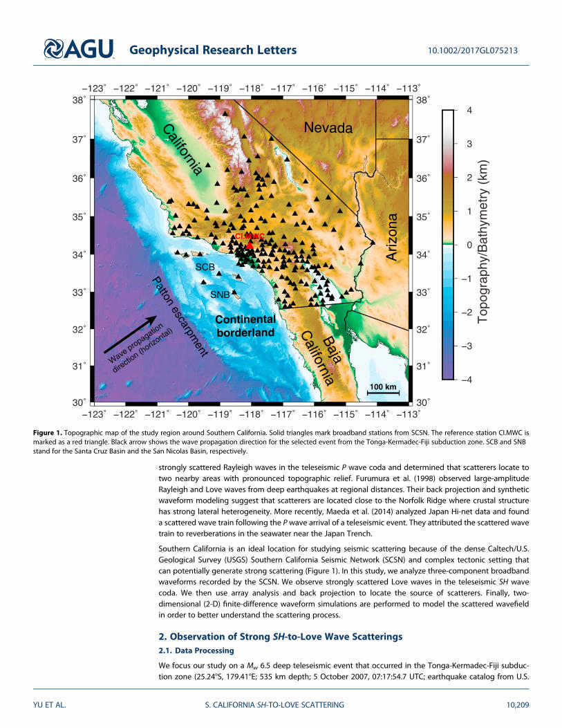
Southern California is an ideal location for studying seismic scattering because of the dense Caltech/U.S.Geological Survey (USGS) Southern California Seismic Network (SCSN) and complex tectonic setting thatcan potentially generate strong scattering (Figure 1). In this study, we analyze three-component broadbandwaveforms recorded by the SCSN. We observe strongly scattered Love waves in the teleseismic SH wavecoda. We then use array analysis and back projection to locate the source of scatterers. Finally, two-dimensional (2-D) finite-difference waveform simulations are performed to model the scattered wavefieldin order to better understand the scattering process.

2. Observation of Strong SH-to-Love Wave Scatterings2.1. Data Processing

We focus our study on a Mw 6.5 deep teleseismic event that occurred in the Tonga-Kermadec-Fiji subduc-tion zone (25.24°S, 179.41°E; 535 km depth; 5 October 2007, 07:17:54.7 UTC; earthquake catalog from U.S.

Top

ogra

phy/

Bat

hym

etry

(km

)

California

Nevada

anozirA

Patton escarpment

Continentalborderland

Wave propagatio

n

directi

on (horiz

ontal)

SCB

SNB

CI.MWCB

aja

California

100 km

Figure 1. Topographic map of the study region around Southern California. Solid triangles mark broadband stations from SCSN. The reference station CI.MWC ismarked as a red triangle. Black arrow shows the wave propagation direction for the selected event from the Tonga-Kermadec-Fiji subduction zone. SCB and SNBstand for the Santa Cruz Basin and the San Nicolas Basin, respectively.

Geophysical Research Letters 10.1002/2017GL075213

YU ET AL. S. CALIFORNIA SH-TO-LOVE SCATTERING 10,209

National Earthquake Information Center). We collected three-component broadband seismic waveformsfrom SCSN (Figure 1). We then cut seismograms using a time window that begins 200 s before andends 600 s after the expected S wave arrival time, estimated using the ak135 velocity model (Kennettet al., 1995). After rotating seismograms into vertical, radial, and transverse components, we furtherapply a two-pass Butterworth filter between 0.02 and 0.1 Hz to suppress the background microseisms.Seismograms are visually checked using the Crazyseismic software (Yu et al., 2017), and traces with lowsignal-to-noise ratio are removed. Finally, amplitudes are normalized by the maximum peak of theincident SH wave.

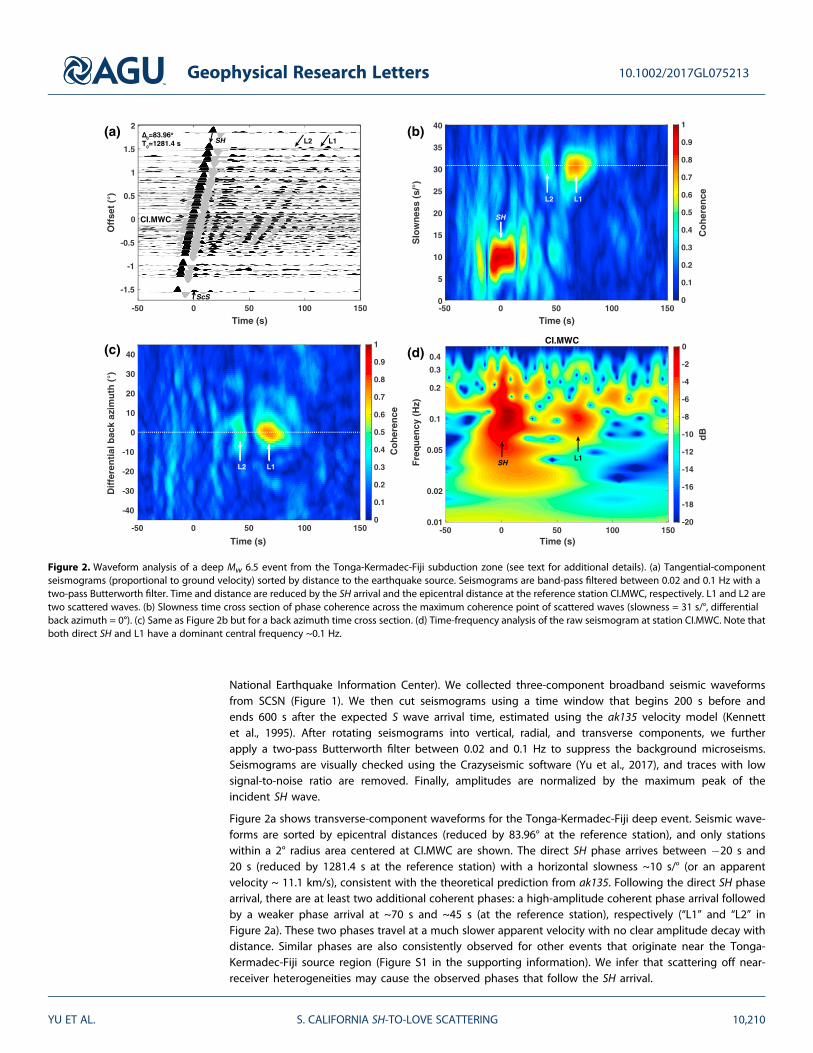
Figure 2a shows transverse-component waveforms for the Tonga-Kermadec-Fiji deep event. Seismic wave-forms are sorted by epicentral distances (reduced by 83.96° at the reference station), and only stationswithin a 2° radius area centered at CI.MWC are shown. The direct SH phase arrives between �20 s and20 s (reduced by 1281.4 s at the reference station) with a horizontal slowness ~10 s/° (or an apparentvelocity ~ 11.1 km/s), consistent with the theoretical prediction from ak135. Following the direct SH phasearrival, there are at least two additional coherent phases: a high-amplitude coherent phase arrival followedby a weaker phase arrival at ~70 s and ~45 s (at the reference station), respectively (“L1” and “L2” inFigure 2a). These two phases travel at a much slower apparent velocity with no clear amplitude decay withdistance. Similar phases are also consistently observed for other events that originate near the Tonga-Kermadec-Fiji source region (Figure S1 in the supporting information). We infer that scattering off near-receiver heterogeneities may cause the observed phases that follow the SH arrival.

-50 0 50 100 150

Time (s)

-1.5

-1

-0.5

0

0.5

1

1.5

2

Off

set

(°)

SH0

-50 0 50 100 150

Time (s)

0

5

10

15

20

25

30

35

40

Slo

wn

ess

(s/°

)

0

0.1

0.2

0.3

0.4

0.5

0.6

0.7

0.8

0.9

1

Co

her

ence

-50 0 50 100 150

Time (s)

-40

-30

-20

-10

0

10

20

30

40

Dif

fere

nti

al b

ack

azim

uth

(°)

0

0.1

0.2

0.3

0.4

0.5

0.6

0.7

0.8

0.9

1

Co

her

ence

-50 0 50 100 150Time (s)

0.01

0.02

0.05

0.1

0.2

0.3

0.4

Fre

qu

ency

(H

z)

CI.MWC

-20

-18

-16

-14

-12

-10

-8

-6

-4

-2

0

dB

(a) (b)

(c) (d)

Figure 2. Waveform analysis of a deep Mw 6.5 event from the Tonga-Kermadec-Fiji subduction zone (see text for additional details). (a) Tangential-componentseismograms (proportional to ground velocity) sorted by distance to the earthquake source. Seismograms are band-pass filtered between 0.02 and 0.1 Hz with atwo-pass Butterworth filter. Time and distance are reduced by the SH arrival and the epicentral distance at the reference station CI.MWC, respectively. L1 and L2 aretwo scattered waves. (b) Slowness time cross section of phase coherence across the maximum coherence point of scattered waves (slowness = 31 s/°, differentialback azimuth = 0°). (c) Same as Figure 2b but for a back azimuth time cross section. (d) Time-frequency analysis of the raw seismogram at station CI.MWC. Note thatboth direct SH and L1 have a dominant central frequency ~0.1 Hz.

Geophysical Research Letters 10.1002/2017GL075213

YU ET AL. S. CALIFORNIA SH-TO-LOVE SCATTERING 10,210

2.2. Array Analysis: Phase Coherence

We apply array analysis to estimate the propagation direction, slowness, and arrival time of each of the strongscattered arrivals. In particular, we rely on the phase coherence (or phase stack) method of Schimmel andPaulssen (1997). Phase coherence detects coherent signals based on the instantaneous phase. Real seismictraces are first converted to analytic traces by applying a Hilbert transform. The amplitudes of analytic tracesare normalized to unity. Phase coherence c(t) is then constructed by a summation of analytic traces in thecomplex plane (Schimmel & Paulssen, 1997), that is,

c tð Þ ¼ 1N

XN

j¼1

eiΦ j tð Þ�����

����� (1)

where N is the number of traces and Φj(t) the instantaneous phase of the jth trace. Since amplitudes arenormalized, the value of phase coherence always ranges between 0 and 1. An advantage of this method isits ability to detect weak coherent signals, making it well suited for studying seismic scattering.

Figures 2b and 2c show phase coherence measurements along two cross sections with preferred backazimuth and slowness of the strongest scatter, respectively. Scattered waves L1 and L2 propagate in thesame azimuthal direction as the incident SH wave. However, their large horizontal slowness ~31 s/°indicates that they travel at a much slower apparent velocity (~3.6 km/s) than the incident SH wave(Figures 2b and 2c). Time-frequency analysis (Stockwell et al., 1996) of the raw seismic waveform recordedat station CI.MWC shows that scattered waves have a dominant central frequency of ~0.1 Hz, similar tothat of the incident SH wave (Figure 2d). We note that our waveform analysis is stable over various fre-quency bandwidths, albeit with a higher noise level if filtered with a higher cutoff frequency, such asat 0.2 Hz.

While an apparent velocity of 3.6 km/s is too slow to correspond to a teleseismic body wave arrival, the velo-city is consistent with a ~10 s period Love wave or a horizontally traveling SHwave in the crust. Although it isnot possible to distinguish Love waves and SHwaves based on particle motions, the lack of clear decay in theamplitude of scattered waves (Figure 2a) and our 2-D finite-difference simulations (see section 4) bothsuggest that the scattered waves are Love waves. We note that the scattered Love waves are relatively narrowband and have no clear evidence of dispersion (Figure 2d).

3. Locations of Scatterers

We use back projection to locate the sources of scattered Love waves. The apparent source wavelet (includ-ing the primary SH and its depth phases), obtained using principal component analysis (Jolliffe, 2002), issubtracted and deconvolved from each trace. Residual traces are then shifted and stacked in a 1° radiusbin around each station for all back azimuths, assuming a constant horizontal slowness 31 s/° (estimated fromthe entire array; Figure 2b). The envelopes of stacked traces (normalized by the SHwave amplitude) are finallyback projected to estimate the source of the scattered phases. Amplitudes are set to zero if the phase coher-ence defined by equation (1) is not significantly above the noise level (A more detailed discussion can befound in the supporting information (Jammalamadaka & Sengupta, 2001)).

An accurate location of scatterers requires an accurate velocity model. While the arrival time of the direct SHat each geographic location can be predicted by reference Earth models, such as ak135, with relatively smalluncertainty (about a few seconds; (Kennett et al., 1995)), calculating travel times of the slowly propagatingLove wave is more challenging. First, existing tomography models (e.g., Bowden et al., 2016; Lee et al.,2014) do not fully cover the area around Southern California, especially the Continental Borderland.Second, Love wave velocity is very sensitive to the shallow crustal structure. The existing shear wave velocitymodel in the Continental Borderland (Bowden et al., 2016) is derived from Rayleigh wave tomography andthus may not be accurate for calculating Love wave velocity (due to different sensitivity kernels of Rayleighand Love waves). Existing models suggest the lithospheric structure of the continental borderland differsfrom that east of the coastline, due to extensive stretching and thinning (e.g., Bowden et al., 2016; Leeet al., 2014). For simplicity, we assume different but constant Love wave group velocities (at ~10 s) westand east of the coastline. To the east, we fix the Love wave velocity at 3.6 km/s (estimated from the entire

Geophysical Research Letters 10.1002/2017GL075213

YU ET AL. S. CALIFORNIA SH-TO-LOVE SCATTERING 10,211

array; Figure 2b) where most stations locate. To the west, we first estimate an average P wave velocitystructure along the offshore component of the 1994 Los Angeles Region Seismic Experiment based on thetomography model (Plate 2b) of ten Brink et al. (2000) (Figure S3). Then we derive S wave velocities anddensities using the empirical relationship of Brocher (2005). Finally, we calculate its 10 s Love wave groupvelocity, which is ~3.2 km/s. To account for lateral variations, we allow small perturbations in the Lovewave group velocity. The optimal value is chosen such that the back projection provides the best fit forthe source of the scatterers to geological structures. The horizontal resolution is about 10 km (assuming aquarter of the scattered Love wave wavelength).

The strongest scatterer L1 is fit to a linear feature roughly perpendicular to the wave propagation directionand parallel to the western edge of the Continental Borderland—the Patton Escarpment (Figure 3), whichis the most prominent lateral heterogeneity both at the surface and near the crustal root in this region(Miller, 2002). Aligning the strongest scatterer to the Patton Escarpment leads to a best fitting Love wavevelocity of ~3.1 km/s across the Continental Borderland. A certain mismatch between the PattonEscarpment and the southern part of the back projection image (Figure 3) can be explained by a perturbationof less than 0.2 km/s in average Love wave velocity. The slightly weaker scatterer L2 (Figure 2a) is generatedwithin the Continental Borderland; the source of this scattered arrival is most likely associated with border-land basins, such as the Santa Cruz Basin and the San Nicolas Basin, where bathymetric relief is also significant(Figure 3).

Within the time window of interest, the ScS phase can also generate scattered Love waves, which mightproduce artifacts in the back projection image. Since SH- and ScS-scattered Love waves have similar charac-teristics (frequency and slowness), it is generally difficult to separate them. For the selected event, the ampli-tude of the SH is larger than that of the ScS (Figure 2a; see also section 4), so that observed strong scattering isexpected to be generated by the SH phase. We verify this by examining 37 deep events that occurred in the

-122 -120 -118 -116 -114Longitude (o)

30

31

32

33

34

35

36

37

38

Latit

ude

(o )

0

0.05

0.1

0.15

0.2

Am

plitu

de r

atio

Figure 3. Back projection of scattered wave envelope for the selected Tonga-Kermadec-Fiji event. Amplitude is normalized by that of the direct SH phase andmutedif the phase coherence is not significant (supporting information). Constant Love wave velocities 3.1 km/s and 3.6 km/s are used for the region to the west and east ofthe coast line, respectively. Inset is a comparison between topography and back-projected waveforms (black for stacked waveform, red for envelope) along AA0

profile. Dashed lines show perturbations of back-projected waveforms assuming a ±0.1 km/s difference in the Love wave velocity of the Continental Borderland.Envelope peaks correlate with pronounced topographic relief at the Patton Escarpment and the Santa Cruz Basin.

Geophysical Research Letters 10.1002/2017GL075213

YU ET AL. S. CALIFORNIA SH-TO-LOVE SCATTERING 10,212

Tonga-Kermadec-Fiji subduction zone (Table S1). Two scattered waves are consistently observed for allevents with nearly constant time delays with respect to the SH phase (Figure S4).

4. The 2-D Finite-Difference Waveform Modeling

To better understand the scattering process, we further perform finite-difference simulations and comparesynthetic waveforms with observations. Since scatterers align roughly perpendicular to the wave propaga-tion direction, 2-D models are adequate for our purpose. Our global 2-D finite-difference simulation is basedon the method of Li et al. (2014) and is parallelized using two GPUs. We use a Gaussian shape source timefunction with a central frequency ~0.1 Hz. The point source focal mechanism is obtained from GCMT solu-tions (Ekström et al., 2012).

Our model contains two regions of large topographic relief: a 3 km high by 20 km wide step at the PattonEscarpment and a 2 km deep by 30 km wide depression at the Santa Cruz Basin (Figure 4a). We use a gridsize of 0.5 km to capture these topographic features. The depth of the Moho is set at 10 km, 20 km, and30 km, beneath the Pacific Plate, the Continental Borderland, and the Transverse/Peninsular Ranges, respec-tively (Miller, 2002; Reeves et al., 2015). The modeled constant crustal shear wave velocity changes from3.3 km/s beneath the Continental Borderland to 3.7 km/s beneath the Transverse/Peninsular Ranges. Thesemodel values, once converted to Love wave velocities, are consistent with those estimated in theprevious section.

Our synthetic waveforms capture the salient features of the scattered wavefield. For the scattered wavefrom the Patton Escarpment (L1 in Figure 4b), both the arrival times and amplitudes are well predicted.The 3 km topographic relief and the 10 km Moho offset both contribute to the amplitude of the scatter,but the effect of the former is about 2–3 times larger than that of the latter (Figure S5). We note that syn-thetic waveforms do not fully reproduce scattered wavefield after L1, which could be due to either ScSscattering or additional structural heterogeneities to the west of the Patton Escarpment, such as theSan Juan Seamount (Figure 1). For scatterers from the Santa Cruz Basin (L2 in Figure 4b), the syntheticsgenerally explain the arrival times but under predict the amplitudes. The underprediction of the

-50 0 50 100 150

Time (s)

82

82.5

83

83.5

84

84.5

85

85.5

86

Dis

tan

ce (

°)

80 81 82 83 84 85 86Distance (°)

0

10

20

30

40

Dep

th (

km)

1.5

2

2.5

3

3.5

4

4.5

Vs

(km

/s)

(a)

(b)

Figure 4. The 2-D finite-difference waveform modeling of SH-to-Love wave scattering. (a) A simplified Vs and density model near receivers. The topography issimplified from that along profile AA0 (Figure 3; extended farther to the northeast). Crustal thickness is based on Miller (2002). (b) A direct comparison of observedand synthetic waveforms for selected stations along profile AA0 . Note that for scattered Love waves from the Patton Escarpment (L1) both the arrival times andamplitudes are well modeled.

Geophysical Research Letters 10.1002/2017GL075213

YU ET AL. S. CALIFORNIA SH-TO-LOVE SCATTERING 10,213

amplitudes might be due to the amplification effect from low-velocity sediments in the Santa Cruz Basin,which are not included in our model.

5. Discussion

Our back projection and 2-D finite-difference simulation suggest that strong SH-to-Love wave scatteringcomes from the Patton Escarpment. This is not surprising considering its profound bathymetric relief. In fact,due to the low-frequency nature of incident SH wave (and thus long wavelength), the structural heterogene-ity of the Patton Escarpment can be treated as a line source of scatterers. To this end, our simulation is essen-tially a numerical realization of Huygen’s principle, where the scattered wavefield is the convolution of thetangential Green’s function due to a line source with the incident source wavelet. The scattering strengthis controlled by the characters of the scatterer, including its physical dimension, topographic relief, andimpedance contrast.

Our forwardmodels assume constant crustal shear wave velocity on either side of the coastline. Actual crustalvelocity structure of the Continental Borderland and Transverse/Peninsular Ranges is expected to be morecomplicated. But a first-order velocity structure is sufficient for our purpose here as we only require an esti-mate the Love wave group velocity at a period of ~10 s. However, it is important to keep in mind that thisvalue is different from averaged crustal shear wave velocity since Love waves are more sensitive to the shal-low crust. Our results show that locations of strong scatterers, such as Patton Escarpment, are consistent withsurface geology, so scattered waves could be used to calibrate/update existing community velocity models,in particular across the California Continental Borderland. Such practice may enable to more precise offshoreearthquake locations as well as improved seismic hazard assessment through, for example, CyberShake seis-mic hazard model calculations (Graves et al., 2011).

Body-to-surface wave scattering appears to exist widely for various incident wave types. An examination ofseismograms following the SS arrivals on the tangential component shows similar scattered Love waves(Figure S6), suggesting that the scattering process is not strongly dependent on the incident angle.Furthermore, scattered Rayleigh waves (slowness ~35 s/°) are also observed following the arrivals of bothdirect P and SV on vertical components (Figure S7). But their amplitudes are much smaller than those ofLove waves. Interestingly, Furumura et al. (1998) observed stronger scattered Rayleigh than scattered Lovewaves for waves that travel across the borderland between Australia and the west Pacific subduction zone.They found that scattering occurs at the ridge region, and thick sediments can significantly amplifyRayleigh waves. The difference in these two cases thus may result from different path effects in these twotectonic settings.

Seismic scattering can potentially be misinterpreted in either earthquake source studies or structural images.For the former, Yue et al. (2017) recently reported a case in which strong water reverberations near oceanictrench could be identified erroneously as an isolated seismic event. For the latter, scattered Love waves, if notrecognized, may be incorrectly assumed to be top side Swave reflections from subsurface discontinuities fol-lowing the primary SH arrival. And, for example, these arrivals may lead researchers to incorrectly infer thepresence of a slab near the plate boundary.

The ability to detect and locate seismic scatterers using array technique and back projection turns noise-likescattering into desired signal, and it provides a way to directly image strong heterogeneities that are usuallydifficult to resolve in traditional seismic tomography. The methodology in this study can essentially beapplied to other seismic arrays, such as the EarthScope Transportable Array, to image potential scattererson a broader scale.

6. Conclusions

In this study, we observe strong coherent phases following the teleseismic SH arrival from a deep-focus eventthat occurred in the Tonga-Kermadec-Fiji subduction zone. Array analysis of broadband waveforms recordedby SCSN suggests that these coherent phases are scattered Love waves propagating at roughly the sameazimuth as the incident SH wave. Back projection suggests that the strongest phase arrivals are scatteredfrom geologic structures in the Continental Borderland, including the Patton Escarpment where bathymetricrelief is most profound. Basins within the Continental Borderland, such as the Santa Cruz Basin and the San

Geophysical Research Letters 10.1002/2017GL075213

YU ET AL. S. CALIFORNIA SH-TO-LOVE SCATTERING 10,214

Nicolas Basin, are also strong scatterers. Our 2-D finite-difference simulation reproduces the arrival times andamplitudes of scattered Love waves from the Patton Escarpment.

ReferencesAki, K. (1969). Analysis of the seismic coda of local earthquakes as scattered waves. Journal of Geophysical Research, 74(2), 615–631. https://

doi.org/10.1029/JB074i002p00615AlTheyab, A., Lin, F.-C., & Schuster, G. T. (2016). Imaging near-surface heterogeneities by natural migration of backscattered surface waves.

Geophysical Journal International, 204(2), 1332–1341.Bannister, S., Husebye, E., & Ruud, B. (1990). Teleseismic P coda analyzed by three-component and array techniques: Deterministic location of

topographic P-to-Rg scattering near the NORESS array. Bulletin of the Seismological Society of America, 80(6B), 1969–1986.Berkhout, A. J. (1982). Seismic Migration: Imaging of Acoustic Energy by Wave Field Extrapolation, Part A: Theoretical Aspects, (2nd ed.).

New York: Elsevier.Bowden, D., Kohler, M., Tsai, V., & Weeraratne, D. (2016). Offshore Southern California lithospheric velocity structure from noise cross-

correlation functions. Journal of Geophysical Research: Solid Earth, 121, 3415–3427. https://doi.org/10.1002/2016JB012919Brocher, T. M. (2005). Empirical relations between elastic wavespeeds and density in the Earth’s crust. Bulletin of the Seismological Society of

America, 95(6), 2081–2092.Ekström, G., Nettles, M., & Dziewoński, A. (2012). The global CMT project 2004–2010: Centroid-moment tensors for 13,017 earthquakes.

Physics of the Earth and Planetary Interiors, 200, 1–9.Frankel, A. (1993). Three-dimensional simulations of ground motions in the San Bernardino Valley, California, for hypothetical earthquakes

on the San Andreas fault. Bulletin of the Seismological Society of America, 83(4), 1020–1041.Furumura, M., Kennett, B., & Furumura, T. (1998). Anomalous surface waves associated with deep earthquakes, generated at an ocean ridge.

Geophysical Journal International, 134(3), 663–676.Geli, L., Bard, P.-Y., & Jullien, B. (1988). The effect of topography on earthquake ground motion: A review and new results. Bulletin of the

Seismological Society of America, 78(1), 42–63.Graves, R., Jordan, T. H., Callaghan, S., Deelman, E., Field, E., Juve, G.,…Milner, K. (2011). CyberShake: A physics-based seismic hazard model

for southern California. Pure and Applied Geophysics, 168(3–4), 367–381.Graves, R. W., Pitarka, A., & Somerville, P. G. (1998). Ground-motion amplification in the Santa Monica area: Effects of shallow basin-edge

structure. Bulletin of the Seismological Society of America, 88(5), 1224–1242.Jammalamadaka, S. R., & Sengupta, A. (2001). Topics in Circular Statistics. NJ: World Scientific.Ji, C., Tsuboi, S., Komatitsch, D., & Tromp, J. (2005). Rayleigh-wave multipathing along the west coast of North America. Bulletin of the

Seismological Society of America, 95(6), 2115–2124.Jolliffe, I. (2002). Principal Component Analysis. New York: Springer.Kennett, B., Engdahl, E., & Buland, R. (1995). Constraints on seismic velocities in the Earth from traveltimes. Geophysical Journal International,

122(1), 108–124.Lee, E. J., Chen, P., Jordan, T. H., Maechling, P. B., Denolle, M. A., & Beroza, G. C. (2014). Full-3-D tomography for crustal structure in southern

California based on the scattering-integral and the adjoint-wavefield methods. Journal of Geophysical Research: Solid Earth, 119,6421–6451. https://doi.org/10.1002/2014JB011346

Lee, S.-J., Komatitsch, D., Huang, B.-S., & Tromp, J. (2009). Effects of topography on seismic-wave propagation: An example from northernTaiwan. Bulletin of the Seismological Society of America, 99(1), 314–325.

Li, D., Helmberger, D., Clayton, R. W., & Sun, D. (2014). Global synthetic seismograms using a 2-D finite-difference method. Geophysical JournalInternational, 197(2), 1166–1183.

Maeda, T., Furumura, T., & Obara, K. (2014). Scattering of teleseismic P-waves by the Japan Trench: A significant effect of reverberation in theseawater column. Earth and Planetary Science Letters, 397, 101–110.

Miller, K. C. (2002). Geophysical evidence for Miocene extension and mafic magmatic addition in the California Continental Borderland.Geological Society of America Bulletin, 114(4), 497–512.

Park, J., & Yu, Y. (1993). Seismic determination of elastic anistropy and mantle flow. Science, 261, 1159–1159.Reeves, Z., Lekić, V., Schmerr, N., Kohler, M., & Weeraratne, D. (2015). Lithospheric structure across the California Continental Borderland from

receiver functions. Geochemistry, Geophysics, Geosystems, 16, 246–266. https://doi.org/10.1002/2014GC005617Revenaugh, J. (1995). A scattered-wave image of subduction beneath the transverse ranges. Science, 268(5219), 1888–1892.Rost, S., & Thomas, C. (2002), Array seismology: Methods and applications, Reviews of Geophysics, 40(3), 1008. https://doi.org/10.1029/

2000RG000100Sato, H., Fehler, M. C., & Maeda, T. (2012). Seismic Wave Propagation and Scattering in the Heterogeneous Earth. Berlin: Springer.Schimmel, M., & Paulssen, H. (1997). Noise reduction and detection of weak, coherent signals through phase-weighted stacks. Geophysical

Journal International, 130(2), 497–505.Shearer, P. M. (2007). Seismic scattering in the deep Earth. Treatise on Geophysics, 1, 695–730.Spudich, P., & Bostwick, T. (1987). Studies of the seismic coda using an earthquake cluster as a deeply buried seismograph array. Journal of

Geophysical Research, 92(B10), 10,526–10,546. https://doi.org/10.1029/JB092iB10p10526Stockwell, R. G., Mansinha, L., & Lowe, R. (1996). Localization of the complex spectrum: The S transform. IEEE Transactions on Signal Processing,

44(4), 998–1001.ten Brink, U. S., Zhang, J., Brocher, T. M., Okaya, D. A., Klitgord, K. D., & Fuis, G. S. (2000). Geophysical evidence for the evolution of the

California Inner Continental Borderland as a metamorphic core complex. Journal of Geophysical Research, 105(B3), 5835–5857. https://doi.org/10.1029/1999JB900318

Wessel, P., Smith, W. H., Scharroo, R., Luis, J., & Wobbe, F. (2013). Generic mapping tools: Improved version released. Eos, TransactionsAmerican Geophysical Union, 94(45), 409–410.

Wu, R.-S. (1985). Multiple scattering and energy transfer of seismic waves—Separation of scattering effect from intrinsic attenuation—I.Theoretical modelling. Geophysical Journal International, 82(1), 57–80.

Yu, C., Zheng, Y., & Shang, X. (2017). Crazyseismic: A MATLAB GUI-based software package for passive seismic data preprocessing.Seismological Research Letters, 88(2A), 410–415.

Yue, H., Castellanos, J. C., Yu, C., Meng, L., & Zhan, Z. (2017). Localized water reverberation phases and its impact on back-projection images.Geophysical Research Letters, 44. https://doi.org/10.1002/2017GL073254

Geophysical Research Letters 10.1002/2017GL075213

YU ET AL. S. CALIFORNIA SH-TO-LOVE SCATTERING 10,215

AcknowledgmentsBroadband seismic waveform data areretrieved from the Caltech/USGS SCSN(doi:10.7914/SN/CI) stored at SCEDC(doi:10.7909/C3WD3xH1). Figure 1 isprepared with the Generic MappingTools (Wessel et al., 2013). We appreci-ate the constructive reviews fromJeffery Park and Arthur Rodgers.Comments from Tom Brocher, YuehuaZeng, Victor Tsai, and Don Helmbergerhelp improve the manuscript. We thankDaniel Bowden for providing the tomo-graphy model in the ContinentalBorderland. Z. Z. and C. Y. were fundedby USGS/Caltech CooperativeAgreement G14AC00109 and SCEC,which is funded by NSF EAR-1033462and USGS G12AC20038. E. H. and C. Y.were supported by SCEC, NSF EAR-1550704 and USGS/NEHRP:G16AP00147.