STRESSED PLANTS AND HERBIVORES: EXPLORING THE MECHANISMS OF

DROUGHT’S IMPACT ON COTTON PHYSIOLOGY AND PLANT-HERBIVORE

INTERACTIONS

A Dissertation

by

WARREN SCONIERS

Submitted to the Office of Graduate and Professional Studies of Texas A&M University

in partial fulfillment of the requirements for the degree of

DOCTOR OF PHILOSOPHY

Chair of Committee, Micky Eubanks Committee Members, Spencer Behmer Keyan Salzman Diane Rowland Head of Department, David Ragsdale

August 2014

Major Subject: Entomology

Copyright 2014 Warren Sconiers

ii

ABSTRACT

Drought is expected to become more prevalent in our future and influence plant-

insect interactions in natural and agricultural systems. There is an established interest in

predicting the effects of drought on plant-insect interactions, with over 500 published

studies. Despite this intensive effort, researchers cannot accurately predict the effects of

water deficit stress on insect performance. To address this, I tested hypotheses aimed to

predict insect performance and abundance and developed a hypothesis that may better

predict herbivore performance on stressed plants.

I tested the Pulsed Stress Hypothesis which predicts that insect herbivores

feeding on drought stressed plants will increase in abundance on plants that are pulsed

stressed rather than continuously stressed. I conducted two, 10-week field studies to test

the effects of drought on arthropods using 0.6 hectares of cotton. Stress was

implemented by withholding water from continuously stressed plants and using pulsed

watering for pulsed stressed plants. Piercing-sucking herbivores (i.e., thrips, stinkbugs,

fleahoppers) were more abundant on pulsed stressed plants than continuously stressed

plants. In contrast, chewing herbivores (e.g., grasshoppers, caterpillars) were similar in

abundance on stressed plants. This suggests that the variation we see in herbivore

response to stressed plants is dependent upon the severity and frequency of drought in

addition to herbivore feeding guild.

For my third field study, I tested the interactions of the timing of cotton aphid

infestation, cotton development, and only pulsed stress. I had herbivore exclusion cages

iii

with only aphids inside and either on seedling or fruiting cotton. I largely found that

cotton may compensate for early season damage from aphids and pulsed stress, but the

combination of the two greatly impact cotton development.

I conducted a meta-analysis on herbivore performance, macronutrients, and

allelochemicals to determine the relationship between stress-induced changes in plants

and herbivore performance. I used Metawin 2.0 to analyze the data from 42 published

studies and found that macronutrients were the most important factor in determining

herbivore performance on stressed plants. With this evidence, I devised the Nutrient

Availability Hypothesis which predicted that the concentration of stress-induced changes

in macronutrients in stressed plants will determine herbivore performance.

iv

DEDICATION

I dedicate my dissertation to my siblings Wallace Jr. and Maya Sconiers, and to

my parents Wallace and Cheryl Sconiers. Without their support and freedom to pursue

whatever I wanted I would not have traveled so far. I especially dedicate my dissertation

to my father Wallace, who was my first role model in achieving higher education and

who gave me many of my life philosophies. Thank you so much.

v

ACKNOWLEDGEMENTS

Many colleagues and funding sources have helped me complete my dissertation

and have been invaluable. I first thank Raul Medina for recognizing my enthusiasm for

plant-insect interactions during the Ecological Society of America meeting in

Milwaukee, WI in 2007 and his referral to my advisor Micky Eubanks. The Texas A&M

Diversity Fellowship and Reagent’s Fellowship provided three years of funding for my

doctorate and helped get me off the ground.

For support and guidance I thank my advisor Micky Eubanks for giving me the

freedom to explore my first ideas with drought stress and plant-insect interactions. His

input and guidance really steered me and I feel ready for my career. Also, I thank Diane

Rowland who has been an invaluable asset and provided me with many tools and

techniques for cotton research. I also thank Spencer Behmer for his expertise in

nutritional ecology and providing the assays and lab space for the nutritional assays. I

thank Keyan Salzman who provided many insights into the molecular aspects of plant-

insect interactions and drought stress.

My coworkers and friends have been irreplaceable in the field, supported my

development in writing, planning with all stages of my research, and helped me keep my

sanity in Texas. I thank my present and previous lab mates Loriann Garcia, Paul Lenhart,

Alison Bockoven, Collin Michael, Ricardo Ramirez, Adrianna Szczepaniec, Courtney

Tobler, and Shawn Wilder. I thank Paola Arranda, Karina Flores, Haley Ask, and Alba

vi

Mejoado for help in the field over three grueling summers in the cotton field in the

Texan heat.

I received invaluable teaching and professional development opportunities at

Texas A&M. I thank Loriann Garcia for helping me explore opportunities in teaching

and professional development with the Graduate Teaching Academy and the Center for

Integrated Research, Teaching, and Learning here at Texas A&M. I thank Rebecca

Hapes, David Ragsdale, Pete Teel, and the Entomology Department for all their support,

guidance, and opportunities with teaching and leadership. Finally, I thank Spence

Behmer, Gil Rosenthal, and the Ecology and Evolutionary Biology program at Texas

A&M for providing many opportunities for professional development and for fostering

my leadership skills with the EEB student organization and interdisciplinary student

committees.

vii

NOMENCLATURE

N Nitrogen

PSH Plant Stress Hypothesis

PLSH Pulsed Stress Hypothesis

GDBH Growth-Differentiation Balance Hypothesis

NAH Nutrient Availability Hypothesis

PS Piercing-sucking

ROS Reactive Oxygen Species

POD Peroxidase

SOD Superoxide Dismutase

CAT Catalase

viii

TABLE OF CONTENTS

Page

ABSTRACT .......................................................................................................................ii

DEDICATION .................................................................................................................. iv

ACKNOWLEDGEMENTS ............................................................................................... v

NOMENCLATURE .........................................................................................................vii

TABLE OF CONTENTS ............................................................................................... viii

LIST OF FIGURES ............................................................................................................ x

LIST OF TABLES ......................................................................................................... xiii

CHAPTER I INTRODUCTION ........................................................................................ 1

1.1 Herbivory without water-deficit stress ............................................................. 1 1.2 Feeding guilds .................................................................................................. 2

1.3 Water-deficit stress ........................................................................................... 5 1.4 Water-deficit stress and herbivory ................................................................... 9 1.5 Huberty and Denno meta-analysis ................................................................. 10 1.6 After Huberty and Denno ............................................................................... 14 1.7 Dissertation questions .................................................................................... 17

CHAPTER II CONTINUOUS AND PULSED DROUGHT: THE EFFECTS OF VARYING WATER STRESS ON COTTON PHYSIOLOGY ...................................... 18

2.1 Introduction .................................................................................................... 18 2.2 Methods .......................................................................................................... 21 2.3 Results ............................................................................................................ 29

2.4 Discussion ...................................................................................................... 48 CHAPTER III NOT ALL DROUGHTS ARE CREATED EQUAL? THE EFFECTS OF PULSED AND CONTINUOUS STRESS ON INSECT HERBIVORE ABUNDANCE ................................................................................................................. 53

3.1 Introduction .................................................................................................... 53 3.2 Methods .......................................................................................................... 56

ix

Page

3.3 Results ............................................................................................................ 63 3.4 Discussion ...................................................................................................... 79

CHAPTER IV THE IMPACTS OF THE TIMING OF APHID INFESTATION AND WATER STRESS ON COTTON DEVELOPMENT, PHYSIOLOGY, AND YIELD .............................................................................................................................. 84

4.1 Introduction .................................................................................................... 84 4.2 Methods .......................................................................................................... 87

4.3 Results ............................................................................................................ 95 4.4 Discussion .................................................................................................... 114

CHAPTER V THE NUTRIENT AVAILABILITY HYPOTHESIS: DEVELOPMENT OF A UNIFYING PLANT STRESS-HERBIVORE HYPOTHESIS ............................................................................................................... 119

5.1 Introduction .................................................................................................. 119 5.2 Methods ........................................................................................................ 122 5.3 Results .......................................................................................................... 125 5.4 Discussion .................................................................................................... 133

CHAPTER VI CONCLUSION ...................................................................................... 137

REFERENCES ............................................................................................................... 145

x

LIST OF FIGURES

FIGURE Page

2-1 Stem water potential for stressed plants in 2010 and 2011 ............................ 30

2-2 Soil moisture % during field studies in 2010 and 2011 ................................. 31

2-3 Photosynthetic rate for stressed plants in 2010 .............................................. 32

2-4 Stomatal conductance in stressed plants in 2010 ........................................... 34

2-5 Transpiration efficiency in stressed plants in 2010 ........................................ 35

2-6 Chlorophyll fluorescence in stressed plants in 2011 ...................................... 36

2-7 Relative chlorophyll content (SPAD values) in 2010 .................................... 37

2-8 Relative chlorophyll content (SPAD values) in 2011 .................................... 38

2-9 Peroxidase activity in stressed plants in 2010 ................................................ 39

2-10 Peroxidase activity in stressed plants in 2011 ................................................ 41

2-11 Amino acids in stressed plants in 2010 .......................................................... 42

2-12 Amino acids in stressed plants in 2011 .......................................................... 43

2-13 Digestible carbohydrates in stressed plants in 2010 ....................................... 44

2-14 Digestible carbohydrates in stressed plants in 2011 ....................................... 45

2-15 Plant height, total nodes, and total 1st position squares and bolls in 2010 ..... 46

2-16 Plant height, total nodes, and total squares and bolls in 2011 ........................ 48

3-1 Picture of aphid clip cages used in the 2010 herbivore study ........................ 59

3-2 Stem water potential for stressed plants in 2010 and 2011 ............................ 64

3-3 Amino acids in stressed plants during pulses in 2010 and 2011 .................... 65

3-4 Digestible carbohydrates in plants during pulses in 2010 and 2011 .............. 66

3-5 Aphid abundance over time on stressed plants in 2010 and 2011.................. 68

3-6 Aphid abundance in clip cages on stressed plants in 2010............................. 70

xi

FIGURE Page

3-7 Regression analyses between aphids and nutrients in stressed plants ............ 71

3-8 Thrips abundance on stressed plants during pulses in 2010 and 2011 ........... 72

3-9 Stink bug abundance on stressed plants during pulses in 2010 and 2011 ...... 73

3-10 Fleahopper abundance on stressed plants during pulses in 2010 and 2011 ... 74

3-11 Whitefly abundance on stressed plants during pulses in 2010 and 2011 ....... 75

3-12 Abundance of chewing herbivores on stressed plants in 2010 and 2011 ....... 76

3-13 Missing leaf area from stressed plants in 2010 and 2011 .............................. 77

3-14 Natural enemy abundance on stressed plants in 2010 and 2011 .................... 79

4-1 Stem water potential in stressed plants for 2012 field study .......................... 95

4-2 Aphids on cotton plants for 2012 field study ................................................. 96

4-3 Amino acids in treated plants for 2012 field study ........................................ 98

4-4 Digestible carbohydrates in treated plants for 2012 field study ..................... 99

4-5 Relative chlorophyll content (SPAD values) for 2012 field study ............... 102

4-6 Peroxidase activity for treated plants for 2012 field study ........................... 104

4-7 Plant height for treated plants in 2012 field study ....................................... 106

4-8 Total nodes on treated plants in 2012 field study ......................................... 107

4-9 Number of 1st and 2nd position bolls on treated plants in 2012 .................... 108

4-10 The % of unopened bolls and fruit retention for treated plants in 2012 ....... 111

5-1 Total macronutrients in stressed plants by plant taxa .................................. 126

5-2 Nitrogenous macronutrients and digestible carbohydrates ......................... 127

5-3 Allelochemicals in stressed plants by plant taxa .......................................... 128

5-4 Herbivore performance on stressed plants by herbivore taxa ...................... 129

5-5 Herbivore performance on stressed plants by diet breadth and guild .......... 130

5-6 Total macronutrients and allelochemicals in stressed plants........................ 131

xii

FIGURE Page

5-7 Bicoordinate plot with herbivore performance by macronutrients and allelochemicals ............................................................................................. 132

xiii

LIST OF TABLES

TABLE Page

1-1 Examples of mixed support for the PSH .......................................................... 8

4-1 Factorial effects of treatments on aphids ........................................................ 97

4-2 Factorial effects of treatments on nutrients .................................................. 100

4-3 Factorial effects of treatments chlorophyll content and POD activity ......... 103

4-4 Factorial effects of treatments on plant height and total nodes .................... 107

4-5 Factorial effects of treatments on 1st and 2nd position bolls and lint ............ 110

4-6 Factorial effects of treatments on % bolls unopened and retention ............. 112

4-7 Effects of treatments on cotton lint quality .................................................. 113

5-1 Published studies analyzed in meta-analysis ................................................ 136

1

CHAPTER I

INTRODUCTION

1.1 Herbivory without water-deficit stress

Plants and insect herbivores are in an evolutionary arms race in which plants

protect themselves from insect herbivores and herbivores overcome their defenses. The

“World is Green Hypothesis” states that plants and insects have evolved in a manner that

restricts one population from limiting another (Hairston et al. 1960). But given the

abundance of plant material, why are insect communities limited? The literature suggests

that herbivores may need much more nitrogen (N) than can be found in their host plants

(based on insect C:N ratios) (Awmack and Leather 2002, Fagan et al. 2002, Denno and

Fagan 2003, Matsumura et al. 2004, Wilder and Eubanks 2010). This leads to herbivores

needing to consume vast amounts of plant material to acquire the amount of N and other

minerals they require to grow and develop. For example, Huberty and Denno (2006)

demonstrated that N enriched Spartina plants dramatically increased the survival, mass,

fecundity, and abundance of P. dolus and P. marginata planthoppers (Hemiptera:

Cicadellidae). Plants, on the other hand, are well defended against herbivores.

Mechanical defenses such as surface waxes, tissue toughness, and trichomes reduce

herbivore feeding efficiency, while chemical defenses such as alkaloids, cyanogenic

glycosides, and tannins reduce palatability and digestibility (Gilbert 1971, Cates and

Rhoades 1977, Raupp 1985, Rutledge et al. 2003, Stamp 2003). Mao et al. (2007)

demonstrated that higher concentrations of the cotton allelochemical gossypol led to

2

growth retardation in cotton bollworms (Lepidoptera: Noctuidae). To combat poor

nutritional quality and allelochemicals, insects have evolved counter adaptations in this

evolutionary arms race. Herbivores have been observed to alternate host plants to reduce

the intake of allelochemicals and reach nutritional targets (Behmer et al. 2002).

Detoxification of allelochemicals is the most common mechanism for handling host

plant defense. Helicoverpa zea uses glucose oxidase in its saliva to inhibit the defensive

signaling compound jasmonic acid (Felton and Eichenseer 1999, Musser et al. 2002).

Without water stress, both plants and their herbivores possess adaptations to counter the

weapons they each possess. How is this balance upset when plants are stressed and

unhealthy? How are the concentrations of nutrients and allelochemicals in plants altered

when plants are water stressed? We must first discuss two guilds of herbivores and their

interactions with host plants to address these questions.

1.2 Feeding guilds

Herbivores come in many different forms and feeding styles, some of which are

specifically designed to bypass plant defenses. Piercing-sucking (PS) herbivores remove

fluid nutrients by employing styli to puncture the plant surface and remove material,

whether it is from leaves, stems, or fruiting structures. Nutrients are removed from the

phloem, xylem, or even the cells themselves. These types of herbivores can bypass

defenses by targeting certain areas of the plant such as with aphids (Hemiptera:

Aphididae) targeting phloem and cicadas with xylem. Aphids, for example, can

maneuver there styli around cells that may contain defensive compounds to target

3

phloem tissue and is dependent upon the turgor pressure of the plant. For phloem feeders

(i.e. Aphididae), the positive pressure (outward pressure) of the phloem capillaries

allows passive feeding (Press and Whittaker 1993, Douglas 2003, Guerrieri and Digilio

2008); meanwhile for xylem feeders, they must use their cibarian pumps (i.e.,

Cicadellidae) to remove xylem from negative pressure (inward pressure) (Press and

Whittaker 1993, Novotny and Wilson 1997). In addition, PS herbivores may aggregate

to form nutrient sinks in host plants and prefer younger foliage (Cates 1980, Karban and

Agrawal 2002). Nutritionally, phloem sap is a poor quality food, is highly

disproportionate in favor of sugars and has a low N content (Douglas 2003, Guerrieri

and Digilio 2008). To cope with this, aphids, for example, are known to have bacterial

symbionts (Buchnera aphidicola) to produce essential amino acids (Guerrieri and

Digilio 2008). The PS guild includes crop pests such as aphids (Aphididae), cotton

fleahoppers (Miridae), and thrips (Thysanoptera). Plant responses to PS herbivores vary

and may include gall formation, discoloration, and viral infection. Defensively, plants

utilize the salicylic acid (SA) pathway that initiates both local and systemic responses to

herbivore feeding and pathogen infection (Malamy et al. 1990, Raskin 1992, Zarate et al.

2007). For example, SA has been implicated to initiate defenses such as chitinases,

peroxidaes, and glucanases against aphids and whiteflies (Mohase and van der

Westhuizen 2002, Li et al. 2006). Thrips are categorized as PS, but feed in a way that

initiates an increased jasmonic acid (JA) response in some host plants and increased SA

response in others (Abe et al. 2008). Their feeding style utilizes the left and only

mandible to puncture the cell creating a wound (possibly inducing JA) whereby

4

haustellate like lacina form a food canal to suck out cell contents (possibly inducing SA).

A JA response is usually reserved for our next feeding guild.

Chewing herbivores remove plant tissue with powerful mandibles and include

herbivores such as caterpillars (Lepidoptera), grasshoppers (Orthoptera: Acrididae), and

leaf beetles (Coleoptera: Chrysomelidae). Chewing herbivores encounter plant defenses

directly and have an array of counter defenses. Bernays and Hamai (1987) observed that

grasshoppers have developed larger head capsules to feed on tough grasses. Parsnip

webworms, D. pastinacella (Lepidoptera: Oecophoridae), are known to detoxify toxins

that are toxic to other herbivores (Berenbaum and Zangerl 1994). This guild can also

avoid defenses all together; Dussourd and Denno (1991) demonstrated that orthopterans,

lepidopterans, and coleopterans engage in leaf trenching and vein cutting to disable the

circulation of latex defenses (Clarke and Zalucki 2000). Chewers exhibit a stronger

preference for high N sites and often engage in diet mixing to achieve nutrient targets.

Bernays and Minkenberg (1997) showed that grasshoppers and caterpillars may switch

hosts between instars to achieve nutritional targets (Behmer et al. 2001, Raubenheimer

and Simpson 2004). Plant response to chewing herbivore damage usually induces the JA

defensive pathway, producing several toxic allelochemicals such as alkaloids, proteinase

inhibitors, polyphenol oxidases, and volatile compounds, as well as resulting in reduced

herbivore feeding preference by caterpillars and thrips (Farmer and Ryan 1992, Thaler

1999, Abe et al. 2008, Smith et al. 2009). Within the past decade, there has been

evidence of cross-talk between JA and SA pathways in relation to herbivory and

pathogen defense, usually resulting in the inhibition of one to utilize the other (Kunkel

5

and Brooks 2002, Thaler et al. 2002, Cipollini et al. 2004, Smith et al. 2009). Plant-

insect interactions are very complex as it is, so how do these interactions change when

water deficit stress is involved?

1.3 Water-deficit stress

To determine the changes in plant-insect interactions associated with water

stress, we first need to understand water deficit stress. Water stress alters the chemistry,

structure, and metabolism of plants. Photosynthesis is the process by which plants

produce ATP and other metabolites for basic functions. It can be described simply as the

following reaction: CO2 + 2H2O (CH2O) + O2 + H2O, with the addition of photons

to catalyze the enzymes and provide electrons (e-) for the reaction (Malkin and Niyogi

2000). The splitting of water releases two e- resulting in the production of O2 and

carbohydrate. Water-deficit stress hinders this reaction by reducing the amount of CO2

available (aside from water). This process begins with excessively warm or cold

temperatures, salt, or a decline in water availability forcing the plant to close its stomata

(minute openings in leaves) in an attempt to reduce water loss. This closure reduces the

amount of CO2 that is able to enter the cell for photosynthesis, which is believed to be

the main factor in causing the detrimental effects of water deficit stress (Tezara et al.

1999). The e- that enter the cells to be captured for photosynthesis by pigments such as

chlorophyll, continue to enter the system to activate the enzymes for the reaction.

However, without the proper amounts of CO2 to continue the reaction, the e- that are not

being used remain in the system. This excess energy leads to the over excitation of

6

oxygen, creating several important reactive oxygen species (ROS) that lead to

photosystem damage and a decline in photosynthetic rate (Hernandez et al. 1999, Lin

and Kao 2000, Hernández and Almansa 2002, Jithesh et al. 2006). Excess e- first

overexcite O2 to create superoxide (O2.-), which damages photosystems and produces

hydroxyl radicals (HO-) through its reaction with cell components. Hydroxyl radicals are

very destructive and damage DNA, proteins, and lipid membranes. Another ROS is

peroxide (H2O2) which is converted into more hydroxyl radicals if not neutralized

quickly (Jithesh et al. 2006). In terms of photosynthesis, ROS damage the protein chains

that conduct photosynthesis, specifically photosystems II & I, leading to a negative

feedback loop of decreasing photosynthesis (Malkin and Niyogi 2000). These ROS

compounds are inherent to a photosynthesis system even under healthy conditions, so

plants have various non-enzymatic and enzymatic methods of neutralizing them (Malkin

and Niyogi 2000, Chaves et al. 2003, Jithesh et al. 2006, Taiz and Zeiger 2010). Highly

important enzymes for combatting ROS are those that specifically neutralize the ROS

mentioned above. Superoxide dismutase (SOD) reacts with superoxide to produce

peroxide and is the first line of defense against ROS, reacting with superoxide at

diffusion-limited rates (Salin 1988, Bowler et al. 1992, Jithesh et al. 2006). Peroxidase

(POD) and catalase (CAT) work to neutralize peroxide, converting it into O2 and H2O

(Jithesh et al. 2006). Peroxidase acts as an herbivore deterrent by catalyzing the

conversion of plant diphenols to reactive quinones. These quinones bind with amino

acids and proteins, reducing their assimilation and leading to malnutrition in herbivores

(Ruuhola and Yang 2005). Non-enzymatic compounds that neutralize ROS include

7

carotenoids, glutathione, and tocopherol (Jithesh et al. 2006). Carotenoids and other

pigments are especially important as non-enzymatic ROS neutralizers in that they also

aid in the regulation of photosynthesis. Pigments collect e- at excitation states that are

too high for chlorophyll, as well as excess e- (Malkin and Niyogi 2000). Energy can be

dissipated through these pigments to reduce over-excited chlorophyll and oxygen to

prevent ROS formation. During stress, however, ROS levels exceed the plant’s capacity

to neutralize ROS, resulting in the deterioration of photosynthesis. Outside of molecular

level changes, many physiological changes occur as well.

Several major physiological changes occur during water stress. With less water

to serve as a reagent in photosynthesis, the reaction naturally slows. The decrease in

photosynthesis results in a decline growth rate, water potential, and turgor pressure

(Ghannoum 2008, Parida et al. 2008). Turgor pressure is the force of fluid pressure

within plant cell walls (its turgidity); with less water the plant is more flaccid and fluid

transportation and metabolism is impaired. With a decline in growth, the

photoassimilates (products from photosynthesis) that would be used for growth may be

diverted to stress repair and defense. These photoassimilates take the form of digestible

carbohydrates and free amino acids (from a dysfunction in protein synthesis and

hydrolysis) (Yoshiba et al. 1997, Yancey 2001, Huberty and Denno 2004, Parida et al.

2008). When diverted to stress repair, carbohydrates and amino acids serve as osmolytes,

compounds that aid in reducing water loss and increase water potential. As a result of

lower water potential, osmolytes are gathered into stress sensitive areas and reproductive

parts of the plant to sequester water from the soil through osmotic gradients (Mattson

8

and Haack 1987, Trotel-Aziz et al. 2000, Yancey 2001, Parida et al. 2008). For example,

the amino acid proline is a prominent, stress-related amino acid and has been observed to

increase dramatically during times of water deficit stress (Yoshiba et al. 1997, Trotel-

Aziz et al. 2000, Yancey 2001, Parida et al. 2008). During stress, proline stabilizes

cytoplasmic enzymes, membranes, protein synthesis and is also known to scavenge free

radicals and acts as a reservoir of N (Kandpal and Rao 1985, Kishor et al. 2005, Parida

et al. 2008). Stress also leads to the accumulation of ammonia; the detoxification of such

increases the amount of free amino acids (Brodbeck et al. 1987).

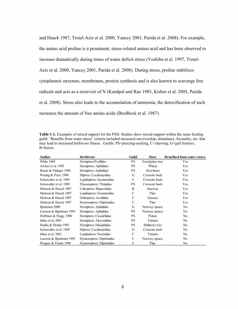
Table 1-1. Examples of mixed support for the PSH. Studies show mixed support within the same feeding guild. “Benefits from water stress” criteria included increased survivorship, abundance, fecundity, etc. that may lead to increased herbivore fitness. Guilds: PS=piercing-sucking, C=chewing, G=gall formers, B=borers

Author Herbivore Guild Host Benefited from water stress

White 1969 Hemiptera:Psyllidae PS Eucalyptus tree YesArcher et al. 1995 Hemiptera: Aphididae PS Wheat YesBraun & Flukiger 1984 Hemiptera: Aphididae PS Hawthorn YesWaring & Price 1990 Diptera: Cecidomyiidae G Creosote bush YesSchowalter et al. 1999 Lepidoptera: Geometridae C Creosote bush YesSchowalter et al. 1999 Thysanoptera: Thripidae PS Creosote bush YesMattson & Haack 1987 Coleoptera: Buprestidae B Quercus YesMattson & Haack 1987 Lepidoptera: Geometridae C Pine YesMattson & Haack 1987 Orthoptera: Acrididae C Grasses YesMattson & Haack 1987 Hymenoptera: Diprionidae C Pine YesBjorkman 2000 Hemiptera: Aphididae G Norway spruce NoLarsson & Bjorkman 1993 Hemiptera: Aphididae PS Norway spruce NoHoffman & Hogg. 1990 Hemiptera: Cicadellidae PS Potato NoInbar et al. 2001 Hemiptera: Aleyrodidae PS Tomato NoHanks & Denno 1993 Hemiptera: Diaspididae PS Mulberry tree NoSchowalter et al. 1999 Diptera: Cecidomyiidae G Creosote bush NoInbar et al. 2001 Lepidoptera: Noctuidae C Tomato NoLarsson & Bjorkman 1993 Hymenoptera: Diprionidae C Norway spruce NoWagner & Frantz 1990 Hymenoptera: Diprionidae C Pine No

9

Aside from repair, these spare photoassimilates also form the ROS scavenging

compounds mentioned above, providing aid through both osmosis and active ROS

removal. Consequently, the rise in carbohydrates and amino acids has been shown to

alter herbivore abundances due to changes in host nutritional quality (White 1969, 1984,

Huberty and Denno 2004, Scheirs and Bruyn 2005, Mody et al. 2009). This increase in

nutrients forms the basis for the “plant stress hypothesis” and has had mixed support

from numerous studies (Table 1-1) since it was originally proposed by White in 1969.

1.4 Water-deficit stress and herbivory

In 1969, T.C.R. White correlated water stress with outbreaks of psyllids

(Hemiptera: Psyllidae) on eucalyptus trees in Australia using a “stress index” based upon

seasonal rainfall. Trees were determined to be under stress when the amount of summer

rainfall was lower than that of the preceding winter’s rainfall. His study found that

positive stress indices, in which trees were experiencing water deficit stress, were

correlated with psyllid outbreaks across several decades throughout Australia. The

correlation was so strong that populations of psyllids were practically non-existent

during non-stress periods. He later postulated that the cause of this was increasing N

content in the trees due to stress induced osmolytes. As discussed earlier these

compounds contain N and aid in plant rehydration. White surmised that the basis of

psyllid outbreaks was based on increased N and therefore greater host nutritional quality

of eucalyptus, allowing the psyllids to thrive on hosts that are usually poor in nutritional

quality. With this observation, White formulated what is the “plant stress hypothesis”

10

(PSH), which states that herbivores may outbreak on water stressed plants due to

changes in plant physiology, mainly increases in foliar N (White 1969, 1984, Mattson

and Haack 1987, Waring and Price 1990, Huberty and Denno 2004). Since its

formulation, numerous studies have tested the PSH, finding mixed support (Table 1-1).

For example, Waring and Price (1990) observed that gall midges (Diptera:

Cecidomyiidae) had higher abundances on water stressed creosote bush (Larrea

tridenrutu) compared to non-stressed bushes. Schowalter et al. (1999) found several

defoliating lepidopteran species (Semiothesia) and thysanopteran (Frankliniella) species

that preferred creosote bushes under reduced water treatments. Archer et al. (1995)

demonstrated that aphids preferred stressed wheat versus fully irrigated wheat. Despite

this support, there is also just as much opposition. Schowalter et al. (1999) found gall

midges that did not prefer stressed creosote; in fact they highly preferred irrigated

bushes, the same bush species these gall midges preferred under stress (Waring and

Price 1990). In addition, leaf miners and chewers as well as whiteflies did not perform

well on stressed tomato plants and exhibited a preference for more vigorous plants (Inbar

et al. 2001). Empirical studies show mixed support for even the same feeding guild and

herbivore families (Table 1-1.) With such high variation in herbivore response to

stressed plants, attention needed to be directed to the studies themselves.

1.5 Huberty and Denno meta-analysis

There has been great difficulty in supporting the plant stress hypothesis, yet

White’s observations were sound in 1969. Support from empirical studies and

11

observations since the formulation of the PSH have been conflicted, with empirical

studies unable to support PSH. This begged the question as to what were the differences

between empirical studies and observations made in nature. This question and the

discrepancies in the literature were addressed more thoroughly by Huberty & Denno in

2004 (HD). They compiled 82 published studies relating to water deficit stress and

herbivore response, and discussed relative aspects of plant physiology and insect

ecology. HD compared leaf water and N content between stressed and non-stressed

plants, assessed the effects of stressed plants on the major feeding guilds (including PS

and chewing), and compared herbivore performance on stressed plants.

Overall, HD found that experimental studies did not support the plant stress

hypothesis for both PS and chewing herbivores. Density, fecundity, survivorship,

oviposition, and growth rate were either negatively affected or responded neutrally to the

effects of water stress. Despite increases in foliar N content, both PS and chewing

herbivores responded negatively to water stress. For example, chewing herbivores

exhibited a statistically neutral response caused by a declining response from free-living

chewers and gall formers and an increase in response by stem borers. PS herbivores

actually exhibited a greater negative response to water stress compared to chewing

herbivores and when comparing sub-guilds (mesophyll and phloem vs. stem borers,

gallers, miners, and free-living).

Our knowledge of the negative effects of water stress may help us formulate an

understanding of these results. For instance, the accumulation of allelochemicals and

decreases in plant turgor may undermine the benefits of increased N content by deterring

12

herbivores and reducing feeding efficiency. Inbar et al. (2001), observed an increase in

peroxidase and chitinases in water stressed plants (supported by Lorio Jr (1986)). Paré

and Tumlinson (1999) also stated that water stressed plants produced more volatiles than

non-stressed plants. We also know that a reduction in plant turgor pressure may result in

reduced feeding efficiency. Kennedy et al. (1958) supported that low turgor pressure

may lead to a decrease in aphid populations and even suggested that the return of turgor

after a drought may lead to outbreaks of aphids. The reduction in leaf area due to stress

may also result in significantly higher densities of trichomes, reducing herbivore feeding

preference (Gershenzon 1984). Leaf toughness and increases in defensive peroxidase

activity (insect malnutrition) are believed to be responsible (Inbar et al. 2001, Ruuhola

and Yang 2005). Tougher leaf foliage lowers the availability of foliar N through

mechanical defense and may result in decreased performance (McMillin and Wagner

1996). Stress induces a reduction in growth, allowing plants to produce more structural

defenses such as lignin instead of more cells, increasing plant toughness. Despite these

negative effects, osmolytes provide greater nutrition for herbivores and there are studies

such as White’s observations and the handful of experimental studies that do support the

PSH. So then what are the differences between the observational studies that support the

PSH and the experimental studies that do not? With plant physiology and literature

supporting the possibility that herbivores may both benefit or be impaired by stressed

plants, HD carefully examined the experimental designs of the 82 published studies to

piece the puzzle together. Eventually they identified several empirical issues that may

have led to high variation in herbivore response: 1) researchers did not independently

13

establish that the experimental plants were indeed water stressed (i.e. measurements of

photosynthetic rate, turgor, etc.). Therefore, whether the plant was indeed stressed and

the possible severity of that stress was not independently determined, allowing for the

possibility of discounted variation within “water stress” treatments. Researchers based

consequential physiological responses (i.e. fewer seeds, stunted growth) as a

measurement of water stress whereas these results may have been due to growing

conditions, variation within plant species, or other stresses, leaving room for

confounding effects on herbivores. 2) Water stress was not isolated from other forms of

stress such as water logging, pollution, excess light, etc., leading to a possible

compounding of all sorts of stress effects that affected herbivore response. The third and

most important note was that experimental drought situations were usually in the form of

continuous stress without any form of recovery, while intermittent or pulsed stress

occurs in nature. HD discussed that turgor pressure is key to understanding negative

responses from PS herbivores. Turgor is required for efficient PS feeding and they

rationalized that if water content dropped below a certain level, feeding efficiency is

dramatically reduced. They proposed a threshold level of leaf water content above which

feeding is efficient and if below leads to a decline in herbivore performance. For

example, Myzus persicae and Brevicoryne brassicae aphids exhibited lower feeding

efficiency when feeding on low turgor plants (Wearing 1972). White’s initial

documentation of the effects of water stress was in nature, where pulsed stress occurs.

Pulsed stress allows for the recovery of foliar water content and turgor pressure, which

has been shown to benefit both chewing and PS herbivores (Scriber 1977). HD deduced

14

that natural water stress scenarios have a periodic return of plant turgor and it is this in

combination with increased soluble N levels that lead to herbivore outbreaks, in

comparison to most experimental scenarios that do not raise turgor. Thus, the predictive

power of PSH depended heavily upon the type of stress, its duration, and its timing.

They therefore proposed the “Pulsed Stress Hypothesis” (PLSH) which hypothesized

that herbivores will respond positively to pulsed stress plants since these plants have the

turgor pressure necessary for herbivores to access stress-induced increases in nutrients.

1.6 After Huberty and Denno

Since HD’s meta-analysis, there have been various studies addressing the effects

of water stress on herbivore response. However, studies still report conflicting results for

PSH and even the PLSH, despite HDs noted experimental concerns. An Nguyen et al.

(2007) conducted a 14 day continuous stress study that showed that aphids did not

perform well on continuously stressed plants. Plants were only watered at the beginning

of the study and not once for 14 days, allowing “severe stress” to occur. An Nguyen’s

only measurement of stress was the observed stress at the end of the 14 day aphid assay.

Additionally, an observational sampling study was conducted by Trotter et al. (2008),

using forest systems with and without a historical record of varying degrees of drought

stress. They found that larger arthropod communities of herbivores, predators, and

parasitoids subsisted on low stress plants. This study conducted sampling in a 6-10 day

period during phenological maturation of pinyon-juniper woodlands in Arizona. Once

again issues can be brought to light, specifically that this study only provided a snapshot

15

of the community composition and current drought conditions. Prior water stress

conditions, including the type of stress, needed to be addressed in order to accurately

determine the significance of the conditions for the arthropod community. Furthermore,

a continuous stress experiment was conducted on Brassicaceae plants by Khan et al.

(2010), resulting in a positive response from a generalist aphid species (M. persicae) and

a neutral response from its specialist counterpart (B. brassicae). Once again this study

did not incorporate an independent measurement of water stress, allowing for similar

methodological concerns as noted above.

Mody et al. (2009) conducted a pulsed stress study involving apple plants,

Spodoptera littoralis caterpillars (Lepidoptera: Noctuidae), and Aphis pomi aphids. This

study utilized several physiological measurements that measured stress, including

stomatal conductance as a direct measurement. They also measured shoot and root

growth and N content in leaves. Unfortunately, the pulsed treatment was implemented

based on visible symptoms of stress, once again allowing for concerns as to the certainty

of stress severity. The low stress plants were watered when “wilting” and high stress

plants before visible necrosis. These methods raise concerns in that plants are stressed

and begin to accumulate osmolytes before they are wilting and further so before necrosis

(Lombardini 2006). The other issue in this study was the brevity of the “pulsed stress”.

Water was provided to the plants several hours before the addition of caterpillars, in

which the researchers stated provided adequate time for turgor recovery, however turgor

was not measured. The presence of pulsed stress is thereby questionable. This study,

however, was close to addressing the effects of pulsed stress on plant-insect interactions

16

since the HD review in 2004. Interestingly enough, this study supported the preference

of chewing herbivores on highly stressed plants and a negative response from aphids, a

contradiction to the pulsed stress hypothesis. Paine and Hanlon (2010) demonstrated that

psyllids respond neutrally to water stress even though they utilized a “pulsed” water

stress treatment. This study exhibited several flaws that HD specifically addressed as in

the study did not have a plant-specific measurement of stress and relied solely on soil

moisture fluctuations to indicate pulse stress. The lack of an independent measurement

of stress suggests that the researchers did not know how stressed the plants were, if the

supposed stress was significantly different between trees, and if the given soil moisture

was a direct correlate to water stress and plant water usage. These issues may have led to

a neutral response from psyllids.

The literature past and present indicates the need to address the effects of water

stress in a concise manner, employing a clear method of measuring water stress and

distinctly separating the differences between the effects of pulsed and continuous stress.

As I have mentioned, water stress dramatically changes the physiology of host plants

with each type of stress altering physiology in a different manner. As supported through

observational studies, herbivores may outbreak on water stressed plants; however,

currently we are unable to conclusively predict the effects of water stress on insect

herbivores. The HD analysis of herbivore response literature has revealed that pulsed

water stress may have been responsible for observed herbivore outbreaks, yet empirical

studies have yet to support this hypothesis fully.

17

1.7 Dissertation questions

For my dissertation, I will provide the evidence for PLSH’s ability or inability to

predict herbivore outbreaks with my main question: Can the pulsed stress hypothesis be

used to predict herbivore response to water stressed host plants? This question will be

critical to understanding the establishment and population dynamics of herbivores by

using the literature’s current water stress hypotheses. This question is important because

not only will it narrow the knowledge gap in herbivore response literature, but it will

also lead to understanding the occurrence of herbivore pest outbreaks in agriculture and

natural systems.

18

CHAPTER II

CONTINUOUS AND PULSED DROUGHT: THE EFFECTS OF VARYING WATER

STRESS ON COTTON PHYSIOLOGY

2.1 Introduction

Drought stress is predicted to become more prevalent with climate change and

have a greater impact on plant-insect interactions (Mishra and Singh 2010, Dai 2011,

Kiem and Austin 2013, Van Lanen et al. 2013). There has been an established interest in

predicting the effects of water stress on plant-insect interactions, with over 500

published studies (search results from Web of Knowledge, Google Scholar 2013) and

half a dozen formal hypotheses addressing the topic (White 1969, Price 1991, Huberty

and Denno 2004). Despite this intensive effort researchers still have difficulty accurately

predicting the effects of water stress on insect abundance. Variation in herbivore

response to water-stressed plants, for instance, has been attributed to differences in

herbivore feeding physiology, taxonomy, and natural history (Waring and Price 1990,

Herms and Mattson 1992, Hanks and Denno 1993, Larsson and Bjorkman 1993, Huberty

and Denno 2004, Mody et al. 2009, Gutbrodt et al. 2011). Aside from herbivores,

however, little attention has been given to determining the variation in stress-induced

changes in host plants and how this variation may contribute to differences in herbivore

response to water-stressed plants.

During water deficit stress plants accumulate primary metabolites

(macronutrients), digestible carbohydrates, antioxidant enzymes, and micronutrients to

19

alleviate stress (Hsiao 1973, Chaves et al. 2002, Jithesh et al. 2006, Ghannoum 2008,

Taiz and Zeiger 2010). For instance, the amino acid proline alleviates water stress by

stabilizing cell membranes, cytoplasmic enzymes, and scavenging free radicals (Jithesh

et al. 2006, Parida et al. 2008, Taiz and Zeiger 2010). The accumulation of these stress-

related compounds can also be beneficial to herbivores because they contain nitrogen

and essential nutrients for growth and development. On the other hand, water stress can

lead to tougher leaves, more trichomes, thicker surface waxes, and higher concentrations

of allelochemicals that negatively affect herbivores (Raupp 1985, Herms and Mattson

1992, Stamp 2003).

The extent to which water-stressed plants accumulate stress-related compounds

and negatively affect herbivores may be dependent upon the evolutionary history of the

plant and stress severity (Lorio Jr 1986, Ryser and Lambers 1995, Fine et al. 2004). For

example, the “Growth-Differentiation Balance Hypothesis” predicts that plants growing

in resource-poor conditions (e.g., water deficit limiting carbon uptake) will allocate

resources (e.g., chlorophyll, nitrogen, allelochemicals) to maintain and protect leaf tissue

to minimize investment in tissue regrowth due to herbivory (Coley et al. 1985, Lorio Jr

1986, Herms and Mattson 1992). The degree to which plants protect existing leaf tissue

and invest in potential regrowth, results in differences in photosynthesis and plant

biomass (Nash and Graves 1993, Durhman et al. 2006, Taiz and Zeiger 2010).

Additionally, the induction and magnitude of these stress-related changes in plants

fluctuate with continued and increased severity of water stress (Hsiao 1973, Coley et al.

1985, Chaves et al. 2002, Chaves et al. 2003). For instance, long periods of drought, or

20

continuous water stress, result in a decline in photosynthesis, stomatal conductance,

water potential, and increases in stress-related compounds compared to mildly stressed

plants (Baskin and Baskin 1974, Tezara et al. 1999, Huberty and Denno 2004, Parida et

al. 2008, Lawlor and Tezara 2009, Taiz and Zeiger 2010). In contrast, the “Pulsed Stress

Hypothesis” (intermittent water stress) suggests that when plants recover from stress,

plants may reduce the deleterious effects of water stress and improve plant quality for

herbivores. Previous studies, however, tend to generalize the effects of water stress on

host plants, often overlooking the effects of stress severity and duration on host plants.

Incorporating the contrasting effects of pulsed and continuous stress into a single basis to

predict herbivore performance may have resulted in the variation in studies testing

herbivore response to water-stressed plants. To our knowledge, studies have not directly

compared the effects of pulsed and continuous stress simultaneously under the same

experimental conditions. Understanding the differences in how stress severity and

duration affect stressed host plants may help us more accurately predict herbivore

response to water-stressed plants.

In our study, we measured stress-related changes in cotton plants in response to

pulsed and continuous water stress in an agro-ecosystem. Our goal was to determine

how different types of water stress influence cotton physiology and may lead to

differences in host plant quality for herbivores. We measured photosynthesis, stomatal

conductance, transpiration efficiency, relative chlorophyll content, nutrients, antioxidant

enzymes, stem water potential, soil moisture, and plant development. We hypothesized

that pulsed stressed plants will have increased nutrients, water potential, and

21

photosynthesis to predictably increase host plant quality compared to continuously

stressed plants. Continuously stressed plants, however, will have greater chlorophyll

content and be less developed in conjunction with the growth-differentiation balance

hypothesis. Differences in photosynthesis, nutrients, and plant development between

pulsed and continuously stressed plants should produce differences in plant quality for

insect herbivores and affect herbivores differently.

2.2 Methods

2.2.1 Study system

We conducted two, 10-week field studies in 2010 and 2011 at the Texas A&M

Field Laboratory in Burleson County, Texas (coordinates: 30.548754,-96.436082). The

south-central region of Texas experiences subtropical and temperate climates with mild

winters lasting no longer than two months. High temperatures range from 25°C in May

to 35°C in July, and precipitation ranges from 11.94cm in May to 5.08cm in July. Our

field site primarily consisted of Belk series clay soil, known as a very deep, well drained,

and slowly permeable soil that is common in Texas flood plains (U.S.A. 2007).

Approximately 0.6 hectares of cotton were planted in both 2010 and 2011. We planted

commercial cotton (Gossypium hirsutum L.), Delta Pine 174RF (no drought/pest

resistance), on 3 May 2010. Cotton was furrow irrigated on 14 May and treatments

began on 14 June when cotton reached the late seedling, early squaring (flower bud)

stage. In 2011, the same cotton variety was planted on 18 April and irrigated on 21 May

before treatments began on 13 June during the late seedling-early squaring stage. The

22

study concluded on 29 and 28 August in 2010 and 2011, respectively. The field was

treated with Round-Up herbicide to eliminate weeds and fertilized with 14.69 kg of

nitrogen/hectare with a time-release formula for both years.

2.2.2 Experimental design

Cotton was divided into 54, 6 m x 4.5 m plots, separated into 9 blocks and each

block randomly received continuous stress, pulsed stress, or control irrigation treatments.

Each treatment had 6 plots per block for a total of 18 plots per treatment in a randomized

complete block design. Blocks had 9.1 m of untreated cotton on all sides and each plot

within a block had 2.7 m of untreated cotton between plots. Continuously water stressed

plants were not irrigated for the entire growing season and only received ambient

rainfall, while the control plants received irrigation weekly. For the pulsed stressed

plants, we used a pressure chamber (model 615, PMS Instrument Co., Albany, OR) to

measure water status and determine the appropriate stress level to trigger irrigation.

Cotton plants are water-stressed at approximately -1.2 MPa (-12 bars) and begin to

accumulate stress-induced increases in foliar nitrogen and other nutrients (Hsiao 1973,

Lombardini 2006). Pulsed stressed plants were watered when their stem water potential

was below -1.2 MPa. For the pressure chamber measurements, 17 cm x 9 cm aluminum

bags were placed over the uppermost, fully-expanded leaf for 20 minutes, and then

clipped at the proximal end of the petiole using scissors. The aluminum bag, with the

leaf still inside, was then folded gently and inserted into the chamber for a pressure

reading. To accommodate for destructive sampling for pressure chamber measurements,

23

each plot was divided into 32 subplots containing 10-15 plants and one plot was

randomly selected for pressure chamber measurements each week, for a total of 18

measurements each week per treatment. This subplot method was used for all

measurements to avoid sampling the same plants.

2.2.3 Soil moisture, photosynthesis, stomatal conductance, and transpiration efficiency

Soil moisture data was collected using a soil corer to remove a 212 cm3 soil

sample in every 1st, 4th, and 6th plot of each block, between plants outside of furrows.

The soil sample was weighed for wet weight, dried at 60°C for two days in a Thermo

Precision drying oven (model 6524, Thermo Fisher Scientific, Inc., Waltham, MA), and

the dry weight recorded.

Photosynthetic rate, stomatal conductance of water, and transpiration efficiency

were measured using a LI-COR portable photosynthesis system model LI-64000XT (LI-

COR, Inc., Lincoln, Nebraska). Transpiration efficiency (TE) was calculated from the

LI-COR photosynthetic rate and transpiration data with: TE= photosynthetic rate (µmol

CO2/m2s)/transpiration rate (mmol H2O/ m2s) similarly to Hubick et al. (1988) and

Masle et al. (2005). LI-COR measurements were taken during optimal daylight hours

from 9am to 2pm on the uppermost, fully expanded leaf with three measurements per

leaf for each plot measured. To complete the measurements for all 9 blocks between 9am

and 2pm, the 1st, 4th, and 6th plot of each block was measured per treatment for a total of

9 measurements per treatment per week.

24

2.2.4 Chlorophyll fluorescence, relative chlorophyll content, and peroxidase assay

Chlorophyll fluorescence was measured using a chlorophyll fluorometer (model

OS30p, Opti-Sciences Inc., Hudson, NH) on the uppermost, fully expanded leaf. Prior to

each measurement, a single 1.5 cm diameter, light-excluding clip was placed over the

upper leaf surface for 20 minutes to render the surface dark-adapted. The fluorometer

was then inserted into the clip and the measurement was taken. Fluorescence data was

recorded as the maximum quantum efficiency: Fv/Fm= ((FMaximum fluorescence - FO(minimum

fluorescence) )/Fmaximum fluorescence).

Relative chlorophyll content was measured using a chlorophyll meter (SPAD

model 502, Konica Minolta Sensing, Inc., Tokyo, Japan) on the uppermost, fully

expanded leaf of 5 plants per plot per block each week of the season. The SPAD-502

provides non-destructive measurements of relative chlorophyll content and has been

used to monitor the nitrogen nutritional status of maize, rice, potato, and cotton (Vos and

Bom 1993, Feibo et al. 1998, Chang and Robison 2003).

Peroxidase is an antioxidant enzyme in plants that neutralizes reactive oxygen

species that destroy photosystems in chloroplasts during water stress and has been

shown to become more concentrated in plants during water stress (Chaves et al. 2002,

Jithesh et al. 2006, Taiz and Zeiger 2010). Each week, the uppermost fully-expanded

leaf of 5 plants within a randomly selected subplot was removed. Leaves were quickly

and gently placed into 9 cm x 5.75 cm coin envelopes, stored in ice coolers, and quickly

transported to the laboratory. The envelopes were placed in -80°C freezers until assayed.

Proteins for the peroxidase assay were extracted using 275 mg of plant tissue ground in

25

15 µl of 0.01M sodium phosphate buffer at pH 6.8. Once ground, samples were

centrifuged at 12,000 rpm for 12 minutes, and the supernatant was kept and stored at -

20°C until assayed. For the assay, 2 µl of extracted proteins were added to a 96-well

plate in duplicate and 150 µl of 0.01M guaiacol solution at pH 6.0 was added to each

well. Samples and plates were kept on ice. The plates containing extracted proteins and

guaiacol solution were read by a microplate reader (model 680, Bio-Rad Laboratories

Inc., Hercules, CA) at 470 nm. Peroxidase activity was quantified by the following

equation: POD activity = (absorbance reading from software/1000)/(sample mass*0.015)

and expressed as ΔAbs470/min/gFW.

2.2.5 Amino acid and digestible carbohydrate assays

The leaves used for the peroxidase assay were also used for the amino acid and

digestible carbohydrate assays. Plant chemistry assays for amino acids were conducted

using a modified ninhydrin assay as according to Starcher (2001) and McArthur et al.

(2010). Ten samples were randomly chosen per treatment from each week of the study to

measure changes in amino acid concentration over time. For each sample, approximately

5 mg of tissue were removed and ground in 10 µl of 80% ethanol in an Eppendorf tube

using a manual tissue grinder and placed on ice. Once the tissue was ground, 500 µl of

6N HCl was added to the sample tube and placed in a heating block at 100°C for 24

hours. A large block was placed on top of the tubes to ensure that the caps stayed closed.

During the last 2.5 hours of the 24 hour period, the large blocks were removed and each

tube was opened to allow the HCl to boil off. The remaining pellet was suspended in 1

26

ml of water and centrifuged at 12,000 rpm for 1 minute to facilitate sample

homogeneity. The ninhydrin stock solution was prepared using 200 mg of ninhydrin, 7.5

ml of ethylene glycol, 2.5 ml of 4N sodium acetate buffer and 200 µl of stannous

chloride solution. In a new Eppendorf tube, 20 µl of sample and 100 µl of the ninhydrin

solution were added and returned to the 100°C heating block for 10 minutes. Samples

were cooled at room temperature and the sample and ninhydrin mixtures were

transferred to a 96-well plate. Plates were read at 570 nm using an Epoch microplate

reader (BioTek Instruments Inc., Winooski, VT). If samples were too dark to be read at

570 nm due to high amino acid content, 620 nm was used and a simple linear regression

equation was generated to convert amino acid concentrations from readings at 620 nm to

predicted concentrations at 570 nm. Amino acid standards were prepared using

powdered BSA (Sigma-Aldrich, St. Louis, MO) with dilutions prepared at 2 µg, 4 µg, 6

µg, 8 µg, and 10 µg/1 ml of water from 10 mg/1 ml of water. Standards were used to

generate a standard curve to approximate µg of amino acids/5 mg of plant tissue sample.

Plant chemistry assays for digestible carbohydrate content were conducted using

a phenol-sulfuric acid assay as according to Smith et al. (1964) and Clissold et al.

(2006). Ten frozen samples were randomly selected per treatment from each week of the

study to measure changes in digestible carbohydrates over time. Approximately 200 mg

of leaf tissue from each sample was freeze-dried (model UX-03336-73, Labconco,

Kansas City, MO) at -50°C for two days. Once dried, samples were ground to powdered

flakes using a MF 10 basic wiley cutting mill (IKA Works, Inc., Wilmington, NC) using

a size 20 mesh and 20 mg were removed and added to screw-cap test tubes. Each tube

27

received 1 ml of 0.1M sulfuric acid and was placed in a boiling water bath for 1 hour.

Tubes were cooled in a container of room temperature water, emptied into 1.5 ml

Eppendorf tubes, and mixed in a centrifuge at 13,000 rpm for 10 minutes. Each tube had

15 µl of supernatant removed which was added to glass test tubes with 385 µl of distilled

water and 400 µl of 5% phenol solution. Tubes then received 2 ml of concentrated

sulfuric acid and allowed to sit for 10 minutes. Samples were mixed for several seconds

using a vortex mixer then allowed to sit for an additional 30 minutes. Carbohydrate

standards were prepared using 0.2 mg/µl glucose to make six 400 µl dilutions containing

0, 15, 30, 45, 60, or 75 µg of glucose. The dilutions were treated in the same manner as

the samples with the same concentrations of phenol and sulfuric acid added in the same

manner. After sitting, 750µl of the sample, phenol, and sulfuric acid mixture was added

to cuvettes for spectrophotometric measurements at 490 nm with the samples being

measured in duplicates and the standards in triplicate. The standards were used to

generate a standard curve to approximate µg of digestible carbohydrates/20 mg of dried

plant tissue.

2.2.6 Cotton development

Plant height and nodes were counted in all plots during weeks 3, 6, and 9 during

the 2010 season and during weeks 1, 4, 6, and 9 during the 2011 season. In addition, the

quantity of squares and bolls were recorded for the first fruiting position (most

economically important bolls) in 2010 and for the entire plant in 2011.

28

2.2.7 Analysis

All measurements conducted in the study were analyzed using univariate

repeated measures ANOVA with JMP 10.0.0 (SAS Institute, Cary, NC) to make

comparisons between treatments over time. Sphericity tests were conducted for all

repeated measures to ensure that the variance assumptions of repeated measures were

not violated and analyses were accurate. If sphericity was violated and a corrective

Greenhouse-Geisser test yielded an Ɛ of > 0.75, then the corrected test was used. If the

Greenhouse-Geisser test yielded an Ɛ of < 0.75, then a MANOVA was used to generate a

Wilk’s lambda test statistic (Λ) to compare treatments over time. These adjustments

ensured that the most appropriate and powerful test was used to analyze the data.

Weekly and season average data were analyzed for relative SPAD values, amino acids,

digestible carbohydrates, photosynthetic rate, stomatal conductance, transpiration

efficiency, and peroxidase activity. Weekly data was analyzed for stem water potential,

soil moisture, chlorophyll fluorescence, and cotton development. In addition, for those

measurements with season average data, data was also reported for the weeks in which

pulse stressed plants were watered, during which the pulse stressed hypothesis can make

predictions of herbivore abundance. There were several weeks in the data during the

season in which the season average and pulses were not reported due to unforeseen

circumstances encountered in the field. LI-COR data (photosynthetic rate, stomatal

conductance, transpiration efficiency) and chlorophyll fluorescence were reported for the

2010 season. Data on season average and pulse concentrations of amino acids and

digestible carbohydrates were analyzed relative to the control (control= 0).

29

2.3 Results

2.3.1 Stem water potential and soil moisture

Water stress had strong effects on stem water potential. In 2010, stem water

potential varied throughout the season (stem water potential: F23, 408= 78.39, p<0.0001),

with treatment (treatment: F2, 429= 246.33, p<0.0001), and with treatment over time

(treatment*week: F14, 417= 24.24, p<0.0001) (Fig. 2-1A). In addition, control plants

maintained stem water potential above -1.2 MPa throughout the season, while

continuously stressed plants decreased stem water potential -1.2 MPa during week 5 and

decreased to -2.5 as the season concluded (Fig. 2-1A). Stem water potential in pulsed

stressed plants decreased below -1.2 MPa by week 5 and received irrigation at the end of

weeks 5 and 6 (black circles around weeks on x-axis; Fig. 2-1A). Pulsed stressed plants

were watered during week 5 and 9 to produce one pulse during week 6 (Fig. 2-1A).

In 2011, stem water potential varied throughout the season (stem water potential:

F10.5, 267.8= 28.87, p<0.0001), with treatment (treatment: F2, 465= 258.18, p<0.0001), and

with treatment over time (treatment*week: F10.5, 267.8= 28.87, p<0.0001) (Fig. 2-1B).

Control plants stem water potential below -1.2 MPa during weeks 8 and 9. Continuously

stressed plants decreased stem water potential below -1.2 MPa by week 4 and to -3 MPa

as the season concluded (Fig. 2-1B). Pulsed stressed plants decreased pressure below -

1.2 MPa by week 4 in 2011 and received irrigation at the end of weeks 4, 7, and 9 (black

circles around weeks on the x-axis; Fig. 2-1B). Furthermore, pulsed stressed plants were

water-stressed during weeks 4, 7, 8, and 9 and were watered thereafter to give them

pulses during weeks 5, 8, and 10 (Fig. 2-1B).

30

Figure 2-1. Stem water potential for stressed plants in 2010 and 2011. 2010 (A) and 2011 (B). The markers are mean stem water potential +SE. The dotted line marks -1.2 MPa, when plants are believed to be water-stressed. Circles over certain weeks indicate when the pulsed stress treatment received irrigation to end water stress. The “pulses” were during week 6 in 2010, and during weeks 5, 8, and 10 in 2011. Asterisks indicate significant differences between at least two of the three treatments for a given week.

Soil moisture was reflective of watering treatments during both years. In 2010,

soil moisture varied throughout the season (soil moisture: Λ= 0.17, F8, 42= 7.65,

p<0.0001), with treatment (treatment: F2, 132= 106.81, p<0.0001) and with treatment over

time (treatment*week: Λ= 0.17, F8, 42= 7.65, p<0.0001) (Fig. 2-2A). Furthermore, during

the pulse, pulsed stressed plants increased in soil moisture and remained greater than that

of continuously stressed plants until week nine, while continuously stressed plants

remained at approximately 4-6.5% throughout the season (Fig. 2-2A). In 2011, soil

A)

B)

31

moisture varied throughout the season (soil moisture: Λ= 0.02, F16, 34= 12.68, p<0.0001),

with treatment (treatment: F2, 240= 104.48, p<0.0001), and with treatment over time

(treatment*week: Λ= 0.02, F16, 34= 12.68, p<0.0001). During the pulses in week five and

eight, pulsed stressed plants had higher soil moisture than continuously stressed plants

and matched the soil moisture of control treated plants. Continuously stressed plants

declined in soil moisture from 20% during week 1 to 10% by week 9 (Fig. 2-2B).

Figure 2-2. Soil moisture % during field studies in 2010 and 2011. 2010 (A) and 2011 (B). The markers are mean soil moisture % +SE. Circles over certain weeks indicate when the pulsed stress treatment received irrigation to end water stress. The “pulses” were during week 6 in 2010, and during weeks 5, 8, and 10 in 2011. Asterisks indicate significant differences between at least two of the three treatments for a given week.

32

2.3.2 Photosynthesis, stomatal conductance, and transpiration efficiency

The pulse in 2010 had minimal effect on weekly photosynthetic rate in pulsed

stressed plants, but there were strong contrasts between treatments for the weekly

measurements and the season average. Photosynthetic rate varied during the season

(photosynthetic rate: F20, 168= 5.94, p<0.0001), with treatment (treatment: F2, 186= 11.07,

p<0.0001) and with treatment over time (treatment*week: F12, 176= 5.24, p<0.0001) (Fig.

2-3A). In addition, the season average of photosynthetic rate varied among treatments

Figure 2-3. Photosynthetic rate for stressed plants in 2010. Photosynthetic rate for the season (A), the average for the season (B), and during the pulse during week 6 in 2010 (C). The markers are mean photosynthetic rate +SE. Asterisks indicate significant differences between at least two of the three treatments for a given week. Bars are mean photosynthetic rate +SE. Bars with different letters above them are significantly different.

33

(season average: F2, 186= 7.84, p= 0.0005; Fig. 2-3B), but treatment did not affect

photosynthetic rate during the pulse in week six (treatment: F2, 24= 0.65, p= 0.5332; Fig.

2-3C). Moreover, weekly photosynthetic rates were similar between stressed plants for

the majority of the season, then diverged during week 7 with continuously stressed

plants decreasing to a photosynthetic rate of 12µmol CO2/m2s compared to 22 µmol

CO2/m2s in pulsed stressed plants during week 9 (Fig. 2-3A). Additionally, pulsed

stressed plants had a 13% greater photosynthetic rate on average compared to

continuously stressed plants throughout the season and were not significantly different

than control plants (Fig. 2-3B).

Stomatal conductance of water did not vary during the pulse in 2010, but varied

between stress treatments. Stomatal conductance varied throughout the season (stomatal

conductance: F20, 167= 10.84, p<0.0001), was significantly affected by treatment

(treatment: F2, 185= 43.30, p<0.0001), and was affected by treatment over time

(treatment*week: F12, 175= 7.74, p<0.0001). Stomatal conductance was similar between

stressed treatments until week 7 in which continuously stressed plants decreased 62%

compared to the previous week, while pulse stressed plants decreased 11% (Fig. 2-4A).

Season average of stomatal conductance varied between treatments (season average: F2,

185= 027.19, p<0.0001) with pulsed stressed plants 30% higher on average compared to

continuously stressed plants (Fig. 2-4B).

34

Figure 2-4. Stomatal conductance in stressed plants in 2010. Stomatal conductance of water for the season (A), the average for the season (B), and during the pulse during week 6 in 2010 (C). The markers are mean stomatal conductance +SE. Asterisks indicate significant differences between at least two of the three treatments for a given week. Bars are mean stomatal conductance +SE. Bars with different letters above them are significantly different. Transpiration efficiency varied among treatments during the second half the

season. Overall, transpiration efficiency varied throughout the season (transpiration

efficiency: Λ= 0.3, F12, 38= 2.66, p= 0.0108), with treatment (treatment: F2, 187= 12.91,

p<0.0001), with treatment over time (treatment*week: Λ= 0.3, F12, 38= 2.66, p= 0.0108)

(Fig. 2-5A). During week 7, continuously stressed plants had a 13% higher transpiration

efficiency than pulsed stressed plants and remained similar in efficiency at week 9 (Fig.

2-5A). In addition, the season average for transpiration efficiency was significantly

35

affected by treatment (season average: F2, 187= 7.36, p= 0.0008; Fig. 2-5B), but was not

affected by treatments during the pulse (treatment: F2, 24= 1.43, p= 0.2592; Fig. 2-5C).

Furthermore, transpiration efficiency was 9% higher in continuously stressed plants

compared to pulsed stressed plants on average throughout the season (Fig. 2-5B).

Figure 2-5. Transpiration efficiency in stressed plants in 2010. Transpiration efficiency for the season (A), the average for the season (B), and during the pulse during week 6 in 2010 (C). Transpiration efficiency= photosynthetic rate (µmol CO2/m2s)/transpiration rate (mmol H2O/ m2s). The markers are transpiration efficiency+SE. Asterisks indicate significant differences between at least two of the three treatments for a given week. Bars are mean transpiration efficiency +SE. Bars with different letters above them are significantly different.

B) A)

C)

36

2.3.3 Chlorophyll fluorescence, relative chlorophyll content, and peroxidase assay

Chlorophyll fluorescence (maximum quantum efficiency) did not vary between

stress treatments. Fluorescence varied over the season (fluorescence: F20, 351= 5.65,

p<0.0001) and with treatment over time (treatment*week: F14, 383= 3.44, p<0.0001), but

treatment alone did not have an effect (treatment: F2, 395= 0.21, p= 0.8109) (Fig. 2-6).

Fluorescence was significantly different between stressed plants during week 9, in which

pulsed stressed plants had a 10% greater quantum efficiency compared to continuously

stressed plants.

Figure 2-6. Chlorophyll fluorescence in stressed plants in 2011. The markers are mean maximum quantum efficiency +SE. Asterisks indicate significant differences between at least two of the three treatments for a given week.

There were strong differences in relative chlorophyll content between stress

treatments in 2010. SPAD values varied throughout the season (chlorophyll content: F26,

435= 48.11, p<0.0001), with treatment (treatment: F2, 459= 327.47, p<0.0001), and with

treatment over time (treatment*week: F16, 445= 17.00, p<0.0001) (Fig. 2-7A).

37

Furthermore, continuously stressed plants contained significantly more chlorophyll

during most of the season with SPAD values ranging from 36 to 40 from week 6 to 9,

while pulsed stressed plants ranged from 30 to 34 (Fig. 2-7A). SPAD values varied on

average (season average: F2, 459= 160.05, p<0.0001; Fig. 2-7B) and during the pulse in

2010 (chlorophyll content: F2, 51= 51.82, p<0.0001; Fig. 2-7C). Continuously stressed

plants were 12% higher in SPAD values compared to pulsed stressed plants on average

throughout the season (Fig. 2-7B), and 20% higher during the pulse in 2010 (Fig. 2-7C).

Figure 2-7. Relative chlorophyll content (SPAD values) in 2010. The effects of water stress on relative chlorophyll content using a SPAD meter for the season (A), the average for the season (B), and during the pulse during week 6 in 2010 (C). The markers are mean SPAD values +SE. Asterisks indicate significant differences between at least two of the three treatments for a given week. Bars are mean SPAD values +SE. Bars with different letters above them are significantly different.

C)

A) B)

38

In 2011, differences in relative chlorophyll content between stress treatments

were not as pronounced. Overall, SPAD values varied throughout the season

(chlorophyll content: F20, 357= 20.77, p<0.0001), with treatment (treatment: F2, 375=

130.03, p<0.0001), and with treatment over time (treatment*week: F12, 365= 5.22,

p<0.0001) (Fig. 2-8A). Stressed plants were significantly greater in chlorophyll content

compared to control plants for the majority of the season (Fig. 2-8A). In addition,

Figure 2-8. Relative chlorophyll content (SPAD values) in 2011. The season (A), the average for the season (B), and during the pulse during the third pulse in week 10 in 2011 (C). The markers are mean SPAD values +SE. Asterisks indicate significant differences between at least two of the three treatments for a given week. Bars are mean SPAD values +SE. Bars with different letters above them are significantly different.

B) A)

C)

39

stressed plants were similar in SPAD values on average for the season (season average:

F2, 375= 95.16, p<0.0001; Fig. 2-8B) and during the pulse in week 10 (treatment: F2, 51=

28.07, p<0.0001; Fig. 2-8C), but were significantly greater in chlorophyll content

compared to control plants in both cases (Figs. 2-8B and 2-8C).

Peroxidase activity did not vary throughout the season (POD activity: Λ= 0.94,

F6, 96= 0.52, p= 0.7915), did not differ with treatment (treatment: F2, 274= 1.77, p=

0.1716), and did not vary with treatment over time (treatment*week: Λ= 0.94, F6, 96=

0.52, p= 0.7915) (Fig. 2-9A). Average peroxidase activity was not affected by treatment

Figure 2-9. Peroxidase activity in stressed plants in 2010. Activity for the season (A), season average (B), and the week 6 pulse in 2010 (C). The markers and bars are mean peroxidase activity +SE. Asterisks indicate significant differences. Bars with different letters above them are significantly different and letters with asterisks indicate a marginal significant difference.

B) A)

C)

40

(season average: F2, 274= 1.90, p= 0.1515; Fig. 2-9B), but was marginally different

between pulsed stressed and control plants (Fig. 2-9B). Additionally, peroxidase activity

was similar for the treatments during the pulse in 2010 (treatments: F2, 51= 0.99, p=

0.3777; Fig. 2-9C).

Peroxidase activity in 2011 did not vary throughout the season (POD activity: Λ=

0.6, F16, 62= 1.11, p= 0.3622), varied with treatment (treatment: F2, 441= 6.11, p= 0.0024),

and did not vary with treatment over time (POD activity: Λ= 0.6, F16, 62= 1.11, p=

0.3622) (Fig. 2-10). Activity was similar between treatments until a large peak during

week 8, but the stress treatments were similar (Fig. 2-10A). Furthermore, peroxidase

activity varied in the season average (season average: F2, 441= 4.13, p= 0.0167; Fig. 2-

10B), but pulsed and continuously stressed plants were similar (Fig. 2-10B). During the

pulse in week 5, peroxidase activity significantly varied with treatment (treatment: F2,

46= 4.30, p= 0.0194; Fig. 2-10C) while pulsed stressed plants were 500% lower in

activity compared to continuously stressed plants (Fig. 2-10C). During the second pulse

in week 8, peroxidase activity also varied by treatment (treatment: F2, 50= 5.42, p=

0.0074; Fig. 2-10D), but stressed plants were similar (Fig. 2-10D).

2.3.4 Amino acid and digestible carbohydrate assays

Concentrations of amino acids were similar in stressed plants during the season,

but there were a few notable contrasts. In 2010, concentrations of amino acids varied

throughout the season (amino acids: F20, 188= 17.66, p<0.0001), with treatment

41

(treatment: F2, 206= 16.77, p<0.0001), and with treatment over time (treatment*week: F2,

24= 2.33, p= 0.0084) (Fig. 2-11A). In addition, there was a significant difference

Figure 2-10. Peroxidase activity in stressed plants in 2011. Peroxidase activity for the season (A), the average for the season (B), during the pulse during week 5 in 2011(C), and the pulse during week 8 in 2011. The markers are mean peroxidase activity +SE. Asterisks indicate significant differences between at least two of the three treatments for a given week. Bars are mean peroxidase activity +SE. Bars with different letters above them are significantly different. between stressed plants for the season average (F1, 138= 10.87, p= 0.0012; Fig. 2-11B)

and pulsed stressed plants had a 250% lower concentration of amino acids (Fig. 2-11B).

During the pulse however, treatments had no effect on amino acids (treatment: F1, 18=

1.24, p= 0.2809; Fig. 2-11C).

B) A)

C) D)

42

Water stress did not affect concentrations of amino acids during most of the

season in 2011. Overall, amino acids varied throughout the season (amino acids: Λ=

0.28, F12, 42= 3.08, p= 0.0034), with treatments (treatment: F2, 265= 5.04, p= 0.0072), and

with treatment over time (treatment*week: Λ= 0.28, F12, 42= 3.08, p= 0.0034) (Fig. 2-

12A). In addition, the season average did not differ between stress treatments (treatment:

F1, 179= 1.03, p= 0.3113; Fig. 2-12B). During the pulse in week 5 in 2011, stressed plants

had similar concentrations amino acids (F1, 18=1.10, p= 0.3074; Fig. 2-12C), but were

marginally different during the second pulse (F1, 18= 4.28, p= 0.0532; Fig. 2-12D).

Figure 2-11. Amino acids in stressed plants in 2010. Concentrations of amino acids for the season (A), the average for the season relative to the control (B), and during the pulse during week 6 in 2010 relative to the control (C). The markers are mean amino acid concentrations +SE. Asterisks indicate significant differences between at least two of the three treatments for a given week. Bars are mean amino acid concentrations +SE. Bars with different letters above them are significantly different.

B) A)

C)

43

Figure 2-12. Amino acids in stressed plants in 2011. Concentrations of amino acids for the season (A), the average for the season relative to control plants (B), the pulse during week 5 in 2011 relative to control plants (C), and the pulse during week 8 in 2011 relative to control plants. The markers are mean concentrations of amino acids +SE. Asterisks indicate significant differences between at least two of the three treatments for a given week. Bars are mean concentrations of amino acids +SE. Bars with different letters above them are significantly different and letters with asterisks indicate a marginal significant difference.

Water stressed plants had similar concentrations of digestible carbohydrates in

2010. Carbohydrates did not vary throughout the season (carbohydrates: F6.1, 79.6= 1.28,

p= 0.2742), varied with treatment (treatment: F2, 146= 7.47, p= 0.0008), but did not vary

with treatment over time (treatment*week: F6.1, 79.6= 1.28, p= 0.2742) (Fig. 2-13A). For

the season average, carbohydrates were similar among stressed plants (season average:

F1, 98= 1.01, p= 0.3173; Fig. 2-13B), and treatments had a similar effect on

B) A)

C) D)

44

carbohydrates after the pulse during week 7 (treatment: F1, 18= 0.20, p= 0.6587; Fig. 2-

13C).

Figure 2-13. Digestible carbohydrates in stressed plants in 2010. Concentrations of digestible carbohydrates for the season (A), the average for the season relative to the control (B), and during the pulse during week 6 in 2010 relative to the control (C). The markers are mean digestible carbohydrates concentrations +SE. Asterisks indicate significant differences between at least two of the three treatments for a given week. Bars are mean digestible carbohydrates concentrations +SE. Bars with different letters above them are significantly different.

In 2011, carbohydrates in stressed plants were similar for the majority of the

season. Overall, carbohydrates varied throughout the season (carbohydrates: F14, 133=

2.35, p= 0.0060), with treatment (treatment: F2, 145= 1.38, p= 0.2545), and with treatment

over time (treatment*week: F8, 139= 1.68, p= 0.1087) (Fig. 2-14A). Additionally,

B) A)

C)

45

carbohydrates were similar in concentration on average throughout the season (season

average: F1, 97= 2.40, p= 0.1242; Fig. 2-14B) and stressed plants were similar during the

first pulse in week five (treatment: F1, 18= 0.07, p= 0.8002; Fig. 2-14C). Furthermore,

stress type had significantly different effects on carbohydrates during the second pulse in

week 8 (treatment: F1, 18= 27.56, p<0.0001; Fig. 2-14D) and continuously stressed plants

had seven times lower concentrations of carbohydrates compared to pulsed stressed

plants (Fig. 2-14D).

Figure 2-14. Digestible carbohydrates in stressed plants in 2011. Concentrations of digestible carbohydrates for the season (A), the average for the season relative to control plants (B), the pulse during week 5 in 2011 relative to control plants (C), and the pulse during week 8 in 2011 relative to control plants. The markers are mean digestible carbohydrates +SE. Asterisks indicate significant differences between at least two of the three treatments for a given week. Bars are mean concentrations of digestible carbohydrates +SE. Bars with different letters above them are significantly different.

B) A)

C) D)

46

2.3.5 Cotton development

Water stress significantly affected cotton height, nodes, and the quantity of

squares and bolls in 2010. Plant height significantly varied throughout the season

(height: F8, 152= 164.26, p<0.0001), by treatment (treatment: F2, 158= 102.19, p<0.0001),

and with treatment over time (treatment*week: F4, 156= 17.89, p<0.0001) (Fig. 2-15A).

For instance, pulsed stressed plants were significantly taller than continuously stressed

plants, with pulsed stressed plants 30% taller than continuously stressed plants at week

9. Furthermore, the number of nodes varied throughout the season (nodes: F8, 152= 60.39,

Figure 2-15. Plant height, total nodes, and total 1st position squares and bolls in 2010. Plant height (A), nodes (B), and first position squares and bolls in 2010 (C). The markers are means +SE. Asterisks indicate significant differences between at least two of the three treatments for a given week.

A) B)

C)

47

p<0.0001; Fig. 2-15B), with treatment (treatment: F2, 158= 52.03, p<0.0001), and with

treatment over time (treatment*week: F4, 156= 29.19, p<0.0001) (Fig. 2-15B). In

addition, there were significant differences in nodes between treatments during week 3,

similarities during week 6, and pulsed stressed plants had 60% more nodes than

continuously stressed plants by week 9 (Fig. 2-15B). For first position squares and bolls,

the total varied throughout the season (squares and bolls: F3.1, 77.3= 7.52, p= 0.0002),

with treatment (treatment: F2, 158= 10.55, p<0.0001), and with treatment over time

(treatment*week: F3.1, 77.3= 7.52, p= 0.0002). For example, pulsed stressed plants had

220% more first position squares and bolls by week 9 (Fig. 2-15C).

In 2011, water stressed significantly reduced plant height, quantity of nodes, and

total squares and bolls. Plant height varied throughout the season (height: F6, 153= 25.96,

p<0.0001), with treatment (treatment: F2, 213= 116.96, p<0.0001), and with treatment

over time (treatment*week: F6, 153= 25.96, p<0.0001) (Fig. 2-16A). For instance, pulsed

stressed plants were 20% taller than continuously stressed plants by week 9. For quantity

of nodes, quantity varied throughout the season (nodes: F11, 204= 67.10, p<0.0001), with

treatment (treatment: F2, 213= 36.47, p<0.0001), and with treatment over time

(treatment*week: F6, 209= 16.22, p<0.0001). In addition, stressed plants were similar in

total nodes during weeks 1 and 4 and pulsed stressed plants had 23% more nodes than

continuously stressed plants by week 9 (Fig. 2-16B). For total squares and bolls, the total

varied throughout the season (squares and bolls: F4.6, 116.6= 5.56, p= 0.0002), with

treatment (treatment: F2, 213= 16.87, p<0.0001), and with treatment over time

48

(treatment*week: F4.6, 116.6= 5.56, p= 0.0002). For instance, pulsed stressed plants had

200% more fruits than continuously stressed plants at week 9 (Figs. 2-16C).

Figure 2-16. Plant height, total nodes, and total squares and bolls in 2011. Plant height (A), nodes (B), and total squares and bolls in 2011 (C). The markers are means +SE. Asterisks indicate significant differences between at least two of the three treatments for a given week. 2.4 Discussion

We found that pulsed and continuously stressed plants had physiological

similarities, but there were differences that suggest that different stress types need to be

considered when making predictions of herbivore performance on water-stressed plants.

Our study suggests that water-stressed plants will affect herbivores through decreased

carbon assimilation, alterations in water use (stomatal conductance, transpiration),

A) B)

C)

49

increased amino acid content, and resource allocation to preserving leaf material

(chlorophyll content).

Continuously stressed plants had decreased photosynthetic rate and stomatal

conductance compared to pulsed stressed plants, which may impact herbivore feeding

and preference. When plants are under gradual, continuous water stress as in our study,

prolonged stomatal closure in response to stress results in a decreased physiological

requirement for CO2 and acclimation to reduced photosynthesis under conditions with

decreased water content (Ort et al. 1994, Chaves et al. 2002, Taiz and Zeiger 2010). In

conjunction with decreased plant height, nodes, and squares and bolls we observed in

stressed plants, continuously stressed plants will further reduce the production of leaves,

fruits, and other structures for herbivores to consume and impede their development

compared to pulsed stressed plants. Additionally, reduced stem water potential and water

content would reduce the feeding efficiency of piercing-sucking herbivores such as

aphids (Hemiptera: Aphididae) and protein assimilation in chewing herbivores such as

beet armyworms (Lepidoptera: Noctuidae) (Wearing 1972, Scriber 1977, Huberty and

Denno 2004, Douglas 2006).

Under the Growth-Differentiation Balance Hypothesis, stressed plants may

contain higher allelochemical concentrations and structural carbohydrates than

unstressed plants (Coley et al. 1985, Fajer et al. 1992, Herms and Mattson 1992). In our

study, continuously stressed plants may have increased structural carbohydrates and

chlorophyll in leaves more than pulsed stressed plants as evidenced by greater SPAD

values. As predicted by the GDBH, continuously stressed plants would be tougher to

50

consume, produce greater densities of trichomes, and contain higher allelochemical

concentrations compared to pulsed stressed plants (Gershenzon 1984, Raupp 1985, Inbar

et al. 2001). For instance, continuously stressed green spruce (Pinaceae: Picea

sitchensis) had higher amounts of monoterpene allelochemicals compared to pulsed

stressed spruce, and the green spruce aphid (Hemiptera: Elatobium abietinum) decreased

in abundance on continuously stressed spruce compared to pulsed stressed spruce (Major

1990). Continuously and pulsed stressed plants would affect herbivore response

differently due to the dissimilarities in resource allocation and water content.

Water stress treatments had minimal effect on concentrations of amino acids and

digestible carbohydrates throughout the season and differences between treatments were

largely insignificant. Stress-induced changes in nutrients were not as closely associated

with water stress or the pulses as expected, and thus our study does not support the

nutritional predictions of the plant and pulsed stress hypotheses. Plant nutrients should

increase in stressed plants when their stem water potential decreases below -0.4 MPa

through -1.2 MPa and as plants become water stressed (White 1969, Hsiao 1973, Chaves

et al. 2002, Lombardini 2006), but our stressed plants were also exposed to insect

herbivory which may have influenced nutrient concentrations. For instance, Brassica

oleracea (Brassicaceae) decreased in nitrogen with high densities of Delia radicum

larvae (Diptera: Anthomyiidae) compared to lower densities and no herbivory (Tariq et

al. 2013). In addition, herbivores such as aphids and sawflies (Hymenoptera) may

decrease nutrient concentrations by hindering photosynthesis and stomatal conductance

(Godfrey and Wood 1998, Shannag et al. 1998, Delaney et al. 2010). For example,

51

cotton aphids at a density of 25 aphids/leaf decreased the photosynthetic rate of cotton

plants by 40% after 27 days of feeding compared to uninfested plants (Shannag et al.

1998), and decreased stomatal conductance by 18.5% on cotton plants with more than 20

aphids/leaf (Godfrey and Wood 1998). This suggests that herbivory could have

influenced the nutrient concentrations in our stressed plants, especially if one treatment

experienced greater herbivory than the other. Furthermore, protein synthesis at the

cellular level in plants is dependent upon desiccation-sensitive ribosomes and as the

severity of water stress continues, there is an increase in free amino acids as fewer amino

acids are synthesized into proteins (Bewley 1981). The magnitude of stress-induced

increases in free amino acids when plants are recovering from water stress is dependent

upon the plant’s ability to resume protein synthesis following rehydration (Bewley

1981). In our study, concentrations of amino acids were similar in pulsed and

continuously stressed plants during pulses, suggesting that the stress treatments did not

influence protein synthesis differently despite differences in stress severity. Our study

suggests that herbivores will encounter similar concentrations of nutrients in pulsed and

continuously stressed plants.

To our knowledge, this is the first study to test the effects of pulsed and

continuous water stress on plants to predict herbivore performance. Previous studies

have compared these types of stress, but focused on herbivore performance (Major 1990,

Huberty and Denno 2004, An Nguyen et al. 2007, Mody et al. 2009). We found that

both stress treatments can affect cotton plants in similar ways, but differences in

photosynthesis, stomatal conductance, transpiration efficiency, plant development,

52

chlorophyll content, water content and minor differences in concentrations of nutrients

may increase herbivore performance on pulsed stressed plants compared to continuously

stressed plants. We believe that differences between stress treatments would have been

more distinct if pulsed stressed plants were more stressed and experimental conditions

were more controlled. For instance, during the 2010 season, plants were mildly stressed

during week five at -1.24 MPa, which may not have been severe enough to truly

demonstrate the differences in treatments, especially for nutrients. Whereas in 2011,

pulsed stressed plants were not under -1.2 MPa after the first pulse in week five and did

not recover from stress after the subsequent pulses (Fig. 2-1). Furthermore, incomplete

datasets (missing weeks) due to inherent obstacles of fieldwork excluded potentially

critical data that may have distinguished the effects between stress treatments. We do

believe, however, that field studies should continue to address the complexity of this

topic, but more planning and foresight is needed to reduce the complications inherent to

field studies. Despite this, we believe that our study has illustrated that different types of

water stress affect plants differently, and that these differences must be considered to

accurately predict herbivore performance.

53

CHAPTER III

NOT ALL DROUGHTS ARE CREATED EQUAL? THE EFFECTS OF PULSED

AND CONTINUOUS STRESS ON INSECT HERBIVORE ABUNDANCE

3.1 Introduction

The impact of drought stress on plant-insect interactions has remained a topic of

debate for many decades. As drought is predicted to increase in the future, understanding

how climate change impacts plant-insect interactions is critical (Dai 2011). The “Plant

Stress Hypothesis” states that herbivores will increase in abundance on water-stressed

plants due to increases in foliar nitrogen (White 1969). This hypothesis was the first

formal attempt to explain the interactions between drought stress and plant-insect

interactions. Since its introduction, however, empirical studies have not consistently

supported the plant stress hypothesis. For example, results supporting the plant stress

hypothesis include studies that found populations of aphids (Hemiptera: Aphididae),

geometrid caterpillars (Lepidoptera: Geometridae), and beetles (Coleoptera: Agrilus,

Tetropium, Scolytus) more abundant on drought stressed plants (Mattson and Haack

1987, Archer et al. 1995, Schowalter et al. 1999). Other studies, however, found that

these same insects or their close relatives did not increase in abundance on drought

stressed plants (Hanks and Denno 1993, Larsson and Bjorkman 1993, Inbar et al. 2001).

This suggests that the potential benefits to insects of increased foliar nitrogen and

nutrients that typically increase during stress are not always realized (Larsson 1989,

Saikkonen et al. 1995, English-Loeb et al. 1997, Showler and Moran 2003, Huberty and

54

Denno 2004, Mody et al. 2009). During water stress, declines in water potential and

water content may reduce feeding from piercing-sucking and chewing herbivores

(Kennedy et al. 1958, Scriber 1978, Archer et al. 1995). Aphids, in particular, require

water potential to feed from plant phloem cells (Douglas 2003, Guerrieri and Digilio

2008). Water-stressed plants, therefore, may become more nutritious during water stress,

but other physiological properties may limit the impact of these benefits.

The duration and severity of water stress may also determine the availability of

nutrients. In addition to increases in foliar nitrogen, water stressed plants accumulate

stress-related compounds such as amino acids, sugars, and antioxidant enzymes that

alleviate the negative effects of stress (English-Loeb et al. 1997, Sholwer 2002, Jithesh

et al. 2006). These stress-related compounds stabilize cytoplasmic enzymes, cell

membranes, and scavenge free radicals (Chaves et al. 2002, Lawlor and Tezara 2009,

Taiz and Zeiger 2010). The induction and insects benefits of these stress-related

compounds, however, decline with the continued and increased severity of water stress

(Hsiao 1973, Chaves et al. 2002, Ghannoum 2008). Long periods of drought, or

continuous water stress, result in a decline in water potential and water content, and

these changes have been associated with decreases in nutrient availability (Hsiao 1973,

Huberty and Denno 2004, Taiz and Zeiger 2010). Herbivore exposure to the deleterious

effects of continuous stress may explain some variation in herbivore response to water

stressed plants. The “Pulsed Stress Hypothesis” suggests that when plants recover from

stress, plants may provide adequate water potential and water content for herbivores to

take advantage of stress-induced increases in plant nutrients (Huberty and Denno 2004).

55

While recovering from stress, plants will regain water potential and may still exhibit

elevated levels of nutrients for several days after rehydration (Baskin and Baskin 1974,

Parida et al. 2008). Few studies have directly tested the pulsed stress hypothesis and

even fewer have compared the response of insect herbivores to pulsed and continuous

stress simultaneously under the same experimental conditions. In our study, we

examined insect herbivore and arthropod abundance in response to pulsed and

continuously cotton plants in an agro-ecosystem. Our goal was to determine how

different types of water stress influence herbivore abundance on stressed plants and

determine the influence of stress-induced increases in nutrients on herbivore abundance.

We measured herbivore and arthropod abundance, colony growth of aphids in clip cages,

herbivore damage, and amino acid and digestible carbohydrate content in water-stressed

plants. We hypothesized that herbivores feeding on pulsed stressed plants should

increase in abundance in response to stress-induced increases in nutrients, but insect

herbivores feeding on continuously stressed plants should decrease in abundance. The

pulsed stress hypothesis predicts that piercing-sucking herbivores (e.g., aphids,

stinkbugs, fleahoppers) in particular should increase in abundance on plants with higher

water potential, whereas chewing herbivores (e.g., caterpillars, grasshoppers) should

prefer well-watered plants.

56

3.2 Methods

3.2.1 Study system

We conducted two, ten-week field studies in 2010 and 2011 at the Texas A&M

Field Laboratory in Burleson County, Texas (coordinates: 30.548754,-96.436082). The

south-central region of Texas experiences subtropical and temperate climates with mild

winters lasting no longer than two months. High temperatures range from 25°C in May

to 35°C in July, and precipitation ranges from 11.94 cm in May to 5.08 cm in July. Our

field site primarily consisted of Belk series clay soil, known as a very deep, well drained,

and slowly permeable soil that is common in Texas flood plains (U.S.A. 2007).

Approximately 0.6 hectares of cotton were planted in both 2010 and 2011. We planted

commercial cotton (Gossypium hirsutum L.), Delta Pine 174RF (no drought/pest

resistance), on 3 May 2010. Cotton was furrow irrigated on 14 May and treatments

began on 14 June when cotton reached the late seedling, early squaring (flower bud)

stage. In 2011, the same cotton variety was planted on 18 April and irrigated on 21 May

before treatments began on 13 June during the late seedling-early squaring stage. The

study concluded on 29 and 28 August in 2010 and 2011, respectively. The field was

treated with Round-Up herbicide to eliminate weeds and fertilized with 14.69 kg of

nitrogen/hectare with a time-release formula for both years.

3.2.2 Experimental design

Cotton was divided into 54, 6 m x 4.5 m plots, separated into 9 blocks and each

block randomly received continuous stress, pulsed stress, or control irrigation treatments.

57

Each treatment had 6 plots per block for a total of 18 plots per treatment in a randomized

complete block design. Blocks had 9.1 m of untreated cotton on all sides and each plot

within a block had 2.7 m of untreated cotton between plots. Continuously water stressed

plants were not irrigated for the entire growing season and only received ambient

rainfall, while the control plants received irrigation weekly. For the pulsed stressed

plants, we used a pressure chamber (model 615, PMS Instrument Co., Albany, OR) to

measure water status and determine the appropriate stress level to trigger irrigation.

Cotton plants are water-stressed at approximately -1.2 MPa (-12 bars) and begin to

accumulate stress-induced increases in foliar nitrogen and other nutrients (Hsiao 1973,

Lombardini 2006). Pulsed stressed plants were watered when their stem water potential

was below -1.2 MPa. For the pressure chamber measurements, 17 cm x 9 cm aluminum

bags were placed over the uppermost, fully-expanded leaf for 20 minutes, and then cut at

the proximal end of the petiole using scissors. The aluminum bag, with the leaf still

inside, was then folded gently and inserted into the chamber for a pressure reading. To

accommodate for destructive sampling for pressure chamber measurements, each plot

was divided into 32 subplots containing 10-15 plants and one plot was randomly selected

for pressure chamber measurements each week, for a total of 18 measurements each

week per treatment. This subplot method was used for all measurements to avoid

sampling the same plants.

58

3.2.3 Arthropod and herbivore surveys

Using the subplot sampling methods described above, the top 0.61 m of 5 plants

were gently angled and shaken over a large bowl for arthropod identification.

Afterwards, the top 5 leaves of each plant were carefully examined for arthropods that

were not dislodged (e.g., aphids, spider mites). Arthropods that could not be identified in

the field were placed in vials of 70% ethanol and identified in the lab to species using

Texas A&M Extension field guides for cotton pests and natural enemies (Knutson and

Ruberson 1996, Bohmfalk et al. 2011). Arthropods not in these guides were identified to

family using Triplehorn et al. (2005). Once arthropods were field identified or placed in

vials for laboratory identification, the bowl was emptied over the sampled plants to

return as many arthropods as possible back to the field plots once identification was

completed.

3.2.4 Aphid clip cages

Aphid clip cages were used to determine the effect of pulsed and continuous

water stress on aphid colony growth in enemy-free space during the field season in 2010

(Fig. 3-1). We manufactured clip cages using two 7 cm x 4 cm rectangular pieces of

cardboard with an area of 5 cm x 2.5 cm removed. One cardboard piece had black

insect-proof mesh (Bioquip Products Inc., Rancho Dominquez, CA) installed into the 5

cm x 2.5 cm that was removed and one short end of each cardboard piece was glued

together. The glued cardboard pieces were gently secured onto leaves with the screened

cutout on the underside of the leaf to enclose the feeding aphids and the unscreened

59

cutout over the top of the leaf. The cutouts were secured in place with two hair pins

along the long edges of the cage and one hair pin along the unglued, short edge of the

cutouts. Clip cages were added to plants on 5 July, 2010 during the second week of the

experiment. Twenty-five (25) aphids were collected from adjacent plants and added to

the underside of the leaf within the clip cage and the cage was secured in place. One clip

cage was placed in each plot in each block for a total of 18 clip cages per treatment per

week. Each week, the cages were removed and the aphids were counted. New plants

were then randomly selected to receive the clip cages, and 25 aphids were added again

and the process repeated each week for the duration of the study.

Figure 3-1. Picture of aphid clip cages used in the 2010 herbivore study. The cardboard cages measured 7 cm x 4 cm with 5 cm x 2.5 cm fine black mesh installed. Cages were secured to leaves using 3 hair pins placed as shown with the mesh on the underside of the leaf.

60

3.2.5 Herbivore damage

Damage from chewing herbivores was measured using visual estimations of the

percent of total leaf area removed. Prior to the study, our estimations were calibrated by

comparing quantitative measurements of missing leaf area from photographs of damaged

leaves using ImageJ software (Bethesda, MD) with our visual estimations. Each week,

the percentage of total leaf area removed was estimated for the uppermost fully-

expanded leaves on 5 plants within a randomly selected subplot per plot in each block.

3.2.6 Amino acid and digestible carbohydrate assays

Amino acids and digestible carbohydrates were measured in cotton plants to

determine the influence of pulsed and continuous stress on nutrient concentrations in

water stressed plants and herbivore abundance. Each week, the uppermost fully-

expanded leaf of 5 plants within a randomly selected subplot was removed. Leaves were

quickly and gently placed into 9 cm x 5.75 cm coin envelopes and stored in ice coolers

and quickly transported to the laboratory. Once in the laboratory, the envelopes were

placed in -80°C freezers until assayed.

Plant chemistry assays for amino acids were conducted using a modified

ninhydrin assay as according to Starcher (2001) and McArthur et al. (2010). Ten samples

were randomly chosen per treatment from each week of the study to measure changes in

amino acid concentration over time. For each sample, approximately 5 mg of tissue was

removed and ground in 10 µl of 80% ethanol in an Eppendorf tube using a manual tissue

grinder and placed on ice. Once the tissue was ground, 500 µl of 6N HCl was added to

61

the sample tube and placed in a heating block at 100°C for 24 hours. A large block was

placed on top of the tubes to ensure that the caps stayed closed. During the last 2.5 hours

of the 24 hour period, the large blocks were removed and each tube was opened to allow

the HCl to boil off. The remaining pellet was suspended in 1 ml of water and centrifuged

at 12,000 rpm for 1 minute to facilitate sample homogeneity. The ninhydrin stock

solution was prepared using 200 mg of ninhydrin, 7.5 ml of ethylene glycol, 2.5 ml of

4N sodium acetate buffer and 200 µl of stannous chloride solution. In a new Eppendorf

tube, 20 µl of sample and 100 µl of the ninhydrin solution were added and returned to

the 100°C heating block for 10 minutes. Samples were allowed to cool and the sample

and ninhydrin mixtures were transferred to a 96-well microplate. Plates were read for

spectrophotometric absorbance at 570 nm using an Epoch microplate reader (BioTek

Instruments Inc., Winooski, VT). If samples were too dark to be read at 570 nm due to

high amino acid content, 620 nm was used and a simple linear regression equation was

generated to convert amino acid concentrations from readings at 620 nm to predicted

concentrations at 570 nm. Amino acid standards were prepared using powdered BSA

(Sigma-Aldrich, St. Louis, MO) with dilutions prepared at 2 µg, 4 µg, 6 µg, 8 µg, and 10

µg/1 ml of water from 10 mg/1 ml of water. Standards were used to generate a standard

curve to approximate µg of amino acids/5 mg of plant tissue sample.

Plant chemistry assays for digestible carbohydrate content were conducted using

a phenol-sulfuric acid assay as according to Smith et al. (1964) and Clissold et al.

(2006). Ten frozen samples were randomly selected per treatment from each week of the

study to measure changes in digestible carbohydrates over time. Approximately 200 mg

62

of leaf tissue from each sample was dried using a freeze-dryer (Labconco, Kansas City,

MO) at -50°C for two days. Once dried, samples were ground to powdered flakes using a

MF 10 basic wiley cutting mill (IKA Works, Inc., Wilmington, NC) using a size 20

mesh and 20 mg were removed and added to screw-cap test tubes. Each tube received

1ml of 0.1M sulfuric acid and was placed in a boiling water bath for 1 hour. Tubes were

cooled in a container of room temperature water, emptied into 1.5 ml Eppendorf tubes,

and mixed in a centrifuge at 13,000 rpm for 10 minutes. Each tube had 15 µl of

supernatant removed which was added to glass test tubes with 385µl of distilled water

and 400 µl of 5% phenol solution. Tubes then received 2 ml of concentrated sulfuric acid

and allowed to sit for 10 minutes. Samples were mixed using a vortex mixer then

allowed to sit for an additional 30 minutes. Standards were prepared using 0.2 mg/µl

glucose to make six 400 µl dilutions containing 0, 15, 30, 45, 60, or 75 µg of glucose.

The dilutions were treated in the same manner as the samples. After sitting, 750 µl of the

sample, phenol, and sulfuric acid mixture was added to cuvettes for spectrophotometric

readings at 490 nm with the samples being measured in duplicates and standards in

triplicate. The standards were used to generate a standard curve to approximate µg of

carbohydrates/20 mg of dried plant sample.

3.2.7 Analysis

Data for herbivores other than aphids and chewing herbivores and data for

natural enemies, amino acids, digestible carbohydrates, and missing leaf area were

compared between treatments. The concentrations of amino acids and digestible

63

carbohydrates were not able to be determined during the third pulse (week 10) in 2011.

All data were analyzed with repeated measures ANOVA or ANOVA using JMP Pro

10.0.0 (SAS Institute, Cary, NC) to make comparisons between treatments over time.

Sphericity tests were conducted for all repeated measures to ensure that the variance

assumptions of repeated measures were not violated and analyses were accurate. If

sphericity was violated and a corrective Greenhouse-Geisser test yielded an Ɛ of > 0.75,

then the corrected test was used. If the Greenhouse-Geisser test yielded an Ɛ of < 0.75,

then a MANOVA was used to generate a Wilk’s lambda test statistic (Λ) to compare

treatments over time. These adjustments ensured that the most appropriate and powerful

test was used. Regression analyses, also with JMP, were conducted to determine

associations between the stress-induced changes in nutrients in plants, herbivore

abundance, and natural enemies, and were reported for seasonal aphid abundance.

3.3 Results

3.3.1 Water-deficit stress, stem water potential, and plant nutrients

Water stress significantly affected stem water potential (MPa) during both years.

In 2010, stem water potential significantly varied throughout the season (stem water

potential: F23, 408= 78.39, p<0.0001) and the effects of stress were significant over time

(week*treatment: F14, 408= 24.24, p<0.0001). Control plants in 2010 maintained stem

water potential above -1.2 MPa throughout the season, while continuously stressed

plants decreased below -1.2 MPa during week 5 and below -2.5 MPa as the seasons

concluded (Fig. 3-2A). Stem water potential in pulsed stressed plants decreased below -

64

1.2 MPa by week 5 and was irrigated at the end of weeks 5 and 6. Pulsed stressed plants

in 2010 were water-stressed during weeks 5 and 9 and had one pulse during week 6.

Figure 3-2. Stem water potential for stressed plants in 2010 and 2011. 2010 (A) and 2011 (B). The markers are mean stem water potential +SE. The dotted line marks -1.2 MPa, when plants are believed to be water-stressed. Circles over certain weeks indicate when the pulsed stress treatment received irrigation to end water stress. The “pulses” were during week 6 in 2010, and during weeks 5, 8, and 10 in 2011. Asterisks indicate significant differences between at least two of the three treatments for a given week.

In 2011, stem water potential significantly varied throughout the season (stem

water potential: F10.5, 267.8= 28.87, p<0.0001) and the effects of stress were significant

over time (week*treatment: F10.5, 267.8= 28.87, p<0.0001; Fig. 3-2B). Control plants in

2011 plants decreased below -1.2 MPa during weeks 8 and 9 (Fig. 3-2B). Continuously

A)

B)

65

stressed plants decreased below -1.2 MPa during week 4 and decreased to -3 MPa as the

season concluded. Stem water potential in pulsed stressed plants decreased below -1.2

MPa by week 4 and received irrigation at the end of weeks 4, 7, and 9. Pulsed stressed

plants were water-stressed during weeks 4, 7, 8, and 9 (Fig. 3-2B). Pulsed stressed plants

in 2011 had three pulses during weeks 5, 8, and 10 (Fig. 3-2B).

The effects of water stress on concentrations of amino acids and digestible

carbohydrates did not vary among stress treatments. In 2010, concentrations of amino

acids were not significantly different among treatments (treatment: F2, 26= 0.87, p=

0.4307; Fig. 3-3A) and stressed plants did not differ during the pulse (Fig. 3-3A). In,

Figure 3-3. Amino acids in stressed plants during pulses in 2010 and 2011. Plants during the pulse in 2010 (A), the pulse during week five (B) and week eight (C) in 2011. Bars are means +SE and bars with different letters above them are significantly different.

A)

C)

2010

2011

2011

B)

66

addition, treatments had no effect on digestible carbohydrates during the pulse in 2010

(treatments: F2, 26= 0.49, p= 0.6191; Fig. 3-4A). In 2011, concentrations of amino acids

were marginally different between treatments during two pulses (pulse 1: treatment: F2,

27= 2.64, p= 0.0896; pulse 2: F2, 27= 2.66, p= 0.0880; Figs. 3-3B and 3-3C). Amino acids

were 7% lower in pulsed stressed plants compared to continuously stressed plants during

Figure 3-4. Digestible carbohydrates in plants during pulses in 2010 and 2011. Digestible carbohydrates in water-stressed plants during the pulse in 2010 (A), for the pulse during week five (B), and week eight (C) in 2011. Bars are means +SE and bars with different letters above them are significantly different. the first pulse in 2011, then 30% higher than continuously stressed plants during the

second pulse in 2011 (Figs. 3-3B and 3-3C). Water stress had no effect on digestible

carbohydrates during the first pulse in 2011 (pulse 1: treatment: F2, 27= 1.20, p= 0.3172),

A)

C)

2010

2011

2011

B)

67

but the effects of stress were significant during the second pulse (pulse 2: treatment: F2,

26= 13.36, p<0.0001) with carbohydrates increasing 36% higher in pulsed stressed plants

than in continuously stressed plants (Figs. 3-4B and 3-4C).

3.3.2 Water stress and piercing-sucking herbivores

The communities of piercing-sucking herbivores in our cotton plots were

different in the two years of our study. In 2010, cotton aphids (Hemiptera: Aphis

gossypii), western flower thrips (Thysanoptera: Frankliniella occidentalis), stink bugs

(Hemiptera: Nezara viridula and Euschistus servus), the cotton leafhopper (Hemiptera:

Amrasca terraereginae), and the cotton fleahopper (Hemiptera: Pseudatomoscelis

seriatus) were the most abundant piercing-sucking herbivores. In 2011, tube-tailed thrips

(Phlaeothrips sp.), double-banded thrips (Aeolothrips sp.), and silverleaf whiteflies

(Hemiptera: Bemesia tabaci) became abundant and both the southern green and the

brown stink bugs were rare.

The effects of water stress on piercing-sucking herbivores were inconsistent. In

2010, aphid abundance significantly varied throughout the season (abundance: Λ= 0.41,

F18, 86= 2.70, p= 0.011) and with stress over time (treatment*week: Λ= 0.41, F18, 86=

2.70, p= 0.011), but the stress treatments alone had no effect on aphids (treatment: F2,

510= 1.24, p= 0.2892) (Fig. 3-5). In addition, average aphid abundance was similar

among treatments (F2, 537= 0.90, p= 0.4070; Fig. 3-5B), but differed during the pulse in

week six (treatment: F2, 51= 6.17, p= 0.0040; Fig. 3-5E) with three times the abundance

on pulsed stressed plants compared to continuously stressed plants (Fig. 3-5E).

68

Figure 3-5. Aphid abundance over time on stressed plants in 2010 and 2011. Aphid abundance on water-stressed plants in 2010 (A), 2011 (C), and average aphid abundance on stressed plants in 2010 (B) and 2011 (D). Also, aphid abundance during the pulse in 2010 (E) and during the second pulse in week 8 in 2011 (F). Markers and bars are means +SE. Asterisks indicate significant differences between at least two of the three treatments for a given week. Bars with different letters above them are significantly different.

In 2011, aphid abundance marginally varied over the season (abundance: Λ=

0.56, F18, 86= 1.6, p= 0.0791), treatment had an effect (treatment: F2, 510= 6.71, p=

0.0013), and the treatments were marginally significant over time (week*treatment: Λ=

2010

A)

2011

B)

2010

C)

2011

D)

E) F)

69

0.56, F18, 86= 1.6, p= 0.0791) (Fig. 3-5C). Furthermore, average aphid abundance

differed among treatments (treatment: F29, 537= 6.48, p= 0.0017; Fig. 3-5D) with 129

aphids/5 plants on pulsed stressed plants compared to 48 aphids/5 plants on continuously

stressed plants (Fig. 3-5D). In addition, aphid abundance was significantly different

among treatments during the first pulse in week 5 (pulse 1: treatment: F2, 51= 4.19, p=

0.0206, data not shown) but not between stress treatments. Moreover, aphid abundance

was significantly different among treatments during the second pulse in week 8 (pulse 2:

treatment: F2, 51= 4.26, p= 0.0194; Fig. 3-5F) with 157 aphids/5 plants on pulsed stressed

plants compared to 14 aphids/5 plants on continuously stressed plants (Fig. 3-5F).

During the third pulse in 2011, aphid abundance did not differ among treatments (F2, 51=

1.30, p= 0.2813), but there were 431 aphids/5 plants on pulsed stressed plants compared

to 86 aphids/5 plants on continuously stressed plants and was not significantly different

due to high variation (data not shown).

Aphid abundance in clip cages did not vary throughout the season (abundance:

Λ= 0.93, F8, 96= 0.42, p= 0.905) and the treatments had no effect (treatment: F2, 255=

0.54, p= 0.5829, week*treatment: Λ= 0.93, F8, 96= 0.42, p= 0.905; Fig. 3-6A). In

addition, average aphid abundance for the season in clip cages did not differ among

treatments (treatment: F2, 267= 0.44, p= 0.6441; Fig 3-6B). Aphids in clip cages declined

in abundance to zero aphids after week 7.

Water stress influenced the associations between aphids and nutrients, but not for

natural enemies. In 2010 on continuously stressed plants, changes in aphid abundance

were positively associated with changes in concentrations of amino acids (R2 = 0.2554,

70

F1, 48= 16.47, p= 0.0002) and aphid abundance was more strongly associated with amino

acids on control plants (R2 = 0.4313, F2, 46= 34.88, p<0.0001) (Figs. 3-7A and 3-7B). In

contrast, aphids on pulsed stressed plants in 2010 were negatively associated with

digestible carbohydrates (R2 = -0.2114, F1, 48= 12.87, p= 0.0008; Fig. 3-7C). In 2011,

aphids were positively associated with the abundance of natural enemies on control and

water-stressed plants cotton plants (R2 =0.4853, F1, 178= 167.81, p<0.0001; Fig. 3-7D).

Figure 3-6. Aphid abundance in clip cages on stressed plants in 2010. Aphid abundance in clip cages on water-stressed and control plants in 2010 (A) and average aphid abundance in clip cages (B). Markers and bars are means +SE. Asterisks indicate significant differences between at least two of the three treatments for a given week. Bars with different letters above them are significantly different.

Thrips were more abundant on pulsed stressed plants compared to continuously

stressed plants during both years. During the first pulse in 2010, water stress had a

significant effect on thrips abundance (treatment: F2, 51= 34.06, p<0.0001; Fig 3-8A) and

pulsed stressed plants had significantly more thrips with an average of 34 thrips/5 plants

compared to 7 thrips/5 plants on continuously stressed plants (Fig. 3-8A). For the first

pulse in 2011, there was no significant difference between treatments (treatment: F2, 50=

A) B)

71

1.97, p= 0.1494; Fig. 3-8B). During the next two pulses in 2011, stress had significant

effects on thrips abundance (first pulse: F2, 51= 4.33, p= 0.0184; second pulse:

Figure 3-7. Regression analyses between aphids and nutrients in stressed plants. Seasonal aphid abundance with amino acids on continuously stressed plants in 2010 (A), with amino acids in control plants in 2010 (B), with digestible carbohydrates in pulsed stressed plants in 2010 (C), and with the seasonal abundance of natural enemies on all cotton plants in 2011 (D). F2, 51= 14.05, p<0.0001; Figs. 3-8C and 3-8D) and thrips were significantly more

abundant on pulse stressed plants with an average of 15 and 7 thrips/5 plants compared

to 3 and 2 thrips/5 plants, respectively, on continuously stressed plants (Figs. 3-8C and

3-8D).

Stink bugs and leafhoppers were significantly more abundant on pulsed stressed

plants in 2010. Water stress marginally affected stink bug abundance (treatment: F2, 51=

A)

C)

2011 2010

B)

2010 2010

D)

72

2.46, p= 0.0956; Fig. 3-9A) and stink bugs were 10 times more abundant on pulsed

stressed plants compared to continuously stressed plants (Fig 3-9A). Leafhoppers were

affected by stress (treatment: F2, 51= 6.54, p= 0.0030; Fig. 3-9B) and only occurred on

pulsed stressed plants with an abundance of 0.27 leafhoppers/5 plants (Fig. 3-9B).

Figure 3-8. Thrips abundance on stressed plants during pulses in 2010 and 2011. During the pulse in 2010 (A) and for the pulses during week five (B), week eight (C), and week ten (D) in 2011. Bars are abundance means +SE. Bars with different letters above them are significantly different and letters with asterisks indicate a marginal significant difference.

Cotton fleahoppers varied in abundance on water-stressed plants, but were most

abundant on pulsed stressed plants. The treatments significantly affected fleahopper

abundance during the pulse in 2010 (treatment: F2, 51= 6.16, p= 0.0040; Fig. 3-10A) and

A) B)

2011

2011

D) C)

2011

2010

73

there were 3.3 fleahoppers/5 plants on pulsed stressed plants compared to 1.7 on

continuously stressed plants (Fig. 3-10A).

Figure 3-9. Stink bug abundance on stressed plants during pulses in 2010 and 2011. Stink bug (A) and leafhopper (B) abundance. Bars are means +SE and bars with different letters above them are significantly different.

During the first two pulses in 2011, there were no significant differences between

stress treatments (first pulse: F2, 51= 0.29, p= 0.7486; second pulse: F2, 51= 15.24,

p<0.0001; Figs. 3-10B and 3-10C). During the third pulse in 2011, however, there were

differences (F2, 51= 6.77, p= 0.0025; Fig. 3-10D) with 2.7 fleahoppers/5 plants on pulsed

stressed plants compared to 0.1 fleahoppers/5 plants on continuously stressed plants

(Fig. 3-10D).

Whiteflies varied in abundance on water-stressed plants, but there were some

notable differences. There was no significant difference between treatments for the first

pulse in 2011 (treatment: F2, 51= 1.72, p= 0.1885; Fig. 3-11A), but there was a

marginally significant difference between whitefly abundance on pulsed and

continuously stressed plants (Fig. 3-11A). Additionally, whitefly abundance differed

A) B)

2010 2010

74

between treatments during the second pulse (treatments: F2, 51= 2.74, p= 0.0742) and

were 10 times more abundant on pulsed stressed plants compared to continuously

stressed plants, but there was no difference between treatments during the third pulse

(treatment: F2, 51= 1.0961, p= 0.3419) (Figs. 3-11B and 3-11C).

Figure 3-10. Fleahopper abundance on stressed plants during pulses in 2010 and 2011. During the pulse in 2010 (A) and for the pulses during week five (B), week eight (C), and week ten (D) in 2011. Bars are means +SE and bars with different letters above them are significantly different.

3.3.3 Chewing herbivores and natural enemies

Caterpillars such as cabbage loopers (Lepidoptera: Trichoplusia ni), cotton

bollworms (Lepidoptera: Heliothis zea), beet armyworms (Lepidoptera: Spodoptera

exigua), various inchworm species (Lepidoptera: Geometridae), and American and

2011 2011

C)

2011

D)

A)

2010

B)

75

lubber grasshoppers (Orthoptera: Schistocerca sp. and Brachystola sp.) were the

dominant defoliating herbivores in our cotton plots.

Figure 3-11. Whitefly abundance on stressed plants during pulses in 2010 and 2011. Abundance for the pulses during week five (A), week eight (B), and week ten (C) in 2011. Bars are means +SE and bars with different letters above them are significantly different and letters with asterisks indicate a marginal significant difference.

In 2010, the abundance of chewing herbivores did not vary throughout the season

(abundance: Λ= 0.59, F18, 86= 1.43, p= 0.1388), the stress treatments had a significant

effect (treatment: F2, 510= 8.13, p= 0.0003), and the treatments had no effect over time

(week*treatment: Λ= 0.59, F18, 86= 1.43, p= 0.1388) (Fig. 3-12A). In addition, the

average abundance of chewing herbivores varied between treatments (treatment: F2, 51=

7.46, p= 0.0006; Fig. 3-12B) and was 2.5 times greater on pulsed stressed plants

compared to continuously stressed plants (Fig. 3-12B), but there were no differences in

A)

C)

2011

2011

B)

2011

76

abundance between treatments during the pulse (treatment: F2, 51= 0.58, p= 0.5612, data

not shown) (Fig. 3-12B). In 2011, the abundance of chewing herbivores was not affected

(abundance: Λ= 0.66, F18, 86= 1.09, p= 0.3731), nor by water stress (treatment: F2, 510=

0.83, p= 0.4365), and not affected by stress over time (week*treatment: Λ= 0.66, F18, 86=

1.09, p= 0.3731) (Fig. 3-12C). Chewing herbivores on average were not affected by

stress treatment (treatment: F2, 537= 0.82, p= 0.4415; Fig. 3-12D) and were not affected

during the pulses (pulse 1: treatment: F2, 51= 1.3, p= 0.2818; pulse 2: treatment: F2, 51=

0.5, p= 0.61; pulse 3: treatment: F2, 51= 1.19, p= 0.3137; data not shown).

Figure 3-12. Abundance of chewing herbivores on stressed plants in 2010 and 2011. Weekly abundance in 2010 (A), 2011 (C), and average abundance of chewing herbivores on stressed plants in 2010 (B) and 2011 (D). Markers and bars are means +SE. Asterisks indicate significant differences between at least two of the three treatments for a given week. Bars with different letters above them are significantly different.

2010

2011 C)

A) B)

D)

77

Water stress influenced the amount of leaf tissue removed from our cotton plots.

During the pulse in 2010, the amount of leaf area missing differed between treatments

(treatment: F2, 51= 16.98, p<0.0001; Fig. 3-13A), pulsed stressed plants had 9% leaf area

removed compared to 6% removed from continuously stressed plants. For the first two

pulses in 2011, there were no significant differences between the treatments (pulse 1:

treatment: F2, 51= 0.31, p= 0.7315; pulse 2: treatment: F2, 51= 4.40, p= 0.0173; Figs. 3-

13B and 3-13C). During the last pulse in 2011, however, treatments had an effect

(treatment: F2, 51= 5.47, p= 0.0070; Fig. 3-13D) and pulsed stressed plants had 11% leaf

area removed compared to 6% from continuously stressed plants.

Figure 3-13. Missing leaf area from stressed plants in 2010 and 2011. During the pulse in 2010 (A) and for the pulses during week five (B), week eight (C), and week ten (D) in 2011. Bars are means +SE and bars with different letters above them are significantly different.

A)

C)

2011

2011 2010

2011

D)

78

Predominant natural enemies included: convergent ladybird beetles (Coleoptera:

Hippodamia convergens), spotted lady beetles (Coleoptera: Coleomegilla maculata),

lacewings (Neuroptera: Chrysopa spp.), big-eyed bugs (Hemiptera: Geocoris sp.),

minute pirate bugs (Hemiptera: Orius spp.), red imported fire ants (Hymenoptera:

Solenopsis invicta), orb weaver spiders (Araneae: Acanthepeira stellata, Tetragnatha

laboriosa), crab spiders (Araneae: Misumenoides formosipes, Misumenops celer), striped

lynx spiders (Araneae: Oxyopes salticus), winter spiders (Araneae: Cheiracanthium

inclusum), and grey dotted spiders (Araneae: Aysha gracilis).

The abundance of natural enemies significantly differed between treatments

during the pulse in 2010 (treatment: F2, 51= 13.24, p<0.0001; Fig. 3-14A), with 7 times

more natural enemies on pulsed stressed plants than continuously stressed plants (Fig. 3-

14A). During the first two pulses in 2011, there were no significant differences between

stress treatments (pulse 1: treatment: F2, 51= 0.19, p= 0.8252), but there were differences

during the second pulse (pulse 2: treatment: F2, 51= 4.03, p= 0.0237). In addition, there

were no differences between pulsed and continuously stressed plants during the first two

pulses (Figs. 3-14B and 3-14C). During the third pulse, however, there were significant

differences among treatments (F2, 51= 10.81, p= 0.0001; Fig. 3-14D) with five times

more natural enemies on pulsed stressed plants compared to continuously stressed plants

(Fig. 3-14D).

79

Figure 3-14. Natural enemy abundance on stressed plants in 2010 and 2011. During the pulse in 2010 (A) and for the pulses during week five (B), week eight (C), and week ten (D) in 2011. Bars are means +SE and bars with different letters above them are significantly different. 3.4 Discussion

We found that pulsed and continuous water stress had contrasting effects on

insect herbivores, suggesting that the type of water stress influences herbivore

abundance. Piercing-sucking herbivores were significantly more abundant on pulsed

stressed plants than continuously stressed plants, especially thrips and stink bugs (Figs.

3-8, 3-9). Chewing herbivores, on the other hand, were not affected by water stress in

general and their abundance was inconsistent even on control plants (Fig. 3-12).

Cotton aphids feeding on water stressed plants were not affected by stress type or

duration for the majority of the study. In another study, green spruce aphids (Elatobium

abietinum), however, increased in abundance when feeding on pulsed stressed spruce

trees, with up to 300% differences in aphid abundance on pulse stressed plants compared

A)

C)

2011

2011 2010

2011

D)

B)

80

to continuously stressed plants (Major 1990). In addition, apple aphids (Aphis pomi),

preferred well-watered plants compared to pulsed stressed apple trees (Mody et al.

2009). Furthermore, a meta-analysis on water stress and arthropod herbivores suggests

that aphids decrease in abundance on water-stressed plants (Chapter V). Previous studies

suggested that aphid response would vary in response to water stress, but in our study

cotton aphids significantly increased in abundance in the beginning of the season in 2010

and at the end in 2011 regardless of water stress (Fig. 3-5). While in enemy-free space

(clip cages), aphids still decreased in abundance on control and stressed plants,

suggesting that there may be factors besides predation and stress-induced changes in

plants that influence aphid abundance (Fig. 3-6).

Aphids may have been more sensitive to developmental and ontological changes

in the defensive chemistry of cotton plants throughout the season. For instance, seedlings

are predicted to have the lowest defensive capabilities against herbivores as they allocate

resources to root growth and establishment (Boege and Marquis 2005). After the

seedling stage, plant defenses increase significantly and are at their peak during the

reproductive stage, and decline after the reproductive stage as plants mature (Ritchie et

al. 2004, Weiner 2004, Boege and Marquis 2005). Aphid abundance in our study

followed this pattern in response to plant defense with aphid abundance highest when

plants were most vulnerable during the late seedling stage in 2010 and when plants were

maturing in 2011. During the pulse in 2010 and the second pulse in week 8 in 2011,

however, aphids were significantly more abundant on pulsed stressed plants, but were

only more abundant during these particular pulses (Fig. 3-5E and 3-5F). In addition,

81

aphids were strongly associated with nutrients in stressed plants, but these associations

were positive for amino acids and negative for carbohydrates (Fig. 3-7A and 3-7B). This

suggests that the ontogeny and development of cotton plants may be important in

influencing aphid abundance and stress has inconsistent effects on aphid abundance.

Chapter IV addresses aphid response to stressed plants by directly testing the interactive

effects of water stress and cotton development on aphid abundance.

Very few studies have determined the effects of continuous and pulsed water

stress on insect herbivores, but our study illustrates that different types of water stress

should be considered when predicting herbivore response to water-stressed plants. Other

studies show that piercing-sucking herbivores are more abundant on irrigated plants or

slightly stressed plants. For example, piercing-sucking herbivores feeding on creosote

bush increased in abundance on fully irrigated to slightly water-stressed bushes and

declined in abundance on severely stressed bushes (Lightfoot and Whitford 1987). Scale

insects (Hemiptera: Coccoidea), whiteflies, psyllids (Hemiptera: Psyllidae),

sharpshooters (Hemiptera: Cicadellidae), thrips, and other piercing-sucking herbivores

responded variably to water-stressed creosote bush, suggesting that herbivores within the

same feeding guild will respond differently to water stress (Schowalter et al. 1999). In

our study, thrips had the greatest response to pulsed stressed plants, and were

significantly more abundant during pulses. In addition, leafhoppers, fleahoppers, stink

bugs, and whiteflies were more abundant on pulsed stressed plants; however, these

herbivore responses were not consistent and varied in magnitude. The variation we see

82

in herbivore response, therefore, may be partly due to herbivores within the same

feeding guild responding differently to the same stressed plants.

Throughout our study, continuously stressed plants never had a significantly

greater abundance of herbivores compared to pulsed stressed plants, while pulsed

stressed plants had greater herbivore abundance more often, suggesting that there may be

distinct physiological differences in plants that cause increased herbivore vulnerability in

pulsed stressed plants. Stress severity is known to have a differential impact on plants;

for instance, alterations in CO2 assimilation rate, protein synthesis, and hormone

signaling can occur in some plants at approximately -0.4 MPa of stem water potential,

whereas wilting becomes visible at -1.2 MPa or lower (Hsiao 1973, Chaves et al. 2002,

Lombardini 2006, Taiz and Zeiger 2010). Continuously stressed plants were typically

below -1.2 MPa during our study and herbivores feeding on those plants may have

experienced leaf tissue with lower water content, tougher leaves, and other physiological

changes associated with leaf wilting and necrosis (Chaves et al. 2002, Jithesh et al. 2006,

Anjum et al. 2011). Prolonged drought can cause concentrations of proline to decrease

from peak accumulations after 10 days of stress (Anjum et al. 2011). Mild and

moderately stressed plants may still photosynthesize and produce non-structural

carbohydrates whereas photosynthesis declines dramatically in severely stressed plants

(Hsiao 1973, Lombardini 2006, Taiz and Zeiger 2010). Our study illustrates that

different intensities of water stress, as seen between the pulsed and continuously stressed

treatments, impact herbivores differently and stress intensity plays a role in determining

herbivore abundance.

83

The plant stress and pulsed stress hypotheses were not consistently accurate in

predicting herbivore abundance on water-stressed plants. Water stress did not

significantly influence concentrations of nutrients during pulses, but herbivores were

occasionally more abundant during pulses on pulsed stressed plants. Our study is not

consistent with other studies that found significant changes in concentrations of nutrients

in water-stressed cotton plants (Sadras et al. 1998, Sholwer 2002, Showler and Moran

2003), or in other plants (Barnett and Naylor 1966, Franzke and Reinhold 2011,

Gutbrodt et al. 2011, Tariq et al. 2013), but the variation in herbivore response we

observed is consistent with the literature (Larsson and Bjorkman 1993, Archer et al.

1995, Schowalter et al. 1999, Inbar et al. 2001, Huberty and Denno 2004). This suggests

that increased water content and other factors associated with the alleviation of stress

outside of increased nutrients may play a role in determining the abundance of

herbivores on stressed plants.

Our study demonstrated the complex interactions between water-stressed plants,

herbivore abundance, and stress-related nutrients. Stress frequency and severity

influenced herbivore abundance and may have influenced nutrient preferences for

herbivores. Herbivore abundance on stressed plants was inconsistent and we could not

support the plant and pulsed stress hypotheses. To accurately predict herbivore

abundance on water-stressed plants, we need to consider the roles that stress frequency,

stress severity, nutrient concentration, and plant development serve and the impact these

interactions have on herbivore abundance.

84

CHAPTER IV

THE IMPACTS OF THE TIMING OF APHID INFESTATION AND WATER

STRESS ON COTTON DEVELOPMENT, PHYSIOLOGY, AND YIELD

4.1 Introduction

Water availability is one of the most limiting factors of crop productivity (Hsiao

et al. 1976, Alishaha and Ahmadikhah 2009, Sinclair and Rufty 2012). Drought is

expected to become more frequent with climate change and have a greater impact on

crop yield and pest resistance (Mishra and Singh 2010, Dai 2011). In June 2012, drought

alone was responsible for the loss of 45 million tons of maize and 4.2 million tons of

soybeans in the USA (Gilbert 2012). In addition to increased drought, climate change is

expected to lengthen growing seasons, potentially increasing crop exposure to pests that

may develop faster and become more abundant (Smith et al. 2012, Wolkovich et al.

2012, Malcolm et al. 2013). Drought-stressed plants also become more attractive to

insect pests as amino acids and other nutrients become concentrated and can lead to pest

outbreaks (White 1969, Huberty and Denno 2004, Jithesh et al. 2006). For example,

populations of inchworms (Lepidoptera: Geometridae), gall midges (Diptera:

Cecidomyiidae), and aphids (Hemiptera: Aphididae) have been known to increase in

abundance on stressed plants, particularly during seasonal events such as El Niño

(Waring and Price 1990, Archer et al. 1995, Schowalter et al. 1999, Garrett et al. 2013).

Determining the interactions between the effects of water stress and increased pest

85

abundance and their effects on crop productivity is essential to developing crop

management strategies for the future.

The cotton aphid (Aphis gossypii) is an economically important pest of cotton

plants (Gossypium hirsutum L.). Cotton aphids are quite abundant during the early

season, but are not typically a pest later in the season due to strong compensatory

abilities of cotton to early season damage and pressure from natural enemies such as

ladybird beetles (Coleoptera: Coccinellidae) and parasitoid wasps (Hymenoptera)

(Rosenheim et al. 1995, Rosenheim et al. 1997, Cisneros and Godfrey 2001). Drought

stress, on the other hand, greatly influences cotton lint yield throughout the growing

season, particularly during boll development (Guinn and Service 1982, Rosenheim et al.

1995, Freeland et al. 2006, Bengough et al. 2011). Drought stress can decrease lint yield

by impeding nutrient absorption, reducing the production and expansion of sympodial

leaves, impairing photosynthesis, and altering sink-source relationships between leaves

and squares (Daniel et al. 1999, Pettigrew 2004, Pregitzer and King 2005, Freeland et al.

2006, Taiz and Zeiger 2010). Cotton aphids, however, may increase in abundance when

feeding on water-stressed plants and increase their impact on cotton yield throughout the

season. The Plant Stress Hypothesis predicts that herbivores should increase in

abundance on water-stressed plants due to foliar increases in nitrogen and the Pulsed

Stress hypothesis predicts that intermittent or pulsed stress is best for piercing-sucking

herbivores such as aphids (White 1969, Huberty and Denno 2004, Mody et al. 2009).

During drought stress, plants accumulate stress-related compounds such as nitrogen

containing compounds, antioxidant enzymes (e.g., peroxidase) that alleviate the negative

86

effects of water stress. These stress-related compounds, however, may be beneficial for

herbivores since they contain essential nutrients and nitrogen. In addition, aphids may

induce symptoms of drought stress in fully irrigated plants and the occurrence of drought

stress and aphid infestation simultaneously, individually, or in sequence may result in

significant changes in plant development (Riedell 1989, Willis et al. 1993, Carbrera et al.

1994). The benefits of water stress may increase the abundance of aphids later in the

season, making the timing of aphid infestation an important factor to consider. To our

knowledge, the effects of simultaneous drought and the timing of aphid infestation have

not been tested on cotton development and lint production. Previous studies have tested

drought and aphid interactions on other plants, but these studies focused on plant growth

and not yield or aphid abundance (Riedell 1989, Willis et al. 1993, Carbrera et al. 1994).

As drought is predicted to become more prevalent in the future, understanding the

interactions between the effects of drought and herbivory is fundamental to maintaining

crop productivity with our expanding global food and material demands. Our goal was to

determine the combined effects of drought and the timing of aphid infestation on cotton

development and lint yield. Pulsed water stress was imposed in field conditions in an

agro-ecosystem and aphids were added to cotton plants in enemy-free cages during the

seedling or squaring stage. We predicted that water deficit stress will be more

problematic for plants that also have aphids added at the seedling stage, than for those

with aphids at the squaring stage. In addition, well-watered control plants should

produce the most lint and outperform water-stressed plants. We also predict that cotton

plants will compensate for aphid damage early in the season, but should still develop

87

slower and produce less lint that well-watered control plants. This was the first study to

directly assess the interaction between drought stress, timing of aphid infestation, cotton

development, and their impacts on cotton lint yield.

4.2 Methods

4.2.1 Study system

We conducted a 10-week field study in 2012 at the Texas A&M Field Laboratory

in Burleson County, Texas (coordinates: 30.548754,-96.436082). The south-central

region of Texas experiences temperature and subtropical climates with mild winters

lasting less than two months. High temperatures range from 25°C in May to 35°C in

July, and precipitation ranges from 11.94 cm in May to 5.08 cm in July. Our field site

primarily consisted of Belk series clay soil, known for very deep, well drained, slowly

permeable soils common of Texas flood plains (U.S.A. 2007). On 24 April, 2012 we

planted approximately 0.3 hectares of commercial cotton (Gossypium hirsutum L.), Delta

Pine 174RR Flex (no drought/pest resistance). Cotton was irrigated on 8 and 21 May,

and treatments began on 4 June (week 0) when plants were in the seedling (4-6 leaves)

and squaring stage. Prior to the implementation of treatments, all plants were treated

with two applications of spinosad to remove thrips and other herbivores from plants

prior to the study by mixing from concentrated “Green Light Lawn & Garden Spray with

SPINOSAD” (Green Light Co., San Antonio, TX). Concentrated formula was diluted to

59.2 ml/3.8 L of water and each plant received two applications with three days between

88

applications. The field was treated with Roundup herbicide to eliminate weeds and

fertilized with 14.69 kg of nitrogen/hectare with a time-release formula.

4.2.2 Experimental design

Cotton plants were grown in 60, 182.88 cm3, UV-resistant Lumite field cages,

with 1 mm2 fine mesh cages (Lumite Inc., Gainesville, GA), with 10 cotton plants per

cage. Cages were arranged into eight blocks with each block randomly receiving stress

or control irrigation on a weekly basis. Plants were randomly chosen to receive aphids

during the seedling or squaring stage. Plants that were going to receive aphids at the

squaring stage were watered to emerge early and reach squaring stage by the start of the

study. Plants that were going to receive aphids at the seedling stage had their emergence

delayed by withholding water to synchronize their seedling emergence with the squaring

treatment plants. Eighteen (18) cages received aphids at the seedling stage, 27 at the

squaring stage (fruiting), and 15 cages were the non-aphid control. For the stress

treatment, plants were pulsed stressed (rather than continuously stressed) to allow the

plants to survive the 10-week growing season to produce lint and to simulate dry field

conditions. Plants in cages were stressed or watered weekly as a control (field capacity)

with furrow irrigation, and aphids were added during the seedling or squaring stage, or

no aphids (aphid control) in a randomized complete block design. All cages were

separated by three meters of cotton. For the stressed plants, we used a pressure chamber

(model 615, PMS Instrument Co., Albany, OR) to measure water status and to trigger

irrigation. Cotton plants are water-stressed at approximately -1.2 MPa (-12 bars) and

89

begin to accumulate stress-induced increases in foliar nitrogen and other nutrients (Hsiao

1973, Lombardini 2006). Stressed plants received water when their water potential was

below -1.2 MPa. For the pressure chamber measurements, 17 cm x 9 cm aluminum bags

were placed over the uppermost, fully-expanded leaf for 20 minutes, and then cut at the

proximal end of the petiole using scissors. The aluminum bag, with the leaf still inside,

was then folded gently and inserted into the chamber for a pressure reading. To

accommodate for the destructive sampling for the pressure chamber measurements, the

1st and 4th cages within a block had a single leaf removed for this measurement one

week, the 2nd and 6th cages the next week, and the 3rd and 8th cages the following week.

This cycle was alternated throughout the season and a single plant was only sampled

once. Data for the pressure bomb was analyzed based on water treatment and not for

individual aphid infestation-water treatment combinations due to limited plants within

each cage for a total of 8 repetitions per water treatment per week.

For aphid additions, 25 aphids were added to the plant with a fine tipped

paintbrush from adjacent plants outside the cage. For plants with the aphid addition

during the squaring stage, seedling plants had aphids removed by hand using cotton balls

and 25 aphids were added once the plants started squaring. Aphids were added a week

before the study began (week zero) to allow the aphids to establish prior to water stress.

For the aphid-free control plants, aphids were removed by hand using cotton balls.

Aphids were counted weekly on the top 15 cm of 3 randomly selected plants (including

leaves, stems, squares) per cage. During the second week of the season (June 18th-24th),

aphids reached populations large enough to induce “black sooty mold” on the honeydew

90

covering infested plants which can lead to decreased plant vigor and photosynthetic rate,

and lead to severe economic injury (Shannag et al. 1998, Rondon et al. 2005). To

temporarily lower aphid populations and reduce mold, 20 convergent lady beetles

(Coleoptera: Hippodamia convergens, purchased from Rincon-Vitova Insectaries, Inc.,

Ventura, CA) were placed within cages (including aphid-free cages) for 3 days and were

then removed along with any lady beetle eggs.

4.2.3 Amino acid and digestible carbohydrate assays

Amino acids and digestible carbohydrates were measured in cotton plants to

compare the influence of stress and the timing of aphid herbivory on nutrient

concentrations in cotton plants. Each week, the uppermost fully-expanded leaf of 5

plants within a randomly selected subplot was removed. Leaves were quickly and gently

placed into 9 cm x 5.75 cm coin envelopes and stored in ice coolers and quickly

transported to the laboratory. Once in the laboratory, the envelopes were placed in -80°C

freezers until assayed.

Plant chemistry assays for amino acids were conducted using a modified

ninhydrin assay as according to Starcher (2001) and McArthur et al. (2010). Ten samples

were randomly chosen per treatment from each week of the study to measure changes in

amino acid concentration over time. For each sample, approximately 5 mg of tissue was

removed and ground in 10 µl of 80% ethanol in an Eppendorf tube using a manual tissue

grinder and placed on ice. Once the tissue was ground, 500 µl of 6N HCl was added to

the sample tube and placed in a heating block at 100°C for 24 hours. A large block was

91

placed on top of the tubes to ensure that the caps stayed closed. During the last 2.5 hours

of the 24 hour period, the large blocks were removed and each tube was opened to allow

the HCl to boil off. The remaining pellet was suspended in 1ml of water and centrifuged

at 12,000 rpm for 1 minute to facilitate sample homogeneity. The ninhydrin stock

solution was prepared using 200 mg of ninhydrin, 7.5 ml of ethylene glycol, 2.5 ml of

4N sodium acetate buffer and 200 µl of stannous chloride solution. In a new Eppendorf

tube, 20 µl of sample and 100 µl of the ninhydrin solution were added and returned to

the 100°C heating block for 10 minutes. Samples were allowed to cool and the sample

and ninhydrin mixtures were transferred to a 96-well micotitre plate. Plates were read for

spectrophotometric absorbance at 570 nm using an Epoch microplate reader (BioTek

Instruments Inc., Winooski, VT). If samples were too dark to be read at 570 nm due to

high amino acid content, 620 nm was used and a simple linear regression equation was

generated to convert amino acid concentrations from readings at 620 nm to predicted

concentrations at 570 nm. Amino acid standards were prepared using powdered BSA

(Sigma-Aldrich, St. Louis, MO) with dilutions prepared at 2 µg, 4 µg, 6 µg, 8 µg, and 10

µg/1 ml of water from 10 mg/1 ml of water. Standards were used to generate a standard

curve to approximate µg of amino acids/5mg of plant tissue sample.

Plant chemistry assays for digestible carbohydrate content were conducted using

a phenol-sulfuric acid assay as according to Smith et al. (1964) and Clissold et al.

(2006). Ten frozen samples were randomly selected per treatment from each week of the

study to measure changes in digestible carbohydrates over time. Approximately 200 mg

of leaf tissue from each sample was dried using a freeze-dryer (Labconco, Kansas City,

92

MO) at -50°C for two days. Once dried, samples were ground to powdered flakes using a

MF 10 basic wiley cutting mill (IKA Works, Inc., Wilmington, NC) using a size 20

mesh and 20 mg were removed and added to screw-cap test tubes. Each tube received 1

ml of 0.1M sulfuric acid and was placed in a boiling water bath for 1 hour. Tubes were

cooled in a container of room temperature water, emptied into 1.5 ml Eppendorf tubes,

and mixed in a centrifuge at 13,000 rpm for 10 minutes. Each tube had 15 µl of

supernatant removed which was added to glass test tubes with 385 µl of distilled water

and 400 µl of 5% phenol solution. Tubes then received 2 ml of concentrated sulfuric acid

and allowed to sit for 10 minutes. Samples were mixed using a vortex mixer then

allowed to sit for an additional 30 minutes. Carbohydrate standards were prepared using

0.2 mg/µl glucose to make six 400 µl dilutions containing 0, 15, 30, 45, 60, or 75 µg of

glucose. The dilutions were treated in the same manner as the samples with the same

concentrations of phenol and sulfuric acid added in the same manner. After sitting, 750

µl of the sample, phenol, and sulfuric acid mixture was added to cuvettes for

spectrophotometric measurements at 490 nm with the samples being measured in

duplicates and the standards in triplicate. The standards were used to generate a standard

curve to approximate µg of digestible carbohydrates/20 mg of dried plant tissue.

4.2.4 Chlorophyll and peroxidase assay

Relative chlorophyll content was measured using a chlorophyll meter (SPAD

model 502, Konica Minolta Sensing, Inc., Tokyo, Japan) on the uppermost fully

expanded leaf of 5 plants per cage (averaged into one value per cage) each week for the

93

season. The SPAD-502 provides non-destructive measurements of relative chlorophyll

content and has been used to monitor the nitrogen nutritional status of maize, rice,

potato, and cotton (Vos and Bom 1993, Feibo et al. 1998, Chang and Robison 2003).

Peroxidase is an antioxidant enzyme in plants that neutralizes reactive oxygen

species that destroy photosystems in chloroplasts during water stress and has been

shown to become more concentrated in plants during water stress (Chaves et al. 2002,

Jithesh et al. 2006, Taiz and Zeiger 2010). The same leaves used for the amino acid and

digestible carbohydrate assays were also used for the peroxidase assays. Proteins for the

peroxidase assay were extracted using 275 mg of plant tissue ground in 15 µl of 0.01M

sodium phosphate buffer at pH 6.8. Once ground, samples were centrifuged at 12,000

rpm for 12 minutes, and the supernatant was kept and stored at -20°C until assayed. For

the assay, 2 µl of extracted proteins was added to a 96-well plate in duplicate and 150 µl

of 0.01M guaiacol solution at pH 6.0 was added to each well. Samples and plates were

kept on ice. The plates containing extracted proteins and guaiacol solution were read by

a microplate reader (model 680, Bio-Rad Laboratories Inc., Hercules, CA) at 470 nm.

The quantity of peroxidase protein was quantified by the following equation: POD

activity = (absorbance reading from software/1000)/(sample mass*0.015) and expressed

as ΔAbs470/min/gFW.

4.2.5 Cotton development and lint harvest

Plant height and nodes were counted weekly on 5 plants in each cage for the

duration of the season. In addition, the number of fruits in the 1st (produces the most lint)

94

and 2nd (produces the second most lint) fruiting positions and fruit retention for 1st

position bolls was recorded weekly for 5 plants in each cage. Cotton lint was removed

by hand on October 13th, 2012 before the end of the Texas statewide growing season at

the end of October. All the cotton lint was removed from each plant in each cage and

separated by 1st and 2nd fruiting position, and the remainder (lint from vegetative and all

other bolls). Cotton was ginned by hand using small scale gins for low weight samples at

the Texas A&M Cotton Improvement Laboratory.

4.2.6 Analysis

Weekly and average aphid abundance, concentrations of amino acids and

digestible carbohydrates, SPAD values, and peroxidase activity were analyzed to

compare the effects of water stress and plants with different aphid infestations were

analyzed separately. In addition, seasonal height and the number of nodes on cotton

plants, boll production, lint yield, % of unopened bolls, and fruit retention were analyzed

to compare the effects of the timing of aphid infestation and control and stressed plants

were analyzed individually. All data collected in the study were analyzed using repeated

measures ANOVA using JMP 10.0.0 (SAS Institute, Cary, NC) to make comparisons

between treatments over time. Full factorial ANOVA was also conducted with JMP on

pooled data to determine interactions between water stress, timing of aphid herbivory,

and time.

95

4.3 Results

4.3.1 Stem water potential and aphid abundance

Stem water potential (MPa) was significantly different during the season (stem

water potential: F11, 84= 12.5229, p<0.0001), stress had an effect on stem water potential

(treatment: F2, 93=23.98, p<0.0001), and stress had an effect over time (stress*week: F5,

90=4.41, p= 0.0013) (Fig. 4-1). Control plants maintained stem water potential above -1.2

MPa throughout the season, while stressed plants became water-stressed during weeks

four and eight. Stressed plants reached similar stem water potential levels compared to

control treated plants when they were watered (Fig. 4-1). Stressed plants went through

one cycle of low to high stem water potential during the season.

Figure 4-1. Stem water potential in stressed plants for 2012 field study. The markers are mean stem water potential +SE. The circle over “4” indicates when water stressed plants received irrigation to end water stress. The dotted line marks -1.2 MPa, when plants are water-stressed. Asterisks indicate significant differences between treatments.

96

Water stress and the timing of aphid infestation had little impact on aphid

abundance in general, but there were some notable differences. When added during the

seedling stage, aphids significantly varied throughout the season (abundance: F21, 159=

6.26, p<0.0001), but water stress did not have an effect (stress: F1, 179= 0.0360,

p=0.8497), and there was no effect over time (stress*week: F11, 84= 1.36, p= 0.2047)

(Fig. 4-2A). Aphid abundance, however, was 3 times greater on control plants during

week 2 and 56% higher on stressed plants during week 3 (Fig. 4-2A). When aphids were

added during the squaring stage, aphid abundance varied throughout the season

Figure 4-2. Aphids on cotton plants for 2012 field study. Abundance for plants with aphids added during the seedling stage (A) and during the squaring stage (B). Markers are the mean +SE. Asterisks represent significant differences between treatments.

A)

B)

Seedling

Squaring

97

(abundance: F21, 229= 10.65, p<0.0001) and varied with stress over time (stress*week:

F10, 240= 2.07, p= 0.0274), but stress alone did not have an effect (stress: F1, 249= 0.16, p=

0.6871) (Fig. 4-2B). In addition, aphid abundance was significantly lower on stressed

plants compared to control plants during weeks two and three, but was two times greater

on stressed plants during week 4 (Fig. 4-2B). Furthermore, with pooled data with all

treatments, aphid abundance was strongly affected by time (week: F10, 421= 27.99,

p<0.0001) and by the interaction of time and stress (stress*week: F10, 421= 1.94, p=

0.0389) (Table 4-1).

Table 4-1. Factorial effects of treatments on aphids. Effects of water stress, week, and the timing of aphid infestation on aphid abundance. “Week” indicates the effect of time and “stage” is the timing of aphid infestation (at seedling, at squaring, or no aphids). ** indicates significance at 0.05 and * indicates marginal significance at 0.1

4.3.2 Amino acids and digestible carbohydrates

Amino acids in plants were not significantly affected by the interactions between

water stress and the timing of aphid infestation, but other factors had a significant

impact. In plants without aphids, amino acids varied throughout the season (amino acids:

F11, 46= 11.98, p<0.0001), but did not vary with stress (stress: F1, 56= 1.43, p= 0.2384) or

with stress over time (stress*week: F5, 52= 0.17, p= 0.9719) (Fig. 4-3A). When aphids

98

were added to plants during the seedling stage, amino acids varied throughout the season

(abundance: F11, 46= 9.74, p<0.0001) and with stress over time (stress*week: F5, 52= 3.33,

p= 0.0120), but stress alone did not have an effect (stress: F1, 56= 1.82, p= 0.1842) (Fig.

4-3B). In addition, for plants with aphids added during the seedling stage, the

concentration of amino acids was twice as high in stressed plants compared to control

plants during week three (Fig. 4-3B). In plants with aphids added during the squaring

stage, however, amino acids varied throughout the season (amino acids: F11, 48= 12.5,

p<0.0001) and with stress (stress: F1, 58= 15.8, p= 0.0002), but not with stress over time

(stress*week: F5, 54= 0.95, p= 0.4578) (Fig. 4-3C). Amino acids in these plants, however,

Figure 4-3. Amino acids in treated plants for 2012 field study. Amino acids in plants without aphids (A), with aphids added during the seedling stage (B), and during the squaring stage (C). Markers are the mean +SE. Asterisks represent significant differences between treatments.

B) A)

C)

No Aphids Seedling

Squaring

99

were 40% and 70% greater with water stress during weeks 7 and 8, respectively (Fig. 4-

3C). With pooled data including all aphid treatments, amino acids were significantly

affected by stress, week (time), the timing of aphid infestation, the interaction of stress

and time, and interaction between the timing of aphid infestation and week (Table 4-2).

Figure 4-4. Digestible carbohydrates in treated plants for 2012 field study. Digestible carbohydrates in plants without aphids (A), with aphids added during the seedling stage (B), and during the squaring stage (C). Markers are the mean +SE. Asterisks represent significant differences between treatments. Digestible carbohydrates in plants were not affected by stress or the timing of

aphid infestation. In plants with no aphids, carbohydrates varied throughout the season

(carbohydrates: F9, 90= 5.98, p<0.0001), did not vary with stress (stress: F1, 48= 0.07, p=

0.7994), but stress over time had a marginal effect (stress*week: F5, 45= 2.33, p= 0.0724)

B) A)

C)

No Aphids Seedling

Squaring

100

(Fig. 4-4A). In addition, under this aphid treatment, carbohydrates were 58% higher in

stressed plants compared to control plants (Fig. 4-4A). In plants with aphids added

during the seedling stage, carbohydrates significantly varied over the season

(carbohydrates: F9, 40= 4.61, p= 0.0003) and did not vary with stress (stress: F1, 48= 0.52,

p= 0.7994) or with stress over time (stress*week: F4, 45= 0.17, p= 0.9544) (Fig. 4-4B). In

Table 4-2. Factorial effects of treatments on nutrients. The effects of water stress, time, and the timing of aphid infestation on concentrations of amino acids and digestible carbohydrates. “Week” indicates the effect of time and “stage” is the timing of aphid infestation (at seedling, at squaring, or no aphids). ** indicates significance at 0.05 and * indicates marginal significance at 0.1

plants with aphids added during the squaring stage, carbohydrates varied throughout the

season (carbohydrates: F9, 40= 7.32, p<0.0001), with stress over time (stress*week: F5,

44= 2.76, p= 0.0404), but stress alone did not have an effect (stress: F1, 48= 0.68, p=

0.4142) (Fig. 4-4C). Furthermore, carbohydrates were 20% higher in stressed plants

compared to control plants during week 7, but were 17% lower in stressed plants during

101

week 8. With data pooled across all treatments, carbohydrates were significantly affected

by week and marginally affected by the interaction between stage, week, and stress

(Table 4-2).

4.3.3 Relative chlorophyll content and peroxidase activity

Water stress had strong effects on relative SPAD values regardless of the time of

aphid infestation. In plants with no aphids, SPAD values varied throughout the season

(SPAD values: F19, 131= 75.62, p<0.0001) and stress (stress: F1, 149= 114.10, p<0.0001)

and stress over time had significant effects (stress*week: F9, 141= 8.72, p<0.0001). In

addition, stressed plants had higher SPAD values than control plants during 7 of the 10

weeks (Fig. 4-5A). In plants with aphids added during the seedling stage, SPAD values

varied throughout the season (SPAD: F19, 161= 13.53, p<0.0001), varied with stress

(stress: F1, 179= 53.90, p<0.0001), and with stress over time (stress*week: F9, 171= 8.53,

p<0.0001) (Fig. 4-5B). Furthermore, stressed plants had higher SPAD values compared

to control stressed plants during 5 of the 10 weeks (Fig. 4-5B). In plants that had aphids

added during the squaring stage, SPAD values significantly varied throughout the season

(SPAD: F19, 238= 37.56, p<0.0001), with stress (stress: F1, 256= 254.44, p<0.0001), and

with stress over time (stress*week: F9, 248= 13.35, p<0.0001) (Fig. 4-5C). Chlorophyll

was greater in stressed plants compared to control plants during 8 of the 10 weeks (Fig.

4-5C). With data pooled across all treatments, SPAD values were significantly affected

by all factors and combinations except stage and week and the interaction between stage,

week, and stress (Table 4-3).

102

Figure 4-5. Relative chlorophyll content (SPAD values) for 2012 field study. SPAD values for plants without aphids (A), with aphids added during the seedling stage (B), and during the squaring stage (C). Markers are the mean +SE. Asterisks represent significant differences between treatments. Peroxidase activity was inconsistently affected by water stress, but varied with

time and the timing of aphid infestation. In plants without aphids, peroxidase activity

varied throughout the season (peroxidase activity: F11, 113= 5.28, p<0.0001), marginally

varied with stress (stress: F1, 123= 4.03, p= 0.0567) and with stress over time

(stress*week: F5, 119= 3.60, p= 0.0047) (Fig. 4-6A). In addition, in plants without aphids,

peroxidase activity was 600% greater in control plants compared to stressed plants

during week 5 and then decreased activity lower than stressed plants the next week (Fig.

4-6A). In plants with aphids added during the seedling stage, peroxidase activity varied

throughout the season (peroxidase activity: F11, 83= 3.57, p=0.0004), but stress and stress

B) A)

C)

No Aphids Seedling

Squaring

103

over time had no effect on activity (stress: F1, 93= 0.32, p= 0.5750; stress*week: F5, 89=

0.73, p= 0.6030) (Fig. 4-6B). In plants with aphids added during the squaring stage,

peroxidase activity varied throughout the season (peroxidase activity: F11, 111= 7.05,

p<0.0001) and varied with stress over time (stress*week: F5, 117= 4.57, p=0.0008), but

stress alone did not have an effect (stress: F1, 121= 0.0067, p=0.9348) (Fig 4-6C).

Table 4-3. Factorial effects of treatments chlorophyll content and POD activity. The effects of water stress, time, and the timing of aphid infestation on relative Chlorophyll content (SPAD values) and peroxidase activity. “Week” indicates the effect of time and “stage” is the timing of aphid infestation (at seedling, at squaring, or no aphids). ** indicates significance at 0.05 and * indicates marginal significance at 0.1

104

Figure 4-6. Peroxidase activity for treated plants for 2012 field study. The effects of water stress on peroxidase activity for plants without aphids (A), with aphids added during the seedling stage (B), and during the squaring stage (C). Markers are the mean +SE. Asterisks represent significant differences between treatments.

Furthermore, with these same plants, peroxidase activity was 330% lower in

stressed plants compared to control plants during week 5, but 480% greater in stressed

plants during week 6 (Fig. 4-6C). With all data pooled across treatments, peroxidase

activity was significantly affected by time, timing of aphid infestation, the interaction of

time and timing of aphid infestation, and the interaction of time and stress (Table 4-3).

B) A)

C)

No Aphids Seedling

Squaring

105

4.3.4 Cotton development and lint yield

Water stress and the timing of aphid infestation (stage) had a strong effect on

plant height. For water stress-free plants, plant height varied throughout the season

(height: F31, 201= 89.87, p<0.0001) and was significantly affected by the timing of aphid

infestation (stage: F1, 231= 16.06, p<0.0001) and the interaction of time and the timing of

aphid infestation (stage*week: F19, 223= 8.72, p=0.0028) (Fig. 4-7A). In addition, plants

that had aphids added during the seedling stage and were stress-free were significantly

shorter than plants with no aphids and plants with aphids added during the squaring

stage during weeks two through six (Fig. 4-7A). For stressed plants, plant height varied

throughout the season (height: F31, 237= 57.25, p<0.0001) and with the timing of aphid

infestation (stage: F1, 267= 41.48, p<0.0001), but did not vary with the timing of aphid

infestation over time (stage*week: F19, 223= 0.77, p=0.7451) (Fig. 4-7B). Moreover, with

stressed plants, plants with aphids added during the seedling stage were significantly

shorter than plants with no aphids and plants with aphids added during the squaring

stage during week 2 and weeks 4 through 10 (Fig. 4-7B). With the data pooled across all

treatments, plant height was significantly affected by all factors and combinations except

the interaction between time, stress, and the timing of aphid infestation (Table 4-4).

Water stress and the timing of aphid infestation had significant effects on the

number of plant nodes on cotton plants. For control plants, the number of nodes

significantly varied during the season (nodes: F31, 201= 66.33, p<0.0001) with the timing

of aphid infestation (stage: F1, 231= 17.32, p<0.0001), and was marginally affected by the

timing of aphid infestation over time (stage*week: F19, 213= 1.54, p= 0.0743) (Fig. 4-8A).

106

Figure 4-7. Plant height for treated plants in 2012 field study. Plant height for plants with water stress (A) and for plants without water stress (B). Markers are the mean +SE. Asterisks represent significant differences between at least two of the three treatments. In addition, for control plants, nodes on plants that had aphids added during the seedling

stage were significantly fewer in number than aphid-free plants and plants with aphids

added during the squaring stage during weeks one through six (Fig. 4-8A). On stressed

plants, the number of nodes significantly varied during the season (nodes: F31, 237=

52.93, p<0.0001), with the timing of aphid infestation (stage: F1, 267= 37.33, p<0.0001),

but did not significantly vary with time and the timing of aphid infestation (stage*week:

F19, 249= 1.54, p= 0.5601) (Fig. 4-8B). Furthermore, plants with aphids added during the

seedling stage had significantly fewer nodes compared to aphid-free plants and plants

with aphids added during the squaring stage during week one and two, and during

B)

A)

Control

Stressed

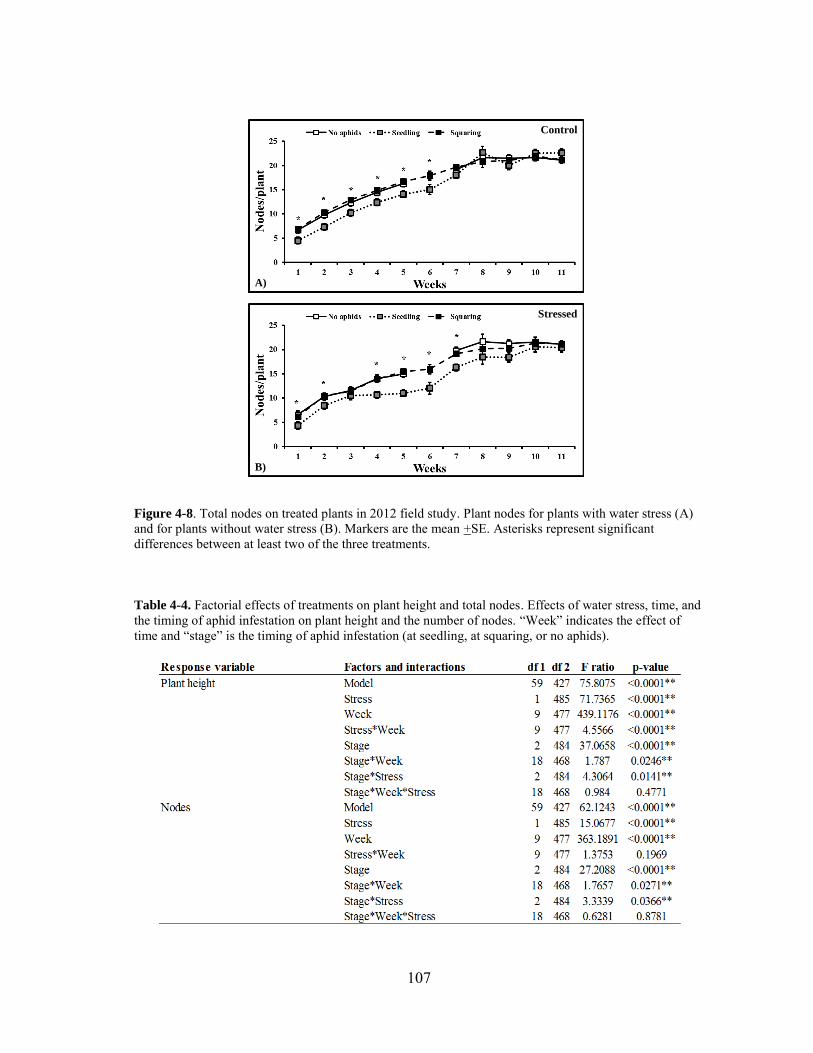
107

Figure 4-8. Total nodes on treated plants in 2012 field study. Plant nodes for plants with water stress (A) and for plants without water stress (B). Markers are the mean +SE. Asterisks represent significant differences between at least two of the three treatments. Table 4-4. Factorial effects of treatments on plant height and total nodes. Effects of water stress, time, and the timing of aphid infestation on plant height and the number of nodes. “Week” indicates the effect of time and “stage” is the timing of aphid infestation (at seedling, at squaring, or no aphids).

B)

A)

Control

Stressed

108

weeks four through seven (Fig. 4-8B). With the data pooled across all treatments, the

number of nodes was significantly affected by all factors and combinations except the

interaction between stress and week and the interaction between week, stress, and the

timing of aphid infestation (Table 4-4).

The timing of aphid infestation had no effect on the number of first position bolls

produced and had no effect on first position bolls on stressed plants. For control plants,

the timing of aphid infestation did not have an effect (stage: F2, 76= 0.66, p= 0.5158) and

the number of bolls were similar (Fig. 4-9A).

Figure 4-9. Number of 1st and 2nd position bolls on treated plants in 2012. 1st position bolls for plants with and without water stress (A) and for 2nd position bolls for plants with and without water stress (B). Bars are the mean +SE. Bars with letters of the same size were statistically compared and bars with different letters above them are significantly different.

B)

A)

1st Position

2nd

Position

109

Stressed plants were similar to control plants with the timing of aphid infestation

having no effect on the number of first position bolls produced (stage: F2, 76= 1.48, p=

0.2330) and the number of bolls were similar across the different timings of aphid

infestation (Fig. 4-9B). With pooled data, first position bolls (as well as all boll and lint

data) were analyzed for effects of stress, timing of aphid infestation, and the interaction

of stress and the timing of aphid infestation (no time comparison). First position bolls

were not significantly affected by any of the factors or interactions (Table 4-5).

Second position bolls on control plants were significantly affected by the timing

of aphid infestation, but stressed plants were unaffected. For control plants, the timing of

aphid infestation had an effect on the number of second position bolls (stage: F2, 76=

3.53, p= 0.0342) with plants infested with aphids during the seedling stage have 30%

more bolls than plants without aphids (Fig. 4-9B). For stressed plants, there was no

effect of timing of aphid infestation (stage: F2, 93= 1.77, p= 0.1761) and the number of

bolls were similar for all timings of aphid infestation (Fig. 4-9B). With pooled data,

second position bolls were significantly affected by the interaction of water stress and

the timing of aphid infestation (Table 4-5).

The timing of aphid infestation had different effects on the percent of bolls

unopened by the harvest date on October 12th, 2012 for control plants and stressed

plants. For control plants, the timing of aphid infestation did not have an impact on the

percent of bolls unopened (stage: F2, 76= 0.95, p= 0.3924) (Fig. 4-10A). For stressed

plants, the timing of aphid infestation had an effect (stage: F2, 93= 4.71, p= 0.0112) and

plants with aphids added during the seedling stage had 12% of their bolls unopened

110

compared to 4.5% for plants with no aphids and plants with aphids added during the

squaring stage (Fig. 4-10A). With pooled data, bolls unopened by harvest were

Table 4-5. Factorial effects of treatments on 1st and 2nd position bolls and lint. Effects of water stress, time, and the timing of aphid infestation on the number of bolls and lint yield. “Week” indicates the effect of time and “stage” is the timing of aphid infestation (at seedling, at squaring, or no aphids). ** indicates significance at 0.05 and * indicates marginal significance at 0.1

only affected by the interaction of stress and the timing of aphid infestation (Table 4-6).

Fruit retention was not affected by the timing of aphid infestation. For control

plants, the timing of aphid infestation did not have an effect (stage: F2, 200= 0.70, p=

0.4992) and fruit retention was similar among timings of aphid infestation (Fig. 4-10B).

For stressed plants, aphid infestation did not have an effect (stage: F2, 229= 1.28, p=

0.2805) and fruit retention was the same among aphid treatments (Fig. 4-10B). With

pooled data, fruit retention was marginally affected by water stress (Table 4-6).

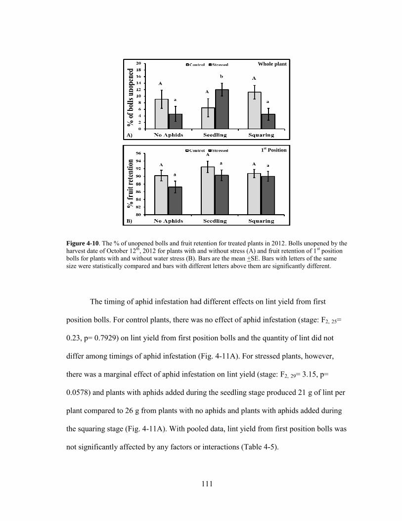
111

Figure 4-10. The % of unopened bolls and fruit retention for treated plants in 2012. Bolls unopened by the harvest date of October 12th, 2012 for plants with and without stress (A) and fruit retention of 1st position bolls for plants with and without water stress (B). Bars are the mean +SE. Bars with letters of the same size were statistically compared and bars with different letters above them are significantly different. The timing of aphid infestation had different effects on lint yield from first

position bolls. For control plants, there was no effect of aphid infestation (stage: F2, 25=

0.23, p= 0.7929) on lint yield from first position bolls and the quantity of lint did not

differ among timings of aphid infestation (Fig. 4-11A). For stressed plants, however,

there was a marginal effect of aphid infestation on lint yield (stage: F2, 29= 3.15, p=

0.0578) and plants with aphids added during the seedling stage produced 21 g of lint per

plant compared to 26 g from plants with no aphids and plants with aphids added during

the squaring stage (Fig. 4-11A). With pooled data, lint yield from first position bolls was

not significantly affected by any factors or interactions (Table 4-5).

B)

A)

1st Position

Whole plant

112

Lint yield from second fruiting positions was not affected by the timing of aphid

infestation, but there were differences between control and stressed plants. In control

plants, lint yield was not affected by the timing of aphid infestation (stage: F2, 28= 0.98,

p= 0.3862) and was similar among all timings of aphid infestation (Fig. 4-11B). For

stressed plants, the timing of aphid infestation also had no effect (stage: F2, 32= 1.19, p=

0.3178) and lint yield was similar among timings of aphid infestation (Fig. 4-11B). With

pooled data, however, lint yield from second fruiting positions was significantly affected

by water stress (Table 4-5).

Table 4-6. Factorial effects of treatments on % bolls unopened and retention. Effects of water stress and the timing of aphid infestation on % of bolls unopened by October 12, 2012 and % of bolls retained by the end of the season. “Week” indicates the effect of time and “stage” is the timing of aphid infestation (at seedling, at squaring, or no aphids). ** indicates significance at 0.05 and * indicates marginal significance at 0.1.

Total lint yield from all bolls on the cotton plant was not affected by the timing

of aphid infestation or water stress. For control plants, total lint yield was not affected by

the timing of aphid infestation (stage: F2, 27= 0.66, p= 0.5248) and there were no

differences in lint yield among the timings of aphid infestation (Fig. 4-12). For stressed

plants, lint yield was not affected by the timing of aphid infestation (stage: F2, 34= 1.05,

p= 0.3616) and there were no differences among timings of aphid infestation (Fig. 4-12).

113

With pooled data, total lint yield was not significantly affected by any factors or the

interaction of factors.

Characteristics of cotton quality (micronaire, strength, etc.) were similar between

plants regardless of the timing of aphid infestation and water stress. Micronaire (measure

of fineness and maturity), for instance, ranged between 4.5 to 4.9 with lower values

indicating higher cotton fineness and higher values indicating coarser fibers (Raskopf

1966, Montalvo Jr 2005) (Table 4-7). Plants without water stress had longer fibers

compared to stressed plants, with stress-free plants in the “long” fiber category and

stressed plants in the “medium-long” fiber category (Bradow and Davidonis 2000)

(Table 4-7). Cotton fiber uniformity varied between 82.5 and 84.2 with similar

uniformity indices between water stressed plants and plants with different timings of

aphid infestation. In addition, the strength of cotton fibers ranged from 27.9 (average) to

31.7 (very strong) and elongation of cotton fibers were similar among all treated plants

(Table 4-7) (Raskopf 1966, Montalvo Jr 2005, USDA 2005).

Table 4-7. Effects of treatments on cotton lint quality.

114

4.4 Discussion

Water stress had the strongest effects on cotton development and lint yield. In

general, the timing of aphid infestation significantly affected cotton development when it

was combined with water stress. The low impact of the timing of aphid infestation was

most likely due to a sharp and persistent decline in aphids during the first half of the

season, resulting in relatively low aphid herbivory as plants reached maturity. The sharp

decline in aphids and consistently low abundances on both stressed and control plants

while in enemy-free cages suggest that overcrowding or ontogenetic changes in plants

may have led to declines in aphid abundance (Boege and Marquis 2005). Previous

studies suggested that aphid abundance would vary on water-stressed plants and aphids

would decline over time. For instance, green spruce aphids (Elatobium abietinum)

feeding on pulse stressed and watered green spruce trees reached maximum abundances

of 90 and 68 aphids per tree, respectively, after 60 days of feeding on green spruce trees,

after which both treatments decreased to 32 and 10 aphids per tree over the next 30 days

(Major 1990). Furthermore, cotton aphids on six different, unstressed cotton cultivars

reached peak aphid densities of 300-350 aphids per leaf between 195-202 Julian days

(14-24 July), after which densities decreased to under 50 aphids for all six cultivars in

the next week (Weathersbee III and Hardee 1994). Even when plants were not stressed

(the latter example) aphids decreased in abundance on host plants, suggesting that other

factors aside from stress and plant cultivar dictate aphid abundance on host plants. In

addition, temperature may have influenced aphid abundance and led to declining aphid

populations. Aphid reproductive capacity decreases from 22 to 32°C (Slosser et al.

115

1989), while temperatures during week three and four of our study reached 31 to 39°C.

Various aspects of cotton ontogeny, temperature, and overcrowding may have

contributed to the decline and persistently low abundances of aphids; further

examination will be required to address the full extent of this phenomenon.

Water stress inconsistently affected concentrations of amino acids and digestible

carbohydrates and fluctuations in nutrients generally followed similar patterns regardless

of aphid infestation. When data was pooled, however, amino acids were significantly

affected by many factors, suggesting that the timing of aphid infestation and aphids over

time also have a strong influence on nutrient concentrations. Consequently, our results

do not follow the Plant Stress Hypothesis that suggested that water stress should increase

nutrient concentrations compared to unstressed plants (White 1969, Price 1991).

Unfortunately, aphid abundance was minimal during many of the instances in which

concentrations of amino acids differed between plants with different aphid infestation

times. During week three, however, when aphids were reached their greatest abundance

on plants with aphids added during the seedling stage, amino acids were at their highest

concentration, suggesting an interaction between aphid abundance and amino acids

(Figs. 4-2A and 4-3B). Despite this and other differences in amino acids in stressed

plants compared to control plants, aphids continued to decline in abundance. This is

further evidence suggesting that other factors besides nutrients in host plants influence

aphid abundance. Additionally, we did add lady bugs to cages to reduce populations due

to increasing cases of black sooty mold on honeydew. This, however, should not have

116

resulted in the collapse of colonies as the predators were only in the cages for three days

and removed afterwards, after which populations should have recovered.

Cotton plants with varying aphid infestation times and under stressed or stress-

free conditions did not vary in boll and lint production, suggesting that cotton

compensated or avoided the negative effects of these abiotic and biotic stresses. After

herbivory, plants in natural and agricultural systems have been known to compensate

(match the fitness of unconsumed plants) and even overcompensate (exceed the fitness

of unconsumed plants) for herbivore damage (Trumble et al. 1993, Strauss and Agrawal

1999, Wilson et al. 2003). Compensating plants regrow lost tissue, increase

photosynthetic rate, and/or reallocate photoassimilates to damaged tissue (Trumble et al.

1993, Sadras 1995). Additionally, cotton may completely compensate for aphid

herbivory during the pre-reproductive stages of plant growth and the timing of cotton

maturation, quantity of yield, and the quality of the fiber are unaffected (Rosenheim and

Wilhoit 1993, Rosenheim et al. 1997, Godfrey et al. 2000). For example, Rosenheim et

al. (1997) found that cotton plants with aphid herbivory were similar to aphid-free plants

six weeks after aphid populations declined. In addition, total above-ground biomass and

allocation of biomass to leaf, stem, and fruit production was similar between treatments.

In our study, cotton plants may have compensated for aphid herbivory within weeks

after the decline of aphid abundances. On the other hand, stressed plants may not have

been stressed long enough to induce boll shed and may have avoided production losses

due to stress rather than compensated for them. Cotton squares and bolls are primarily

affected by impaired photosynthesis, while photosynthesis may be maintained or

117

actually increase with initial water stress and functionally supported by stress-related

nutrients and compounds (Guinn and Service 1982, Chaves et al. 2003, Jithesh et al.

2006, Taiz and Zeiger 2010). Squares and bolls, however, are sensitive to the loss of

photoassimilates from nearby source leaves, in which the abscission of younger squares

and bolls may occur (Guinn and Service 1982, Freeland et al. 2006). It may have been

possible, therefore, that the water stress our plants experienced was not severe enough to

induce boll shed in our plants (-1.24 MPa, Fig. 4-1). Furthermore, antioxidant enzymes

such as peroxidase migrate from leaves to squares and bolls when plants become water

stressed (Sandhu et al. 2007), which may support why peroxidase activity declined in the

leaves of stressed plants compared to stress-free control plants (Fig. 4-6A). Cotton

plants, therefore, demonstrated several physiological mechanisms that allowed for the

compensation of aphid herbivory and avoidance of stress-induced fruit shed, resulting in

similar lint production and quality between treatments.

Our study illustrated that aphid infested and water-stressed cotton plants may

produce comparable lint yields to uninfested plants. Aphid abundance may be more

influenced by ontogenetic and abiotic factors than stress-induced changes in host plants,

resulting in early season population declines in enemy-free space. Future work would

need to address the extent to which aphid population dynamics depend upon ontogenetic

changes in host plants, and the degree to which allelochemistry and resource allocation

in host plants play a role. In addition, increasing the severity and frequency of water

stress may more thoroughly address how water stress and ontogenetic changes in plants

influence aphid abundance and subsequent lint yield. Our study is one of the first to

118

address the combined effects of the timing of aphid infestation and water stress,

however, more research needs to be done further explore the complexity of these

interactions.

119

CHAPTER V

THE NUTRIENT AVAILABILITY HYPOTHESIS: DEVELOPMENT OF A

UNIFYING PLANT STRESS-HERBIVORE HYPOTHESIS

5.1 Introduction

There has been a long-standing interest in accurately predicting the effects of

water deficit stress on plant-insect interactions (Loomis 1932, White 1969, Coley et al.

1985, Herms and Mattson 1992, Koricheva et al. 1998, Huberty and Denno 2004, Jactel

et al. 2012). Over 500 published studies have addressed this topic (search results from

the Web of Knowledge and Google Scholar 2013) and nearly half a dozen formal

hypotheses have been developed to explain the effects of water deficit stress on insect

herbivores (Loomis 1932, White 1969, Coley et al. 1985, Price 1991, Huberty and

Denno 2004). Despite this intensive effort, it is still difficult to accurately predict the

effects of water deficit stress on insect abundance and performance. Some studies, for

example, have found that insect herbivores including gall midges (Diptera:

Cecidomyiidae), inchworms (Lepidoptera: Geometridae), and aphids (Hemiptera:

Aphididae) perform better and are more abundant on water deficit-stressed plants

(Waring and Price 1990, Archer et al. 1995, Schowalter et al. 1999). Other studies,

however, have shown that these same insects or their close relatives perform better and

are more abundant on non-stressed plants (Hanks and Denno 1993, Larsson and

Bjorkman 1993, Inbar et al. 2001). Variable results such as these are extremely common

in the literature, so understanding the sources that contribute to variation in the effects of

120

water deficit stress on plant-insect interactions is of vital importance to the management

of agricultural and natural ecosystems. Climate change predicts more intense and

frequent droughts, which makes it even more critical that we understand the factors that

determine the impact of water deficit stress on plant-insect interactions (Dai 2011, Kiem

and Austin 2013, Van Lanen et al. 2013).

Water deficit stress can be broadly defined as alterations in normal plant

functions and physical-chemical equilibrium due to water deficit (Bray 1997, Shao et al.

2008), leading to alterations in how plants manage water, hormones, enzymes, and

macro- and micronutrients (Hsiao 1973, Herms and Mattson 1992, Chaves et al. 2002,

Chaves et al. 2003, Hu et al. 2006, Jithesh et al. 2006, Shao et al. 2008, Taiz and Zeiger

2010). Predicting the impacts of water deficit stress on herbivore performance is difficult

because stress changes plant physiology in ways that can increase primary metabolites

(macronutrients) and secondary metabolites (toxic allelochemicals) in host plants.

During water stress, plants accumulate macronutrients and antioxidant enzymes to

alleviate the deleterious effects of stress (White 1969, English-Loeb et al. 1997, Sholwer

2002, Huberty and Denno 2004, Jithesh et al. 2006, Ghannoum 2008, Mody et al. 2009).

These compounds stabilize cell membranes, cytoplasmic enzymes, and scavenge free

radicals (Jithesh et al. 2006, Parida et al. 2008, Taiz and Zeiger 2010). The accumulation

of macronutrients, however, can be beneficial to herbivores because they contain amino

acids and essential nutrients for insect growth and development. For example, the

concentration of the amino acid phenylalanine increases in stressed plants and is

required for insects to synthesize tyrosine to stabilize and pigment cuticle and form

121

proteinaceous structures (Kramer and Hopkins 1987, Daubner et al. 2011, Vavricka et al.

2014) . Water stress, however, can also lead to tougher leaves, more trichomes, thicker

surface waxes, and possibly higher concentrations of toxic secondary metabolites that all

negatively affect herbivores (Raupp 1985, Herms and Mattson 1992, Stamp 2003).

Focusing on stress-induced changes in plants may provide an objective, mechanistic

basis for predicting herbivore performance on water deficit-stressed plants by

concentrating on the changes in plant physiology that directly influence herbivore

performance.

In addition, most studies tend to generalize the effects of water deficit stress on

macronutrients and allelochemicals across plant taxa, ignoring potential inherent

differences among plants (Coley et al. 1985, Price 1991, Huberty and Denno 2004, Jactel

et al. 2012). Variation in herbivore response to stressed plants may arise due to intrinsic

differences in how different plants allocate macronutrients and allelochemicals in

response to water stress. Any assessment of the effects of water deficit stress on plant-

insect interactions should explicitly address potential variation among plant groups.

The goal of this meta-analysis was to determine the relationship between stress-

induced changes in water deficit-stressed plants and herbivore performance. Specifically,

we determined: 1) how concentrations of key macronutrients and allelochemicals in

plants change during water stress, 2) the performance of herbivores on water-stressed

plants, 3) the relationship between stress-induced changes in plant macronutrients,

allelochemicals, and herbivore performance, and 4) variation among plant taxa and the

effects of water stress on concentrations of macronutrients and allelochemicals. The

122

analysis included studies that reported changes in plant macronutrients and

allelochemicals in water-stressed plants in addition to herbivore performance (e.g.,

growth, survival, etc.). Our approach was novel in that it specifically focused on

potential mechanisms that influence herbivore performance on water-stressed plants by

directly examining stress-induced changes in plants and the correlated changes in

herbivore response.

5.2 Methods

5.2.1 Selection criteria for meta-analysis

We selected experimental and observational studies from 1967 (the earliest study

we found) to 2013 that examined the influence of water deficit stress on macronutrients,

allelochemicals, and herbivore performance. Macronutrients from selected studies were

compounds that can be beneficial to herbivore growth and development, including plant

primary metabolites, amino acids, proteins (excluding defensive proteins), and digestible

carbohydrates. Allelochemicals from selected studies were any secondary metabolites

produced by the plant that could negatively affect herbivore growth and development

such as phenolics, alkaloids, terpenes, etc. Herbivore performance from selected studies

referred to individual herbivore growth, development, survival, and as well as population

growth. Our literature search used the Web of Knowledge and Google Scholar

databases, and phrases such as “water stress and insects”, “plant stress and nutrients”,

and “plant stress and insects”. We also searched the literature cited from all published

studies that we selected. Studies were excluded if they: 1) did not include a well-watered

123

or stress-free control, 2) implemented water stress without water deficit (e.g., root

excision, polyethylene glycol), or 3) lacked the statistical information required for a

meta-analysis (i.e., sample size, standard error). Studies included in our meta-analysis

did not have plants that were primed for water deficit stress (exposed to water deficit

stress prior to study).

5.2.2 Meta-analysis

Changes in macronutrients, allelochemicals, and herbivore performance between

control and water deficit-stressed plants were collected from published studies using

Grab It! Software (Datatrend Software, 1998-2001) and analyzed using MetaWin 2.0

(Rosenberg et al. 1997). Observations of changes included differences between

concentrations of individual macronutrients and allelochemicals between control and

water deficit-stressed plants. For example, if a study reported changes in the

concentration of the amino acids glutamine, methionine, and phenylalanine, those three

differences were counted as individual observations for changes in macronutrients, not

averaged and counted as a single observation. Amino acids and other macronutrients are

used differently by plants and insects (Chapman 1998, Taiz and Zeiger 2010), thus

averaging the changes in concentrations of individual amino acids into a single number

may underestimate the degree of change that occurs within plants and the implications

those changes have for plant and insect growth and development (e.g., essential versus

non-essential amino acids). Treating differences between individual amino acids as

124

individual observations is an inclusive way to highlight the biological significance of

changes in macronutrients and nutrient profiles in water-stressed plants.

We estimated effect size by calculating Hedge's d, which measured the

magnitude of effect that a treatment had on an experimental unit versus the effect of the

control. An effect size of "0" (95% CI includes zero) meant that the treatment had the

same effect as the control and differences in effect sizes indicate differences in the

magnitude of change. The meta-analytical program MetaWin 2.0 was used to calculate

Hedge’s d which accounts for differences in sample sizes and weights categorical

responses according to sample size (Rosenberg et al. 1997). Weighted values are added

to each analysis based on the differences between sample sizes, the total variance of

categorical data, and estimated with a 95% CI. Hedge’s d values are compared similarly

to ANOVA and between-group heterogeneity (QB) was tested against a chi-square

distribution to determine if significant differences exist between groups of categorical

variables (Rosenberg et al. 1997, Kaplan and Denno 2007). A minimal effect size ranges

from +0.1-0.3, a moderate effect from +0.3-0.7, and a large effect size is a value larger

than +0.7. In our analyses, we searched for relationships between changes in plant

chemistry (e.g., macronutrients, allelochemicals) and herbivore response in various

taxonomic groups for plants and insects (including feeding guild and diet breadth for

insects). To determine the influence of water deficit stress on different macronutrients in

the analyses, we divided “macronutrients” into “total macronutrients” (amino acids,

proteins, digestible carbohydrates, including nitrogen), “nitrogenous macronutrients”

(amino acids, proteins, including nitrogen), and “digestible carbohydrates” (sugars).

125

Herbivore performance data was pooled and analyzed as “performance” due to

insufficient data to analyze each measurement individually (survivorship compared to

fecundity, etc.). In addition, we compared concentrations of macronutrients and

allelochemicals in stressed plants that either increased or decreased herbivore

performance. For these analyses, we analyzed data from studies with data on

macronutrients, allelochemicals, and herbivore performance. Effect sizes were reported

using the between-group heterogeneity test statistic (QB), the p-value from the test

against the chi-square distribution, and the mean effect size + a 95% confidence interval.

5.3 Results

5.3.1 Plant responses to water deficit stress

We found 42 published studies that met our selection criteria for the meta-

analysis. For the analysis of stress-induced changes in total macronutrients, 11 plant taxa

were sufficiently represented in the data to be analyzed. Water deficit stress affected

concentrations of total macronutrients (QB= 412.06, p<0.0001, df= 10, N= 634; Fig. 5-1)

and led to increases in 8 of the 11 plant taxa. Plants in the family Malvaceae greatly

increased total macronutrients with an effect size of 0.97+0.06, followed by plants in the

family Brassicaceae (0.69+0.30). Furthermore, plants in the families Betulaceae,

Poaceae, and Salicaceae moderately increased concentrations of total macronutrients

(Betulaceae: d= 0.45+0.31, n= 10; Poaceae: d= 0.34+0.08, n= 127; Salicaceae: d=

0.32+0.16, n= 24; Fig. 1) and plants in the families Solanaceae and Rutaceae increased

126

concentrations minimally (Solanaceae: d= 0.24+0.22, n= 29; Rutaceae: d= 0.12+0.11, n=

147; Fig. 5-1).

Figure 5-1. Total macronutrients in stressed plants by plant taxa. Mean effect size + 95% CI. Numbers above bars indicate the number of observations per plant taxa.

Ten plant taxa were sufficiently represented in the data to be analyzed for stress-

induced changes in nitrogenous macronutrients and there was significant variation in the

effects of water deficit stress among plant taxa (QB= 379.33, p<0.0001, df= 9, N= 546;

Fig. 5-2A). In 7 of the 10 plant taxa, concentrations of nitrogenous macronutrients

increased. There were very large increases in plants from Malvaceae and Brassicaceae

(Malvaceae: d= 0.96+0.06, n= 167; Brassicaceae: d= 0.96+0.30, n= 23; Fig. 5-2A). In

addition, plants in the families Fabaceae and Betulaceae increased concentrations of

nitrogenous macronutrients moderately (Fabaceae: d= 0.63+0.22, n= 26; Betulaceae: d=

127

0.45+0.31, n= 10; Fig. 5-2A) and plants in the families Pinaceae and Rutaceae increased

concentrations minimally (Pinaceae: d= 0.12+0.14, n= 49; Rutaceae: d= 0.12+0.11, n=

147; Fig. 5-2A).

Concentrations of digestible carbohydrates were analyzed for 7 plant taxa and

stress-induced changes varied among plants (QB= 27.37, p= 0.0012, df= 6, N= 91; Fig.

5-2B). Water deficit stress significantly increased digestible carbohydrates in 3 of the 7

plant taxa. Salicaceae and Cucurbitaceae plants increased carbohydrates the greatest in

response to water deficit stress (Salicaceae: d= 0.91+0.58, n= 6; Cucurbitaceae: d=

0.87+0.65, n= 5), while four plant taxa exhibited no change (Fig. 5-2B). For instance,

Figure 5-2. Nitrogenous macronutrients and digestible carbohydrates. The effects of water deficit stress on nitrogenous macronutrients (A) and digestible carbohydrates (B) in different plant families. Mean effect size + 95% CI. Numbers above bars indicate the number of observations per plant taxa. in one of the studies in our analysis, water deficit-stressed Populus spp. (Salicaceae)

increased sucrose concentrations by 450% compared to unstressed Populus spp

128

(Tschaplinski and Blake 1989).

Stress-induced changes in allelochemicals were analyzed for five plant taxa that

were sufficiently represented in the data to be analyzed. Water deficit stress significantly

varied concentrations of allelochemicals among plants (QB= 35.14, p<0.0001, df= 4, N=

288; Fig. 5-3) and led to increases in 3 of the 5 plant taxa. Plants in the Solanaceae

increased allelochemicals the most in response to water deficit stress (d= 0.39+0.17, n=

48) followed by plants in Ericaceae, while plants in Pinaceae and Salicaceae exhibited

no change (Fig. 5-3). For example, in one of the studies in our analysis, water deficit-

stressed Calluna vulgaris (Ericaceae) increased anthocyanins by 30% compared to

unstressed C. vulgaris (Bucchetti et al. 2011).

Figure 5-3. Allelochemicals in stressed plants by plant taxa. Mean effect size + 95% CI. Numbers above bars indicate the number of observations per plant taxa.

129

5.3.2 Herbivore response to water-stressed plants

Herbivore response to water deficit-stressed plants was analyzed for six

herbivore taxa that were sufficiently represented in the data to be analyzed (Fig. 5-4).

Herbivore performance was significantly affected on stressed host plants and

performance varied among herbivore taxa (QB= 162.47, p<0.0001, df= 5, N= 171; Fig.

5-4). Grasshoppers (Orthoptera: Acrididae) increased their performance the most, with a

large, positive response to water deficit-stressed plants (d= 0.73+0.17, n= 7) followed by

cabbage butterflies (Lepidoptera: Pieridae, d= 0.51+0.39, n= 6) and decreased

performance from aphids (Hemiptera: Aphididae, d= -0.37+0.16, n= 40) (Fig. 5-4). For

example, in one of the studies in our analysis, green apple aphids (Hemiptera: Aphis

pomi) decreased in abundance by 82% on water-stressed apple trees (Rosaceae: Malus

domestica) compared to green apple aphids on unstressed apple trees (Mody et al. 2009).

Figure 5-4. Herbivore performance on stressed plants by herbivore taxa. Mean effect size + 95% CI. Numbers above bars indicate the number of observations per herbivore taxa.

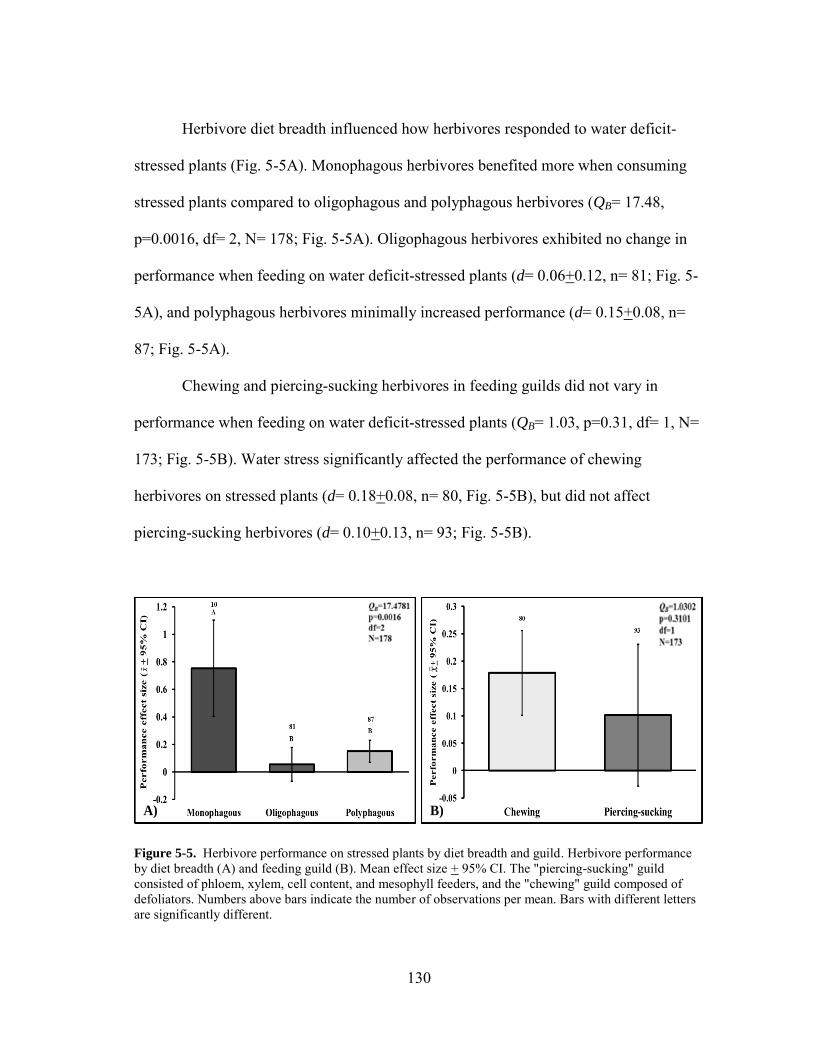
130

Herbivore diet breadth influenced how herbivores responded to water deficit-

stressed plants (Fig. 5-5A). Monophagous herbivores benefited more when consuming

stressed plants compared to oligophagous and polyphagous herbivores (QB= 17.48,

p=0.0016, df= 2, N= 178; Fig. 5-5A). Oligophagous herbivores exhibited no change in

performance when feeding on water deficit-stressed plants (d= 0.06+0.12, n= 81; Fig. 5-

5A), and polyphagous herbivores minimally increased performance (d= 0.15+0.08, n=

87; Fig. 5-5A).

Chewing and piercing-sucking herbivores in feeding guilds did not vary in

performance when feeding on water deficit-stressed plants (QB= 1.03, p=0.31, df= 1, N=

173; Fig. 5-5B). Water stress significantly affected the performance of chewing

herbivores on stressed plants (d= 0.18+0.08, n= 80, Fig. 5-5B), but did not affect

piercing-sucking herbivores (d= 0.10+0.13, n= 93; Fig. 5-5B).

Figure 5-5. Herbivore performance on stressed plants by diet breadth and guild. Herbivore performance by diet breadth (A) and feeding guild (B). Mean effect size + 95% CI. The "piercing-sucking" guild consisted of phloem, xylem, cell content, and mesophyll feeders, and the "chewing" guild composed of defoliators. Numbers above bars indicate the number of observations per mean. Bars with different letters are significantly different.

A) B)

131

5.3.3 Macronutrients, allelochemicals, and herbivore performance

Across all 42 studies, water deficit stress significantly increased concentrations

of total macronutrients and allelochemicals in plants, with greater increases in total

macronutrients than allelochemicals (QB= 137.07, p<0.0001, df= 1, N= 935; Fig. 5-6).

Concentrations of total macronutrients increased twice as much as allelochemicals in

water deficit-stressed plants (total macronutrients: d= 0.54+0.04, n= 641 and

allelochemicals: d= 0.24+0.03, n= 294; Fig. 5-6).

Figure 5-6. Total macronutrients and allelochemicals in stressed plants. Mean effect size + 95% CI. Numbers above bars indicate the number of observations.

We found strong evidence that stress-related changes in total macronutrients

were the most important factors in determining herbivore performance on water deficit-

stressed plants. Concentrations of total macronutrients significantly differed between

132

stressed plants that increased or decreased herbivore performance (QB= 41.43, p<0.0001,

df= 1, N= 343; Fig. 5-7). Water deficit-stressed plants with moderate to large increases

in concentrations of total macronutrients increased herbivore performance (d=

0.46+0.08, n= 76; Fig. 5-7). In contrast, herbivores decreased performance on stressed

plants with a minimal increase in total macronutrients (d= 0.19+0.04, n= 267; 5-7). On

the other hand, concentrations of allelochemicals in stressed plants were not associated

with changes in herbivore performance (QB= 0.56, p=0.46, df= 1, N= 76; increased

performance: d= 0.11+0.16, n= 62; decreased performance: d= 0.21+0.21, n= 14; Fig. 5-

7).

Figure 5-7. Bicoordinate plot with herbivore performance by macronutrients and allelochemicals. A comparison of the concentrations of macronutrients and allelochemicals in water deficit-stressed plants that either decreased herbivore performance (black circle) or increased herbivore performance (white circle). The x-axis is the effect size of macronutrients and the y-axis is the effect size of allelochemicals. The circles are mean effect size + 95% CI. Numbers above CI intervals indicate the number of observations. Macronutrients: QB= 41.43, p<0.0001, df= 1, N= 343; Fig. 9A), allelochemicals: QB= 0.56, p=0.46, df= 1, N= 76.

133

5.4 Discussion

Our analysis provided strong evidence that stress-induced increases in host plant

macronutrients determine herbivore performance on water deficit-stressed plants. Based

on this result, we propose the Nutrient Availability Hypothesis (NAH), which predicts

that changes in the concentration of macronutrients are the most important factor in

determining herbivore abundance on water deficit-stressed plants and, conversely, that

changes in allelochemicals are not important. This hypothesis is novel because it focuses

on stress-induced changes in macronutrients as the mechanism driving insect herbivore

performance and abundance on water deficit-stressed plants. In addition, our hypothesis

incorporates the predictions of other plant-insect herbivore hypotheses. The Plant Stress

Hypothesis predicts that herbivores will outbreak on water stressed plants due to

increased foliar nitrogen (White 1969). Research since White developed this hypothesis,

however, has shown that not all insect herbivores outbreak on water deficit-stressed

plants. The Nutrient Availability Hypothesis expands this idea not only to take into

account variation among different plants in their response to water deficit stress, but our

associated meta-analysis also indicates that stress-induced changes in carbohydrates and

not just changes in nitrogen are responsible for changes in herbivore performance.

The Growth-Differentiation Balance Hypothesis (GDBH) predicts that plants

growing in resource-poor conditions (e.g., water deficit limiting carbon uptake) will

have increased allelochemicals and overall plant defense as a strategy to reduce resource

demand for regrowth due to herbivory (Coley et al. 1985, Lorio Jr 1986, Fajer et al.

1992, Herms and Mattson 1992, Fine et al. 2004). Furthermore, the GDBH predicts that

134

the defensive strategies resource-limited plants employ may be linked to their

evolutionary and life history, leading to differences in macronutrient allocation and plant

defense between plant taxa under similar environmental conditions (Coley et al. 1985,

Ryser and Lambers 1995, Fine et al. 2004). Our meta-analysis strongly suggests that

water stress-induced changes in allelochemicals are relatively unimportant, thus NAH

focuses on stress-induced changes in nutrients. The simple predictive nature of NAH

may be applied across host plants regardless of the magnitude of stress in their

evolutionary history.

Our study was the first comprehensive assessment of how water stress-induced

changes in macronutrients and allelochemicals affect herbivore performance. Previous

reviews of herbivore performance on water deficit-stressed plants focused on differences

between herbivore feeding guilds and often focused on a specific plant taxa or group of

plants (e.g., forest species, woody plants) (Mattson and Haack 1987, Price 1991,

Koricheva et al. 1998, Huberty and Denno 2004, Cornelissen et al. 2008, Jactel et al.

2012). Inherent differences among plants may be an underlying cause for the

inconsistencies observed in studies of interactions between water deficit-stressed plants

and herbivores. We found significant variation in the magnitude of change in

macronutrients and allelochemicals among 11 plant taxa with different evolutionary

histories (Figs. 5-1 and 5-2). This suggests that water deficit stress may induce changes

in the concentration of macronutrients and allelochemicals in inherently different ways

in different plant taxa. Few studies have directly examined or reported the differences

between multiple plant taxa (i.e., plant family) in response to water stress. These few

135

studies outside our meta-analysis illustrate that various plant taxa respond differently to

water stress (Nash and Graves 1993, Koricheva et al. 1998, Durhman et al. 2006). For

example, water deficit-stressed Acer rubrum (Aceraceae) had a 50% greater net

assimilation rate of carbon compared to that of water deficit-stressed Asimina triloba

(Annonacea) and 30% greater compared to that of water-deficit stressed Nyssa sylvatica

(Cornaceae) (Nash and Graves 1993). In addition, Sedum acre, S. kamtschaticum, and S.

reflexum (Crassulaceae) produced significantly more biomass during water deficit stress

compared to stressed grass and aster species (Asteraceae) (Durhman et al. 2006). These

studies did not report differences in macronutrients or allelochemicals, but differences in

net assimilation rate and total biomass between different plant taxa during water deficit

stress suggest that there are substantial physiological differences among plants while

stressed. These physiological differences may contribute to differences in macronutrient

and allelochemical concentrations in stressed host plants, effectively increasing variation

in herbivore response.

In conclusion, we found that stress-induced changes in concentrations of

macronutrients were key in determining herbivore performance on water deficit-stressed

plants. We propose the Nutrient Availability Hypothesis which predicts that changes in

concentrations of macronutrients will determine herbivore performance on water deficit-

stressed plants. We believe focusing on stress-induced changes in macronutrients will

greatly improve our ability to accurately predict plant stress-herbivore interactions.

136

Au

tho

r(s

)T

re

atm

en

t(s)

Macro

nu

trie

nts

Alle

loch

em

icals

Am

undson et al. 1993W

ater stressG

eneral sugar content---

Barnett and N

aylor 1966Severe and m

oderate water stress

Am

ino acids, protein---

Baskin and B

askin 1974W

ater and pulsed water stress

Am

ino acids---

Bjorkm

an 2000W

ater stress---

Phenolic R

T40, phenolics

Bucchetti et al. 2011

Water stress

---A

nthocyanins, tanninsC

roise and Lieutier 1993

Water stress

Carbohydrates

---E

nglish-Loeb et al. 1997

Water stress for 2-14 days

Total N

, carbohydratesP

roteinase inhibitor, chlorogenic acid, rutinFranzke and R

einhold 2011W

ater stressA

mino acids, protein

---G

riffin et al. 1991W

ater stressA

mino acids

---G

uehl et al. 1992W

ater stressC

arbohydrates---

Gutbrodt et al. 2011

High and low

water stress

Nitrogen

Glucosinolates, alliarinoside, isovitexin

Hale et al. 2003

Water stress

Am

ino acids---

Hare et al. 1989

Water stress

Am

ino acids, protein, total nitrogen---

Inbar et al. 2001W

ater stressN

itrogen, carbonC

hitinase, glucanase, peroxidase, phenolicsIsaacs et al. 1998

Water stress

Am

ino acids, carbohydrates---

Joern and Mole 2005

Water stress

Nitrogen, carbohydrates

---K

ainulainen et al. 1992W

ater stress---

Terpenes

Khan et al. 2010

Water stress

Carbohydrates

---K

oppenaal et al. 1991W

ater stressed roots and shootsC

arbohydrates, nitrogen---

Lehto 1992

Water stress

Nitrogen

---M

cQuate and C

onnor 1990W

ater stressA

mino aicds

---M

eyer et al. 2006W

ater stressC

arbohydrates, proline---

Miles et al. 1982

Water stress

Am

ino acids, carbohydrates, nitrogenP

henolicsM

iles, Aspinall, R

osenberg 1982W

ater stressA

mino acids, carbohydrates

Phenolics

Mody et al. 2009

High and low

water stress

Nitrogen

---P

ritchard et al. 1997W

ater stress---

Phenolics, tannins

Roth et al. 1997

Water stress

Nitrogen, protein, carbohydrates

Tannins

Sadras et al. 1998W

ater stressN

itrogen---

Scheirs and Bruyn 2005

High, m

oderate, and low w

ater stressA

mino acids, protein

---Show

ler 2002Severe to low

water stress

Am

ino acids---

Showler and M

oran 2003H

igh to low w

ater stressA

mino acids

---Stew

art and Lieffers 1993

Water stress

Nitrogen, m

inerals, carbohydrates, amino acids

---T

alhouk et al. 1990W

ater stressSucrose

---T

ariq et al. 2011H

igh, moderate, low

water stress

Nitrogen, carbon

Glucosinolates

Tariq et al. 2013

High and m

oderate water stress

Nitrogen

Glucosinolates

Thom

as and Hodkinson

Low

water stress

Nitrogen

---T

schaplinski and Blake 1989

Water stress

Carbohydrates

---T

urtola et al. 2005W

ater stress---

Salicylates, flavinoids, chlorogenic acidsW

aring 1988H

igh and moderate w

ater stressP

roteinP

henolsW

aring and Price 1990

Water stress

Protein, nitrogen

Phenolic resin

Wellburn et al. 1996

Water stress

Protein, nitrogen

Phenols

Young and H

all 1986W

ater stressP

rotein---

137

Ho

st P

lan

t Fam

ilyH

erb

ivo

re

sp

ecie

sH

erb

ivo

re

(Fam

ily: O

rd

er)

Pinaceae

------

Poaceae

------

Legum

inosae---

---P

inaceae---

---E

ricaceae---

---P

inaceae---

---S

olanaceaeS

podoptera exiguaN

octuidae: Lepidoptera

Poaceae, F

abaceaeC

horthippus biguttulus A

crididae: Orthoptera

Salicaceae

------

Pinaceae

------

Brassicaceae

Pieris brassicae, S

podoptera littoralisP

ieridae, Noctuidae: L

epidopteraP

oaceaeR

hopalosiphum padi

Aphididae: H

emiptera

Rutaceae

Panonychus citri

Tetranychidae: T

rombidiform

esS

olanaceaeB

emisia argentifolii; L

iriomyza trifolii; H

eliothis zeaA

leyrodidae: Hem

iptera; Agrom

yzidae: Diptera; N

octuidae: Lepidoptera

Cucurbitaceae

Bem

isia tabaciA

leyrodidae: Hem

ipteraP

oaceae---

---P

inaceae---

---B

rassicaceaeM

yzus persicaeA

phididae: Hem

ipteraP

inaceae---

---P

inaceae---

---F

abaceae---

---P

iperaceaeA

tta colombica

Form

icidae: Hym

enopteraB

rassicaceae, Myrtaceae

Pieris rapae, P

aropsis atomaria

Pieridae: L

epidoptera; Chrysom

elidae: Coleoptera

Brassicaceae

Brevicoryne brassicae

Aphididae: H

emiptera

Rosaceae

Spodoptera exigua, A

phis pomi

Noctuidae: L

epidoptera; Aphididae: H

emiptera

Pinaceae

------

Salicaceae

Malacosom

a disstriaL

asiocampidae: L

epidopteraM

alvaceaeT

etranychus urticaeT

etranychidae: Trom

bidiformes

Poaceae

Chrom

atomyia m

iliiA

gromyzidae: D

ipteraM

alvaceae---

---M

alvaceaeS

podoptera exiguaN

octuidae: Lepidoptera

Pinaceae

------

Betulaceae

Lym

antria dispar L

ymantriidae: L

epidopteraB

rassicaceaeB

revicoryne brassicae, Myzus persicae

Aphididae: H

emiptera

Brassicaceae

Brevicoryne brassicae, M

yzus persicaeA

phididae: Hem

ipteraS

alicaceae, Betulaceae

------

Salicaceae

------

Salicaceae

------

Salicaceae

Euura lasiolepis

Tenthredinidae: H

ymenoptera

Zygophyllaceae

Asphondylia spp

Cecidom

yiidae: Diptera

Pinaceae

------

Ulm

aceaeX

anthogaleruca luteolaC

hrysomelidae: C

oleoptera

138

Die

t B

re

ad

th

Gu

ildP

erfo

rm

an

ce

Effe

ct o

n H

erb

ivo

re

Pe

rfo

rm

an

ce

------

------

------

------

------

------

------

---(-)

------

------

------

------

Polyphagous

Chew

ingG

rowth, survivorship

(-)P

olyphagousC

hewing

Grow

th, fecundity(+

)---

------

------

------

---M

onophagous, polyphagousC

hewing

Developm

ent, growth

(+) (-)

Polyphagous

Piercing-sucking

Population grow

th(-)

Oligophagous

Piercing-sucking

Egg production, density

(+) (-)

Polyphagous

Piercing-sucking, chew

ing, chewing

Egg production, grow

th(-)

Polyphagous

Piercing-sucking

Weight

(-)---

------

(-)---

------

---P

olyphagousP

iercing-sucking---

(+)

------

------

------

------

------

------

Polyphagous

Chew

ing---

(+)

Polyphagous, oligophagous

Chew

ingP

upae weight

(+)

Oligophagous

Piercing-sucking

---(+

)P

olyphagousC

hewing, piercing-sucking

Grow

th, abundance(-)

------

------

Polyphagous

Chew

ingG

rowth, developm

ent(-)

Polyphagous

Piercing-sucking

Fecundity, abundance

(-)O

ligophagousM

iner---

(-)---

------

---P

olyphagousC

hewing

Fecundity, grow

th, development

(-)---

------

---P

olyphagousC

hewing

Grow

th(+

) (-)O

ligophagous, polyphagous---

Fecundity, population grow

th(+

)---

---F

ecundity, population growth

(+)

------

---(+

)---

------

------

------

---M

onophagousG

allerS

urvivorship(-)

---G

aller---

(+)

------

------

Oligophagous

Chew

ingD

evelopment, fecundity

(+)

139

CHAPTER VI

CONCLUSION

Variation in herbivore response to water deficit-stressed plants can be

contributed to differences in the effects of pulsed and continuously stress, to differences

in herbivore response to these plants, due to interactions between the timing of herbivory

and plant development, and variation in the stress-induced changes in stressed plants in

not only cotton, but across plant taxa. I found that there were significant physiological

differences in the effects these different stress types had on cotton plants (Chapter II).

Furthermore, these physiological differences were not always consistent, but ultimately

increased the abundance of different herbivores who fed on these plants (Chapter III). In

addition, the interactions between the timing of herbivory and plant development

differentially affected aphid abundance, the duration of aphid feeding on stressed plants,

and cotton development (Chapter IV). Finally, stress-induced changes in water deficit-

stressed plants, primarily changes in macronutrients, were the most important factor in

determining herbivore performance on stressed plants (Chapter V).

Pulsed and continuous stress had different impacts on photosynthesis, stomatal

conductance, transpiration efficiency, plant development, and slight differences in

nutrients. This suggests that we need to consider the effects of stress severity and

frequency when predicting herbivore response to stressed plants. These developmental

differences in stressed plants will determine the amount of plant material herbivores

have to consume through significant changes in plant physiology and development such

140

as through changes in metabolic requirements of CO2 (Ort et al. 1994, Chaves et al.

2002, Taiz and Zeiger 2010), overall plant height, leaves, and lower water content which

would impede the feeding of PS and chewing herbivores (Wearing 1972, Scriber 1977,

Huberty and Denno 2004, Douglas 2006). In my dissertation, however, we did not find

consistent differences in concentrations of amino acids and digestible carbohydrates and

could not support the nutritional predictions of the PSH and PLSH hypotheses. I do

believe that the -1.2 MPa may not have been severe enough of a water stress to induce

enough differentiation of stress types. Based on my results from Chapter II, I would

conclude that herbivores may be responding to other factors aside from nutrients that

may influence their abundance, however, this conflicts with the results from my meta-

analysis (Chapter IV). Indeed, there were not clear differences in nutrients during my

three field studies from 2010-2012, but perhaps the studies in my meta-analysis induced

enough stress to make significant differences between stressed and unstressed plants to

provide the evidence I needed to develop my NAH hypothesis. In the future, I will

increase the amount of stress to ensure that there are strong differences between stressed

and unstressed plants. Despite this, I still demonstrated differences in herbivore response

to stressed plants.

In Chapter III I demonstrated clear differences in how herbivores respond to

pulsed and continuously stressed plants. Herbivores such as thrips, stink bugs,

fleahoppers, and whiteflies were more abundant on pulsed stressed plants compared to

continuously stressed plants. Aphids, however, were more sensitive to possibly

ontological and developmental changes in plants aside from water stress, but were

141

significantly associated with stress-induced changes in nutrients, however, this could not

been supported in Chapter IV. Furthermore, very few studies have compared the effects

of pulsed and continuous water stress on herbivores (Lightfoot and Whitford 1987,

Schowalter et al. 1999), but these few studies find various effects of stress on herbivore

abundance from the same feeding guild and even the same species having contrasting

responses to different stressed plants or even plants from the same taxa (Larsson and

Bjorkman 1993, Archer et al. 1995, Schowalter et al. 1999, Inbar et al. 2001, Huberty

and Denno 2004). With this variation and my field studies illustrating the differences

between pulsed and continuously stressed plants, there is further evidence that variation

in these studies may be due to differences in stress severity and duration. To compliment

my dissertation work, future research should address differences between particular

nutrients (i.e., essential versus non-essential amino acids) and the effects these specific

nutrients have in herbivore performance. In addition, increasing the controlled level of

stress using pressure chambers, but allowing stress to continue further than -1.2 MPa

may produce the significant differences between pulsed and continuously stressed plants

and clarify herbivore response.

In Chapter IV, the timing of aphid infestation, water deficit-stress, and cotton

development yield interesting results and implications, but several aspects made accurate

predictions difficult. First, aphid populations declining during the first few weeks of the

study has been observed in other studies (Slosser et al. 1989, Major 1990, Weathersbee

III and Hardee 1994) and gave cotton time to compensate for early season aphid damage,

decreasing the impacts these interactions had on aphids, cotton development, and yield

142

(Rosenheim and Wilhoit 1993, Rosenheim et al. 1997, Godfrey et al. 2000). Cotton’s

compensation for aphid herbivory renders constructive predictions of the effects of aphid

herbivory and cotton development on water deficit-stressed cotton difficult to make. I

did see, however, that aphids added during the seedling stage and water stress had the

greatest effect on cotton development and yield, and these plants were consistently

underdeveloped compared to counterparts with different treatments. This further

highlights, the variation underlying herbivore response to water deficit-stressed plants

because there are factors beyond the ones I tested that must have an impact on aphid

abundance and performance on stressed plants.

Interestingly, regardless of stress and timing of aphid infestation, cotton plants

produced similar cotton lint in terms of quality and quantity. There were several

differences between a few treatments, but overall quality was similar. This further

supports cotton’s compensatory ability to overcome herbivory and stress.

The Nutrient Availability Hypothesis in Chapter V predicts that herbivore

performance on water deficit-stressed plants can be predicted by the concentration of

stress-related macronutrients in stressed plants. This simple, testable hypothesis may

allow us to accurately predict herbivore performance by determining concentrations of

nutrients. On stressed plants, herbivores have been shown to increase or decrease in

performance and abundance and on many plant taxa, yet nutrients were found to be

associated with differences in herbivore performance while considering many changes

that occur in stressed plants. Our hypothesis, however, will need to be tested to

determine its broad applicability as it may overlook potentially important nuances in

143

insect ecology with its current broad predictions. Macronutrients will need to be

determined in various parts of leaf tissue, not just total foliar or general plant

macronutrients as concentrations differ in different parts of the plant and throughout its

development. Furthermore, herbivores from different feeding guilds and with different

diet breadths feed in different locations on that plant, suggesting that even if a plant

increases concentrations of macronutrients, where those changes occur in the plant or

even in specific foliar tissues (i.e., leaf surface versus phloem tissue) will be key in

determining which herbivores actually benefit from stress-induced increases in

macronutrients and to what degree (Hanway and Weber 1971, Boege and Marquis

2005). Additionally, the concentration of allelochemicals may differ in different plant

parts (i.e., roots versus leaves) which may affect their unimportance and the predictive

value of macronutrients in the hypothesis. These are very important subtleties to

consider when testing the broad applicability of my hypothesis and I acknowledge these

potentially discrepancies. I do believe, however, that the Nutrient Availability

Hypothesis is a significant step forward in predicting herbivore performance on water

deficit-stressed plants, but future tests will be needed to determine just how broadly it

can be applied.

My dissertation has clarified much of the variation we observe in herbivore

response to water deficit-stressed plants and has brought attention to various aspects of

plant physiology and insect ecology that we must consider when predicting these

interactions. I hope that my research has helped clarify why we observe so much

variation in herbivore response to stressed plants and provided some insights into how to

144

make more accurate predictions and why those insights must be considered. In the

future, I will be continuing my passion in studying how water stress affects insect

ecology and plan to incorporate other aspects into the predictive equation such as

microbes and soil processes, plant-fungal interactions such as with endophytes, and

asking my research questions in different systems such as with urban forests. Hopefully

incorporating this wide array of perspectives will help clarify the variation we see in

these interactions and allow us to accurately predict herbivore response to water deficit-

stressed plants.

145

REFERENCES

Abe, H., J. Ohnishi, M. Narusaka, S. Seo, Y. Narusaka, S. Tsuda, and M. Kobayashi.

2008. Function of jasmonate in response and tolerance of Arabidopsis to thrip

feeding. Plant and Cell Physiology 49:68-80.

Alishaha, O. and A. Ahmadikhah. 2009. The effects of drought stress on improved

cotton varieties in Golesatn province of Iran. International Journal of Plant

Production 3:17-26.

An Nguyen, T. T., D. Michaud, and C. Cloutier. 2007. Proteomic profiling of aphid

Macrosiphum euphorbiae responses to host-plant-mediated stress induced by

defoliation and water deficit. Journal of Insect Physiology 53:601-611.

Anjum, S. A., X.-y. Xie, L. Wang, M. F. Saleem, C. Man, and W. Lei. 2011.

Morphological, physiological and biochemical responses of plants to drought

stress. African Journal of Agricultural Research 6:2026-2032.

Archer, T. L., E. D. Bynum, A. B. Onken, and C. W. Wendt. 1995. Influence of water

and nitrogen fertilizer on biology of the Russian wheat aphid (Homoptera:

Aphididae) on wheat. Crop Protection 14:165-169.

Awmack, C. S. and S. R. Leather. 2002. Host plant quality and fecundity in herbivorous

insects. Annual Review of Entomology 47:817-844.

Barnett, N. M. and A. W. Naylor. 1966. Amino acid and protein metabolism in Bermuda

grass during water stress. Plant Physiology 41:1222-1230.

146

Baskin, C. C. and J. M. Baskin. 1974. Responses of Astragalus tennesseensis to drought.

Changes in free amino acids and amides during water stress and possible

ecological significance. Oecologia 17:11-16.

Behmer, S. T., D. Raubenheimer, and S. J. Simpson. 2001. Frequency-dependent food

selection in locusts: A geometric analysis of the role of nutrient balancing.

Animal Behaviour 61:995-1005.

Behmer, S. T., S. J. Simpson, and D. Raubenheimer. 2002. Herbivore foraging in

chemically heterogeneous environments: Nutrients and secondary metabolites.

Ecology 83:2489-2501.

Bengough, A. G., B. M. McKenzie, P. D. Hallett, and T. A. Valentine. 2011. Root

elongation, water stress, and mechanical impedance: A review of limiting

stresses and beneficial root tip traits. Journal of Experimental Botany 62:59-68.

Berenbaum, M. R. and A. R. Zangerl. 1994. Costs of inducible defense: Protein

limitation, growth, and detoxification in parsnip webworms. Ecology 75:2311-

2317.

Bernays, E. A. and J. Hamai. 1987. Head size and shape in relation to grass feeding in

Acridoidea (Orthoptera). International Journal of Insect Morphology and

Embryology 16:323-330.

Bernays, E. A. and O. P. J. M. Minkenberg. 1997. Insect herbivores: Different reasons

for being a generalist. Ecology 78:1157-1169.

147

Bewley, D. 1981. Chapter 12: Protein synthesis. Pages 261-282 in L. G. Paleg and D.

Aspinall, editors. The Physiology and biochemistry of drought resistance in

plants. Academic Press, Sydney.

Boege, K. and R. J. Marquis. 2005. Facing herbivory as you grow up: The ontogeny of

resistance in plants. Trends in Ecology & Evolution 20:441-448.

Bohmfalk, G. T., R. E. Frisbei, W. L. Sterling, R. B. Metzer, and A. Knutson. 2011.

Identification, biology, and sampling of cotton insects. Texas Cooperative

Extension Service B-933.

Bowler, C., M. v. Montagu, and D. Inze. 1992. Superoxide dismutase and stress

tolerance. Annual Review of Plant Biology 43:83-116.

Bradow, J. M. and G. H. Davidonis. 2000. Quantitation of fiber quality and the cotton

production-processing interface: A physiologist’s perspective. J. Cotton Sci 4:34-

64.

Bray, E. A. 1997. Plant responses to water deficit. Trends in Plant Science 2:48-54.

Brodbeck, B., D. Strong, P. Barbosa, and J. Schultz. 1987. Amino acid nutrition of

herbivorous insects and stress to host plants. Pages 347-364. Insect Outbreaks.

Academic Press, MA, USA

Bucchetti, B., M. A. Matthews, L. Falginella, E. Peterlunger, and S. D. Castellarin. 2011.

Effect of water deficit on Merlot grape tannins and anthocyanins across four

seasons. Scientia Horticulturae 128:297-305.

Carbrera, H. M., V. H. Argandona, and L. J. Corcuera. 1994. Metabolic changes in

barley seedlings at different aphid infestation levels. Phytochemistry 35.

148

Cates, R. G. 1980. Feeding patterns of monophagous, oligophagous, and polyphagous

insect herbivores: The effect of resource abundance and plant chemistry.

Oecologia 46:22-31.

Cates, R. G. and D. F. Rhoades. 1977. Patterns in the production of antiherbivore

chemical defenses in plant communities. Biochemical Systematics and Ecology

5:185-193.

Chang, S. X. and D. J. Robison. 2003. Nondestructive and rapid estimation of hardwood

foliar nitrogen status using the SPAD-502 chlorophyll meter. Forest Ecology and

Management 181:331-338.

Chapman, R. F. 1998. The Insects: Structure and Function. Cambridge University Press,

Cambridge, UK.

Chaves, M. M., J. P. Maroco, and J. S. Pereira. 2003. Understanding plant responses to

drought—from genes to the whole plant. Functional Plant Biology 30:239-264.

Chaves, M. M., J. S. Pereira, J. Maroco, M. L. Rodrigues, C. P. P. Ricardo, M. L.

Osório, I. Carvalho, T. Faria, and C. Pinheiro. 2002. How plants cope with water

stress in the field? Photosynthesis and growth. Annals of Botany 89:907-916.

Cipollini, D., S. Enright, M. B. Traw, and J. Bergelson. 2004. Salicylic acid inhibits

jasmonic acid-induced resistance of Arabidopsis thaliana to Spodoptera exigua.

Molecular Ecology 13:1643-1653.

Cisneros, J. J. and L. D. Godfrey. 2001. Midseason pest status of the cotton aphid

(Homoptera: Aphididae) in California cotton is nitrogen a key factor?

Environmental Entomology 30:501-510.

149

Clarke, A. R. and M. P. Zalucki. 2000. Foraging and vein-cutting behaviour of Euploea

core corinna (W. S. Macleay) (Lepidoptera: Nymphalidae) caterpillars feeding on

latex-bearing leaves. Australian Journal of Entomology 39:283-290.

Clissold, F. J., G. D. Sanson, and J. Read. 2006. The paradoxical effects of nutrient

ratios and supply rates on an outbreaking insect herbivore, the Australian plague

locust. Journal of Animal Ecology 75:1000-1013.

Coley, P. D., J. P. Bryant, and F. S. Chapin III. 1985. Resource availability and plant

antiherbivore defense. Science (Washington) 230:895-899.

Cornelissen, T., G. W. Fernandes, and J. O. Vasconcellos-Neto. 2008. Size does matter:

Variation in herbivory between and within plants and the plant vigor hypothesis.

Oikos 117:1121-1130.

Dai, A. 2011. Drought under global warming: A review. Wiley Interdisciplinary

Reviews: Climate Change 2:45-65.

Daniel, J., A. Abaye, M. Alley, C. Adcock, and J. Maitland. 1999. Winter annual cover

crops in a Virginia no-till cotton production system: II. Cover crop and tillage

effects on soil moisture, cotton yield, and cotton quality. J. Cotton Sci 3:84-91.

Daubner, S. C., T. Le, and S. Wang. 2011. Tyrosine hydroxylase and regulation of

dopamine synthesis. Archives of Biochemistry and Biophysics 508:1-12.

Delaney, K. J., D. K. Weaver, and R. K. D. Peterson. 2010. Photosynthesis and yield

reductions from wheat stem sawfly (Hymenoptera: Cephidae): Interactions with

wheat solidness, water stress, and phosphorus deficiency. Journal of Economic

Entomology 103:516-524.

150

Denno, R. F. and W. F. Fagan. 2003. Might nitrogen limitation promote omnivory

among carnivorous arthropods? Ecology 84:2522-2531.

Douglas, A. E. 2003. The nutritional physiology of aphids. Pages 73-140. Advances in

Insect Physiology. Academic Press, MA, USA.

Douglas, A. E. 2006. Phloem-sap feeding by animals: Problems and solutions. Journal of

Experimental Botany 57:747-754.

Durhman, A. K., D. B. Rowe, and C. L. Rugh. 2006. Effect of watering regimen on

chlorophyll fluorescence and growth of selected green roof plant taxa.

HortScience 41:1623-1628.

Dussourd, D. E. and R. F. Denno. 1991. Deactivation of plant defense: Correspondence

between insect behavior and secretory canal architecture. Ecology 72:1383-1396.

English-Loeb, G., M. J. Stout, and S. S. Duffey. 1997. Drought Stress in tomatoes:

Changes in plant chemistry and potential nonlinear. Oikos 79:456-468.

Fagan, W. F., E. Siemann, C. Mitter, R. F. Denno, A. F. Huberty, H. A. Woods, and J. J.

Elser. 2002. Nitrogen in insects: Implications for trophic complexity and species

diversification. American Naturalist 160:784.

Fajer, E. D., M. D. Bowers, and F. A. Bazzaz. 1992. The effect of nutrients and enriched

CO2 environments on production of carbon-based allelochemicals in plantago: A

test of the carbon/nutrient balance hypothesis. The American Naturalist 140:707-

723.

151

Farmer, E. E. and C. A. Ryan. 1992. Octadecanoid precursors of jasmonic acid activate

the synthesis of wound-inducible proteinase inhibitors. The Plant Cell Online

4:129-134.

Feibo, W., W. Lianghuan, and X. Fuhua. 1998. Chlorophyll meter to predict nitrogen

sidedress requirements for short-season cotton (Gossypium hirsutum L.). Field

Crops Research 56:309-314.

Felton, G. W. and H. Eichenseer. 1999. Herbivore saliva and its effect on plant defense

against herbivores and pathogens. Induced plant defenses against pathogens and

herbivores: Biochemistry, ecology, and agriculture:19-36.

Fine, P. V., I. Mesones, and P. D. Coley. 2004. Herbivores promote habitat

specialization by trees in Amazonian forests. Science 305:663-665.

Franzke, A. and K. Reinhold. 2011. Stressing food plants by altering water availability

affects grasshopper performance. Ecosphere 2:85.

Freeland, J. T. B., P. T. Pettigrew, and G. L. Andrews. 2006. Agrometeorology and

cotton production. Pages 1-17. Guide to agricultural meteorological practices.

World Meterological Organization, Geneva, CH.

Garrett, K. A., A. D. M. Dobson, J. Kroschel, B. Natarajan, S. Orlandini, H. E. Z.

Tonnang, and C. Valdivia. 2013. The effects of climate variability and the color

of weather time series on agricultural diseases and pests, and on decisions for

their management. Agricultural and Forest Meteorology 170:216-227.

152

Gershenzon, J. 1984. Changes in the levels of plant secondary metabolites under water

and nutrient stress. Phytochemical adaptations to stress. Pages 273-320. Springer,

USA

Ghannoum, O. 2008. C4 photosynthesis and water stress. Annals of Botany 103:635-

644.

Gilbert, L. E. 1971. Butterfly-plant coevolution: Has Passiflora adenopoda won the

selectional race with Heliconiine butterflies? Science 172:585-586.

Gilbert, N. 2012. Drought devastates US crops. Nature. doi:10.1038/nature.2012.11065

http://www.nature.com/news/drought-devastates-us-crops-1.11065. Accessed

May, 2014.

Godfrey, L., J. Rosenheim, and P. Goodell. 2000. Cotton aphid emerges as major pest in

SJV cotton. California Agriculture 54:26-29.

Godfrey, L. D. and J. P. Wood. 1998. Mid-season cotton aphid infestations in California

effects on cotton yield. Proceedings of Beltwide Cotton Conferences, Cotton

Insect Research and Control Conference 509. January 1998 2:1056-1058.

Guerrieri, E. and M. C. Digilio. 2008. Aphid-plant interactions: A review. Journal of

Plant Interactions 3:223-232.

Guinn, G. and U. S. A. R. Service. 1982. Causes of square and boll shedding in cotton.

No. 1672-1675. US Dept. of Agriculture. Agricultural Research Service, 1982.

Gutbrodt, B., K. Mody, and S. Dorn. 2011. Drought changes plant chemistry and causes

contrasting responses in lepidopteran herbivores. Oikos 120:1732-1740.

153

Hairston, N. G., F. E. Smith, and L. B. Slobodkin. 1960. Community structure,

population control, and competition. The American Naturalist 94:421-425.

Hanks, L. M. and R. F. Denno. 1993. Natural Enemies and plant water relations

influence the distribution of an armored scale insect. Ecology 74:1081-1091.

Hanway, J. J. and C. R. Weber. 1971. N, P, and K percentages in soybean (Glycine max

(L.) Merrill) Plant Parts1. Agron. J. 63:286-290.

Herms, D. A. and W. J. Mattson. 1992. The dilemma of plants: To grow or defend. The

Quarterly Review of Biology 67:283-335.

Hernández, J. A. and M. S. Almansa. 2002. Short-term effects of salt stress on

antioxidant systems and leaf water relations of pea leaves. Physiologia Plantarum

115:251-257.

Hernandez, J. A., A. Campillo, A. Jimenez, J. J. Alarcon, and F. Sevilla. 1999. Response

of antioxidant systems and leaf water relations to NaCl stress in pea plants. New

Phytologist 141:241-251.

Hsiao, T. C. 1973. Plant responses to water stress. Ann Rev. Plant Physiol. 24:519-570.

Hsiao, T. C., E. Fereres, E. Acevedo, and D. W. Henderson. 1976. Water stress and

dynamics of growth and yield of crop plants. Pages 281-305 in O. L. Lange, L.

Kappen, and E. D. Schulze, editors. Water and Plant Life. Springer, Berlin

Heidelberg.

Hu, Y.C., H.B. Shao, L.Y. Chu, and W. Gang. 2006. Relationship between water use

efficiency (WUE) and production of different wheat genotypes at soil water

deficit. Colloids and Surfaces B: Biointerfaces 53:271-277.

154

Huberty, A. and R. Denno. 2006. Consequences of nitrogen and phosphorus limitation

for the performance of two planthoppers with divergent life-history strategies.

Oecologia 149:444-455.

Huberty, A. F. and R. F. Denno. 2004. Plant water stress and its consequences for

herbivorous insects: A new synthesis. Ecology 85:1383-1398.

Hubick, K., R. Shorter, and G. Farquhar. 1988. Heritability and genotype × environment

interactions of carbon isotope discrimination and transpiration efficiency in

peanut (Arachis hypogaea L.). Functional Plant Biology 15:799-813.

Inbar, M., H. Doostdar, and R. T. Mayer. 2001. Suitability of stressed and vigorous

plants to various insect herbivores. Oikos 94:228-235.

Jactel, H., J. Petit, M.-L. Desprez-Loustau, S. Delzon, D. Piou, A. Battisti, and J.

Koricheva. 2012. Drought effects on damage by forest insects and pathogens: A

meta-analysis. Global Change Biology 18:267-276.

Jithesh, M. N., S. R. Prashanth, K. R. Sivaprakash, and A. K. Parida. 2006.

Antioxidative response mechanisms in halophytes: Their role in stress defense.

Journal of Genetics 85:237-254.

Kandpal, R. P. and N. A. Rao. 1985. Alterations in the biosynthesis of proteins and

nucleic acids in finger millet (Eleucine coracana) seedlings during water stress

and the effect of proline on protein biosynthesis. Plant Science 40:73-79.

Kaplan, I. and R. F. Denno. 2007. Interspecific interactions in phytophagous insects

revisited: A quantitative assessment of competition theory. Ecology Letters

10:977-994.

155

Karban, R. and A. A. Agrawal. 2002. Herbivore offense. Annual Review of Ecology and

Systematics 33:641-664.

Kennedy, J. S., K. P. Lamb, and C. O. Booth. 1958. Responses of Aphis fabae scop to

water shortage in host plants in pots. Entomologia Experimentalis et Applicata

1:274-290.

Khan, M. A. M., C. Ulrichs, and I. Mewis. 2010. Influence of water stress on the

glucosinolate profile of Brassica oleracea var. italica and the performance of

Brevicoryne brassicae and Myzus persicae. Entomologia Experimentalis et

Applicata 137:229-236.

Kiem, A. S. and E. K. Austin. 2013. Drought and the future of rural communities:

Opportunities and challenges for climate change adaptation in regional Victoria,

Australia. Global Environmental Change 23.5: 1307-1316

Kishor, P. K., S. Sangam, R. Amrutha, P. S. Laxmi, K. Naidu, K. Rao, S. Rao, K.

Reddy, P. Theriappan, and N. Sreenivasulu. 2005. Regulation of proline

biosynthesis, degradation, uptake and transport in higher plants: Its implications

in plant growth and abiotic stress tolerance. Curr Sci 88:424-438.

Knutson, A. and J. Ruberson. 1996. Recognizing the good bugs in cotton or a field guide

to the predators, parasites and pathogens attacking insect and mite pests of

cotton. Texas Cooperative Extension Bulletin E-357.

Koricheva, J., S. Larsson, and E. Haukioja. 1998. Insect performance on experimentally

stressed woody plants: A meta-analysis. Annual Review of Entomology 43:195-

216.

156

Kramer, K. J. and T. L. Hopkins. 1987. Tyrosine metabolism for insect cuticle tanning.

Archives of Insect Biochemistry and Physiology 6:279-301.

Kunkel, B. N. and D. M. Brooks. 2002. Cross talk between signaling pathways in

pathogen defense. Current Opinion in Plant Biology 5:325-331.

Larsson, S. 1989. Stressful times for the plant stress: Insect performance hypothesis.

Oikos 56:277-283.

Larsson, S. and C. Bjorkman. 1993. Performance of chewing and phloem-feeding insects

on stressed trees. Scandinavian Journal of Forest Research 8:550-559.

Lawlor, D. W. and W. Tezara. 2009. Causes of decreased photosynthetic rate and

metabolic capacity in water-deficient leaf cells: A critical evaluation of

mechanisms and integration of processes. Annals of Botany 103:561-579.

Li, Q., Q. G. Xie, J. Smith-Becker, D. A. Navarre, and I. Kaloshian. 2006. Mi-1-

mediated aphid resistance involves salicylic acid and mitogen-activated protein

kinase signaling cascades. Molecular Plant-Microbe Interactions 19:655-664.

Lightfoot, D. C. and W. G. Whitford. 1987. Variation in insect densities on desert

creosotebush: Is nitrogen a factor? Ecology 68:547-557.

Lin, C. C. and C. H. Kao. 2000. Effect of NaCl stress on H2O2 metabolism in rice leaves.

Plant Growth Regulation 30:151-155.

Lombardini, L. 2006. Ecophysiology of plants in dry environments. Pages 47-65 in P.

D'Odorico and A. Porporato, editors. Dryland Ecohydrology. Springer,

Netherlands.

157

Loomis, W. 1932. Growth-differentiation balance vs. carbohydrate-nitrogen ratio. Proc.

Am. Soc. Hortic. Sci. 29:240-245

Lorio Jr, P. L. 1986. Growth-differentiation balance: A basis for understanding southern

pine beetle-tree interactions. Forest Ecology and Management 14:259-273.

Major, E. J. 1990. Water stress in sitka spruce and its effect on the green spruce aphid

Elatobium. Population Dynamics of Forest Insects 1:85-93

Malamy, J., J. P. Carr, D. F. Klessig, and I. Raskin. 1990. Salicylic acid: A likely

endogenous signal in the resistance response of tobacco to viral infection.

Science 250:1002-1004.

Malcolm, S., E. Marshall, P. Heisey, and M. Livingston. 2013. Adapation can help U.S.

crop producers confront climate change. http://www.questia.com/magazine/1P3-

3095045581/adaptation-can-help-u-s-crop-producers-confront-climate

Malkin, R. and K. Niyogi. 2000. Biochemistry and Molecular Biology of Plants, eds.

Buchanan, BB, Gruissen, W. and Jones, RL. Am. Soc. Plant Physiol., Rockville,

MD:568-628.

Mao, Y.B., W.J. Cai, J.W. Wang, G.J. Hong, X.Y. Tao, L.J. Wang, Y.P. Huang, and

X.Y. Chen. 2007. Silencing a cotton bollworm P450 monooxygenase gene by

plant-mediated RNAi impairs larval tolerance of gossypol. Nat Biotech 25:1307-

1313.

Masle, J., S. R. Gilmore, and G. D. Farquhar. 2005. The ERECTA gene regulates plant

transpiration efficiency in Arabidopsis. Nature 436:866-870.

158

Matsumura, M., G. M. Trafelet-Smith, C. Gratton, D. L. Finke, W. F. Fagan, and R. F.

Denno. 2004. Does intraguild predation enhance predator performance? A

stoichiometric perspective. Ecology 85:2601-2615.

Mattson, W. J. and R. A. Haack. 1987. The role of drought in outbreaks of plant-eating

insects. BioScience 37:110-118.

McArthur, C., O. S. Bradshaw, G. J. Jordan, F. J. Clissold, and A. Pile. 2010. Wind

affects morphology, function, and chemistry of eucalypt tree seedlings.

International Journal of Plant Sciences 171:73-80.

McMillin, J. D. and M. R. Wagner. 1996. Season and intensity of water stress effects on

needle toughness of ponderosa pine. Canadian Journal of Forest Research

26:1166-1173.

Mishra, A. K. and V. P. Singh. 2010. A review of drought concepts. Journal of

Hydrology 391:202-216.

Mody, K., D. Eichenberger, and S. Dorn. 2009. Stress magnitude matters: Different

intensities of pulsed water stress produce non-monotonic resistance responses of

host plants to insect herbivores. Ecological Entomology 34:133-143.

Mohase, L. and A. J. van der Westhuizen. 2002. Salicylic acid is involved in resistance

responses in the Russian wheat aphid-wheat interaction. Journal of Plant

Physiology 159:585-590.

Montalvo Jr, J. G. 2005. Relationships between micronaire, fineness, and maturity. I.

Fundamentals. J Cotton Sci 9.2: 81-88.

159

Musser, R. O., S. M. Hum-Musser, H. Eichenseer, M. Peiffer, G. Ervin, J. B. Murphy,

and G. W. Felton. 2002. Herbivory: Caterpillar saliva beats plant defences.

Nature 416:599-600.

Nash, L. J. and W. R. Graves. 1993. Drought and flood stress effects on plant

development and leaf water relations of five taxa of trees native to bottomland

habitats. Journal of the American Society for Horticultural Science 118:845-850.

Novotny, V. and M. R. Wilson. 1997. Why are there no small species among xylem-

sucking insects? Evolutionary Ecology 11:419-437.

Ort, D. R., K. Oxborough, and R. R. Wise. 1994. Depressions of photosynthesis in crops

with water deficits. Pages 315-329. Photoinhibition of photosynthesis from

molecular mechanisms to the field. Bios Scientific Publishers, London, UK.

Paine, T. D. and C. C. Hanlon. 2010. Integration of tactics for management of

Eucalyptus herbivores: Influence of moisture and nitrogen fertilization on red

gum lerp psyllid colonization. Entomologia Experimentalis et Applicata 137:290-

295.

Paré, P. W. and J. H. Tumlinson. 1999. Plant volatiles as a defense against insect

herbivores. Plant Physiology 121:325-332.

Parida, A. K., V. S. Dagaonkar, M. S. Phalak, and L. P. Aurangabadkar. 2008.

Differential responses of the enzymes involved in proline biosynthesis and

degradation in drought tolerant and sensitive cotton genotypes during drought

stress and recovery. Acta Physiol Plant 30:619-627.

160

Pettigrew, W. T. 2004. Physiological consequences of moisture deficit stress in cotton.

Crop Science 44:1265-1272.

Pregitzer, K. and J. King. 2005. Effects of soil temperature on nutrient uptake. Pages

277-310. Nutrient Acquisition by Plants. Springer, Berlin Heidelberg

Press, M. C. and J. B. Whittaker. 1993. Exploitation of the xylem stream by parasitic

organisms. Philosophical Transactions: Biological Sciences 341:101-111.

Price, P. W. 1991. The plant vigor hypothesis and herbivore attack. Oikos 62:244-251.

Raskin, I. 1992. Role of salicylic acid in plants. Annual Review of Plant Physiology and

Plant Molecular Biology 43:439-463.

Raskopf, B. D. 1966. Micronaire tests for cotton and cotton quality relationships.

University of Tennessee Agricultural Experiment Station. Ag Research Bulletins

9-1-1966

Raubenheimer, D. and S. J. Simpson. 2004. Organismal stoichiometry: Quantifying non-

independence among food components. Ecology 85:1203-1216.

Raupp, M. J. 1985. Effects of leaf toughness on mandibular wear of the leaf beetle,

Plagiodera versicolora. Ecological Entomology 10:73-79.

Riedell, W. E. 1989. Effects of Russian wheat aphid infestation on barley plant response

to drought stress. Physiologia Plantarum 77:587-592.

Ritchie, G. L., C. W. Bednarz, P. H. Jost, and S. M. Brown. 2004. Cotton growth and

development. The University of Georgia College of Agricultural and

Environmental Sciences Bulletin 1252

161

Rondon, S. I., D. J. Cantliffe, and J. F. Price. 2005. Population dynamics of the cotton

aphid, aphis gossypii (Homoptera: Aphididae), on strawberries grown under

protected structure. Florida Entomologist 88:152-158.

Rosenberg, M. S., D. C. Adams, and J. Gurevitch. 1997. MetaWin: Statistical software

for meta-analysis with resampling tests. Sinauer Associates, MA, USA.

Rosenheim, J. and L. Wilhoit. 1993. Why lacewings may fail to suppress aphids…

Predators that eat other predators disrupt cotton aphid control. California

Agriculture 47:7-9.

Rosenheim, J. A., K. J. Fuson, and L. D. Godfrey. 1995. Cotton aphid biology, pesticide

resistance, and management in the San Joaquin Valley. Pages 4-7 in Proc.

Beltwide Cotton Conf., San Antonio, TX.

Rosenheim, J. A., L. R. Wilhoit, P. B. Goodell, E. E. Grafton-Cardwell, and T. F. Leigh.

1997. Plant compensation, natural biological control, and herbivory by Aphis

gossypii on pre-reproductive cotton: The anatomy of a non-pest. Entomologia

Experimentalis et Applicata 85:45-63.

Rutledge, C. E., A. P. Robinson, and S. D. Eigenbrode. 2003. Effects of a simple plant

morphological mutation on the arthropod community and the impacts of

predators on a principal insect herbivore. Oecologia 135:39-50.

Ruuhola, T. and S. Yang. 2005. Wound-induced oxidative responses in mountain birch

leaves. Annals of Botany 97:29-37.

162

Ryser, P. and H. Lambers. 1995. Root and leaf attributes accounting for the performance

of fast- and slow-growing grasses at different nutrient supply. Plant and Soil

170:251-265.

Sadras, V. O. 1995. Compensatory growth in cotton after loss of reproductive organs.

Field Crops Research 40:1-18.

Sadras, V. O., L. J. Wilson, and D. A. Lally. 1998. Water deficit enhanced cotton

resistance to spider mite herbivory. Annals of Botany 81:273-286.

Saikkonen, K., S. Neuvonen, and P. Kainulainen. 1995. Oviposition and larval

performance of european pine sawfly in relation to irrigation, simulated acid rain

and resin acid concentration in scots pine. Oikos 74:273-282.

Salin, M. L. 1988. Toxic oxygen species and protective systems of the chloroplast.

Physiologia Plantarum 72:681-689.

Sandhu, S. K., R. S. Marwaha, and S. K. Pandey. 2007. Peroxidase as a biochemical

marker of maturity levels in potato (Solanum tuberosum) cultivars grown under

short days. New Zealand Journal of Crop and Horticultural Science 35:171-175.

Scheirs, J. and L. D. Bruyn. 2005. Plant-mediated effects of drought stress on host

preference and performance of a grass miner. Oikos 108:371-385.

Schowalter, T. D., D. C. Lightfoot, and W. G. Whitford. 1999. Diversity of arthropod

responses to host-plant water stress in a desert ecosystem in Southern New

Mexico. The American Midland Naturalist 142:281-290.

163

Scriber, J. M. 1977. Limiting effects of low leaf-water content on the nitrogen

utilization, energy budget, and larval growth of Hyalophora cecropia;

(Lepidoptera: Saturniidae). Oecologia 28:269-287.

Scriber, J. M. 1978. The effects of larval feeding specialization and plant growth form

the consumption and utilization of plant biomass and nitrogen: An ecological

consideration. Entomologia Experimentalis et Applicata 24:694-710.

Shannag, H. K., H. Thorvilson, and M. D. K. El-Shatnawi. 1998. Changes in

photosynthetic and transpiration rates of cotton leaves infested with the cotton

aphid, Aphis gossypii: Unrestricted infestation. Annals of Applied Biology

132:13-18.

Shao, H.-B., L.-Y. Chu, C. A. Jaleel, and C.-X. Zhao. 2008. Water-deficit stress-induced

anatomical changes in higher plants. Comptes Rendus Biologies 331:215-225.

Sholwer, A. T. 2002. Effects of water deficit stress, shade, weed competition, and kaolin

particle film on selected foliar free amino acid accumulations in cotton,

Gossypium hirsutum (L.). Journal of Chemical Ecology 28:631-651.

Showler, A. T. and P. J. Moran. 2003. Effects of drought stressed cotton, Gossypium

hirsutum L., on beet armyworm, Spodoptera exigua (Hubner), oviposition, and

larval feeding preferences and growth. Journal of Chemical Ecology 29:1997-

2011.

Sinclair, T. R. and T. W. Rufty. 2012. Nitrogen and water resources commonly limit

crop yield increases, not necessarily plant genetics. Global Food Security 1.2:94-

98

164

Slosser, J., W. Pinchak, and D. Rummel. 1989. A review of known and potential factors

affecting the population dynamics of the cotton aphid. Southwest. Entomol

14:302-313.

Smith, D., G. M. Paulsen, and C. A. Raguse. 1964. Extraction of total available

carbohydrates from grass and legume tissue. Plant Physiology 39:960-962.

Smith, J. G., W. Sconiers, M. J. Spasojevic, I. W. Ashton, and K. N. Suding. 2012.

Phenological changes in alpine plants in response to increased snowpack,

temperature, and nitrogen. Arctic, Antarctic, and Alpine Research 44:135-142.

Smith, J. L., C. M. De Moraes, and M. C. Mescher. 2009. Jasmonate- and salicylate-

mediated plant defense responses to insect herbivores, pathogens and parasitic

plants. Pest Management Science 65:497-503.

Stamp, N. 2003. Out of the quagmire of plant defense hypotheses. The Quarterly Review

of Biology 78:23-55.

Starcher, B. 2001. A ninhydrin-based assay to quantitate the total protein content of

tissue samples. Analytical biochemistry 292:125-129.

Strauss, S. Y. and A. A. Agrawal. 1999. The ecology and evolution of plant tolerance to

herbivory. Trends in Ecology & Evolution 14:179-185.

Taiz, L. and E. Zeiger. 2010. Plant Physiology. Sinauer Associates, MA, USA.

Tariq, M., J. T. Rossiter, D. J. Wright, and J. T. Staley. 2013. Drought alters interactions

between root and foliar herbivores. Oecologia 172.4: 1095-1104.

165

Tezara, W., V. J. Mitchell, S. D. Driscoll, and D. W. Lawlor. 1999. Water stress inhibits

plant photosynthesis by decreasing coupling factor and ATP. Nature 401:914-

917.

Thaler, J., R. Karban, D. Ullman, K. Boege, and R. Bostock. 2002. Cross-talk between

jasmonate and salicylate plant defense pathways: Effects on several plant

parasites. Oecologia 131:227-235.

Thaler, J. S. 1999. Induced resistance in agricultural crops: Effects of jasmonic acid on

herbivory and yield in tomato plants. Environmental Entomology 28:30-37.

Triplehorn, C. A., N. F. Johnson, and D. J. Borror. 2005. Borror and DeLong's

introduction to the study of insects. Thompson Brooks/Cole, CT, USA.

Trotel-Aziz, P., M.-F. Niogret, and F. Larher. 2000. Proline level is partly under the

control of abscisic acid in canola leaf discs during recovery from hyper-osmotic

stress. Physiologia Plantarum 110:376-383.

Trotter, R. T., N. S. Cobb, and T. G. Whitham. 2008. Arthropod community diversity

and trophic structure: A comparison between extremes of plant stress. Ecological

Entomology 33:1-11.

Trumble, J., D. Kolodny-Hirsch, and I. Ting. 1993. Plant compensation for arthropod

herbivory. Annual Review of Entomology 38:93-119.

Tschaplinski, T. and T. Blake. 1989. Water-stress tolerance and late-season organic

solute accumulation in hybrid poplar. Canadian Journal of Botany 67:1681-1688.

U.S.A., N. C. S. S. 2007. Belk Series. Rev. DDR-LCB-GLL.

166

USDA. 2005. Cotton classification: Understanding the data. Agricultural marketing

service cotton program.

http://www.ams.usda.gov/AMSv1.0/getfile?dDocName=stelprdc5074569.

Accessed March, 2014.

Van Lanen, H. A., A. F. Van Loon, M. H. Van Huijgevoort, N. Wanders, M. A.

Alderlieste, K. Stahl, and L. M. Tallaksen. 2013. Past and future hydrological

drought in water-scarce European regions. Page 9717 in EGU General Assembly

Conference Abstracts.

Vavricka, C. J., Q. Han, P. Mehere, H. Ding, B. M. Christensen, and J. Li. 2014.

Tyrosine metabolic enzymes from insects and mammals: A comparative

perspective. Insect Science 21:13-19.

Vos, J. and M. Bom. 1993. Hand-held chlorophyll meter: A promising tool to assess the

nitrogen status of potato foliage. Potato Research 36:301-308.

Waring, G. L. and P. W. Price. 1990. Plant water stress and gall formation

(Cecidomyiidae: Asphondylia spp.) on creosote bush. Ecological Entomology

15:87-95.

Wearing, C. H. 1972. Responses of Myzus persicae and Brevicoryne brassicae to leaf

age and water stress in brussels sprouts grown in pots. Entomologia

Experimentalis et Applicata 15:61-80.

Weathersbee III, A. A. and D. D. Hardee. 1994. Abundance of cotton aphids

(Homoptera: Aphididae) and associated biological control agents on six cotton

cultivars. Journal of Economic Entomology 87:258-265.

167

Weiner, J. 2004. Allocation, plasticity and allometry in plants. Perspectives in Plant

Ecology, Evolution and Systematics 6:207-215.

White, T. C. R. 1969. An index to measure weather-induced stress of trees associated

with outbreaks of psyllids in Australia. Ecology 50:905-909.

White, T. C. R. 1984. The abundance of invertebrate herbivores in relation to the

availability of nitrogen in stressed food plants. Oecologia 63:90-105.

Wilder, S. M. and M. D. Eubanks. 2010. Might nitrogen limitation promote omnivory

among carnivorous arthropods? Comment. Ecology 91:3114-3117.

Willis, A., J. Ash, and R. Groves. 1993. Combined effects of two arthropod herbivores

and water stress on growth of Hypericum species. Oecologia 96:517-525.

Wilson, L. J., V. O. Sadras, S. C. Heimoana, and D. Gibb. 2003. How to succeed by

doing nothing. Crop Science 43:2125-2134.

Wolkovich, E. M., B. Cook, J. Allen, T. Crimmins, J. Betancourt, S. Travers, S. Pau, J.

Regetz, T. Davies, and N. Kraft. 2012. Warming experiments underpredict plant

phenological responses to climate change. Nature 485:494-497.

Yancey, P. H. 2001. Water stress, osmolytes and proteins. American Zoologist 41:699-

709.

Yoshiba, Y., T. Kiyosue, K. Nakashima, K. Yamaguchi-Shinozaki, and K. Shinozaki.

1997. Regulation of levels of proline as an osmolyte in plants under water stress.

Plant and Cell Physiology 38:1095-1102.

168

Zarate, S. I., L. A. Kempema, and L. L. Walling. 2007. Silverleaf whitefly induces

salicylic acid defenses and suppresses effectual jasmonic acid defenses. Plant

Physiology 143:866-875.