Strategies to Grow Network Goods

CitationTang, Tina Y. 2015. Strategies to Grow Network Goods. Doctoral dissertation, Harvard Business School.

Permanent linkhttp://nrs.harvard.edu/urn-3:HUL.InstRepos:25752960

Terms of UseThis article was downloaded from Harvard University’s DASH repository, and is made available under the terms and conditions applicable to Other Posted Material, as set forth at http://nrs.harvard.edu/urn-3:HUL.InstRepos:dash.current.terms-of-use#LAA

Share Your StoryThe Harvard community has made this article openly available.Please share how this access benefits you. Submit a story .

Accessibility

This Page Intentionally Left Blank.

Strategies to Grow Network Goods

A dissertation presented

by

Tina Tang

to

Harvard Business School

In partial fulfillment of the requirements

for the degree of

Doctor of Business Administration

In the subject of

Technology Operations Management

Harvard University

Cambridge, MA

September 10, 2015

Copyright 2015 Tina Tang

All rights reserved.

Dissertation Chair: Michael Luca Author: Tina Tang

Strategies to Grow Network Goods

Abstract

A network good is a product or service which becomes inherently more valuable as its adoption increases.

The mechanism driving this value varies by context: for example, a software ecosystem produces more

software as the installed base of its consumers and developers grows; the quality of content improves as a

information aggregator collects information from more users; and the liquidity of an exchange-traded product

increases as more investors trade the product. I begin my thesis with a puzzle: why are new network goods

more likely to succeed in some markets than others? I show, both via a formal model and empirical analyses,

that the likelihood of a network good’s success depends on structural features of the innovation and its

market. Tailoring entry and growth strategies to fit these features present new opportunities for established

firms and entrepreneurs.

iii

Contents

1 Acknowledgments vi

2 Introduction 1

2.1 Motivation . . . . . . . . . . . . . . . . . . . . . . . . . . . . . . . . . . . . . . . . . . . . . . 1

2.2 How Network Goods Grow . . . . . . . . . . . . . . . . . . . . . . . . . . . . . . . . . . . . . 2

2.3 Research Scope . . . . . . . . . . . . . . . . . . . . . . . . . . . . . . . . . . . . . . . . . . . . 4

3 Classic Theories of Network Goods 5

3.1 Network Effects and Coordination . . . . . . . . . . . . . . . . . . . . . . . . . . . . . . . . . 5

3.2 Barriers-to-Entry in Network Markets . . . . . . . . . . . . . . . . . . . . . . . . . . . . . . . 7

3.3 Growth of Network Goods . . . . . . . . . . . . . . . . . . . . . . . . . . . . . . . . . . . . . . 7

4 Lean Entry in Network Markets 12

4.1 Introduction . . . . . . . . . . . . . . . . . . . . . . . . . . . . . . . . . . . . . . . . . . . . . . 12

4.2 Model . . . . . . . . . . . . . . . . . . . . . . . . . . . . . . . . . . . . . . . . . . . . . . . . . 13

4.2.1 Consumers . . . . . . . . . . . . . . . . . . . . . . . . . . . . . . . . . . . . . . . . . . 13

4.2.2 Firm . . . . . . . . . . . . . . . . . . . . . . . . . . . . . . . . . . . . . . . . . . . . . . 16

4.2.3 Assumptions . . . . . . . . . . . . . . . . . . . . . . . . . . . . . . . . . . . . . . . . . 17

4.3 Relationship Between Network Structure and Growth . . . . . . . . . . . . . . . . . . . . . . 19

4.4 Core Result of Lean Entry . . . . . . . . . . . . . . . . . . . . . . . . . . . . . . . . . . . . . . 24

4.5 Strategic Implications . . . . . . . . . . . . . . . . . . . . . . . . . . . . . . . . . . . . . . . . 25

4.5.1 When to Use Lean Entry . . . . . . . . . . . . . . . . . . . . . . . . . . . . . . . . . . 26

4.5.2 Lean Entry in Real-World Networks . . . . . . . . . . . . . . . . . . . . . . . . . . . . 29

4.5.3 Diffusion and First Mover Advantage . . . . . . . . . . . . . . . . . . . . . . . . . . . . 36

4.6 Discussion . . . . . . . . . . . . . . . . . . . . . . . . . . . . . . . . . . . . . . . . . . . . . . . 37

5 First Mover Advantage of Exchange-Traded Products 39

5.1 Introduction . . . . . . . . . . . . . . . . . . . . . . . . . . . . . . . . . . . . . . . . . . . . . . 39

5.2 Literature . . . . . . . . . . . . . . . . . . . . . . . . . . . . . . . . . . . . . . . . . . . . . . . 40

5.3 Empirical Design . . . . . . . . . . . . . . . . . . . . . . . . . . . . . . . . . . . . . . . . . . . 41

5.3.1 Data . . . . . . . . . . . . . . . . . . . . . . . . . . . . . . . . . . . . . . . . . . . . . . 41

5.3.2 Summary Statistics . . . . . . . . . . . . . . . . . . . . . . . . . . . . . . . . . . . . . . 43

iv

5.3.3 Hypotheses . . . . . . . . . . . . . . . . . . . . . . . . . . . . . . . . . . . . . . . . . . 49

5.4 Results . . . . . . . . . . . . . . . . . . . . . . . . . . . . . . . . . . . . . . . . . . . . . . . . . 51

5.5 Discussion . . . . . . . . . . . . . . . . . . . . . . . . . . . . . . . . . . . . . . . . . . . . . . . 58

6 Growing Digital Content: the Case of Yelp.com 60

6.1 Introduction . . . . . . . . . . . . . . . . . . . . . . . . . . . . . . . . . . . . . . . . . . . . . . 60

6.2 History of Content Generation on Yelp . . . . . . . . . . . . . . . . . . . . . . . . . . . . . . . 60

6.3 Data and Hypotheses . . . . . . . . . . . . . . . . . . . . . . . . . . . . . . . . . . . . . . . . . 65

6.4 Results . . . . . . . . . . . . . . . . . . . . . . . . . . . . . . . . . . . . . . . . . . . . . . . . . 67

6.5 Discussion . . . . . . . . . . . . . . . . . . . . . . . . . . . . . . . . . . . . . . . . . . . . . . . 79

7 Summary and Conclusion 80

8 Appendix 86

8.1 Lean Entry in Network Markets . . . . . . . . . . . . . . . . . . . . . . . . . . . . . . . . . . . 86

8.1.1 Proofs . . . . . . . . . . . . . . . . . . . . . . . . . . . . . . . . . . . . . . . . . . . . . 86

8.2 First Mover Advantage of Exchange-Traded Products . . . . . . . . . . . . . . . . . . . . . . 94

8.3 Growing Digital Content: the Case of Yelp.com . . . . . . . . . . . . . . . . . . . . . . . . . . 105

v

1 Acknowledgments

I’d first like to thank my Dissertation Committee.

Marco Iansiti, you have been a part of my growth as a doctoral student from the very beginning. You

helped shape my general interests and brought in a unique perspective spanning the boundary of academia

and technology businesses. You were generous with your time and always pushed me to accomplish more.

Your steadfast belief in my work has been an incredibly motivating force.

Ramon Casadesus-Masanell, you fundamentally influenced my thinking of Strategic Management theory.

You enthusiastically reviewed my drafts and equations, responding to questions and half-baked ideas with

remarkable speed and insight. You gave me opportunities to work on projects that shaped me as a scholar,

and introduced me to the larger community of Strategy scholars which I will forever be grateful.

Hong Luo, you were instrumental to helping me develop clear thinking. From you I learned to be

perpetually curious and ask questions that gets to the heart of complex subjects. I found your perspicacity

and dedication deeply inspirational. Thank you so much for sharing your ideas, time, and energy.

Michael Luca, my committee chair, I couldn’t have done it without you. You helped me with so many

essential milestones: polishing my identity as a scholar, navigating the job market, meeting other members

of the academic community, and pushing my papers to completion. Your clear thinking, amazing generosity,

and high standards helped make this a success.

I’d like to thank the faculty and staff at Harvard Business School for their kindness and generosity in

guiding my way. Acknowledgments are owed to Professor Lauren Cohen, who gave me rare and unique

opportunities to advance my research on exchange-traded products; Strategy professors Andrei Hagiu, Eric

Van Den Steen, Cynthia Montgomery, and Dennis Yao, who read my drafts; TOM Professors Karim Lakhani,

Ananth Raman, Shane Greenstein, Mike Toffel, Pian Shu, and Feng Zhu; Jen Mucciarone from the doctoral

programs who has been a valued friend and advisor; and the assistants and staff at HBS who made it a

pleasure to work there.

Last but not least, I’d like to thank my family for their tireless support throughout this process. It hasn’t

always been easy, but because of you it’s been fun. Rosen, Jeff, Mom, and Joey, I love you. I can’t thank

you enough for the work you have put into this journey and me.

vi

2 Introduction

2.1 Motivation

What do innovations such as digital content aggregators, software ecosystems, and exchange-traded products

have in common? They are all examples of network goods. A network good is a product or service which

becomes inherently more valuable as its adoption increases. The mechanism driving this value varies by

context: for example, a software ecosystem produces more software as the installed base of its consumers

and developers grows; the quality of content improves as a information aggregator collects information from

more users; and the liquidity of an exchange-traded product increases as more investors trade the product.

Despite their variety, many network goods exhibit common patterns of market entry and growth, suggesting

the potential for management and economics research to inform innovators in network industries.

Both technological and economic forces drive the need for new research. The prevalence, significance, and

variety of network goods have risen exponentially in the last decade. The mid 2000’s saw the introduction

of technologies such as social media platforms, smartphone applications, and crowdsourced systems enabling

society to connect, share information, and transact more efficiently. Along with these technological changes,

changes in the distribution of company size and industry structure have transformed the business landscape.

Since the dot-com bust of 2000, entrepreneurship rates in the technology sector have actually declined and

average firm size has increased, in no small part due to the scale economies of network goods.

I begin my thesis with a puzzle. Why do new network goods succeed more frequently in some markets

than others? For example, it is rare for new market exchanges and software systems to displace an incumbent

technology, yet entry of new goods happens relatively frequently in markets for social media, communication

technologies, and other digital technologies. Case studies of the former type include consumer marketplaces

such as Ebay, Craigslist, and Amazon, financial exchanges such as NYSE and Tokyo Stock Exchange, and

operating systems such as Microsoft Windows; case studies of the latter include Facebook, Twitter, Skype,

and WhatsApp.

Though the management and economics literature on network goods dates back to classic industrial

organization theories of the 1980’s, relatively little consensus has emerged on a unified, empirically tested

theory to address this puzzle. To fill the gaps, I draw on existing economic theory, extend the theory

with a novel modeling approach, and enrich the theory through empirical analyses. A persistent theme

throughout my thesis is that network goods can be highly dissimilar, and thus explaining phenomena with

a simple, unified theory is both challenging and impractical. However, with new quantitative tools and data

1

at our disposal, we can nonetheless distill flexible frameworks to explain and predict a surprising number of

real-world cases, spanning the realms of technology to financial innovation.

2.2 How Network Goods Grow

A definitive feature of a network good is that adoption by one consumer creates a positive externality,

conferring net positive utility from himself to all other current and future adopters of the good. Economists

have dubbed these externalities “network effects,” goods exhibiting network effects “network goods,” and

markets of adopters of these goods “network markets.” A firm producing a network good must coordinate

consumer adoption to enter a network market. If there are other goods and firms in the market at the time

the firm enters, it must compete with these incumbents in order to grow.

Economic theory suggests that network goods grow differently from standard goods, the key difference

being the network good’s discontinuous growth trajectory as opposed to the s-curve growth trajectory of a

standard good (see figure below). Discontinuous growth occurs when the market “tips,” or quickly transitions

from adoption of one good to another. The logic is as follows: if enough consumers decide to coordinate on

adoption of a new good, it becomes more much more valuable due to network effects, and adoption snowballs.

Market tipping allows an entrant good to displace an incumbent good. By the same token however, tipping

favors incumbents if the entrant cannot build enough early momentum. This dual nature of a network good’s

growth has also been dubbed the “winner-take-all” phenomenon.

2

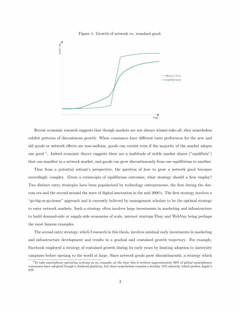
Figure 1: Growth of network vs. standard good.

Recent economic research suggests that though markets are not always winner-take-all, they nonetheless

exhibit patterns of discontinous growth. When consumers have different taste preferences for the new and

old goods or network effects are non-uniform, goods can coexist even if the majority of the market adopts

one good 1. Indeed economic theory suggests there are a multitude of stable market shares (”equilibria”)

that can manifest in a network market, and goods can grow discontinuously from one equilibrium to another.

Thus from a potential entrant’s perspective, the question of how to grow a network good becomes

exceedingly complex. Given a cornucopia of equilibrium outcomes, what strategy should a firm employ?

Two distinct entry strategies have been popularized by technology entrepreneurs, the first during the dot-

com era and the second around the wave of digital innovation in the mid 2000’s. The first strategy involves a

“go-big-or-go-home” approach and is currently believed by management scholars to be the optimal strategy

to enter network markets. Such a strategy often involves large investments in marketing and infrastructure

to build demand-side or supply-side economies of scale, internet startups Ebay and WebVan being perhaps

the most famous examples.

The second entry strategy, which I research in this thesis, involves minimal early investments in marketing

and infrastructure development and results in a gradual and contained growth trajectory. For example,

Facebook employed a strategy of contained growth during its early years by limiting adoption to university

campuses before opening to the world at large. Since network goods grow discontinuously, a strategy which

1To take smartphone operating systems as an example; at the time this is written approximately 80% of global smartphonesconsumers have adopted Google’s Android platform, but there nonetheless remains a healthy 15% minority which prefers Apple’siOS

3

purposefully contains this snowball effect is counterintuitive and seems unlikely to succeed. My thesis shows

that such a strategy can nonetheless be successful given certain features of a network market and good. For

ease of reference, I shall refer to the second entry strategy as “lean” entry throughout my thesis, and the

resulting growth trajectory as “diffusion,” as opposed to tipping.

2.3 Research Scope

Some definitions are in order before proceeding. First, we must define growth. The concept of firm growth

in management scholarship dates back to Penrose’s theory of the firm (1959) and Schumpeter’s theory

of “creative destruction” (1961). My thesis does not aim to make predictions about growth of a firm or

industry, a far more complex and ambitious topic than the growth of a single good. Moreover, I often take

the perspective of the entrepreneur producing a single good, for which firm and good growth are inextricably

linked.

To measure a network good’s growth, one might track a number of performance variables, including

adopter growth, product growth, revenue growth, and profit growth. While I focus primarily on adopter

growth, the metric for growth is formally defined when presented in context.

Regardless of how growth is measured, for a good to grow, a firm must first enter a market, attract an

increasing number of adopters over time, and prevent incumbents or new entrants from eroding its market

share. Thus any theory of entry and growth must answer the following 3 questions, addressed in the scope

of this thesis:

1. How can a producer of a network good successfully enter the market?

2. How can a producer of network good attract an increasing number of adopters over time?

3. How can a producer of a network good sustain adoption and/or erect barriers against incumbents and

new entrants?

A fourth and final question, outside the scope of my thesis but equally important for growth, is how

a producer of a network good can grow the total size of the market. As we shall see in context, growing

the total size of a network market does not necessarily invite entry 2. In network markets, the dynamics of

market and industry growth may disproportionately benefit incumbent goods, thus placing further urgency

on questions 1-3.

2In contrast with markets studied in the classic empirical industrial organization literature such as Bresnahan and Reiss(1991) who find that towns with larger populations invite more entry of service providers such as doctors, dentists, druggists,plumbers, and tire dealers.

4

To answer the questions above, I present a set of three self-contained research papers whose methodologies

and results mutually inform each other. The first paper proposes a novel theoretical framework to explain the

puzzle of disparate patterns of entry in network markets. The second and third paper presents contrasting

empirical contexts of two network goods: one a financial innovation, and the other a digital innovation.

Finally, the conclusion interprets the empirical results of papers two and three in the context of both classic

and novel theories of network goods. The first paper appears in chapter 4, the second in chapter 5, and the

third in chapter 6. The conclusion appears in chapter 7. I begin my exposition with a brief overview of the

existing literature on network goods in chapter 3.

3 Classic Theories of Network Goods

The industrial organization and strategic management literatures have established several stylized facts of

network markets. First is that network effects cause consumers to play a coordination game when making

adoption decisions: for a new network good to successfully enter the market, some consumers must adopt it

simultaneously (coordinate). Second, when there are switching costs, such as technology lock-in, search costs,

or transaction costs, this need for coordination creates barriers-to-entry which makes entry for newcomers

very difficult. Third, network goods tend to have discontinuous growth trajectories marked by rapid success

or failure (“tipping”), rather than the diffusion s-curve typical of many other innovations. I now explain in

further depth our current state of knowledge and the intellectual gaps my thesis attempts to fill.

3.1 Network Effects and Coordination

Classic theories of network effects show that consumers coordinate on the adoption of a single, or few

dominant network goods. In the simplest model of a network market proposed by Farrell and Saloner

(1986) [15], adoption consists of a game where a consumer in the market can adopt either an old or a new

network good (for example, an old versus a new technology). Since a good becomes more valuable as its

adoption increases, rational consumers necessarily coordinate either on the old good, an outcome which the

authors call consumer inertia, or coordinate on the new good, which the authors call consumer momentum.

For example, consider the following static game with two players, illustrated in normal form. Since

coordination yields an additional α units of utility over a good’s intrinsic value of x, the game’s equilibria

consist of “adopt good A,” “adopt good B,” or mix between A and B with 50% probability. Only the first

two equilibria are stable. One can easily generalize this game to one with n players, yielding stable equilibria

5

“all consumers adopt good A” and “all consumers adopt good B.” The dual nature of equilibria reflects the

“winner-take-all” phenomenon, where consumers eventually converge on a single dominant good, despite the

fact that its competitor may have equal or even greater intrinsic value [28] [29].

Example 3.1.

More recent economic theory shows that many network markets are not winner-take-all. If consumers

have differing preferences, that is some consumers have intrinsic utility y < x for good A while others

have y > x, then goods A and B can coexist and there are multiple equilibria market shares. However,

coordination still occurs. Indeed, in the revised game below, all consumers with higher preference for good

A will coordinate on good A, and all consumers with higher preference for good B will coordinate on good

B, as long as the fraction of consumers who prefer A versus B are approximately equal (precisely, between

12 −

y−x2α and 1

2 + y−x2α ).

Example 3.2.

These examples illustrate that consumer coordination is a fundamental feature of network markets. The

outcome of competition may not be winner-take-all; but, as we shall see below, market shares usually favor

the incumbent. This is due to switching costs, which a consumer incurs when switching from a good they

have already adopted to a new good.

6

3.2 Barriers-to-Entry in Network Markets

Though consumers are unbiased toward the new or old good in a frictionless market, they tend to coordinate

on incumbent goods when it is costly to switch to new goods. In other words, coordination acts as a barrier-

to-entry in the presence of switching costs [16]. To understand this, consider that in the first game above,

any positive cost γ > 0 of adopting good B, corresponding to payoffs (x + α − γ, x + α − γ), will render

“adopt good A” a unique equilibrium.

Switching costs tend to be common in network markets, especially when there is learning or search

associated with adopting new goods. They may lead to a net utility loss for consumers despite the utility

gain from network effects, if a dominant good is inferior to barred entrants. For example, I show in section

5 that startup exchange-traded products generally fail to gain traction in markets with incumbent ETPs,

despite offering lower prices (expense ratios) and identical quality (fund composition).

The strategic management literature has suggested several “go-big-or-go-home” strategies to overcome

these barriers-to-entry. Examples include preannouncing a product before it is released [30], using penetration

pricing [48] [19], bundling with existing goods [13], or investing in product quality [49]. All involve building

early demand-side economies of scale from actual or expected adopters. As a consequence, they tend to be

capital-intensive, and are not always feasible or profitable in practice.

3.3 Growth of Network Goods

Classic theories of network effects show that adoption of network goods grows discontinuously rather than

follows a standard diffusion s-curve [10]. However, discontinuous growth, or tipping as it is sometimes called,

generally will not occur if early adoption falls below a critical mass [14]. This has lent additional support

for the large-scale entry strategies described above.

Only recently have scholars pointed out that models from the classic theory rely on a crucial assumption:

that externalities have homogeneous or “global” network structure. Examples of homogeneous network

structure include, in the language of graph theory, a “complete” network where every consumer (node) is

linked to every other consumer (node), and a bipartite network containing two sets of consumers, with edges

distributed evenly between the two sets3.

3In this thesis I consider only bipartite networks where every node on one side is linked to every node on the other side.

7

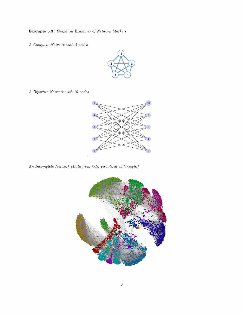
Example 3.3. Graphical Examples of Network Markets

A Complete Network with 5 nodes

A Bipartite Network with 10 nodes

An Incomplete Network (Data from [34], visualized with Gephi)

8

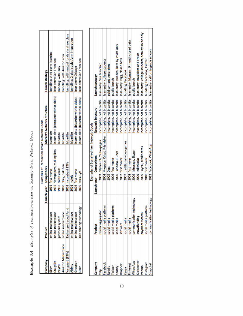
The assumption of homogeneous network structure has remained unchallenged in part because it accu-

rately reflects the nature of many network goods. For example, externalities generated by transaction-driven

goods such as market exchanges are approximately similar to the structure of a bipartite network. A key

feature of transaction-driven network goods is the anonymous nature of consumer interactions; this is what

creates structural homogeneity in the distribution of links between consumers.

In contrast, interactions for socially-driven network goods are not anonymous. For example, consumers

using a social media platform benefit from adoption of only a subset of other consumers, i.e. their friends. In

this case externalities have network structure which is “incomplete” or “local”: containing communities of

consumers, varying node degrees (number of links), and other heterogeneous structural features. The figure

in Example 3.3 depicts an actual friendship network from social media platform Facebook.

Example 3.4 illustrates case studies of successful transaction-driven versus socially-driven network goods

and their respective entry (launch) strategies. While purely anecdotal, it is nonetheless interesting to note

that entry strategies differ widely between transaction-driven and socially-driven network goods. In particu-

lar, “lean” entry strategies where companies purposefully restricted early adoption to a subset of consumers

appear more frequently in the list of socially-driven network goods. Among examples of transaction-driven

network goods, the only companies which restricted early adoption were Craigslist, Groupon, and Uber,

which all serve markets with incomplete network structure due to concentration of externalities within cities.

9

Exam

ple

3.4

.E

xam

ple

so

fT

ran

sact

ion

-dri

ven

vs.

Soc

iall

y-d

rive

nN

etw

ork

Goo

ds

10

More recent economic literature has explored properties of markets with incomplete network structure, or

“local” network effects [44] [8] [33], but our understanding of entry and growth in these markets is still in its

infancy. In particular, there has been little research on how firms can tailor their entry and growth strategies

to appeal to structural features of the market. In contrast, a rich Marketing literature studies how firms can

encourage the growth of viral goods by targeting adoption of subsets of consumers (“seeding”) [20] [4].

An important result emerging from the marketing literature is that it is optimal for firms to seed con-

sumers central to the network [7] [23] [5]. It has an appealing intuition since well-connected consumers,

such as those with more links to others in the network, allows a viral good to reach a wider audience.

Unfortunately, strategies for the growth of viral goods do not directly extend to network goods.

Their mechanism of growth differs in at least two ways. First, viral goods grow through probabilistic

transfer rather than consumer coordination. Therefore their method of transfer is closer to that of an

epidemiology model than a network effects model. Second, once a viral good is transferred there is no effect

on other adopters if the adopter who transferred the good stops adopting; therefore stability of adoption is

generally not a concern. Not so with network goods: an equilibrium adoption level in a network market can

easily be reversed if some adopters stop adopting.

To summarize, the current state of our knowledge is that network markets contain barriers-to-entry,

the growth of network goods follows a discontinuous trajectory, and that these phenomena are driven by

fundamental features of the market (i.e. consumer coordination) rather than firm actions. We have limited

knowledge about entry in markets with arbitrary network structure, the process by which discontinuous

growth occurs in general network markets, and their implications for firm strategy. These are the intellectual

gaps my thesis seeks to fill.

11

4 Lean Entry in Network Markets

4.1 Introduction

This paper examines the entry and growth strategy of a firm producing a single good with network effects.

The firm’s profit rests on the adoption of this good, which is produced with zero marginal cost but is costly

to launch. An example of such a firm would be a start-up company producing a digital product with network

effects.

Conventional wisdom from researchers and industry experts suggest that consumer coordination and

switching costs in network markets create barriers-to-entry favoring incumbent goods. The claim is that

when is costly to switch to a new good, all consumers will coordinate on the old good due to network effects.

The ”10x” rule of thumb espoused by Andy Grove of Intel offers a sense of magnitude for the difficulty of

entry: new technologies must be ten times better than old technologies to succeed. Case studies of persistent

incumbent network goods include technology standards such as the QWERTY keyboard, software platforms

such as Microsoft Windows, and market exchanges such as Ebay.

This paper shows that contrary to conventional wisdom, network effects do not create barriers-to-entry in

all network markets and can even facilitate entry in some network markets. In markets where network effects

are structurally homogeneous, as depicted in classical theories of network effects, entry is indeed difficult.

However, this paper shows that the strength of barriers-to-entry in network markets is determined by a

structural metric related to network cohesion. Firms can seed subsets of consumers with cohesive network

structure, including “boundary spanners” within these subsets, to grow adoption discontinuously.

The motivating example for this paper is Facebook’s entry in the market for social communication

technology. Social communication technologies are a particularly apt example of a market where the structure

of network effects is incomplete. Facebook started up its adoption by appealing to a small cohesive group

of early adopters: students at elite universities. Few believed it could enter the industry through a niche

market and “gradually through [a] carefully calculated war against all social networks, become the one social

network to rule them all” [1]. The main goal of this paper is to show, through a formal model, a plausible

mechanism for this counterintuitive outcome.

To do this, we introduce a formal model of the growth of a network good in a network market with

arbitrary network structure. Growth occurs as a dynamic graphical game between consumers, who myopi-

cally best respond to the adoption of their peers. The firm can endogenously affect growth of its good by

seeding early adopters. We show that barriers-to-entry can be an order of magnitude weaker in markets

12

with heterogeneous (“incomplete”) network structure than in markets with complete or bipartite network

structure. We also derive a set of three strategic implications using this model: 1) lean entry strategies are

especially useful when start up costs are high 2) a firm should strive to be a first mover whenever possible,

and 3) a firm can predict its likelihood of success using information about network structure.

The formal model of discontinuous growth in this paper is similar to the approach taken by Morris

(2000) [36], who uses a graphical game of binary choice to show conditions under which the behavior of a

seeded set of players on an arbitrary network can spread to the population at large. It verifies the intuition

first introduced by Rohlfs (1974), who suggested that firms can exploit heterogeneity in network structure

to lower the cost of entry. To the best of the author’s knowledge, no prior work has formalized Rohlf’s

insightful observation, explored its strategic implications, or tested its validity on real-world network data.

4.2 Model

4.2.1 Consumers

Let there be a network of consumers linked by a set of undirected interactions. Consumers may interact

socially, via economic transactions, or shared use of a technology. Interactions between consumers generate

direct positive externalities. For example, consumers of a social communications technology benefit from the

participation of other consumers with whom they interact.

Let nodes N = {1, . . . , n} represent the set of consumers and links L = {lij |i, j ∈ N} represent their

interactions, where lij exists if and only if i and j interact and lij = ∅ otherwise. Call consumers with whom

i ∈ N interacts the peers of i, denoted L(i) = {j ∈ N s.t. ∃ lij ∈ L}. Consumers and interactions form a

network, given by graph G(N,L). A network G(N,L) is complete if L(i) = N\{i} for all i ∈ N and empty

if consumers do not interact, that is L = ∅. A network is incomplete if it is neither empty nor complete.

Example 4.1. Example of a complete network where L(i) = N\{i} for all i ∈ N .

Suppose each consumer i ∈ N can choose one of two options: to adopt or not adopt an entrant firm’s

13

network good, denoted by xi = 1 and xi = 0 respectively. Let consumers’ choices be captured by state

x = (x1, . . . , xn),

where x ∈ X = {0, 1}n, and let ||x|| denote the number of adopters in this state, or ||x|| =∑i∈N xi.

Consumers hold intrinsic value θ for the good, and externality value α for each peer adopting the good.

I assume for clarity that all consumers value the focal good equally and benefit equally from their peers.

Suppose further that consumers hold values v = (v1, . . . , vn) for their outside option. Consumer i’s payoff is

captured by a utility function Uγi(·) with parameters γ = (θ, α, v):

Uγi(x) = θ + α∑j∈L(i)

xj if xi = 1,

Uγi(x) = vi otherwise.

Letting Uγ denote the vector of utility functions (Uγ1, . . . , Uγn), define a network market as a nonempty

network of consumers and vector of utility functions {G,Uγ}.

I assume a consumer does not adopt a network good unless he or she strictly prefers it over their outside

option. Thus from the utility functions above, a rational consumer adopts if and only if the number of his

or her adopting peers exceeds a certain threshold, or∑j∈L(i) xj >

vi−θα . Call this threshold

ti =vi − θα

. (1)

and let t be the vector of consumers’ thresholds. Note ti depends on the value of a consumer’s outside option

and thus may differ for each i ∈ N .

The setup above describes a graphical game where agents are consumers, actions are adoption or non-

adoption, and payoffs are utilities from the entrant’s network good and the outside option respectively. A

consumer’s best response is to adopt if and only if the number of his or her adopting peers exceeds its

threshold: b(·) = (b1(·), . . . , bn(·)) such that bi(x) = 1 if∑j∈L(i) xj > ti, and bi(x) = 0 otherwise. We can

characterize the outcome of diffusion x∗ as a pure strategy Nash equilibrium where each consumer plays a

best response to the adoption of their peers:

bi(x∗) = x∗i ∀ i ∈ N. (2)

14

Since multiple states may satisfy condition (2), call the set of equilibria X∗. Here let us make an important

observation: any game in a network with complete network structure such as example 4.1 supports only two

equilibrium states: “all adopt” and “none adopt,” but incomplete networks (networks which are neither

empty nor complete) may support many equilibrium states with partial levels of adoption. Thus in general,

the number of equilibria in X∗ may be quite large. The example below illustrates this observation (for

simplicity assume thresholds are ti = 1 for all i ∈ N).

Example 4.2. Multiple equilibria in a market with incomplete network structure.

This multiplicity of equilibria in incomplete network markets allows only part of the market to adopt

the entrant’s good in equilibrium, and outcomes are not binary as they are in complete networks. When

the market shifts from one equilibrium to another, it undergoes a process whereby demand either grows or

wanes discontinuously. Call this the diffusion process (DP).

Suppose consumers react in a sequence of states {xτ}∞τ=1 to an initial state x1 = x. Call this sequence

locally rational if and only if at each iteration τ > 1, either xτ+1i = xτi or xτ+1

i = bi(xτ ) for all i ∈ N . That

is, the sequence of behavior is locally rational if and only if at each iteration, consumers either do nothing

or they best respond to the previous state of adoption.

Starting from an initial state x, let the diffusion process (DP) be defined as follows: first all consumers

i ∈ N whose best response is 0 switch their actions to 0, and this subtractive process repeats until no further

consumers wish to switch to 0. Then, all consumers i ∈ N whose best response is 1 switch their actions to

1, and this additive process repeats until no further consumers wish to switch to 1. It is easy to show that

DP is locally rational and is guaranteed to reach an equilibrium.

More importantly, DP reaches the lowest equilibrium reachable by a locally rational dynamic process in

the following sense: say that DP reaches an equilibrium φ(x) ∈ X∗ from state x if it stops at some iteration

τ = T <∞. Call state y ∈ {0, 1}n weakly lower than y′, denoted y � y′, if and only if yi ≤ y′i for all i ∈ N .

A similar ordering holds for states with weakly (�) greater adoption. Proposition 8.1 in the appendix shows

if φ′(x) is the outcome of any other locally rational dynamic process, then φ(x) � φ′(x). This feature of DP

15

is nontrivial and allows us make the most conservative predictions about demand for the entrant’s good.

DP has the intuitive property that weakly greater initial states reach weakly higher equilibria, a property

I formalize in Proposition 4.1 below. However, the outcome of DP depends not on the mere number of early

adopters, but on their structural identity. States with greater numbers of early adopters do not necessarily

reach higher levels of demand. Example 4.3 shows DP in the same network from initial states x and x′, both

which contain four early adopters, but the first reaches an equilibrium which is lower than the second (again

let thresholds ti = 1 for all i ∈ N).

Proposition 4.1. Demand D(x) = ||φ(x)|| is weakly increasing in greater initial states of adoption: for

x � x′, it holds that D(x) ≥ D(x′). However, D(x) ≥ D(x′) does not imply x � x′ or ||x|| ≥ ||x′||.

Example 4.3. Diffusion from two different states in a market with incomplete network structure.

4.2.2 Firm

Let there be an entrant firm capable of producing a single network good at zero marginal cost to serve

the network market described above. Its action space consists of three decisions, made sequentially: enter

if profit is positive, start up demand by “seeding” a state of early adoption, and charge a static price to

consumers. An example of such a firm would be a start-up aiming to displace an incumbent technology. I

assume the firm does not face competitive response is thus optimizes profit as a monopolist for the duration

of the model.

16

The firm’s good is characterized by two parameters: θ indicating intrinsic quality relative to quality of

the outside option, and α indicating the strength of adoption externalities. Unless otherwise specified, I

assume these parameters are exogenous.

To start up demand for its good, the firm seeds a state of early adoption x, from which DP reaches D(x).

For example, the firm may seed through beta testing, marketing, or targeted discounts. Assume the firm

seeds only once: the firm cannot seed adoption in periods 1 < τ ≤ T due to the speed of diffusion. The firm

has perfect information of the market when seeding. Let the cost of seeding be given by the function c(||x||)

where ||x|| is the number of early adopters. Assume costs increase monotonically in ||x|| and exceed zero

when ||x|| > 0.

The market undergoes a diffusion process (DP) immediately after seeding. Define growth to be the

difference between the number of early adopters ||x|| and equilibrium demand D(x) reached by DP. Assume

the firm charges zero price to consumers before and during DP. After the market reaches equilibrium, the

firm charges a price pi to consumer i ∈ N equal to i’s willingness-to-pay (WTP). For example, in a complete

network market, all adopters have the same value for the firm’s good in equilibrium, given by θ + α(n− 1);

the firm charges price θ+α(n−1)−ε such that adoption continues to be incentive compatible in equilibrium.

Henceforth I omit ε for notational clarity.

The firm’s profit function is

π(x) =∑i∈N

φi(x)pi − c(||x||), (3)

where φi(x) is i’s equilibrium state of adoption, pi = θ+α∑j∈L(i) xj , and c(||x||) is the firm’s seeding cost.

4.2.3 Assumptions

The model above makes three major assumptions. First, it assumes that competitors do not respond strate-

gically to the entrant’s actions. Second, it assumes consumer choice is binary and that consumers are myopic

when making decisions. Third, it assumes firms have perfect information of network structure. I will now

discuss conditions under which these assumptions are likely to hold.

Assumption 1: Incumbent Inertia

The model above assumes that the firm producing the incumbent network good does not respond strate-

gically to actions of the entrant firm. In particular, it assumes the incumbent firm does not “counterseed” in

response to the entrant’s actions. This assumption is a simplification made for model tractability and would

likely be invalid in a highly competitive environment where firms frequently update their information and

17

have the ability to act with great speed. For example, the model would likely be a poor fit for a context in

which incumbent firms collect data on customer networks and carefully monitor competitor growth. In fact,

any counterseeding by the incumbent, even if it is untargeted, will make the entrant good’s growth more

difficult than what the model dictates.

However, several case studies in the brief history of network goods have shown that incumbents in

established industries often do not respond strategically or respond too slowly to the entry of “disruptive”

technologies. Examples include film producers’ response to digital camera technology, video rental companies’

response to online streaming video, print newspapers’ response to online classifieds, MySpace’s response to

Facebook, and more recently, taxi companies’ response to ride-sharing applications.

Though examining reasons why this occurs is outside the scope of this thesis, there are several reasons

why it might hold in practice. One is that incumbents do not perceive entrants to be a threat due to

their low early market share. Another reason, captured by the theory of Disruptive Innovation, is that

incumbents cannot predict future changes in consumer tastes and technological quality. My model offers two

additional explanations for lack of incumbent response: the fact that growth of the entrant good can stagnate

at low equilibria (hiding its ultimate potential to quickly grow to greater equilibria), and the difficulty of

counterseeding in a complex environment.

To flesh out the first explanation, my model shows that a market with arbitrary (incomplete) network

structure generally supports several demand equilibria, each of which can seem like a point of diminishing

growth for the entrant good from the perspective of an unsuspecting incumbent. However, small pertur-

bations to adoption can easily cause demand to grow to a greater equilibrium, or diminish to a lower

equilibrium. Therefore, while an entrant good may appear to stop growing for a time, it may simply be

reaching an intermediate equilibrium which belies its ultimate potential for growth.

As for difficulty of counterseeding, the model does not assume that firms know exactly which subsets of

consumers to seed, even with perfect information of network structure. This is because finding a globally

optimal seed set in an arbitrary network market is NP-hard. The purpose of my model is to show what

could happen if the entrant, perhaps by luck, seeds a favorable group of consumers which then sets off rapid

growth. The entrant’s outcome may not be deterministically replicable by either the entrant or incumbent.

Assumption 2: Binary Consumer Choice

The second major assumption of the model is that a consumer can adopt only one of two goods, when

in reality he or she could have multiple goods to choose from, and adopt more than one at the same time.

Again this assumption is made for model tractability. This assumption is more likely to hold in a world

18

where the choice set is small and consumer attention is limited. If there are multiple goods to choose from

and consumer choice is closer to random, the model would not be appropriate for predicting competitive

outcomes. Similarly,the assumption of consumer myopia reflects decision-making in a world with sufficient

complexity. If the world is so simple that consumers can predict the future and game firms’ entry decisions,

then alternative models, such as ones where consumers have rational expectations of future market shares,

would likely offer more accurate predictions of market outcomes.

One potential justification for this assumption is that, barring cooperation between firms, the size of

the choice set does not affect the model’s results. For example, a model allowing consumers to adopt more

than one good at a time, or “multi-homing” in the two-sided platforms literature, can be reduced to a

threshold model by mapping a continuous action space representing consumption allocation to a binary

action space representing whether a good receives the largest share of consumption. Similarly, a model

allowing consumers to choose one of multiple goods could be generalized to the threshold model in equation

1 as long as a consumer compares the entrant’s good to the best of her outside options.

Assumption 3: Perfect Information

Finally, the model assumes the entrant firm has perfect information of network structure. I make this

assumption because the lower cost of data storage and analysis is increasingly allowing firms to have near

perfect information of markets and consumers. For example, companies often collect competitor and con-

sumer data in order to make strategic decisions. Due to advanced data collection techniques, an entrant

could feasibly know detailed features of an entire market, including its network structure. Moreover, having

perfect information of network structure does not imply a firm can seed optimally. In other words, an entrant

can use data on network structure to improve but not optimize their entry and seeding decisions, which I

later demonstrate using a simulation.

Where this assumption is likely to be invalid is if the incumbent purposefully obfuscates or distorts

information as a way to fool the entrant, via signaling or other means. Since observing growth of the

incumbent’s good yields information about network structure to the entrant, this “information” can be

strategically manipulated. In addition, firms may have asymmetric information due to differing abilities to

collect data about each other. Such a model, while potentially insightful, is outside the scope of this thesis.

4.3 Relationship Between Network Structure and Growth

So far we have characterized diffusion as a sequence of consumer best responses to the adoption of their peers.

I now show that the path of diffusion has a one-to-one correspondence to a metric of network structure which

19

I call t-cohesion, where t is the vector of consumer thresholds. By characterizing DP as a function of network

structure, we can derive insights about how the network structure affects entry and growth.

Recall consumer i’s best response is to adopt a network good if and only if its number of adopting peers

exceeds its threshold ti = vi−θα . Assume henceforth that consumers’ outside option is an incumbent network

good. In this case, vi is a function of i’s number of nonadopting peers. Normalizing θ to be the intrinsic

value of the entrant’s good relative to the outside option, we get vi = α(di−∑j∈L(i) xj), where di is i’s total

number of peers or degree. Thus, i’s best response to adopt if and only if

∑j∈L(i)

xj >di2− θ

2α. (4)

Note that when θ = 0, the expression above simply states a consumer needs more than half their peers to

adopt the entrant good before they switch from the incumbent good to the entrant good.

This leads us to define network cohesion and its relationship to diffusion. Consider a set of consumers

A ⊂ N . A priori, each consumer i ∈ A has a proportion pi of its peers within A and the rest outside of

A. For example, a consumer in A which has two peers within A and three outside of A has pi = 25 . The

proportion of a consumer i’s peers within A can be denoted pi = |L(i)∩A|di

, where | · | is set cardinality. Define

A’s cohesion to be the value of the smallest pi of a consumer in A. The example below shows a set of

consumers whose cohesion is 12 .

Example 4.4. A weakly 12 -cohesive set of consumers

Network cohesion describes the proportion of interactions consumers have with other consumers in a

set versus with the network at large. For example, a community of consumers segregated by age, religion,

or political preference may be highly cohesive, choosing to interact primarily with one another. Loosely

speaking, the more cohesive a set of consumers, the greater fraction of externalities exist within themselves

versus between themselves and others.

Taking a slight modification of the definition above, call A strictly (weakly) t-cohesive if pi is greater

than (at least) tidi

for every i ∈ A. A set of consumers would fail to be strictly t-cohesive if some i ∈ A does

20

not have enough peers in A, i.e. |L(i)∩A| ≤ ti. Note that when θ = 0, thresholds are ti = di2 and t-cohesion

reduces simply to 12 -cohesion.

Our first result relating diffusion to network structure is that a state x is self-sustaining if and only if

its adopters are strictly t-cohesive. A state is self-sustaining if adopters in the state continue adopting even

if no additional consumers adopt during the diffusion process. In contrast, if a state is not self-sustaining,

early adopters may stop adopting before their peers have a chance to best respond and early adoption will

not be stable.

Let A(x) be the set of adopters in a state x, and say that x is self-sustaining if it is a best response for

all i ∈ A(x) to adopt given that all other consumers j ∈ A(x) adopt. We can relate sustainability of early

adoption to network structure by the following proposition:

Proposition 4.2. State x is self-sustaining if and only if A(x) is strictly t-cohesive.

Our second result relates to the outcome of diffusion: what demand can the firm expect in equilibrium?

The answer again depends on t-cohesion. Proposition 4.3 below shows that adopters at every period of

diffusion form a strictly t-cohesive set which is nested within the set of adopters in the subsequent period of

diffusion. Networks which facilitate diffusion contain a sequence of nested and successively larger t-cohesive

sets of consumers which gradually decrease in the proportion of their interactions with the rest of the network.

This structure allows adoption to diffuse from a central t-cohesive set and proceed outwards, like a sequence

of nested Matryoshka dolls.

Proposition 4.3. Assume x is self-sustaining. At every iteration τ ∈ {1, 2, . . . , T}, the diffusion process

reaches a strictly t-cohesive set A(xτ ) such that A(x) ⊂ A(xτ−1) ⊂ A(xτ ) ⊂ A(xT ).

Diffusion also stops at the boundary of a strictly t-cohesive set of nonadopters, if one exists. Let C =

N\A(xT ) be the set of nonadopters in equilibrium. The following corollary states that diffusion stops when

nonadopters are too cohesive among themselves.

Corollary 1 (4.3). Let d be the vector of consumers’ degrees in the network. When the outside option is a

network good, diffusion stops at iteration τ = T where the complement of A(xT ), C = N\A(xT ), is weakly

(d− t)-cohesive.

Propositions 4.2, 4.3, and 1 show that network cohesion is a double-edged sword for growth of a network

good. On the one hand, cohesion of early adopters is necessary because otherwise early adoption is not

sustainable and leads to zero demand growth. On the other hand, when early adopters are too cohesive,

21

adoption cannot diffuse widely. In addition, when nonadopters in some period of diffusion are too cohesive,

diffusion stops and adoption of the entrant’s good will be fragmented.

For example, it may be easier to convince a community of consumers of the same age, religion, or political

preference to sustain early adoption of a good due to externalities within themselves, but it is simultaneously

difficult to exploit subsequent demand growth due to the lack of externalities between themselves and others.

Similarly, a cohesive community of nonadopters may never adopt a mainstream network good because they

value an alternative good highly within themselves.

This brings us to the result that consumers which stimulate demand growth have an almost equal number

of nonadopting peers as adopting peers in some period of DP. I borrow terminology from the sociology

literature and loosely interpret these consumers as “boundary spanners” [2], in reference to individuals with

dispersed ties to multiple groups of agents in a network.

Formally, call consumer i a boundary spanner if |L(i)∩A(xτ−1)| = btic+1 and |L(i)∩A(xτ+1)| = dtie−1

where i adopts in period τ ∈ {1, 2, . . . , T}. Boundary spanners allow the firm to balance the sustainability

properties of proposition 4.2 with the diffusive properties of proposition 4.3 when seeding. Contrary to

the Marketing literature on viral diffusion, these critical consumers are neither the most “central” to the

network, nor “brokers” who link otherwise disconnected parts of the network.

Networks Optimal For Growth

To make asymptotic predictions about seeding and demand growth needed for our main results about

lean entry, we must derive some sort of demand function predicting the bounds of diffusion from a fixed

number of early adopters ||x||. Networks which are optimal for demand growth, in the sense that DP

reaches the highest possible equilibrium demand from ||x|| early adopters, have nested t-cohesive network

structure and maximize the number of links between successive t-cohesive sets. In particular, optimally

diffusive networks contain as many boundary spanners as possible given reasonable assumptions about their

frequency of occurrence in the network.

Recall that nested t-cohesive networks contain a sequence of nested and successively larger t-cohesive sets

of consumers which gradually decrease in the proportion of their interactions with the rest of the network.

Formally, a network has nested t-cohesive structure if there exists a sequence {Ak}Tk=1 of t-cohesive sets in

the network such that A1 = A(x), Ak−1 ( Ak, and |L(i) ∩Ak−1| ≥ btic+ 1 for all i ∈ Ak\Ak−1.

For a nested t-cohesive network to be optimal for demand growth, it must have the additional property

that |L(i) ∩ Ak−1| = btic + 1 for some consumers i ∈ Ak\Ak−1. Assume there are a fraction γ of such

boundary spanners in the network. The intuition is as follows: given a finite number of early adopters, there

22

are a finite number of “incoming” links between early adopters themselves. To satisfy t-cohesion, the number

of incoming links limits the number of “outgoing” links from the early adopters to other consumers in the

market. The optimally diffusive network simply maximizes the number of outgoing links in each period of

diffusion while preserving t-cohesion, assuming the fraction of boundary spanners satisfies γ < αθ .

Proposition 4.4 shows that demand has a closed form D̄(x) = ||x||(||x|| − 1) + θαγn in an optimally

diffusive network, where γ is the fraction of boundary spanners. For the remainder of the analysis below,

assume the fraction of boundary spanners satisfies γ < αθ , such that θ

αγ < 1.

Proposition 4.4. Demand from seeding state x is weakly bounded above by D̄(x) = ||x||(||x||−1) + θαγn for

any market of size n with arbitrary network structure, where γ is the fraction of boundary spanners during

diffusion.

In the special case when θ = 0, every consumer i in an optimally diffusive network has exactly bdi/2c+ 1

peers adopting immediately prior to i’s adoption; that is, every consumer is a boundary spanner during

diffusion. Demand reaches the upper bound D̄(x) = ||x||(||x|| − 1) from ||x|| early adopters, assuming x

is t-cohesive and nested in the center of a sequence of larger t-cohesive sets. By construction, the network

supports only two equilibria, “all adopt” and “none adopt.” The example below illustrates this corollary of

Proposition 4.4.

Corollary 2 (4.4). In the special case when θ = 0, the class of optimally diffusive networks have nested

t-cohesive structure and for each Ak ∈ {A1, A2, . . . , N}, all i ∈ Ak\Ak−1 have bdi/2c+ 1 peers in Ak−1 and

ddi/2e − 1 peers in Ak+1.

Example 4.5. An optimally diffusive network when θ = 0 and A(x) = {1, 2, 3, 4, 5}.

Proposition 4.4 yields a class of networks which describes the “best-case” network given a “worst-case”

diffusion process: DP predicts a lower bound on demand in a given network, and reaches the greatest possible

demand in the class of optimal networks. Therefore, the closed form demand function above dictates the

23

minimum number of early adopters a firm must seed to ensure demand reaches a target value n in any

network market with a fraction γ of boundary spanners. Proposition 4.4 implies a firm must seed at least an

order of√n early adopters to reach full demand n as n grows large. I revisit this result in the next section.

4.4 Core Result of Lean Entry

Conventional wisdom from the network effects literature posits that a firm must make great initial investments

in scale to displace an incumbent network good. But while this wisdom holds for markets with complete and

bipartite network structure, the strength of barriers-to-entry are weaker in markets with optimally diffusive

network structure and a firm needs to seed only square root as many early adopters to enter. This is the

core result of “lean entry.”

Minimal Scale and Barriers-to-entry

Let us begin by clarifying a key assumption. Call the fewest number of early adopters a firm must seed

to earn positive profit its minimal scale needed for entry. As before, assume the firm can only seed once

and has perfect information of the market’s network structure when seeding. Define barriers-to-entry to be

an entrant’s cost of seeding its minimum scale. Assume in this section that entry is profitable if and only if

the firm seeds the lowest possible state reaching equilibrium demand n. Note the “only if” part acts as an

intentionally conservative assumption. The “if” part requires seeding costs not to grow too quickly in the

number of early adopters, an assumption which is relaxed in the next section.

Core Result of Lean Entry

When the market has complete or bipartite network structure, a firm’s minimal scale grows linearly with

size of the market n. Barriers-to-entry are consequently strong. As a rule of thumb, the firm must seed more

than half the market to enter. This follows directly from the observation that a firm must seed a t-cohesive

set for adoption to be self-sustaining, but the smallest t-cohesive set in these markets contain more than half

the total number of consumers.

Recall the expression for thresholds when the outside option is a network good: ti = di2 −

θ2α . Since di =

n−1 for all n consumers in a complete network, it is easy to verify that sets of fewer than b(n−1)/2− θ2αc+2

consumers are not t-cohesive in a complete network because every consumer in this set would have fewer

peers in the set than her threshold. Thus when θ = 0, the firm’s minimal scale in a complete network is

b(n− 1)/2c+ 2. This result generalizes to arbitrary θ as long as θ is independent of n. A similar result holds

for bipartite networks.

24

Lemma 4.1. The minimal scale required to enter a complete or bipartite network market of size n grows in

the order of O(n) as n→∞.

Barriers-to-entry in optimally diffusive networks, on the other hand, are considerably weaker: the firm’s

minimal scale grows at most with the square root of n. This result follows from Proposition 4.4 which states

that diffusion from state x reaches demand D(x) = ||x||(||x|| − 1) + θαγn in an optimally diffusive network.

Setting demand to n, we see the firm can seed a state with O(√n) early adopters to reach positive demand.

Lemma 4.2. The minimal scale required to enter an optimally diffusive network market of size n grows at

most in the order of O(√n) as n→∞.

The minimal scale needed to enter an optimally diffusive network market of size n therefore reaches

at most the square root of the minimal scale needed to enter a complete network market of size n as

n→∞. Since this relationship is independent of the seeding cost function, it follows that barriers-to-entry

in a complete (or bipartite) network market are at least quadratically greater than barriers-to-entry in a

comparable optimally diffusive network market for any market parameters θ, α, and c(·). This is the core

result of lean entry.

Proposition 4.5. Barriers-to-entry are at least quadratically greater in a market with complete network

structure than in a comparable market with optimally diffusive network structure, irrespective of quality of

the entrant’s good and its seeding cost function.

4.5 Strategic Implications

Proposition 4.5 shows that barriers-to-entry in network markets can be far weaker in a market with incomplete

network structure than in markets described by classic theories of network goods Reference Chapter 3.. This

formally proves the intuition first laid out by Rohlfs in his 1974 paper on entry in network markets: that

sets of self-sustaining (t-cohesive) consumers can greatly reduce the cost needed to “start up” demand for

a network good. A firm choosing to enter such a market can seed these sets of consumers at a relatively

low cost and grow via diffusion (DP), a “lean” entry strategy. Specifically, a lean entry strategy entails a

sequence of actions: enter an incomplete network market, seed a self-sustaining set of adopters, and charge

a price equal to consumers’ WTP in the equilibrium attained by DP.

This section derives three insights into when and how a firm can successfully implement a lean entry

strategy. First, lean entry is a profitable strategy even when seeding costs are high, specifically when costs

grow too quickly in the number of seeded adopters to enter a complete network market profitably. There is

25

a sweet spot of seeding cost functions where a firm can and should employ a lean entry strategy. Second, the

likelihood of successful entry in an arbitrary network market can be predicted by the firm. I run simulations

using data from real-world networks to show how firms can identify markets where a lean entry strategy is

likely to be profitable. Finally, the minimum scale needed to enter a market is always lower if consumers

have not already adopted an incumbent network good, irrespective of network structure: this creates a first

mover advantage. A lean entry strategy is thus neither necessary nor optimal when firms can enter complete

network markets as a first mover.

4.5.1 When to Use Lean Entry

Recall that the firm’s action space consists of three decisions, made sequentially: enter the market if profit

is positive, start up demand by “seeding” a state of adoption, and charge consumers a price equal to their

willingness to pay. The results below indicate a firm can take this sequence of actions for an optimally

diffusive network market, seeding in the order of√n as established by Proposition 4.5, and make positive

profits. The profitability of entry depends on how quickly seeding costs grow relative to the number of seeded

adopters. The seeding cost function should also be the major strategic consideration when a firm is deciding

which market to enter, if it has a choice between entering a complete vs. optimally diffusive network market.

To obtain these results, we shall compute a range of cost functions where entering 1) an optimally diffusive

network market yields greater profit than 2) not entering and 3) entering a complete network market. Assume

market parameters and seeding costs are exogeneous and the size of the market n is large. Let us first derive

equations for optimal profit for each of the three cases as a function of n, and then compare their asymptotic

behavior when n goes to infinity.

1) Profit in an optimally diffusive network market. In an optimally diffusive network market, there are

generally multiple intermediate equilibria in addition to the equilibria “all adopt” and “none adopt”. Here

we assume the entrant firm chooses to target the equilibrium “all adopt” with demand n, and thus seeds

O(√n) early adopters. Note that when costs are sufficiently low, i.e. bounded above by c(||x||) < ||x||2(k+1),

it is optimal for the firm to target the maximal equilibrium.

To derive the profit function, assume the average degree of consumers in the optimally diffusive network

is a k-th order polynomial function of n, that is, 1n

∑i∈N di = O(nk) where 0 < k < 1. For example, the

average degree could be approximately√n. This average degree assumption places a minimum bound on

the density of adoption externalities in the market: whereas complete network markets have O(n2) links, we

26

consider an optimally diffusive network with O(nk+1) links. Lemma 4.3 proves that such a network indeed

exists.

Lemma 4.3. There exists an optimally diffusive network of size n with 1n

∑i∈N di = O(nk) where 0 < k < 1.

Suppose the firm charges a consumer’s full willingness to pay for its good in equilibrium, or pi = θ+αdi.

Under the average degree assumption, profit in an optimally diffusive network market is asymptotically

equivalent to

πL(n) = n(θ + αnk)− c(dme) where m2 −m = (1− θ

αγ)n. (5)

2) Profit from not entering. The firm earns zero profit in this case: π∗B = 0.

3) Profit in a complete network market. Since complete networks support only two equilibria, “all adopt”

and “none adopt,” it is profitable for a firm to enter a complete network market if and only if revenue

from serving the entire market exceeds the cost of seeding its minimal scale. If the firm enters, it seeds

b(n− 1)/2− θ2αc+ 2 early adopters and charges a consumer’s full willingness-to-pay (WTP) for its good, or

p = θ + α(n− 1). Optimal profits in a complete network market of size n is thus

π∗C(n) = αn2 + (θ − α)n− c(bn− 1

2− θ

2αc+ 2

). (6)

To make the exposition as clear as possible, let θ = 0 throughout the remainder of the analysis. These

results generalize fully for θ > 0, as proved in the appendix. Furthermore for notational clarity, note that

c (b(n− 1)/2 + 2) > c(n/2) and c(dme) < c(√

2n); thus it is sufficient to work with these bounds on costs of

seeding a complete and optimally diffusive network market, respectively.

I first show conditions under entering an optimally diffusive network is profitable (i.e. greater than profit

from not entering). Under the assumptions made above, optimal profits from these decisions are π∗L(n) and

0 respectively. For π∗L(n) > 0 to hold as n→∞, there must exist n0 such that

c(√

2n) < αnk+1 (7)

for all n > n0. This expression holds if seeding costs are be bounded above by a 2(k+1)-ic polynomial, where

k depends on the average degree of the network. In other words, the seeding cost function must increase

sufficiently slowly in the number of early adopters for entry to be profitable. As an example, if the average

27

degree is is√n (i.e. k = 1/2), then entry is profitable if seeding costs grow less than cubically in the number

of early adopters.

Now suppose the firm has not yet chosen which market to enter. This situation may arise in reality, for

example, when a firm has a core technology which can be “pivoted” toward one of two product-markets.

Given this context, let us establish conditions under which the firm earns greater profits by entering an

optimally diffusive network market than by entering a complete network market.

Call optimal profits in these markets π∗L(n) and π∗C(n), respectively. For π∗L(n) > π∗C(n) to hold as

n→∞, there must exist n0 such that

c(n/2)− c(√

2n) > αn2 − αnk+1 − αn (8)

for all n > n0. This expression holds if the seeding cost function increases more than quadratically in

the number of early adopters, that is, if cost grows faster than revenue from externalities in the complete

network.

Putting conditions 8 and 7 together, we see that the firm earns greatest profits by entering an optimally

diffusive network market (lean entry) if and only if the form of the cost function is bounded below by a

quadratic polynomial and bounded above by a 2(k + 1)-ic polynomial determined by the average degree

assumption. For example, when the average degree is√n, the firm earns greatest profit from lean entry

if the seeding function increases more than quadratically but less than cubically in the number of early

adopters.

Proposition 4.6. Under the average degree assumption, profits are asymptotically greater from entering an

optimally diffusive network market than from not entering the market or entering a complete network market

when the seeding cost function satisfies ||x||2 < c(||x||) < ||x||2(k+1).

To illustrate Proposition 4.6 with an example, suppose again that the average degree of the optimally

diffusive network is√n. When the seeding cost function grows slower than quadratic in scale, the firm earns

greatest profit in a complete network market, followed by the optimally diffusive network market and finally

the non-network benchmark. When the cost of seeding grows between quadratic and cubic in scale, the firm

earns greatest profit in the optimally diffusive network market, followed by the non-network benchmark, and

earns negative profit in the complete network market. Finally, when the cost of seeding grows faster than

cubic in scale, the firm earns negative profit in both the optimally diffusive or complete network market.

The table below illustrates the relationship between seeding costs and relative profits in this example.

28

Table 1: Relative profits when θ = 0 and average degree is√n

Relative Ordering

c(||x||) < ||x||2 π∗C > π∗

L > π∗B

||x||2 < c(||x||) < ||x||3 π∗L > π∗

B > π∗C

c(||x||) > ||x||3 π∗B > π∗

L > π∗C

Proposition 4.6 says there is a “sweet spot” of cost functions where lean entry is most profitable. In

general, profits depend on a balance between the value of adoption externalities and seeding costs as n grows

large. If seeding costs grow slower than adoption externalities, markets with complete network structure are

most profitable because they maximize the number of links between consumers. If seeding costs grow faster

than adoption externalities, optimally diffusive network markets are more profitable, but when costs grow

too fast, the firm is better off not entering a network market at all.

It is interesting to observe that relative profits from entering each type of market do not depend on

parameters θ and α when n grows sufficiently large. Mathematically, this is because θ and α appear only

as scalar multiples of n in the equations for price and seeding costs, so these parameters do not affect the

outcome of the asymptotic analysis. There is also an intuitive explanation for this result: whether lean entry

is a profitable strategy in large markets depends far more on seeding costs and network structure than on

the quality of the firm’s good or the strength of network effects.

Another implication of the results above is that if given a choice, a firm should enter a complete network

market unless the cost of seeding increases too sharply with respect to the number of seeded adopters. This

is because though incomplete networks are generally easier to enter, they also contain less value a firm can

potentially capture due to fewer externalities. Note however, start-up firms often cannot enter complete

network markets due to the large capital investments that must be made up front to build critical mass.

4.5.2 Lean Entry in Real-World Networks

The core result of lean entry is that barriers-to-entry are weaker in optimally diffusive networks than in

complete or bipartite networks. This claim can be generalized to an arbitrary network market. In addition,

the firm can predict the likelihood that lean entry is profitable by simulating entry and growth outcomes.

To illustrate this, I run a set of simulations on data sampled from a Facebook network, a scientific

coauthorship network, and an email network; representing a market for a social media platform, collaboration

software, and communications technology, respectively. Each trial of the simulation involved seeding a set

29

of consumers with an algorithm and running DP. The size of the seed set (scale), demand attained by DP,

and resulting profit was then recorded.

The results indicate that lean entry appears to be a viable strategy in real-world networks. Indeed, in all

the networks studied, the minimal scale needed to enter profitably was less than the scale needed to enter an

equivalent complete network (n/2). Whether lean entry is profitable depends on how well it is implemented

at the tactical level: specifically which algorithm was used to seed. I show that a simple “greedy” seeding

algorithm initialized at random consumers in the network can estimate minimal scale and barriers-to-entry

as well as predict the likelihood that lean entry will be profitable. An “optimal” seeding algorithm identifying

a highly diffusive t-cohesive subset(s) of consumers approximates the firm’s optimal profit in an arbitrary

network market. I compare these algorithms against the performance of a random seeding algorithm to show

that large-scale seeding is neither necessary nor sufficient for a firm’s success.

Data and Algorithms Description

I used network data from Stanford Large Network Dataset Collection [34] for the simulation. The first

data set is a social network with individual profiles and profiles of their friends collected from Facebook via

a survey app, then combined to form a single network. It represents a market for a social media platform

such as Facebook or Google Plus. See Example 3.3 in Chapter 3 for a visualization of this network. The

second data set is a scientific collaboration network where there exists a link between two consumers if they

coauthored a published paper together. It represents a market for a collaborative productivity software such

as Dropbox or Mathematica. The third data set is an email network collected from Enron and made public

by the Federal Energy Regulatory Commission. It represents a market for a communications technology

such as Skype or WhatsApp.

Each data set contains a set of consumers (nodes) N and pairs of undirected links (edges) between them,

L. All networks are undirected, in the sense that externalities are symmetric between pairs of consumers. A

table with summary statistics of the data appears below.

I apply three algorithms to seed the data sets described above: a “random” seeding algorithm that

randomly seeds a specified number of consumers from the network; a “greedy” seeding algorithm that starts

30

from a focal consumer, seeds more than half its peers, and so on; and an “optimal” seeding algorithm that

attempts to approximate the smallest t-cohesive set in a network by removing one consumer at a time from

the maximal demand equilibrium.

The random seeding algorithm simply seeds random sets of k nodes. It was applied for 100 trials at

various ks. Only the best trial out of 100 trials for a given k was recorded.

The greedy seeding algorithm first initializes the seed set with a randomly selected node, then proceeds

to add just more than half the peers of each node in the seed set until there are no more peers to add. Peers

can be prioritized by degree, where prioritizing low-degree peers generally reduces the size of the smallest

simulated seed set but prioritizing high-degree peers is generally more profitable due to wider diffusion. The

greedy algorithm was applied for 200 trials to each of the three networks (100 prioritized by high-degree

peers and another 100 prioritized by low-degree peers). All trials were recorded.

The optimal seeding algorithm first computes the maximal equilibrium according to [26], Chapter 9.8.

Next, it removes one node at a time from the set of consumers adopting in maximal equilibrium, proceeding

if the remaining set is t-cohesive. The algorithm stops when no more nodes can be removed 4. Low-degree

nodes can be removed prior to high-degree nodes to improve algorithm performance. It was applied for 10

trials each to the Facebook and Coauthor networks; it was not applied the Email network since the trials

were computationally intensive.

Simulation Results

Figures 2, 3, and 4 below show the outcomes of the simulation. Profit was calculated based on a function

with parameters α = 1, θ = 0, and c(||x||) = ||x||1.5, and price charged to consumer i is equal to her degree.

The dotted curve shows a profit function with these parameters where price is approximated by the network’s

average degree. The area to the left of the dotted curve indicates the space of profitable trials.

4The proof that the algorithm’s output is a t-cohesive set relies on intuition similar to the proof for Proposition 4.4.

31

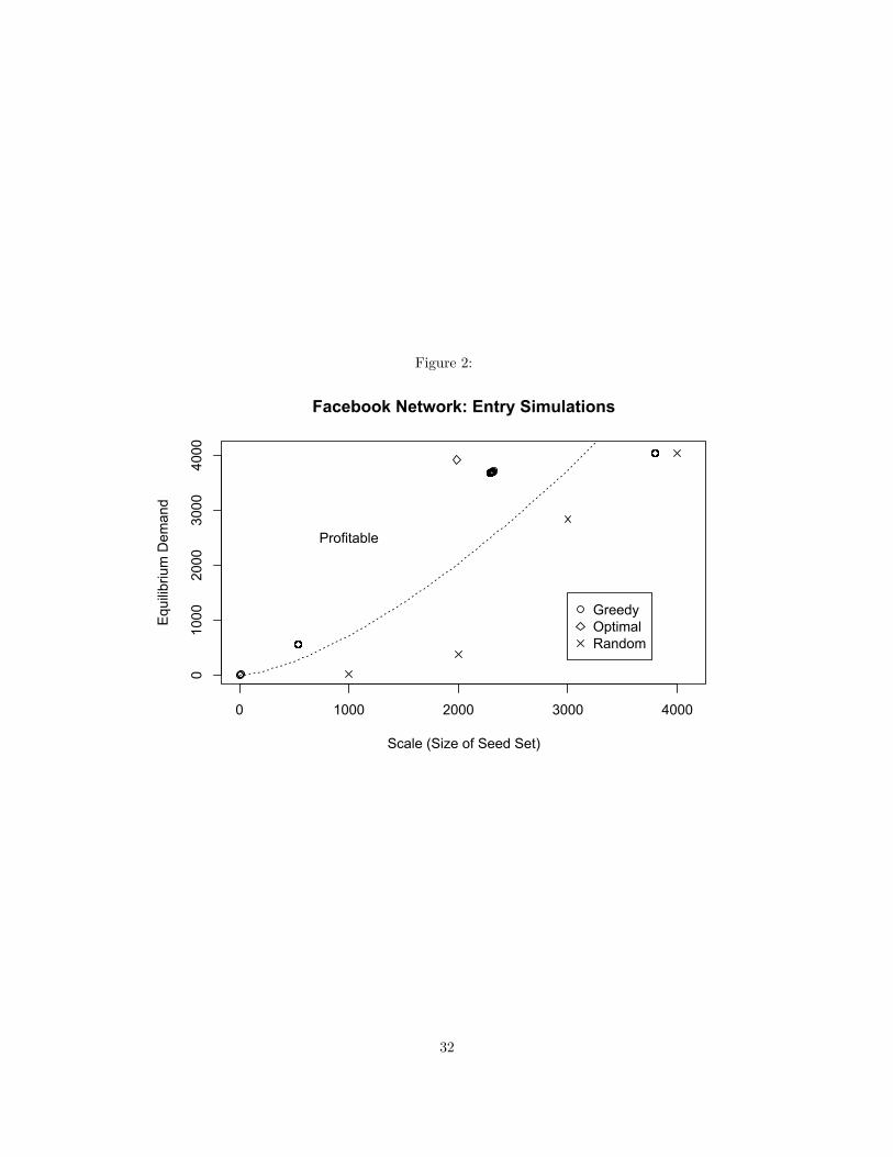
Figure 2:

0 1000 2000 3000 4000

010

0020

0030

0040

00

Facebook Network: Entry Simulations

Scale (Size of Seed Set)

Equ

ilibr

ium

Dem

and

GreedyOptimalRandom

Profitable

32

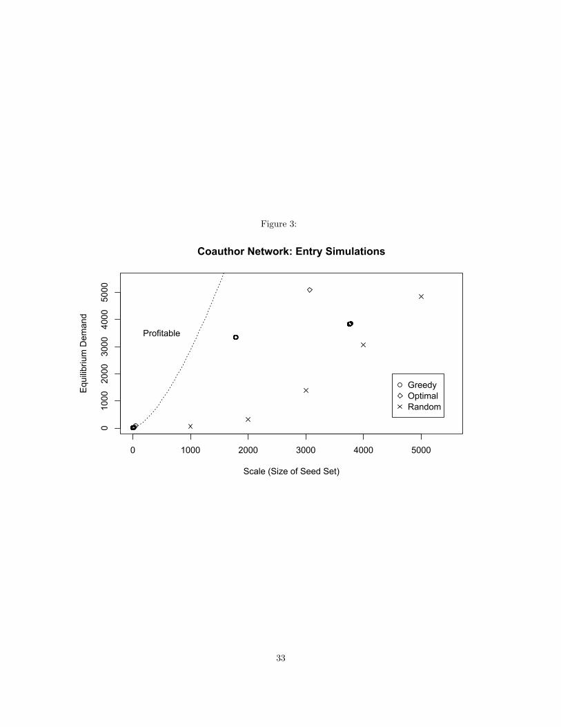
Figure 3:

0 1000 2000 3000 4000 5000

010

0020

0030

0040

0050

00

Coauthor Network: Entry Simulations

Scale (Size of Seed Set)

Equ

ilibr

ium

Dem

and

GreedyOptimalRandom

Profitable

33

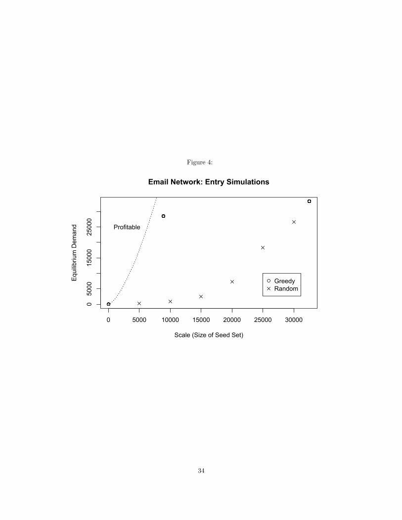
Figure 4:

0 5000 10000 15000 20000 25000 30000

050

0015

000

2500

0

Email Network: Entry Simulations

Scale (Size of Seed Set)

Equ

ilibr

ium

Dem

and

GreedyRandom

Profitable

34

In all the networks studied, the minimal scale needed to enter profitably was less than the scale needed to

enter an equivalent complete network (n/2). In the case of Facebook (Figure 2), the minimal scale was 4; for

the coauthor network (Figure 3) it was 2; and for the email network (Figure 4) it was 3. Barriers-to-entry,

calculated using the cost function above, were thus 8, 2.8, and 5 respectively; in contrast, barriers-to-entry

for an equivalent complete network with an equal number of nodes would be 90889, 134261, and 2485121

respectively.

From 200 trials of the greedy seeding algorithm, we see that the percentage of profitable trials were

52, 28, and 14 respectively. In other words, lean entry in the Facebook network was the most frequently

profitable of the three networks studied. There are two reasons for this. First, the frequency of t-cohesive

sets in the network determines profitability. Clusters of outcomes of the greedy algorithm indicate t-cohesive

sets found by this algorithm (due to the random nature of the algorithm, there are some slight random

variations between the sets). All three networks had a number of t-cohesive sets, but Facebook had 4 unique

clusters while the coauthor and email network both had 3. Second, the distribution of degrees in the network

determines profitability, with higher degree consumers being more profitable. This is easy to understand

because higher degrees results in greater externalities and more value generated from adoption. The Facebook

network has higher average degree and lower proportional variance than the other networks. Finally, the

network’s diffusiveness determines profitability. If we measure diffusiveness as the ratio of scale to equilibrium

demand, the email network appeared to be the most diffusive, with a demand of approximately 28K reached

from a scale of approximately 9K. However, its diffusiveness did not compensate for its comparatively low

average degree and high degree variance.

From 10 trials of the optimal seeding algorithm, we see that the algorithm had poor performance on the

coauthor network but was profitable for Facebook (Figure 2). The table below shows the best trial of the

greedy algorithm as the “optimal” profit for the email network. Note that in all three cases, optimal profit in

a complete network of equivalent size is vastly more profitable than optimal profit in the incomplete network

(the reverse is true with sharper cost functions, as indicated by Proposition 4.6). This is due to the vastly

higher average degree of the equivalent complete network: 4040, 5241, and 36691 respectively. However, we

would probably observe more frequent entry in the incomplete networks if resource-constrained firms are

unable to seed the minimal scale required to overcome barriers-to-entry in a complete network.

35

4.5.3 Diffusion and First Mover Advantage

So far, we have assumed in our analysis that the entrant firm is a second mover, and all consumers have

adopted an incumbent network good at the time of entry. This assumption is easily generalized to allow a

proportion of consumers to have adopted a non-network good at the time of entry. In this case, barriers-

to-entry are weaker. This is because a consumer with more peers adopting an incumbent network good

always has a weakly higher adoption threshold compared to if she had fewer peers. Though the principles

of t-cohesion still apply, lower thresholds make seeding less costly. Growth also occurs faster, meaning that

DP requires fewer iterations to reach equilibrium demand. In the extreme, if the firm is a first mover, the

smallest self-sustaining set contains only two members.

To formalize this observation, suppose y∗i = 1 if consumer i has adopted the incumbent’s good at time

of entry and y∗i = 0 if i has adopted a non-network good with quality θ. The entrant firm, as before, seeds

state x. Recall from section 4.2 that consumers have thresholds ti = vi−θα , where vi is the value of consumer

i’s outside option.

For consumer i who has adopted the incumbent’s good at time of entry, her outside option has value

vi = θ + α∑j∈L(i)(y

∗j − xj) and thus her adoption threshold is:

tτi =∑j∈L(i)

(y∗τj − xτj ) (9)

where y∗τj or xτj are equal to 1 if peer j adopts the incumbent’s or entrant’s good in an iteration of diffusion

τ . If y∗1j = 1 for all j ∈ L(i), this translates to the 12 proportional threshold we saw earlier: a consumer

adopts the entrant’s good if more than half her peers have already adopted.

For a consumer who has not adopted the incumbent’s good at time of entry, her outside option has value

vi = θ and thus her adoption threshold is ti = 0. This implies that a consumer of a non-network outside

option needs only one peer to adopt for the pair’s adoption to be self-sustaining.

Therefore the entrant’s start-up costs weakly increase in the market’s adoption of the incumbent’s good

at time of entry, y∗ = (y∗1 , . . . , y∗n), because it takes weakly more early adopters ||x|| to reach the same

demand.

36

Proposition 4.7. For any seed state x, demand D(x) for the entrant’s good is weakly lower when adoption

of the incumbent’s good is greater at time of entry:

If y∗ � y∗′ then D(x|y∗) ≤ D(x|y∗′).

Proposition 4.7 implies that given two identical network markets, a firm should enter the one where

fewer consumers have adopted an incumbent good. Of course, the decision of which market to enter in

reality requires many more trade-offs than the model addresses, including the cost of product development,

resources of incumbent firms, and so on, which are outside the scope of this paper. However, the theory does

suggest that the speed of late entry is important, and that becoming a first mover through radical innovation

may be more profitable than displacing incumbents through incremental innovation.

Ironically, complete network markets are actually ideal for diffusion if the firm is a first mover since

any two consumers form a self-sustaining set. DP requires only one iteration for adoption to diffuse to the

entire network, reflecting the tipping phenomenon of classic network effects theory. The result also holds

for bipartite markets where all consumers on one side are linked to all other consumers on the other side.

Combined with the observation that complete network markets can be more profitable due to a greater

number of externalities, this implies that a first mover given the option to enter a complete network market

should not use a lean entry strategy.

4.6 Discussion

The model in this chapter showed that barriers-to-entry in markets with network effects may be weaker

than previously characterized. The minimal scale needed to enter depends on the network structure of

externalities between consumers: the structural property of cohesion lowers minimal scale. But cohesion

is also a double-edged sword, stifling diffusion when too severe. Early adopters which span the boundary

between cohesive adopters and the rest of the network help balance this tension. In incomplete network

markets with a large fraction of “boundary spanners,” seeding a small number of early adopters can lead to

growth that is rapid and discontinuous. This is the core insight behind the strategy of lean entry.

A lean entry strategy can even the playing field between established firms and entrepreneurs. If en-

trepreneurs face resource constraints when seeding early adopters, it can be the only viable entry strategy.

Even in the absence of resource constraints, a lean entry strategy can be more profitable than alternatives

when the cost of seeding grows quickly in the number of early adopters. Its likelihood of profitability can

be predicted with simulations on real-world network data; for one of our networks lean entry was profitable

over 50 percent of the time.

37

Sometimes, employing a lean entry strategy may lead to lost opportunities. Becoming a first mover in a

new network market may be far more profitable than displacing an incumbent in an established one. In the

real world, firms may also have endogeneous influence over network structure. Though outside the scope of

our model, future research might explore how firms can design optimal network markets to build a competitive

advantage. For example, a firm might first enter an incomplete network and later increase the density of

externalities to strengthen barriers-to-entry against new entrants. Anecdotal evidence suggests some firms

have already implemented such practices, whether intentionally or by trial-and-error. For example, though

Facebook entered its market by way of college students, it quickly evolved into a two-sided platform linking

users, application developers, and advertisers.

38

5 First Mover Advantage of Exchange-Traded Products

5.1 Introduction

Exchange-traded products hold over $1.5T investor funds in the U.S. and have experienced tremendous

growth and innovation over the last decade. These products include exchange-traded funds (ETFs), struc-

tured as open-ended investment companies, and exchange-traded notes (ETNs), structured as debt securities.

Like mutual funds, ETPs allow investors to track an index, commodity, or basket of assets; like stocks, shares

of ETP also trade on US equity exchanges. For example, an ETF holding gold as its underlying asset enables

participants of the New York Stock Exchange to buy or sell gold by trading shares of the ETF.

Because of the products’ popularity and ease of imitation, the ETP industry tends to be intensely com-

petitive. This pattern of innovation followed by free entry has led to led most ETPs to become commodities

with arguably little to no product differentiation within markets. For example, several firms have issued gold

ETFs, both holding nearly identical underlying assets, i.e. gold bars kept in high-security vaults. At first

glance, it appears an investor can just as easily buy one gold ETF as another, and would thus pick the one

with the lowest price, known as an ETP’s expense ratio.

Yet puzzling performance differences persist between competing products. GLD and IAU, two nearly

identical gold ETFs both holding gold and trading on the same equity exchange, show a large disparity in

their assets under management (AUM), a proxy measure for investor demand. GLD, the first mover in this

market, has historically held over 80% of the total market AUM while charging higher expense ratios than

IAU.

These persistent performance differences are typical across ETP markets. Industry experts believe they

are caused by a first mover advantage. The ETP industry offers an unprecedented setting to test theories of

first mover advantage, due to both the sheer number of markets and amount of observable data within each

market. This allow an improved empirical design in at least three dimensions. First, while product failures

(exits) may not be observable in most industries, historical stock data is free of this selection bias as it tracks

the precise dates of ETP entry and exit. Second, ETPs competing within the boundaries of a market are

nearly identical in composition, providing a natural control for unobserved product differentiation. Moreover,

any remaining quality differences are observable, as product composition is clearly stated in fund prospectuses

and regulated by the SEC. Finally, since most firms issue many products, unobserved heterogeneity at the

firm level can be removed from measurements of first mover advantage at the product level.

I exploit these institutional features to test for the existence of first-mover advantage of ETPs. The

39

unit of observation is a product rather than a firm. ETP performance is measured by AUM and likelihood

of survival relative to competitors within a market. I estimate the impact of being a first mover on ETP

performance across approximately 300 markets while controlling for firm and cohort fixed effects, and find a

large and statistically significant impact which can be interpreted as causal.

I hypothesize that three mechanisms may drive first mover advantage at the product level: liquidity,

switching costs, and firm strategy. Analogous to network effects, investors’ preference for liquidity can cause

adoption for an incumbent product to snowball while creating barriers against new entrants. Switching costs

may drive first mover advantage if investors incur significant capital gains taxes, brokerage fees, or search

costs by switching to a competing product. They can also reinforce barriers to entry caused by liquidity.

Finally, the interaction between firm strategy and a product’s order of entry may drive first mover advantage

if firms learn or are able to capture superior resources when launching first mover products.

5.2 Literature

A longstanding aim of research in strategic management is to explain why some firms earn supranormal

profits compared to industry benchmarks. At one end of the debate, scholars in strategic management have

focused on features of firms themselves such as leadership, resource acquisition, and organizational structure.

At the other end, scholars have focused on features of markets and industrial organization such as market

structure, competitive positioning, and order of entry.

The order of entry framework used to explain firms’ supranormal profits is also known as the theory of

“first mover advantage.” According to this framework, first mover firms tend to become the “dominant”

firms in the industry. Scholars have introduced a multitude of theories to explain first mover advantage,

including pricing and output (Stackleberg 1934), learning and experience ( [6] [42]), product proliferation

(Hotelling 1929), switching and search costs ( [32], [18], [43]), technological advantages [35], and network

effects ( [17], [31]).

Empirical studies of first mover advantage have reached contrasting conclusions. In support of the theory,

scholars have shown learning [27], product proliferation and branding ( [40], [41], [25], [9]), search costs [24],

and supply-side economies of scale [45] to lead to superior first mover performance. But other studies have

been inconclusive and even shown evidence for a first mover disadvantage ( [21], see [39] for a survey). To

date, there is still insufficient evidence for first mover advantage as a general phenomenon across markets and

industries, in part because of methodological limitations such as survivorship and sampling bias, unobserved

firm-level heterogeneity, and lack of controls for firm tenure (see [47] for a meta-analysis).

40

My paper attempts to extend and clarify work in the first mover advantage literature by first testing

for first mover advantage in a novel industry where many of these confounders are directly observable,

and second, developing a novel empirical framework which exploits institutional features to help control for

product and firm-level heterogeneity.

My paper attempts to speak to a parallel but related literature which has held an ongoing debate about

the sustainability of competitive advantage. This literature researches whether competitive advantage, such

as that provided by first mover advantage, can be preserved or is necessarily competed away over time.

On the pro side of the debate, scholars have made two arguments in favor of sustainability: that a firm’s

institutional context, such as its culture and network, allows it to sustain a competitive advantage [37]; and

that sustainable competitive advantage is driven by resources that are valuable, scarce, and difficult to copy,

including intangible resources such as brand [11] [38] [22]. More recent work in this literature has focused

on identifying barriers to imitation. My paper may provide a particularly interesting contribution to this

debate since it finds evidence of sustainability, but appearing in a context where intellectual property is

highly transparent and easily imitable.

The final stream of literature my paper speaks to is the literature on innovation and competition in the

finance industry. Prior work from this literature focuses on firm incentives to innovate, such as risk sharing,

incomplete markets, agency issues, transaction costs, and response to regulation 5. However, I believe there is

much more to be found. To date, few studies have studied competition in financial industries; given the public

data sources available, this remains an untapped source of insights for the field of strategic management.

5.3 Empirical Design

5.3.1 Data

Two data sets were created for the purposes of this study. The first is a cross-sectional data set of the

performance and attributes of approximately 1700 ETPs across approximately 300 markets (henceforth

called ”markets”). Cross-sectional data was collected in December 2013. The second is a panel data set

tracking the entry, exit, and performance of these ETPs over time (henceforth called panel). I used the

markets data set to measure differences in equilibrium performance between first and late movers in the

same market, whereas I used the panel data to measure differences in ETP survival rates and growth.

To build these data sets, I combined and cross-validated data from the Center for Research in Security

Prices (CRSP) stock files, the CRSP mutual fund database, Bloomberg, Morningstar, and the SEC Edgar

5For a survey, see Allen & Gale (1994) [3], Duffie & Rahi (1995) [12], and Tufano (2003) [46]

41

database. CRSP stock header files tracked ETP performance, including AUM, trading volume, and entry

and exit. The CRSP mutual fund database, Bloomberg, and Morningstar track data on product attributes

such as expense ratios, portfolio holdings, and fund structure. In addition, Bloomberg and Morningstar

include ETP market specifications which formed the basis of my construct of market boundaries.

To create market boundaries, I first identified market boundaries by matching ETP product attributes

from the CRSP mutual fund database as well as product categories from Bloomberg and Morningstar. Each

ETP was labeled with 4 attributes: type (fund or note), leverage factor (-1 for inverse ETPs, 2 for 2x

leveraged ETPs, etc.), category (based on Bloomberg and Morningstar product categories), and category

refinement (based on string matching of CRSP product attributes). I then labeled two ETPs as belonging

to the same market if and only if they shared all 4 attributes. Table 2 contains examples of the final 10

largest and smallest ETP markets.

Next, I assigned a launch order to every ETP within a given market by ordering ETPs by their inception

date as determined by the first day of trading on an equity exchange. I assigned an order of 1 to the earliest

ETP in a market, 2 to the second, and so on. If two ETPs have the same inception date, they received the

same launch order. An ETP was labeled as a first mover if its launch order was 1. For a visual illustration

of this process, please see Figure 11 in the Appendix.

To filter for observations of equilibrium performance, I dropped markets that had less than two ETPs

competing within its boundaries, and markets which had been formed after 2011. For the remaining markets,

I calculated assets under management (AUM) by multiplying equilibrium (December 2013) outstanding

shares by share prices (net asset value or NAV). I calculated notional trading volume by multiplying the

number of traded shares by share prices. I calculated market shares by scaling an ETP’s AUM by the total

market’s AUM.

To create the panel data set, I used monthly outstanding shares and share prices from the CRSP stock

file from January 1993 to December 2013. Survival was calculated by identifying whether an ETP’s end date

of trading on an exchange was before December 2013. Growth rates over τ periods were calculated from

AUM observed in months t and t + τ . In addition, I collected a monthly panel of historical expense ratios

from the Morningstar ETF database.

To identify important historical events and changes in industry structure or regulations I used qualitative

data from SEC filings such as shareholder reports and investor prospectuses. Where useful I supplemented

this with sources such as Wall Street Journal, the Financial Times, and Harvard Business School cases.

There were some minor issues with missing data. 16 ETPs had missing expense ratios because they

42

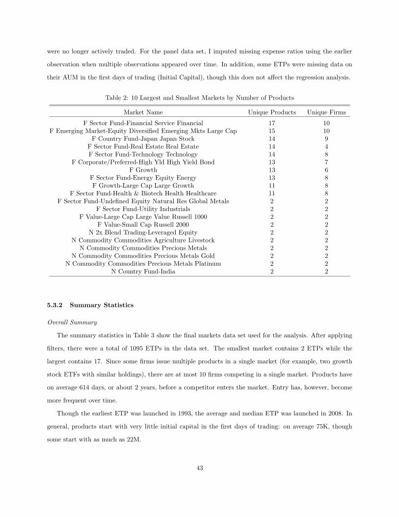
were no longer actively traded. For the panel data set, I imputed missing expense ratios using the earlier

observation when multiple observations appeared over time. In addition, some ETPs were missing data on

their AUM in the first days of trading (Initial Capital), though this does not affect the regression analysis.

Table 2: 10 Largest and Smallest Markets by Number of Products

Market Name Unique Products Unique Firms

F Sector Fund-Financial Service Financial 17 10F Emerging Market-Equity Diversified Emerging Mkts Large Cap 15 10

F Country Fund-Japan Japan Stock 14 9F Sector Fund-Real Estate Real Estate 14 4F Sector Fund-Technology Technology 14 8

F Corporate/Preferred-High Yld High Yield Bond 13 7F Growth 13 6

F Sector Fund-Energy Equity Energy 13 8F Growth-Large Cap Large Growth 11 8

F Sector Fund-Health & Biotech Health Healthcare 11 8F Sector Fund-Undefined Equity Natural Res Global Metals 2 2

F Sector Fund-Utility Industrials 2 2F Value-Large Cap Large Value Russell 1000 2 2

F Value-Small Cap Russell 2000 2 2N 2x Blend Trading-Leveraged Equity 2 2

N Commodity Commodities Agriculture Livestock 2 2N Commodity Commodities Precious Metals 2 2

N Commodity Commodities Precious Metals Gold 2 2N Commodity Commodities Precious Metals Platinum 2 2

N Country Fund-India 2 2

5.3.2 Summary Statistics

Overall Summary

The summary statistics in Table 3 show the final markets data set used for the analysis. After applying

filters, there were a total of 1095 ETPs in the data set. The smallest market contains 2 ETPs while the

largest contains 17. Since some firms issue multiple products in a single market (for example, two growth

stock ETFs with similar holdings), there are at most 10 firms competing in a single market. Products have

on average 614 days, or about 2 years, before a competitor enters the market. Entry has, however, become

more frequent over time.

Though the earliest ETP was launched in 1993, the average and median ETP was launched in 2008. In

general, products start with very little initial capital in the first days of trading: on average 75K, though

some start with as much as 22M.

43

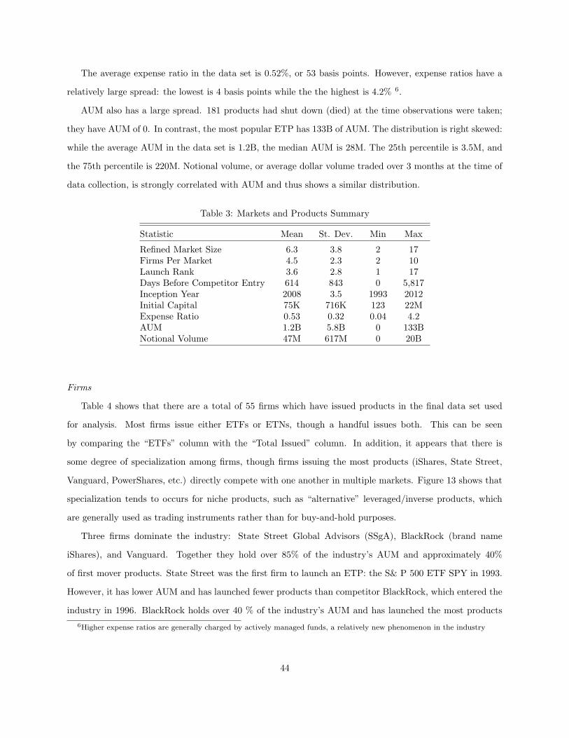
The average expense ratio in the data set is 0.52%, or 53 basis points. However, expense ratios have a

relatively large spread: the lowest is 4 basis points while the the highest is 4.2% 6.

AUM also has a large spread. 181 products had shut down (died) at the time observations were taken;

they have AUM of 0. In contrast, the most popular ETP has 133B of AUM. The distribution is right skewed:

while the average AUM in the data set is 1.2B, the median AUM is 28M. The 25th percentile is 3.5M, and

the 75th percentile is 220M. Notional volume, or average dollar volume traded over 3 months at the time of

data collection, is strongly correlated with AUM and thus shows a similar distribution.

Table 3: Markets and Products Summary

Statistic Mean St. Dev. Min Max

Refined Market Size 6.3 3.8 2 17Firms Per Market 4.5 2.3 2 10Launch Rank 3.6 2.8 1 17Days Before Competitor Entry 614 843 0 5,817Inception Year 2008 3.5 1993 2012Initial Capital 75K 716K 123 22MExpense Ratio 0.53 0.32 0.04 4.2AUM 1.2B 5.8B 0 133BNotional Volume 47M 617M 0 20B

Firms

Table 4 shows that there are a total of 55 firms which have issued products in the final data set used

for analysis. Most firms issue either ETFs or ETNs, though a handful issues both. This can be seen

by comparing the “ETFs” column with the “Total Issued” column. In addition, it appears that there is

some degree of specialization among firms, though firms issuing the most products (iShares, State Street,

Vanguard, PowerShares, etc.) directly compete with one another in multiple markets. Figure 13 shows that

specialization tends to occurs for niche products, such as “alternative” leveraged/inverse products, which

are generally used as trading instruments rather than for buy-and-hold purposes.

Three firms dominate the industry: State Street Global Advisors (SSgA), BlackRock (brand name

iShares), and Vanguard. Together they hold over 85% of the industry’s AUM and approximately 40%

of first mover products. State Street was the first firm to launch an ETP: the S& P 500 ETF SPY in 1993.

However, it has lower AUM and has launched fewer products than competitor BlackRock, which entered the

industry in 1996. BlackRock holds over 40 % of the industry’s AUM and has launched the most products

6Higher expense ratios are generally charged by actively managed funds, a relatively new phenomenon in the industry

44

as well as the most first movers. A visualization appears in Figure 12 in the Appendix. Vanguard entered

the industry in 2001. Though a late entrant with comparatively few products and few first movers, it has a

disproportionate amount of AUM.

45

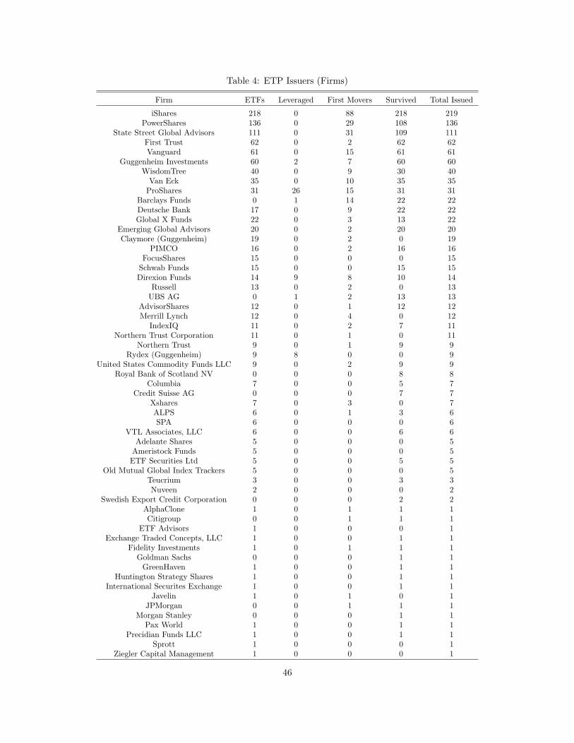
Table 4: ETP Issuers (Firms)

Firm ETFs Leveraged First Movers Survived Total Issued

iShares 218 0 88 218 219PowerShares 136 0 29 108 136

State Street Global Advisors 111 0 31 109 111First Trust 62 0 2 62 62Vanguard 61 0 15 61 61

Guggenheim Investments 60 2 7 60 60WisdomTree 40 0 9 30 40

Van Eck 35 0 10 35 35ProShares 31 26 15 31 31

Barclays Funds 0 1 14 22 22Deutsche Bank 17 0 9 22 22Global X Funds 22 0 3 13 22

Emerging Global Advisors 20 0 2 20 20Claymore (Guggenheim) 19 0 2 0 19

PIMCO 16 0 2 16 16FocusShares 15 0 0 0 15

Schwab Funds 15 0 0 15 15Direxion Funds 14 9 8 10 14

Russell 13 0 2 0 13UBS AG 0 1 2 13 13

AdvisorShares 12 0 1 12 12Merrill Lynch 12 0 4 0 12

IndexIQ 11 0 2 7 11Northern Trust Corporation 11 0 1 0 11

Northern Trust 9 0 1 9 9Rydex (Guggenheim) 9 8 0 0 9

United States Commodity Funds LLC 9 0 2 9 9Royal Bank of Scotland NV 0 0 0 8 8

Columbia 7 0 0 5 7Credit Suisse AG 0 0 0 7 7

Xshares 7 0 3 0 7ALPS 6 0 1 3 6SPA 6 0 0 0 6

VTL Associates, LLC 6 0 0 6 6Adelante Shares 5 0 0 0 5

Ameristock Funds 5 0 0 0 5ETF Securities Ltd 5 0 0 5 5

Old Mutual Global Index Trackers 5 0 0 0 5Teucrium 3 0 0 3 3Nuveen 2 0 0 0 2

Swedish Export Credit Corporation 0 0 0 2 2AlphaClone 1 0 1 1 1Citigroup 0 0 1 1 1

ETF Advisors 1 0 0 0 1Exchange Traded Concepts, LLC 1 0 0 1 1

Fidelity Investments 1 0 1 1 1Goldman Sachs 0 0 0 1 1

GreenHaven 1 0 0 1 1Huntington Strategy Shares 1 0 0 1 1

International Securites Exchange 1 0 0 1 1Javelin 1 0 1 0 1

JPMorgan 0 0 1 1 1Morgan Stanley 0 0 0 1 1

Pax World 1 0 0 1 1Precidian Funds LLC 1 0 0 1 1

Sprott 1 0 0 0 1Ziegler Capital Management 1 0 0 0 1

46

Competition and Industry Growth

The ETP Industry overall has grown rapidly. A visualization appears in Figure 10 in the Appendix. The

growth of the industry has led to a greater frequency of entryover time. For example, Table 5 shows that

while the median duration before competitor entry was roughly 5.5 years for an ETP launched before 2000,

the duration was reduced to a mere 3 months by 2011. The number of products launched overall increased

sharply around 2005. Overall industry growth is also reflected in the time it takes before a second mover

enters the market compared to a third or fourth mover, though there, strategic factors are also likely at play.

Table 5: Days Before Competitor Entry by Inception Year

Min. 1st Qu. Median Mean 3rd Qu. Max.

Before 2000 84 544 2, 051 2, 439 4, 413 5, 8172001 84 1, 077 1, 587 1, 588 1, 796 3, 5422002 0 472 1, 526 1, 323 1, 754 3, 3812003 42 919 1, 201 1, 454 2, 286 2, 7972004 64 201 630 631 886 2, 5562005 13 178 329 610 774 2, 2882006 0 31 172 475 642 2, 3162007 0 72 202 446 754 1, 9922008 0 237 665 671 1, 092 1, 6682009 0 134 308 363 533 1, 1622010 0 36 193 221 348 9862011 0 24 85 168 282 694

Table 6: Days Before Competitor Entry by Order of Entry

Order of Entry Min. 1st Qu. Median Mean 3rd Qu. Max.

1st 0 139 472 956 1, 547 5, 8172nd 0 91 311 614 886 3, 7603rd 0 90 301 527 790 2, 6934th 0 54 176 420 671 1, 878

47

In general, larger markets (as measured by total market AUM, a proxy for total demand) experience more

entry. For example, Table 7 shows that markets with 2 or 3 entrants have lower total AUM than markets

with 4 or more entrants. However, demand appears to be distributed unevenly across competitors. There is

a sizeable difference in AUM between a market’s first and second mover, and this difference does not appear

to narrow based on the size of the market.

The difference in performance between early and late movers appears to hold more generally. Figure

5 shows that a product’s order of entry appears to have a strong correlation with its AUM: on average,

first movers seem to have significantly greater AUM than late movers (note the linear relationship in logs).

Again, it is worthwhile to emphasize this pattern does not appear to be driven by market size; it is not

merely the case that larger markets invite more entry and thus each late entrant receives an evenly smaller

market share.

Table 7: AUM by Market Size

Market Size Number of Markets Avg. Market AUM logAUM 1st Mv. - logAUM 2nd Mv.

2 88 1.1B 16.8843 49 3.4B 16.8744 37 10.2B 18.4975 23 5.1B 18.4046 17 8.7B 16.7417 8 3.8B 13.1768 8 10.1B 19.7899 7 8.4B 19.26310 7 7.3B 12.91211 5 9.1B 20.06313 3 14.1B 19.35414 3 8.5B 18.65115 1 64.8B 22.06317 1 14.1B 20.240

48

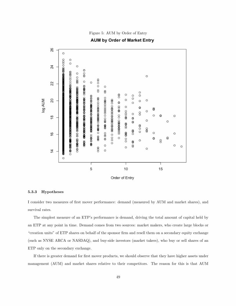
Figure 5: AUM by Order of Entry

5.3.3 Hypotheses

I consider two measures of first mover performance: demand (measured by AUM and market shares), and

survival rates.

The simplest measure of an ETP’s performance is demand, driving the total amount of capital held by

an ETP at any point in time. Demand comes from two sources: market makers, who create large blocks or

“creation units” of ETP shares on behalf of the sponsor firm and resell them on a secondary equity exchange

(such as NYSE ARCA or NASDAQ), and buy-side investors (market takers), who buy or sell shares of an

ETP only on the secondary exchange.

If there is greater demand for first mover products, we should observe that they have higher assets under

management (AUM) and market shares relative to their competitors. The reason for this is that AUM

49

measures the total investor funds held by an ETP, plus investment returns. Since the returns of products

competing within a market are identical, demeaning AUM or calculating market share removes the effect of

fund returns and thus only measures demand from market participants.

Another measure of an ETP’s performance is survival. ETP survival is often a reasonable proxy for

profits, as firms generally shut down a product when it is unprofitable. Thus if first mover ETPs are more

profitable than competitors, we should observe that they have a higher likelihood of survival.

An product’s profitability is generally determined by two factors: its revenue to the issuing firm, and

variable costs. The majority of revenue derives from the expense ratio charged to investors as a percentage

of AUM. A small amount of revenue also comes from fees charged to market makers. Variable costs of

managing an ETP include custodian fees, manager salaries, transaction costs from rebalancing holdings, and

profit sharing with distributors and affiliates.

Since we cannot observe all variable costs, we cannot measure an ETP’s exact profits. But a rule of

thumb proposed by industry experts is that it takes $20M − $30M of AUM for a product to survive. Using

average industry expense ratios, we can back out variable costs to be approximately $100K annually, though

larger ETP issuers likely incur lower costs.

Several factors may explain why first mover products perform better than market benchmarks. Many do

not reflect a true first mover advantage, as they are not causally driven by a product’s order of entry. Such

spurious drivers of “first mover advantage” include price and product differentiation exogenous to order of

entry, differences in product tenure, and firm heterogeneity.

Despite these caveats, a first mover advantage does appear plausible in the ETP context. Moreover,

due to the availability of data on expense ratios (price), product composition (by definition nearly identical

within market boundaries), product inception dates, and issuing firms, we can remove much of the spurious

causes of superior first mover performance listed above. I thus hypothesize:

Hypothesis 5.1. First mover exchange-traded products (ETPs) have higher equilibrium AUM, market

shares, and survival rates than competitors. Moreover, these performance differences are not driven by

product differentiation, expense ratios (price), differences in product tenure, or firm heterogeneity.

To test this hypothesis, I estimate a firm and market fixed-effects model of log AUM as a function of

a first mover dummy and product-level controls. In order to interpret the coefficients on first mover as a

causal measure, my empirical design assumes that all differences in ETP performance within a market are

due to order of entry after accounting for firm fixed effects, market fixed effects, and controls.

50

Controls include equilibrium expense ratios (Expensei) and product tenure (inception year dummies Yi).

Adding market fixed effects implicitly controls for product differentiation. As a robustness check that market

boundaries are correctly drawn and thus adequately control for product differentiation, I estimate the model

using only products tracking the same indices (thus having identical composition by definition).

I also estimate a model of AUM market share Sharei as a function of a first mover dummy, firm fixed

effects, firm-first mover interactions, and controls. To calculate market share, I divide the AUM of an

individual ETP i by the total AUM of all ETPs in i’s market and multiply by 100.

Finally, I estimate a logit model of ETP survival Survivei, where survival is defined by whether an ETP

has positive AUM in equilibrium. I use the same independent variables and controls as in the models above,

but use only firm fixed effects since there is no reason to assume inherent differences in survival rates across

markets.

Regression specifications appear below, where ρ is the coefficient of interest. The subscript i indicates

an ETP, Firsti is a first mover dummy, Firsti ∗ Fi is a firm-first mover interaction, Fi is firm fixed effects,

Mi is market fixed effects, Expensei is expense ratio, and Yi is inception year:

log(AUMi) = β0 + ρF irsti + β1Expensei + β2Yi + Fi +Mi + εi (10)

Sharei = β0 + ρF irsti + β1Expensei + β2Yi + Fi + εi (11)

Logit(Survivei) = β0 + ρF irsti + β1Expensei + β2Yi + Fi + εi (12)

5.4 Results

Consistent with hypothesis 5.1, I find that first mover ETPs have several times greater AUM, market share,

and likelihood of survival than market competitors. These performance differences persist even when account-

ing for product differentiation, expense ratios (price), differences in product tenure, and firm heterogeneity.

As stated in the table 8 below, first mover ETPs have approximately 5 times higher AUM than late movers

in their respective markets. If all spurious drivers of first mover performance are indeed fully accounted by

product differentiation, expense ratios, differences in product tenure, and firm heterogeneity, this bump

in AUM can be interpreted as the magnitude of first mover advantage from a demand perspective: first

movers are on average 5 times more in demand than late movers. A 95% confidence interval, while large

51

(apprxoimately 2 - 10 times higher AUM), is significantly different from 0.

Similarly, first mover ETPs show approximately 45% greater market share than late mover competitors.

A 95% confidence interval is approximately 41% - 49% and is significantly different from 0. Again we can

interpret this figure as an estimate of first mover advantage from a demand perspective if our controls account

for spurious drivers of first mover performance.

Finally, first mover ETPs have approximately 4 times higher odds of survival than their late mover

counterparts. The odds ratio can be calculated precisely by exponentiating the coefficient in table 8. A 95%

confidence interval is approximately 2.5 - 6 times greater odds of survival, again significantly different from

0. We can interpret this figure as an indication of first mover advantage from an operating profit perspective

if our controls account for spurious drivers of first mover performance. It does not indicate whether this

bump in operating profit is depleted by differences in fixed costs when launching first versus late movers.

Table 8: First Mover Performance: AUM, Market Share, and Survival

Dependent variable:

Fixed Effects Fixed Effects Logistic

log AUM Market Share Survive

(1) (2) (3)

First Mover 1.596∗∗∗ 0.453∗∗∗ 1.350∗∗∗

(0.383) (0.020) (0.473)

Expense Ratio −3.139∗∗∗ 0.031 −4.995∗∗∗

(0.851) (0.041) (1.168)

Inception Year −0.313∗∗∗ −0.002 −0.002(0.065) (0.003) (0.096)

Firm FE Y Y Y

Market FE Y

Observations 1,079 1,065 1,079R2 0.699 0.508Adjusted R2 0.492 0.482Log Likelihood −136.365Akaike Inf. Crit. 382.729F Statistic 33.239∗∗∗ (df = 53; 760) 19.712∗∗∗ (df = 53; 1011)

Note: ∗p<0.1; ∗∗p<0.05; ∗∗∗p<0.01

Robustness Checks

52

While the differences between first and late mover performance appear large, these figures must be

interpreted with caution. If there are unobservable drivers of first mover performance which are not caused

by order of entry, these figures likely overstate the magnitude of first mover advantage due to omitted variable

bias. Although I accounted for the major spurious drivers of first mover performance noted by the theory

and past empirical studies of first mover advantage, my methodology cannot remove all bias.

To further test the extent to which the results above are valid, I run three robustness checks. First, I test

whether controlling for unobserved firm-level heterogeneity was important for removing endogeneity from the

First Mover coefficient. If unobserved firm-level factors such as strategy, branding, or operational efficiencies

is not important for AUM, then removing the firm fixed effect from regression 10 should not affect the First

Mover coefficient. I find evidence that adding this control does remove a portion of the endogeneity, as seen

by the lower mean coefficient and non-overlapping confidence intervals of First Mover in Table 9.

Next, I test for residual variation in the First Mover variable given all the controls in regression 10. If

there is little to no variation in the First Mover variable after accounting for controls; then the results of

Table 8 would be invalid due to collinearity. Table 10 shows that while there is some correlation between

First Mover status and controls, there is still variation in First Mover status after accounting for firms,

expense ratios, and inception year, as seen by the reasonably low R-squared of this test.

Finally, I test for remaining endogeneity in the First Mover variable by running the same analyses on

a subset of markets: those whose first mover experiences competitor entry in 1-90 days. Looking at this

subset of markets is interesting because for nearly identical products that are launched close together in

time, the First Mover coefficient should be more accurately measuring a First Mover Advantage, free from

endogenous drivers of first mover performance. For example, the disparity in performance of GLD and IAU,

which launched a month apart and both were issued by experienced firms who submitted their prospectus

to the SEC at nearly the same time, is likely wholly driven by a First Mover Advantage.

I find that, while the coefficient for Regression 10 is lower for this subset of ETPs, it is still positive

and significant at the 10 % level. Its confidence interval also overlaps with that of Table 8. The coefficient

for Regression 11 is also lower and has a confidence interval which does not overlap with that of Table 8;

however it is still positive and significant at the 1% level. Finally, the coefficient for Regression 12 shows

no significant difference, though a wider confidence interval due to the smaller sample size. The results of

this test suggest that, while there may be some level of endogeneity in the coefficients estimated above, it

more accurately represents a true First Mover Advantage rather than endogenous drivers of First Mover

performance. It is also interesting to note that the coefficient on Expense Ratio is greater for this subset of

53

ETPs, suggesting that price is a bigger driver of performance when consumer switching costs are less of an

issue.

54

Table 9: Test for Firm-level Heterogeneity

Dependent variable:

log AUM

(1) (2) (3)

First Mover 4.214∗∗∗ 2.070∗∗∗ 1.546∗∗∗

(0.475) (0.559) (0.379)

Expense Ratio −2.839∗∗∗ −2.911∗∗∗

(0.817) (0.813)

Inception Year −0.513∗∗∗ −0.296∗∗∗

(0.080) (0.061)

Firm Fixed Effects N N YMarket Fixed Effects Y Y Y

Observations 1,109 1,092 1,092R2 0.085 0.158 0.689Adjusted R2 0.065 0.120 0.492F Statistic 78.833∗∗∗ (df = 1; 851) 51.977∗∗∗ (df = 3; 832) 30.863∗∗∗ (df = 56; 779)

Note: ∗p<0.1; ∗∗p<0.05; ∗∗∗p<0.01

55

Table 10: Test for Variation in First Mover Status

Dependent variable:

First Mover

Expense Ratio 0.067(0.077)

Inception Year −0.092∗∗∗

(0.005)

Firm Fixed Effects Y

Market Fixed Effects Y

Observations 1,092R2 0.455Adjusted R2 0.325F Statistic 11.848∗∗∗ (df = 55; 780)

Note: ∗p<0.1; ∗∗p<0.05; ∗∗∗p<0.01

56

Table 11: Markets with 1-90 Days between First and Second Mover Entry

Dependent variable:

Fixed Effects Fixed Effects Logistic

log AUM Market Share Survive

(1) (2) (3)

First Mover 1.023∗ 0.286∗∗∗ 1.478∗

(0.573) (0.028) (0.859)

Expense Ratio −8.508∗∗∗ −0.228∗∗∗ −4.885∗∗∗

(1.483) (0.072) (1.460)

Inception Year −0.346∗∗∗ −0.020∗∗∗ 0.081(0.087) (0.004) (0.110)

Firm FE Y Y Y

Market FE Y

Observations 612 612 612R2 0.678 0.554Adjusted R2 0.507 0.554Log Likelihood −85.542Akaike Inf. Crit. 281.084F Statistic 17.856∗∗∗ (df = 54; 457) 10.492∗∗∗ (df = 54; 457)

Note: ∗p<0.1; ∗∗p<0.05; ∗∗∗p<0.01

57

5.5 Discussion

This paper shows evidence of superior first mover performance in the ETP industry. First movers have

greater demand (AUM), market share, and survival rates than their competitors. Moreover, this difference

in ETP performance appears to reflect a true first mover advantage rather than product differentiation,

expense ratios (price), differences in product tenure, or firm heterogeneity. The advantage has persisted, at

least for some products, over the course of decades.

These results offer two major contributions to scholarship. First is to provide a richer understanding of

the theory of first mover advantage in a novel empirical context and with a novel empirical design. The

empirical design in this paper attempts to remove many of the factors confounding prior studies of first

mover advantage, such as unobserved differences between firms and products, and survivorship bias. As far

as the researcher is aware, no previous research has studied first mover advantage at the product level. This

paper shows that such an empirical design may lead to more accurate and precise measurements of first

mover advantage than analysis at the firm level.

Second, this paper improves our understanding of innovation management and contributes to the sus-

tainability of competitive advantage debate. Though first mover advantage alone does not imply firms earn

supranormal returns to innovation, evidence of greater operating profits is consistent with the hypothesis

that innovation, at least in the context of financial products, leads to competitive advantage. Moreover, this

competitive advantage appears to be sustainable over the course of decades. Future work may estimate the

magnitude of returns to innovation and explore counterfactuals of how innovation incentives change with

respect to market or regulatory parameters.

This paper also has implications for firms competing in the ETP industry. Understanding the magnitude

of first mover advantage can help issuers of ETPs allocate resources more effectively for growth. My results

suggest that order of entry is an important factor to consider when launching ETPs. For regulators, the

magnitude of first mover advantage can provide a signal of socially suboptimal levels of innovation in the

ETP industry is socially suboptimal. For example, first mover advantage may lead to too much innovation

if the proliferation of new markets leads to greater investor search costs and a reduction in liquidity.

The finding of such a strong first mover advantage in the ETP industry merits further research to

determine its drivers. One likely driver of first mover advantage is product liquidity, which loosely speaking,

is the willingness of market participants to buy or sell an ETP at a particular point in time. Liquidity may act

as an investor coordination mechanism analogous to network effects. This may then create barriers-to-entry,

or what Duffie and Rahi (1995) [12] call “the preemptive value of liquidity.”

58

Investor switching costs can also drive first mover advantage. Transaction costs such as capital gains

taxes and brokerage fees may prevent investors from adopting a competitor’s product even if it has a lower

expense ratio. In addition, it may be costly for investors to assess the portfolio holdings, risks, and legal

structure of new ETPs. For example, Hortacsu and Syverson (2003) [24] attribute price dispersion in the

highly related mutual fund industry to search costs.

Other potential drivers of first mover advantage in the ETP industry include firm learning and strategy.

For example, firms become more effective at launching ETPs as they grow their product porfolio, R& D

and management costs may become lower with experience, or firms may learn to negotiate better deals with

ETP distributors. A firm may also strategically launch first movers, offering lower fees to market makers

because they expect higher buy-side investor demand, or preemptively securing scarce resources such as

popular stock indexes so that they are unavailable to late movers.

A particularly interesting example of an ETP issuer which has grown successfully despite entering late in

the industry is Vanguard. Vanguard was likely able to overcome first mover advantage due to three important

factors: its reputation for low-cost index investing, vast supply-side economies of scale, and the creation of a

new share class which effectively bundled ETPs with its standard mutual fund portfolio 7. The creation of

this share class allowed their existing investors to incur virtually no transaction costs when switching from

mutual funds to ETPs, thus seeding sufficient liquidity for the new products to take off.

7See HBS case study ”The Complexity of Vanguard’s Entry Decision into ETFs, 2014; by L. Cohen, C. Malloy, and T. Tang.

59

6 Growing Digital Content: the Case of Yelp.com

6.1 Introduction

This chapter investigates the growth of review aggregator Yelp.com, a socially-driven network good which

seems to have used a lean entry strategy.

Yelp, a review website for restaurants and small businesses, is one of many modern technologies which

relies on users as its primary producer of value. Other digital goods including content aggregators, social

media platforms, and open source software rely on users to generate information, profiles, or software, which

are then consumed by other users.

Despite the importance of user-generated content production for these digital goods, we know little

about the mechanisms by which content production grows. First, who are early producers of user-generated

content? Second, to what extent does early content production drive later content growth? Finally, what

does this imply for the strategic decision-making of a firm such as Yelp?

Using review data from Yelp.com from 2005 to 2014, this paper seeks to answer these questions. We find

that early producers of Yelp’s user-generated content were largely concentrated in a single city, but spillover

effects drove a large fraction early content production in other cities. The magnitude of the spillover is highly

correlated with the volume of tourism between cities. We also find that early reviews produced by tourists

is predictive of later review growth, more so than early reviews produced by local reviewers. We hypothesize

that the latter finding indicates the presence of a network effect.

6.2 History of Content Generation on Yelp

Yelp was founded in 2004 in San Francisco. During Yelp’s early growth period from January 2005 to March

2007, the website had over 30,000 reviewers. 16,000 of these reviewers were concentrated in San Francisco,

with less than 1000 total reviewers in most other U.S. cities.

Yelp’s entry strategy was to focus its marketing efforts on driving adoption in San Francisco prior to

March 2007 while relying on organic content growth in most other cities. 10 cities other than San Francisco

showed reviews during this period. Table 12 shows that of these, only four cities (Boston, Seattle, New York,

Los Angeles, and San Diego) had more than 1000 early reviewers. Yelp’s market penetration, measured as

the percentage of total historical reviewers, was less than 2 percent in most cities. Its percentage of historical

content generated prior to March 2007 was also less than 2 percent. Because company employees posted

restaurant listings in each city early on, the percentage of restaurants listed during this period was much

60

higher, at around 30 percent.

Who were early reviewers in these cities? Table 15 shows that a large percentage of early reviewers were

tourists from San Francisco. In most cities, less than half of all early reviewers were local residents of that

city. The remaining early reviewers were tourists from cities other than San Francisco. For example, and

tourists from San Francisco left 367 reviews for restaurants in Portland prior to March 2007, and tourists

from Seattle left 189 reviews.

Around March 2007, Yelp shifted its strategy to focus on national and later international expansion. For

example, Yelp begin to send direct mail to local businesses in cities outside of San Francisco. It also hired

what are known as “community managers,” local marketers who organize events aimed at increasing local

adoption. Starting around 2008, Yelp’s digital content grew quickly. Figure 6 shows the growth of total

reviews over time in each of the 11 cities with early adoption, including San Francisco.

61

Tab

le12

:Y

elp

’sG

row

thin

San

Fra

nci

sco

vers

us

10

Earl

yA

dop

tin

gU

.S.

Cit

ies

EarlyPeriod(1/2005-3/2007)

PercentofTotalHistoric

#R

esta

ura

nts

*M

onth

lyR

evie

ws

#R

evie

wer

s**

Res

tau

rants

*R

evie

ws

Rev

iew

ers*

*

San

Fra

nci

sco

2,7

36

20,7

99

16,1

90

56%

7%

5%

Bost

on

748

342

1,8

98

45%

4%

2%

Sea

ttle

1,3

11

397

1,8

10

40%

2%

1%

New

York

3,6

52

914

3,9

15

35%

2%

1%

LA

1,7

66

497

3,0

59

25%

1%

1%

Wash

ingto

nD

.C.

718

145

786

29%

1%

1%

Ph

ilad

elp

hia

612

74

403

19%

<1%

<1%

Las

Veg

as

501

85

869

14%

<1%

1%

San

Die

go

1,0

24

169

1,1

63

26%

<1%

1%

Ph

oen

ix321

31

221

14%

<1%

<1%

Port

lan

d619

71

466

20%

<1%

1%

*T

oacc

ou

nt

for

rest

au

rant

turn

over

,th

isfi

gu

reex

clu

des

rest

au

rants

inb

ott

om

25

per

centi

leof

revie

ws.

**A

nin

div

idu

al

wh

ore

vie

wed

at

least

1re

staura

nt

info

cal

city

.

62

Table 13: Composition of Early Reviewers

% Local % From SF

San Francisco 80% –

Boston 53% 12%

Seattle 55% 17%

New York 46% 22%

LA 52% 22%

Washington D.C. 38% 21%

Philadelphia 18% 22%

Las Vegas 4% 46%

San Diego 36% 27%

Phoenix 38% 24%

Portland 35% 34%

63

Figure 6: Yelp’s Content Growth

0

500000

1000000

1500000

2006 2008 2010 2012 2014Date

# R

evie

ws

citynameBoston, MA

Las Vegas, NV

Los Angeles, CA

New York, NY

Philadelphia, PA

Phoenix, AZ

Portland, OR

San Diego, CA

San Francisco, CA

Seattle, WA

Washington, DC

Cumulative Yelp Reviews, 2004 - 2014

64

6.3 Data and Hypotheses

Data

We gathered Yelp review data during the years 2005-2013, for restaurants in 11 major U.S. cities including

San Francisco. Review data contains the day, month, and year of review; the name, ID, self-reported

location, friends, and total reviews of the reviewer leaving the review; the name, ID, location, and genre

of the restaurant being reviewed; and attributes of the review itself such as star rating and content. We

choose to examine restaurants because they comprise the highest percentage (approximately 40 percent) of

businesses listed on Yelp prior to 2011. Since the restaurant industry is marked by frequent turnover, we

excluded restaurants in the bottom 25 percentile of reviews in each city.

In addition to Yelp review data, we gathered data on airport traffic from the Bureau of Transportation

Statistics. This data contains a record of every flight arriving or departing between two airports in a given

day (we aggregate it to the monthly level). The data also provides city names associated with each airport

code. City names from the flights data were linked to self-reported reviewer locations in the Yelp data by

relabeling locations with its corresponding metropolitan statistical area (MSA). For example, a review of a

New York City restaurant written by a reviewer in ”Cambridge, MA” would be relabeled ”Boston, MA” and

linked to all flights from Boston to New York City.

Tourists are identified by self-reported reviewer locations: a review is classified as “tourist” if and only

if the reviewer’s reported location is not contained within the metropolitan statistical area (MSA) of the

restaurant receiving the review. For example, if a reviewer from Cambridge, MA reviews a restaurant located

in Boston, MA, the review is labeled as a local review. If, on the other hand, a reviewer from New York,

NY reviews a restaurant in Boston, MA, the review is labeled as a tourist review.

Hypotheses

The production of content by tourists corresponds to a spillover effect, in the sense that the production

in one market had increased its production in adjacent markets. We hypothesize that the spillover effect

is large in magnitude and drove the majority of Yelp’s early content. To measure the magnitude of the

spillover, we count the total number of reviews written by tourists across the early adopter cities.

Hypothesis 6.1. Spillovers from tourism drove the majority of Yelp’s content production in cities outside

San Francisco prior to March 2007.

We are further interested in factors which might affect the magnitude of the spillover, especially those

that are strategically relevant to Yelp. We hypothesize that volume of tourism between cities is correlated

65

with the magnitude of the spillover. In particular, reviews written by tourists from city i to city j should

increase (decrease) if tourism from city i to city j increases (decreases). To measure tourism between cities,

we count the monthly number of flights arriving from city i to city j.

Hypothesis 6.2. The average number of Yelp reviews written by tourists from city i for a restaurant located

in a city j increases (decreases) as the number of flights from city i to city j increases (decreases).

To test hypothesis 6.2, we run a regression with year-month and city j fixed-effects:

Yijt = ρXijt + Tt + Cj + εijt (13)

where Yijt is the total number of reviews left by tourists from city i for restaurants in city j in month t,

Xjt is the number of flights arriving from city i to city j in month t, Tt is a year-month fixed effect, Cj is a

destination city fixed effect, and εijt is an error term.

We also run the corresponding cross-sectional regression:

Yij = α+ ρXij + εij (14)

where Yij is the total historical number of reviews left by tourists from city i for restaurants in city j, and

Xij is the total historical number of flights arriving from city i to city j.

Finally, we are interested in whether network effects played a role in Yelp’s growth. One plausible

mechanism generating network effects on Yelp is the positive externality a user receives from patronizing

businesses endorsed by another user. This interpretation of network effects implies that a review of a

restaurant written today should increase the likelihood a Yelp user will patronize the restaurant and write a

review of it tomorrow. The magnitude of the externality may depend on how valuable the endorser’s opinion

is to the recipient; for example, it could be larger if the endorser were more trustworthy or more similar to

the recipient.

We hypothesize that the number of tourist reviews written during Yelp’s early growth period is positively

correlated with the number of later reviews, produced by both locals and tourist. Similarly, we hypothesize

that the number of local reviews written during Yelp’s early growth period is positively correlated with the

number of later reviews. Though a correlation, if found, would not be sufficient to show the existence of

network effects, lack of a relationship between the number of early and late reviews would provide evidence

against its existence.

66

Hypothesis 6.3. The number of tourist (local) reviews generated in period 1 for a restaurant i is positively

correlated with the number of total reviews generated in period 2 for restaurant i.

To test this hypotheses, we run a cross-sectional regression of a restaurant’s total reviews prior to 2008

(p = 1) on its tourist and local reviews after 2008 (inclusive, p = 2):

Ri2 = α+ βTi1 + ρLi1 + εi2 (15)

Where Rip, Tip, and Lip indicate total, tourist, and local reviews for restaurant i in period p, respectively.

We repeat the regression above with Ti2 and Li2 in place of Ri2.

6.4 Results

We find that out of 73, 592 reviews written prior to March 2007 in the 10 early adopting cities (excluding

San Francisco), 32, 406 or 44% were written by tourists. Out of 14,590 early reviewers, 8,124 or 56% were

tourists. The proportion of tourist reviews varies across cities, with Las Vegas having the greatest percentage

of early tourist reviews at 90%, and Seattle having the lowest percentage of early tourist reviews at 30%.

Details of these results appear in Tables 14 and 15 below.

These statistics show that spillovers from tourism made up a large proportion of Yelp’s content production

in cities outside San Francisco prior to March 2007. Though the majority of reviews at the aggregate level

are produced by local reviewers (thus inconsistent with hypothesis 6.1), spillovers make up the majority of

reviews in 4 out of 10 cities excluding San Francisco. In addition, the majority of content producers are

tourists in 7 out of the 10 cities.

67

Table 14: Percent of Early Reviews by Tourists

Early Reviews

Total Tourist % Tourist

San Francisco 108,640 20,799 19%

Boston 9,247 3,739 40%

Seattle 10,718 3,261 30%

New York 24,674 10,689 43%

LA 13,413 5,270 39%

Washington D.C. 3,918 1,864 48%

Philadelphia 1,995 1,631 82%

Las Vegas 2,297 2,069 90%

San Diego 4,571 2,589 57%

Phoenix 825 431 52%

Portland 1,924 863 45%

Total ex. SF 73,582 32,406 44%

Table 15: Percent of Early Reviewers who are Tourists

Early Reviewers

Total Tourist % Tourist

San Francisco 16,190 3,241 20%

Boston 1,898 894 47%

Seattle 1,810 819 45%

New York 3,915 2,100 54%

LA 3059 1,481 48%

Washington D.C. 786 484 62%

Philadelphia 403 331 82 %

Las Vegas 869 835 96 %

San Diego 1163 742 54%

Phoenix 221 137 62%

Portland 466 301 65%

Total ex. SF 14,590 8,124 56%

68

In cities outside San Francisco, the magnitude of spillovers relative to total reviews and reviewers declines

over time. Figure 7 shows that the percentage of reviews generated by tourists from San Francisco in the

other 10 early adopting cities declines from approximately 20% in 2005 to less than 5% by 2011. This trend

also holds for reviewers: Table 16 shows that the total proportion of tourist reviewers declines from 56%

prior to March 2007 to 43% thereafter, and tourist reviewers from San Francisco comprise only 5% of total

reviewers in these cities during the later period. The decline in the relative magnitude of spillovers over time

is due to rapid growth in local adoption after 2008 (Figure 18 in the appendix shows a visual example).

In contrast, spillovers increased in San Francisco. Figure 8 shows that the percentage of reviews generated

by tourists in San Francisco rose from less than 20% in 2005 to nearly 30% in 2014. This contrast indicates

early adoption in cities outside San Francisco was below the equilibrium level, likely due to Yelp’s lean entry

strategy of focusing on adoption in San Francisco prior to March 2007.

69

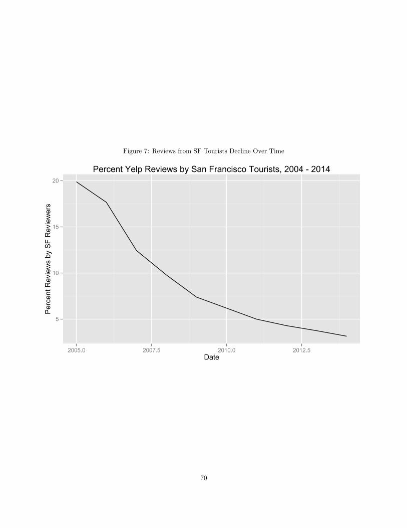
Figure 7: Reviews from SF Tourists Decline Over Time

5

10

15

20

2005.0 2007.5 2010.0 2012.5Date

Per

cent

Rev

iew

s by

SF

Rev

iew

ers

Percent Yelp Reviews by San Francisco Tourists, 2004 - 2014

70

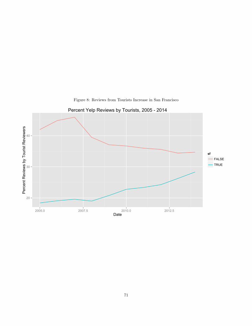
Figure 8: Reviews from Tourists Increase in San Francisco

20

30

40

2005.0 2007.5 2010.0 2012.5Date

Per

cent

Rev

iew

s by

Tou

rist R

evie

wer

s

sfFALSE

TRUE

Percent Yelp Reviews by Tourists, 2005 - 2014

71

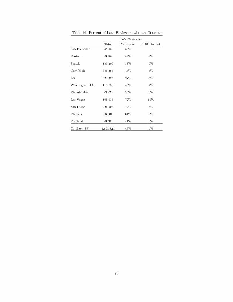
Table 16: Percent of Late Reviewers who are Tourists

Late Reviewers

Total % Tourist % SF Tourist

San Francisco 348,955 35% –

Boston 93,454 44% 4%

Seattle 135,209 38% 6%

New York 385,385 45% 5%

LA 327,395 27% 5%

Washington D.C. 118,886 48% 4%

Philadelphia 83,220 56% 3%

Las Vegas 165,035 72% 10%

San Diego 226,503 42% 6%

Phoenix 66,331 31% 3%

Portland 90,406 41% 6%

Total ex. SF 1,691,824 43% 5%

72

We find evidence consistent with hypothesis 6.2 that tourism volume is correlated with the magnitude of

spillovers. Tables 17 and 18 show that an increase of 100 flights from city i to city j in a month is correlated

with an increase of approximately 15 monthly tourist reviews. In other words, cities that have more tourist

traffic between them also have a greater magnitude of spillovers.

This relationship can also be seen anecdotally in Figures 19 and 20 in the Appendix, which show reviews of

restaurants in Seattle and Boston, respectively, generated by tourists from the top five cities of tourist origin

in each destination city. Not surprisingly, most of the spillovers are generated by tourists from geographically

proximate cities. For example, the top city of origin for tourists in Seattle is San Francisco, while the top

city of origin for tourists in Boston is New York.

73

Table 17: Cross-sectional Regression of Reviews on Flights

Dependent variable:

Reviews by Tourists from Origin City

Flights from Origin City 0.151∗∗∗

(0.008)

Observations 654R2 0.333Adjusted R2 0.332Residual Std. Error 3,723.189 (df = 652)F Statistic 325.845∗∗∗ (df = 1; 652)

Note: ∗p<0.1; ∗∗p<0.05; ∗∗∗p<0.01

Table 18: Fixed Effects Regression of Reviews on Flights

Dependent variable:

Reviews by Tourists from Origin City

Flights from Origin City 0.148∗∗∗

(0.002)

Year-month fixed effect Y

Destination city fixed effect Y

Observations 25,701R2 0.224Adjusted R2 0.221Residual Std. Error 77.474 (df = 25606)F Statistic 78.764∗∗∗ (df = 94; 25606)

Note: ∗p<0.1; ∗∗p<0.05; ∗∗∗p<0.01

74

Our findings are mixed for hypothesis 6.3. Table 19 shows there is a strong positive correlation between

early tourist reviews and future total reviews: an additional tourist review in period 1 is correlated with

approximately 22 additional reviews in period 2. Tables 20 and 21 show that this correlation is stronger for

future tourist reviews than future local reviews: an additional tourist review in period 1 is correlated with

approximately 9 local reviews versus 13 tourist reviews in period 2.

Surprisingly, there does not appear to be a positive correlation between early local reviews and future

total reviews, once accounting for early tourist reviews. In fact, an additional local review in period 1

correlates with 2 fewer tourist reviews in period 2, though it correlates with 1.4 additional local reviews in

period 2. Moreover, early local reviews are less predictive of future local reviews than early tourist reviews.

Multiple factors may be driving these results. First, and the most plausible, is that restaurants which

receive more tourist reviews in period 1 are inherently different from restaurants which receive more local

reviews in period 2. For example, tourists are more likely to patronize and review renowned restaurants than

unknown restaurants. The coefficients in column 1 of Tables 19, 20, and 21 are not therefore interpretable

as a network effect.

We ran a robustness test which tried to remove some of the omitted variable bias by controlling for the

restaurant’s average rating, a proxy for restaurant quality. We find that controlling for average rating does

not meaningfully change the coefficient. These results thus suggest that at least part of the correlation may

be driven by a causal mechanism whereby early tourist reviews drive future reviews. Further research must

be conducted to fully separate restaurant-level unobservables from a causal relationship between current and

future reviews.

75

Table 19: Effect of Early Reviews on Late Reviews

Dependent variable:

Total Reviews, Period 2

(1) (2)

Tourist Reviews, Period 1 21.579∗∗∗ 21.525∗∗∗

(0.217) (0.214)

Local Reviews, Period 2 −0.589∗∗∗ −0.620∗∗∗

(0.076) (0.075)

Avg Rating 57.095∗∗∗

(1.719)

Constant 90.650∗∗∗ −110.930∗∗∗

(1.125) (6.170)

Observations 45,841 45,841R2 0.330 0.346Adjusted R2 0.330 0.346Residual Std. Error 228.378 (df = 45838) 225.680 (df = 45837)F Statistic 11,280.820∗∗∗ (df = 2; 45838) 8,069.203∗∗∗ (df = 3; 45837)

Note: ∗p<0.1; ∗∗p<0.05; ∗∗∗p<0.01

76

Table 20: Effect of Early Reviews on Late Local Reviews

Dependent variable:

Local Reviews, Period 2

(1) (2)

Tourist Reviews, Period 1 8.697∗∗∗ 8.661∗∗∗

(0.140) (0.138)

Local Reviews, Period 1 1.432∗∗∗ 1.411∗∗∗

(0.049) (0.048)

Avg Rating 38.652∗∗∗

(1.108)

Constant 65.153∗∗∗ −71.314∗∗∗

(0.726) (3.976)

Observations 45,841 45,841R2 0.299 0.317Adjusted R2 0.299 0.317Residual Std. Error 147.341 (df = 45838) 145.423 (df = 45837)F Statistic 9,774.968∗∗∗ (df = 2; 45838) 7,095.605∗∗∗ (df = 3; 45837)

Note: ∗p<0.1; ∗∗p<0.05; ∗∗∗p<0.01

77

Table 21: Effect of Early Reviews on Late Tourist Reviews

Dependent variable:

Tourist Reviews, Period 2

(1) (2)

Tourist Reviews, Period 1 12.882∗∗∗ 12.864∗∗∗

(0.097) (0.096)

Local Reviews, Period 1 −2.021∗∗∗ −2.031∗∗∗

(0.034) (0.033)

Avg Rating 18.442∗∗∗

(0.769)

Constant 25.497∗∗∗ −39.616∗∗∗

(0.500) (2.759)

Observations 45,841 45,841R2 0.333 0.342Adjusted R2 0.333 0.342Residual Std. Error 101.539 (df = 45838) 100.908 (df = 45837)F Statistic 11,462.760∗∗∗ (df = 2; 45838) 7,929.614∗∗∗ (df = 3; 45837)

Note: ∗p<0.1; ∗∗p<0.05; ∗∗∗p<0.01

78

6.5 Discussion

Yelp is an example of a digital good that employed a lean entry strategy to grow and displace incumbent

goods in the market. Despite the presence of competitors such as YellowPages and CitySearch, Yelp focused

most of its marketing efforts on driving adoption in San Francisco during its early growth period from

January 2005 to March 2007.

This strategy was effective in large part due to spillover effects which drove user-generated content growth

in most other cities outside San Francisco. Approximately 25% of early content in cities outside of Yelp’s San

Francisco headquarters was produced by tourists from San Francisco, and an additional 19% was produced

by tourists from other cities. Spillovers are stronger between cities with high tourist traffic; we find that for

every 100 flights between two cities, tourists from the origin city leave on average 15 reviews for restaurants

in the destination city.

Though the percentage of content from spillovers has since declined in most cities due to rapid adoption

by local producers, their importance is magnified by a strong positive correlation between a restaurant’s

early spillover content and future total content. Restaurants that receive more early reviews by tourists tend

to receive more reviews in a later period by both tourists and locals. Surprisingly, the same is not true of

restaurants that receive more early reviews by locals. These findings merit further research to test for the

existence of network effects and measure its impact in driving Yelp’s growth.

We believe our research has relevance to scholars of user-generated content (UGC) and knowledge

spillovers. As far as we are aware, ours is one of the first papers to quantify knowledge spillovers as a

function of tourism volume in the context of user-generated content production. We show that spillovers for

digital goods are often directly measurable, and thus circumvent the challenge of identification experienced

by most of the prior literature.

Our research also provides insights for practitioners. Technology companies often base their choice of

which markets to enter on demographic variables such as population, income levels, and internet penetration.

For example, Yelp prefers to enter new cities where it predicts high levels of adoption by the local population.

Yet our results suggest that spillovers may be even more important than characteristics of the local population

for driving early content growth. A firm might thus prioritize entering cities which receive a high volume

of spillovers from cities where its product is currently popular, or cities which may drive a high volume of

spillovers to new markets of interest.

79

7 Summary and Conclusion

I began my thesis with a puzzle: why are new network goods more likely to succeed in some markets than

others? I showed, via a formal model, that since the strength of a market’s barriers-to-entry varies according

to its network structure, the likelihood of success depends on features of the network good and market

themselves. While markets for transaction-driven goods may fit the conventional wisdom that incumbents

are difficult to displace, markets for socially-driven goods may actually be fertile ground for entry and growth

of newcomers.

The theory of lean entry, corroborating classic theories of network effects, says firms need to seed more

than half of the market to grow in a complete or bipartite network. We saw this manifest in markets for

exchange-traded products, where the failure of entrant products to build adequate liquidity may be a primary

driver of first mover advantage. Due to the massive scale needed to enter, assets under management (a proxy

for investor demand) of most late entrants remains low, despite investments in marketing, lower pricing, and

usually comparable distribution channels.

The theory also says that, in contrast with classic theories of network effects, seeding relatively few

early adopters can lead to discontinuous growth in markets with diffusive network structure. We saw this

manifest for digital content aggregator Yelp, which employed a lean entry strategy of focusing on seeding

early adopters within San Francisco but later exploited a spillover effect to grow.

Finally, the theory shows which networks are most likely to be diffusive: those with cohesive subsets of

consumers that also contain boundary spanners. We saw in the case of Yelp that local users within cities are

cohesive while tourists between cities act as boundary spanners. Though tourists drove a negligible fraction

of Yelp’s later growth, their influence on Yelp’s early growth was potentially magnified by a network effect

whereby early spillover content drove later content production.

From a prescriptive point of view, producers of network goods should tailor their entry and growth

strategies to fit features of the market and the good they are trying to sell. They should pay close attention

to how network effects are generated, in particular whether the network good is transaction-driven or socially-

driven. For example, strategies which proved successful for Vanguard’s exchange-traded products included

bundling with an existing class of investment products, which helped seed liquidity critical for entry. For

socially-driven network goods such as Yelp, such initial scale was neither necessary nor sufficient for growth.

The final insight for practitioners is that network effects alone do not guarantee a competitive advantage.

Because barriers-to-entry in network markets are weaker than previously thought, paying high acquisition

prices for socially-driven network goods may not be justified by the theory of network effects. To recall a

80

historical example, AOL acquired communications technology ICQ in 1998 for 400M, a record price at the

time. Network effects generated by a large installed base of Instant Messenger and ICQ users seemed to

give AOL a massive advantage against competitors in this market. Less than 10 years after the acquisition,

AOL’s Instant Messenger was displaced by new digital communications technologies such as gChat, Skype,

and Facebook.

81

References

[1] Sean parker on why myspace lost to facebook, http://techcrunch.com/2011/06/28/sean-parker-on-why-

myspace-lost-to-facebook/, Accessed: 2014-07-12.

[2] Howard Aldrich and Diane Herker, Boundary spanning roles and organization structure, Academy of

Management Review 2 (1977), no. 2, 217–230.

[3] Franklin Allen and Douglas M Gale, Financial innovation and risk sharing, MIT press, 1994.

[4] Sinan Aral, Lev Muchnik, and Arun Sundararajan, Engineering social contagions: Optimal network

seeding in the presence of homophily, Network Science 1 (2013), no. 02, 125–153.

[5] Sinan Aral and Dylan Walker, Identifying influential and susceptible members of social networks, Science

337 (2012), no. 6092, 337–341.

[6] Kenneth J Arrow, The economic implications of learning by doing, The review of economic studies

(1962), 155–173.

[7] C. Ballester, A. Calvo-Armengol, and Y. Zenou, Who’s who in networks. wanted: the key player, Econo-

metrica 74 (2006), no. 5, 1403–1417.

[8] Arup Banerji and Bhaskar Dutta, Local network externalities and market segmentation, International

Journal of Industrial Organization 27 (2009), no. 5, 605–614.

[9] Ernst R Berndt, Linda Bui, David R Reiley, and Glen L Urban, Information, marketing, and pricing

in the us antiulcer drug market, The American Economic Review 85 (1995), no. 2, 100–105.

[10] Luis MB Cabral, On the adoption of innovations with networkexternalities, Mathematical Social Sciences

19 (1990), no. 3, 299–308.

[11] I. Dierickx and K. Cool, Asset stock accumulation and sustainability of competitive advantage, Manage-

ment Science 35 (1989), no. 12, 1504–1511.

[12] Darrell Duffie and Rohit Rahi, Financial market innovation and security design: An introduction,

Journal of Economic Theory 65 (1995), no. 1, 1–42.

[13] Thomas Eisenmann, Geoffrey Parker, and Marshall Van Alstyne, Platform envelopment, Strategic Man-

agement Journal 32 (2011), no. 12, 1270–1285.

82

[14] David S Evans and Richard Schmalensee, Failure to launch: Critical mass in platform businesses, Review

of Network Economics 9 (2011), no. 4.

[15] J. Farrel and G. Saloner, Installed base and compatibility: Innovation, product preannouncements, and

predation, American Economic Review 76 (1986), no. 5, 940–955.

[16] Joseph Farrell and Paul Klemperer, Coordination and lock-in: Competition with switching costs and

network effects, Handbook of industrial organization 3 (2007), 1967–2072.

[17] Joseph Farrell and Garth Saloner, Installed base and compatibility: Innovation, product preannounce-

ments, and predation, The American economic review (1986), 940–955.

[18] Joseph Farrell and Carl Shapiro, Dynamic competition with switching costs, The RAND Journal of

Economics (1988), 123–137.

[19] D. Fudenberg and J. Tirole, Pricing a network good to deter entry, Journal of Industrial Economics 48

(2000), no. 4, 373–390.

[20] A. Galeotti and S. Goyal, Influencing the influencers: a theory of strategic diffusion, RAND Journal of

Economics 40 (2009), no. 3, 509–532.

[21] Peter N Golder and Gerard J Tellis, Pioneer advantage: marketing logic or marketing legend?, Journal

of marketing Research (1993), 158–170.

[22] Richard Hall, A framework linking intangible resources and capabilities to sustainable competitive ad-

vantage, Strategic management journal 14 (1993), no. 8, 607–618.

[23] Oliver Hinz, Bernd Skiera, Christian Barrot, and Jan U Becker, Seeding strategies for viral marketing:

an empirical comparison, Journal of Marketing 75 (2011), no. 6, 55–71.

[24] Ali Hortacsu and Chad Syverson, Product differentiation, search costs, and competition in the mutual

fund industry: A case study of s&p 500 index funds, The Quarterly Journal of Economics 119 (2004),

no. 2, 403–456.

[25] Mark A Hurwitz and Richard E Caves, Persuasion or information? promotion and the shares of brand

name and generic pharmaceuticals, Journal of Law and Economics 31 (1988), no. 2, 299–320.

[26] M. Jackson, Social and economic networks, Princeton University Press, 2008.

83

[27] Boyan Jovanovic and Saul Lach, Entry, exit, and diffusion with learning by doing, Tech. report, 1988.

[28] M. Katz and C. Shapiro, Network externalities, competition, and compatibility, American Economic

Review 75 (1985), no. 3, 424–440.

[29] , Technology adoption in the presence of network externalities, Journal of Political Economy 94

(1986), no. 4, 822–841.

[30] , Systems competition and network effects, Journal of Economic Perspectives 8 (1994), no. 2,

93–115.

[31] Michael L Katz and Carl Shapiro, Product introduction with network externalities, The Journal of

Industrial Economics (1992), 55–83.

[32] Paul Klemperer, Markets with consumer switching costs, The Quarterly Journal of Economics 102

(1987), no. 2, 375–394.

[33] Eocman Lee, Jeho Lee, and Jongseok Lee, Reconsideration of the winner take all hypothesis: complex

networks and local bias, Management Science 52 (2006), no. 12, 1838–1848.

[34] Jure Leskovec and Andrej Krevl, SNAP Datasets: Stanford large network dataset collection, http:

//snap.stanford.edu/data, June 2014.

[35] Marvin B Lieberman and David B Montgomery, First-mover advantages, Strategic management journal

9 (1988), no. S1, 41–58.

[36] S. Morris, Contagion, Review of Economic Studies 67 (2000), no. 1, 57–78.

[37] Christine Oliver, Sustainable competitive advantage: Combining institutional and resource-based views,

Strategic management journal 18 (1997), no. 9, 697–713.

[38] Richard Reed and Robert J DeFillippi, Causal ambiguity, barriers to imitation, and sustainable com-

petitive advantage, Academy of management review 15 (1990), no. 1, 88–102.

[39] William T Robinson, Gurumurthy Kalyanaram, and Glen L Urban, First-mover advantages from pio-

neering new markets: A survey of empirical evidence, Review of Industrial Organization 9 (1994), no. 1,

1–23.

[40] Richard Schmalensee, Entry deterrence in the ready-to-eat breakfast cereal industry, The Bell Journal of

Economics (1978), 305–327.

84

[41] Avner Shaked and John Sutton, Product differentiation and industrial structure, The Journal of Indus-

trial Economics (1987), 131–146.

[42] A Michael Spence, The learning curve and competition, The Bell Journal of Economics (1981), 49–70.

[43] Dale O Stahl, Oligopolistic pricing with sequential consumer search, The American Economic Review

(1989), 700–712.

[44] A. Sundararajan, Local network effects and complex network structure, B.E. Journal of Theoretical

Economics 7 (2007), no. 1, Article 46.

[45] Peter Tufano, Financial innovation and first-mover advantages, Journal of Financial Economics 25

(1989), no. 2, 213–240.

[46] , Financial innovation, Handbook of the Economics of Finance 1 (2003), 307–335.

[47] Pieter A VanderWerf and John F Mahon, Meta-analysis of the impact of research methods on findings

of first-mover advantage, Management Science 43 (1997), no. 11, 1510–1519.

[48] H. Varian and C. Shapiro, Information rules: a strategic guide to the network economy, Harvard Business

Review Press, 1998.

[49] Feng Zhu and Marco Iansiti, Entry into platform-based markets, Strategic Management Journal 33

(2012), no. 1, 88–106.

85

8 Appendix

8.1 Lean Entry in Network Markets

8.1.1 Proofs

Lemma 8.1. Diffusion reaches a unique equilibrium φ(x) ∈ X∗ from any initial state of adoption x ∈ X.

Moreover, φ(x) is weakly lower than the equilibrium reached by any locally rational diffusion process from x.

Proof. 8.1 Take the diffusion process with starting state x1 = (0, . . . , 0). We have proved that this process

reaches an equilibrium x∗. That equilibrium is an equilibrium for the model of demand, since for every i,

bi(x∗) = xi.

For complete networks, the set X∗ = {“all adopt,” “none adopt”} is analogous to the familiar fulfilled

expectations equilibria of Katz and Shapiro (1985), since network utilities corresponding to a complete

network are identical to network utilities in a reduced-form model of network effects.

Observe since L(i) = N for all i ∈ N in a complete network, value of the network must be the same for

all agents. Thus we can translate our framework into the Katz and Shapiro framework by assuming a price

p (in our case zero) and random distribution of θ over [0, 1] (in our case a null distribution where θ equals

a constant), by normalizing α = 1n , and by letting q∗ =

∑i∈L(i) x

∗i = ||x∗||. Define a marginal consumer of

type θ̂ as a function of α, n, p: let θ̂ be the lowest type such that θ̂ − p+ αq∗ ≥ 0. In equilibrium, all agents

with types greater than or equal to θ̂ must adopt. If we assume n is large enough for the random draw on

types to be approximately continuous, in expectation this yields 1 − θ̂ = 1 − p + αq∗ = q∗

n as the unique

fraction of the market which adopts in a fulfilled expectations equilibrium, or q∗ = n(1−p)1−αn .

We will now prove the second part of the Lemma. From an initial state x and an arbitrary locally

rational diffusion process {yτ}∞τ=1, y1 = x converging to equilibrium y∗, we will show that the diffusion

process reaches a weakly lower equilibrium than {yτ}∞τ=1.

As above, note that in the diffusion process, agents drop out until we reach a state in which everyone

who is adopting is best responding. More formally, in the diffusion process, x1 � x2 � · · · � xτ0 for some τ0,

after which there are no more agents i such that xτ0i = 1 and bi(xτ0) = 0. After that, xτ0 � xτ0+1 � xτ0+2 �

· · · � xτ∗, where xτ

∗is the equilibrium reached by the diffusion process. Note that the set of adopters in

xτ0 is self-sufficient. Let us call this set x̄.

Note that the set of adopters in x̄ is contained in the initial state: x̄ � x, and also note that any locally

rational diffusion process will retain x̄ within the set of adopters. More formally, x̄ � yτ∀τ .

86

Indeed, assume the opposite, and suppose that i is the first agent within the set of adopters in x̄ to switch

from xi = 1 to xi = 0, and that it happens on some step τ : xτi = 1, xτ+1i = 0. Then, at that step, bi(y

τ ) = 0

must be zero, which is not possible, since the set of adopters in yτ would contain all the adopters in x̄, which

means that bi(yτ ) = 1, and so we have a contradiction.

Therefore, y∗ � x̄ = xτ0 . Thus, for every i for which bi(xτ0) = 1, bi(y

∗) ≥ bi(xτ0) = 1, and so y∗ � xτ0+1.

By the same logic, that leads to y∗ � xτ0+2, and so on, we conclude that y∗ � xτ∗ .

Proof. 4.1 Let {xτ}∞τ=0 and {yτ}∞τ=0 be the two processes, with x1 = x and y1 = y. As discussed above,

in each process, adopters drop out, after which the adopter base grows, until we reach an equilibrium:

y1 � y2 � · · · � yτ0 � yτ0+1 � · · · � y∗. Note that x � y � yτ0 , and since the adopters in yτ0 are a

self-sufficient set, then by the same argument as in the proof of A4.2., xτ � yτ0 for every τ , and so x∗ � yτ0 ,

and again as above, this leads to x∗ � yτ0+1, x∗ � yτ0+2 and so on, until x∗ � y∗.

To prove D(x) ≥ D(x′) does not imply x � x′ or ||x|| ≥ ||x′||, we provide a counterexample. Consider a

network G(N,L) which consists of two disconnected subgraphs: five nodes whose links form a pentagon and

five nodes forming a complete subgraph. Let there be no links between nodes in the two subgraphs.

Assuming thresholds for adoption are t=1 for all i ∈ N , Seeding any three adopters in the pentagon leads

to demand 0, while seeding any three adopters in the complete network leads to demand 5. This concludes

the proof.

Proof. 4.2 A state x is self-sustaining if and only if for every agent i in A(x), the best response given the

status quo is to remain an adopter of the entrants good. When the status quo is y∗i = 1 ∀i ∈ N , this is

equivalent to more than half of is peers are in A(x) for every i ∈ A(x), which is the definition of 12 -cohesion.

In general, this is equivalent to more than ti of i’s peers are in A(x) for every i ∈ A(x), which by a simple

reordering of ρi >tidi

, is the definition of t-cohesion.

Proof. 4.3 First, note that in Proposition 4.2, we established that once the diffusion process has reached a

self-sustaining state, the process only takes us to weakly greater states.

We will prove the first claim of our proposition by induction. By Proposition 5.3., A(x1) is t-cohesive.

Suppose that A(xτ−1) is also t-cohesive; we will show that A(xτ ) is also t-cohesive. If xτ−1 = xτ , our claim

is obviously true. Assume xτ−1 6= xτ .

Take an agent i which joins the set of adopters on step τ , i.e. i ∈ A(xτ )\A(xτ−1). Then, bi(xτ−1) = 1,

which means that more than tidi

of their peers are in A(xτ−1), and so more than tidi

of their peers are in

87

A(xτ ) ⊃ A(xτ−1). Additionally, for every agent j ∈ A(xτ−1), more than tidi

of their peers are in A(xτ−1),

and so more than tidi

of their peers are in A(xτ ) ⊃ A(xτ−1). Thus, A(xτ ) is also t-cohesive.

Now, suppose that for some τ , there is no such i /∈ A(τ) such that more than tidi

of is peers are in A(xτ ).

This means that there is no agent which isnt currently adopting the entrants good, whose best response in

step τ would be to adopt. Therefore, the diffusion process will not add any further adopters. It will also

not remove any adopters, since A(xτ ) is t-cohesive and thus self-sustaining, and so diffusion has reached an

equilibrium.

Proof. 1 (Corollary to Prop 4.3) Suppose that for some τ , C = N\A(xτ ) is weakly (d− t)-cohesive, that is

every i has a proportion of its peers in C of at least (di − ti)/di = 1 − ti/di. In the case when the outside

option is a network good, this is equivalent to saying the proportion ρi of i’s peers in A(xτ ) is no more than

ti/di for all i ∈ C. This means there is no consumer in C whose best response is to adopt, and since A(xτ )

is self-sustaining, diffusion has reached an equilibrium.

Proof. 4.4 Suppose every consumer has already adopted a network good and we are now interested in

diffusion of an identical competing (focal) network good. Let the diffusion process be described by the

nested t-cohesive sets A1 ⊂ A2 ⊂ · · · ⊂ AT . Let the number of links between adopters in A1 be denoted

l, and let the minimum threshold for adopting a network good (versus a non-network outside option) be

denoted btc.

We will assign 2l unique labels, numbered 1 through 2l, to nodes in A1: for every node, assign as many

different labels as the number of the node’s peers in A1. We will then reassign the labels to nodes that adopt

the focal good. Eventually, every node that adopts the focal good will be assigned at least one unique label;

at least one will get bt + 1c and some others may get more than one. That will conclude our proof that

diffusion reaches a strict upper bound D̄(x) = ||x||(||x|| − 1) (subtracting btc if it is greater than zero).

Note that for each adopter of the focal good in x, we have more links connecting it to other adopters in

x than“outgoing links.” On every step of the diffusion process, the same will hold: for a node i ∈ Aj\Aj−1,

there are more links from i to nodes in Aj−1 than links from i to nodes outside of Aj−1. Using this fact, we

will assign labels along the path of diffusion using iteration.

Step 0. Begin the method of reassigning labels by having each node i in A1 “give” a label to each of its

peers outside A1. Since i has more links within A1 than without, it will retain at least one label for itself.

Also, note that every node j in A1 will have received a number of labels equal to the number of links from

j to A1.

88

Step 1. For each node i in A2\A1, reassign one label to each of its peers outside S1. Again, this means

that every node in A2\A1 will retain at least one label for itself.

In step m of our labeling method, let each node i ∈ Am\Am−1 reassign the labels to each of its peers

outside Am. Since we know that i in Am has so far received 1 label from each of its peers in Am−1, and i

adopted on the m-th step of the diffusion process, i must have strictly more neighbors in Am−1 than peers

outside of Am−1, and thus outside of Sm. This means that i will retain at least one label for itself.

We can repeat this method until we reach AT , the last step of the diffusion process. Note that for every

node in AT , there will be at least bt + 1c labels reassigned and retained by each node in AT . Every other

node will have received and retained at least one label. Since we started out with 2l labels, this concludes

the proof that diffusion reaches a strict upper bound of ||x||(||x|| − 1) adopters.

Proof. 2 We can use the same labeling method to show that networks which maximize diffusion when θ = 0

are nestedly 12 -cohesive such that each adopter is a boundary spanner between two nested sets. Maximum

diffusion from size ||x|| occurs when the network can be broken up into components A0, A1, A2, . . . , AT such

that:

1. A0 is a complete subgraph of size ||x||

2. For every s ≥ 1, the nodes of As have no links to other nodes in As, and each node i in As has exactly

1 more links to ∪s−1j=0Aj than to ∪ks+1Aj .

3. If the minimum threshold for adopting a network good (versus a non-network outside option) is at

least one, the last component Ak has exactly 1 element, with exactly bt+1c links. If the minimum threshold

is less than one, then AK can have as many elements, but each of them has one incoming links and no links

exist between nodes in Ak.

Following labeling method, note that conditions 1-3 above are necessary and sufficient to ensure exactly

|Ai| labels remain assigned to the nodes of Ai on the ith step of the diffusion. For the final step, note that

each of the nodes in Ak needs to have more than t links coming in, so each node in Ak needs to retain at

least bt+ 1c labels for itself. To minimize the number of “excess labels” in this last phase, Ak needs to have

only one node if t ≥ 1.

Proof. 4.1 Since every node is connected to every other node in a complete network, a state x is self-sustaining

only if each seeded node is connected to more than n−12 −

θ2α other seeded nodes. Note that the subgraph

defined by the nodes in A(x) is complete, and each node in it has degree ||x|| − 1. Thus for x to be self-

sustaining, it is necessary for ||x|| − 1 ≥ bn−12 −θ2αc+ 1 or equivalently ||x|| ≥ bn−12 −

θ2αc+ 2. Observe that

89

this lower bound is also sufficient for diffusion to reach demand n in one iteration, since every node in the

entire network would be connected to more than n−12 −

θ2α seeded nodes. It is the minimal scale because

x∗ = (1, 1, . . . , 1) is the lowest equilibrium with nonzero demand.

The seed state bn−12 −θ2αc + 2 is bounded above by a scalar multiple of n as n → ∞, which completes

our proof that the entrant must seed more than half the market to enter a complete network.

I now show that an entrant must seed more than half of a bipartite network in order to enter the market.

Suppose we have a bipartite graph with N1 sellers on one side of the network and N2 buyers on the other

side. Let S0 6= ∅ be a self-sustaining set of adopters; without loss of generality, assume that S0 ∩ N1 6= ∅.

Let x be a seller in S0 ∩ N1. Since at least half of x’s peers must be in S0 in order for x’s adoption to be

self-sustaining, and x is linked to all buyers in N2 and no other consumers, it must be that |S0∩N2| > |N2|/2.

Similarly, consider a buyer on the other side: y ∈ S0 ∩N2. Since y is linked to none all sellers in N1 and

no other consumers, it must be that |S0 ∩N1| > |N1|/2 in order for S0 to be self-sustaining. This argument

shows that |S0| = |S0 ∩N1|+ |S0 ∩N2| > |N1|/2 + |N2|/2 = |N |/2, in other words at least half the market

must adopt the entrant’s good for its presence in the market to be sustainable.

Proof. 4.2 This follows directly from Proposition 4.4. In the optimally diffusive network described there, DP

reaches at least D(x) = ||x||(||x|| − 1) + θαγn adopters from x. This is true for arbitrarily large ||x||, so set

D(x) = n for an arbitrarily large n and solve for x. DP reaches demand n from ||x|| = m early adopters,

where m is the smallest integer for which m(m− 1) + θαγn ≥ n. By definition, the minimal scale needed to

enter cannot be more than m.

Since m is bounded above by a scalar multiple of√n as n→∞, this completes our proof.

Proof. 4.5 This follows from 4.2 and 4.1, since in a complete network, minimal scale to entry grows in the

order of O(n), and in an optimally diffusive network it grows in the order of at most O(√n) .

Proof. 4.3 Take an arbitrary number m. We will show that there exists an optimal network of size m(m−1)

with average degree m.

Denote the nodes a1, . . . , am; b1, . . . , bm(m−3)/2; c1, . . . , cm(m−1)/2. Let the nodes be connected as follows:

{ai} is an m-clique;

b1 is connected to m of the ai-s; b2 is connected to m− 1 of the ai-s, and so on, until bm which is connected

to 1 of the ai-s.

bm+1 through bm(m−3)/2 is connected to 1 of the ai-s each, in such a way that every ai has exactly m − 2

edges connecting it with some of the bi-s.

90

bi and bj are connected iff |i− j| ≤ m− 1 for every i and j.

bm(m−5)/2+2 is connected to 1 ci; bm(m−5)/2+3 is connected to 2 ci-s, and so on until bm(m−3)/2 which is

connected to m− 1 of the ci-s, in such a way that each ci is connected to exactly one of the bi-s.

Note that if the firm seeds {ai}mi=1, that is a self-sustaining state because each ai will have m− 1 edges

to other ais and only m − 2 edges to non-adopters. On each iteration of the diffusion process the bi-s will

adopt in order starting with b1, b2, . . .: For example, on the first round of diffusion, b1 is connected to m

adopters (the ai-s) and m − 1 non-adopters, b2 through bm. On the next iteration, b2 will be connected to

m adopters (the ai-s it is connected to, and b1) and m− 1 non-adopters again.

This continues until bm. Now for bm+1 through bm(m−3)/2, again, on each round, take the node with

lowest index which has not yet adopted, and note that it is then connected to m adopters (m− 1 of the bi-s

and 1 of the ais) and m− 1 non-adopters (bi-s and in some cases, a number of ci-s).

Finally, by the time all the bi-s have adopted, each ci will have exactly 1 adopting neighbor and 0 non-

adopting, so they will all adopt as well.

Thus, we have provided an example with n = m+m(m− 3)/2 +m(m− 1)/2 = m(m− 1) nodes which

diffuses from initial seed size m. Let us count the total number of edges:

m(m− 1)/2 from ai to aj ;

m(m− 2) from ai to bj ; (s− 1) + (s− 2) + · · ·+ (s−m+ 1) from bi to bj , where s = m(m− 3/2);

m(m− 1)/2 from bi to cj , or a total of

m(m− 1)/2 +m(m− 2) + ((m− 1)s−m(m− 1)/2) +m(m− 1)/2 =

m(m− 1)/2 +m(m− 2) + (m− 1)m(m− 3)/2 =

m2 −m+ 2m2 − 4m+m3 − 4m2 + 3m

2=

m3 −m2 − 2m

2=m(m+ 1)(m− 2)

2

Since the total sum of nodes’ degrees is twice the number of edges, this means that the average degree in

91

our network is m(m+1)(m−2)m(m−1) = (m+1)(m−2)

m−1 >√n.

Proof. 4.6 Recall that πL(n) = n(θ + αnk)− c(m) where m2 −m = (1− θαγ)n;

π∗C(n) = n(θ + α(n− 1))− c(bn−12 −θ2αc+ 2);

π∗B(n) = nθ − 1.

Suppose ||x||2 < c(||x||) < ||x||2(k+1). We will first show that πL(n) − π∗C(n) > 0 as n → ∞. Since

c(||x||) > ||x||2 asymptotically, the term with highest polynomial degree in πL(n) − π∗C(n) is cC(n) =

c(bn−12 −θ2αc+2). Observe that cC(n)→ +∞ as n→∞. Thus, there exists n0 such that πL(n)−π∗C(n) > 0

for all n > n0. And since c(||x||) < ||x||2(k+1), πL(n) = π∗L(n).

We will now show that πL(n) − π∗B(n) > 0 as n → ∞. The term with highest polynomial degree in

πL(n)− π∗B(n) is αnk+1. Since that term grows to +∞, there exists n1 such that πL(n)− π∗B(n) > 0 for all

n > n1. It follows that π∗L(n)− π∗B(n) > πL(n)− π∗B(n) > 0 for all n > n1.

We have shown that for sufficiently large n > max(n0, n1), the firm achieves greater profit in the optimally

diffusive network than in both a complete and empty network.

Proof. 4.7 Let us denote with x′∗ and x∗ the entrant’s demand equilibrium given adoption of the incumbent’s

good y∗ and y∗ respectively. We will prove that x∗ � x∗. Let {xτ} and {xτ} be the diffusion process that

reach those equilibria, and let us also denote with {yτ} and {yτ} the respective incumbent’s adopters in each

step of diffusion.

Suppose that the initial state x = x1 = x1 is such that every agent who adopts is also already best-

responding. Then, each diffusion process will only add new agents to the set of adopters of the entrants

good, and it will do so in a way that the set of adopters remains self-sustaining. On the other hand, the set

of adopters of the incumbents good will only be reduced during the diffusion process.

Note that if on a given step τ , xτ � xτ and yτ � yτ , then the same is true for step τ + 1. Indeed, take

an agent i that switched on step τ + 1 from not adopting the entrants good, to adopting it. Then, the best

response for i given adopter set xτ and status quo yτ is to adopt the entrants good. Thus, the best response

for i given adopter set xτ � xτ and status quo yτ � yτ will also be to adopt the entrants good. Thus,

xτ+1 � xτ+1. Analogously, yτ+1 � yτ+1 (since every agent j who dropped out of yτ also dropped out of

yτ ), and so the equilibrium reached by {xτ} is weakly lower than the one reached by {xτ}.

Note that the above claim is true if the two diffusion processs start off from different initial self-sustaining

92

states of adoption: that is, we only need x1 � x1, not x1 = x1, and the above argument still holds.

Going back to the general case, in the first phase of the two diffusion processs (when agents drop the

entrants good), the adopter bases reduce to self-sustaining sets xτ0 and xτ0 . We will now show that xτ0 � xτ0

and yτ0 � yτ0 , and combined with the above argument, this will conclude our proof. Note that since xτ0 is

self-sustaining given a status quo yτ0 , and since y1 � y1 � y2 � · · · � yτ0 , xτ0 is both contained in x1, and

self-sustaining given status quo y1. We will show by induction that for every step τ , xτ � xτ0 and yτ � yτ0 .

Suppose the opposite: let τ+1 be the first step for which the above is not true. There are two possibilities.

First, there is an agent i for whom xτ0i = 1 and xτi = 1 but xτ+1i = 0. Since xτ � xτ0 and yτ � yτ0 , that is

not possible, since then xτ+1i 6= bi(x

τ ).

Second, it could be that there is an agent i for whom yτ0i = 0 and yτi = 0 but yτ+1i = 1. Again, since

xτ � xτ0 and yτ � yτ0 , the best response for i given entrant adopter set xτ and status quo yτ cannot be

more favorable for the incumbent than xτ0 and yτ0 , and so we have a contradiction again, which completes

our proof.

93

8.2 First Mover Advantage of Exchange-Traded Products

94

Figure 9: ETP Construction

95

Figure 10: ETP Industry Growth

96

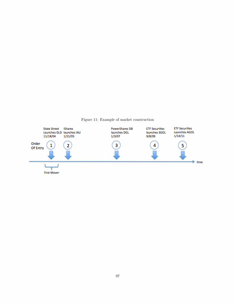
Figure 11: Example of market construction

97

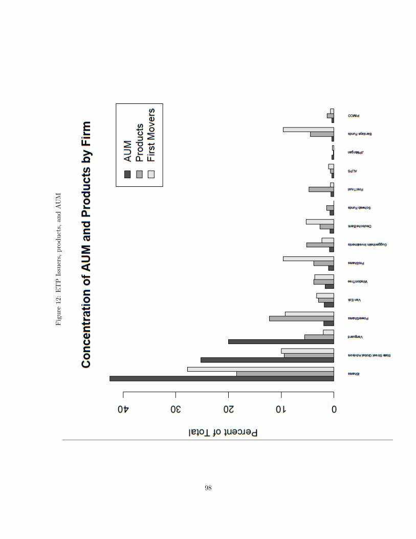
Fig

ure

12:

ET

PIs

suer

s,p

rod

uct

s,an

dA

UM

98

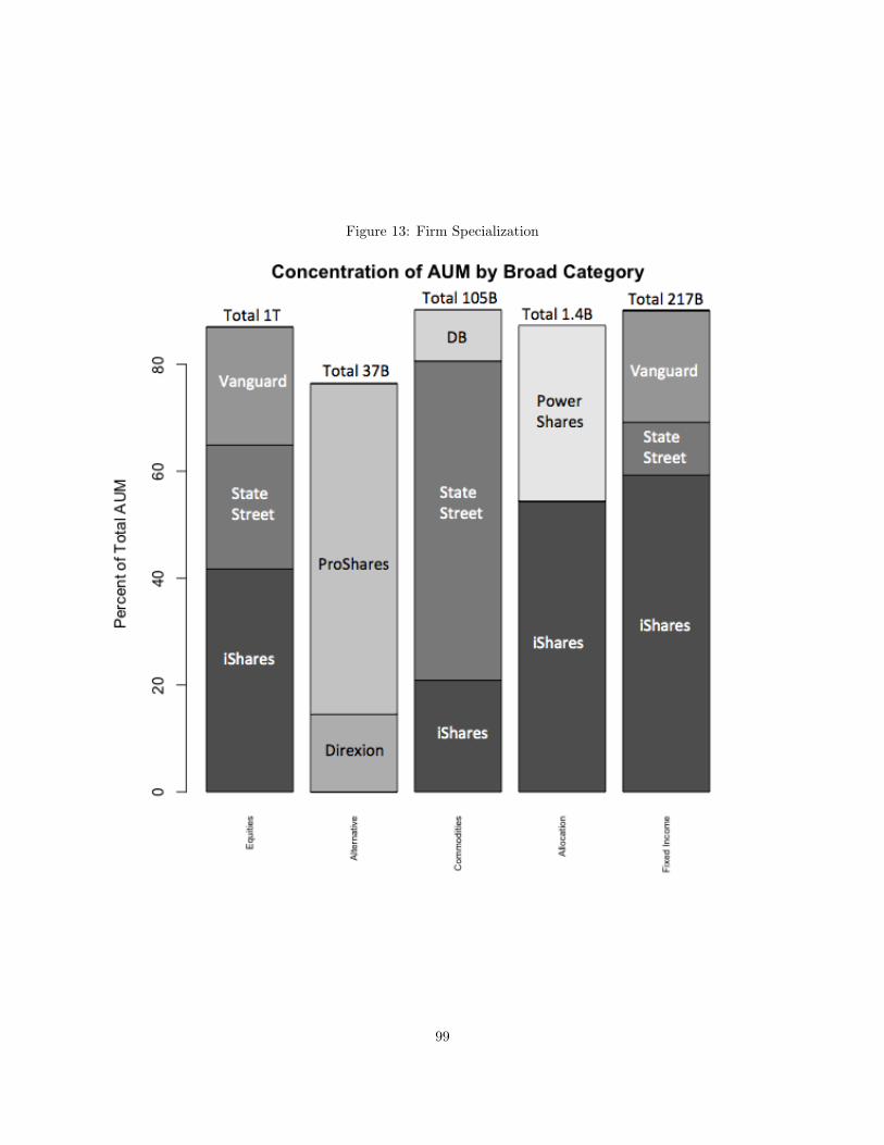
Figure 13: Firm Specialization

99

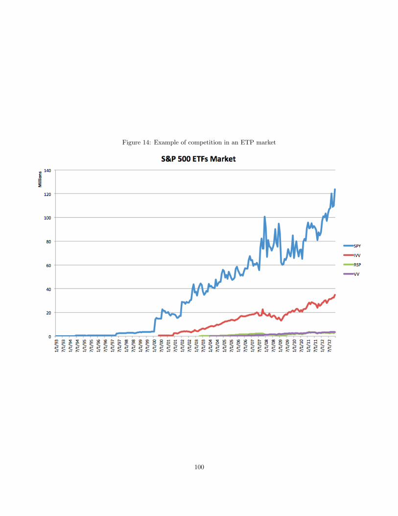
Figure 14: Example of competition in an ETP market

100

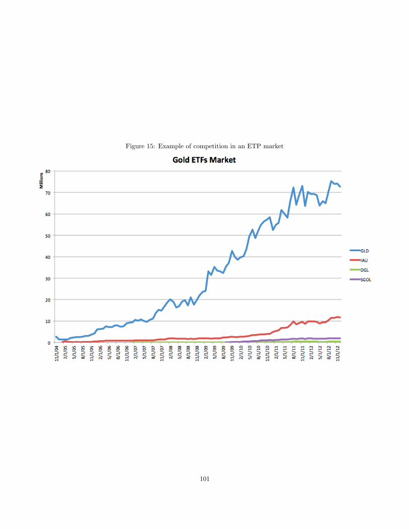
Figure 15: Example of competition in an ETP market

101

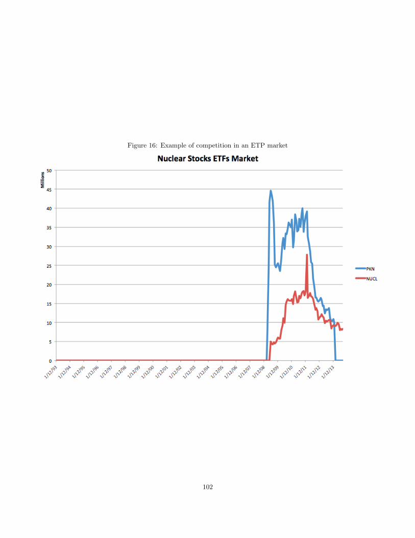
Figure 16: Example of competition in an ETP market

102

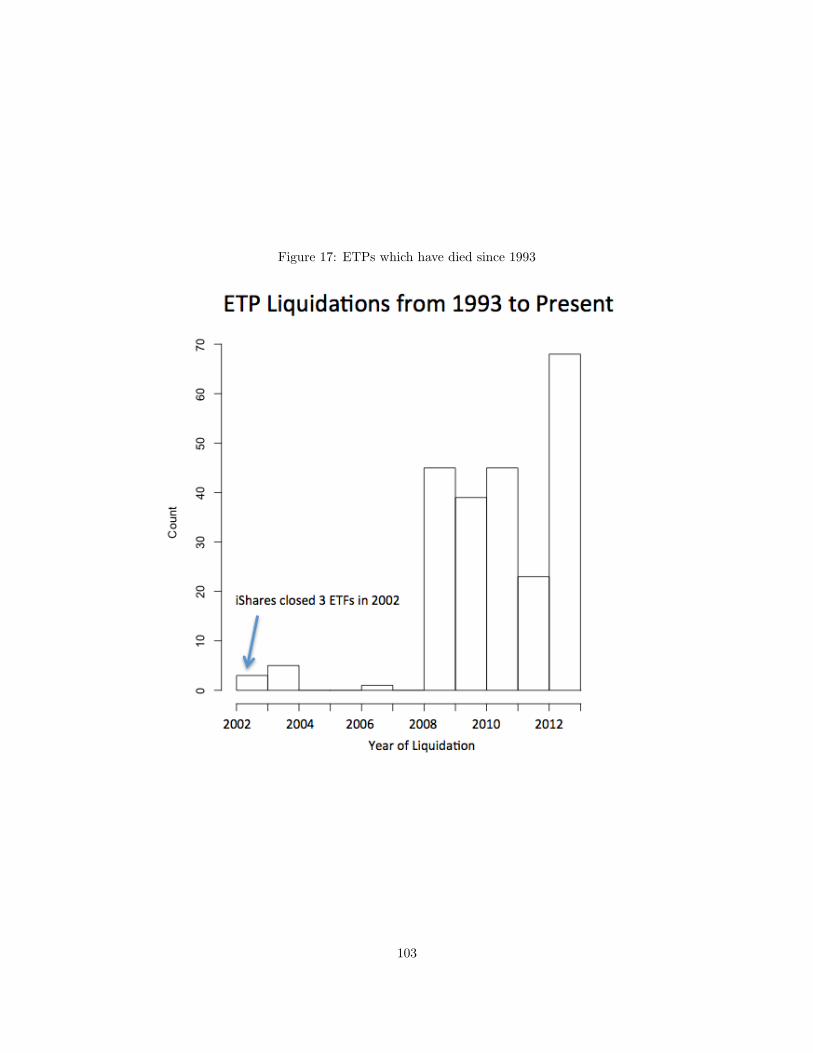
Figure 17: ETPs which have died since 1993

103

Table 22: Correlation Table for AUM Difference between 1st and 2nd Mover

Correlated Variable log AUM Difference

Market Size 0.062Market Inception Year −0.268

Days before 2nd mover Entry 0.265First Mover initial capital 0.072First Mover 6 month AUM 0.140Second mover initial capital 0.036Second mover 6 month AUM 0.034

104

8.3 Growing Digital Content: the Case of Yelp.com

105

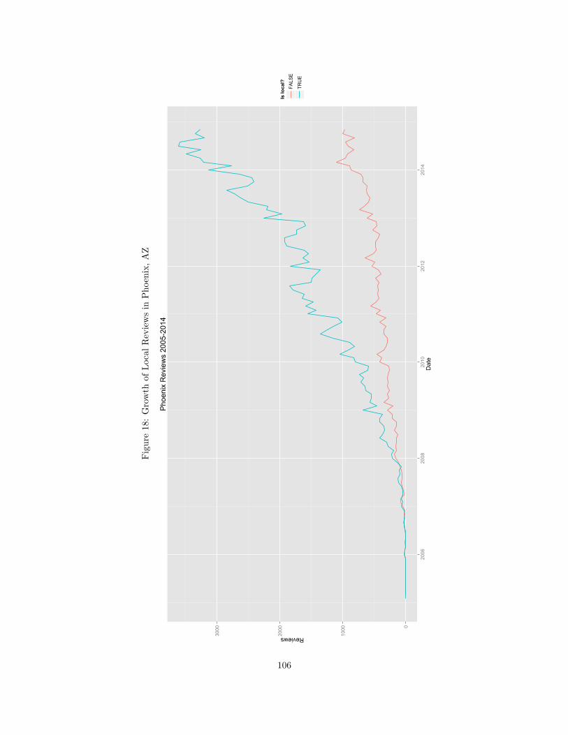
Fig

ure

18:

Gro

wth

of

Loca

lR

evie

ws

inP

hoen

ix,

AZ

0

1000

2000

3000

2006

2008

2010

2012

2014

Date

Reviews

Is lo

cal?

FALS

E

TRUE

Pho

enix

Rev

iew

s 20

05-2

014

106

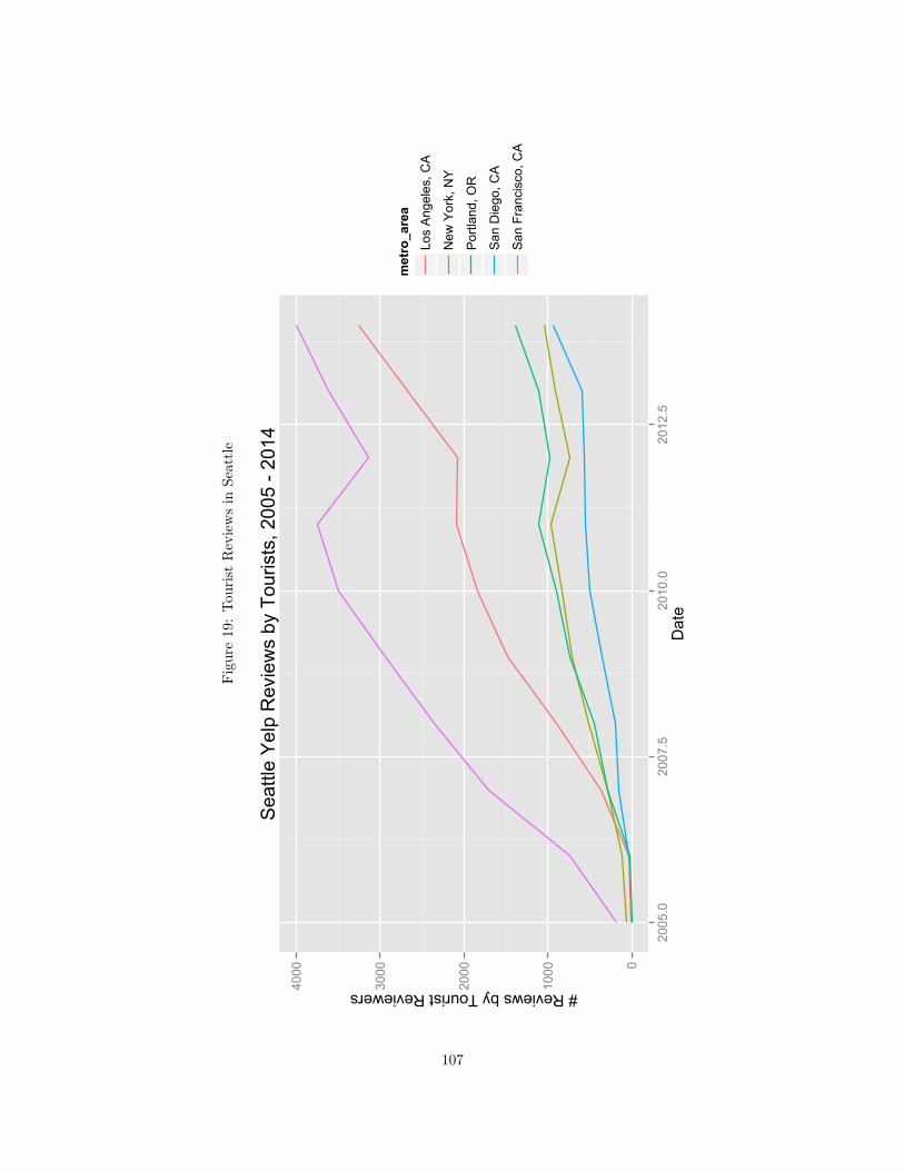
Fig

ure

19:

Tou

rist

Rev

iew

sin

Sea

ttle

0

1000

2000

3000

4000

2005

.020

07.5

2010

.020

12.5

Date

# Reviews by Tourist Reviewers

metro_a

rea

Los

Ang

eles

, CA

New

Yor

k, N

Y

Por

tland

, OR

San

Die

go, C

A

San

Fra

ncis

co, C

A

Sea

ttle

Yel

p R

evie

ws

by T

ouris

ts, 2

005

- 201

4

107

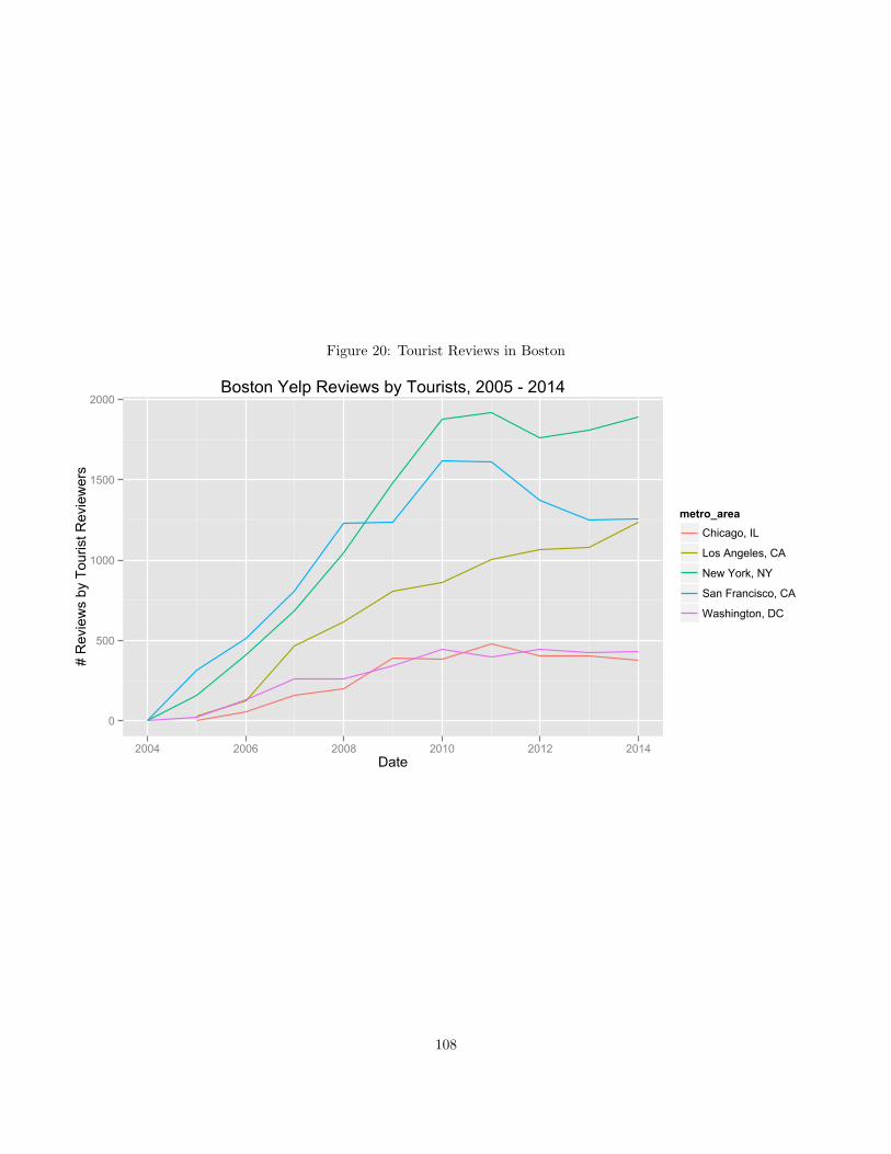
Figure 20: Tourist Reviews in Boston

0

500

1000

1500

2000

2004 2006 2008 2010 2012 2014Date

# R

evie

ws

by T

ouris

t Rev

iew

ers

metro_areaChicago, IL

Los Angeles, CA

New York, NY

San Francisco, CA

Washington, DC

Boston Yelp Reviews by Tourists, 2005 - 2014

108