strategies for managing cool thermal energy storage with

Strategies for Managing Cool Thermal Energy Storage with

Day-ahead PV and Building Load Forecasting at a District Level

Abdullah Alfadda

Dissertation submitted to the faculty of the Virginia Polytechnic Institute and State

University in partial fulfillment of the requirements for the degree of

Doctor of Philosophy

in

Computer Engineering

Saifur Rahman, Chair

Amos L. Abbott

Manisa Pipattanasomporn

Naren Ramakrishnan

Virgilio A. Centeno

August 13, 2019

Blacksburg, VA

Keywords: Machine Learning, Artificial Intelligence, Smart Grids, Solar Forecasting,

Energy Storage

Strategies for Managing Cool Thermal Energy Storage with Day-ahead PV and Building Load Forecasting at a District Level

Abdullah Alfadda

Abstract

In hot climate areas, the electrical load in a building spikes, but not by the

same amount daily due to various conditions. In order to cover the hottest day of

the year, large cooling systems are installed, but are not fully utilized during all hot

summer days. As a result, the investments in these cooling systems cannot be

fully justified.

A solution for more optimal use of the building cooling system is presented

in this dissertation using Cool Thermal Energy Storage (CTES) deployed at a

district level. Such CTES systems are charged overnight and the cool charge is

dispatched as cool air during the day. The integration of the CTES helps to

downsize the otherwise large cooling systems designed for the hottest day of the

year. This reduces the capital costs of installing large cooling systems. However,

one important question remains - how much of the CTES should be charged during

the night, such that the cooling load for the next day is fully met and at the same

time the CTES charge is fully utilized during the day.

The solution presented in this dissertation integrated the CTES with

Photovoltaics (PV) power forecasting and building load forecasting at a district

level for a more optimal charge/discharge management. A district comprises

several buildings of different load profiles, all connected to the same cooling

system with central CTES. The use of forecasting for both the PV and the building

cooling load allows the building operator to more accurately determine how much

of the CTES should be charged during the night, such that the cooling system and

CTES can meet the cooling demand for the next day. Using this approach, the

CTES would be optimally sized, and utilized more efficiently during the day. At the

same time, peak load savings are achieved, thus benefiting an electric utility

company.

The district presented in this dissertation comprises PV panels and three

types of buildings – a mosque, a clinic and an office building. In order to have a

good estimation for the required CTES charge for the next day, reliable forecasts

for the PV panel outputs and the electrical load of the three buildings are required.

In the model developed for the current work, dust was introduced as a new input

feature in all of the forecasting models to improve the models’ accuracy. Dust

levels play an important role in PV output forecasts in areas with high and variable

dust values.

The overall solution used both the PV panel forecasts and the building load

forecasts to estimate the CTES charge for the next day. The presented method

was tested against the baseline method with no forecasting system. Multiple

scenarios were conducted with different cooling system sizes and different CTES

capacities. Research findings indicated that the presented method utilized the

CTES charge more efficiently than the baseline method. This led to more savings

in the energy consumption at the district level.

Strategies for Managing Cool Thermal Energy Storage with Day-ahead PV and Building Load Forecasting at a District Level

Abdullah Alfadda

General Audience Abstract

In hot weather areas around the world, the electrical load in a building

spikes because of the cooling load, but not by the same amount daily due to

various conditions. In order to meet the demand of the hottest day of the year,

large cooling systems are installed. However, these large systems are not fully

utilized during all hot summer days. As a result, the investments in these cooling

systems cannot be fully justified.

A solution for more optimal use of the building cooling system is presented

in this dissertation using Cool Thermal Energy Storage (CTES) deployed at a

district level. Such CTES systems are charged overnight and the cool charge is

dispatched as cool air during the day. The integration of the CTES helps to

downsize the otherwise large cooling systems designed for the hottest day of the

year. This reduces the capital costs of installing large cooling systems. However,

one important question remains - how much of the CTES should be charged during

the night, such that the cooling load for the next day is fully met and at the same

time the CTES charge is fully utilized during the day.

The solution presented in this dissertation integrated the CTES with

Photovoltaics (PV) power forecasting and building load forecasting at a district

level for a more optimal charge/discharge management. A district comprises

several buildings all connected to the same cooling system with central CTES. The

use of the forecasting for both the PV and the building cooling load allows the

building operator to more accurately determine how much of the CTES should be

charged during the night, such that the cooling system and CTES can meet the

cooling demand for the next day. Using this approach, the CTES would be

optimally sized and utilized more efficiently. At the same time, peak load is

lowered, thus benefiting an electric utility company.

V

To my parents

VI

Acknowledgement

To begin with, I’m thankful to everyone I have met and interacted with in this life. I

consider myself very lucky working under the supervision of Prof. Saifur Rahman. I’m

very thankful to him for giving me the chance to work closely with him, and for providing

an excellent research environment. During my work under the supervision of Prof. Saifur

Rahman, I have learned to be an independent researcher, looking always to the big picture

and the applicability of the work into a real-world problem. What Prof. Rahman taught me

is far beyond the technical aspects of this work.

I’m very thankful to Dr. Manisa Pipattanasomporn for her continuous, detailed and

informative guidance during my Ph.D. journey. Dr. Manisa taught me new concepts,

discussed my proposals and reviewed my papers. She was my first destination when I’m

confused and uncertain, her kind personality and helpful attitude made things pass with

ease. I’m also very grateful for Dr. Lynn Abbott for serving as a committee member during

both, my M.S. and Ph.D. programs. I would like to thank Prof. Naren Ramakrishnan and

Dr. Virgilio Centeno for being in my committee and for providing insightful feedback. I’m

also thankful to Dr. Murat Kuzlu, as I have learned a lot during my work with him.

I was very lucky to work with such a dynamic group, where I had the opportunity to meet

with many graduate students and visiting scholars. I had the chance to exchange new ideas

and learn new concepts from them. I would like to thank all of the past and current ARI

members, including Yonael, Massoud, Musaed, Rajendra, Sneha, Avijit, Shibani,

Hamideh, Xiangyu, Mengmeng, Ashraf, Imran and Zejia,

I would like also to thank my friends Sultan & Muhannad, who I was very lucky to know

them during my stay in the area. I have always enjoyed my time with them. A special

thanks go to my close friends Ahmed Alwosheel and Alqaraawi, I have always enjoyed

having long conversations and deep discussions with them.

I would like also to thank my fellowship sponsor, King Abdulaziz City for Science and

Technology (KACST), for their support in the form of a scholarship throughout my entire

Ph.D. program.

Last and most important, I would to thank my parents; the source of love and strength in

my life: without you, I would have accomplished nothing. I would like to thank my brother

Tariq, and sisters, Balsam, Amal, Jawaher and Sara for being a continuous source of love

and support.

VII

Table of contents Chapter 1 Introduction .......................................................................................................... 1

1.1 Background ......................................................................................................... 1

1.2 Objective ............................................................................................................. 2

1.3 Contributions....................................................................................................... 6

Chapter 2 Literature Review ................................................................................................ 7

2.1 Building Load Forecasting .................................................................................. 7

2.2 Solar Forecasting ................................................................................................ 8

2.3 District Level Cool Thermal Energy Storage ................................................... 10

2.4 Cool Thermal Energy Storage Combined with Forecasts................................. 10

2.5 Cool Thermal Energy Storage .......................................................................... 10

2.5.1 CTES Control Strategies ............................................................................... 12

2.6 Knowledge Gap ................................................................................................ 15

Chapter 3 Methodology ...................................................................................................... 16

3.1 Overall Framework ........................................................................................... 16

3.2 Forecasting techniques ...................................................................................... 18

3.2.1 Multilayer Perceptron ................................................................................... 18

3.2.2 Support Vector Regression ........................................................................... 20

3.2.3 kNN Regression ............................................................................................ 21

3.2.4 Decision Tree Regression ............................................................................. 22

3.3 Models Input Variables ..................................................................................... 22

3.4 Model Evaluation and Error Measure ............................................................... 26

3.4.1 Error Measure ............................................................................................... 26

3.4.2 Smart Persistence .......................................................................................... 27

3.4.3 Forecast Skill ................................................................................................ 28

3.5 Control Strategy for the CTES .......................................................................... 28

Chapter 4 Data ..................................................................................................................... 29

4.1 PV panel data .................................................................................................... 29

4.2 Buildings Load Data ......................................................................................... 30

4.2.1 Mosque .......................................................................................................... 30

4.2.2 Clinic ............................................................................................................. 31

VIII

4.2.3 Office building .............................................................................................. 32

4.3 CAMS near-real time global atmospheric composition service data................ 34

4.4 CAMS radiation service .................................................................................... 34

4.5 Data Splitting .................................................................................................... 34

4.6 Data Normalization ........................................................................................... 35

Chapter 5 Dust Analysis ..................................................................................................... 36

5.1 Datasets ............................................................................................................. 39

5.1.1 KACARE dataset .......................................................................................... 39

5.1.2 AERONET dataset (AERONET; https://aeronet.gsfc.nasa.gov/)................. 41

5.1.3 CAMS dataset ............................................................................................... 43

5.2 Data analysis ..................................................................................................... 44

5.3 Results and discussion ...................................................................................... 49

Chapter 6 Case Study .......................................................................................................... 61

6.1 Neural Networks Internal Architecture Results ................................................ 61

6.1.1 Conclusion .................................................................................................... 65

6.2 Forecasting Results ........................................................................................... 66

6.2.1 PV panel results ............................................................................................ 66

6.2.2 Buildings Load results .................................................................................. 68

6.2.3 Mosque .......................................................................................................... 68

6.2.4 Clinic ............................................................................................................. 69

6.2.5 Office building .............................................................................................. 71

6.2.6 Conclusion .................................................................................................... 73

6.3 Total savings using the proposed method ......................................................... 74

6.3.1 Systems tested under different chiller values................................................ 74

6.3.2 Systems tested under different CTES capacity values .................................. 83

6.3.3 Conclusion .................................................................................................... 87

Chapter 7 Conclusion and Future Work ........................................................................... 88

7.1 Conclusion ........................................................................................................ 88

7.2 Future work ....................................................................................................... 90

References: ………………………………………………………………………………………………………………………..91

IX

List of Figures FIGURE 1.1 OVERALL CONFIGURATION OF THE DISTRICT-LEVEL SYSTEM. .......................... 4 FIGURE 2.1 FULL STORAGE SYSTEM FOR CTES [50].................................................................... 13 FIGURE 2.2 CHILLER PRIORITY CONTROL SCHEME FOR THE CTES [50]............................... 14 FIGURE 2.3 STORAGE PRIORITY CONTROL SCHEME FOR THE CTES [50]. ........................... 14 FIGURE 3.1 SYSTEM OVERVIEW. ........................................................................................................ 17 FIGURE 3.2 NEURON STRUCTURE...................................................................................................... 18 FIGURE 3.3 MLP NETWORK STRUCTURE. ........................................................................................ 19 FIGURE 4.1 MOSQUE LOAD PROFILE FOR 21-JUL-2017. .............................................................. 31 FIGURE 4.2 CLINIC LOAD PROFILE FOR 21-JUL-2017. .................................................................. 32 FIGURE 4.3 OFFICE BUILDING LOAD PROFILE FOR 21-JUL-2017. ............................................. 33 FIGURE 5.1 BASIC STRUCTURE OF THE FORECASTING MODEL. ............................................. 36 FIGURE 5.2 ANNUAL AVERAGE AOD AT 550 NM OVER THE WORLD FOR THE YEAR 2015

USING CAMS DATASET [56]. ......................................................................................................... 37 FIGURE 5.3 ANNUAL GHI OVER SAUDI ARABIA FOR THE YEAR 2013 BASED ON

METEOSAT DATA. ............................................................................................................................ 38 FIGURE 5.4 HISTOGRAM OF THE NUMBER OF HOURS THE AOD WAS MEASURED EACH

DAY, BASED ON THE DATA PROVIDED BY AERONET FOR KACARE SITES. ................. 43 FIGURE 5.5 WINDROSE PLOT VERSUS AOD VALUES. .................................................................. 45 FIGURE 5.6 AERONET AOD VALUES AT 550 NM VS. CAMS AOD VALUES AT 550 NM. THE

DASHED LINE REPRESENTS THE IDEAL ESTIMATION CASE. ........................................... 46 FIGURE 5.7 AERONET AOD AT 550 NM HISTOGRAM. .................................................................... 47 FIGURE 5.8 AERONET AND CAMS AVERAGE AOD AT 550 NM FOR EACH MONTH OF THE

YEAR, USING DATA FROM 2013 TO 2015.................................................................................. 48 FIGURE 5.9 (GHI/DNI/DHI) BIASES UNDER DIFFERENT AOD VALUES. ..................................... 49 FIGURE 5.10 LEFT Y-AXIS SHOWS MAPE FOR GHI VS AOD, RIGHT Y-AXIS SHOWS GHI

VALUE VS. AOD. THE RESULTS WERE COMPUTED FOR DIFFERENT SOLAR ZENITH

ANGELS Θ = 40° AND 60°. .............................................................................................................. 52 FIGURE 5.11 THE TRAINING AND TESTING ERROR FOR TESTED UNDER TWO METHODS.

(A) SHOWS THE RMSE VALUES FOR THE SVR MODEL. (B) SHOWS THE RMSE FOR

THE KNN MODEL. ............................................................................................................................. 52 FIGURE 5.12 LEFT Y-AXIS SHOWS MAPE FOR DNI VS AOD, RIGHT Y-AXIS SHOWS DNI

VALUE VS. AOD. THE RESULTS WERE COMPUTED AT DIFFERENT SOLAR ZENITH

ANGELS Θ = 40° AND 60°. .............................................................................................................. 54 FIGURE 5.13 HOURLY AOD VALUES DURING SAND STORM THAT PERSISTED FOR THREE

DAYS, STARTING SEPTEMBER 6TH TO 8TH IN 2013. ........................................................... 55 FIGURE 5.14 LEFT Y-AXIS SHOWS MAPE FOR DHI VS AOD, RIGHT Y-AXIS SHOWS DHI

VALUE VS. AOD. THE RESULTS WERE COMPUTED AT DIFFERENT SOLAR ZENITH

ANGELS Θ = 40° AND 60°. .............................................................................................................. 57 FIGURE 5.15 MLP SENSITIVITY UNDER DIFFERENT AOD VALUES FOR GHI, DNI AND DHI.

............................................................................................................................................................... 58 FIGURE 5.16 MAPE AVERAGED OVER ALL METHODS FOR EACH MONTH OF THE YEAR. 60 FIGURE 6.1 PV PANEL SYSTEM FORECASTED GENERATION RESULTS UNDER

DIFFERENT NEURAL NETWORKS ARCHITECTURES............................................................ 62 FIGURE 6.2 MOSQUE LOAD FORECASTED RESULTS UNDER DIFFERENT NEURAL

NETWORKS ARCHITECTURES. ................................................................................................... 63

X

FIGURE 6.3 CLINIC LOAD FORECASTED RESULTS UNDER DIFFERENT NEURAL

NETWORKS ARCHITECTURES. ................................................................................................... 64 FIGURE 6.4 OFFICE BUILDING LOAD FORECASTED RESULTS UNDER DIFFERENT

NEURAL NETWORKS ARCHITECTURES. .................................................................................. 65 FIGURE 6.5 PV PANEL FORECASTING RESULTS UNDER DIFFERENT METHODS AND

FEATURES. ........................................................................................................................................ 67 FIGURE 6.6 MOSQUE LOAD FORECASTING RESULTS UNDER DIFFERENT METHODS AND

FEATURES. ........................................................................................................................................ 69 FIGURE 6.7 CLINIC LOAD FORECASTING RESULTS UNDER DIFFERENT METHODS AND

FEATURES. ........................................................................................................................................ 71 FIGURE 6.8 OFFICE BUILDING LOAD FORECASTING RESULTS UNDER DIFFERENT

METHODS AND FEATURES. .......................................................................................................... 73 FIGURE 6.9 CTES CHARGE AND DISCHARGE RATE USING THE BASELINE SYSTEM

UNDER 180 KW CHILLER. .............................................................................................................. 76 FIGURE 6.10 CTES CHARGE AND DISCHARGE RATE USING THE FORECASTING SYSTEM

UNDER 180 KW CHILLER. .............................................................................................................. 78 FIGURE 6.11 CTES CHARGE AND DISCHARGE RATE USING THE BASELINE SYSTEM


UNDER 190 KW CHILLER. .............................................................................................................. 80 FIGURE 6.13 CTES CHARGE AND DISCHARGE RATE USING THE BASELINE SYSTEM


UNDER 200 KW CHILLER. .............................................................................................................. 83 FIGURE 6.15 CTES CHARGE AND DISCHARGE RATE USING THE BASELINE METHOD

UNDER 180 KW CHILLER AND 500 KWH CTES CAPACITY. ................................................. 84 FIGURE 6.16 CTES CHARGE AND DISCHARGE RATE USING THE FORECASTING METHOD

UNDER 180 KW CHILLER AND 500 KWH CTES CAPACITY. ................................................. 86

XI

List of Tables

TABLE 3-1 INPUT VARIABLES TO THE FORECASTING MODELS. .............................................. 23 TABLE 3-2 FEATURE COMBINATIONS. .............................................................................................. 25 TABLE 5-1 INPUT VARIABLES TO THE FORECASTING MODELS. .............................................. 38 TABLE 5-2 GHI/DNI/DHI FORECASTING MODEL FEATURE SELECTION SCHEMES. ............ 39 TABLE 5-3 KACARE SITE INFORMATION........................................................................................... 40 TABLE 5-4 LIST OF MEASUREMENT INSTRUMENTS. .................................................................... 40 TABLE 5-5 VARIABLES MEAN AND STANDARD DEVIATION. ....................................................... 47 TABLE 5-6 RMSE RESULTS (W/M^2) FOR GHI MODEL AND THE FORECAST SKILL (FS). .. 51 TABLE 5-7 RMSE RESULTS (W/M2) FOR DNI MODEL AND THE FORECAST SKILL (FS). ... 55 TABLE 5-8 RMSE RESULTS (W/M^2) FOR DHI MODEL AND THE FORECAST SKILL (FS).... 56 TABLE 5-9 RMSE RESULTS (W/M2) FOR (GHI/DNI/DHI) MODELS UNDER DIFFERENT

TRAINING AND TESTING SPLITTING RATIOS AVERAGED USING ALL METHODS. ...... 58 TABLE 5-10 RMSE RESULTS (W/M2) FOR ALL METHODS UNDER LOW AND HIGH AOD

VALUES. .............................................................................................................................................. 59 TABLE 5-11 RMSE RESULTS (W/M2) FOR ALL METHODS DURING HIGH VARIABILITY

PERIODS. ............................................................................................................................................ 60 TABLE 6-1 PV BEST FORECASTING RESULTS USING SVR AND MULTIPLE ERROR

METRICS. ............................................................................................................................................ 67 TABLE 6-2 MOSQUE BEST FORECASTING RESULTS USING KNN AND MULTIPLE ERROR

METRICS. ............................................................................................................................................ 69 TABLE 6-3 CLINIC BEST FORECASTING RESULTS USING SVR AND MULTIPLE ERROR

METRICS. ............................................................................................................................................ 71 TABLE 6-4 OFFICE BUILDING BEST FORECASTING RESULTS USING SVR AND MULTIPLE

ERROR METRICS. ............................................................................................................................ 73 TABLE 6-5 THE DIFFERENCE IN THE REMAINING CHARGE AT 5:00 BETWEEN THE

BASELINE METHOD AND THE FORECASTING METHOD, TESTED UNDER DIFFERENT

SCENARIOS, RESULTS ARE IN KWH.......................................................................................... 87

1

Chapter 1 Introduction

1.1 Background

Electrical demand is increasing rapidly every year worldwide since 1974. The

average growth in electrical energy production increased by 3.3 % annually worldwide

between 1974 and 2016 [1]. Countries in the Organization for Economic Co-Operation

and Development (OECD) have an average growth rate of 3.0% from 1974 to 2000, while

non-OECD countries have an average rate of 4.3% for the same period of time. The

electrical energy production growth rate could reach higher rates in certain countries,

especially when there is no load management program coupled with the absence of

energy storage systems.

For example, in hot countries this growth of electrical production is mainly driven by

the rapid installation of HVAC systems and chillers in both homes and in commercial

buildings, without a good load management coupled with the absence of storage systems.

The peak production is only utilized for a few hours during the summer peak to meet the

cooling load at the middle of the day.

Renewable energy resources represent 24% of the total electrical energy generated

worldwide as of 2016 [2], and the solar share is only 1.2%. Many countries around the

world have plans to invest in large-scale renewable energy projects. However, the main

issue with these resources is the uncertainty in their output power, which can result in an

overall power grid instability. With respect to solar power, this can be caused by the

fluctuation in many meteorological variables, such as cloud cover, dust level, temperature

and wind speed. Thus, solar PV output forecasting is of great importance for building

operators, allowing them to optimally set demand response schedules.

2

Thus, a good way to fully exploit renewable energy resources is to combine it with

storage systems. A commonly used storage medium is batteries; however, batteries are

still expensive and thus would be hard to deploy them on a large scale. Other storage

techniques include hydroelectric storage which are good for large scale projects, but

would need a special geography to store water in the reservoir in order to discharge it

when energy is needed.

Thermal Energy Storage (TES) is one way to store energy in the form of heat and

discharge it when needed. Cool Thermal Energy Storage (CTES) is the another version

of TES, it simply charges a tank during the off-peak period with cold water or ice (other

materials have also been deployed), then this cold water or ice is discharged as a cold

air during on-peak hours to cool down a building. CTES is very beneficial, especially in

some applications, such as when the electricity prices are more expensive during the on-

peak hours compared to the off-peak hours. In that case, CTES is charged during the off-

peak hours (usually at night) and discharged during the on-peak hours, the goal here is

to save in the overall building’s electricity bill, by using low price electricity at the off-peak

hours to offset high price electricity at the peak hours. CTES is also beneficial when the

peak cooling demand is much higher than the average cooling load (common in hot

countries). In this case, a chiller (installed in a building to meet partial building’s peak

cooling load) is used in combination of the CTES. By applying this setup, savings in the

installation cost can been achieved by installing a smaller chiller system. Other useful

CTES applications are discussed in more detail in the literature review chapter.

1.2 Objective

In most applications in the literature, CTES is fully charged during the off-peak hours

(usually at night) regardless of the expected load for the next day. So, in the case that the

cooling load is low for the next day, CTES is already fully charged, even though it might

not be fully utilized. Thus, some energy is wasted, because the expected load for the

following day and storage needed to serve the peak load are not matched.

3

The objective of this work is to develop PV output and building-level load forecasting

methods that can be integrated for determining optimal charge and discharge strategies

of CTES at a district level. The work is demonstrated using a case study of a district that

contains different types of buildings, each one with its unique load profile, connected to

the same central chiller system. This central chiller system has a CTES, which could

serve as a partial storage system. Different types of buildings are considered in this study

to demonstrate the usefulness of the proposed load forecasting methods, the

characteristics of different load profiles are discussed in the subsequent chapters. To

demonstrate the usefulness of the proposed PV forecasting methods, it is assumed that

each one of these buildings has a PV panel system integrated with it. These load and PV

forecasting methods are then incorporated into determining optimal charge/discharge

strategies of the central CTES, which works together with a central chiller system during

peak cooling demands. Figure 1.1 shows the overall configuration of the district-level

system.

4

Figure 1.1 Overall configuration of the district-level system.

The demonstration case study starts by generating forecasts for all three building

loads for the next day, as well as for the PV panels associated with each building. Once

the forecasts are calculated, an estimate for the CTES charge for the next day is

generated. This estimate takes into consideration the chiller maximum capacity and the

5

peak cooling demand for all buildings for the next day. For example, if the next day cooling

load is high, the CTES is fully charged to meet the cooling load of all three buildings.

Similarly, if the peak load for the next day is not high, such that it could be met by the

chiller capacity, then CTES is charged or just partially charged, and thus an overall saving

in the energy bill is achieved.

The proposed work involves the following tasks:

1. Solar PV forecasting – Day-ahead:

a. Weather data collection for the proposed location, which includes all weather

variables (i.e. Ambient temperature, cloud cover, wind speed, wind direction)

and the dust at the target location, as the target location has high dust values

all over the year.

b. Develop the Neural Networks/Support Vector Regression/ Decision Tree and

k-Nearest Neighbor models for the hour-ahead PV output forecasting.

c. Data collection for the PV panels at the target location.

d. Extend the Neural Networks/Support Vector Regression/ Decision Tree and k-

Nearest Neighbor models for the day-ahead PV output forecasting.

e. Evaluate and tune all the models.

2. Building Load forecasting – Day-ahead:

a. Weather data collection for the target location, including all weather variables

and the dust for the target location, as the target location has frequent dust

storms. Dust has an impact on the available solar radiation intensity on the

ground, hence the building load.

b. Data cleaning for all of the data collected above. Cleaning the data for the

buildings includes removing the days that has zero readings due to error in the

meter reading. Also, interpolation for some of the missing readings during the

day.

c. Develop the building load forecasting models.

d. Evaluate the building load forecasting models, and tune/optimize the model.

6

e. Compare the performance of the different developed load forecasting models.

3. Control strategy for the CTES:

a. Develop a methodology for control of CTES.

4. Evaluate the proposed methods using a case study:

a. Data collection for the three target buildings from the electric utility company.

b. Integrate the CTES with the PV output and the building load forecasting models

and estimate the effectiveness of the forecasting models and the savings due

to the use of CTES.

1.3 Contributions

The main contributions of this work are listed below:

a. Combining the CTES with the building load/PV output forecasting to estimate the

required CTES charge for the next day.

b. Applying CTES at the district level combined with building load forecasts and PV

forecasts.

c. Adding the dust as a feature for the PV and building load forecasts alongside the

other weather features.

d. Applying the developed forecasting techniques on different building types with

different building-level load profiles (i.e., mosque, clinic and office building).

Comparing different forecasting techniques.

7

Chapter 2 Literature Review

This chapter introduces the past research work that has been conducted in the

relevant areas. First subsection discusses the building load forecasting work in the

literature. Second subsection discusses the solar forecasting work conducted. The last

three sections talk about the CTES applications and its control strategies.

2.1 Building Load Forecasting

Building load forecasting has been also studied recently in the literature. Similar to

the solar irradiance the building load forecast is also dependent on the weather factors

mentioned earlier. Moreover, the building load might be affected also by the solar

irradiance components (i.e. GHI, DNI and DHI) that’s mainly because by being under the

irradiance the building envelope will absorb the heat generated by these irradiance

components. Literature survey about residential building load forecasting could also be

found here [3]. In [4] they have used deep learning to forecast the building load, they

applied their model on residential building with four years data and 1-minute resolution.

This high resolution data might not be always available, or might not be available at all

times of the day, in [5] they used two reinforcement learning techniques incorporated with

Deep Belief Network (DBN) to train the model without the need for labelled data. Neural

network has also been used in the building load forecasting, in [6] they used a three layer

feed forward neural network to estimate the building load, with a forecast horizon of 24-

hour-ahead. In [7] they studied the grid level forecasting problem with the addition of

consumer behavior by the addition of clustering algorithms to cluster groups of similar

behavior together. In [8] they further analyzed the behavior to residential customers,

based on the mixture model they used for clustering, and the data they have, they show

that 10 different behavior profiles are available under the tested grid data. In [9] they

studied the load forecasting problem on an event scale using 15 minutes data, the best

performing machine learning model was the neural networks. In [10] they used occupancy

data to model the building load, however, the occupancy sensors might not be available

8

always, so the occupancy data were estimated indirectly from car parking in the tested

site. In [11] they studied the relationship between the load and the variables that affect

the load, such as temperature and calendar days, whether these days are work days or

weekends, they concluded that the a good temperature forecast is an important factor to

the load forecast. In [12] they introduced a short term load forecast on the distribution

level (i.e. the feeder level).

2.2 Solar Forecasting

Solar irradiance is directly dependent on multiple weather factors, mainly cloud cover,

humidity and visibility, besides other parameters, such as ground albedo. Thus, better

forecasts of these weather factors would result in an improved solar irradiance model.

However, in some areas that have low cloud cover, the solar forecasts would be more

affected by the remaining factors. Moreover, areas like Arabian Peninsula and North

Africa are exposed to frequent dust storms and high aerosols index all over the year.

Thus, developing a solar irradiance forecasting model that incorporates the dust

phenomena is of a great importance for such areas.

Some work has been carried out to investigate the relationship between the PV

module efficiency and dust accumulation over PV panels [13, 14]. In [15], authors studied

the optimum cleaning frequency for the PV module to improve module efficiency. In [16]

authors have compared the cost and performance of different PV cleaning techniques.

The other main concern due to the presence of dust in the air is the increased

uncertainty in solar radiation forecast. Moreover, the forecasted Aerosol Optical Depth

(AOD) values are not fully correlated with the ground-based AOD measurement. In [17]

authors compared AErosol RObotic NETwork (AERONET) data with European Center for

Medium-Range Weather Forecasts (ECMWF) readings across multiple sites around the

world, the average correlation coefficient found to be 0.77 for dust areas. Thus,

uncertainty in forecasted AOD values would lead to a lower solar forecasting accuracy,

9

especially in desert areas, where cloud-free environments are dominant and dust

particles have frequent presence in the air.

Machine learning techniques have been widely used in solar irradiance forecasting.

Artificial Neural Networks (ANNs) are the most widely used techniques for solar

forecasting [18], which have been applied to both short-term [19, 20] and long-term

forecasting [21]. ANN with more than one hidden layer is usually referred to as Multilayer

Perceptron (MLP). k-Nearest Neighbors (kNN) has also been widely used in the literature,

it has been applied to predict intra hour irradiances [22] , and to generate probabilistic

forecasts [23]. Other machine learning methods have also been applied to solar

forecasting, such as Support Vector Regression (SVR) [24] , random forests [25] and

Lasso [26] . Machine learning techniques have also been used in solar forecasting with

AOD as input, in [27] they used six thermal channels from SEVERI satellite images to

predict the aerosols at 550 nm, then fed this prediction to ANN model to improve the

Global Horizontal Irradiance (GHI), Direct Normal Irradiance (DNI) and Diffuse Horizontal

Irradiance (DHI) forecasts.

Newer techniques such as deep learning has also been implemented in a number of

time series forecasting models [28-30] , it has shown a superior accuracy compared to

other machine learning methods. It was implemented to estimate the building energy

consumption[4], predict the wind speed [31] and forecast the solar irradiance [32].

Convolutional version of deep learning has been implemented to predict the Photovoltaic

output power [33] using both deterministic and probabilistic approaches. In [34] they

implemented Long Short Term Memory (LSTM) version of deep learning to forecast the

PV output power for the next day. Convolutional LSTM version was used to predict the

short-term precipitation based on spatiotemporal data sequence [35]. Spatiotemporal

data were also studied using other methods such as Kriging [36] and applied to solar

irradiance forecasting.

Solar forecasting time horizon can be categorized into short-term, medium-term and

long-term forecasting. In the short-term forecasting the predicted solar irradiance value

10

falls within the next few hours, multiple short-term models have been developed in the

literature [37-39]. The medium-term forecasts generate predictions that cover the span of

the next few days [40, 41]. Lastly, long-term forecasts predict the solar irradiance for the

next few months to years [42].

2.3 District Level Cool Thermal Energy Storage

In [43] they studied the application of CTES on large scale, they simulated

distributed CTES over semiarid, AZ, and estimated how much CTES capacity is required.

In [44] they provide a comprehensive literature review for heat/cool thermal energy

storage.

2.4 Cool Thermal Energy Storage Combined with Forecasts

In [45] they proposed a day-ahead scheduling algorithm of HVACs combined with

CTES while considering errors of wind energy forecasts. In [46] they proposed optimal

control strategy for based on Sequential Quadratic Programming (SQP) for CTES applied

for commercial buildings. In [47] they proposed a Hybrid Model Predictive Control (HMPC)

for HVACs in residential buildings combined with CTES. In [48] they studied the

application of CTES and off-grid solar PV in the industry sector to reduce the peak

demand.

2.5 Cool Thermal Energy Storage

Energy can be saved in many forms. It can be stored chemical form such as

batteries, or mechanical form as in Hydroelectric storage. Or it can be stored in thermal

form as in Cool Thermal Energy storage. In general, the main goal of energy storage is

to lower the gap between energy consumption and energy generation, mainly by shifting

the temporal difference between them. In this subsection an overview about the Cool

Thermal Energy Storage (CTES) is given, the associated control strategies and the

benefit of installing CTES in buildings. CTES is a storage system that is usually used

11

when the peak cooling loads in a building are high and can not be met be the current

cooling system. It is also often used in places where the cooling demand is highly variable

during the day, and the installation of high capacity cooling system is not economically

feasible, since the peak capacity of the cooling system is only used part of the day.

Moreover, CTES is often used in places where the electricity pricing is variable over the

day, the prices in this case are high during the on-peak time during the day, while the

prices are lower at the off-peak times usually during the night, hence, using a CTES to

charge during off-peak hours would result in overall energy saving for a particular place

or building.

CTES is suitable mostly as in the following cases as discussed in [49]:

1. The maximum cooling load of the building cannot be met using the existing chiller

capacity, so CTES is installed to charge during the low demand periods, then

discharge during the maximum cooling demand period.

2. The electricity prices are variable over the day, and the charges are higher during

the building peak hours, while the load is mostly cooling load, hence, charging the

CTES during the off-peak hours (usually at night), then discharging the cool air

during the on-peak hours, to avoid running the high load during the peak hours,

which would result in money savings.

3. The electric power that could be used in the building cannot exceed a certain limit,

hence, another energy resource other than electricity should substitute the

shortage in the energy. The CTES is a good option in the case that the building

load consists mainly of chillers.

4. A backup cooling system in desirable in the site, so in the case of the chiller failure,

there is another source of cooling during the failure of the main chiller or cooling

12

system. This is mainly beneficial for critical systems such as data centers or any

other critical applications.

2.5.1 CTES Control Strategies

The control strategies for the CTES could be subdivided into two main control

schemes, the full-storage system and the partial storage system. Below would be and

explanation for each one.

2.5.1.1 Full-Storage System

The Full-Storage system is usually easy to control, it operates by fully charging the

CTES during the off-peak hours, and then fully discharge it during the on-peak hours, the

full storage could meet the full cooling loads needed for a certain period of time. The full

storage is useful in application where the prices of the energy are higher than the prices

of the off-peak hours. Also, it is useful in applications where the cooling demand is highly

variable during the day, where installing a high capacity chiller to operate for a short period

of time is not economically feasible, hence, the excess in the high temporal cooling

demand will be met by the CTES. The full-storage system control strategy is shown in

Figure 2.1 [50].

13

Figure 2.1 Full storage system for CTES [50]

2.5.1.2 Partial-Storage System

In partial-storage systems part of the cooling demand during the on-peak is met by

the existing chiller and the other part is met by the CTES. It can mainly operate in two

strategies. First one is the Chiller-Priority system, where in this case the chiller operates

at its maximum capacity to meet the cooling loads during the on-peak periods, and the

excess cooling load that cannot be met using the chiller maximum capacity will be

compensated using the CTES. This approach is usually attractive in applications where

the maximum chiller capacity cannot meet the maximum cooling load, and the peak load

is much higher than the average load, the control scheme for the chiller-priority scheme

is shown in Figure 2.2. The second partial storage control strategy is the storage-priority

control scheme, in this case, the chiller operates at reduced capacity during the on-peak

period, while the remaining cooling load is met by the CTES, the control strategy for the

storage-priority is shown in Figure 2.3 [50].

14

Figure 2.2 Chiller priority control scheme for the CTES [50].

Figure 2.3 Storage priority control scheme for the CTES [50].

15

2.6 Knowledge Gap

The majority of the published work in the building-level load forecasting when

combined with the CTES focused mainly on full storage systems. While most of the work

conducted in the partial CTES focused mainly on the control strategies for the CTES,

that’s how to control the CTES flow during the day, while assuming the CTES is fully

charged during the night regardless of the building load forecast. Moreover, the published

building load forecasting work takes into consideration most of the weather variables,

while ignoring the dust when building the forecasting model, in this work the dust is added

to the building forecasting model. In addition, the proposed building load forecasting

model is implemented at a district level, while most of work on the literature focused on a

single building or on a distribution and feeder level. Finally, the PV panel system is added

to the entire proposed model, combined with the building load forecasts and the CTES,

which has never been conducted in the literature.

16

Chapter 3 Methodology

In this section the methodology for the proposed work is discussed. At first an

overview of the proposed work is shown. Then different machine learning techniques

used in the forecasting work are summarized. The methods used in this work are

multilayer perceptron, kNN, SVR and decision trees. Each of these methods is discussed

in the following subsections.

3.1 Overall Framework

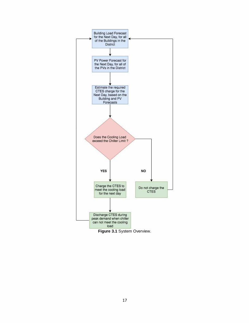
In this section, the framework of the proposed system is presented. In Figure 3.1

the system flow diagram is shown. The system starts by forecasting the building load

forecasts for the next day, these building are of different load profiles as shown earlier in

Figure 1.1. At the same time, the PV power forecasts are estimated for the next day as

well. Now based on these obtained forecasts for both the different buildings and for the

PV panel system, an estimate for the CTES charge is calculated, such that, all the

buildings cooling demand is met for the next day, during the peak demand period. In the

design of the chiller that serves all the buildings (shown in Figure 1.1), the peak capacity

of the chiller is less than the peak cooling demands, and the goal is to save in the capital

costs when initially installing the chiller, since the maximum chiller capacity is only used

in peak hours during only summer months, so, installing CTES will be more economically

visible, taking into consideration that the energy prices during peak hours is more than

the energy prices during off-peak hours. Now, if the buildings cooling load for the next

day does not exceed the chiller capacity, then the CTES is not charged.

17

Figure 3.1 System Overview.

18

3.2 Forecasting techniques

3.2.1 Multilayer Perceptron

The basic component of any MLP network is a neuron. A single neuron output is

calculated based on the summation of the incoming neurons values, originating from the

previous layers, then multiplied by the weights on these connections and added to a bias

term, finally applied to an activation function, as shown in Eq. (1). The structure of a single

neuron is shown Figure 3.2.

Figure 3.2 Neuron Structure

1

( )n

i i

i

f b w a=

= + , (1)

where b is the bias term; 𝑤𝑖 is the weight on each connection; 𝑎𝑖 is the value of each

incoming connection; 𝑛 is the total number of incoming connections for the neuron; f is

the activation function; and is the output value. The choice of the activation function

depends on the problem on hand. For time series predictions, Rectified Linear Unit

(ReLU) has proved to have the best accuracy performance compared to all other

activation functions. Eq. (2) shows the updated neuron output after applying the ReLU

activation function.

1

max(0, )n

i i

i

b w a=

= + . (2)

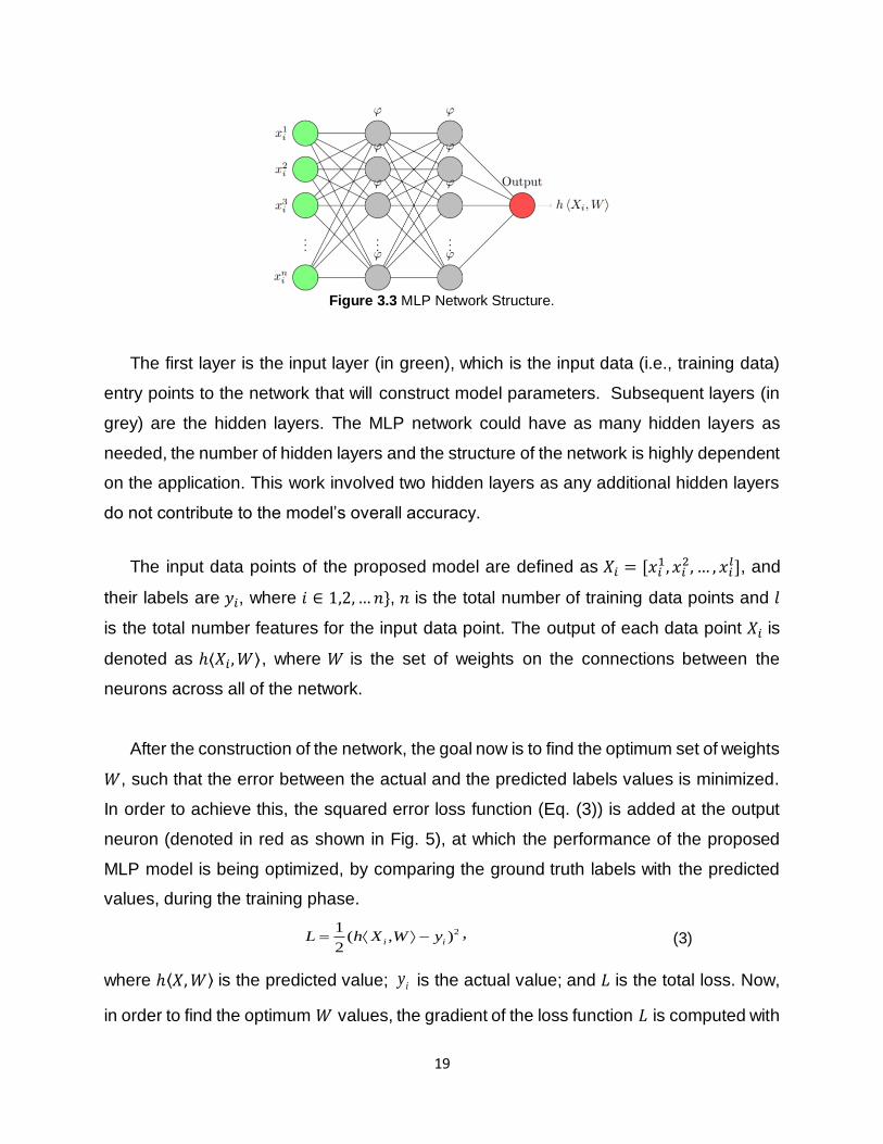
Neurons are only the building blocks of the MLP model. The basic structure of the

proposed model is illustrated in Figure 3.3.

19

Figure 3.3 MLP Network Structure.

The first layer is the input layer (in green), which is the input data (i.e., training data)

entry points to the network that will construct model parameters. Subsequent layers (in

grey) are the hidden layers. The MLP network could have as many hidden layers as

needed, the number of hidden layers and the structure of the network is highly dependent

on the application. This work involved two hidden layers as any additional hidden layers

do not contribute to the model’s overall accuracy.

The input data points of the proposed model are defined as 𝑋𝑖 = [𝑥𝑖1, 𝑥𝑖

2, … , 𝑥𝑖𝑙], and

their labels are 𝑦𝑖, where 𝑖 ∈ 1,2, … 𝑛}, 𝑛 is the total number of training data points and 𝑙

is the total number features for the input data point. The output of each data point 𝑋𝑖 is

denoted as ℎ⟨𝑋𝑖 , 𝑊⟩, where 𝑊 is the set of weights on the connections between the

neurons across all of the network.

After the construction of the network, the goal now is to find the optimum set of weights

𝑊, such that the error between the actual and the predicted labels values is minimized.

In order to achieve this, the squared error loss function (Eq. (3)) is added at the output

neuron (denoted in red as shown in Fig. 5), at which the performance of the proposed

MLP model is being optimized, by comparing the ground truth labels with the predicted

values, during the training phase.

2,1

( )2

i iL yh X W= − , (3)

where ℎ⟨𝑋, 𝑊⟩ is the predicted value; iy is the actual value; and 𝐿 is the total loss. Now,

in order to find the optimum 𝑊 values, the gradient of the loss function 𝐿 is computed with

20

respect to each weight on the network 𝑤𝑗→𝑘, where, 𝑗 and 𝑘 denote the neuron index; and

𝑤𝑗→𝑘 denotes the connection between neuron 𝑗 to neuron 𝑘. So, the gradient can be

expressed as shown in Eq. (4):

21( ) ( ) ,

2

( )

,

, , .

i

i

i

i

i k i k

i

i i k

i

L w yw

h X W

h h XyX W

w

wW

→ →

→

= −

= −

(4)

Finally, the gradient for each weight in the network is to be determined, until the

optimum value for each weight is reached, i.e., the overall loss is minimized. This would

be computationally expensive if classical optimization techniques, e.g., gradient decent,

are used. Thus, the Adam solver [51] was selected for solving this problem, which proved

to perform well on large datasets.

The structure of the implemented MLP network has seven neurons at the first hidden

layer and five neurons at the second hidden layer. The number of these neurons at these

different layers was selected by adding more neurons and keep tracking the Root Mean

Square Error (RMSE) performance, until the error is minimized over the training data.

Adding more neurons to the first or second hidden layers does not improve the model’s

overall accuracy.

3.2.2 Support Vector Regression

Support Vector Regression (SVR) is a supervised machine learning algorithm. It is

extension of Support Vector Machines (SVM) to regression problems. It solves the

following optimization problem:

*

*

, , ,1

*

*

1min ( ),

2

. .

( ) ,

( ) ,

, 0, 1,..., ,

nt

i iq

i

t

i i i

t

i i i

i i

q q C

s t

y q X

q X y

i n

=

+ +

− − +

− + +

=

(5)

21

where 𝑞 is the weight vector; 𝛽 is the bias term; ξ𝑖 , ξ𝑖∗ are the slack variables; C is a

tradeoff variable for the flatness of the curve; and ε is the tolerance variable; ( )iX is the

higher dimensional training vector resulted from iX . After solving the problem for 𝑞 and

𝛽, the test point label ˆiy can be predicted as follows:

ˆ , ( ) ,i iy q X = + (6)

where ⟨. , . ⟩ is the dot product of 𝑞 and ( )iX . Now, solving for the dual problem of Eq. (5)

and the introduction of the Lagrange multipliers, the final solution will be as follows:

*

1

ˆ ( ) ( , ) ,n

j i i i j

i

y K X X =

= − + (7)

where*,i i are the Lagrange multipliers and ( , )i jK X X is the kernel function used to find

the dot product between two without transforming them into the higher dimensional

space. Thus, the computational complexity would be lowered significantly, this is

commonly known as the kernel trick. SVR error performance could be improved by the

use of kernels as well. There are four known kernels used in the literature, linear, Radial

Basis Function (RBF), polynomial and sigmoid kernels. The RBF kernel has proved to

work well on regression problems in the literature, due to its computational efficiency [52].

In this work, RBF was used as kernel, the mathematical formulation for the kernel is as

follows:

2

22( , ) .

i jX X

i jK X X e

− −

= (8)

For SVR, similar steps were followed as the MLP. The C value that minimizes the

RMSE over the training data was chosen, the optimum C value in this work was found to

be 1000.

3.2.3 kNN Regression

kNN is a widely used clustering algorithm. However, it could also be implemented

to solve regression problems. For each test point 𝑥 the distance to all training datapoint

𝑥𝑖 is to be determined in the dataset as follows:

22

2ˆ( ) .j j

i i

j

D x x= − (9)

For each test point 𝑥 the distance to all training points 𝑥𝑖 is computed, then the k

nearest neighbors labels values 𝑦𝑖 are averaged to predict the 𝑥 label value �̂�. In this

work, kNN was optimized by changing the number of neighbors and tracking the RMSE

values over the training data. The RMSE value was at its minimum when the number of

neighbors 𝑘 is five. So, for all of the kNN models, the number of neighbors was chosen

to be 5.

3.2.4 Decision Tree Regression

Decision trees is a widely used machine learning algorithm, it can be used for both

classification and regression. It is constructed by nodes and leafs, each node has different

number of branches which would lead to another nodes or leafs. Each test point will start

from the root node, then will follow the branches that are tested to be true for that test

point, this procedure will be followed until a leaf is reached, then the predicted value ˆiy

of a test point is assigned a value as the value of the leaf that is has reached. The

construction of the tree could be done using different algorithms, one of most widely used

algorithm is Iterative Dichotomiser 3 (ID3), however, in this work we have implemented

the classification and regression trees (CART) algorithm, since it would also solve the

regression problem, and not restricted to the classification problem.

3.3 Models Input Variables

In order to see the best forecasting model for each variable (i.e. PV panel system,

mosque, clinic and office building), the model has been tested under different feature

selection schemes. At the beginning, the models were tested with only a single feature to

see the sensitivity of the model to this feature and how important is it. After the single

feature selection, different combinations of these features are fed to the forecasting

models.

23

Table 3-1 shows all the features used to forecast the four variables, namely, the

PV panel output power, the mosque demand, the clinic demand and the office building

demand.

Table 3-1 Input variables to the forecasting models.

Variable name Feature

𝑥𝑖1 Clear sky GHI

𝑥𝑖2 Clear sky DNI

𝑥𝑖3 Forecasted GHI

𝑥𝑖4 Forecasted DNI

𝑥𝑖5 Total cloud cover

𝑥𝑖6 Wind speed

𝑥𝑖7 Wind Direction

𝑥𝑖8 Temperature

𝑥𝑖9 Low cloud cover

𝑥𝑖10 Medium cloud cover

𝑥𝑖11 High cloud cover

𝑥𝑖12 Total Aerosol Optical Depth at 550nm

𝑥𝑖13 Dust Aerosol Optical Depth at 550nm

𝑥𝑖14 Hour

𝑥𝑖15 Month

𝑥𝑖16 Day of week

𝑥𝑖17 Day of year

𝑥𝑖18 PV generation at same hour and pervious day

𝑥𝑖19 mosque demand at same hour and previous week

𝑥𝑖20 clinic demand at same hour and previous week

𝑥𝑖21 office building demand at same hour and previous week

24

Each forecasting model (i.e. for PV panel system, mosque, clinic and office

building) has been tested under four different machine learning models and each one of

these machine learning models was tested under different feature selection schemes.

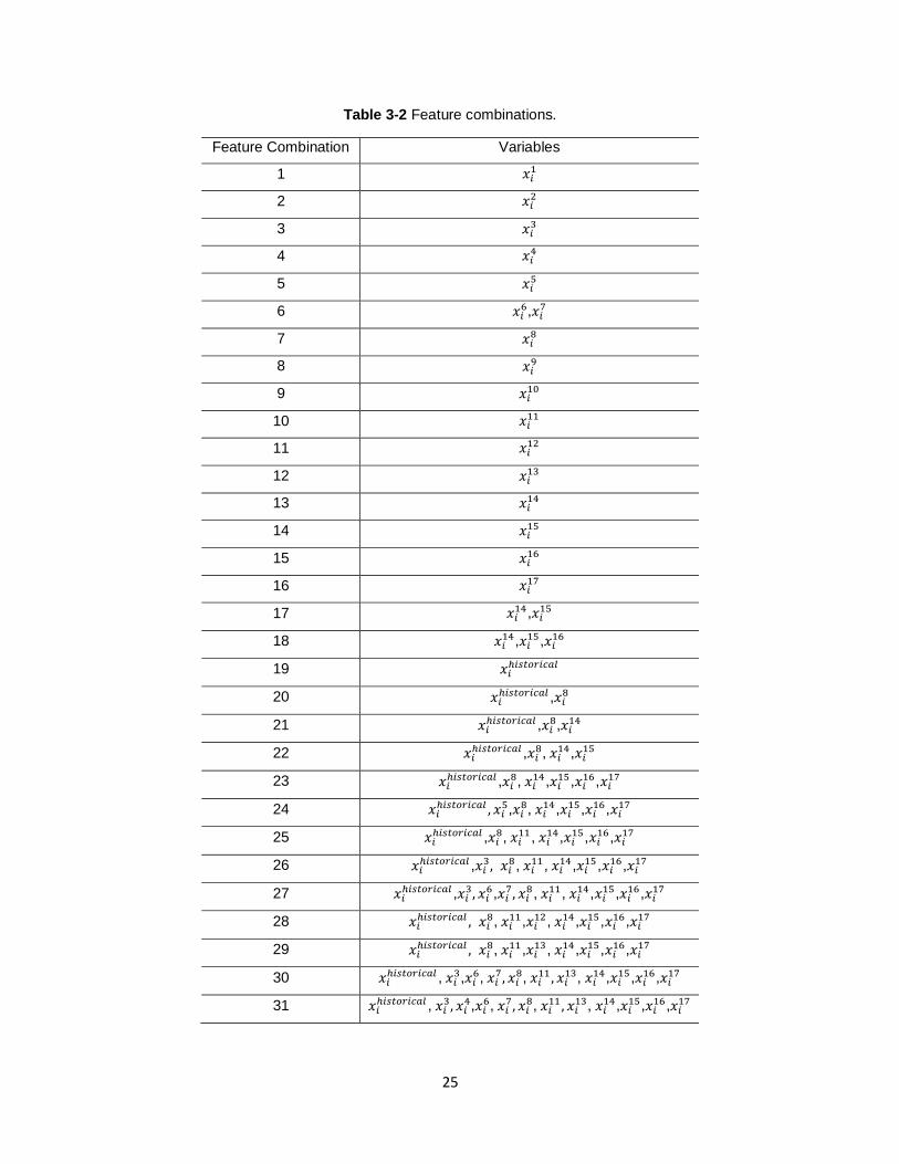
The different combinations of these feature selection schemes are listed in Table 3-2.

The variables 𝑥𝑖18 , 𝑥𝑖

19 , 𝑥𝑖20 and 𝑥𝑖

21 are defined as 𝑥𝑖ℎ𝑖𝑠𝑡𝑜𝑟𝑖𝑐𝑎𝑙 depending on each forecasted

variable. So, when we are doing forecasting for the PV panels generation 𝑥𝑖ℎ𝑖𝑠𝑡𝑜𝑟𝑖𝑐𝑎𝑙 refers

to 𝑥𝑖18 and when we are doing forecasting for the mosque the variable 𝑥𝑖

ℎ𝑖𝑠𝑡𝑜𝑟𝑖𝑐𝑎𝑙 refers to

𝑥𝑖19. Similar thing applies also to the remaining two variables (i.e. clinic and office building).

This definition is followed for simplicity. The variable 𝑥𝑖16 which refers to the day of the

week is only important when doing the forecasting for the different types of buildings, as

the behavior of these buildings is affected by the weekend/weekday behavior. However,

this is not true for the PV panel system forecasting, as the generation of the PV panels is

totally independent of the weekday/weekend schedule. Because of that, the variable 𝑥𝑖16

is not included in the PV panel forecasting model, and the variable 𝑥𝑖16 in Table 3-1 is

only applicable to the three buildings types (i.e. clinic, mosque and office building). And it

is not included in all of the forecasting models for the PV generation.

25

Table 3-2 Feature combinations.

Feature Combination Variables

1 𝑥𝑖1

2 𝑥𝑖2

3 𝑥𝑖3

4 𝑥𝑖4

5 𝑥𝑖5

6 𝑥𝑖6,𝑥𝑖

7

7 𝑥𝑖8

8 𝑥𝑖9

9 𝑥𝑖10

10 𝑥𝑖11

11 𝑥𝑖12

12 𝑥𝑖13

13 𝑥𝑖14

14 𝑥𝑖15

15 𝑥𝑖16

16 𝑥𝑖17


15


15,𝑥𝑖16

19 𝑥𝑖ℎ𝑖𝑠𝑡𝑜𝑟𝑖𝑐𝑎𝑙

20 𝑥𝑖ℎ𝑖𝑠𝑡𝑜𝑟𝑖𝑐𝑎𝑙 ,𝑥𝑖

8


8,𝑥𝑖14


8, 𝑥𝑖14,𝑥𝑖

15



15,𝑥𝑖16,𝑥𝑖

17

24 𝑥𝑖ℎ𝑖𝑠𝑡𝑜𝑟𝑖𝑐𝑎𝑙 , 𝑥𝑖

5,𝑥𝑖8, 𝑥𝑖


16,𝑥𝑖17


8, 𝑥𝑖11, 𝑥𝑖


16,𝑥𝑖17


3, 𝑥𝑖8, 𝑥𝑖

11, 𝑥𝑖14,𝑥𝑖


17




11, 𝑥𝑖14,𝑥𝑖


17



12, 𝑥𝑖14,𝑥𝑖


17



13, 𝑥𝑖14,𝑥𝑖


17


3,𝑥𝑖6, 𝑥𝑖


11 , 𝑥𝑖13, 𝑥𝑖


16,𝑥𝑖17




8, 𝑥𝑖11 , 𝑥𝑖

13, 𝑥𝑖14,𝑥𝑖


17

26

3.4 Model Evaluation and Error Measure

3.4.1 Error Measure

All of the forecasting models under the different feature selection schemes and

under different machine learning methods were tested also under multiple error metrics,

to better asses their performance. Each error metric has its own advantages and

drawbacks. In this section these error metrics are defined with an explanation for each

method.

Root Mean Squared Error (RMSE) is the first error metric used, it is widely used in

the literature and is defined as follows:

𝑅𝑀𝑆𝐸 = √∑ (�̂�𝑖 − 𝑦𝑖)2𝑛

𝑖=1

𝑛, (10)

�̂�𝑖 is the forecasted value at the time 𝑖; 𝑦𝑖 is the ground truth or actual reading at time 𝑖

and 𝑛 represents the total number of test points in the test dataset. The main advantage

of RMSE is that the results of the error are in the same unit as the forecasted value, in

this work the unit for the PV panel system and the buildings is 𝑊𝑎𝑡𝑡𝑠, which is the

instantons power generation or consumption. RMSE is sensitive to the outliers compared

to the other error metrics.

The second error metric used in this work is the normalized RMSE (nRMSE), it is

basically calculated similar as the RMSE but the final result is divided by the maximum

value in the test dataset, it is defined as follows:

𝑛𝑅𝑀𝑆𝐸(%) =√∑ (�̂�𝑖 − 𝑦𝑖)2𝑛

𝑖=1𝑛

𝑦𝑚𝑎𝑥× 100,

(11)

where 𝑦𝑚𝑎𝑥 is the maximum value in the test dataset. The nRMSE is a percentage error,

hence, it has no unit. Normalized error such as the nRMSE are a good option when

comparing the error across different dataset, as each dataset would have a different

maximum value, hence, a normalization approach is required to compare the

performance of these different datasets.

Third error metric used in this work is the Mean Absolute Percentage Error

(MAPE), it is defined as follows:

27

𝑀𝐴𝑃𝐸(%) =100

𝑛∑ |

�̂�𝑖 − 𝑦𝑖

𝑦𝑖|

𝑛

𝑖=1

. (12)

MAPE is also a percentage error and it is a good option when comparing the

performance of different dataset. It has the issue of dividing by zero and also it could

reach values more that 100% depending on the forecasting accuracy.

Fourth error metric used is the Mean Absolute Error (MAE), is can be found using

the average absolute different between the predicted and the actual values across the

testing dataset, is it given as follows:

𝑀𝐴𝐸 =1

𝑛∑|�̂�𝑖 − 𝑦𝑖|

𝑛

𝑖=1

, (13)

MAE has the same units as the tested variable and is less sensitive to outliers when

compared to RMSE, that’s mainly because of the absence of the square term in the

equation.

Last error metric used is the normalized MAE (nMAE). It is also calculated in a

similar manner as the MAE, but by dividing over the maximum test value in the test

dataset, the nMAE is defined as follows:

𝑛𝑀𝐴𝐸(%) =1

𝑛∑

|�̂�𝑖 − 𝑦𝑖|

𝑦𝑚𝑎𝑥

𝑛

𝑖=1

× 100, (14)

The five error metrics defined earlier were all used to assess the performance of the

forecasting models.

3.4.2 Smart Persistence

Smart persistence is the benchmark model implemented in this work only in the

initial case study, when doing the irradiation forecasting, it is based on the deterministic

irradiance variation from time 𝑡 and time 𝑡 + 𝑇, calculated from the clear sky model. The

smart persistence mathematical formulation is as follows:

28

𝐼𝑠𝑝(𝑡 + 𝑇) =𝐼𝑐𝑠(𝑡 + 𝑇)

𝐼𝑐𝑠(𝑡)𝐼(𝑡), (15)

where 𝐼𝑠𝑝(𝑡 + 𝑇) is the smart persistence irradiance prediction at time 𝑡 + 𝑇, 𝐼𝑐𝑠(𝑡 + 𝑇) is

the clear sky model at time 𝑡 + 𝑇 , 𝐼𝑐𝑠(𝑡) is the clear sky model at time 𝑡 , 𝐼(𝑡) is the

irradiance observed value at time 𝑡. The Ineichen and Perez clear sky model [53, 54] was

used in this work.

3.4.3 Forecast Skill

The performance of the forecasting models need to be normalized by a

benchmark. The forecast skill proposed in [55], is a way to normalize and compare the

accuracy of the model against the benchmark model. The mathematical formulation of

the forecast skill is as follows:

𝐹𝑆 = 1 −𝑅𝑀𝑆𝐸𝑚𝑜𝑑𝑒𝑙

𝑅𝑀𝑆𝐸𝑠𝑝, (16)

where 𝐹𝑆 is the forecast skill value, 𝑅𝑀𝑆𝐸𝑚𝑜𝑑𝑒𝑙 is the RMSE value resulted from the

forecasting model, 𝑅𝑀𝑆𝐸𝑠𝑝 is the RMSE resulted from the smart persistence model. A

forecast skill of 0 indicates that the model performance is similar to the smart persistence

model. A higher positive 𝐹𝑆 value indicates that the model has a better performance

compared to the smart persistence model, with a maximum 𝐹𝑆 value of 1. A negative 𝐹𝑆

value indicates that the forecasting model performs worse than the smart persistence

model.

3.5 Control Strategy for the CTES

The control strategies for the CTES has been already discussed in the literature

review section. Basically, there are two main types of the CTES in terms of the cooling

capacity. The first one is the full storage system, where the cooling demand is met totally

by the CTES during the peak hours. The second type is the partial CTES, where the

cooling load is met partially by the CTES during the peak hours, while the remaining

cooling demand is met by the existing chiller capacity. In this work, the partial storage

system is proposed.

29

Chapter 4 Data

The data in this work were collected from four different resources, the following sub-

sections discuss in detail the data resources, their resolution and cleaning methods.

4.1 PV panel data

The PV panel data were collected starting from 03-Jun-2016 until 31-08-2018. The

PV panel system is placed on a rooftop of a mosque in Riyadh, Saudi Arabia. The PV site

has a peak capacity of 120 kW and it has a total of 5 inverters. The inverters were installed

over time, and all of them were fully operational by 15-Jul-2016. The site has a power

reading every 1-minute and it is managed by King Abdulaziz City for Science and

Technology (KACST) and Saudi Electricity Company (SEC) in a joint project. The data

were provided as a 1-hour resolution data, using backward average. For example, the

data collected from 10:01 a.m. to 11:00 a.m. are averaged across the period and then

given as the value for 11:00 a.m. We then subtracted 1-hour from these readings, such

that the 11:00 a.m. reading is 10:00 a.m., that’s basically to make the data forward

averaged as in the remaining datasets. The maximum reading in the dataset is 105,928.5

Watts on 25-Mar-2018 at 11:00 a.m. This is mainly because the sun is almost

perpendicular to the solar PV panels during the month of March for the tested location.

The tilt angle is kept fixed at 24 during the whole year. Any reading in the dataset with

value less than 100 Watts is considered zero. The data have a few missing dates, where

the readings are None, and these days were omitted from the dataset. The seasonality

of the PV panel system is on a daily basis, meaning that, the pattern of the PV power

curve repeats itself on a daily basis. Because of that, we have added the PV power

generation for the past day as a feature to forecast the PV output for the next day.

30

4.2 Buildings Load Data

The building data were provided by SEC, which has three building types: mosque,

health clinic and an office building. The demand reading for the buildings has a reading

every 30 minutes, the reading is for the instantaneous power, given in the form HH:MM,

where the HH represents the local time in hours and MM represents the local time in

minutes. All the data for the three buildings have two readings each hour, one at HH:00

and the other at HH:30. In order to do the forward average reading for each hour, the data

were interpolated to minutely resolution, such that the readings for each hour has 60

readings, then the average for each hour is found by averaging these 60 readings over

the hour, using forward average. Performing the interpolation then taking the average

again lead to a better average than just taking the two values recorded at HH:00 and.

HH:30, because the latter way ignores the load in the next half-hour and will not

considered in the average, while the interpolation then averaging approach takes into

account the power reading in the next half-hour. Each load profile in the proposed work

is different from the others in terms of the load profile characteristics. The details of each

load profile are discussed in the following subsections.

4.2.1 Mosque

The daily load profile of the mosque is shown in Figure 4.1. The mosque load

varies greatly over the day and night. The mosque load profile has multiple spikes over

the day, which occur during the prayer times (5 prayers a day). Each prayer has a known

time, which is correlated with solar time, hence, can be converted to local time. As seen

from Figure 4.1 the maximum load occurs during the midday, when the temperatures is

at it’s peak causing the cooling demand to reach its peak as well. The lowest demands

are during the first prayer, which is before sunrise, and at the end of the night, when the

mosque is at its coolest point, causing the cooling demand to drop to its lowest. This is

seen from Figure 4.1. The peak demand of the mosque occurs during the second and

the third prayer, that is around the midday for the second prayer, hence the cooling

demand is high during that time. The seasonality of the mosque load profile is weekly,

that’s because the Friday prayer occurs once a week during the midday, and this prayer

31

is crowded more than the other prayers during the other days of the week. Moreover, the

mosque is more crowded during the weekends, as for the second and third prayer during

the workdays, people are at their work, and they pray at their work place. Because of that,

we chose the seasonality of the mosque to be weekly, and we fed the forecasting model

for the mosque the demand for the previous week at the same day and hour. The

maximum reading for the power meter during the whole period for the mosque is 160,80

kW. While the minimum is 700 W and the standard deviation is 29,65 kW.

Figure 4.1 Mosque load profile for 21-Jul-2017.

4.2.2 Clinic

The clinic load profile is shown in Figure 4.2, the load has much less variability when

compared with the mosque. The load is smooth and peaks around 4:00 p.m. (local time).

The minimum load is around 40 kW, while the maximum is around 50 kW, that’s 25%

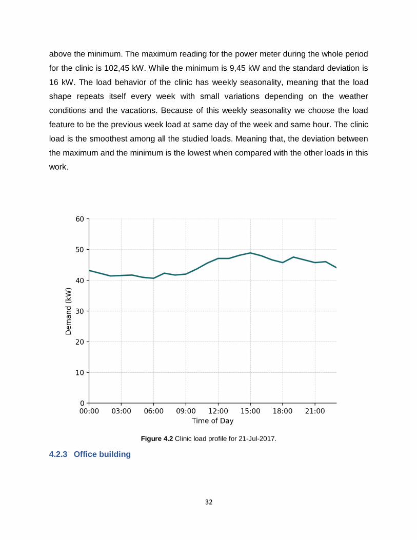
32

above the minimum. The maximum reading for the power meter during the whole period

for the clinic is 102,45 kW. While the minimum is 9,45 kW and the standard deviation is

16 kW. The load behavior of the clinic has weekly seasonality, meaning that the load

shape repeats itself every week with small variations depending on the weather

conditions and the vacations. Because of this weekly seasonality we choose the load

feature to be the previous week load at same day of the week and same hour. The clinic

load is the smoothest among all the studied loads. Meaning that, the deviation between

the maximum and the minimum is the lowest when compared with the other loads in this

work.

Figure 4.2 Clinic load profile for 21-Jul-2017.

4.2.3 Office building

33

The office building load profile is shown in Figure 4.3, the peak demand occurs

around 1 p.m. (local time). While the minimum occurs at around 7-8 a.m., that’s just before

the employees come to work. The maximum demand is around 100 kW, while the

minimum is around 75 kW. The maximum reading for the power meter during the whole

period for the office building is 147,68 kW. While the minimum is 30,4 kW and the

standard deviation is 18,8 kW. As the previous two loads, the load behavior of the office

building has weekly seasonality. Because of this weekly seasonality we choose the load

feature to be the previous week load at same day of the week and same hour. The office

building load is in the middle when it comes to the variations in the load when compared

with the other two loads, the mosque and the clinic.

Figure 4.3 Office building load profile for 21-Jul-2017.

34

4.3 CAMS near-real time global atmospheric composition

service data

The CAMS near-real time global atmospheric composition service data is a

satellite dataset that has been processed to estimate the atmospheric composition at a

global scale. The CAMS data is available every 3-hours and it is averaged forward. In

order to have a 1-hour resolution data, we performed a linear interpolation for the hours

in between, such that we have an atmospheric reading every hour. The CAMS data have

lots of features to choose from, the list of available features can be found here1. The data

have AOD readings at multiple wavelengths (i.e., 469, 550, 670, 865 and 1240 nm). The

data have also the estimates for the particulate matter pm at different scales from 1 to 10

µm, temperature estimated at two meters above the ground and wind direction at 2 meters

above the ground. Multiple grid sizes are available through CAMS, in this work we have

used the smallest available grid size, which is 0.125° × 0.125° that contains the site under

test. The service is implemented by European Center for Medium-Range Weather

Forecasts (ECMWF).

4.4 CAMS radiation service

The CAMS radiation service is a service that provides the radiation forecasts for

the GHI, DNI and DHI on horizontal surface. The forecasts are estimated for both the

clear sky conditions and for the actual weather conditions taken from the CAMS near-

real-time. The provided forecasts are available on a monthly, daily, hourly and up-to 1-

minute resolution. The hourly data is used in this work. The data can be downloaded from

here2. The data from this dataset is forward averaged as the remaining datasets in this

work.

4.5 Data Splitting

1 https://apps.ecmwf.int/datasets/data/cams-nrealtime/ 2 http://www.soda-pro.com/web-services/radiation/cams-radiation-service

35

After all the data has been cleaned and as described in earlier sections, all the

data from the four different resources has been integrated together using the timestamp

information. The total number of features of this integrated dataset is shown in Table 3-1,

which includes all the tested features. Now, after integrating the datasets and before

training the forecasting models, the data has been split into training and testing. The

training dataset is used to train the forecasting models (i.e. Decision Trees, kNN, etc.).

While the testing data is used to test the model performance after the model has been

trained. We split the data into 80% as training data and the rest 20% is used as testing

data. The data splitting is random across the dataset, this way we can insure that the test

data has contains different days, hours and weather conditions. The training data and test

data are the same across all the models. Meaning that, the training data used to train the

kNN and the remaining forecasting methods are the same. Similar this also applies to the

testing data.

4.6 Data Normalization

Each of the features shown in Table 3-1 in the dataset has different maximum and

minimum values. So, features with higher values would impact the model more when

performing the forecasting. In order to make all the features have the similar impact

initially on the forecasting model, a data normalization technique has been used before

training the data. The data normalization used in the work is shown in Eq. (17):

𝑥𝑛𝑜𝑟𝑚 =𝑥𝑖 − �̅�𝑖

𝜎, (17)

where 𝑥𝑛𝑜𝑟𝑚 is the normalized feature, 𝑥𝑖 is the original feature value, �̅�𝑖 is the mean value

across that feature and 𝜎 is the standard deviation for that specific feature.

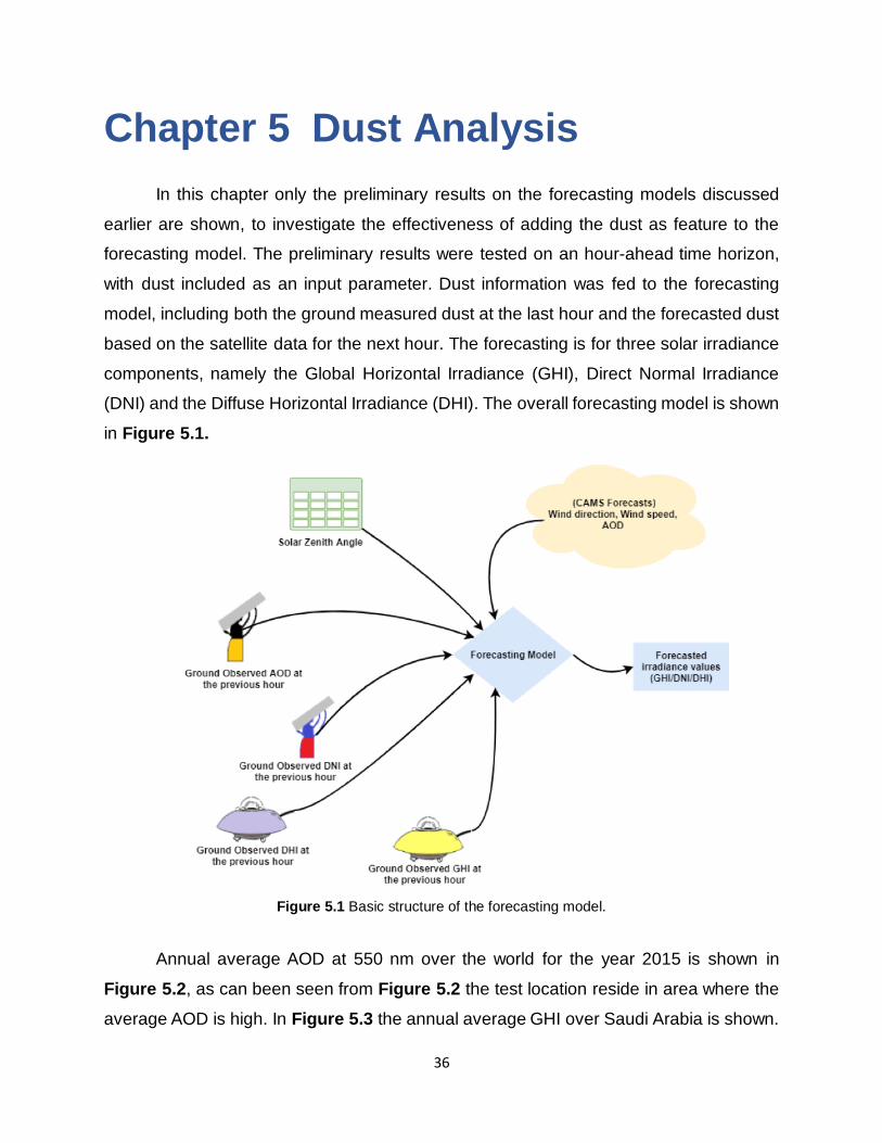
36

Chapter 5 Dust Analysis

In this chapter only the preliminary results on the forecasting models discussed

earlier are shown, to investigate the effectiveness of adding the dust as feature to the

forecasting model. The preliminary results were tested on an hour-ahead time horizon,

with dust included as an input parameter. Dust information was fed to the forecasting

model, including both the ground measured dust at the last hour and the forecasted dust

based on the satellite data for the next hour. The forecasting is for three solar irradiance

components, namely the Global Horizontal Irradiance (GHI), Direct Normal Irradiance

(DNI) and the Diffuse Horizontal Irradiance (DHI). The overall forecasting model is shown

in Figure 5.1.

Figure 5.1 Basic structure of the forecasting model.

Annual average AOD at 550 nm over the world for the year 2015 is shown in

Figure 5.2, as can been seen from Figure 5.2 the test location reside in area where the

average AOD is high. In Figure 5.3 the annual average GHI over Saudi Arabia is shown.

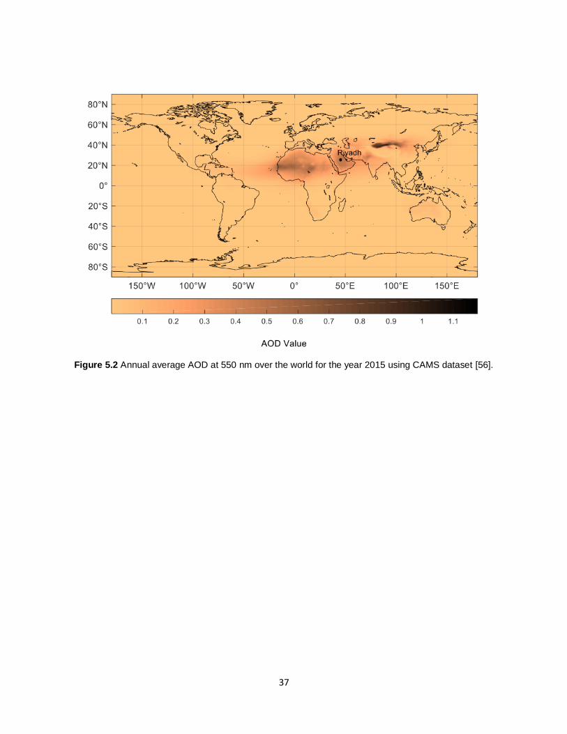
37

Figure 5.2 Annual average AOD at 550 nm over the world for the year 2015 using CAMS dataset [56].

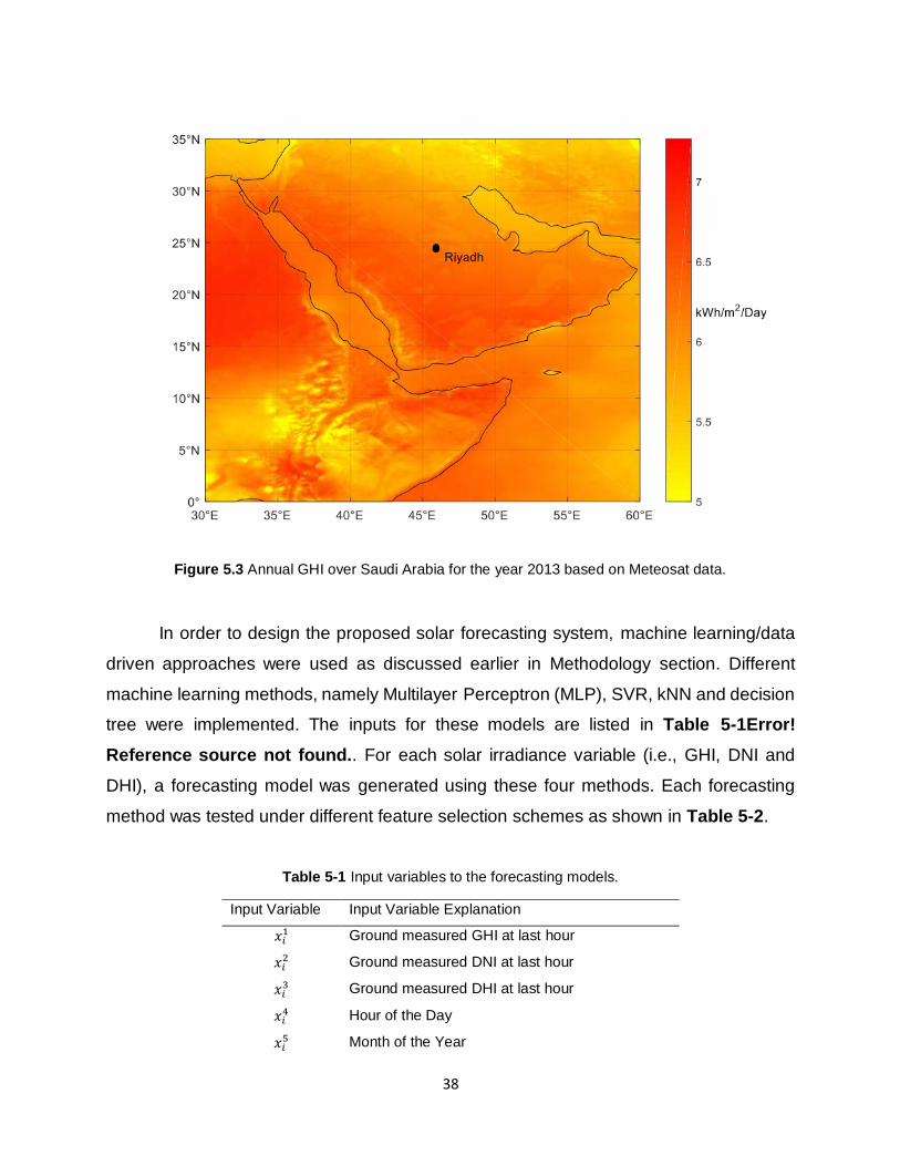
38

Figure 5.3 Annual GHI over Saudi Arabia for the year 2013 based on Meteosat data.

In order to design the proposed solar forecasting system, machine learning/data

driven approaches were used as discussed earlier in Methodology section. Different

machine learning methods, namely Multilayer Perceptron (MLP), SVR, kNN and decision

tree were implemented. The inputs for these models are listed in Table 5-1Error!

Reference source not found.. For each solar irradiance variable (i.e., GHI, DNI and

DHI), a forecasting model was generated using these four methods. Each forecasting

method was tested under different feature selection schemes as shown in Table 5-2.

Table 5-1 Input variables to the forecasting models.

Input Variable Input Variable Explanation

𝑥𝑖1 Ground measured GHI at last hour

𝑥𝑖2 Ground measured DNI at last hour

𝑥𝑖3 Ground measured DHI at last hour

𝑥𝑖4 Hour of the Day

𝑥𝑖5 Month of the Year

39

𝑥𝑖6 Solar Zenith Angle

𝑥𝑖7 Wind Speed

𝑥𝑖8 Wind Direction

𝑥𝑖9 CAMS AOD at 550 nm

𝑥𝑖10 AERONET AOD at 550 nm observed at last hour

𝑥𝑖11 Angstrom Exponent α

Table 5-2 GHI/DNI/DHI forecasting model feature selection schemes.

Variable Feature Selection Scheme Input Variables

GHI

1 𝑥𝑖1, 𝑥𝑖

4, … , 𝑥𝑖7

2 𝑥𝑖1 , 𝑥𝑖

4 , … , 𝑥𝑖9


4, … , 𝑥𝑖8, 𝑥𝑖

10, 𝑥𝑖11

DNI


4, … , 𝑥𝑖7


4, … , 𝑥𝑖9


4, … , 𝑥𝑖8, 𝑥𝑖

10, 𝑥𝑖11

DHI


4, … , 𝑥𝑖7


4, … , 𝑥𝑖9


4, … , 𝑥𝑖8, 𝑥𝑖

10, 𝑥𝑖11

In the next sections the datasets are discussed and analyzed, the final section

shows the results for this preliminary case study.

5.1 Datasets

The datasets used in this preliminary case study were collected from KACARE,

AERONET, and CAMS, covering the period of three years from January 14th, 2013 to

December 31st, 2015 with a temporal resolution of one-hour. The data collection, cleaning

and quality assurance techniques for each dataset are discussed below.

5.1.1 KACARE dataset

KACARE is a government agency responsible for the renewable energy legislation,

analysis, measurements and research in Saudi Arabia. In 2013, KACARE started

Renewable Recourse Monitoring and Mapping (RRMM) Solar Measurement Network.

40

The goal of this RRMM Solar Measurement Network is to provide accurate ground-based

measurements of solar radiation alongside the relevant weather parameters across the

country. The total number of stations in the network is 53 [57].

The KACARE dataset used in this work was collected in Riyadh, Saudi Arabia, with

exact site information as shown in the Table 5-3.

Table 5-3 KACARE site information.

Latitude 24.90693° North

Longitude 46.39729° East

Elevation 764.0 Meters

The used measurement instruments are shown in Table 5-4.

Table 5-4 List of measurement Instruments.

Parameter Equipment Units Uncertainty Details

Relative

Humidity Relative Humidity Probe % RH

+/- 3%

to +/- 7% Primary

GHI Pyranometer 2W/m +/- 2.0% Primary

GHI Rotating Shadowband Radiometer

2W/m +/- 5.0% Secondary

DNI Pyrheliometer 2W/m +/- 2.0% Primary

DNI Rotating Shadowband Radiometer


DHI Pyranometer 2W/m +/- 2.0% Primary

DHI Rotating Shadowband Radiometer


AOD CIMEL C-318

Sunphotometer No unit +/- 0.01 OD Primary

KACARE data are collected every minute during daytime, containing GHI, DNI,

DHI and relative humidity readings. In this work, we have computed the one-hour average

of these 1-min readings. So, for each hour HH:MM, we average all the minutes MM in

41

that hour from MM=00 to MM=59, then use this averaged (GHI/DNI/DHI) value in the

tested models as 𝑥𝑖1, 𝑥𝑖

2 and 𝑥𝑖3. In order to have more robust measurements, a secondary

Pyranometer similar in make and model was installed at the same site to measure GHI,

plus the rotating shadowband radiometer listed in Table 5-4. Data is collected from the

secondary equipment in case of the failure of the primary equipment. The last column in

the Table 5-4 shows whether the equipment was used as a primary or a secondary for

the measurements. For post processing data quality assurance NREL’s Solar Energy

Research Institute Quality Control (SERI-QC) procedures were followed [58]. Data can

be requested through KACARE Atlas website (KACARE; https://rratlas.kacare.gov.sa/)

5.1.2 AERONET dataset (AERONET; https://aeronet.gsfc.nasa.gov/)

The AERONET program is a remote sensing ground-based measurement network

supported by NASA and many international institutions around the world. Their goal is to

measure the AOD across different locations in the world and provide these

measurements, alongside with microphysical properties, as an open access data.

AOD is a measure of the attenuation of radiation due to aerosols. AOD has no unit of

measurements, i.e., unitless. The minimum AOD value is zero, which indicates that the

atmosphere is clear. AOD value of 1 or more indicates a severe dust storm present in the

scene. Depending on the type of aerosols to be estimated, AOD is measured at multiple

wavelengths. In this work, the focus is to investigate the effect of dust, which is measured

at 550 nm, using both ground-based and satellite-based measurements.

AOD equipment for the tested site is located at the same coordinates shown in Table

5-3. This site has AOD readings at seven different wavelengths (i.e., 340, 380, 440, 500,

670, 870 and 1020 nm), as well as water vapor, solar zenith angle and the angstrom

values. This study focuses on the wavelengths at 440 and 670, since they are used to

extrapolate the AOD value at 550 nm, at which the dust concentration in the air is being

measured. The extrapolation of AOD at 550 nm can be calculated as follows:

42

22 1

1

exp(ln( ) ln( )),

= − (18)

where 1 is the AOD at 440 nm; α is the Angstrom Exponent and it is a good indicator for

the aerosol particle size in the air, α ≤ 1 indicates that the AOD particle distribution is

mainly dominated by coarse mode particles, while α ≥ 2 represents an AOD distribution

that is mainly dominated by a fine mode particles [59], 2 is the desired AOD at 550 nm,

at which the dust accumulation in the air is being measured. 1 and 2 are the

wavelengths at 550 nm and 440 nm. Angstrom Exponent α can be found using the AOD

readings at 440 nm and 670 as follows:

3 1

3 1

ln( ) ln( ),

ln( ) ln( )

−=

− (19)

where 3 is the AOD value at 670 nm and 3 is the wavelength at 670 nm.

The dataset has multiple readings every hour without consistency in data reading

intervals. However, in most of the days there is at least one reading every hour. If multiple

readings are recorded for an hour HH:MM, all the readings through that hour (MM=00 to

MM=59) are averaged, hence, we have one value per hour, this value is denoted as 𝑥𝑖10

as shown in Table 5-1. If one hour has a no readings, then the missing reading at this

hour is substituted by implementing a linear interpolation. Figure 5.4 shows histogram of

how many distinct hours the AERONET AOD readings are measured each day for the

tested site.

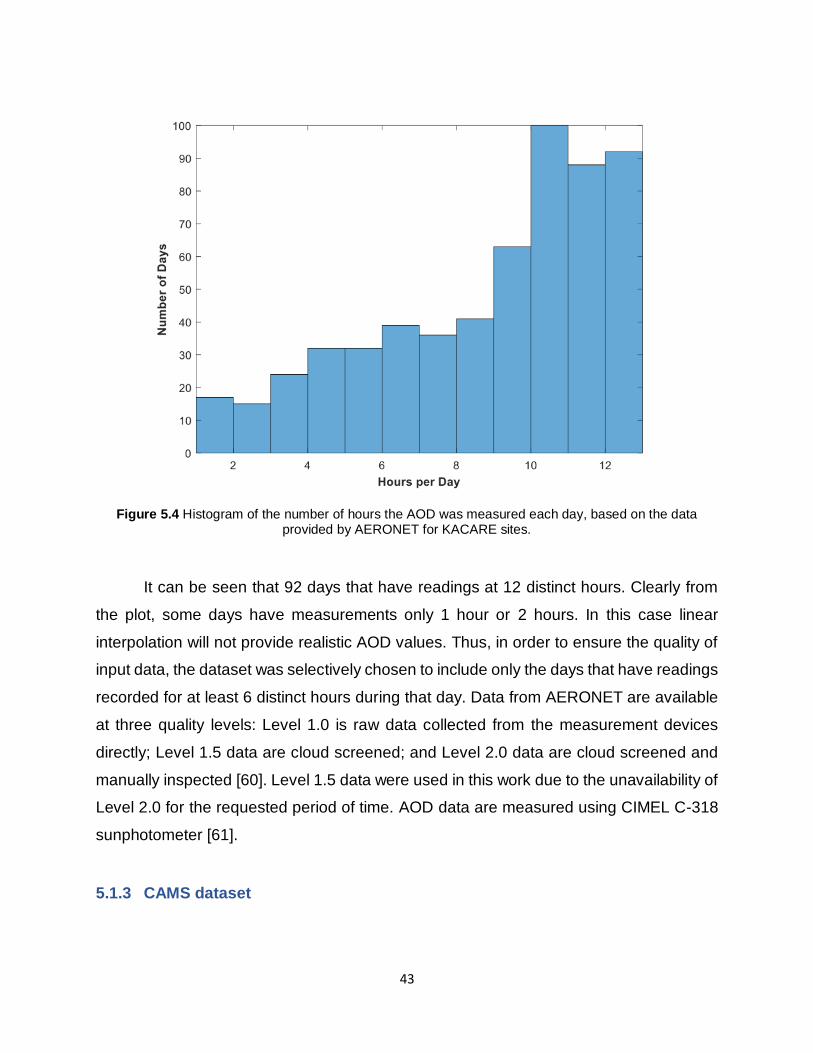
43

Figure 5.4 Histogram of the number of hours the AOD was measured each day, based on the data provided by AERONET for KACARE sites.

It can be seen that 92 days that have readings at 12 distinct hours. Clearly from

the plot, some days have measurements only 1 hour or 2 hours. In this case linear

interpolation will not provide realistic AOD values. Thus, in order to ensure the quality of

input data, the dataset was selectively chosen to include only the days that have readings

recorded for at least 6 distinct hours during that day. Data from AERONET are available

at three quality levels: Level 1.0 is raw data collected from the measurement devices

directly; Level 1.5 data are cloud screened; and Level 2.0 data are cloud screened and

manually inspected [60]. Level 1.5 data were used in this work due to the unavailability of

Level 2.0 for the requested period of time. AOD data are measured using CIMEL C-318

sunphotometer [61].

5.1.3 CAMS dataset

44

CAMS is one of the Copernicus programs aimed to provide data on atmospheric

composition at regional and global scale. It is managed by the European Commission

(EU), in partnership with European Space Agency (ESA), the European Organization for

the Exploitation of Meteorological Satellites (EUMETSAT) and the ECMWF.

The data contains many air quality parameters. It has AOD readings at five different

wavelengths (i.e., 469, 550, 670, 865 and 1240 nm), Particulate Matter at different

diameters (i.e., 10, 2.5, 1 µm), plus other weather parameters, such as temperature, wind

speed, dew point temperature, cloud cover and albedo.

The CAMS system utilizes AOD data retrieved from both Polar Multi-Sensor Aerosol

Product (PMAP) provided by EUMETSAT, alongside with the AOD data retrieved from

Moderate Resolution Imaging Spectroradiometer (MODIS) provided by NASA.

A grid size of 0.5° × 0.5° that contains the site indicated in Table 5-3 was used in

this work. The temporal resolution of the CAMS data is based on 3 hours forecasting step,

starting from 00:00 UTC to 21:00 UTC for each day, so, for each day the available

forecasts are for the hours 00:00, 03:00, 06:00, 09:00, 12:00, 15:00, 18:00 and 21:00, a

total of 8 readings. In order to match the temporal resolution of the CAMS readings with

other KACARE and AERONET datasets readings, a linear interpolation was performed

on CAMS dataset, such that, a one reading was made available at each hour of the day.

In this work, we implemented an hour-ahead forecasting model, hence, we used the

forecasted CAMS AOD value for the next hour, which was already interpolated as

discussed above. This CAMS AOD value is fed into the model as 𝑥𝑖9, as shown in Table

5-1Error! Reference source not found.. All of CAMS data used in this work are available

through ECMWF website (ECMWF; https://www.ecmwf.int/).

5.2 Data analysis

This section provides some insights and analysis about the dataset implemented in

this work. Figure 5.5 shows a windrose plot alongside with dust AOD values for the site

45

under study in Riyadh, Saudi Arabia. The location is surrounded by two deserts, the Rub’

Al-khali desert from the South and South East and Addahna desert from the North East.

This makes the selected site a perfect choice for this work.

Figure 5.5 Windrose plot versus AOD values.

As can be clearly seen from the plot, the AOD values are highly dependent on the

wind direction. The southern winds would have a higher chance of carrying dust particles,

and in the second place the northern winds with a lower chance. This could be

understood, knowing the fact that there is a large sand dessert laying at the southern side

of the site, and another large desert laying at the northeastern side. Thus, any wind

originating from these directions would have a higher probability of carrying sand

particles, hence increasing the AOD value. Conversely, winds coming from the western

side would have a lower probability of carrying dust particles. Therefore, dust intensity in

the air is highly dependent on the wind direction. Accordingly, the solar irradiance is

dependent on wind direction as well.

A scatter density plot to compare AERONET AOD at 550 nm (𝐴𝑂𝐷550) and CAMS

𝐴𝑂𝐷550 values is shown in Figure 5.6. As can be clearly seen, CAMS 𝐴𝑂𝐷550 seems to

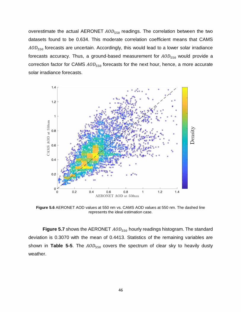
46

overestimate the actual AERONET 𝐴𝑂𝐷550 readings. The correlation between the two

datasets found to be 0.634. This moderate correlation coefficient means that CAMS

𝐴𝑂𝐷550 forecasts are uncertain. Accordingly, this would lead to a lower solar irradiance

forecasts accuracy. Thus, a ground-based measurement for 𝐴𝑂𝐷550 would provide a

correction factor for CAMS 𝐴𝑂𝐷550 forecasts for the next hour, hence, a more accurate

solar irradiance forecasts.

Figure 5.6 AERONET AOD values at 550 nm vs. CAMS AOD values at 550 nm. The dashed line represents the ideal estimation case.

Figure 5.7 shows the AERONET 𝐴𝑂𝐷550 hourly readings histogram. The standard

deviation is 0.3070 with the mean of 0.4413. Statistics of the remaining variables are

shown in Table 5-5. The 𝐴𝑂𝐷550 covers the spectrum of clear sky to heavily dusty

weather.

47

Figure 5.7 AERONET AOD at 550 nm histogram.

Table 5-5 Variables mean and standard deviation.

Mean Standard

Deviation Unit

GHI 620.34 272.96 W/m2

DNI 567.11 242.26 W/m2

DHI 221.63 112.82 W/m2

Wind Speed 4.212 1.75 m/s

AERONET 𝐴𝑂𝐷550 0.4413 0.3070 --

CAMS 𝐴𝑂𝐷550 0.5375 0.2569 --

Figure 5.8 shows the average monthly 𝐴𝑂𝐷550 for the test site, starting from 2013

to 2015, for both the AERONET and CAMS datasets. April then May have the highest

𝐴𝑂𝐷550 among all the other months in both datasets. Moreover, CAMS dataset appears

to overestimate the 𝐴𝑂𝐷550 values most of the year except for the months starting from

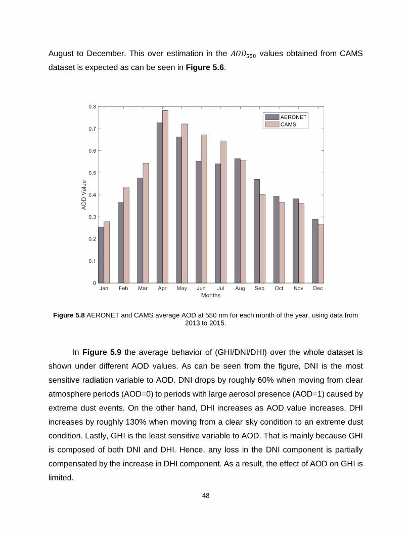
48

August to December. This over estimation in the 𝐴𝑂𝐷550 values obtained from CAMS

dataset is expected as can be seen in Figure 5.6.

Figure 5.8 AERONET and CAMS average AOD at 550 nm for each month of the year, using data from 2013 to 2015.

In Figure 5.9 the average behavior of (GHI/DNI/DHI) over the whole dataset is

shown under different AOD values. As can be seen from the figure, DNI is the most

sensitive radiation variable to AOD. DNI drops by roughly 60% when moving from clear

atmosphere periods (AOD=0) to periods with large aerosol presence (AOD=1) caused by

extreme dust events. On the other hand, DHI increases as AOD value increases. DHI

increases by roughly 130% when moving from a clear sky condition to an extreme dust

condition. Lastly, GHI is the least sensitive variable to AOD. That is mainly because GHI

is composed of both DNI and DHI. Hence, any loss in the DNI component is partially

compensated by the increase in DHI component. As a result, the effect of AOD on GHI is

limited.

49

Figure 5.9 (GHI/DNI/DHI) biases under different AOD values.

5.3 Results and discussion

The forecasting model basic structure is shown in Figure 5.1. The input variables for

GHI/DNI/DHI forecasting models are listed in Table 5-1Error! Reference source not

found. & Table 5-2. The construction of each forecasting method and the different

subsets of the selected parameters are discussed earlier.

Table 5-6 shows the GHI results using the testing data under these different methods

and feature selection schemes. Each row in Table 5-6 represents a set of selected

features and each column represents the forecasting method used. For the first row in

Table 5-6, features 𝑥𝑖1, 𝑥𝑖

4, … , 𝑥𝑖8 are considered, they represent a set of features as

described in Table 1, these features are considered the basic feature selection scheme

in this work. As we move to the next row, when the CAMS 𝐴𝑂𝐷550 𝑥𝑖9 is added to the

model, an improvement can be seen in all the models except for the kNN. Now, as we

50

move to the last row, when we remove the CAMS 𝐴𝑂𝐷550 𝑥𝑖9 and add both the AERONET

𝐴𝑂𝐷550 𝑥𝑖10 and the angstrom exponent 𝑥𝑖

11 , improvement was observed in all tested

models. When comparing the FSs for the MLP, kNN and SVR in the last row with the

CAMS 𝐴𝑂𝐷550 model, an improvement of around 9%, 2% and 0.45% was observed,

respectively. As can be seen from Table 6, when the new features are added, the RMSE

and FS results for the MLP model kept on improving, while those for the SVR and kNN

have no noticeable improvement. The smart persistence model for the GHI achieved an

RMSE of 56.54 (W/m2), the values for this smart persistence model were computed as

described in Eq. (12), and then the RMSE for this model was obtained as shown in Eq.

(10). The GHI forecasting model implemented using the MLP has the best RMSE results

on average, also it achieved the best RMSE result when the proposed features (i.e.,

𝑥𝑖10and 𝑥𝑖

11) were added. Moreover, MLP model has a FS improvement of around 16.6%

when compared to the best performing model in the remaining models (i.e. kNN, SVR,

decision tree).

On average the 𝐴𝑂𝐷550 effect on the GHI results across all tested methods is limited.

To further analyze this effect, the MAPE for GHI forecasts was computed versus the

𝐴𝑂𝐷550 values under two solar zenith angels 𝜃 = 40° and 60°. Figure 5.10 shows the

MAPE for the GHI model when tested under these two solar zenith angles, the MAPE for

GHI has a slight increase as the 𝐴𝑂𝐷550 value increases, this is shown in Figure 5.10 as

the red and blue lines. Hence, the errors in the GHI forecasts increase as the 𝐴𝑂𝐷550

value increases. Moreover, the MAPE for GHI also increases as the solar zenith angle

increases (i.e. the beginning and the end of the day). However, the MAPE tend to stay

below 10% and around 5% on average. As can be seen from Figure 5.10, the maximum

MAPE for the GHI occurs at high 𝐴𝑂𝐷550 values. When 𝜃 = 60° the MAPE is around

10%, while for 𝜃 = 40° it’s around 4%. Hence, 𝐴𝑂𝐷550 has some effect on GHI, however,

this effect is limited, this can be clearly seen in Figure 5.6, as the 𝐴𝑂𝐷550 values were

added to the models, only a limited improvement was observed in the RMSE values on

average. The yellow lines and the right y-axis in the Figure 5.10 show the GHI values

under different 𝐴𝑂𝐷550 values, as for the MAPE, the GHI readings were also analyzed

under two solar zenith angles 𝜃 = 40° and 60°. As can be seen from the yellow lines, the

GHI values decrease as the 𝐴𝑂𝐷550 value increases. However, this decrease in the GHI

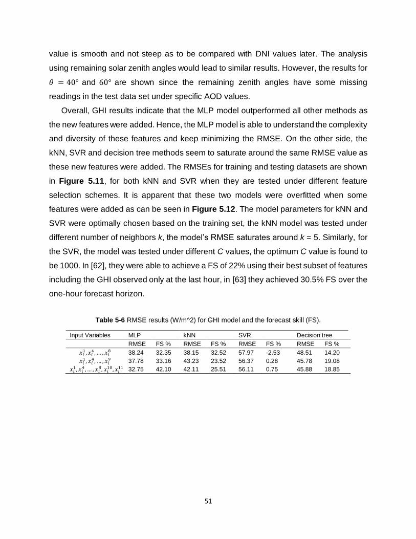
51

value is smooth and not steep as to be compared with DNI values later. The analysis

using remaining solar zenith angles would lead to similar results. However, the results for

𝜃 = 40° and 60° are shown since the remaining zenith angles have some missing

readings in the test data set under specific AOD values.

Overall, GHI results indicate that the MLP model outperformed all other methods as

the new features were added. Hence, the MLP model is able to understand the complexity

and diversity of these features and keep minimizing the RMSE. On the other side, the

kNN, SVR and decision tree methods seem to saturate around the same RMSE value as

these new features were added. The RMSEs for training and testing datasets are shown

in Figure 5.11, for both kNN and SVR when they are tested under different feature

selection schemes. It is apparent that these two models were overfitted when some

features were added as can be seen in Figure 5.12. The model parameters for kNN and

SVR were optimally chosen based on the training set, the kNN model was tested under

different number of neighbors k, the model’s RMSE saturates around k = 5. Similarly, for

the SVR, the model was tested under different C values, the optimum C value is found to

be 1000. In [62], they were able to achieve a FS of 22% using their best subset of features

including the GHI observed only at the last hour, in [63] they achieved 30.5% FS over the

one-hour forecast horizon.

Table 5-6 RMSE results (W/m^2) for GHI model and the forecast skill (FS).

Input Variables MLP kNN SVR Decision tree

RMSE FS % RMSE FS % RMSE FS % RMSE FS %

𝑥𝑖1, 𝑥𝑖

4, … , 𝑥𝑖8 38.24 32.35 38.15 32.52 57.97 -2.53 48.51 14.20

𝑥𝑖1, 𝑥𝑖

4, … , 𝑥𝑖9 37.78 33.16 43.23 23.52 56.37 0.28 45.78 19.08

𝑥𝑖1, 𝑥𝑖

4, … , 𝑥𝑖8, 𝑥𝑖

10, 𝑥𝑖11 32.75 42.10 42.11 25.51 56.11 0.75 45.88 18.85

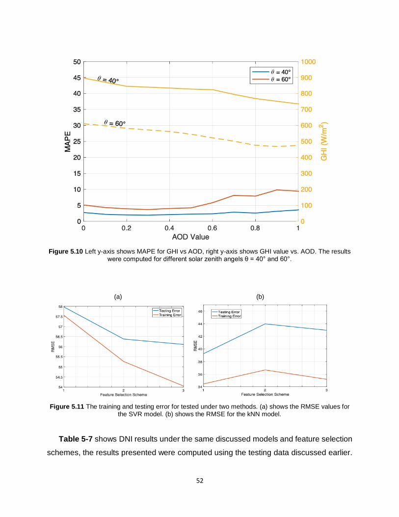
52

Figure 5.10 Left y-axis shows MAPE for GHI vs AOD, right y-axis shows GHI value vs. AOD. The results were computed for different solar zenith angels θ = 40° and 60°.

(a) (b)

Figure 5.11 The training and testing error for tested under two methods. (a) shows the RMSE values for the SVR model. (b) shows the RMSE for the kNN model.

Table 5-7 shows DNI results under the same discussed models and feature selection

schemes, the results presented were computed using the testing data discussed earlier.

53

The parameters of the kNN and SVR models were optimized again for the DNI model

following similar steps discussed earlier for the GHI model. The smart persistence model

for the DNI achieved an RMSE of 102.40 (W/m2). As can be seen from Table 5-7, the

accuracy of all the models kept on improving as more features were added.

In order to analyze this more, the MAPE for DNI is calculated under different 𝐴𝑂𝐷550

values. Figure 5.12 shows the MAPE for DNI versus the 𝐴𝑂𝐷550 value for the model

𝑥𝑖2, 𝑥𝑖

4, … , 𝑥𝑖9

, where the ground observed 𝐴𝑂𝐷550 and angstrom exponent (i.e., 𝑥𝑖10 and

𝑥𝑖11) were not added to the model yet. As before, MAPE for the DNI was measured at two

solar zenith angels 𝜃 = 40° and 60° shown in red and blue in Figure 5.12. As can be

seen from the plots, MAPE for the DNI increases noticeably as the 𝐴𝑂𝐷550 value

increases. Hence, DNI value is very sensitive to 𝐴𝑂𝐷550 value under the clear sky

conditions. The effect of 𝐴𝑂𝐷550 on DNI value is 3 to 4 times larger when compared to

the GHI [64], this can be clearly seen when comparing the GHI and DNI errors in both

Fig. 12 and Figure 5.12 under the same 𝜃. The maximum MAPE for the GHI when 𝜃 =

60° is about 10% while that for the DNI is around 45%. Moreover, the MAPE for DNI also

increases as the solar zenith angle increases (i.e. the beginning and the end of the day).

In [42] they studied multiple AERONET locations around the world and classified the

tested site (i.e. Riyadh, Saudi Arabia) as high turbidity site, moreover, they show that the

AOD versus DNI relationship can be characterized by a linear estimation in low turbidity

sites, however, for high turbidity sites the linear relationship is no longer applicable,

hence, constructing a DNI forecasting model will be a harder problem in these sites. The

yellow lines and the right y-axis in Figure 5.12 show the DNI value under different 𝐴𝑂𝐷550

values, DNI values were computed under two solar zenith angels 𝜃 = 40° and 60°. When

the 𝐴𝑂𝐷550 value increases, a high drop in the DNI values is noticed for the same solar

zenith angle 𝜃.

Now, as the ground measured AERONET 𝐴𝑂𝐷550 𝑥𝑖10and the angstrom exponent 𝑥𝑖

11

were added to the model, a good improvement in the RMSE and FS values was observed

in all of the tested methods, with the MLP having the best RMSE and FS results among

all of the other methods. As can be seen from Table 7, the ground measured AERONET

𝐴𝑂𝐷550 and the angstrom exponent (i.e., 𝑥𝑖10 and 𝑥𝑖

11) acted as a correction factor for the

CAMS 𝐴𝑂𝐷550 (i.e., 𝑥𝑖9) forecasts, hence, the FS for DNI model using MLP has improved

54

by around 8.5% compared to the model where 𝑥𝑖10and𝑥𝑖

11 were not added. The MLP

model had an improvement of around 7.5% compared to the best performing model in

the remaining models (i.e. kNN, SVR and decision tree). The kNN, SVR and decision tree

models had all improved by around 7.28%, 7.3% and 3.34%, respectively, when the new

features (i.e., 𝑥𝑖10 and 𝑥𝑖

11) were added. Overall, a noticeable improvement had been

achieved among all the tested models when the new features (i.e., 𝑥𝑖10and 𝑥𝑖

11) were

added. This is to be expected, since the DNI is very sensitive to 𝐴𝑂𝐷550 values as shown

in Figure 5.12, hence, a more accurate 𝐴𝑂𝐷550 indicators would lead to better performing

DNI forecasting model.

Figure 5.12 Left y-axis shows MAPE for DNI vs AOD, right y-axis shows DNI value vs. AOD. The results were computed at different solar zenith angels θ = 40° and 60°.

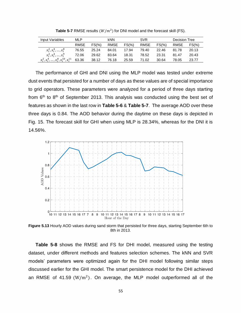
55

Table 5-7 RMSE results (𝑊/𝑚2) for DNI model and the forecast skill (FS).

Input Variables MLP kNN SVR Decision Tree

RMSE FS(%) RMSE FS(%) RMSE FS(%) RMSE FS(%)

𝑥𝑖2, 𝑥𝑖

4, … , 𝑥𝑖8 76.55 25.24 84.01 17.94 79.40 22.46 81.78 20.13

𝑥𝑖2, 𝑥𝑖

4, … , 𝑥𝑖9 72.06 29.62 83.64 18.31 78.52 23.31 81.47 20.43

𝑥𝑖2, 𝑥𝑖

4, … , 𝑥𝑖8, 𝑥𝑖

10, 𝑥𝑖11 63.36 38.12 76.18 25.59 71.02 30.64 78.05 23.77

The performance of GHI and DNI using the MLP model was tested under extreme

dust events that persisted for a number of days as these values are of special importance

to grid operators. These parameters were analyzed for a period of three days starting

from 6th to 8th of September 2013. This analysis was conducted using the best set of

features as shown in the last row in Table 5-6 & Table 5-7. The average AOD over these

three days is 0.84. The AOD behavior during the daytime on these days is depicted in

Fig. 15. The forecast skill for GHI when using MLP is 28.34%, whereas for the DNI it is

14.56%.

Figure 5.13 Hourly AOD values during sand storm that persisted for three days, starting September 6th to 8th in 2013.

Table 5-8 shows the RMSE and FS for DHI model, measured using the testing

dataset, under different methods and features selection schemes. The kNN and SVR

models’ parameters were optimized again for the DHI model following similar steps

discussed earlier for the GHI model. The smart persistence model for the DHI achieved

an RMSE of 41.59 (W/m2) . On average, the MLP model outperformed all of the

56

remaining methods under all feature selection schemes, the decision tree regression had

the second best performance. As more features were added to these models, their RMSE

and FS had improved for all of the tested methods. At first, improvement was observed

when adding the CAMS 𝐴𝑂𝐷550 𝑥𝑖9 in all tested models. As the proposed features (i.e.,

𝑥𝑖10 and 𝑥𝑖

11 ) were added, the overall accuracy has improved significantly across all

models, and slightly for the SVR. For the MLP model, the FS has improved by around

13.4% when compared to the model that utilizes the CAMS 𝐴𝑂𝐷550. Similarly, FS has

improved by around 7% for the kNN, 4.5% for SVR and 12.5% for decision tree. As for

the GHI and DNI models implemented earlier, the MLP model has shown a superior

accuracy when compared to the other methods, moreover, the proposed features (i.e.,

𝑥𝑖10and 𝑥𝑖

11) increased the accuracy noticeably across all the tested methods.

Table 5-8 RMSE results (W/m^2) for DHI model and the forecast skill (FS).

Input Variables MLP kNN SVR Decision Tree

RMSE FS(%) RMSE FS(%) RMSE FS(%) RMSE FS(%)

𝑥𝑖3, 𝑥𝑖

4, … , 𝑥𝑖8 31.00 25.45 35.66 14.25 37.89 8.9 36.36 12.56

𝑥𝑖3, 𝑥𝑖

4, … , 𝑥𝑖9 29.47 29.13 33.81 18.68 36.88 11.31 35.98 13.48

𝑥𝑖3, 𝑥𝑖

4, … , 𝑥𝑖8, 𝑥𝑖

10, 𝑥𝑖11 23.90 42.52 30.88 25.73 35.02 15.78 30.79 25.96

Further analysis for the DHI performance versus the 𝐴𝑂𝐷550 value is shown in Figure

5.14. The MAPE for DHI decreases as the 𝐴𝑂𝐷550 value increases. The MAPE is

relatively small when compared to the MAPE for DNI model under the same solar zenith

angle. For example, when 𝜃 = 60°, the maximum MAPE for the DHI model is about 15%,

while for the DNI model it’s is about 45%. As with the previous models, the MAPE for DHI

increases as the solar zenith angle increases (i.e. at the beginning and the end of the

day). The DHI readings were also compared with the 𝐴𝑂𝐷550 values in Figure 5.14 as

shown in yellow lines and the right y-axis. As can be clearly seen, the DHI readings

increase as the 𝐴𝑂𝐷550 value increases. This is mainly because of the radiation scattering

caused by the 𝐴𝑂𝐷550 particles in the air. Overall, a significant improvement has be

achieved when the new features were added to the model, that’s due to the fact that DHI

is moderately sensitive to 𝐴𝑂𝐷550 as shown in Fig. 16. Hence, feeding the tested models

with the new set of features (i.e., 𝑥𝑖10and 𝑥𝑖

11), would lead to an improved accuracy for the

DHI forecasting model across all the implemented methods. Figure 5.15 shows the MLP

57

model sensitivity for (GHI/DNI/DHI) under different AOD values. As can be seen from the

figure and as discussed earlier in Figure 5.9, the DNI is the most sensitive radiation

variable to dust; DHI is less sensitive to dust when compared to DNI; and GHI is the least

sensitive to dust.

Figure 5.14 Left y-axis shows MAPE for DHI vs AOD, right y-axis shows DHI value vs. AOD. The results were computed at different solar zenith angels θ = 40° and 60°.

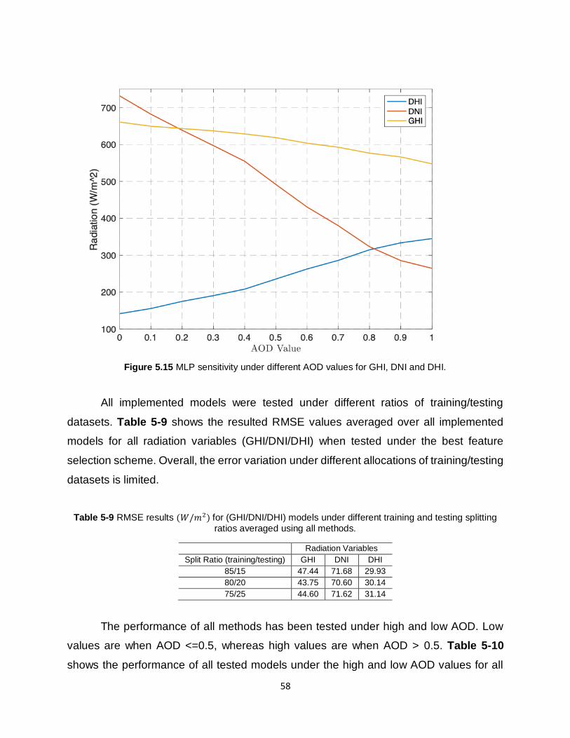
58

Figure 5.15 MLP sensitivity under different AOD values for GHI, DNI and DHI.

All implemented models were tested under different ratios of training/testing

datasets. Table 5-9 shows the resulted RMSE values averaged over all implemented

models for all radiation variables (GHI/DNI/DHI) when tested under the best feature

selection scheme. Overall, the error variation under different allocations of training/testing

datasets is limited.

Table 5-9 RMSE results (𝑊/𝑚2) for (GHI/DNI/DHI) models under different training and testing splitting

ratios averaged using all methods.

Radiation Variables

Split Ratio (training/testing) GHI DNI DHI

85/15 47.44 71.68 29.93

80/20 43.75 70.60 30.14

75/25 44.60 71.62 31.14

The performance of all methods has been tested under high and low AOD. Low

values are when AOD <=0.5, whereas high values are when AOD > 0.5. Table 5-10

shows the performance of all tested models under the high and low AOD values for all

59

radiation variables (GHI/DNI/DHI). As shown, MLP has the best performance among all

methods under all radiation variables, for both the high and low AOD value cases. As can

be seen from results, the accuracy of all methods decreases when AOD values are high.

Figure 5.16 shows the MAPE performance for (GHI/DNI/DHI) for each month of the year.

MAPE has a slight increase for high AOD months for both GHI and DNI, whereas for DHI

the MAPE decreases during these months. The models’ performance has been analyzed

for periods with above average variability values. The average and standard deviation for

these inputs are shown in Table 5-5. Only periods with at least 10% standard deviation

values above the average were tested. The variables that were considered are the

variables that change inconsistently over the day, these variables are the AOD, wind

speed, wind direction. Table 5-11 shows the performance of the different radiation

variables across all the models when tested under high variability periods. As can be seen

from Table 5-11, the MLP and Decision Tree models are the most robust models during

high variability periods.

Table 5-10 RMSE results (𝑊/𝑚2) for all methods under low and high AOD values.

Radiation Variables

AOD Range Method

MLP kNN SVR Decision

Tree

GHI AOD<=0.5 25.28 31.90 52.42 41.72

AOD>0.5 43.43 56.47 66.46 59.52

DNI AOD<=0.5 51.43 65.86 67.49 74.13

AOD>0.5 67.27 90.46 73.77 81.19

DHI AOD<=0.5 21.25 26.49 35.37 25.72

AOD>0.5 27.97 36.92 35.99 39.37

60

Figure 5.16 MAPE Averaged over all methods for each month of the year.

Table 5-11 RMSE results (𝑊/𝑚2) for all methods during high variability periods.

Method Radiation Variables

GHI DNI DHI

MLP 25.76 39.72 20.74

kNN 39.29 48.24 23.92

SVR 45.07 53.83 27.88

Decision Tree 20.98 37.78 18.10

61

Chapter 6 Case Study

In this chapter the main case study is presented. The chapter is divided into three

main section. In the first section, the internal architecture of the neural networks were

tested under different number of neurons for each hidden layer, to investigate what would

be the best internal NN architecture for each of the forecasted variables (i.e. PV panel

system, mosque, clinic and office building).

In the second section, the different combination of input features (shown in Table

3-1 and Table 3-2) were tested for each of the forecasted variables, these tested models

were also tested under four different forecasting techniques as discussed in the

Methodology chapter. The total number of the test cases is 124 models for each one of

the forecasted variables, a total of 496 test cases for all of the four forecasted variables.

The third section in this chapter investigates the total savings achieved when

implementing the proposed forecasting model combined with the CTES (shown in Figure

1.1 and Figure 3.1), the test cases include different chiller and CTES capacity values.

6.1 Neural Networks Internal Architecture Results

As discussed earlier, the implemented neural networks method in this work is the

feedforward network. In order to find the best architecture for each forecasted variable

(i.e. PV panel system, mosque, clinic and office building), each one of these forecasted

variables was tested under different internal NN architectures. The meaning of

architecture in this context is the number of neurons in each hidden layer in the NN, while

the internal neurons between each two consecutive layers are fully connected. Each

forecasted variable has been tested under three hidden layers and a different number of

neurons on each layer, then the best architecture was chosen for each forecasted

variable. All the forecasted variables were tested under the feature selection scheme

labelled as 31 in Table 3-2. This feature combination was chosen as it represents the

most complex set of features when compared to the other sets of features, even though

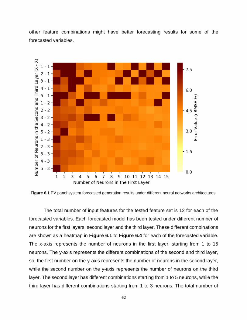
62

other feature combinations might have better forecasting results for some of the

forecasted variables.

Figure 6.1 PV panel system forecasted generation results under different neural networks architectures.

The total number of input features for the tested feature set is 12 for each of the

forecasted variables. Each forecasted model has been tested under different number of

neurons for the first layers, second layer and the third layer. These different combinations

are shown as a heatmap in Figure 6.1 to Figure 6.4 for each of the forecasted variable.

The x-axis represents the number of neurons in the first layer, starting from 1 to 15

neurons. The y-axis represents the different combinations of the second and third layer,

so, the first number on the y-axis represents the number of neurons in the second layer,

while the second number on the y-axis represents the number of neurons on the third

layer. The second layer has different combinations starting from 1 to 5 neurons, while the

third layer has different combinations starting from 1 to 3 neurons. The total number of

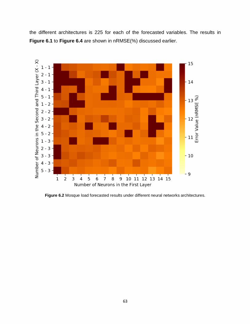
63

the different architectures is 225 for each of the forecasted variables. The results in

Figure 6.1 to Figure 6.4 are shown in nRMSE(%) discussed earlier.

Figure 6.2 Mosque load forecasted results under different neural networks architectures.

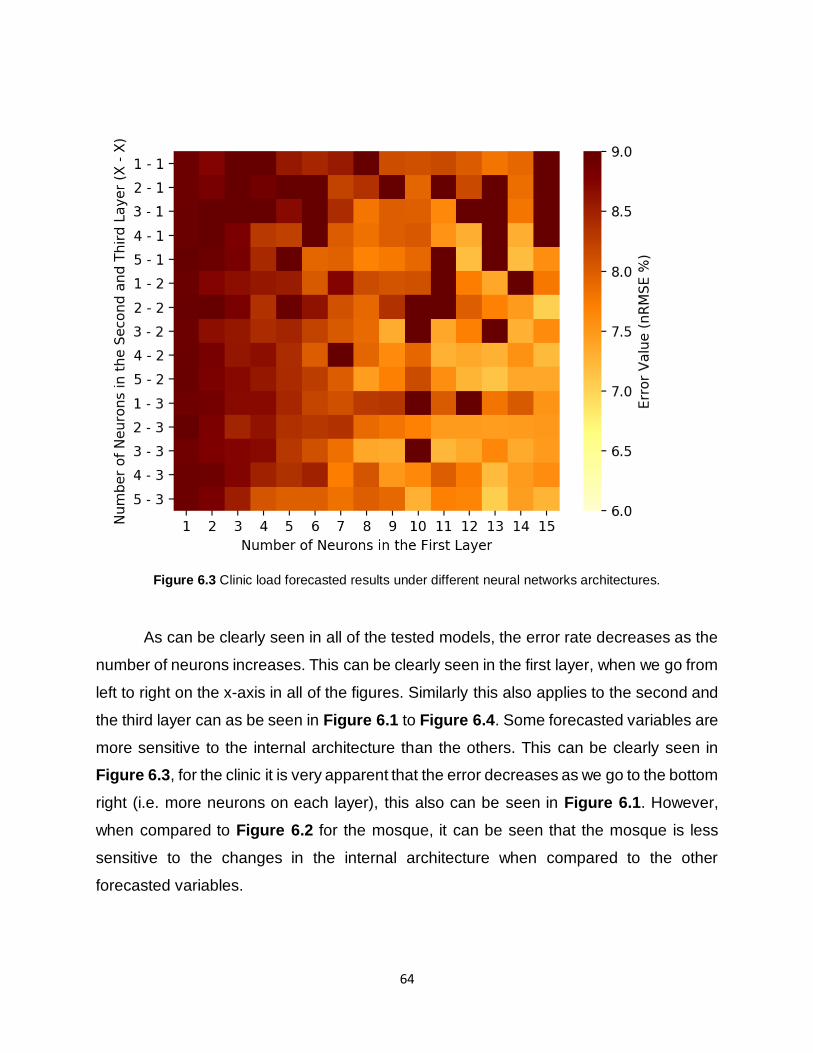
64

Figure 6.3 Clinic load forecasted results under different neural networks architectures.

As can be clearly seen in all of the tested models, the error rate decreases as the

number of neurons increases. This can be clearly seen in the first layer, when we go from

left to right on the x-axis in all of the figures. Similarly this also applies to the second and

the third layer can as be seen in Figure 6.1 to Figure 6.4. Some forecasted variables are

more sensitive to the internal architecture than the others. This can be clearly seen in

Figure 6.3, for the clinic it is very apparent that the error decreases as we go to the bottom

right (i.e. more neurons on each layer), this also can be seen in Figure 6.1. However,

when compared to Figure 6.2 for the mosque, it can be seen that the mosque is less

sensitive to the changes in the internal architecture when compared to the other

forecasted variables.

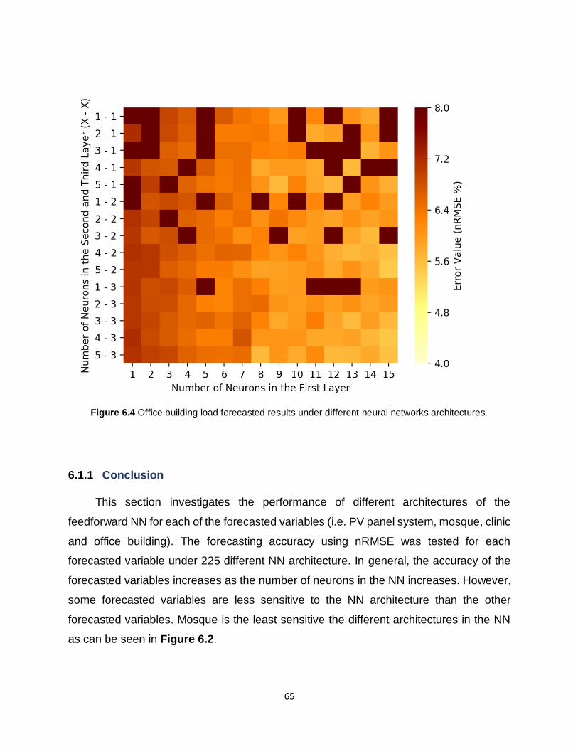
65

Figure 6.4 Office building load forecasted results under different neural networks architectures.

6.1.1 Conclusion

This section investigates the performance of different architectures of the

feedforward NN for each of the forecasted variables (i.e. PV panel system, mosque, clinic

and office building). The forecasting accuracy using nRMSE was tested for each

forecasted variable under 225 different NN architecture. In general, the accuracy of the

forecasted variables increases as the number of neurons in the NN increases. However,

some forecasted variables are less sensitive to the NN architecture than the other

forecasted variables. Mosque is the least sensitive the different architectures in the NN

as can be seen in Figure 6.2.

66

6.2 Forecasting Results

6.2.1 PV panel results

The PV panel forecasting results are shown in Figure 6.5, each row in the heat

map refers to a feature combination as shown in Table 3-2, each column refers to a

forecasting method as described in earlier. The first 16 feature refer to individual feature

selection combination, meaning that, only one variable was used to build and test the that

specific forecasting model. The remaining features are different combinations of these

individual features. The best individual feature when performing the PV panel power

forecasts is the 𝑥𝑖ℎ𝑖𝑠𝑡𝑜𝑟𝑖𝑐𝑎𝑙 which is 𝑥𝑖

18 when doing forecasting for the PV panels. The best

results for the model are shown in Table 6-1 under different error metrics, this was

achieved using the SVR model, when using the set of features as indicated by number

30 in Table 3-2. The set of features include the forecasted GHI, DNI, time and date

variables, high cloud cover, dust AOD, wind speed, wind direction and the previous day

PV power generation at the same hour. The individual features 1,2,3,4,13 and 19 have

good results when they are used alone without combining them with other features. These

features are the clear sky GHI, clear sky DNI, forecasted GHI, forecasted DNI, the hour

of the day and the previous day PV power generation. That’s expected when building a

forecasting model for the PV panels, as these features contribute more to the output

power of the PV panels when compared with the other features. It is also worth noting

that the remaining individual features have a big error gap compared to these 5 best

individual features. This gap in the error is also present when comparing these individual

features with the remaining different combinations of the features. The weakest model

occurs when using the wind speed and the wind direction alone as inputs without using

other input features under the kNN forecasting model.

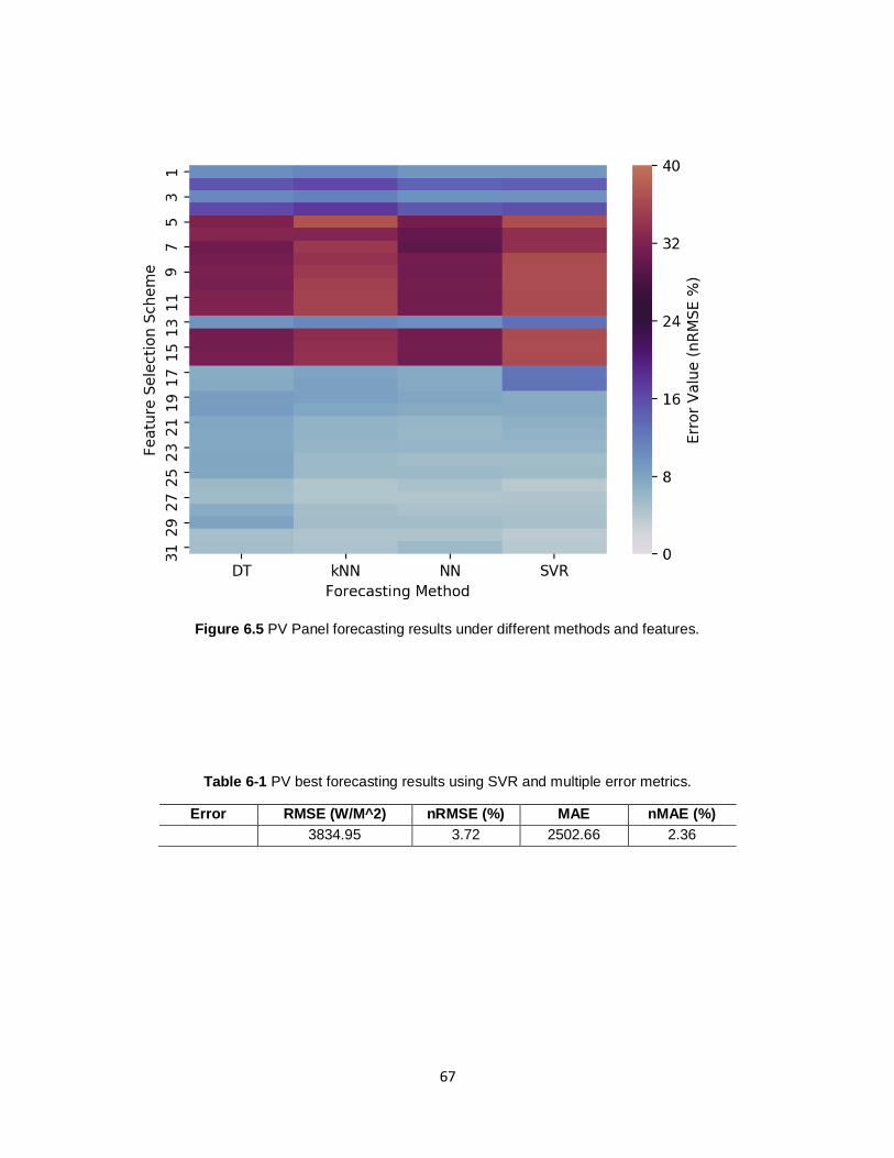
67

Figure 6.5 PV Panel forecasting results under different methods and features.

Table 6-1 PV best forecasting results using SVR and multiple error metrics.

Error

Metric

RMSE (W/M^2) nRMSE (%) MAE nMAE (%)

3834.95 3.72 2502.66 2.36

68

6.2.2 Buildings Load results

Similarly, as the PV forecasts, all the building types were tested under different

features combinations as shown in Table 3-2. The following subsections will discuss the

forecasting results for each of these building types (i.e. mosque, clinic and office building)

6.2.3 Mosque

The mosque forecasting results tested under different forecasting methods and

feature selections schemes are shown in the heatmap in Figure 6.6. The different feature

combinations were discussed earlier in Table 3-2. The top individual features in terms of

accuracy when building the forecasting model are two features, the hour of the day and

the previous week power consumption for the mosque at the same hour, this can be

clearly seen in the heatmap as features 13 and 19. Unlike the PV forecasts, the individual

features have a lower error gap when compared to the combined feature combinations.

When compared to the other forecasted variables (i.e. PV panel system, clinic and office

building), the mosque is the hardest to forecast, this can be seen in the relatively high

error rate when compared with the other forecasted variables. This relatively high error

rate is because of the high variability in the load profile of the mosque, meaning that the

mosque has 5 different peaks, these 5 load peaks are dependent on the solar time and

less on the hour of the day. The high error in the mosque is also caused by the

unpredictability of the cooling load, as the number of people attended the prayers is

varied, hence, this causes an increase in the variability of the cooling load. The load profile

of the mosque is also dependent on the on the weekday and weekend schedule, that’s

because on Friday noon the Jumaa prayer takes place. Moreover, the mosque is usually

crowded during the weekend, as people pray in the mosque instead of their working place.

The best model when building a forecasting was achieved when applying the kNN under

the feature combination numbered as 29 in Table 3-2. The set of features for this model

include the temperature, previous week power consumption at the same hour, hour of the

day, month of the year, the day of the year, cloud cover and the dust AOD information.

The kNN model results are shown in Table 6-2 under different error metrics. It can be

seen from Table 6-2 that the gap in the error between the RMSE and the MAE is relatively

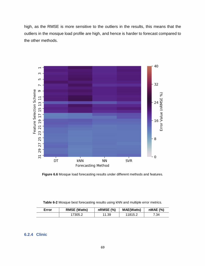
69

high, as the RMSE is more sensitive to the outliers in the results, this means that the

outliers in the mosque load profile are high, and hence is harder to forecast compared to

the other methods.

Figure 6.6 Mosque load forecasting results under different methods and features.

Table 6-2 Mosque best forecasting results using kNN and multiple error metrics.

Error

Metric

RMSE (Watts) nRMSE (%) MAE(Watts) nMAE (%)

17305.2 11.39 11815.2 7.34

6.2.4 Clinic

70

The clinic forecasting results tested under different forecasting methods and

feature selections schemes are shown in the heatmap in Figure 6.7. The different feature

combinations were discussed earlier in Table 3-2. The top individual features in terms of

accuracy when building the forecasting model for the clinic are three features, the

temperature, the previous week power consumption for the clinic at the same hour and

the month of the year, this can be clearly seen in the heatmap as features 7, 14 and 19.

Similar to the mosque forecasting models, the individual features have a lower error gap

when compared to the combined feature combinations, unlike the PV panels shown in

Figure 6.5. Also, the error gap between the best and worst model in the clinic models is

narrower than the gap in the mosque results, meaning that the features in Table 3-1 have

weights close to each other when building the forecasting model for the clinic. Also it

means that the clinic load profile is smoother than the mosque load profile as shown

earlier in Figure 4.2, so, as the load profile gets smoother the effect of the input features

decrease as we reach to straight line, at that point the input feature has no effect on the

model output, and the output of the model is the same regardless of the input feature.

When compared to the other forecasted variables (i.e. PV panel system, clinic and office

building), the clinic has the smoothest load profile, so the gap between the maximum ad

the minimum load is the smallest among all the other forecasted variables. The load

profile of the clinic is also dependent on the on the weekday and weekend schedule. The

best model when building a forecasting was achieved when applying the SVR under the

feature combination numbered as 30 in Table 3-2. The set of features for this model

include the temperature, previous week power consumption at the same hour, hour of the

day, month of the year, the day of the year, cloud cover, the wind data, GHI alongside

with the dust AOD information. The SVR model results are shown in Table 6-3 under

different error metrics. It can be seen from Table 6-3 that the gap in the error between

the RMSE and the MAE is relatively small as when compared to the mosque gap, as the

RMSE is more sensitive to the outliers in the results, this means that the outliers in the

clinic load profile are small when compared to the mosque, and hence is easier to forecast

compared to mosque.

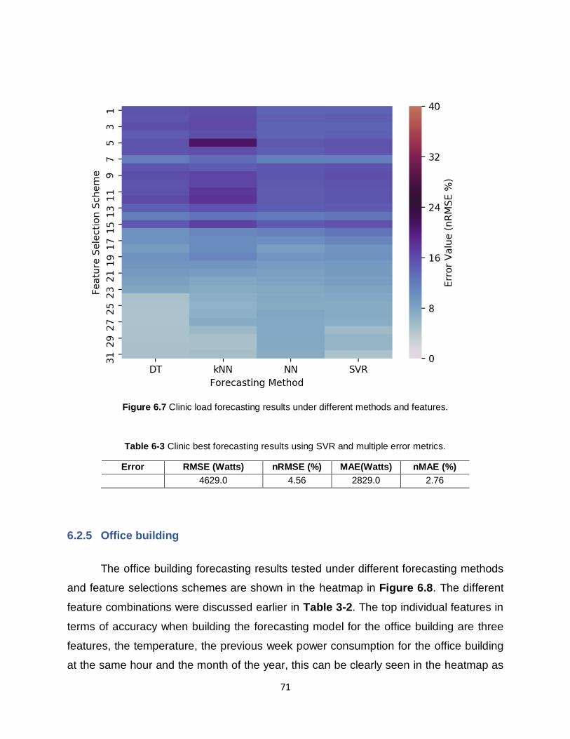
71

Figure 6.7 Clinic load forecasting results under different methods and features.

Table 6-3 Clinic best forecasting results using SVR and multiple error metrics.

Error

Metric


4629.0 4.56 2829.0 2.76

6.2.5 Office building

The office building forecasting results tested under different forecasting methods

and feature selections schemes are shown in the heatmap in Figure 6.8. The different

feature combinations were discussed earlier in Table 3-2. The top individual features in

terms of accuracy when building the forecasting model for the office building are three

features, the temperature, the previous week power consumption for the office building

at the same hour and the month of the year, this can be clearly seen in the heatmap as

72

features 7, 14 and 19, these top features are similar to the top features for the clinic

forecasting model. Also, as the mosque and the clinic forecasting models, the individual

features have a lower error gap when compared to the combined feature combinations,

unlike the PV panels shown in Figure 6.5. Also, the error gap between the best and worst

model in the office building models is narrower than the gap in the mosque and clinic

results, meaning that the features in Table 3-1 have weights close to each other when

building the forecasting model for the office building. The load profile of the office building

is similar to the mosque and the clinic, as it also dependent on the on the weekday and

weekend schedule. The best model when building a forecasting was achieved when

applying the SVR under the feature combination numbered as 30 in Table 3-2. The set

of features for this model include the temperature, previous week power consumption at

the same hour, hour of the day, month of the year, the day of the year, cloud cover, the

wind data, GHI alongside with the dust AOD information. The best set of features are

similar to the best set of features for the clinic. The SVR model results are shown in Table

6-4 under different error metrics. It can be seen from Table 6-4 that the gap in the error

between the RMSE and the MAE is relatively small as when compared to the mosque

gap, as the RMSE is more sensitive to the outliers in the results, this means that the

outliers in the office building load profile are small when compared to the mosque, and

hence is easier to forecast compared to mosque. Moreover, this gap is smaller in the

office building when compared with the clinic as well, as the gap between nRMSE and

nMAE is 1.79% in the clinic, while in the office building this gap is only 1.25%. Meaning

that the outliers in the building results are the lowest among all the other forecasted

variables. This can be seen also in the results, as the office building has the lowest error

when compared to the remaining forecasted variables (i.e. PV panel system, mosque and

clinic).

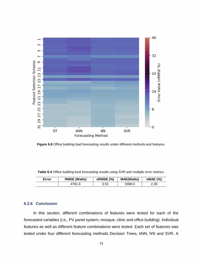
73

Figure 6.8 Office building load forecasting results under different methods and features.

Table 6-4 Office building best forecasting results using SVR and multiple error metrics.

Error

Metric


4761.6 3.53 3368.0 2.28

6.2.6 Conclusion

In this section, different combinations of features were tested for each of the

forecasted variables (i.e., PV panel system, mosque, clinic and office building). Individual

features as well as different feature combinations were tested. Each set of features was

tested under four different forecasting methods Decision Trees, kNN, NN and SVR. A

74

total of 124 test cases were conducted for each forecasted variable. nRMSE of 3.73%,

11.39%, 4.56% and 3.53% were achieved for the PV panel system, mosque, clinic and

the office building, respectively.

6.3 Total savings using the proposed method

In this section the total savings is discussed by comparing the proposed method

with the baseline model. The proposed method is where building-level load forecasts and

PV forecasts are taken into account to determine CTES charge schedule for the next day.

The baseline model is where the CTES charge for tomorrow is scheduled to be fully

charged to cover loads of the entire district.

The baseline and the proposed system were tested under different scenarios. The

first test case includes changing the maximum chiller capacity that met the cooling load.

Any cooling load that exceeds the maximum chiller capacity is met using the CTES

charge. As described earlier, the CTES charge for the baseline system is fully charged

during the night regardless of the total cooling demand for tomorrow. On the other side,

the proposed system is charged based on the total forecasted load plus the error factor,

which was chosen to be close to the worst forecasting error, which is around 10%. The

total cooling load is forecasted from 07:00 a.m. to 05:00 p.m., the CTES is charged based

on the demand during this period plus 10% of the total forecasted load. Both the baseline

and the forecasting systems were tested under different maximum chiller capacity

scenarios, as discussed below.

6.3.1 Systems tested under different chiller values

In this section, the baseline system and the forecasting system were both tested

under different chiller capacity values.

6.3.1.1 180 kW maximum chiller capacity

75

6.3.1.1.1 Baseline method

In this test case, the maximum chiller capacity is 180 kW, while the peak cooling

load is 219,16 kW at 01:00 p.m., taking into consideration that the load is forward

averaged as described earlier in the data section. Figure 6.9 shows the overall system

under the baseline method. The CTES is charged during the night from 12:00 a.m. to

06:00 am., then during the day, the CTES charge is discharged when the cooling load

exceeds the chiller capacity. And finally, any charge that’s remaining after 05:00 p.m. is

calculated. As can be seen from the plot, the CTES is being charged during the night at

a steady rate until 06:00 a.m., after that, the CTES stopped charging and in standby

mode. As can be seen from the plot, the standby mode is active at 07:00 a.m., as the

maximum cooling load is around 156 kW, which is less than the maximum chiller capacity.

Hence, the cooling load is met using only the chiller, and the CTES charge is preserved

for the upcoming hours. Now, at 08:00 a.m., the total cooling load starts increasing, and

the load is 191 kW, which is higher that the maximum capacity. Hence, the total cooling

load must be met using both the maximum chiller capacity and the preserved charge in

the CTES. As can be seen at 08:00 the CTES charge starts decreasing at a rate equal to

the difference between the load and the maximum chiller capacity, which is around 10

kWh at 08:00 a.m.. The system starts discharging during the subsequent hours as can

be seen in the plot. The maximum discharge rate occurs at 01:00 p.m., as the maximum

cooling load is around 220 kW, hence, the difference between the cooling load and the

maximum chiller capacity is 20 kWh. The discharge rate starts decreasing after 01:00

p.m. as shown in the plot. After 05:00 p.m. there is still a remaining charge in the CTES

that has not been fully utilized yet, the remaining charge in the CTES is equal to 64 kWh

when applying the baseline method.

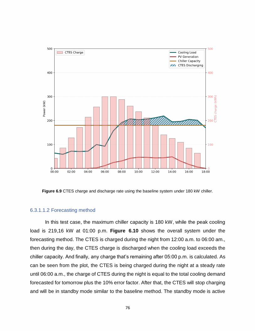
76

Figure 6.9 CTES charge and discharge rate using the baseline system under 180 kW chiller.

6.3.1.1.2 Forecasting method

In this test case, the maximum chiller capacity is 180 kW, while the peak cooling

load is 219,16 kW at 01:00 p.m. Figure 6.10 shows the overall system under the

forecasting method. The CTES is charged during the night from 12:00 a.m. to 06:00 am.,

then during the day, the CTES charge is discharged when the cooling load exceeds the

chiller capacity. And finally, any charge that’s remaining after 05:00 p.m. is calculated. As

can be seen from the plot, the CTES is being charged during the night at a steady rate

until 06:00 a.m., the charge of CTES during the night is equal to the total cooling demand

forecasted for tomorrow plus the 10% error factor. After that, the CTES will stop charging

and will be in standby mode similar to the baseline method. The standby mode is active

77

during 07:00 a.m., while the total cooling load is around 156 kW, which is less than the

maximum chiller capacity. Hence, the cooling load is met only using only the chiller, and

the CTES charge is preserved for the upcoming hours. Now, at 08:00 a.m., the total

cooling load starts increasing, and the load is 191 kW, which is higher than the maximum

capacity. Hence, the total cooling load must be met using both the maximum chiller

capacity and the preserved charge in the CTES. As can be seen at 08:00 the CTES

charge starts decreasing at a rate equal to the difference between the load minus the

maximum chiller capacity, which is around 10 kWh at 08:00 a.m.. The system starts

discharging in the subsequent hours as can be seen in the plot. The maximum discharge

rate occurs at 01:00 p.m. The discharge rate starts decreasing after 01:00 p.m. as shown

in the plot. After 05:00 p.m. there is still a remaining charge in the CTES that has not been

fully utilized yet, the remaining charge in the CTES is equal to 23 kWh when applying the

forecasting method.

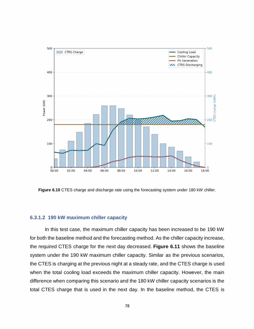
78

Figure 6.10 CTES charge and discharge rate using the forecasting system under 180 kW chiller.


In this test case, the maximum chiller capacity has been increased to be 190 kW

for both the baseline method and the forecasting method. As the chiller capacity increase,

the required CTES charge for the next day decreased. Figure 6.11 shows the baseline

system under the 190 kW maximum chiller capacity. Similar as the previous scenarios,

the CTES is charging at the previous night at a steady rate, and the CTES charge is used

when the total cooling load exceeds the maximum chiller capacity. However, the main

difference when comparing this scenario and the 180 kW chiller capacity scenarios is the

total CTES charge that is used in the next day. In the baseline method, the CTES is

79

charged fully during the night regardless of the required CTES charge. As can be seen

from the plot, the CTES charge is used starting at 08:00 a.m., similar to the previous

scenario. However, in this scenario, the discharge rate at 08:00 is lower, as the total

cooling load is 191 kW and the maximum chiller capacity is 190 kW, hence, the required

discharge is only 1 kWh. This also applies to the subsequent hours. The CTES is

discharging until 05:00 p.m., similar to the previous scenario. However, the remaining

charge in the CTES is higher in this case, as the CTES discharge rate is lower during the

peak hours. The remaining charge in the CTES at 05:00 p.m. is 164 kWh, which is much

higher than the previous case.


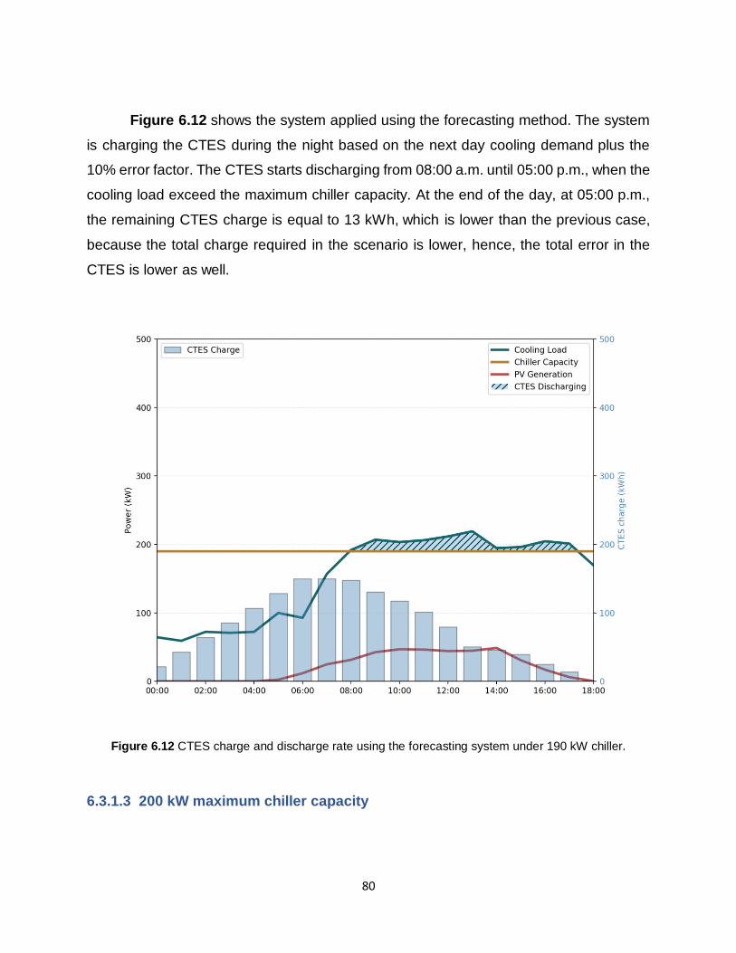
80

Figure 6.12 shows the system applied using the forecasting method. The system

is charging the CTES during the night based on the next day cooling demand plus the

10% error factor. The CTES starts discharging from 08:00 a.m. until 05:00 p.m., when the

cooling load exceed the maximum chiller capacity. At the end of the day, at 05:00 p.m.,

the remaining CTES charge is equal to 13 kWh, which is lower than the previous case,

because the total charge required in the scenario is lower, hence, the total error in the

CTES is lower as well.



81

In this test case, the maximum chiller capacity has been increased to be 200 kW

for both the baseline method and the forecasting method. Similar to the previous scenario,

since the chiller capacity has increased, the required CTES charge for the next day has

also decreased. Figure 6.13 shows the baseline system under the 200 kW maximum

chiller capacity. Similar as the previous scenarios, the CTES is charging at the previous

night at a steady rate, and the CTES charge is used when the total cooling load exceeds

the maximum chiller capacity. However, the main difference when comparing this

scenario and the previous scenarios, is that in this case the CTES charge is used in two

separate periods of the day, meaning that, the CTES started discharging when the cooling

load exceeds the chiller capacity at 09:00 a.m., and stopped discharging at 02:00 p.m.,

when there is a drop in the load. Then again, the CTES started discharging at 04:00 p.m.

In this scenario, the discharge rate at all hours is lower than the previous scenarios, since

the chiller capacity is lower, hence, the required charge from the CTES is also lower. The

remaining charge in the CTES is higher in this case than the previous cases. The

remaining charge in the CTES at 05:00 p.m. is 246 kWh, which is higher than the previous

cases.

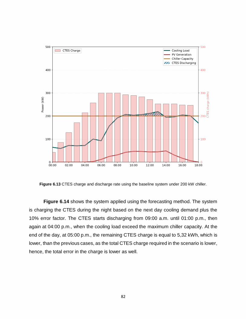
82


Figure 6.14 shows the system applied using the forecasting method. The system

is charging the CTES during the night based on the next day cooling demand plus the

10% error factor. The CTES starts discharging from 09:00 a.m. until 01:00 p.m., then

again at 04:00 p.m., when the cooling load exceed the maximum chiller capacity. At the

end of the day, at 05:00 p.m., the remaining CTES charge is equal to 5,32 kWh, which is

lower, than the previous cases, as the total CTES charge required in the scenario is lower,

hence, the total error in the charge is lower as well.

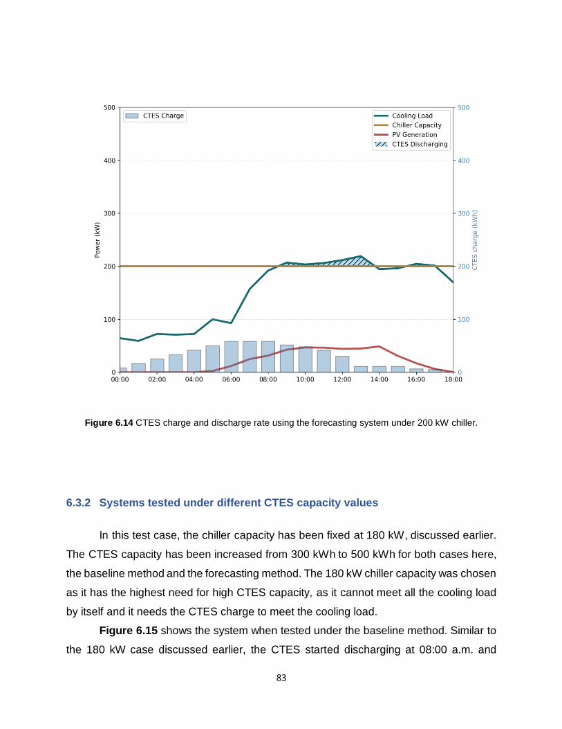
83


6.3.2 Systems tested under different CTES capacity values

In this test case, the chiller capacity has been fixed at 180 kW, discussed earlier.

The CTES capacity has been increased from 300 kWh to 500 kWh for both cases here,

the baseline method and the forecasting method. The 180 kW chiller capacity was chosen

as it has the highest need for high CTES capacity, as it cannot meet all the cooling load

by itself and it needs the CTES charge to meet the cooling load.

Figure 6.15 shows the system when tested under the baseline method. Similar to

the 180 kW case discussed earlier, the CTES started discharging at 08:00 a.m. and

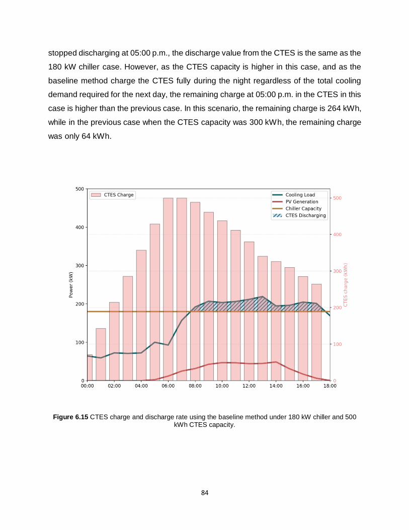
84

stopped discharging at 05:00 p.m., the discharge value from the CTES is the same as the

180 kW chiller case. However, as the CTES capacity is higher in this case, and as the

baseline method charge the CTES fully during the night regardless of the total cooling

demand required for the next day, the remaining charge at 05:00 p.m. in the CTES in this

case is higher than the previous case. In this scenario, the remaining charge is 264 kWh,

while in the previous case when the CTES capacity was 300 kWh, the remaining charge

was only 64 kWh.

Figure 6.15 CTES charge and discharge rate using the baseline method under 180 kW chiller and 500 kWh CTES capacity.

85

Figure 6.16 shows system tested under the 500 kWh CTES capacity using the

forecasting method. The required CTES charge during the day in order to meet the

cooling load is the same as the baseline method. However, the main difference is the

percentage of CTES that was charged during the night. In this case the forecasted cooling

load plus the 10% error factor was charged during the night. At 05:00 p.m. the remaining

charge is 23 kWh in the CTES, same as the case when the CTES capacity was 300 kWh

and tested under the forecasting method. Meaning that the forecasting method is

independent of the CTES capacity and is only charged based on the required load for the

next day. However, the difference in the charge in the 300 kWh and 500 kWh chiller

capacity between the baseline and the forecasting method has increased. In the 300 kWh

case the difference was only 41 kWh, while in the 500 kWh case, the difference increased

to 241 kWh. As can be seen in this case, the forecasting method is more desirable when

the CTES capacity increases. Because the remaining charge in the CTES when using

the baseline method increased with the CTES capacity.

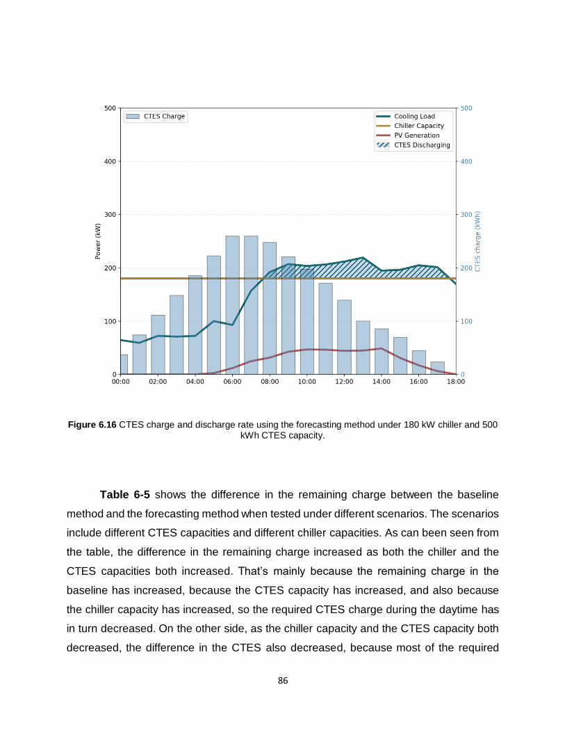
86

Figure 6.16 CTES charge and discharge rate using the forecasting method under 180 kW chiller and 500 kWh CTES capacity.

Table 6-5 shows the difference in the remaining charge between the baseline

method and the forecasting method when tested under different scenarios. The scenarios

include different CTES capacities and different chiller capacities. As can been seen from

the table, the difference in the remaining charge increased as both the chiller and the

CTES capacities both increased. That’s mainly because the remaining charge in the

baseline has increased, because the CTES capacity has increased, and also because

the chiller capacity has increased, so the required CTES charge during the daytime has

in turn decreased. On the other side, as the chiller capacity and the CTES capacity both

decreased, the difference in the CTES also decreased, because most of the required

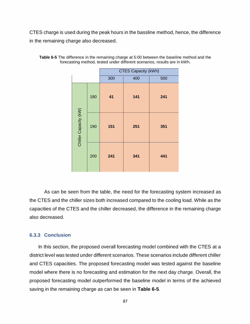
87

CTES charge is used during the peak hours in the bassline method, hence, the difference

in the remaining charge also decreased.

Table 6-5 The difference in the remaining charge at 5:00 between the baseline method and the forecasting method, tested under different scenarios, results are in kWh.

CTES Capacity (kWh)

300 400 500

180 41 141 241

190 151 251 351

200 241 341 441

As can be seen from the table, the need for the forecasting system increased as

the CTES and the chiller sizes both increased compared to the cooling load. While as the

capacities of the CTES and the chiller decreased, the difference in the remaining charge

also decreased.

6.3.3 Conclusion

In this section, the proposed overall forecasting model combined with the CTES at a

district level was tested under different scenarios. These scenarios include different chiller

and CTES capacities. The proposed forecasting model was tested against the baseline

model where there is no forecasting and estimation for the next day charge. Overall, the

proposed forecasting model outperformed the baseline model in terms of the achieved

saving in the remaining charge as can be seen in Table 6-5.

Chill

er

Capacity (

kW

)

88

Chapter 7 Conclusion and Future

Work

7.1 Conclusion

In hot countries cooling systems consume a large portion of buildings’ overall load.

Moreover, these cooling systems are only fully utilized during the peak demand hours in

a few very hot summer days. These large cooling systems increase the capital investment

needed at the installation phase. CTES is a good option to lower these initial costs

associated with the installation of large cooling systems, as the required cooling systems

in this case has a lower peak capacity, hence, a lower price. A shared cooling system

and CTES at a district level would allow for a better utilization of these resources. The

integration of the shared cooling system with CTES at a district level improve the

utilization of the cooling system, by lowering the peak of the cooling demand, hence, the

cooling system is better utilized during the year.

In this dissertation a solution was presented to avoid creating a building peak

demand, using Cool Thermal Energy Storage (CTES) deployed at a district level

combined with PV and building load forecasting. It also answered one important question

- how much of the CTES should be charged during the night, such that the cooling load

for the next day is fully met and at the same time the CTES charge is fully utilized during

the day.

The solution presented in this dissertation integrated the CTES with PV power

forecasting and building load forecasting at district level for its better charge/discharge

management. A district comprises several buildings of different load profiles, namely,

mosque, clinic and the office building. All of these buildings are connected to the same

cooling system and a shared CTES. The use of the forecasting for both the PV and the

building cooling load allows the building operator to more accurately determine how much

of the CTES should be charged during the night, in order to meet the cooling peak

89

demand of the next day. Using this approach, the charge of the CTES is utilized more

efficiently during the day, also saving is achieved in the capital costs during the initial

installation of the cooling capacity, as well as savings for the utility company by lowering

their peak load.

The district presented in this dissertation has PV panel system and three types of

buildings, mosque, clinic and office building. In order to have a good estimation for the

required CTES charge for the next day, good forecasts for the PV panel system and the

building load would be required. In this presented work, the dust was introduced as a new

input feature in all of the forecasting models to improve the models’ accuracy. Dust is an

important input feature for the forecasts in areas with high dust values. All the forecasts

were tested under four machine learning forecasting methods, namely Decision Trees, k-

Nearest Neighbor, Neural Networks and Support Vector Regression. Each forecasting

method was tested under 31 feature combinations to investigate which set of features are

best for each forecasting variable (i.e., PV panel system, mosque, clinic and the office

building). A total of 124 test cases were conducted for each forecasted variable. Individual

features as well as different feature combinations were tested. A nRMSE of 3.73%,

11.39%, 4.56% and 3.53% was achieved for the PV panel system, mosque, clinic and the

office building.

The overall solution used both the PV panel forecasts and the three buildings

cooling load forecasts. These forecasts were aggregated to estimate the required CTES

charge for the next day. The presented method was tested against the baseline method,

where no forecasting system was present at the district level. Multiple scenarios were

conducted with different cooling system sizes and different CTES capacities. The

presented method utilized the CTES charge during the day more efficiently than the

baseline method. This led to more energy savings at the district level, as well as more

savings in the capital costs needed during the installation phase of the cooling system.

90

7.2 Future work

The possible future extensions of this work can build on generalization of the

implemented work. This can be divided into two cases, the first one would include the

addition of different building types, such as residential or industrial buildings. Going along

this direction will require model training again, as these new buildings have different load

profiles. And, in order to perform forecasting on these buildings, a new training for the

models will be required. The second case can involve the generalization of the model with

the same buildings used in this work. Using this approach will require scaling of the

cooling load of each building type proportionally. As the addition of more buildings will

scale up the cooling load for each building type, but will preserve the characteristics of

the load profile. Also, another direction may involve trying different combinations of these

buildings, the goal here is to see which sets of these buildings are better integrated into

the same cooling system and the same CTES, such that, the cooling system is better

utilized and more savings would be achieved.

Another future direction may include the savings achieved when the price of the

electricity varies. This is generally known as Time of Use (TOU) prices, where electricity

prices are high during the peak hours, and low during the off-peak hours. Using this

scenario, the building operator can charge the CTES during the off-peak hours (usually

at night) and discharge this CTES during the peak hours when the electricity prices are

high.

One more direction may be to use a closed loop forecasting system, then update

the forecasting results every hour. So, instead of generating the forecasts only once

during the midnight, the forecasts will be generated at the midnight, and then will be

updated every hour. Now, if the forecasting results change, a decision to increase or

decrease the cool charge will be taken.

91

References:

[1] I. E. Agency, "Electricity Information 2018: Overview," 2018.

[2] IEA, "Tracking Clean Energy Progress 2017," 2017, p. 116.

[3] C. Gerwig, "Short Term Load Forecasting for Residential Buildings—An Extensive Literature Review," 2015.

[4] E. Mocanu, P. H. Nguyen, M. Gibescu, and W. L. Kling, "Deep learning for estimating building energy consumption," Sustainable Energy, Grids and Networks, vol. 6, pp. 91-99, 2016.

[5] E. Mocanu, P. H. Nguyen, W. L. Kling, and M. Gibescu, "Unsupervised energy prediction in a Smart Grid context using reinforcement cross-building transfer learning," Energy and Buildings, vol. 116, pp. 646-655, 2016.

[6] T. Dillon and S. Sestito, "Short term load forecasting using an adaptive neural network," 2007 IEEE Lausanne Power Tech, vol. 3, pp. 1524-1527, 1991.

[7] F. L. Quilumba, W.-J. Lee, H. Huang, D. Y. Wang, and R. L. Szabados, "Using smart meter data to improve the accuracy of intraday load forecasting considering customer behavior similarities," IEEE Transactions on Smart Grid, vol. 6, no. 2, pp. 911-918, 2015.

[8] S. Haben, C. Singleton, and P. Grindrod, "Analysis and clustering of residential customers energy behavioral demand using smart meter data," IEEE transactions on smart grid, vol. 7, no. 1, pp. 136-144, 2016.

[9] K. Grolinger, A. L’Heureux, M. A. Capretz, and L. Seewald, "Energy forecasting for event venues: big data and prediction accuracy," Energy and Buildings, vol. 112, pp. 222-233, 2016.

[10] J. A. Oliveira-Lima, R. Morais, J. Martins, A. Florea, and C. Lima, "Load forecast on intelligent buildings based on temporary occupancy monitoring," Energy and Buildings, vol. 116, pp. 512-521, 2016.

[11] Y. Goude, R. Nedellec, and N. Kong, "Local short and middle term electricity load forecasting with semi-parametric additive models," IEEE transactions on smart grid, vol. 5, no. 1, pp. 440-446, 2014.

[12] X. Sun et al., "An efficient approach to short-term load forecasting at the distribution level," IEEE Transactions on Power Systems, vol. 31, no. 4, pp. 2526-2537, 2016.

[13] T. Sarver, A. Al-Qaraghuli, and L. L. Kazmerski, "A comprehensive review of the impact of dust on the use of solar energy: History, investigations, results, literature, and mitigation

92

approaches," in Renewable and Sustainable Energy Reviews vol. 22, ed, 2013, pp. 698-733.

[14] S. A. Sulaiman, A. K. Singh, M. M. M. Mokhtar, and M. A. Bou-Rabee, "Influence of dirt accumulation on performance of PV panels," in Energy Procedia vol. 50, ed, 2014, pp. 50-56.

[15] Y. Jiang, L. Lu, and H. Lu, "A novel model to estimate the cleaning frequency for dirty solar photovoltaic (PV) modules in desert environment," Solar Energy, vol. 140, pp. 236-240, 2016.

[16] S. Alqatari, A. Alfaris, and O. L. D. Weck, "Cost and Performance Comparative Model of Dust Mitigation Technologies for Solar PV in Saudi Arabia," International Scientific Journal of Environmental Science, vol. 4, 2015.

[17] V. Cesnulyte, A. V. Lindfors, M. R. A. Pitkänen, K. E. J. Lehtinen, J. J. Morcrette, and A. Arola, "Comparing ECMWF AOD with AERONET observations at visible and UV wavelengths," Atmospheric Chemistry and Physics, vol. 14, pp. 593-608, 2014.

[18] J. Antonanzas, N. Osorio, R. Escobar, R. Urraca, F. Martinez-de-Pison, and F. Antonanzas-Torres, "Review of photovoltaic power forecasting," Solar Energy, vol. 136, pp. 78-111, 2016.

[19] F. V. Gutierrez-Corea, M. A. Manso-Callejo, M. P. Moreno-Regidor, and M. T. Manrique-Sancho, "Forecasting short-term solar irradiance based on artificial neural networks and data from neighboring meteorological stations," Solar Energy, vol. 134, pp. 119-131, 2016.

[20] A. Alfadda, R. Adhikari, M. Kuzlu, and S. Rahman, "Hour-ahead solar PV power forecasting using SVR based approach," in Power & Energy Society Innovative Smart Grid Technologies Conference (ISGT), 2017 IEEE, 2017, pp. 1-5: IEEE.

[21] A. Azadeh, A. Maghsoudi, and S. Sohrabkhani, "An integrated artificial neural networks approach for predicting global radiation," Energy Conversion and Management, vol. 50, pp. 1497-1505, 2009.

[22] H. T. Pedro and C. F. Coimbra, "Nearest-neighbor methodology for prediction of intra-hour global horizontal and direct normal irradiances," Renewable Energy, vol. 80, pp. 770-782, 2015.

[23] Y. Chu and C. F. M. Coimbra, "Short-term probabilistic forecasts for Direct Normal Irradiance," Renewable Energy, vol. 101, pp. 526-536, 2017.

[24] S. Belaid and A. Mellit, "Prediction of daily and mean monthly global solar radiation using support vector machine in an arid climate," Energy Conversion and Management, vol. 118, pp. 105-118, 2016.

93

[25] I. A. Ibrahim and T. Khatib, "A novel hybrid model for hourly global solar radiation prediction using random forests technique and firefly algorithm," Energy Conversion and Management, vol. 138, pp. 413-425, 2017.

[26] D. Yang, Z. Ye, L. H. I. Lim, and Z. Dong, "Very short term irradiance forecasting using the lasso," Solar Energy, vol. 114, pp. 314-326, 2015.

[27] Y. Eissa, P. R. Marpu, I. Gherboudj, H. Ghedira, T. B. M. J. Ouarda, and M. Chiesa, "Artificial neural network based model for retrieval of the direct normal, diffuse horizontal and global horizontal irradiances using SEVIRI images," Solar Energy, vol. 89, pp. 1-16, 2013.

[28] X. Qiu, L. Zhang, Y. Ren, P. N. Suganthan, and G. Amaratunga, "Ensemble deep learning for regression and time series forecasting," in Computational Intelligence in Ensemble Learning (CIEL), 2014 IEEE Symposium on, 2014, pp. 1-6: IEEE.

[29] S. Ryu, J. Noh, and H. Kim, "Deep neural network based demand side short term load forecasting," Energies, vol. 10, no. 1, p. 3, 2016.

[30] P. S. A Alzahrani, C Dagli, M Ferdowsi, "Solar Irradiance Forecasting Using Deep Neural Networks," Procedia Computer Science, vol. 114, pp. 304-313, 2017.

[31] Q. Hu, R. Zhang, and Y. Zhou, "Transfer learning for short-term wind speed prediction with deep neural networks," Renewable Energy, vol. 85, pp. 83-95, 2016.

[32] A. Alzahrani, P. Shamsi, C. Dagli, and M. Ferdowsi, "Solar Irradiance Forecasting Using Deep Neural Networks," Procedia Computer Science, vol. 114, pp. 304-313, 2017.

[33] H. Wang et al., "Deterministic and probabilistic forecasting of photovoltaic power based on deep convolutional neural network," Energy Conversion and Management, vol. 153, pp. 409-422, 2017.

[34] A. Gensler, J. Henze, B. Sick, and N. Raabe, "Deep Learning for solar power forecasting - An approach using AutoEncoder and LSTM Neural Networks," in 2016 IEEE International Conference on Systems, Man, and Cybernetics, SMC 2016 - Conference Proceedings, ed, 2017, pp. 2858-2865.

[35] S. Xingjian, Z. Chen, H. Wang, D.-Y. Yeung, W.-K. Wong, and W.-c. Woo, "Convolutional LSTM network: A machine learning approach for precipitation nowcasting," in Advances in neural information processing systems, 2015, pp. 802-810.

[36] M. Jamaly and J. Kleissl, "Spatiotemporal interpolation and forecast of irradiance data using Kriging," Solar Energy, vol. 158, pp. 407-423, 2017.

[37] H. T. Pedro and C. F. Coimbra, "Short-term irradiance forecastability for various solar micro-climates," Solar Energy, vol. 122, pp. 587-602, 2015.

94

[38] M. Ghayekhloo, M. Ghofrani, M. B. Menhaj, and R. Azimi, "A novel clustering approach for short-term solar radiation forecasting," Solar Energy, vol. 122, pp. 1371-1383, 2015.

[39] M. Rana, I. Koprinska, and V. G. Agelidis, "Univariate and multivariate methods for very short-term solar photovoltaic power forecasting," Energy Conversion and Management, vol. 121, pp. 380-390, 2016.

[40] M. Pierro et al., "Multi-Model Ensemble for day ahead prediction of photovoltaic power generation," Solar Energy, vol. 134, pp. 132-146, 2016.

[41] M. Gulin, T. Pavlovi?, and M. Va?ak, "A one-day-ahead photovoltaic array power production prediction with combined static and dynamic on-line correction," Solar Energy, vol. 142, pp. 49-60, 2017.

[42] J. A. Ruiz-Arias, C. A. Gueymard, F. J. Santos-Alamillos, and D. Pozo-Vazquez, "Worldwide impact of aerosol's time scale on the predicted long-term concentrating solar power potential," Sci Rep, vol. 6, p. 30546, Aug 10 2016.

[43] B. L. Ruddell, F. Salamanca, and A. Mahalov, "Reducing a semiarid city's peak electrical demand using distributed cold thermal energy storage," Applied Energy, vol. 134, pp. 35-44, 2014.

[44] A. Vandermeulen, B. van der Heijde, and L. Helsen, "Controlling district heating and cooling networks to unlock flexibility: A review," Energy, 2018.

[45] Y. Tang, J. Zhong, and M. Bollen, "Schedule of air-conditioning systems with thermal energy storage considering wind power forecast errors," International Journal of Electrical Power and Energy Systems, vol. 95, pp. 592-600, 2018.

[46] N. Luo, T. Hong, H. Li, R. Jia, and W. Weng, "Data analytics and optimization of an ice-based energy storage system for commercial buildings," Applied Energy, vol. 204, pp. 459-475, 2017.

[47] M. Fiorentini, J. Wall, Z. Ma, J. H. Braslavsky, and P. Cooper, "Hybrid model predictive control of a residential HVAC system with on-site thermal energy generation and storage," Applied Energy, vol. 187, pp. 465-479, 2017.

[48] M. Saffari, A. de Gracia, C. Fernández, M. Belusko, D. Boer, and L. F. Cabeza, "Optimized demand side management (DSM) of peak electricity demand by coupling low temperature thermal energy storage (TES) and solar PV," Applied Energy, vol. 211, pp. 604-616, 2018.

[49] P. G. E. Company, "Thermal Energy Storage Strategies for Commercial HVAC Systems," System, p. 14, 1997.

95

[50] J. S. E. Charles E. Dorgan, "DESIGN GUIDE FOR COOL THERMAL STORAGE," ASHRAE, 1993.

[51] D. P. Kingma and J. L. Ba, "Adam: a Method for Stochastic Optimization," International Conference on Learning Representations 2015, pp. 1-15, 2015.

[52] L. Olatomiwa, S. Mekhilef, S. Shamshirband, K. Mohammadi, D. Petković, and C. Sudheer, "A support vector machine-firefly algorithm-based model for global solar radiation prediction," Solar Energy, vol. 115, pp. 632-644, 2015.

[53] P. Ineichen and R. Perez, "A new airmass independent formulation for the linke turbidity coefficient," Solar Energy, vol. 73, pp. 151-157, 2002.

[54] R. Perez et al., "A new operational model for satellite-derived irradiances: Description and validation," Solar Energy, vol. 73, pp. 307-317, 2002.

[55] C. F. M. Coimbra, J. Kleissl, and R. Marquez, "Overview of Solar-Forecasting Methods and a Metric for Accuracy Evaluation," in Solar Energy Forecasting and Resource Assessment, ed, 2013, pp. 171-194.

[56] A. Alfadda, S. Rahman, and M. Pipattanasomporn, "Solar irradiance forecast using aerosols measurements: A data driven approach," Solar Energy, vol. 170, pp. 924-939, 2018.

[57] E. Zell et al., "Assessment of solar radiation resources in Saudi Arabia," Solar Energy, vol. 119, pp. 422-438, 2015.

[58] E. Maxwell, S. Wilcox, and M. Rymes, "Users manual for SERI QC software, assessing the quality of solar radiation data," Solar Energy Research Institute, Golden, CO (1993.

[59] G. L. Schuster, O. Dubovik, and B. N. Holben, "Angstrom exponent and bimodal aerosol size distributions," Journal of Geophysical Research Atmospheres, vol. 111, 2006.

[60] A. Smirnov, B. N. Holben, T. F. Eck, O. Dubovik, and I. Slutsker, "Cloud-screening and quality control algorithms for the AERONET database," Remote Sensing of Environment, vol. 73, pp. 337-349, 2000.

[61] D. Myers, S. Wilcox, W. Marion, and N. Al-Abbadi, "Final Report for Annex II--Assessment of Solar Radiation Resources In Saudi Arabia, 1998-2000," 2002.

[62] A. Aybar-Ruiz et al., "A novel Grouping Genetic Algorithm-Extreme Learning Machine approach for global solar radiation prediction from numerical weather models inputs," Solar Energy, vol. 132, pp. 129-142, 2016.

[63] A. Grantham, Y. R. Gel, and J. Boland, "Nonparametric short-term probabilistic forecasting for solar radiation," Solar Energy, vol. 133, pp. 465-475, 2016.

96

[64] C. A. Gueymard, "Temporal variability in direct and global irradiance at various time scales as affected by aerosols," Solar Energy, vol. 86, pp. 3544-3553, 2012.

strategies for managing cool thermal energy storage with

Documents