stratavisortm nz/nzc operator’s manual p/n 28519...
TRANSCRIPT

ES-3000, GeodeTM and
StrataVisorTM NZ/NZC Operator’s Manual
P/N 28519-01 Rev K
This manual corresponds to SCS Version 8.18
Download latest version of this manual here:
ftp://geom.geometrics.com/pub/seismic/Geode-NZ
Geometrics Inc. 2190 Fortune Dr
San Jose, CA 95131 Phone 408.954.0522 • Fax 408.954.0902
Web Site: www.geometrics.com EMAIL:[email protected]

2
Seismodule Control Software (ESOS, SGOS, MGOS, MARINE, etc.) Registration by Facsimile or Email Upon installation of Seismograph Control Software (SCS), you will encounter a registration window that requires a password to proceed.
Please complete the following form if you wish to fax us the user software code reported in the registration window. We will return fax you the registration number. If you prefer to use email, please address your message with the same information to [email protected] with a subject heading of “SCS ACTIVATION.” Please don’t forget your serial number! Note: You can use the software for 32 hours before you need to register it. Simply press the Cancel button, and then choose which software bundle you would like to run.
Note that if the computer you are registering is on the Internet, you can send email directly from within the registration dialog box. If the computer is not on the Internet, you can save the user code and registration information in a separate file and attach that to an email sent by a different computer. Once you receive your registration number from Geometrics, you can use this same dialog box and paste the registration number into the appropriate spaces using the Paste From Clipboard button shown above.

3
DATE: TO: Geometrics Seismic Sales
2190 Fortune Drive San Jose, CA 95131 USA
TELEPHONE NO.: 1-408-954-0522 FAX NO.: 1-408-954-0902 USER NAME: USER FAX NO.: USER TEL NO.: USER EMAIL: ES-3000/NZ/GEODE S/N: OS: USER CODE: Geometrics will send you a reply facsimile with your password. For any other service questions, please contact [email protected]. REGISTRATION NUMBER:

4
December 6, 2001 01
San Jose, California, USA
EC DECLARATION OF CONFORMITY We, Geometrics, Inc. Geometrics Europe 2190 Fortune Dr. San Jose, CA 95131 USA Ph: (408) 954-0522 FAX: (408) 954-0902 Declare under our sole responsibility that our seismograph StrataVisor models NZC, NZII/0, NZII/8 through NZII/64, ES-3000, and Geode models to which this declaration relates are in conformity with the following standards as these units operate from batteries under 15VDC: EN 55011: 1998, A1:1999, EN50082-2: 1995, ENV 50140: 1994, ENV 50141: 1994, EN 61000-4-2 : 1995, EN 61000-4-4 : 1995 per the provisions of the Electromagnetic Compatibility Directive 89/336/EEC of May 1989 as Amended by 92/31/EEC of 28 April 1992 and 93/68-EEC, Article 5 of 22 July 1993. The authorized representative located within the Community is: Geometrics Europe Christopher Leech Manor Farm Cottage Galley Lane Great Brickhill Bucks.MK17 9AB, U.K. ph: +44 1525 261874 FAX: +44 1525 261867
__________________________ Mark Prouty, President, San Jose, CA, USA
CE

5
1 INTRODUCTION ............................................................................................................... 12 1.1 OVERVIEW ..................................................................................................................... 12 1.2 ABOUT THIS MANUAL ................................................................................................... 13 1.3 STRATAVISOR™ NZ, GEODE™ AND ES-3000 CONFIGURATIONS................................ 14
1.3.1 StrataVisor NZ and NZC ....................................................................................... 14 1.3.2 Geode Configurations ........................................................................................... 14 1.3.3 ES-3000 Configuration.......................................................................................... 15
1.4 ES-3000/GEODE/NZ QUICK START GUIDE ................................................................... 16 1.4.1 Introduction ........................................................................................................... 16 1.4.2 Setting Up Your Laptop ......................................................................................... 16
1.4.2.1 Installing the PCMCIA Card ............................................................................. 16 1.4.2.2 Installing the Software....................................................................................... 16
1.4.3 Connecting the System Together ........................................................................... 16 1.4.4 Set Up Your Survey Parameters ............................................................................ 21
2 FIRST TIME OPERATOR’S OVERVIEW..................................................................... 22 2.1 INTRODUCTION .............................................................................................................. 22 2.2 PREPARATION AND SETUP ............................................................................................. 23
2.2.1 ES-3000/Geode -- Installing Network Cards and Software .................................. 23 2.2.2 StrataVisor NZ and NZC Systems.......................................................................... 23 2.2.3 Unpacking the Instruments.................................................................................... 23 2.2.4 What Comes With The Geode/ES-3000 Seismic System?...................................... 23 2.2.5 What Comes With StrataVisor NZ Seismic System................................................ 24 2.2.6 Other Recommended Accessories.......................................................................... 24
2.3 CONNECTING IT ALL TOGETHER ................................................................................... 26 2.3.1 StrataVisor NZ and NZC ....................................................................................... 26 2.3.2 Geode..................................................................................................................... 26 2.3.3 StrataVisor NZ and Geodes Together ................................................................... 27 2.3.4 ES-3000 ................................................................................................................. 29 2.3.5 Connecting the Trigger and Geophone Connections to Either Instrument ........... 29
2.4 STARTING YOUR SEISMIC SYSTEM................................................................................ 30 2.4.1 Starting the Geode................................................................................................. 30 2.4.2 Starting the StrataVisor NZ/C ............................................................................... 31 2.4.3 Starting the ES-3000.............................................................................................. 31 2.4.4 Getting Around in the Menus................................................................................. 32
2.5 GEODE, ES-3000 AND STRATAVISOR NZ OPERATING SOFTWARE............................... 33 2.5.1 Introduction ........................................................................................................... 33 2.5.2 Starting the Software for the First Time on Your Laptop...................................... 36
2.5.2.1 Software Checkout and Registration ................................................................. 36 2.5.2.2 Startup and Configuration Screens .................................................................... 38
2.5.3 Starting the Software for the First Time on the StrataVisor NZ/C. ....................... 41 2.5.4 The StrataVisor NZ / Geode Operating Software Main Screen ............................ 41
2.5.4.1 Noise Monitor Window..................................................................................... 42 2.5.4.2 Shot Window..................................................................................................... 42 2.5.4.3 Log File Window............................................................................................... 43 2.5.4.4 Status Bar........................................................................................................... 43 2.5.4.5 Menu Structure and Getting Around ................................................................. 44
2.5.5 Beginning a Survey................................................................................................ 45 2.5.5.1 Setting System Parameters ................................................................................ 45

6
2.5.5.2 Geometry ........................................................................................................... 46 2.5.5.3 Acquisition ........................................................................................................ 48 2.5.5.4 Data Display ...................................................................................................... 52 2.5.5.5 Identifying the First Arrival Of Seismic Energy – Picking First Breaks........... 54 2.5.5.6 Saving Your Data .............................................................................................. 55 2.5.5.7 Printing Paper Copies ........................................................................................ 56
2.5.6 Improving and Customizing Your Data................................................................. 57 2.5.6.1 Signal Enhancement .......................................................................................... 57 2.5.6.2 Freeze ................................................................................................................ 57 2.5.6.3 Other Display Modes......................................................................................... 59
2.5.6.3.1 AGC ............................................................................................................ 60 2.5.6.3.2 Use of the Filters ......................................................................................... 61
2.5.6.4 Using Delay ....................................................................................................... 63 2.5.6.5 Reducing the Number of Acquisition Channels ................................................ 64
2.5.7 Storing Data .......................................................................................................... 65 2.5.8 Answers ................................................................................................................. 65
2.5.8.1 SIPQC................................................................................................................ 65 2.5.8.1.1 Selecting First Break Pick Files .................................................................. 67 2.5.8.1.2 Layer Assignments...................................................................................... 68 2.5.8.1.3 Running the Interpretation .......................................................................... 69
2.6 SUMMARY...................................................................................................................... 70 3 SOFTWARE AND INTERACTIVE MENUS.................................................................. 71
3.1 INTRODUCTION .............................................................................................................. 71 3.2 INSTALLING THE SOFTWARE ON YOUR SYSTEM............................................................. 72 3.3 RUNNING SGOS OR MGOS SOFTWARE FOR THE FIRST TIME ...................................... 72 3.4 ACCESSING THE MENU STRUCTURE USING THE FRONT PANEL KEYPAD ON THE STRATAVISOR NZ. .................................................................................................................... 73
3.4.1 Color Screen.......................................................................................................... 73 3.4.2 Functions of the Keys ............................................................................................ 73
3.4.2.1 Hot Keys............................................................................................................ 73 3.4.2.1.1 Global Hot Keys.......................................................................................... 74 3.4.2.1.2 Local Hot Keys – Shot Window Selected................................................... 75 3.4.2.1.3 Local Hot Keys - Noise Window Active .................................................... 75 3.4.2.1.4 Local Hot Keys - Pick Window Active....................................................... 75 3.4.2.1.5 Local Hot Keys – Log Window Active....................................................... 75
3.4.3 External Keyboard and Laptop Keyboard............................................................. 75 3.4.3.1 Using Keyboard Short Cuts to Get Around Menus ........................................... 76
3.5 DETAILED DESCRIPTION OF MENUS.............................................................................. 77 3.5.1 Survey Log Window............................................................................................... 79 3.5.2 Noise Display Window .......................................................................................... 79 3.5.3 Shot Record Display Window................................................................................ 80 3.5.4 Spectral Window MGOS............................................................................................ 81 3.5.5 Gather Windows MARINE.......................................................................................... 82 3.5.6 Trigger Timing Window with Gun Energy Monitor MARINE.................................... 82 3.5.7 Noise Window MARINE.............................................................................................. 83 3.5.8 Geometry Graphical User Interface...................................................................... 83
3.6 STATUS BARS ................................................................................................................ 84 3.6.1 Main Menu Bar...................................................................................................... 84 3.6.2 Bottom Status Bar.................................................................................................. 85
3.7 INTERACTIVE MENUS .................................................................................................... 86

7
3.7.1 Survey .................................................................................................................... 86 3.7.1.1 New Survey ....................................................................................................... 86
3.7.2 Geometry ............................................................................................................... 87 3.7.2.1 Survey Mode ..................................................................................................... 87 3.7.2.2 Group Interval ................................................................................................... 87 3.7.2.3 Group/Shot Locations........................................................................................ 88
3.7.2.3.1 Navigation in the Geometry Dialog Box..................................................... 88 3.7.2.3.2 Entering new values in the geometry fields ................................................ 89 3.7.2.3.3 Shot Coordinate........................................................................................... 89 3.7.2.3.4 Geophone (Group) Interval ......................................................................... 90 3.7.2.3.5 Geophone Coordinates ................................................................................ 90 3.7.2.3.6 Channel Use ................................................................................................ 90 3.7.2.3.7 Setting up a simple active spread in preparation for ROLLING................. 91
3.7.2.4 Phone Increment ................................................................................................ 91 3.7.2.4.1 Phone Increment: Reflection Surveys Using Mechanical Roll Switch ....... 91 3.7.2.4.2 Phone Increment: Reflection Surveys Using Built In Software Roll .......... 92 3.7.2.4.3 Phone Increment for Refraction Surveys .................................................... 92
3.7.2.5 Shot Increment................................................................................................... 92 3.7.2.6 Gap .................................................................................................................... 93 3.7.2.7 Automatically Rolling Channels ....................................................................... 93
3.7.3 Observer ................................................................................................................ 94 3.7.3.1 Edit Survey Description .................................................................................... 94 3.7.3.2 New Line Number ............................................................................................. 94
3.7.4 Acquisition............................................................................................................. 96 3.7.4.1 Acquisition Timing............................................................................................ 96 3.7.4.2 Correlation MGOS................................................................................................. 97 3.7.4.3 Acquisition Filters ............................................................................................. 98
3.7.4.3.1 Data Filters .................................................................................................. 98 3.7.4.3.2 Pilot Spiking FilterOPTIONAL ......................................................................... 98
3.7.4.4 Stacking ............................................................................................................. 99 3.7.4.4.1 Stacking With AutoSave ON ...................................................................... 99 3.7.4.4.2 Stacking With AutoSave OFF................................................................... 100
3.7.4.5 Specify Channels ............................................................................................. 101 3.7.4.6 Preamp Gains................................................................................................... 102 3.7.4.7 Stack Polarity................................................................................................... 102
3.7.5 File....................................................................................................................... 103 3.7.5.1 Storage Parameters .......................................................................................... 103 3.7.5.2 Eject TapeMGOS................................................................................................. 104 3.7.5.3 Read Disk ........................................................................................................ 104 3.7.5.4 Read TapeMGOS................................................................................................. 104
3.7.6 Display................................................................................................................. 106 3.7.6.1 Shot Parameters ............................................................................................... 106
3.7.6.1.1 Display Boundary...................................................................................... 106 3.7.6.1.2 Gain Style.................................................................................................. 106 3.7.6.1.3 Trace Style ................................................................................................ 108 3.7.6.1.4 Display Gains ............................................................................................ 108 3.7.6.1.5 Display Filters ........................................................................................... 109
3.7.6.2 Spectra Parameters MGOS .................................................................................. 109 3.7.6.2.1 Display Boundary MGOS ............................................................................. 110 3.7.6.2.2 Trace Style MGOS ........................................................................................ 110 3.7.6.2.3 Analysis Parameters MGOS.......................................................................... 111

8
3.7.6.2.4 Display Gains MGOS.................................................................................... 111 3.7.6.3 Noise Monitor Parameters ............................................................................... 112 3.7.6.4 Gather Parameters MARINE ................................................................................ 112 3.7.6.5 Trigger Parameters MARINE ............................................................................... 113 3.7.6.6 Noise Parameters MARINE .................................................................................. 113 3.7.6.7 Geometry Tool Bar Display Settings............................................................... 114
3.7.7 Do Survey ............................................................................................................ 115 3.7.7.1 Arm/Disarm..................................................................................................... 115 3.7.7.2 Clear Memory.................................................................................................. 116 3.7.7.3 Shot Location................................................................................................... 116 3.7.7.4 Noise Display .................................................................................................. 116 3.7.7.5 Trace Display................................................................................................... 116 3.7.7.6 Auto Scale Traces............................................................................................ 116 3.7.7.7 Save ................................................................................................................. 117 3.7.7.8 Print Shot Record ............................................................................................ 117 3.7.7.9 Q.C. Correlate MGOS ......................................................................................... 118 3.7.7.10 Restore All Windows .................................................................................. 118 3.7.7.11 Roll Channels Up/DownMGOS ...................................................................... 119 3.7.7.12 Freeze Channels........................................................................................... 120
3.7.8 Window................................................................................................................ 121 3.7.9 Answers ............................................................................................................... 122
3.7.9.1 Pick Breaks...................................................................................................... 122 3.7.9.2 Solve Refraction Using SIPQC ....................................................................... 123
3.7.9.2.1 Selecting First Break Pick Files ................................................................ 123 3.7.9.2.2 Layer Assignments.................................................................................... 124 3.7.9.2.3 Running the Interpretation ........................................................................ 125
3.7.9.3 Launch Oyo First Break Picker ....................................................................... 126 3.7.9.4 Launch OYO Refraction Analyzer .................................................................. 126
3.7.10 Print..................................................................................................................... 127 3.7.10.1 Shot Print Parameters .................................................................................. 127 3.7.10.2 Spectra Print Parameters MGOS ..................................................................... 128
3.7.11 System.................................................................................................................. 129 3.7.11.1 Set the Date, Time, and Units...................................................................... 129 3.7.11.2 Trigger Options ........................................................................................... 129
3.7.11.2.1 Trigger Holdoff ....................................................................................... 129 3.7.11.2.2 Arm Modes.............................................................................................. 129 3.7.11.2.3 Trigger Sensitivity................................................................................... 130 3.7.11.2.4 StrataVisor NZ and Geode Self-Triggering ............................................ 130 3.7.11.2.5 Self-Triggering, Detailed Description..................................................... 132 3.7.11.2.6 Continuous Recording............................................................................. 135
3.7.11.3 Test .............................................................................................................. 135 3.7.11.3.1 Run Analog TestMGOS .............................................................................. 135 3.7.11.3.2 Geophone Test MGOS ................................................................................ 136 3.7.11.3.3 Update Acquisition Board Bios (LOADER)........................................... 138
3.7.11.4 Enabling Repeaters and Disabling Acquisition Cards MGOS ........................ 142 3.7.11.5 Serial I/O MGOS ............................................................................................. 143 3.7.11.6 Manual Trigger ............................................................................................ 144 3.7.11.7 Configuration Status.................................................................................... 144
3.7.11.7.1 Configuration Status Menu ..................................................................... 144 3.7.11.7.2 Error Conditions Shown By the Configuration Status Menu.................. 146 3.7.11.7.3 Signaling at a Specific Geode ................................................................. 147

9
3.7.11.8 Alarms ......................................................................................................... 147 3.7.11.9 Calibration Mode......................................................................................... 148 3.7.11.10 Channel Remapping .................................................................................... 148
3.7.11.10.1 Default cable wiring of Geometrics seismographs................................ 148 3.7.11.10.2 Multiple Geodes .................................................................................... 149 3.7.11.10.3 Multiple Network Lines ........................................................................ 149 3.7.11.10.4 Automatic Channel Remapping ............................................................ 150 3.7.11.10.5 Manual Channel Remapping................................................................. 150
3.7.11.11 Sounds ......................................................................................................... 151 3.7.11.12 Advanced System Options .......................................................................... 151
3.7.11.12.1 Enable ADC High Pass Filter................................................................ 151 3.7.11.12.2 Enable Subsample Trigger Synchronization ......................................... 151 3.7.11.12.3 Enable Continuous Acquisition............................................................. 151
3.7.11.13 Version Number .......................................................................................... 152 3.7.11.13.1 Changing registered options.................................................................. 152
3.7.11.14 Close Controller........................................................................................... 152 3.8 THE GEOMETRY GRAPHICAL USER INTERFACE .......................................................... 154
3.8.1 Visual Attributes .................................................................................................. 154 3.8.2 Control Functions................................................................................................ 156
3.8.2.1 Shot location.................................................................................................... 156 3.8.2.2 Geometry Tool Bar Display Setting ................................................................ 158 3.8.2.3 Select Geophone Cable Type .......................................................................... 159 3.8.2.4 Zoom ............................................................................................................... 161 3.8.2.5 Dock ................................................................................................................ 162 3.8.2.6 Geode Status.................................................................................................... 162 3.8.2.7 Ping Geode ...................................................................................................... 163 3.8.2.8 Set Geode as Master Trigger ........................................................................... 163 3.8.2.9 Select Geophone Cable Type .......................................................................... 163 3.8.2.10 Disable Data Channel .................................................................................. 163 3.8.2.11 Enable Channel............................................................................................ 163 3.8.2.12 Set Channel to High Gain............................................................................ 163 3.8.2.13 Set Channel to Low Gain ............................................................................ 164 3.8.2.14 Scrolling ...................................................................................................... 164 3.8.2.15 Selecting Multiple Channels........................................................................ 164 3.8.2.16 Tool Tips ..................................................................................................... 166 3.8.2.17 Channel Remapping Assistance .................................................................. 166
4 HARDWARE AND ACCESSORIES .............................................................................. 170 4.1 EQUIPMENT AND ACCESSORIES FOR OPERATION........................................................ 170
4.1.1 PC Requirements ................................................................................................. 170 4.1.1.1 Memory Requirements ..................................................................................... 170 4.1.1.2 CPU Requirements .......................................................................................... 170
4.1.2 Power................................................................................................................... 170 4.1.3 Blink Codes.......................................................................................................... 171 4.1.4 Connecting Geodes To Your Laptop Or StrataVisor NZ..................................... 171
4.1.4.1 Digital Interface Adapters (network adapters) ................................................ 171 4.1.4.2 Digital Cable Considerations........................................................................... 173
4.1.5 Interfacing the StrataVisor NZ to External Devices............................................ 174 4.1.5.1 Connecting Internal PC to an External Network ............................................. 174
4.1.5.1.1 Old Style NZ with RJ45 external connector ............................................. 174 4.1.5.1.2 NZII systems with multiple external network ports.................................. 175

10
4.1.5.2 Setting up Network Protocol On NZ Internal PC............................................ 175 4.1.5.3 Integrating Two StrataVisor NZ Computers for Use as One System.............. 175
4.1.5.3.1 Configuring the Slave ............................................................................... 175 4.1.5.3.2 Configuring the Master NZ....................................................................... 176
4.1.5.4 Connecting a StrataVisor NZ to the end of a string of Geodes ....................... 177 4.1.6 The Energy Source .............................................................................................. 178 4.1.7 Geophone Cables................................................................................................. 180
4.1.7.1 Cables for Refraction Surveys......................................................................... 180 4.1.7.2 Cables for Reflection Surveys ......................................................................... 181
4.1.8 Geophones ........................................................................................................... 182 4.2 THE STRATAVISOR NZ SEISMOGRAPH .................................................................... 184
4.2.1 Display................................................................................................................. 184 4.2.1.1 Display Fall Asleep Mode Switch (Power Save) ............................................ 184 4.2.1.2 Changing Screen Resolution for External Devices ......................................... 184
4.2.2 Printer ................................................................................................................. 185 4.2.2.1 Loading Paper.................................................................................................. 185 4.2.2.2 The Print Header.............................................................................................. 185
4.2.3 Data Acquisition and Sampling........................................................................... 185 4.2.4 Triggering............................................................................................................ 187 4.2.5 Environmental Considerations ............................................................................ 187 4.2.6 Connector Wiring ................................................................................................ 189
4.2.6.1 Geophone Connector ....................................................................................... 189 4.2.6.2 Power Connector ............................................................................................. 192 4.2.6.3 Start Connector................................................................................................ 192 4.2.6.4 Digital Interface Connector ............................................................................. 193
4.3 MAINTENANCE AND TROUBLESHOOTING.................................................................... 194 4.3.1 Power................................................................................................................... 194 4.3.2 External Keyboard Problems .............................................................................. 194 4.3.3 Sensor Problems.................................................................................................. 194 4.3.4 Print Problems..................................................................................................... 194 4.3.5 Trigger Problems................................................................................................. 195 4.3.6 Digital Cabling Problems.................................................................................... 195 4.3.7 Hardware/ Software Error Messages.................................................................. 195
4.3.7.1 Cannot find empty data element for new data. ................................................ 195 4.3.7.2 DSP code download failed .............................................................................. 196 4.3.7.3 Cannot create Ethernet port ............................................................................. 196 4.3.7.4 No acquisition board detected ......................................................................... 196 4.3.7.5 Incomplete data on file .................................................................................... 196 4.3.7.6 Could not convert geode # to acquisition # ..................................................... 196
4.3.8 StrataVisor NZ Internal System Problems........................................................... 196 4.3.8.1 CMOS Settings for the Geometrics StrataVisor NZ........................................ 196
5 FILE STORAGE AND DATA HANDLING .................................................................. 198 5.1 FILE FORMAT............................................................................................................... 198
5.1.1 SEG-2 File Structure ........................................................................................... 198 5.1.1.1 File Descriptor Block ...................................................................................... 200 5.1.1.2 Trace Descriptor Block.................................................................................... 202 5.1.1.3 Data Block ....................................................................................................... 203 5.1.1.4 String Format................................................................................................... 203 5.1.1.5 Key Words Used in File Descriptor Block ...................................................... 203 5.1.1.6 Key Words Used in Trace Descriptor Blocks.................................................. 204

11
5.1.1.7 SEG-2 File Format Example ........................................................................... 207 5.1.2 SEG-D File Structure .......................................................................................... 209
5.1.2.1 SEG-D File Format Example .......................................................................... 210 5.1.3 SEG-Y File Structure........................................................................................... 211
5.2 STORAGE CAPACITY.................................................................................................... 212 5.3 SUPPORT DISKS ........................................................................................................... 213
5.3.1 Loading the seismic program .............................................................................. 213 6 APPLICATIONS............................................................................................................... 214
6.1 CONTINUOUS SEISMIC RECORDING USING THE GEOMETRICS GEODE........................ 214 6.1.1 Continuous Recording Using GPS Clock and Trigger Timing Interface ............ 215
6.1.1.1 Hardware Setup ............................................................................................... 215 6.1.1.1.1 GPS: .......................................................................................................... 215 6.1.1.1.2 GPS Trigger Timing Interface................................................................... 216
6.1.1.2 Software Setup................................................................................................. 216 6.1.1.3 Timing ............................................................................................................. 218 6.1.1.4 Alarm............................................................................................................... 219
6.1.2 Continuous Recording Using The Internal PC Clock ......................................... 220 6.1.2.1 Software Setup................................................................................................. 220
6.2 SUB-BOTTOM PROFILING ............................................................................................ 222 6.3 SURVEILLANCE............................................................................................................ 222
APPENDIX A. SPECIFICATIONS........................................................................................ 224
APPENDIX B. PCMCIA CARD AND SOFTWARE INSTALLATION............................. 227
APPENDIX C: SAMPLE DATA ............................................................................................. 232
APPENDIX D: APPLICATIONS SOFTWARE THAT SHIPS WITH THE GEODE AND STRATAVISOR NZ SEISMOGRAPHS. ............................................................................... 233

12
1 Introduction
1.1 Overview The ES-3000, Geode™ and StrataVisor™ NZ employ a new concept in portable exploration seismographs. They combine the ruggedness and high signal quality of a distributed system with the convenience and cost effectiveness of personal computer-based control devices. The Geode is a highly portable, stand-alone distributed seismic module weighing only 6 to 9 pounds. It uses a fraction of the battery power of conventional seismographs, which also reduces battery weight. The Geode can be controlled with any PC-based computer running an appropriate version of the Windows™ operating system. The ES-3000 has a similar form factor to the Geode, but is designed more for simple refraction surveys and monitoring applications where wide bandwidth and long recording length are less important. The ES-3000 has no correlator and cannot connect to other ES-3000 modules; it is available in under 24 channel configurations only. The StrataVisor NZ has the form factor of a conventional seismic recorder - an integrated color screen, keypad and built-in printer. The NZ can be configured as either
• a rugged, stand-alone personal computer with no internal channels to control the Geode(s).
• a conventional, integrated seismograph, fitted internally with the same rugged Geode A/D boards to build a conventional exploration seismograph.
• both a conventional seismograph with internal channels and a Geode controller, operating both simultaneously.
The Geode and StrataVisor NZ combine simplicity of use with remarkable improvements in capability. Exceptional dynamic range and 20 kHz bandwidth make these seismographs ideal for reflection, refraction, borehole and other specialized seismic surveys.

13
1.2 About this Manual This manual is divided into several sections. These are summarized in the table below.
Section Description 1. Introduction You are reading it – about the manual, how systems can
be configured. Includes a section for the Impatient User – The fastest way to get going.
2. First Time Operator’s Overview
First Time Operator’s Guide. All the details about what comes with your system, how to connect it together, how to start it, how to do a survey.
3. Software and Interactive Menus
Detailed description of the menu system.
4. Hardware and Accessories
A discussion of hardware and accessories. Includes a section on troubleshooting.
5. File Storage and Data Handling
Storing and transferring data; supported SEG formats.
6. Applications Applications Overview: discusses different types of surveys that can be undertaken with this instrumentation and provides guidelines.
Appendix A - Specifications
Instrument Specifications.
Appendix B – PCMCIA Card and Software Installation
Network and software installation, installing the PCMCIA network card in your laptop, installing a network card in another PC control device.
Appendix C – Sample Data
Installing sample data on your seismograph system.
Appendix D – Applications Software
Overview of applications software that ships with the Geode and StrataVisor NZ systems.
If you are new to the ES-3000/Geode/StrataVisor but are an experienced hand at seismic surveying, you may wish to skim Section 2 for setup instructions, or refer to the Appendices for installation instructions. Section 3 contains a detailed explanation of the menus, while the remaining sections and appendices provide supplementary and reference information.

14
The ES-3000/Geode/StrataVisor NZ seismographs are software-controlled devices which will receive periodic enhancements. Thus, it is possible that the menus and operating instructions in this manual may differ in minor respects from those on your instrument. As a general rule, operating menus will be self-explanatory and this will not cause any inconvenience or confusion. The current versions of both the manual and software are always available for download at ftp://geom.geometrics.com/pub/seismic. Note: The warranty is not valid until you register your software with Geometrics. We welcome comments on the instrument and suggestions for improvements in this manual. Feedback from our users is extremely important to Geometrics.
1.3 StrataVisor™ NZ, Geode™ and ES-3000 Configurations
1.3.1 StrataVisor NZ and NZC The StrataVisor NZ can be configured either as a field-rugged personal computer with no internal channels (called the NZC) or can include up to 64 seismic channels within the same chassis. The NZ and NZC have a daylight visible color screen. The StrataVisor NZ/NZC operates from a 12 V power supply. The StrataVisor NZ/NZC can also connect and control up to 4 lines of Geode seismic modules via one or more built-in high-speed network interfaces. The NZ/NZC comes with software that is already configured for multiple Geode operation (MGOS). All NZ/NZCs are shipped from the factory configured for immediate operation. 1.3.2 Geode Configurations
Geode seismic modules must be controlled from a remote personal computer via a network connection. Your laptop computer, equipped with an appropriate PCMCIA card makes a suitable controller; for surveys where reliability in harsh environments is critical, a StrataVisor NZ/NZC is optimal. In fact, any Windows-based computer (check www.geometrics.com for supported versions) is a candidate for a controller, provided it has appropriate network
connections. Single Geode modules from 3 to 24 channels used for engineering surveys are controlled using Single Geode Operating Software (SGOS). Multiple Geodes can be connected together to build larger systems. In situations where distances larger than 250 m are required between modules, individual Geode modules can be

15
used as repeaters. Multiple Geode operation requires the Multiple Geode Operating System, or MGOS. MGOS has a much greater range of features than SGOS, and is designed for more sophistocated surveys. Please refer to the data sheet or Section 3 in this manual for an in-depth discussion of the differences. The StrataVisor NZ and Geode can be configured many different ways. Consult the factory and talk to our applications specialists to discuss the optimal configuration for your survey.
Geodes can also be controlled by a standard desktop controller acting as a server. This may be the preferred configuration when considering many lines with multiple Geodes.
Geodes can be connected in parallel to a host computer (similar to the multi-line configuration shown above) to increase throughput. This is particularly useful for marine applications where fast cycle times are required.
1.3.3 ES-3000 Configuration The ES-3000 has a similar form factor to the Geode, but is designed more for simple refraction surveys and monitoring applications where wide bandwidth and long recording length are less important. The ES-3000 has no correlator and cannot connect to other ES-3000 modules; it is available in under 24 channel configurations only.

16
1.4 ES-3000/Geode/NZ Quick Start Guide 1.4.1 Introduction This section is for the impatient user that simply wants to plug the new Geode/ES-3000 system together and start experimenting. We know your type – you are experienced with computers, the earth sciences and have a busy day ahead of you. We empathize – but beware. Skim through subsequent sections to ensure that there aren’t any gaps in your knowledge. And even though you probably won’t read this manual, we encourage you to simulate a small survey BEFORE going out to the field. Set up the geometry, play with the acquisition parameters, collect some records and experiment with the display parameters. There are some sample data on one of the disks that came with your system, so read them in and try picking and processing. You will be glad you did. 1.4.2 Setting Up Your Laptop
1.4.2.1 Installing the PCMCIA Card See Appendix B for instructions regarding the installation of your PCMCIA card.
1.4.2.2 Installing the Software You will need to install the Seismodule Control Software (SGOS or MGOS) on your computer, if you did not purchase your laptop from Geometrics. Installing the Seismodule Control Software should be painless. Please follow the instructions in Appendix B. Note: SCS Version 8.18 and works with Windows 98, 98SE, ME, NT, W2000 and XP – not Windows 95. For customers using Windows 95, an older version of the software is available (version 7.15). Check ftp://geom.geometrics.com/pub/seismic/Geode-NZ frequently for new software versions and updates. 1.4.3 Connecting the System Together
• Connect the 12V power to the connector with the symbol

17
• Connect the geophone spread cables and the trigger input to the connectors with the symbols shown below. Note that you will need an adapter cable if you have 12-channel cables with Cannon NK27 connectors.
• Connect the digital interface cable to the ES-3000/Geode.
You will recognize the digital interface cable as the one with identical MIL connectors on either end, neither of which have pins. Geodes have both an input and output
digital connector, so you will want to connect to the one with the OUT symbol (above), which indicates data is transmitted OUT of the Geode toward the storage and control device. The ES-3000 has only one digital connector.
• Connect the other end of the digital interface cable to the connector on the small network interface box (NIB). It is a small box, 5-cm square, with a pinless MIL connector on one side for the ES-3000/Geode interface cable and an RJ45 connector on the other. Connect the RJ45 connector to the network connection on your controller PC.
Note: If you are using a StrataVisor NZ field seismograph/computer you can plug the Geode digital cable directly into one of the pinless connectors on the side. No NIB is necessary. Note: Some configurations use a rugged field case with the laptop installed inside. The network interface cable is mounted on the outside of the case and the NIB and PCMCIA cards are protected in the case. Connect to the external connector in this instance.
• If you have other Geodes, connect
them at this time as well, with the OUT connector closest to the controller. Multiple Geodes are connected in the following fashion:

18
• Turn on the power at each Geode. This can be accomplished by either
• pressing the green pushbutton marked with a 0/1 on the side of each Geode/ES-3000.
• pressing the toggle switch on the NIB (if present) to the Power Up position (only works in conjunction with remote power-up Geodes)
• pressing the red pushbutton (only on remote power-up Geodes) labeled TEST on the side of the Geode closest to the controller. With this last method, you must start the seismic control software within 20 minutes or the Geodes will automatically turn off to save power.
Note: If you have an ES-3000, it does not have a power switch. It powers up as soon as it is plugged in to the battery.
The bright blue power LED next to the power connector on the ES-3000/Geode(s) should immediately start flashing once every 3 seconds, indicating that the device(s) have powered up. The blue LEDs next to the ES-3000/Geode output connector will flash once every 3 seconds, indicating that the network is connected and communicating. If you controller PC has one, the LED next to the ethernet connection should also be lit or flashing. Note: With remote power-up Geodes, unless you push the TEST button on the first Geode in the network, only the first Geode will power up when you move the toggle switch on the NIB to the Power Up position. The rest will power up when you start the SCS software.
• Turn on your computer.
Note: Systems shipped with a laptop included or with a StrataVisor NZ will have the user name set to SEISMIC and the password set to blank.
Power Up Power Down
Battery Test
NIB

19
• Start the Seismic Control Software by double clicking on the icon. If this is the first time the software has been started (just after installation), or if the software has not yet been registered, you will be presented with the screen to the right. Send in the User Code and we will send you a registration number. Press Cancel to continue using the software for 32 hours.
There are many operating tools available with the Seismic Control Software. These features include marine mode, earthquake monitoring, self-trigger, VSP, continuous recording, Mini-Sosie and others. During the 32- hour grace period, you can try out all features, even if you have not purchased them. To try all options, select Or Try Super Seis (All Features Enabled). When you receive your password, only the options that you purchased will be enabled.

20
After registering your software or pressing Cancel, you should see a display similar to one shown below. Run your finger over the pins of the geophone inputs or tap the ground to see changes on the noise monitor. Note: If the digital interface connection is not working, or if the ES-3000/Geode power is not turned on, you will get the message shown on the right.. The software will indicate that you do not have acquisition boards, permitting you to explore some parts of the software, with limitations.

21
1.4.4 Set Up Your Survey Parameters As your seismic system is starting up, you will see the blue LEDs blink quickly, indicating that the on-board ES-3000/Geode program is resetting and the program is being loaded. If all connections are verified, the LEDs will change their blink rate to once every 7 seconds to conserve power, but to alert you that all communication is normal. The operating software will continue to load and will display system status and communication parameters. You will then be presented with a series of menus, starting with the screen below, which allows you to specify your survey parameters. Your system should now be operational. If you have difficulties, refer to Appendix B for installing your PCMCIA card and network initialization, or to Section 4 for hardware troubleshooting. You may now proceed with your survey. Detailed instructions on software operation can be found in Section 3. Hot Tip: Refer immediately to the Hot Key list (see the Do Survey menu) to review available shortcut keys. Commit these to memory. They can improve field productivity dramatically. Happy surveying!!
22
2 First Time Operator’s Overview
2.1 Introduction This chapter is written for less experienced users of exploration seismographs. It is not intended to teach fundamental geophysics. If you consider yourself an experienced user of modern exploration seismographs, you may wish to go directly to Section 3, for details of the software and its operation. The operator should read the application literature and applications CD sent with the instrument, as well as standard textbooks on geophysics.1 This section will focus on the instrument, its use, and a few things not found in textbooks. We will simulate collecting a sample refraction record as an example of a typical acquisition sequence. The chapter is general enough that those planning on doing reflection, down-hole, cross-hole or other types of measurements should find the material instructional. You should also read Section 3 which contains detailed explanations of the operation of each menu, and Section 4, which provides details on the actual hardware: seismograph, geophones, cables, etc. For first time use, keep things simple. Practice first in a comfortable office to gain thorough familiarity with the menus and equipment. Then, the first practice survey should be a refraction survey, done close to home, with a sledgehammer source, and short geophone spread (3 meters or 10 feet) between geophones. Section 2 is written with this elementary setup assumed, and the operator can extrapolate this experience to more complex surveys and those using explosive or other types of sources.
1Exploration Geophysics of the Shallow Subsurface, by H. Robert Burger, 1992, published by Prentice Hall, ISBN 0-13-296773-1 Dobrin, M.B. and Svait, C.H., 1988. Introduction to Geophysical Prospecting, 4th ed., McGraw-Hill Book Company, New York, New York. Reynolds, J.M. 1997. An Introduction to Applied and Environmental Geophysics, John Wiley and Sons, New York, New York. Yilmaz, O., 1987. Seismic Data Processing, Investigations in Geophysics No. 2, Neitzel, E. (ed) Society of Exploration Geophysicists, Tulsa, Oklahoma. Telford, W.M., Geldar, L.P. Sheriff, R.E., 1990. Applied Geophysics, 2nd Ed., Cambridge University Press.

23
2.2 Preparation and Setup 2.2.1 ES-3000/Geode -- Installing Network Cards and Software If you have purchased a Geode/ES-3000 seismic module and plan on using it with a laptop or other customer-supplied PC control device, you must first install: • Either the Geometrics-supplied or a Geometrics-approved PCMCIA network card in your
laptop running Windows 98, 98SE, ME, NT, 2000 or XP. • A Geometrics approved network card if you are using some other type of PC control device • The software drivers supplied with the network card.
• The Geode/ES-3000 operating system software (either ESOS, SGOS or MGOS versions) to
communicate with the seismic module via the network. See Appendix B for details. 2.2.2 StrataVisor NZ and NZC Systems If you are using a StrataVisor NZ, NZC or a combination of StrataVisor NZ/NZC and Geode in-field modules purchased from Geometrics, all appropriate operating software will come previously installed in the StrataVisor NZ/NZC for operating internal channels and/or external Geode modules. MGOS software will automatically detect all Geodes connected to them. 2.2.3 Unpacking the Instruments Unpack the system and gather your accessories. You will need a 12-volt battery if one was not purchased with the system. The Geode/ES-3000 uses about 0.6 W per channel while operating. The StrataVisor NZ, with an integrated PC, uses 0.6W/channel plus approximately 40 W, depending on the installed processor. A 10 to 15 amp-hour battery will operate the Geode/ES-3000 for several hours, but a larger battery, the marine deep cycle variety, is suggested for the NZ. For the Geode/ES-3000, purchasing motorcycle batteries are a good and inexpensive choice but care must be taken to keep them upright. If you will be travelling by air, consider a gelled acid battery or purchase batteries locally on arrival. Check with the airline to determine local regulations as many batteries are considered hazardous goods. 2.2.4 What Comes With The Geode/ES-3000 Seismic System? The ES-3000/Geode comes standard with several accessories. Check and make sure that you see:
• ESOS, SGOS or MGOS (Seismic Controller Software, SCS) purchased separately
• Power cable with alligator clips • Quick start manual for seismograph • Operators manuals for applications software

24
• PCMCIA interface card for your laptop (comes with software) • Small RJ45 to PCMCIA interface cable (comes with PCMCIA card) • For the Geode:
• Geometrics RJ45 to Geode Digital Cable Network Interface Box (NIB). There are two versions of the NIB for the Geode. The NIB comes with SCS software. o With remote power up switch on one side o Without remote power up switch
• Geode Digital Interface Cable(s) (Geode only) • For the ES-3000:
• A digital interface cable with an RJ45 connector on one side and a connector on the other side that connects to the ES-3000
• Hammer/trigger switch (typically attached to the energy source like a hammer) 2.2.5 What Comes With StrataVisor NZ Seismic System The StrataVisor NZ comes standard with several accessories. Check and make sure that you see:
• Power cable • Quick Start Manual and disks for seismograph • Operators manuals and disks for applications software • Hammer/trigger switch (typically attached to the energy source like a hammer) • Printer paper • Seismic Controller Software
The StrataVisor NZ seismograph comes standard with modified MGOS (Multiple Geode Operating Software) already installed. It is capable of controlling either internal NZ channels or Geodes connected externally via the high speed digital network cable. There are different versions of NZ seismographs:
1. NZ case style: Geodes connect via a network interface box (NIB) to an RJ45 connector on the back of the instrument chassis (near the power switch). Allows control of a single line of Geodes.
2. NZII/NZC case style: two or four waterproof network connections on the left side of the
instrument chassis.
2.2.6 Other Recommended Accessories In addition, you will need several other accessories for undertaking a survey. These will vary depending on what you have purchased type of survey that you wish to undertake.
• Laptop computer or StrataVisor NZ seismograph to control the Geode. • Geophones (typically 3 or more depending on configuration) • Spread cable (with connections for attaching the geophones) • Trigger extension cable (to communicate a trigger start to the Geode) • Seismic energy source: hammer, explosive, mechanical weight drop, vibrator or
pseudo random (MiniSosie) source

25
• Seismic timer (blaster) for detonating explosives • CD burner or tape drive for data storage
Other optional accessories might be used in the field. For example, if you are using a laptop computer, additional batteries or a cigarette lighter adapter to your car are advised along with the chargers that accompany them. Tape measures and surveying equipment are necessary to ensure accurate positioning of the geophones.

26
2.3 Connecting It All Together The flexible GeodeTM and StrataVisorTM NZ seismograph connect to accessories in fundamentally the same way. All connectors are keyed so it is not possible to connect them incorrectly. 2.3.1 StrataVisor NZ and NZC Refer to the adjacent figure which shows the location of connectors on the StrataVisor. First, connect the 12V power connector to the rear of the ‘top hat’ assembly that houses the screen and keyboard. It is a silver 3-pin plug on the back. Make sure that the battery has sufficient charge to last for the duration of the experiment.
2.3.2 Geode Refer to the opposing figure to find the location of the connectors on the Geode. First connect the power cable to the power input connector, marked with the symbol Next, locate the Geode interface cable. It has two identical pinless connectors on each end. If you look closely at the connector, you will see 10 pads that are used to make the connection. Either end of this cable can be used. Attach one end of the digital network interface cable from the NZ or laptop to the Geode output network connector marked with the symbol
When making the connection, it can only be inserted in one orientation. Note: It helps to align the longer metal tab on the outside of the connector towards the lid of the Geode or to the top of the NZ controller. Rotate the connector until it snaps into place. Note: The input and output symbols on the Geode refer to the transmission of the DATA. Data are always being transmitted back to the controller. If you have other Geodes, connect them at this time as well, with the output connector closest to the PC control device or to the next Geode.

27
NIB
Multiple Geodes are connected in the following fashion:
If you have remote power-up Geodes (red pushbutton), you can test the digital link between adjacent Geodes after you have connected both ends of the digital interface cable. Depress the red pushbutton to temporarily start the Geodes. They will stay powered up for about 30 minutes to allow you to walk to the next Geode in the line. If the digital cable is working correctly and communications are established, the blue light beside each connector will flash. The PC control device does not have to be connected for this function to operate. Geode digital interface cables are available as either lightweight, or with an abrasion resistant coating. Maximum digital cable lengths are as follows:
o 250 m length between Geodes o 250 m between the first Geode and an NZ with internal channels on the same line o 100 m between network connections on NZ’s with no channels o 100 m between the first Geode(s) and an NZC o 100m between a laptop and the first Geode
If you are using a laptop, connect the other end of the Geode Digital Interface Cable to the connector on the small Network Interface Box (NIB). It is a small box, 5 cm square with the same pinless connector on one side and an RJ45 connector on the other side. Connect the RJ45 connector to your laptop’s network PCMCIA connector. Some configurations use a rugged field case with the laptop installed inside, available from Geometrics. The Network Interface Cable is mounted on the outside of the case and the NIB and PCMCIA cards are protected in the case. Connect to the external connector on the case in this situation. 2.3.3 StrataVisor NZ and Geodes Together The StrataVisor NZ can be used to control external Geode modules as well as to have its own internal channels. Follow directions in the section below for connecting the StrataVisor NZ to Geodes. There are different methods of attaching Geodes to the NZ, depending on the case style.
1. Case style NZ has an RJ45 on the back of the chassis, near the power connector. To attach Geodes to this style of chassis, you will need a Geode/NZ network

28
interface box (P/N 28102-03) that has a wire with an RJ45 connector that plugs into the NZ and a MIL connector that accepts the Geode digital interface cable.
2. Case style NZ II has MIL connectors (they have 10 flat contacts instead of pins) mounted
directly on the side of the chassis that accepts the digital interface cable directly. No network interface box is required.
Connect the other end of the digital interface cable (s) to the output connector of the Geode(s) that you wish to control. This connector is marked with the symbol
indicating that data are being transmitted back to the NZ. Note that modern NZ/C systems already have the remote start capability already built in, so Geodes will automatically start when power is switched on. Older NZs operating with remote start Geodes may require a special interface box. Please contact Geometrics for advice.

29
‘High-Side’ Cable and
Geode Orientation
2.3.4 ES-3000 Refer to the opposing figure to find the location of the connectors on the ES-3000. First connect the power cable to the power input connector, marked with the symbol Next, locate the ES-3000 interface cable. It has one pinless connectors on one end and a RJ-45 (network) connector on the other end. If you look closely at the big connector, you will see 10 pads that are used to make the connection. Attach one end of the digital network interface cable from the laptop to the ES-3000 output network connector marked with the symbol
When making the connection, it can only be inserted in one orientation. Note: It helps to align the longer metal tab on the outside of the connector towards the lid of the ES-3000. Rotate the connector until it snaps into place. Note: The input and output symbols on the Geode refer to the transmission of the DATA. Data are always being transmitted back to the controller. 2.3.5 Connecting the Trigger and Geophone Connections to
Either Instrument Connect the trigger cable to the ES-3000/Geode/NZ and the opposite end to a hammer switch that will be used to trigger the seismograph. The connectors have specific polarity, so cannot be confused. When laying out the trigger cable, we recommend separating the trigger line and the spread cable by at least 2 meters to avoid inductive coupling. If you know the distance to your furthest shot, pull enough cable off the trigger reel to reach this location before connecting the other end of the cable to the triggering device, typically a hammer switch. This device will provide a start pulse to tell the seismograph to start recording. Attach the geophone spread cable(s) to the connectors on the Geode/ES-3000/NZ. If you are using a Geode/ES-3000, you will see a single Bendix connector with 61 pins so all 24 channels can be brought in on one connector. If you are using a StrataVisor NZ, you may see 1 or 2 Cannon NK-27 connectors or you may have ordered your system configured with 1 or 2 Bendix 61 pin connectors (typically used for more than 24 channels). Geode/ES-3000 seismographs are configured as ‘high-side’ devices, meaning that they should always be connected nearest to the highest numbered channel. In fact, most cables are wired so that they can be oriented in either direction, but the Geode/ES-3000 should still be situated at the highest ground station it is

30
used to measure. The channels will be reversed if this rule is not followed. This is not a tragedy, but may require some additional work in the data processing to orient the channels correctly. If you have older style Cannon connectors and you wish to use them with a Geode/ES-3000, you can purchase them with an adapter that allows you to position the Geode/ES-3000 in the middle of the spread (called ‘split-spread’) so that all of your older refraction cables can reach the instrument without the need for additional jumpers.
Remember, if you are using a Geode/ES-3000 and are more comfortable operating nearest the first channel, you can simply reposition your laptop. The digital interface cable can be at least 110m long. Plant the geophones firmly (by pressing the spike into the ground) by each connector (called a takeout) on the cable. Connect the geophones to the spread cable. The geophone connectors will have a method to encourage proper polarity connections (such as wide and narrow color-coded clips).
2.4 Starting Your Seismic System You are now ready to start your seismograph and make sure that everything is working. 2.4.1 Starting the Geode There are two different ways of turning on Geodes, depending on their vintage:
1. Classic style Geodes have a green pushbutton on one side, marked with a 0/1 symbol. This pushbutton must be depressed to turn each Geode on. The blue LED adjacent to the power switch will start flashing every 3 seconds, indicating that the Geode is in standby mode. The blue light should be clearly visible, even in bright sun.
2. Remote style Geodes have a red pushbutton on one side. If you are using a laptop to
control your Geode, you will need a network interface box (NIB) that comes supplied with a remote start toggle switch located on the side. Push the toggle to the Enable Power Up position. This sends the start signal to the first Geode(s) is the line(s) so that the entire line can power up when the seismic controller software is started .
Split Spread Cable

31
Alternately, remote start (red button) Geodes can be started for 20 minutes by pressing the red test button on the side of the first Geode in the line. This is a handy way of ensuring that the digital cables are connected and working as you are laying out the line. No coordination with the controlling PC is required. If you are using a StrataVisor NZII or NZC as a controller, no NIB is required and remote start Geodes will power up automatically.
Next, if it isn’t already on, start your laptop, StrataVisor NZ or PC control device that will be used to operate the Geode. It may be necessary to turn your Geodes on first before turning on the NZ/C. It is not necessary to turn on Geodes first if you are using a laptop. After the PC has been turned on and your network card is active, you will see the bright blue LED near the digital interface output cable attached to the Geode start to flash every 3 seconds if the interface is working properly. If the power and output interface LEDs are not flashing, go to the troubleshooting section in Chapter 5. Start the operating software by double clicking on the icon on the desktop. The LED’s on the Geode will briefly flash very quickly, indicating that the software is being downloaded and the circuitry is being initialized. If you have multiple remote start Geodes connected on the line, they will all power up at this time. You may be presented with a registration screen on your PC. If so, follow the instructions (discussed later in this chapter) and contact Geometrics with your registration number so we can give you a permanent access code and register your warranty. You will have about a 32 hours of use before the license expires. 2.4.2 Starting the StrataVisor NZ/C Turn on the power switch located near the 12V power connector on the StrataVisor NZ. The NZ will perform like an industry standard PC at the point, going through the boot sequence, displaying the desktop, then eventually starting the seismograph program. If your NZ is not configured to boot into the seismograph program, start the program now by double-clicking on the appropriate icon. 2.4.3 Starting the ES-3000 Simply plugging in the ES-3000 to the battery will automatically power on the ES-3000. It does not have a button or switch to press.
Enable Power Up
Enable Power Down
Battery Test

32
2.4.4 Getting Around in the Menus Seismic Controller Software has been written to allow operation with either a numeric keypad, such as found on the StrataVisor NZ, or a pointing device like a touch pad or a mouse. Although most of the MGOS and SGOS software follows WindowsTM convention, there are some keyboard anomalies that are worth noting:
• The TAB moves among groups or classes of selections when in a specific menu. If not in a menu, the TAB key selects the currently available windows – shot, spectra, noise or log window.
• The ARROW keys move between individual selections, and can be used to move within numerical fields. The arrow keys are used to move between coordinate locations in the coordinate location menus found in the Geometry and Do_Survey menus.
• The “.” (period) key or SPACE bar can be used to select check boxes • The ENTER key usually confirms menu choices or exits a menu • The ESC key exits menus without making any changes • All main menus can be accessed by using the ALT key and the number preceeding the
menu item. • There are many HOT KEYS available to facilitate fast operation of the system. Refer to
the hot key section in Chapter 2.

33
2.5 Geode, ES-3000 and StrataVisor NZ Operating Software
2.5.1 Introduction The remainder of this chapter will focus on operation of the software for acquiring seismic data. The main program for operating the NZ or Geodes is known as the Seismic Controller Software (SCS). Within SCS there are many options that can be enabled by the factory, depending on your configuration and application. For convenience, we have grouped these options into two main categories:
• ES-3000 Operating Software (ESOS) • Single Geode Operating Software (SGOS) • Multiple Geode Operating Software (MGOS) • Marine Multiple Geode Operating Software (MMGOS)
ESOS is primarily used for refraction and other small surveys. It is similar to SGOS in operation SGOS software has functions necessary for the collection, processing and interpretation of engineering-style geophysical surveys. SGOS can control from 3 to 24 channels in a single box. MGOS software runs either on a laptop computer, or comes standard on the StrataVisor NZ seismograph. It contains all of the functions found in SGOS, as well as all of the additional data management protocol required for larger scale surveys with large numbers of channels or large numbers of Geode modules and multiple lines. The following table summarizes the differences between the two software packages.

34
This manual describes all configurations of software simultaneously, as ESOS and SGOS are subsets of MGOS. Marine MGOS (MMGOS) has additional features. Sections of the manual that describe features that are exclusive to MGOS will be shown with MGOS as a superscript in the section heading, shown as follows:
2.x.x This is a section describing an MGOS feature MGOS
Features that are specific to Marine MGOS have the superscript MARINE . In addition, there are several additional options that can be purchased separately. These features are designated in the manual with an OPTIONAL superscript. This list of options is ever- expanding, so please contact the factory or check our web site for the latest updates.
ESOS on Laptop with ES-
3000
SGOS on Laptop with Geode
MGOS on Laptop with Geodes
NZ/C (comes standard with MGOS)
Comments
No. of Channels Per Line
8 and 12 3 to 24
3 to > 500 3 to > 240
Number of channels limited only by practical data size
No. of Geodes 1 1 Many Many
No. of Lines 1 1 Typically 2 Up to 4 MGOS operates up to 16 lines on desktop computer
Sample Intervals 64µs to 2ms 20µs to 16ms 20µs to 16ms 20µs to 16ms
Record Length 4K 16K 16-64K 16-64K
Geophone Testing No No Yes Yes
Analog Testing Not available Not available Available as built in or external
Available as built in or external
Future
Data Formats SEG2 SEG2 SEG2/Y/D SEG2/Y/D
OS Win98/NT/2K/XP Win98/NT/2K/XP Win98/NT/2K/XP Win98/NT/2K/XP 95 version available on web site
Data Storage Locally on OS structured media
Locally on OS structured media
Writes to DAT, DLT, 3480, 3490 etc
Writes to DAT, DLT, 3480, 3490 etc
Hardware Correlator No Yes Yes
Bandwidth See sample rates
1.7 Hz to 20 kHz 1.7 Hz to 20 kHz. Lower corner available
1.7 Hz to 20 kHz. Lower corner available
Repeater No No Yes Yes
Preamp Gain 24 and 36 dB software
selectable
24 and 36 dB software
selectable
12/24 dB or 24/36 dB or 0 dB
12/24 db or 24/36 db or 0 db
gains are software selectable, gain pairs are jumper
selectable Roll Capability No No Yes Yes
Real-Time Spectral Display
No No Yes Yes

35
Option Description
Self-triggering for blast, earthquake, security and vibration monitoring
Calculates the ratio between a short term and long term moving average of a continuous data stream transmitted by the Geodes/NZ. When an event is detected, the seismograph is triggered and a record is taken and the user-selected sample rate.
Spike filter for use with pseudo-random (MiniSosie) swept sources
Debounces and spikes the pilot used for correlation in a MiniSosie survey
Single trace gather window Plots a single trace from each shot. Excellent for marine, sub-bottom profiling, VSP or tomography surveys
Spectral Window Calculates spectra of last shot Channel Roll Roll along for reflection surveys Geophone Test Bounces geophones to look for faults Tape Drive Support Supports SCSI Tape devices Automatic Tape Drive Switching Switches between tapes when full Multiple Geode Control Allows multiple Geodes on multiple lines Correlation Hardware or software correlator for swept or
pseudo-random (MinisSosie) surveys Self-triggering with GPS time synchronization Uses external GPS to provide time stamp when
the system triggers. Continuous recording Records data continuously and stores data in
files with user-defined record lengths Sub-bottom profiling Enables high-speed cycling option Marine Surveying / VSP Adds several marine-related windows for data
QC: single trace gather windows, noise bar graph, shot timing bar graph, gun energy bar graph, alarms.

36
2.5.2 Starting the Software for the First Time on Your Laptop Start by making sure that your ES-3000/Geode(s) or NZ are turned on. This is accomplished either by pressing the button on the side or by turning on the toggle switch on the network interface box close to your laptop. NZ’s have a rocker switch located on the back right-hand-side of the chassis. You will be able to verify the Geode/ES-3000s have turned on by observing the flashing blue power light (about once every 3 seconds). If properly connected, the digital interface LED connecting the first Geode/ES-3000 to the laptop will also be flashing. Start the E/S/MGOS software by double clicking on the appropriate icon if you have not already done so. It will take several seconds to establish communication with the acquisition boards, which conduct internal tests and load the seismic software. During this period, the LED’s on the Geode/ES-3000 will occasionally flash very quickly, indicating that the software is loading and the circuitry is being reset. In order to start your survey, a series of initial menus are presented that contain basic information concerning the setup of the instrument, the geometry of your geophones and file storage parameters. Remember! The Geode/ES-3000s MUST be turned on and properly connected to the computer control device when you start E/SGOS or MGOS operating software. If it is not, the software will not start and you will be presented with the menu opposite. You will be able to run some portions of the software, but to activate your Geodes, simply turn on the Geode and restart the software by returning to the desktop and double-clicking on the icon.
2.5.2.1 Software Checkout and Registration
If this is the VERY FIRST TIME you have run the software and everything is working properly, you will be presented with a menu asks you if you would like to register the software. Follow the on screen directions and email Geometrics the user code and other required information so we can send you your official registration number. (If it is not the first time, you will probably be presented with the shot, log and noise windows). Write down the user code number shown on your screen (not the one shown in this manual) and phone, email or fax it to

37
Geometrics. We will give you a registration number that will make your software fully operational. Please include your name, your organization, the serial number of the Geode/ES-3000 and your address (including email) so we can properly register the software. Note that if you are connected to the Internet while operating your Geode/ES-3000, you can email directly from within the registration screen. If you are not connected to the Internet, you can save pertinent information to a file and email it from another computer. Now press the CANCEL button, so you can continue to use your seismograph while you are waiting to get your registration number. You will be able to operate the software for 32 hours before requiring the registration number. After pressing CANCEL, you will be presented with a menu that allows you to select the configuration that you have purchased. If you have a single Geode, check the Single Geode radio button. If you are operating several Geodes select MGOS, etc. If you are adventurous and would like to explore all available options for 32 hours, select the ‘Try Super Seis’ option.
Once you receive your registration number, you can copy and paste it into the registration number space, rather than having to type it in. The options that you have purchased are encoded into the registration number.

38
2.5.2.2 Startup and Configuration Screens Once the software has started, the following series of menus will appear. A status monitor also shows information about the system, how many boards are found and a variety of other things
Select a survey name and line number that will help you remember that this is a test survey. Press Enter or click OK for each of these menus to proceed.
The next menu refers to the operation of the correlator for vibrator surveys. Press OK to continue.
The next menu details stacking options. Make sure that Auto Stack is selected, and stack limit is set to 0. These options are discussed in more detail in a later section.
Next, you can choose a sample interval and record length. Since this is a small survey, we recommend 0.25 ms sampling and a record length of 0.2 seconds.

39
The next menu allows you to choose acquisition filters. Press OK to continue. Next, the menu showing the distance between geophones is displayed. Select an appropriate interval for this initial test. We
recommend 3 meters or 10 feet. You can edit this later, if necessary.
The next menu to be displayed will set the preamp gains. Select 36 db for this initial test. Preamp gains can be adjusted individually in a subsequent menu.
The next menu in the initial sequence of menus shows the layout of your line. Note the schematic of the line at the top of the box, the shot coordinate, and the automatic calculation of the offset distance between the shot and first geophone. Default geophone coordinates are already entered for you; these can be edited later, as described in the section on geometry below.

40
You will now be presented with the file parameters menu. Here you have an opportunity to determine in what directory your files are to be saved and the initial file number that is used to start the file sequence. Subsequent file save operations will simply increment this number. We recommend choosing a directory that reflects today’s date, and a file number that is in the thousands – like 5000. This helps reduce possible duplications. On the StrataVisor we recommend saving to drive D:.
The observer’s log is the last menu in the initial startup sequence. Fill in the information pertinent to your job and the survey here. You will now have reached the operating screen from which you will record seismic data.
If you have multiple Geodes, you will want to tell the software where your trigger is attached. Specify the correct line and Geode number. Geodes are counted starting from the controller.

41
2.5.3 Starting the Software for the First Time on the StrataVisor NZ/C.
The StrataVisor NZ/C comes preconfigured to boot and run the MGOS software, including whatever other options you have purchased. MGOS will automatically find and install all Geodes and internal channels in your system. If for some reason you must install the software, you will be presented with a series of initial menus, detailed in the previous section. 2.5.4 The StrataVisor NZ / Geode Operating Software Main
Screen When the seismic operating software starts, you will be presented with the following screen: Your screen may not look exactly the same, as the windows may be in a different position. You can resize and reposition any of the windows as you would any other Windows-based program. You will see a • Noise Monitor window that continually displays the output from the geophones, • Shot window that will be initially blank that will display the results of the data acquisitions • Log window that displays a record of your survey and the activities that you have undertaken.
The log file is handy for reviewing the events that happened during course of a survey, particularly if there is any confusion later concerning what might have taken place.

42
• A spectral window if you are running MGOS software.
2.5.4.1 Noise Monitor Window First, turn your attention to the noise monitor by clicking on the top menu bar. It will darken to show you that it has been selected. The A/D converters in the hardware are continually measuring the voltages generated by vibrations at the geophones. These voltages are displayed as a continually refreshed waterfall display. Use the up and down arrow keys to adjust the sensitivity of the noise monitor. You will see the amplitude of the traces change. Adjust them so that the maximum amplitude occupies about half of the trace spacing. A millivolt scale bar on the upper right hand corner will change, calibrating the trace amplitude that causes deflection on the display. If your geophones are connected to the seismograph and you are standing close to them, tap your foot on the ground. The vibrations should register on the noise display. If your geophones are not yet connected, run your fingers over the input connectors. A similar response will occur on the display, indicating that the A/D circuitry is active.
2.5.4.2 Shot Window
When you first start the seismic software, the shot window will be blank since no data have been recorded. The figure shown here displays the window after data has been collected The top of the window displays current parameters: sample rate (SI), record length (RL), delay time, the stack count, the storage status (whether unsaved, read from disk or current recorded file name). Above the output from each channel is the channel number and also the display gain. Along the left hand side of the screen is the time scale, displayed in seconds. Many of these parameters can be changed in the DISPLAY menu, to be discussed later.

43
2.5.4.3 Log File Window The log file keeps a record of your activities when you undertake a survey. Instrument settings, shot and geophone location, status of files and any errors that occur are all listed here. The file is saved on disk under the survey name that you choose so that you can return to the file later for reference. The file can be read using the standard notepad editor that comes with Windows.
2.5.4.4 Status Bar Across the bottom of the SCS window, there is a status bar shown with important information regarding the mode that the software and hardware may currently be in.
The leftmost box displays the system status, an important part of the survey. Possible status messages include:
Status Description Armed Ready to acquire data Disarmed Data acquisition disabled Acquire Collecting data on A/D cards Busy Undertaking system management Sending data Transferring data from A/D cards to computer Receiving Pilot Getting pilot from pilot channel Sending Pilot Transferring pilot to A/D cards to use correlator Processing Data Undertaking correlation or other signal processing
The next box indicates whether sampling is underway on the A/D cards. The 3rd box indicates the display mode for the shot window. The 4th box displays the stack count. The 5th box displays the status of the data, which can include:
Memory Clear Unsaved Stacked Data
Saved as file xxx.dat (Stacked Data) Saved as file xxx.dat (Correlated Data)

44
The 6th box displays the current location of the shot.
2.5.4.5 Menu Structure and Getting Around The structure of the seismic software follows closely the pattern that our users have tested and approved through past generations of Geometrics seismographs. A menu bar at the top of the screen is ordered from left to right to follow a typical survey setup procedure.
Survey sets up the survey name Geom sets up the type of survey to be done, the position of the shots and
geophones and the pattern of movement Observer stores accounting information about the survey Acquisition configures the seismic recording parameters like record length and sample
rate File defines storage parameters Display determines how the data is displayed Do Survey contains the majority of operations for undertaking a survey. Most operators
will spend most of their time in this window after initial set up Answers processing and interpretation options Print configures hard copy output System configures the trigger, allow setting of the date, attaching of other Geodes
etc.
All of these menu items are discussed individually in Section 3.

45
2.5.5 Beginning a Survey Some of the screens you will see below may be duplicates from above, if you had started your software for the first time. Position the cursor over Survey in the top left corner of the screen. You will be asked to start a New Survey:
Enter a Survey Name and Line Number that are pertinent to your job. You will see these entries reflected in the Survey Log window, to help keep track of the progress of your survey. You will be able to review the log file at a late date if you need to recall anything.
2.5.5.1 Setting System Parameters There are some SYSTEM parameters that should be set before starting. Select the SYSTEM menu on the far right hand side of the menu bar.
Select the first item titled Set Time/Date/Units and set the time and select whether you are working in Feet or Meters. The calculations done for units are not actually dependent on whether you select feet or meters. This information

46
is simply kept for your records, it is not specifically used in the calculations. Make sure you set the time correctly as each of the data files will use this time for record keeping.
Next, it is necessary to make sure that the trigger is properly configured. If you are connecting your trigger to the StrataVisor NZ system without external Geode channels connected, this will not be necessary. If you are attaching a trigger to a Geode, you should make sure that the software identifies which Geode the trigger will be coming from. From the system menu, select Trigger Options, and inspect the adjacent menu: Select the number of the Geode that the trigger line is connected to. The Geode closest to the
controller is number 1. If you have multiple lines, you must select which line you are connected to.
2.5.5.2 Geometry The location of your shot and the geophones must be recorded each time you acquire data with the Geode or NZ seismograph. Traditionally, this was done on paper but the Geode operating software allows you to do this directly in the seismograph program. Although it is not absolutely necessary to enter these positions in order to do a survey, it is required if you plan to use the analysis functions in the Answers menu, which you will see later can give you answers right in the field. You will need to first set the distance between geophones and the shot location. Select the GEOM menu from the menu bar. First, set the SURVEY MODE to refraction for this exercise. When you are in Refraction Mode, the seismic software treats some of the data scaling operations differently. Autoscaling operations are done based on the amplitude of the noise before the first breaks to minimize the amount of manual scaling that may be necessary. Reflection Mode trace autoscaling is done by normalizing each trace to the maximum value of

47
the trace shown on the display. Next set the Group Interval. The Group Interval or geophone spacing refers to the spacing between geophones (in more advanced surveys, particularly reflection surveys, a group of 3-12 geophones is connected to each channel). Choose an appropriate geophone spacing. Ten feet or 3 meters would be a suitable distance to ensure reasonable data.
Note that the header on the window says “This is the group interval of the next file to be written”. This verbiage is included to differentiate from files that have been previously stored on disk and read back into menu for viewing. When you have read a file in, the header will read “This is the group interval of the last file read in.” You will also see this same information on the window of the next menu, Group/Shot/Locations. Gap does not apply to refraction surveys and is grayed out. Next, you must enter the geophone and shot locations in your chosen coordinate system. Choose Group Shot Locations and you will see the following: This window displays the line geometry as well as other parameters. For now, we will stick to geometry. Gain, Freeze, and Use will be discussed in detail in Chapter 2. Key in a shot coordinate of zero in the box on the upper left corner of the screen. Then, using the down arrow key or pointing device, move to the geophone coordinate box of the first geophone (connected to channel 1), and enter 3 meters (or 10 feet). Move the cursor to the right one box and the positions will automatically recalculate based on your entry. If you do not wish this automatic recalculation, you can uncheck the Ripple box in the lower left hand corner and enter the values for all coordinates manually.

48
You will see that the rest of the geophone locations have been set automatically according to the position of the first and the Group Interval you entered earlier (you can view the positions of the more distant geophones by moving the cursor to the right – the channel numbers and positions will scroll to the left). The graphic depiction of the shot and geophones will now display your spread, and indicate the distance between the shot and the nearest geophone. Your units are displayed in the lower right-hand corner. Note that the distance or ‘offset’ between the shot and the nearest geophone is automatically calculated for you and shown beside the shot symbol. When you are satisfied, press OK. Next, make sure Shot Increment and Geophone Increment are set to zero. These parameters are used to increment the value of the shot and geophone positions each time the data are saved, most typically in reflection surveys. They are not widely used in most refraction surveys. Once this is done, you are finished setting up the survey geometry
2.5.5.3 Acquisition In seismic data acquisition, electrical signals from the geophones are amplified, digitized, and stored in the seismograph's memory. The variables which affect the process are selected in the Acquisition menu. Inappropriate choices of acquisition parameters can be corrected by clearing the memory, making appropriate changes and repeating the shot. If you are summing multiple impacts, certain of these settings should not be changed between hammer blows or shots. Thus, the seismograph will not allow you to change those parameters when data are in the memory. The memory must first be erased. If you attempt to change these parameters while data is in memory, you will be asked if it is OK to clear the memory first.

49
Choose Acquisition to display the acquisition menu:
First, select Sample Interval/Record Length: Set a Sample Interval of 0.250 ms and a Record Length of 0.200 seconds. Leave the Delay at zero for now, and select OK. The subject of record
length and sample rate is discussed in greater detail in Chapter 2. We will not concern ourselves with the rest of the parameters at this point. Stacking is set to Autostack mode, Unstack Delay is set to 0.
Next, set how channels are used in the Specify Channels menu. You can see that this is the same menu that you set up in the GEOM section, but this time make sure that all channels in the Use section are set to DATA. This makes all channels active. Finally, the last item to set up in this section is Preamp Gains. For the purposes of this exercise,
select All 36 dB. Note that there are other choices, including Individual. When Individual is selected, the Gain section of the previous menu is active and you can set different preamp gains for each channel. Next you must set up the data storage parameters. Select File then Storage Parameters from the main menu bar and you will see the menu opposite. Set the Next File Number to 1200. This will be the name of the first file that you save. It will increment automatically with each subsequent save. Disable AutoSave and ensure that Save to

50
Disk is checked so data can be written and select a Path to drive D: If you are using MGOS software, you will see that you also have the option of saving data in SEGD and SEGY format. For this exercise, set the Data Type to SEG-2. Please make sure Save to TapeMGOS is disabled, and select OK. We will skip Display for now and come back to it once we have collected some data.
Now select the Do Survey option from the main menu bar to display this menu: Select Noise Display. This will maximize the noise monitor window. In the noise display mode, signals from the geophones are displayed as wiggle traces on the screen in a waterfall display. Use the up and down arrow keys to readjust the noise monitor sensitivity, until small excursions are visible on the traces. The sensitivity is displayed in the upper left-hand corner; you should see this change as you press the arrow keys. These trace
excursions represent the background vibrations sensed by each geophone. The screen will display a set of moving traces, writing the noise record on the screen. Stomp your foot on the ground and you should see a noise burst on the traces generated by the geophones closest to you. If there are two people present, one can walk the line while the other observes the footsteps on the screen. This noise display is a useful diagnostic tool. You can confirm that your cable and geophones are working properly by looking for differences among traces. If
you see a trace with considerably more excursions than the others, it may be a bad or noisy geophone or may indicate that the geophone has been planted improperly. If any of the traces are straight lines, it may suggest that a geophone is disconnected or that there is a break in the cable. If it is a windy day, or you are collected data near a road, you can use the noise monitor to identify quiet periods when your seismic energy source will be most effective. Let the seismic noise settle a little, and look at the relative amplitudes of each trace on the noise monitor display. If the geophones are all connected and properly planted, and if the cables are good, all traces should look about the same. Unusually small or large excursions on any trace are indicative of some problem that should be investigated. Temporarily disconnect a geophone to see its effect so you will be able to recognize its effect on the noise display. The level of background noise can be measured using the scale factor displayed in the upper left-hand corner. It can be noted as a quantitative measure of background noise. Your next step is to generate the seismic wave and record it on the instrument. A metal plate (called a striker plate) is normally used as the impact point for the hammer. Place it on the ground near the end of the string of geophones, separated from the first geophone by the distance set in the Geometry menu.

51
If you have not already done so, attach the hammer switch to the hammer, taping it to the top edge of the handle near the head with stretchy electrical tape. Note that there is an orientation indication on the switch itself; make sure to mount the switch with the black dot against the handle. Tape the wire to the handle near the hammer switch, and again near the end of the handle. Connect the hammer switch to the start connector on the seismograph. Since working with the hammer will probably trigger the seismograph, clear the memory (Clear Memory in the DoSurvey menu) again. The hammer blow should be timed for quiet periods (when background seismic vibrations decrease) as shown by the noise display. Advise anyone in the area to stand still and not talk while recording data. Hit the striker plate to create a seismic impulse and trigger the seismograph. When swinging the hammer, the hammer switch should be on the top side of the handle, away from the ground. If you prefer, the remainder of this exercise can be accomplished using test data found in this manual, and included on disks shipped with your operating software. Refer now to the section on installing the sample data in Appendix C.

52
2.5.5.4 Data Display After a moment or two, the noise monitor record will disappear and a seismic record will appear in the shot window. The data display will not be optimized; perhaps there will be only straight lines, or wildly overlapping traces. You can initially use the Auto Scale Traces function on the Do Survey menu as a first attempt to make the first arrivals of seismic energy clearly visible.
The data may still not be optimized for isolating first refracted arrivals. The Display menu is used to control how the data looks on the screen. The display functions may be changed at any time. They do not affect the original data stored in memory, only the way it looks on the screen (and the paper plot).
Select the Display menu. It will be used to adjust the look of the data to allow you to better identify events of significance.
First check the Display Boundary parameters to make sure that your first breaks are properly windowed in the display. Since your geophones are close together, it is likely that 0.2 seconds is an appropriate End Time.

53
Data for a refraction survey are best viewed in Variable Area or Shaded Area format. We also recommend checking the Clipped box which simply displays the data with the tops of the waveforms cut off. This makes adjacent refracted arrivals easier to see. The clipping does not affect the data that is saved to disk or tape.
Confirm that the Gain Style option is set to Fixed Gain.
If first refracted arrivals are still not clear, select the Display Gains option, then select Individual which will allow adjustment trace by trace. You can use the arrow keys to adjust each trace size until the first arrivals are most visible.
Press ESC to remove the menu from the screen and expose the traces. You should see a seismic record on the screen, similar to the one shown in the figure below. You can time specific events on the record by using the timing lines on the display.

54
2.5.5.5 Identifying the First Arrival Of Seismic Energy – Picking First Breaks
The next step in analyzing refraction data is to identify the first arrivals of seismic energy on each trace. These first arrivals are identified as the first position where the trace deflects from a straight line. There is an automatic first break picker in the software that will help you identify the first break position. Select the Answers menu from the main menu bar, then the Pick Breaks. This display shown below will appear:

55
First, you will be asked to roughly identify the beginning and end of the area on the seismic record that contains the first arrival of energy. A solid and a dashed red line will be shown on the screen. Use the arrow keys to move the top red line to just above the area that contains the first arrivals. Press the TAB key which toggles control to the other red line used to define the bottom of the pick area. This line is now made solid and can be adjusted to be just below the first break picks. After you are satisfied with setting the pick boundary, press Enter and the seismograph will automatically pick the first breaks by putting a red marker on each trace.
The trace for the geophone nearest the impact point should have clear, early arrivals. First arrivals on traces from geophones further away should occur progressively later in time. An example record with first break picks is shown opposite.
The example shown here has particularly distinct first picks used for illustration - your data will not be as easy to identify and the automatic picking will likely require some adjustment. You will be offered the option of manually editing the first break picks. If you choose to do so,
the trace you are operating on will be colored differently and the arrow keys can be used to move the pick up or down the display. Adjust your picks until they are correctly identified in a manner similar to the figure here. It may be necessary to again go to the Display menu and adjust the individual display gains to make the picks easier to see and edit. After you have selected all of the first arrivals of energy, the picks can be saved on disk by pressing Enter. The pick file will be saved with the same name as your data file, but with the extension ‘.bpk’. These files can be retrieved later for interpretation.
2.5.5.6 Saving Your Data Now would be an appropriate time to save your data to disk to protect it from loss. Select DoSurvey from the main menu and select the Save option. Opposite the Save option is the number of the data file to be saved. Once you select this option, your data will be safe and sound on the storage device. Remember that you should have the values in the geometry menu properly entered as part of this stored information. At this point, you may wish to experiment a little with the display functions to change the look of the record and to gain familiarity with the system. The display gain adjustments control the excursions of the individual traces on the screen. If necessary, return to

56
the Individual function in the Display Gains submenu to adjust the appearance of the display (see Chapter 2 if you need directions). Adjusting the Start Time and End Time under Display Boundary will stretch the waveforms on the screen, so that the first arrivals are easier to pick, or compress them so that more of the record is visible on the screen. Examination of the entire record should also show surface waves and perhaps signals from the sound of the hammer striking the plate.
2.5.5.7 Printing Paper Copies You can make a paper copy of your data if you are using a StrataVisor NZ seismograph which has a built-in printer, or if you have a Windows compatible printer connected to your laptop or PC control device. Make a paper copy by using the Print option in the DoSurvey menu. To stretch or compress the printed record, go to the main menu bar and select the print Print menu then experiment with the Normal, Expand, and Compress options in the Shot Print Parameters submenu. These change the character of the seismic record, and the best choice will depend on a particular data set and the type of information displayed. Expanding or compressing the record can compensate for a less than optimum choice of sample rate or record length. On the StrataVisor NZ and Geode, the print and screen display scales are independent, providing flexibility in use. The numbers above the traces on the printout are, from top to bottom, the channel number, display gain multiplier, and preamp gain setting. Once you have created a hard copy, note the trace display gain multipliers, located underneath the trace numbers. The numbers are different, with smaller numbers for those traces near the impact point. Traces away from the impact point will have larger display gain numbers. The display gain number is related to the scaling applied to the original data to display the traces. Thus, a small signal (like that from the more distant geophones) will require a larger scale value to make excursions a useable size. The display gain numbers are in decibels, or dB, and they change in 3 dB steps from 0 to 150. Each 3 dB step is an increase of 1.414 times the previous value; 6 dB is 2 times. Thus, the display gain increments in a logarithmic manner, providing a very wide range of adjustment. Reducing the display gain decreases the excursions by .707 for −3 dB and by 2 for −6 dB. As a general rule, you need not concern yourself with these numbers, but they are diagnostic of certain problems. For example, if a trace is "dead" (shows no excursions) and the display gain value is small, that means that the display gain is turned down too low. If the number is large, that means the signal is very small, perhaps from a bad or disconnected geophone or other cause. As a learning exercise, you can compare the relative strength of the vibrations on each trace. Use the Equalize Gains option under Display Gains and adjust each number to the same value. Then, use Adjust All to increase or decrease all the traces simultaneously until the display is scaled to the best value. The near traces will have very large excursions and the far traces will be straight lines. In this mode, it is easy to judge the attenuation of the seismic signal with distance from the impact point. Make a copy if desired, then use the AutoScale Traces and Individual options to return the traces to a normalized display.
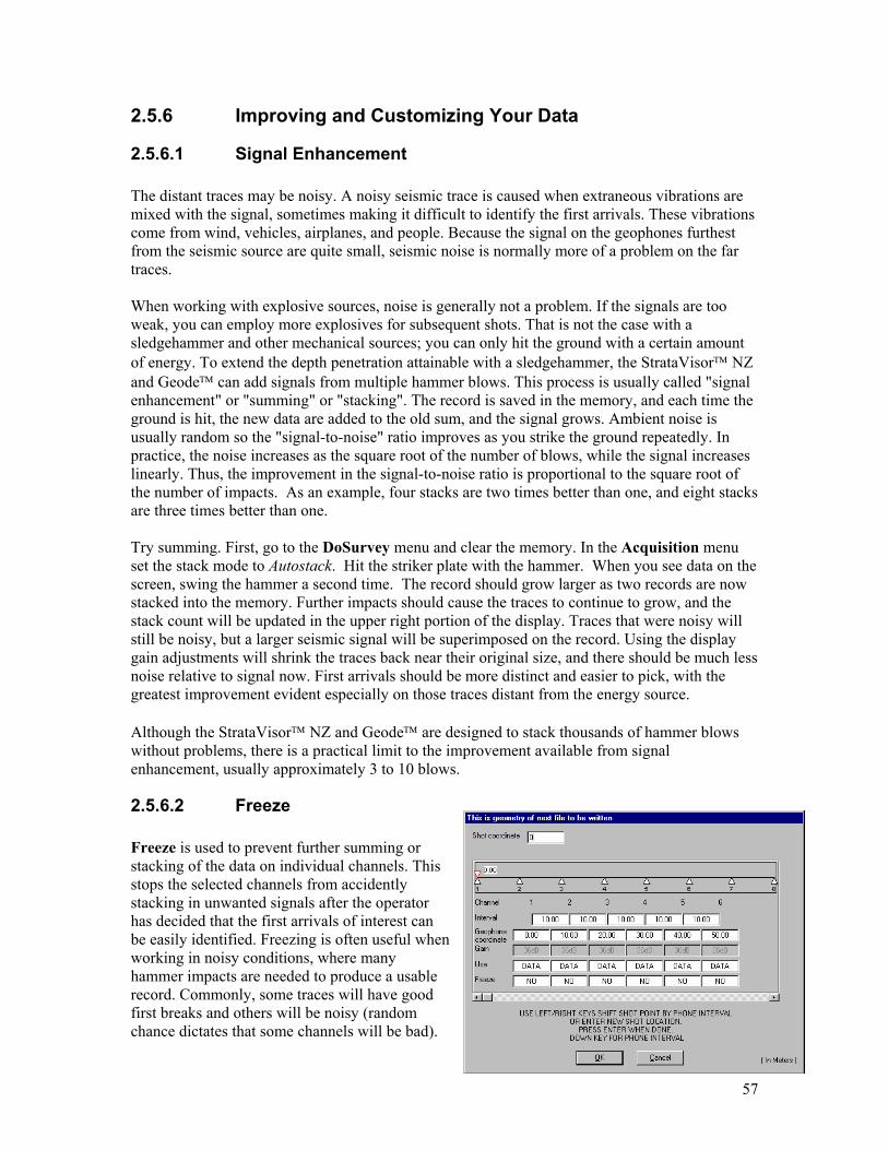
57
2.5.6 Improving and Customizing Your Data
2.5.6.1 Signal Enhancement The distant traces may be noisy. A noisy seismic trace is caused when extraneous vibrations are mixed with the signal, sometimes making it difficult to identify the first arrivals. These vibrations come from wind, vehicles, airplanes, and people. Because the signal on the geophones furthest from the seismic source are quite small, seismic noise is normally more of a problem on the far traces. When working with explosive sources, noise is generally not a problem. If the signals are too weak, you can employ more explosives for subsequent shots. That is not the case with a sledgehammer and other mechanical sources; you can only hit the ground with a certain amount of energy. To extend the depth penetration attainable with a sledgehammer, the StrataVisor NZ and Geode can add signals from multiple hammer blows. This process is usually called "signal enhancement" or "summing" or "stacking". The record is saved in the memory, and each time the ground is hit, the new data are added to the old sum, and the signal grows. Ambient noise is usually random so the "signal-to-noise" ratio improves as you strike the ground repeatedly. In practice, the noise increases as the square root of the number of blows, while the signal increases linearly. Thus, the improvement in the signal-to-noise ratio is proportional to the square root of the number of impacts. As an example, four stacks are two times better than one, and eight stacks are three times better than one. Try summing. First, go to the DoSurvey menu and clear the memory. In the Acquisition menu set the stack mode to Autostack. Hit the striker plate with the hammer. When you see data on the screen, swing the hammer a second time. The record should grow larger as two records are now stacked into the memory. Further impacts should cause the traces to continue to grow, and the stack count will be updated in the upper right portion of the display. Traces that were noisy will still be noisy, but a larger seismic signal will be superimposed on the record. Using the display gain adjustments will shrink the traces back near their original size, and there should be much less noise relative to signal now. First arrivals should be more distinct and easier to pick, with the greatest improvement evident especially on those traces distant from the energy source. Although the StrataVisor NZ and Geode are designed to stack thousands of hammer blows without problems, there is a practical limit to the improvement available from signal enhancement, usually approximately 3 to 10 blows.
2.5.6.2 Freeze Freeze is used to prevent further summing or stacking of the data on individual channels. This stops the selected channels from accidently stacking in unwanted signals after the operator has decided that the first arrivals of interest can be easily identified. Freezing is often useful when working in noisy conditions, where many hammer impacts are needed to produce a usable record. Commonly, some traces will have good first breaks and others will be noisy (random chance dictates that some channels will be bad).

58
Use Freeze to preserve the good traces, then focus on the noisy weak channels individually or in small groups. The advantage to freezing the channels with good signals is that they are protected from degradation during subsequent stacks. Freeze is also used in specialized surveys, such as when recording "Optimum Window" reflections (where you collect data on only one channel at a time) and borehole shear wave studies (where you might activate two channels while hitting one end of a plank, then two others while you hit the other end, then two others while you hit the top). To try this function, select Freeze from the Do Survey menu on the main menu bar (alternatively, you can get to the same place by choosing Group/Shot Locations in the Geometry menu). The bottom row of entry fields will indicate which channels, if any, are currently frozen. Position the cursor in the entry field of the channel you would like to freeze and press "2". It should change from “No” to “Yes”. Press ENTER. The channel numbers on the frozen traces will be displayed in reverse video. Clear the memory. Notice that the frozen channels remained on the screen. Hit the ground a few times and observe that the frozen channels do not change while the unfrozen channels will, growing with each impact. Unfreeze all the channels and clear the memory with the Clear Memory function.

59
2.5.6.3 Other Display Modes The visual attributes of traces can be changed in many ways to optimize the seismic events of interest. The different display style options are selectable in the Trace Style submenu under Display/Shot Parameters. The most common display setting is ‘wiggle trace’ to represent the motion of the ground at a geophone (shown opposite). Wiggle trace is a good mode for getting an overview of the record, but less useful than the other modes for most purposes. Once seismographs made the transition from analog to digital instruments, data were processed on computers. Interpreters found that if you shaded the positive trace excursions black, it was easier to see reflections in the record. The StrataVisor NZ and Geode offer this option, called "variable area". An example is shown in the figure below. Variable area is generally better for reflection surveys, although no reflections are visible in this record yet.
Variable area turns much of the record solid black, obscuring portions of the individual traces. This suggests another option, which has been called "shaded area". In shaded area, the positive excursions are shaded gray instead of black, and you can see individual traces even when they pass through the shaded portion.(shown opposite). Choose variable area or shaded area for reflection surveys, depending on which works best for an individual recording.

60
In refraction surveys, the first arrival of the wave at the geophone is the major event. In either variable area or wiggle trace, adjacent traces can swing over and obscure the first arrivals, especially when the display gain is increased to sharpen the first breaks. Clipped display format is a useful tool when adjacent events obscure first arrivals. However, a cautionary note about using clipped display format is in order. Although "clipped" is a better form for picking refraction records, it can obscure some characteristics of the waveform. Although it was suggested in the exercise above, to really see the seismic picture, you need the whole waveform, with background noise, first arrivals, sound waves, and surface waves displayed. Seeing the whole picture allows you to predict the location of the desired first arrivals almost exactly, and you should work with normal wiggle trace first, adjusting the display gain for the best image. Then, you can switch to the clipped format to eliminate overlap between traces. It will be very helpful to have the data stored on the hard disk or on the floppy disk, even though you may have a "pickable" paper record in the field. Experiment with these options. Hit the ground with the hammer to produce a new record on the screen. Change the display by switching the Trace Style to each of the other combinations. Observe the effect on the trace display. Print a copy if desired.
2.5.6.3.1 AGC Traces shown in this chapter have until now been displayed in "fixed" gain mode, which means that the display gain scale factor on a particular trace is constant throughout the length of the record (though the scale factor on individual traces may be different). Notice that each trace contains a quiet early portion, a large signal as the vibrations pass the geophone, and then often a quiet portion near the end where the signals weaken. For applications other than refraction (particularly reflection surveys) you might wish to use a different gain at different times in the record. The automatic gain control (AGC) performs this function, increasing or decreasing the display gain to keep the excursions at some reasonable value throughout the record. The StrataVisor NZ and Geode employ "digital AGC". The average signal in a user defined section of the trace, called a "window", is used to adjust the display gain (larger or smaller) for the data sample in the middle of the window time period. Then, the window is advanced slightly and the adjustment repeated for the next data sample. Digital AGC is able to look ahead in time, see a large signal coming, turn the display gain down in advance, and properly display large first arrivals. The record opposite shows a record with AGC applied; the very early portion of the record looks noisy on the far traces. This is normal, since the AGC increases the display
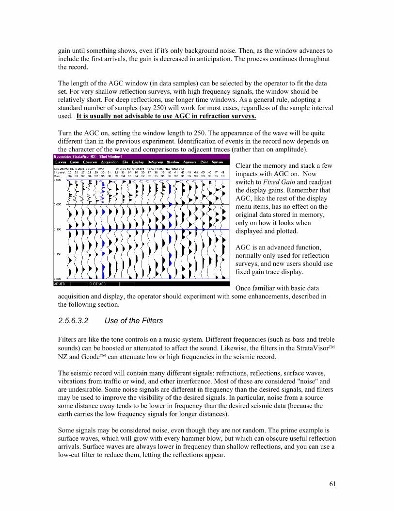
61
gain until something shows, even if it's only background noise. Then, as the window advances to include the first arrivals, the gain is decreased in anticipation. The process continues throughout the record. The length of the AGC window (in data samples) can be selected by the operator to fit the data set. For very shallow reflection surveys, with high frequency signals, the window should be relatively short. For deep reflections, use longer time windows. As a general rule, adopting a standard number of samples (say 250) will work for most cases, regardless of the sample interval used. It is usually not advisable to use AGC in refraction surveys. Turn the AGC on, setting the window length to 250. The appearance of the wave will be quite different than in the previous experiment. Identification of events in the record now depends on the character of the wave and comparisons to adjacent traces (rather than on amplitude).
Clear the memory and stack a few impacts with AGC on. Now switch to Fixed Gain and readjust the display gains. Remember that AGC, like the rest of the display menu items, has no effect on the original data stored in memory, only on how it looks when displayed and plotted. AGC is an advanced function, normally only used for reflection surveys, and new users should use fixed gain trace display. Once familiar with basic data
acquisition and display, the operator should experiment with some enhancements, described in the following section.
2.5.6.3.2 Use of the Filters Filters are like the tone controls on a music system. Different frequencies (such as bass and treble sounds) can be boosted or attenuated to affect the sound. Likewise, the filters in the StrataVisor NZ and Geode can attenuate low or high frequencies in the seismic record. The seismic record will contain many different signals: refractions, reflections, surface waves, vibrations from traffic or wind, and other interference. Most of these are considered "noise" and are undesirable. Some noise signals are different in frequency than the desired signals, and filters may be used to improve the visibility of the desired signals. In particular, noise from a source some distance away tends to be lower in frequency than the desired seismic data (because the earth carries the low frequency signals for longer distances). Some signals may be considered noise, even though they are not random. The prime example is surface waves, which will grow with every hammer blow, but which can obscure useful reflection arrivals. Surface waves are always lower in frequency than shallow reflections, and you can use a low-cut filter to reduce them, letting the reflections appear.

62
Another example of non-random noise is 60 Hz (50 Hz in many countries) electrical interference, often encountered when working in urban areas near power lines. “Notch” filters are provided to deal with this type of unwanted noise. Noise from wind may be either high frequencies (from wind blowing on the geophones) or low frequencies (from wind blowing on trees or buildings, which then push on the ground). Different types of filters can be used to reduce either type of noise. The StrataVisor and Geode systems offer two sets of filters: Acquisition and Display. The acquisition filters are "real-time" digital filters which operate on the incoming data just like traditional analog filters. When data is acquired with acquisition filters, their effect becomes part of the record stored in memory. The display filters, on the other hand, do not affect the numerical value of the data in any way. Display filters operate on the data after it is stored in memory. The type and corner frequencies can be changed to examine the effect of different filters on the stored data. When display filters are used, the filtered data is displayed on the screen and a paper copy can be plotted, but the original data is held in memory. If the record is saved on a disk, the original, raw data is saved, not the filtered result. This allows the user to select a different set of filters when the data is processed or read back into the seismograph for analysis. With the exception of notch filters, it is generally better to use display rather than acquisition filters to preserve the option for later changes during analysis. Low-cut filters are used to remove low-frequency signals (like surface waves, and noise from distant traffic). Notch filters are used to reject interference from power lines. High-cut filters attenuate higher frequencies, such as wind noise or nearby machinery. Each filter has a cutoff or "corner" frequency, which can be selected in the menu. Low-cut filters attenuate frequencies below the corner frequency, and high-cut filters attenuate frequencies above the corner frequency. Notch filters attenuate frequencies near their frequency, passing those above or below. Display filters are available in both 24dB/octave and 48dB/octave attenuation rates. To experiment with the display filters, select Display Filters in the Shot Parameters menu and select LOWCUT 15 HZ. You may need to first check the Enable Display Filters checkbox. Optimize the trace display and print a copy. Repeat the experiment with other, higher frequency, low-cut filter settings. Compare the records from each filter (including the one made earlier with no filter) to see the effect of the low-cut filter. If there is noise from a low frequency source, it should get progressively smaller as higher frequency filters are used. The first arrivals should grow more distinct, and then later fade away again as you pass into the frequency range where they are also filtered out. Note that selecting filters with a corner frequency close to the dominant frequency of the events you are viewing may shift the event in time. For this reason, when doing refraction surveying, limited filtering is recommended. There may be a range of filter settings where reflections are visible on the record. The low frequency surface waves should disappear when higher frequency low-cut filters are used. The figure below shows a record displayed in variable area with a 24 dB/octave low-cut filter (and AGC). This is the same survey line used for the previous examples; note that some of the low-frequency surface waves have been removed and a possible reflection is visible in the data between 90 and 100 milliseconds on the far traces.

63
Try the same experiment with the notch filters. These will be less dramatic in their effect on the record and changes may not be visible at all unless there is some power line noise present. Remember that ideally they will not change the character of the seismic record (although there is always some change in the signal from removing 50 or 60 Hz information). Since 3-phase power lines also radiate at three times the fundamental frequency, 150 and 180 Hz notch filters are also provided. Repeating the experiment with the high-cut filters should show some reduction in high frequencies, particularly at 250 Hz. This may be evidenced by rounding of first breaks or other effects. You will need to choose between acquisition and display filters. Acquisition filters have the disadvantage of permanence, but the advantage of eliminating so-called edge effects at the beginning and end of the record. In general, when a notch filter is required, it is better to select one in the acquisition menu.
2.5.6.4 Using Delay Normally, the seismograph begins recording data instantly when the source triggers. The Delay function is provided to postpone the start of the record by a selected time. This is applicable to surveys where there is a substantial distance between the shotpoint and the nearest geophone, and where there is no usable information in the early part of the record. Examples might be velocity logging of deep boreholes, or off-end shots in deep refraction surveys. To test the delay, take a sample record as was done earlier. Save the data using the SAVE function in the Do Survey menu. Then, in the Acquisition Timing menu, enter a delay of 10 to 20 ms. Repeat the shot with the delay and compare the two records. Notice that the record made with the delay has not recorded the early portion of the record, but has appended some additional time to the record. The time lines (and annotated time lines on the plotted record) are automatically adjusted for the delay values, so times picked on the record are referenced to shot time. Delay can also be set to a negative number, which means that the record will display some data prior to the actual trigger. This is helpful when using an energy source which is difficult to time

64
precisely, such as a weight drop or air gun. One of the seismic channels can be connected to the trigger signal or to a motion sensor near the source to record the time of impact, or "zero" time. Routinely using a little negative delay (~10 msec) will help the automatic first break picking program do a better job. Set the delay back to –10 msec.
2.5.6.5 Reducing the Number of Acquisition Channels The number of channels in use may be reduced when not needed. In borehole surveys, it is common to use only three geophones (or even one). Reducing the number of channels limits the size of the shot records, so that more records may be stored on a single disk. To change the number of active channels, clear the data and select Specify Channels in the Acquisition menu. Move the cursor to the channel you wish to disable and press “4” to make it inactive. This channel and all of those to the right of it will no longer be visible on the display and will not record data until reactivated. The channels are not renumbered when some of the channels are turned off.

65
2.5.7 Storing Data If you have used a seismograph before, you may have used an older device that produced a paper plot which you took home, picked the arrivals, analyzed, and interpreted. If that is the case, you know that records which looked fine in the field can suddenly develop poor first arrivals when examined in the office. Perhaps even the location was uncertain. The StrataVisor NZ and Geode will save the digital records on a disk. Once saved, they can be read back into memory, or read, displayed, and interpreted on a personal computer. This can be extremely useful, even for ordinary refraction surveys, since the records plotted in the field are rarely optimum and often difficult to pick. Plotting the records again in the office, and picking them from the screen or an optimized paper plot is a great improvement. Automatic refraction analysis on the computer is an even greater benefit. Digital recording and processing are required for reflection surveys. When recording data, it is generally advisable to save the data to the internal hard disk or an external tape driveMGOS (if you have a tape installed). To allow storage of your data, you must enable either Save to Disk and/or Save to Tape in the File/Storage Parameters. If saving to disk, indicate a path or folder. This is the folder your data will be stored in. See Chapter 4 (File Storage and Handling) for a discussion of tape drives and other storage media. Data may be transferred from the hard disk to 3.5" floppy via the internal floppy drive. Currently you must use standard WindowsTM file copying and transfer procedures. At this point, you should know how to acquire data, save it on disk, and read the data back. You should also be quite familiar with the use of the system menus. 2.5.8 Answers The Answers menu is used to analyze the seismic data. Programs are provided to allow a fairly complete seismic refraction solution, including layer depths and velocities which may be interpreted into geologic structure. A proper seismic refraction interpretation requires at least two records, each record acquired with the source at opposite ends of the line. More detail, and deeper information, can be obtained by also locating the source well off either end of the line and in the interior. For each shot, the Pick Breaks function will assist in picking the first breaks and saving the data on disk. Be sure that the line geometry is properly entered for each shotpoint. To help you remember, the StrataVisor NZ and Geodewill prompt you for geometry data at appropriate intervals if you are in the refraction mode. Geometrics recommends taking 5 to 7 shots per geophone spread to reduce possibilities for error and to best characterize the subsurface. However, this may not be necessary for surveys for characterizing larger features, like the weathering layer for petroleum surveys or ripability surveys to determine rock velocities.
2.5.8.1 SIPQC SIPQC is an interactive refraction interpretation program. It was originally developed by Jim Scott at the United States Geological Survey and has been commercialized under his company RimRock Geophysics. The software is now embedded in the StrataVisor NZ and Geode SGOS and MGOS operating software.

66
SIPQC uses first break pick files to generate a velocity cross section of the area under your seismic survey. It will calculate a depth at each geophone if the data is of sufficient quality and density, otherwise it will estimate depth under each shot point. Up to 7 shots can be used in the analysis. In the following exercise, we will use the data included on the data disks sent with your system. Take a minute to install the data as described in Appendix C. First, all of the data files must have their first arrivals picked. If you have not already done this with the sample data, take a moment to do this.

67
2.5.8.1.1 Selecting First Break Pick Files Next, select Answers from the DoSurvey menu and choose Solve Refraction Using SIPQC.
Choose the menu that contains the sample refraction data and choose 5 of the data files. You will be asked to give your spread a name that will help you track your interpretation.
The adjacent Time-Distance graph shows all of the first break picks from each of your shot records. Each pick has been replaced with a number indicating the layer that the seismograph program estimates the energy has penetrated to. Picks from the same shot point are joined by a straight line.

68
2.5.8.1.2 Layer Assignments The seismic program is not perfect at assigning layering and will often require editing to ensure that the interpretation program will operate properly. However, this can be accomplished by following a few simple rules. The point at which a series of picks changes from one layer to another is known as a hinge point (arrow, shown opposite). Hinge points are generally identified when there is a reduction in the slope of the line of picks. However, changes in slope can also be caused by irregular refractor topography. To check that this is not the case, you must compare the line of picks at the same location with another shot from the same side of the spread, but arriving later in time.
The figure opposite shows such a comparison. The lower shot (outlined in light grey) shows a potential hinge point at the 4th geophone. The shot above (outlined in dark grey) shows NO equivalent hinge point. This means that the hinge point on the first red t-d plot is valid and the numbers should progress from layer 1 to
layer 2.
Proceed by assigning layers to the t-d plot for each shot. This may take some practice and you should consult other books on refraction surveying to review the layer assignment process. Below, a figure is shown with all layers assigned for a two layer interpretation.

69
2.5.8.1.3 Running the Interpretation Once you are satisfied with the layer assignment, you can run the interpretation by pressing Continue. Depending on the speed of your computer, this may take a few seconds. A display similar to the one opposite will appear, showing a boundary between the assigned layers. Any suspect first break picks will show as question marks on the plot. Refer to the SIPQC manual for additional explanation of the emergent ray points.
To see a color version of the display with the calculated velocities, press Toggle Plot. The following display will be shown. You can return to the layer
assignment plot by pressing Back to try other layer assignments reflecting other interpretations. There may be other interpretation tools under the answers menu. Currently, we are offering for trial a version of Optim’s refraction interpretation package that requires no layer assignment and is more automated than the interpretation package discussed above. Please refer to the Optim documentation for more details.

70
2.6 Summary By now, you should appreciate that the StrataVisor™ NZ and Geode™ are extremely powerful and easy-to-use seismographs. Only a portion of the features have been discussed, and you should continue your familiarization by reading the rest of this manual and conducting further field experiments As a general rule, the seismograph is very forgiving, and will gather the highest quality data possible with a minimum of effort in the field. While we have concentrated on refraction, the StrataVisor™ NZ and Geode™ were designed for shallow and deep reflection, and are capable of both shallow and deep reflection, cross-well tomography, surface wave and VSP surveys. Geometrics can offer advice, short courses, and application notes to assist you. Don’t forget that many of the functions discussed in Chapters 1 and 2 are accessible as HOT KEYS, which reduces the number of key strokes and speeds operations. See a listing of the HOT KEYS under the DO_SURVEY menu.

71
3 Software and Interactive Menus
3.1 Introduction This section describes the software used to operate the ES-3000, the Geode and StrataVisor NZ and NZC. It includes detailed descriptions of the display, keypad, and interactive menus. The menu section is organized in a glossary style so that individual sections may be used alone to explain menu items in detail. There are four configurations available for data acquisition: ESOS (ES-3000 only), Single Geode Operating Software (SGOS), Multiple Geode Operating Software (MGOS) and Marine Multiple Geode Operating Software (MMGOS) useful for marine, tomography and VSP surveys where high cycle times are important. ESOS/SGOS software runs on laptop computers and has functions necessary for the collection, processing and interpretation of engineering-style geophysical surveys. SGOS can control from 3 to 24 channels in a single box.
ESOS on Laptop with ES-
3000
SGOS on Laptop with Geode
MGOS on Laptop with Geodes
NZ/C (comes standard with MGOS)
Comments
No. of Channels Per Line
8 and 12 3 to 24
3 to > 500 3 to > 240
Number of channels limited only by practical data size
No. of Geodes 1 1 Many Many
No. of Lines 1 1 Typically 2 Up to 4 MGOS operates up to 16 lines on desktop computer
Sample Intervals 64µs to 2ms 20µs to 16ms 20µs to 16ms 20µs to 16ms
Record Length 4K 16K 16-64K 16-64K
Geophone Testing No No Yes Yes
Analog Testing Not available Not available Available as built in or external
Available as built in or external
Future
Data Formats SEG2 SEG2 SEG2/Y/D SEG2/Y/D
OS Win98/NT/2K/XP Win98/NT/2K/XP Win98/NT/2K/XP Win98/NT/2K/XP 95 version available on web site
Data Storage Locally on OS structured media
Locally on OS structured media
Writes to DAT, DLT, 3480, 3490 etc
Writes to DAT, DLT, 3480, 3490 etc
Hardware Correlator No Yes Yes
Bandwidth See sample rates
1.7 Hz to 20 kHz 1.7 Hz to 20 kHz. Lower corner available
1.7 Hz to 20 kHz. Lower corner available
Repeater No No Yes Yes
Preamp Gain 24 and 36 dB software
selectable
24 and 36 dB software
selectable
12/24 dB or 24/36 dB or 0 dB
12/24 db or 24/36 db or 0 db
gains are software selectable, gain pairs are jumper
selectable Roll Capability No No Yes Yes
Real-Time Spectral Display
No No Yes Yes

72
MGOS software runs either on a laptop computer, or comes standard on the StrataVisor NZ/C seismograph. It contains all of the functions found in SGOS, as well as all of the additional data management protocol required for larger scale surveys with large numbers of channels or large numbers of Geode modules. The following table summarizes the differences between the two software packages. This manual describes all configurations of software simultaneously, as ESOS and SGOS are subsets of MGOS. Marine MGOS (MMGOS) has additional features. Sections of the manual that describe features that are exclusive to MGOS will be shown with MGOS as a superscript in the section heading, shown as follows:
2.x.x This is a section describing an MGOS feature MGOS
Features that are specific to Marine MGOS have the superscript MARINE . In addition, there are several additional options that can be purchased separately. These features are designated in the manual with an OPTIONAL superscript. This list of options is ever- expanding, so please contact the factory or check our web site for the latest updates.
3.2 Installing the software on your system Please refer to Appendix B.
3.3 Running SGOS or MGOS Software for the First Time Please refer to Section 2.

73
3.4 Accessing the Menu Structure Using the Front Panel Keypad on the StrataVisor NZ.
3.4.1 Color Screen The keypad on the NZ system has 21 keys, including numbers 0 through 9, MENU, ENTER (shown as a return arrow ↵), Func, CLR (clear), "-" (hyphen or minus), "." (decimal point), “TAB”, and 4 arrow keys. Every effort has been made to render the operating software fully operational from the keypad, precluding the need for a mouse. Still, as the WindowsTM operating system was designed around the mouse, you might find it useful to have one handy for special operations such as customizing your display, as well as operations outside the StrataVisorTM
acquisition software. It is assumed that the reader is reasonably versed in operating WindowsTM -based programs. 3.4.2 Functions of the Keys The MENU key is used to select the operating menu. Pressing this key automatically takes you to the DoSurvey menu, since this is the menu most often used while surveying. The arrow keys are used to position the cursor among menu options on the screen. The left arrow key can also be used as a backspace to delete the last digit when entering a string of numbers. CLR is used to back out of the menu or to recover from errors. ENTER or "↵" is used to confirm a selection after positioning the cursor or after keying in a number. "−" is used to designate a negative number or to designate a range of numbers, i.e. 1-12 (for numbers 1 through 12). "." (decimal point or period) is used to insert a decimal point or to act as a left mouse click to fill in check boxes. The TAB key moves control from entry field to entry field. It works slightly differently than the arrow keys. The best way to understand the functions of these and the rest of the keys is to practice. You will become fluent with their operation in a short time. The Func key enables access to the menu quick keys that precede each menu item on the main menu. For example, pressing Func then 2 accesses the Geometry menu.
3.4.2.1 Hot Keys Hot keys provide single keystroke access to many of the important functions in the SGOS and MGOS menu structure. They are an easy and powerful way to navigate complicated software. There are two kinds of hot keys in the M/SGOS operating systems

74
• Global, which work no matter what window is open or active • Local, which pertain to a particular window being ‘selected’.
3.4.2.1.1 Global Hot Keys The following table lists all global hot keys. Note that some keys are slightly different on the StrataVisor NZ seismograph since its weatherproof keyboard is more limited.
Function Geode NZ
Arm/disarm 1 1 Clear data with warning
dialog box to clear data with default button set to yes
2 2
Activate geometry Dialog Box
3 3
Maximize noise monitor window
4 4
Maximize shot record window
5 5
Autoscale traces 6 6 Save data 7 7
Print shot record 8 8 Correlate 9 9
Restore windows 0 0 Toggle active window TAB TAB
Roll right Ctrl-End FUNC → Roll left Ctrl-Home FUNC ←
Manual trigger t
Most global hot keys activate menu items in the DO_SURVEY menu. The DO_SURVEY menu is shown opposite which controls the majority of the operation of a seismograph once it is set up. The seismograph can be ARMED or DIARMED using the 1 and 0 keys from the keypad or keyboard. You can quickly maximize the noise window with hot key 4, autoscale traces with hot key 6 or print a record with hot key 8.

75
3.4.2.1.2 Local Hot Keys – Shot Window Selected When the shot window is selected, the following keys are active. Particularly handy are the increase/decrease trace size option and the increase/decrease time scale.
3.4.2.1.3 Local Hot Keys - Noise Window Active
Function Geode/ ES-3000 NZ Increase/decrease pilot
sensitivity → ←
→ ←
Increase/decrease sensitivity
↑↓ ↑↓
3.4.2.1.4 Local Hot Keys - Pick Window Active
Function Geode/ ES-3000 NZ Print picked traces 8 8
3.4.2.1.5 Local Hot Keys – Log Window Active Function Geode/ ES-3000 NZ
Scroll up or down ↑↓ ↑↓ Page up or down PAGE Up/Down FCN ↑↓
3.4.3 External Keyboard and Laptop Keyboard Your seismograph may also be operated from an external computer-style keyboard with a PS-2 connector. Just plug the keyboard into the connector provided (some keyboards may require being plugged in during boot-up). With an alphanumeric keyboard, folders, project names, and other
Function Geode NZ Scroll ↑↓ ↑↓
Increase/decrease time scale
PAGE Up/Down FCN ↑↓
Increase/decrease trace size (all) when in fix gain
Otherwise gain style
→ →
Increase/decrease trace size (individual) when in fix gain
Otherwise gain style
← ←
Toggle trace clipping “-“ “-“

76
parameters may be named with letters as well as numbers. However, it is recommended that shot record file names be numerical, as this is what most processing software will be expecting.
3.4.3.1 Using Keyboard Short Cuts to Get Around Menus Some form of pointing device is the preferred way of operating a Windows based operating system. However, this is often not practical in the field as there are seldom flat surfaces to steady the hand. Instead, you may find it more appropriate to navigate to items in the menus using the ALT key on the keyboard and the letter or number associated with each menu. The key to be pressed in conjunction with the ALT key is always underlined and is either IN the name of the menu, or in front of the menu selection. For example, you can quickly get to the Display Boundary options in the display window by pressing ALT 6, followed by 1 then 1 again.
Attempting this sequence in the field with a mouse or with a touch pad can be frustrating without a steady surface. Keyboard short cuts are much quicker.

77
3.5 Detailed Description of Menus There are four separate windows that can be displayed at any given time for MGOS software. The spectral window is absent in SGOS software. Like any WindowsTM -based program, these windows can be positioned and sized at will, and your settings will be remembered from session to session. If you have an NZ based portable system, you will need to plug in a mouse to accomplish this, but once it is done you should not need a mouse in the field. The system is designed to be fully operational with the built-in keypad. On initial power-up of your software, you should see the following:
You may or may not see the Geometry GUI, a window which gives you a graphical representation of the ES-3000/Geodes on the line. The Geometry GUI is described separately in section 3.8.

78
Users of SGOS software will see windows: the shot, the noise display, the log file and the geometry GUI. The spectral window will be missing.
Across the top you will see the list of main operational menus. Within each are a selection of submenus. Before we get in to the description of these, we will first discuss each of the four main display windows.
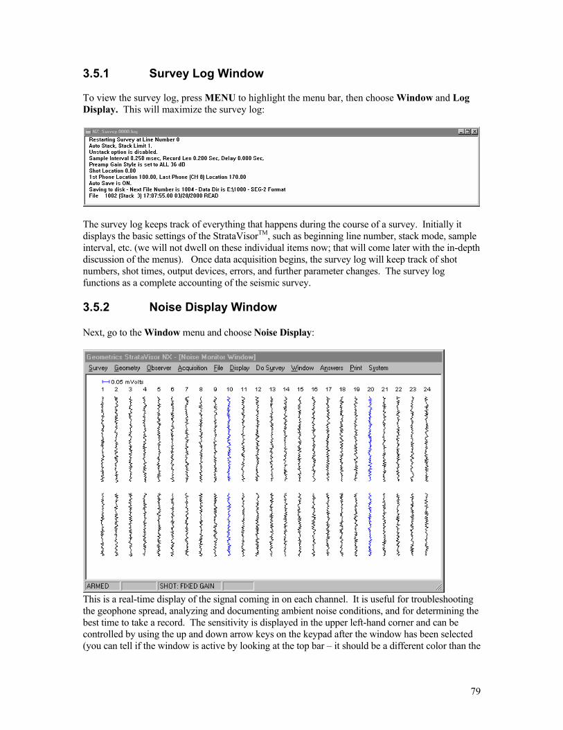
79
3.5.1 Survey Log Window To view the survey log, press MENU to highlight the menu bar, then choose Window and Log Display. This will maximize the survey log:
The survey log keeps track of everything that happens during the course of a survey. Initially it displays the basic settings of the StrataVisorTM, such as beginning line number, stack mode, sample interval, etc. (we will not dwell on these individual items now; that will come later with the in-depth discussion of the menus). Once data acquisition begins, the survey log will keep track of shot numbers, shot times, output devices, errors, and further parameter changes. The survey log functions as a complete accounting of the seismic survey. 3.5.2 Noise Display Window Next, go to the Window menu and choose Noise Display:
This is a real-time display of the signal coming in on each channel. It is useful for troubleshooting the geophone spread, analyzing and documenting ambient noise conditions, and for determining the best time to take a record. The sensitivity is displayed in the upper left-hand corner and can be controlled by using the up and down arrow keys on the keypad after the window has been selected (you can tell if the window is active by looking at the top bar – it should be a different color than the
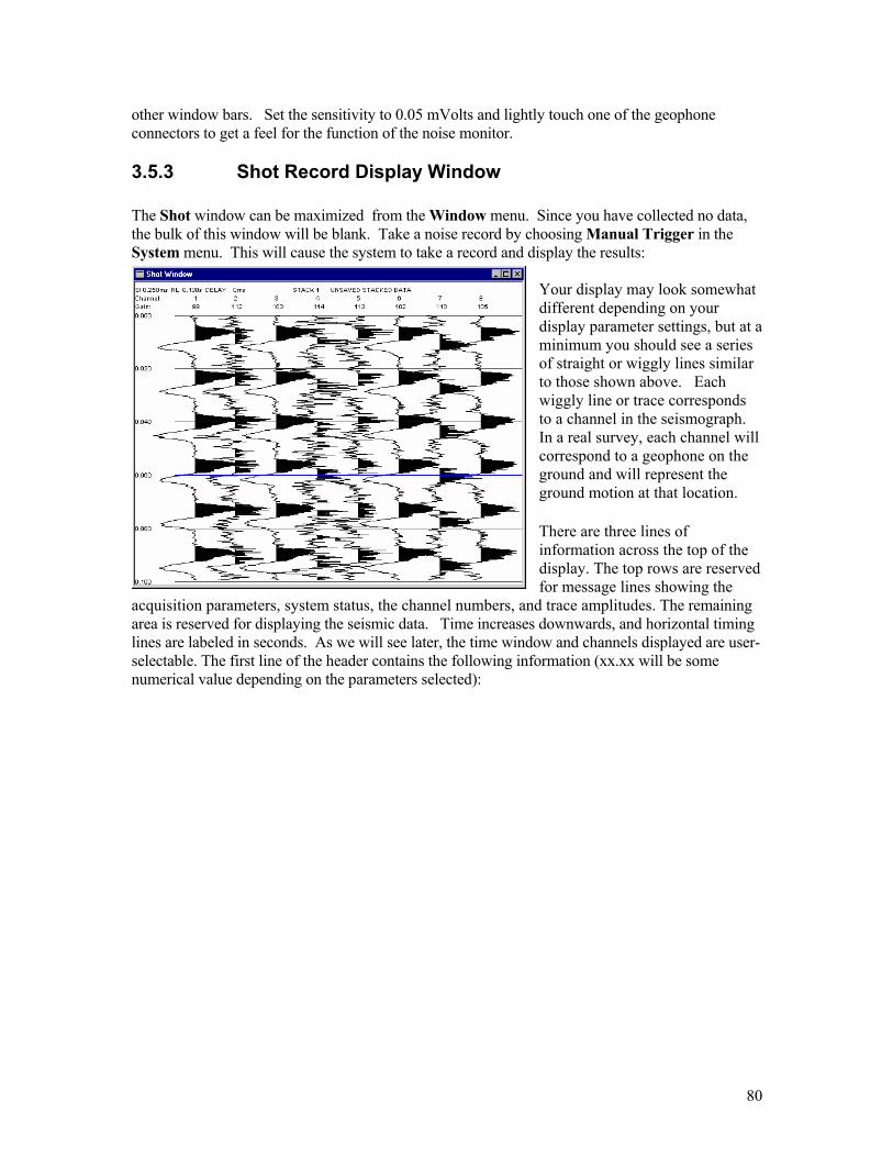
80
other window bars. Set the sensitivity to 0.05 mVolts and lightly touch one of the geophone connectors to get a feel for the function of the noise monitor. 3.5.3 Shot Record Display Window The Shot window can be maximized from the Window menu. Since you have collected no data, the bulk of this window will be blank. Take a noise record by choosing Manual Trigger in the System menu. This will cause the system to take a record and display the results:
Your display may look somewhat different depending on your display parameter settings, but at a minimum you should see a series of straight or wiggly lines similar to those shown above. Each wiggly line or trace corresponds to a channel in the seismograph. In a real survey, each channel will correspond to a geophone on the ground and will represent the ground motion at that location. There are three lines of information across the top of the display. The top rows are reserved for message lines showing the
acquisition parameters, system status, the channel numbers, and trace amplitudes. The remaining area is reserved for displaying the seismic data. Time increases downwards, and horizontal timing lines are labeled in seconds. As we will see later, the time window and channels displayed are user-selectable. The first line of the header contains the following information (xx.xx will be some numerical value depending on the parameters selected):

81
SI xxxx is the sample interval in milliseconds. RL xxxx is the record length seconds. The StrataVisor allows the use of all or part of the available memory, so the record duration will depend on the combination of sample rate and record length. DELAY xxxx is the delay in the start of the record (in milliseconds) after the trigger signal, or if negative, the amount of data prior to the trigger signal. AF indicates that acquisition filters are enabled. DF indicates that display filters are enabled. STACK xxxx indicates how many stacks are currently in memory. AGC or FIXED will indicate the gain style setting (no indication of gain style indicates that it is set to NORMAL).
A message indicating the status or type of data will be displayed in the upper right hand corner of the screen: MEMORY CLEAR indicates the memory has been cleared – no data, and the stack count should be zero. UNSAVED STACKED DATA is seismic data stacked into the memory (but not saved on disk). SAVED AS xxxx.DAT indicates the stacked data has been saved on disk (in file XXXX.DAT). READ FROM xxxx.DAT indicates data read from disk (from file xxxx.DAT). The remaining two lines in the display header show the channel numbers and the relative trace sizes or display gains. Relative trace amplitudes are labeled in dB. Amplitudes are accurately displayed, so that absolute amplitude comparisons can be made when the traces are displayed in fixed gain (as opposed to AGC, or automatic gain control). In systems with 48 or more channels, there may not be enough room to label every channel. In that case, we label as many as feasible. 3.5.4 Spectral Window MGOS The spectral window shown line spectra of each trace defined in the display window. Note that the spectral window is a MAJOR user of CPU time. This window should be closed when operations requiring the controller CPU are more critical.

82
3.5.5 Gather Windows MARINE The gather window is used in marine surveys to look at a single trace from each shot gather. The operator can select which trace should be plotted in the DISPLAY>Gather Parameters menu. Up to 3 gather windows can be displayed simultaneously.
3.5.6 Trigger Timing Window with Gun Energy Monitor MARINE The trigger timing window is used in a marine survey to watch for variations in the shot cycle time or missed shots, indicative of problems with the navigation system or a measure of system overloading. This is a combined bar graph display, with the upgoing (positive) bars showing the time between successive shots, and the downgoing (negative) showing the cumulative energy in a single trace. For the gun energy monitor, typically a hydrophone is placed near the gun, or sometimes the nearest hydrophone is used. Warning thresholds can be set for either the shot timing and gun energy histograms. When thresholds are exceeded, the traces turn a different color, as shown in the window below. Display parameters can be set in the DISPLAY>Trigger Parameters dialog box.

83
3.5.7 Noise Window MARINE The Noise Window bar graph provides a ‘snapshot’ of the noise at any user defined moment in the acquisition cycle, typically at the very beginning of the record or at the very end. A display threshold can be set, above which a noisy trace will turn red. The noise window bar graph is often a requirement on client-monitored surveys. Noise monitor display parameters can be changed in the DISPLAY>Noise Parameters dialog box.
3.5.8 Geometry Graphical User Interface The Geometry GUI provides a graphical representation of your survey, along with a wide range of control capability. It is particularly useful when conducting reflection surveys, but can be useful in a wide range of applications. It summarizes, in one simple view, the physical positions and other attributes of the hardware on the ground, and allows graphical control of these.
The Geometry GUI (GGUI) operations are extensive and are described in section 3.8.

84
3.6 Status Bars 3.6.1 Main Menu Bar The main menu bar has been organized to follow the convention suggested and approved by many of our users over the years. Owners of previous Geometrics instruments such as the StrataVisor R and RX, the SmartSeis and the ES-2401 will recognize the left to right convention for setup and operation. The main menu selections are displayed at the top of the screen:
When the MENU key is pressed on the StrataVisor NZ, the Do Survey menu will drop down and a secondary menu showing the corresponding choices appears. If you are using a laptop or computer, you can use your pointing device to highlight the menu items or use the ALT key in combination with any of the preceding numbers in the selections in the main menu. For example ALT- 7 pulls down the Do-Survey menu, similar to pushing the MENU key on the StrataVisor. The secondary menu items have numbers in front of them. You can select an item by pressing the corresponding number key instead of moving the cursor. Pressing the number key to select a menu item will be much faster when conducting actual surveys, especially after the operator has learned the numbers. In addition, some selections have "hot keys" that allow them to be selected without actually entering the menu. Any selection with a number to the right is hot-key enabled. For instance, you may arm the system from outside the menu system by simply pressing 1 (see the DoSurvey menu). Survey menus are used for setting up and naming a new survey. Geometry menus are used to record the locations of the geophones and the energy source. Observer menus are used to set up the survey log and update the line and shot record number. Acquisition menus control the data gathering parameters (such as sample interval, record length, filters). File menus control the saving/reading of data files to/from disk. Display menus control the way the data is displayed on the screen and plotted. DoSurvey contains the functions normally used to acquire, display, and analyze data in a production mode. Window menus are used to maximize and minimize individual display windows. Answers menus are used to run the field quality control software programs to analyze the data.

85
Print menus control printing related parameters. System menus are used for general operating and test functions. Experiment with the system. The complete menu structure is listed on the following pages. Many secondary menus have a status indication, which identifies the current setting. The current settings in the following examples are representative. The actual menus will display many other alternatives. 3.6.2 Bottom Status Bar Across the bottom of the SCS window, there is a status bar shown with important information regarding the mode that the software and hardware may currently be in.
The leftmost box displays the system status, an important part of the survey. Possible status messages include:
Status Description Armed Ready to acquire data Disarmed Data acquisition disabled Acquire Collecting data on A/D cards Busy Undertaking system management Sending data Transferring data from A/D cards to computer Receiving Pilot Getting pilot from pilot channel Sendintg Pilot Transferring pilot to A/D cards to use correlator Processing Data Undertaking correlation or other signal processing
The next box indicates whether sampling is underway on the A/D cards. The 3rd box indicates the display mode for the shot window. The 4th box displays the stack count. The 5th box displays the status of the data, which can include:
Memory Clear Unsaved Stacked Data
Saved as file xxx.dat (Stacked Data) Saved as file xxx.dat (Correlated Data)
The 6th box displays the current location of the shot.

86
3.7 Interactive Menus 3.7.1 Survey
3.7.1.1 New Survey
The Survey menu is used to provide a name for the survey, an initial line number, and if writing to tape, an initial tape label MGOS. It is recommended that numbers be used for the line number and tape labels. The Survey Name will be the file name for the survey log. This log is displayed in the Survey Log window, and will be saved in standard ASCII format. It may be printed off line with any text editor, such as Wordpad, and can be archived along with the seismic data. The Initial Line Number is useful if you intend to include numerous geophone spreads into one “survey”. In this case, you would update the line number (see the Observer menu) each time you picked up and moved the spread. If you intend to begin a new “survey” with each new geophone spread, the line number may or may not be useful, depending on how you choose to do your bookkeeping. If writing to tape, the Initial Tape NumberMGOS is a useful parameter in that the survey log will indicate the tape number that each file is written to. When the tape is full and the operator inserts a new tape, the tape label number will automatically increment. It is good practice to label each tape with the appropriate tape number. By referring to the survey log, locating specific shot records will be greatly simplified.

87
3.7.2 Geometry Geometry is a collection of menus used to annotate the seismic data with the locations of the geophones and seismic source. The SEG-2 standard provides space in the header for 3-dimensional coordinates (X, Y, and Z) for the energy source and each geophone group. The information in the Geometry menu is optional, and surveys may be conducted without reference to this menu. However, its use is highly recommended as this information is essential when using the Answers functions. Some third-party interpretation packages also use this information. This information will be attached to the data when the file is saved to disk. If a file is read from disk, the coordinates displayed in the following menus will be from the data read in. The information read from the disk file can be printed on the paper records. Proper use of these capabilities will label each file with the geophone geometry and source location.
3.7.2.1 Survey Mode
When you are in Refraction Mode, the seismic software treats some of the data scaling operations differently. Autoscaling operations are done based on the amplitude of the noise before the first breaks to minimize the amount of manual scaling that may be necessary Reflection Mode trace autoscaling is done by
normalizing each trace to the maximum value of the trace shown on the display. If Refraction Mode is selected, Gap will be grayed out).
3.7.2.2 Group Interval The Group Interval is the distance between geophones or groups of geophones. Units are set in the System menu. If you are working in stations (i.e., one station equals x feet or

88
meters), then the units you set are irrelevant. Be aware, however, that the functions in the Answers menu require units of feet or meters to accurately perform calculations of depth or velocity. If you intend to use these functions, you must base your coordinates in one of these two units.
3.7.2.3 Group/Shot Locations This dialog box allows you to assign physical locations of the geophones to the channel numbers and to the shot position. The title bar of the dialog box indicates whether the coordinates displayed refer to either
• The next file to be written • A file that was read in from a mass storage device
The geometry that you choose will also affect the coordinates displayed in the Geometry GUI, described in section 3.8.
3.7.2.3.1 Navigation in the Geometry Dialog Box Several keys are used for navigation within the five categories of information accessible in the menu – shot coordinate, geophone interval, geophone coordinate, use and freeze:
• The TAB key and up/down arrow keys are used to navigate from category to category. • When in the Shot Coordinate box, the left and right arrow keys are used to increment or decrement the shot coordinate by the default group interval. • In any other box, the left/right arrow keys are used to navigate to the next or preceding entry within a category.

89
Regardless of the number of channels, only the positions of six channels are displayed at a time. To view a different segment of the geophone spread, simply tab or use the arrow keys to move to the right (or if using a mouse, use the scroll bar). You will see the channel numbers change accordingly.
3.7.2.3.2 Entering new values in the geometry fields You can type a new coordinate into the Shot, Interval or Geophone Coordinate categories. A new value is ‘accepted’ in each of these categories by pressing the TAB, UP/DOWN arrow keys or ENTER key. Special care should be exercised when entering data in the Shot Coordinate box as accidentally pressing the RIGHT or LEFT arrow keys will increment or decrement the shot value, probably to an unwanted value. If you make a mistake typing an entry in any box, you can simply move to another category and return to the box that you wish to revise. The entire number will be highlighted, indicating that it will be replaced with the new value that you type in.
3.7.2.3.3 Shot Coordinate If you know the coordinate of your shot, you may enter it next to Shot Location. The shot point location can also be set by positioning the cursor over the shot point location field and using the left and right arrow keys. The shot will be moved in increments equal to the group interval. This is useful in that it doesn’t require the actual coordinate of the shot to be known, just its location with respect to the geophones. You may know you want the shot between geophones 5 and 6, but you may not know the actual coordinates of that position. Move the cursor as close to that position as possible, and then fine-tune it based on the positions shown for the relevant geophones.

90
3.7.2.3.4 Geophone (Group) Interval When you first define a survey, the interval between geophones (group) is set to whatever number was entered in the Interval dialog box discussed above. However, you now have the flexibility to edit individual group intervals – this need not be constant throughout the spread. These values will be retained until they are globally reset in the Interval dialog box.
3.7.2.3.5 Geophone Coordinates Physical coordinates for each seismograph channel are assigned in the Geophone Coordinate boxes. You will notice that that as you enter new geophone coordinates, the values before and after the coordinate that you enter will be recalculated using the geophone interval set in the line above. This ‘rippling’ effect allows rapid repositioning of the line based on the less variable group interval, rather than having to type a new location at every geophone location. If you are entering a complicated geometry that has missed locations and non-equal phone intervals, you will probably want to set the interval values first before assigning coordinates.
3.7.2.3.6 Channel Use Channels can be designated as DATA, AUX, PILOT or INACTIVE. Note that any assignment of a channel use ripples to the right only, to facilitate setting many channels the same. DATA channels are standard acquisition channels used for recording data. They have an associated coordinate and geophone interval. DATA and INACTIVE channels are used to define the limits of the active spread in preparation for rolling a subset of contiguous channels either forward or backwards through the total number of channels available in the system. When channels ‘roll’, they take on the attributes of an neighboring channel (either DATA OR INACTIVE). See the section on ROLLING under DO_SURVEY for more description). AUX channels are used for recording ancillary data during a survey. This may include shot timing, uphole data, vibrator information or any other time series. Regretably, AUX channels also currently have an associated position, which must be accounted for when you have AUX channels in the middle of the spread (see note below). AUX channels do not roll (see section on ROLLING CHANNELS). Once an AUX, always an AUX, and it is unaffected by the rolling process.
Note regarding AUX coordinates: Whenever possible, AUX channels should be connected at the end (preferable) or beginning of the geophone spread. This simplifies the assignment of geometry since AUX channels have an associated geometry. However, occasionally it is necessary for the AUX channels to be in the middle of the spread, particularly when using a two line Geode system with only two network cards in the controlling PC. To avoid the AUX channels occupying a coordinate location that should be used for a geophone, the interval between the AUX channel and the previous channel should be set to 0.0. There may be some situations in which it is useful to assign an AUX channel with a coordinate. A bad geophone could be marked as an AUX to distinguish it from its

91
neighbors so it can be identified by the processing software. If parts of a geophone spread cable are unused, they could be marked as AUX along with a 0 coordinate interval to distinguish them from their neighbors. These channels can also be FROZEN (see below) so they will not collect data, and are easier to identify by subsequent processing
The PILOT channel is used to record data from a vibratory source to be used in the correlation process. There can be only one pilot channel. The pilot channel does not roll. INACTIVE channels do not collect data. Inactive channels hold a coordinate position and a group interval, and can assume the attributes of adjacent channels when rolling. FREEZE function stops data collection on a channel. This feature is useful in refraction surveys once the first break is clearly identifiable on channels near to the shot, but additional stacks are required on far offsets. Similarly, FREEZE is useful to eliminate data altogether on channels that have bad geophones or bad data. The FREEZE function does not ROLL when the ROLL RIGHT or ROLL LEFT function is applied (See description under DO_SURVEY menu).
3.7.2.3.7 Setting up a simple active spread in preparation for ROLLING If you are undertaking a reflection survey, you may want to set a group of channels to ROLL through the total number of available channels. In the example opposite, channels 2 to 4 have been set as DATA channels and channels 1, 5 and 6 have been set as inactive channels. If the operator ROLLS
RIGHT , channel 2 will be made INACTIVE and channel 5 will be changed to a DATA channel. Remember that PILOT, AUX and FREEZE channels do not roll. The ROLL function is usually performed with the SHOT INCREMENT and CHANNEL AUTO ROLL functions set to permit hands-off operation.
3.7.2.4 Phone Increment
3.7.2.4.1 Phone Increment: Reflection Surveys Using Mechanical Roll Switch
The Phone Increment is typically used in CDP-style reflection surveys and updates the physical coordinates of the active geophone spread when using an external roll switch. A mechanical roll switch physically changes the connections between the geophones and the channels of the seismograph. The roll switch

92
allows a contiguous subset of active geophones to maintain a fixed distance to the shot as it moves over the area of the seismic survey. For instance, when conducting a common-depth-point (CDP) reflection survey, normal procedure is to lay out a spread of geophones, connected to the seismograph through the roll switch. The number of geophones on the ground is larger than the number of channels in the seismograph, and the roll box controls which geophones are active (i.e., connected to the seismograph) at any given time. After each shot, the source and active segment of the geophone spread are incremented forward or “moved up”. No geophones or cables are actually moved physically, but the geophones that are now connected to the seismograph are different than before. Example: when the first shot is recorded, ground stations 1 through 24 (out of a total of, say, 48) are connected to channels 1-24 on the [24-channel] seismograph. Then, the shot is moved up (generally by a distance equal to the group interval), and the active portion of the spread is also moved up using the roll switch. For the second shot, ground stations 2 through 25 are now connected to channels 1-24 on the seismograph. For the third shot, you are recording from ground stations 3 through 26, and so on. Setting the shot and geophone increment appropriately will allow the seismograph to keep track of shot and geophone coordinates automatically, precluding the need for the operator to update this data after each shot. This is very useful, particularly in production seismic surveying. In practice, any sequence will be interrupted eventually. In that case, just enter the correct values for the line geometry before saving the file. If the geometry changes (different group interval for example), just update the information.
3.7.2.4.2 Phone Increment: Reflection Surveys Using Built In Software Roll The Phone Increment is usually set to zero for reflection surveys that employ the MGOS internal roll function (see DO_SURVEY menu). The rolling process, which changes channels on the trailing edge to INACTIVE and changes channels at the leading edge the of the spread to DATA, facilitates incrementing of the geophone coordinates.
3.7.2.4.3 Phone Increment for Refraction Surveys For most refraction work, you should set the phone increment to zero.
3.7.2.5 Shot Increment Shot Increment is added to the current Shot Coordinate after data are saved. See above discussion on Geophone Increment. The shot increment is typically non-zero for surveys involving either an external roll switch or the internal software function.

93
Type of Survey Shot Increment Phone Increment Refraction Adjusted manually Usually 0 Downhole Typically zero Usually non-zero
Reflection (External Roll Box) Automatically incremented after each
save
Usually non-zero
Reflection (Internal Roll Function) Automatically incremented after each
save
Usually zero
For most refraction work, you should set the shot increment to zero.
3.7.2.6 Gap Not currently implemented in the software. To be completed at a later date.
3.7.2.7 Automatically Rolling Channels
When data are saved, you can elect to have the group of active channels automatically ROLLED forwards or backwards. In combination with the SHOT INCREMENT, this completely automates the ROLLING function so the operator may concentrate on the observer’s log and notes. To turn on automatic rolling, check either the Enable Auto Roll Up/Right on save radio button, or the Auto Roll Down/Left on save radio button. You can also enter the number of channels (geophones) that the system will roll in the Geophone Roll Increment field.

94
3.7.3 Observer The Observer menu allows you to enter basic information about the survey: who the client is, the job #, site name, etc. This is also where you update the line number if you start a new "line" within a survey.
3.7.3.1 Edit Survey Description Use the Edit Survey Description utility to input job-specific information. This is completely customizable, and there is no limit to the amount of information you may enter here. You will likely create your own company template, which will be automatically remembered from session to session. The information entered here will be located at the beginning of the survey log. Obviously, you need an external keyboard to take full advantage of this feature.
3.7.3.2 New Line Number Depending how you conduct your survey and do your bookkeeping, you may prefer to break your survey out in terms of "lines". For instance, you may open a survey, and that survey may consist of several parallel refraction lines. They may be end-to-end or side-by-side. How you define the terms

95
"survey" and "line" is entirely up to you. A survey may consist of one line or a group of lines. A line may consist of one or several end-to-end geophone spreads. In any case, changing the line number in the middle of the survey simply updates the Survey Log. The data itself is not effected. If you elect to change the line number, you will also be given the opportunity to update the file number if you wish. However, changing the line number does not affect your data storage parameters -- the data will still go to the same directory or folder. Consequently, if you update the file name within the same survey, you must take care to provide a unique file name. The StrataVisor will not allow existing files to be overwritten -- you will be warned in this eventuality.

96
3.7.4 Acquisition This set of menus contains the acquisition parameters, those variables which affect how the data is collected. If newly acquired data is in the memory, the system will not allow you to change most of these parameters until you erase the data from memory, because stacking records with different acquisition parameters is illogical. For example, there is no logic in changing the sample rate between stacks. Attempting to change these parameters without clearing memory will result in a prompt to either save the data first or clear the memory. Acquisition parameters are permanent in their effect on the data (unlike display parameters). You cannot change the sample interval, record length, or filters once the data is in memory or saved on disk.
3.7.4.1 Acquisition Timing
A seismic signal is continuous. When this continuous (or analog) signal enters the seismograph, it is digitized at even intervals and the resultant numbers are stored in memory. The Sample Interval is the time interval between data samples. The sample interval is selected to match the scale and type of the survey. Smaller sample intervals (faster sample rates) should be used for short surveys in hard materials (such as rock and concrete). Slower sample rates are used for long refraction surveys and reflection surveys where events of interest arrive late in time. Note: The ES-3000 hardware does not support all of the sample rates and record lengths displayed in this manual.
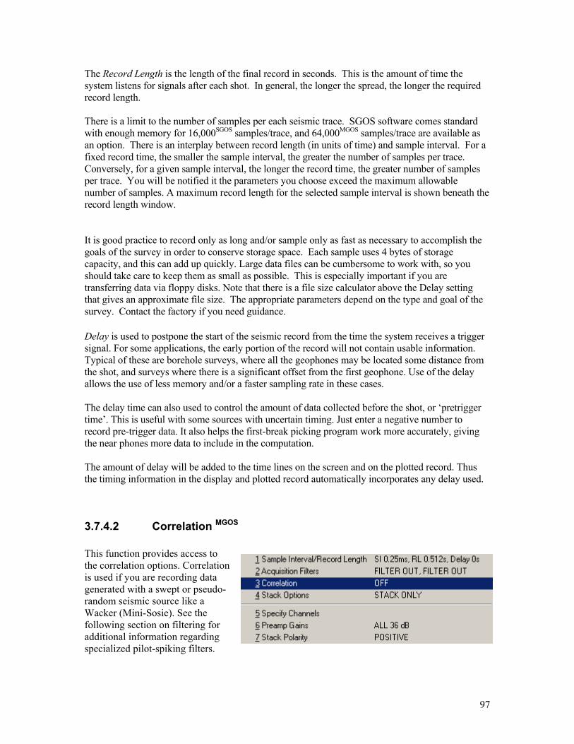
97
The Record Length is the length of the final record in seconds. This is the amount of time the system listens for signals after each shot. In general, the longer the spread, the longer the required record length. There is a limit to the number of samples per each seismic trace. SGOS software comes standard with enough memory for 16,000SGOS samples/trace, and 64,000MGOS samples/trace are available as an option. There is an interplay between record length (in units of time) and sample interval. For a fixed record time, the smaller the sample interval, the greater the number of samples per trace. Conversely, for a given sample interval, the longer the record time, the greater number of samples per trace. You will be notified it the parameters you choose exceed the maximum allowable number of samples. A maximum record length for the selected sample interval is shown beneath the record length window. It is good practice to record only as long and/or sample only as fast as necessary to accomplish the goals of the survey in order to conserve storage space. Each sample uses 4 bytes of storage capacity, and this can add up quickly. Large data files can be cumbersome to work with, so you should take care to keep them as small as possible. This is especially important if you are transferring data via floppy disks. Note that there is a file size calculator above the Delay setting that gives an approximate file size. The appropriate parameters depend on the type and goal of the survey. Contact the factory if you need guidance. Delay is used to postpone the start of the seismic record from the time the system receives a trigger signal. For some applications, the early portion of the record will not contain usable information. Typical of these are borehole surveys, where all the geophones may be located some distance from the shot, and surveys where there is a significant offset from the first geophone. Use of the delay allows the use of less memory and/or a faster sampling rate in these cases. The delay time can also used to control the amount of data collected before the shot, or ‘pretrigger time’. This is useful with some sources with uncertain timing. Just enter a negative number to record pre-trigger data. It also helps the first-break picking program work more accurately, giving the near phones more data to include in the computation. The amount of delay will be added to the time lines on the screen and on the plotted record. Thus the timing information in the display and plotted record automatically incorporates any delay used.
3.7.4.2 Correlation MGOS This function provides access to the correlation options. Correlation is used if you are recording data generated with a swept or pseudo-random seismic source like a Wacker (Mini-Sosie). See the following section on filtering for additional information regarding specialized pilot-spiking filters.

98
The next menu allows you to set the sweep length, and the listen time. The sum of the sweep and listen time should equal the record length. You can also specify which channel you wish to correlate against. A value of –1 disables the channel Don’t forget to check the correlation box to make this option active.
3.7.4.3 Acquisition Filters
3.7.4.3.1 Data Filters The next menu option allows selection of the acquisition filters. Acquisition filters are used to reduce traffic, wind and cultural noise.
Two butterworth filters with a slope of 24 db/octave can be run simultaneously. If you choose the same filter twice, it doubles the filter slope. Note that acquisition filters are destructive, meaning that data are irrevocably changed once they are run. It is recommended that destructive filtering be done by display filtering the data or perhaps only in the processing phase of data collection, where incorrect filter settings can be reversed.
3.7.4.3.2 Pilot Spiking FilterOPTIONAL The pilot spike filter is required when using a pseudo-random source such as a construction tamper popular in Mini-Sosie work. In this type of survey, a sensor, typically a heavily-damped geophone, is placed on the base plate of the source. The response from the base-plate sensor is recorded by the pilot channel (see discussion of correlation below). However, the data recorded from the base plate sensor exhibits large post-impact excursions which are unwanted in the correlation process. The idea pilot signal has a single spike at the time of each impact. Turning on the spiking filter attempts to remove these extra bounces from the sensor and leave a comb function in preparation for the correlation.

99
Enabling the pilot-spiking filter enables the menu opposite: Two parameters must be set. Events recorded on the pilot channel that are greater than the Amplitude Threshold (in millivolts) will result in a spike being generated in the filtered result at that corresponding time. To eliminate spurious spikes being generated by the ringing of the base-plate sensor, the operator can set a Holdoff Time. Some experimentation is required to determine these settings, as the amplitude and ringing of the base-plate sensor varies from system to system. Ask for Geometrics applications note on pseudo-random sources if you plan on undertaking this kind of survey.
3.7.4.4 Stacking Stacking or summing the data is the process of adding data from successive shots to improve the signal to noise ratio of the data. Geodes and StrataVisors have a virtually unlimited number of stacks although for practical purposes, often only a few stacks are sufficient. Note that the Geode acquisition boards (also used in the NZ) stack and correlate locally on the A/D cards before transferring the data back to the host PC for display and storage. This can speed production operations considerably, particularly for long record lengths and is a function that is typical of distributed systems. However, this standard setting can be slightly disconcerting for the first time user, since no data are displayed on the PC screen until the final stack count is reached. Data can be optionally transferred after each shot for quality control purposes as described below, but at the sacrifice of production speed. The stacking menu allows you to control how stacking takes place. However, stacking and the stacking menu are affected by the AUTOSAVE setting, which is found in the Storage Parameters dialog box in FILE menu. The reason for this is that if the AUTOSAVE parameter is set to ON, you are typically doing a reflection survey; if OFF you are doing a refraction survey. There are exceptions to this, but as a generality it works well.
3.7.4.4.1 Stacking With AutoSave ON The following menu is displayed if AUTOSAVE is ON (see the Storage Parameters submenu under the File main menu) o If AutoStack is enabled, the
seismograph will stack each subsequent record to the previous automatically. Data will be sent to the controller
o If Replace is enabled, each shot will replace the previous one. This is useful

100
in instrument testing and is not commonly used for surveys o The Stack Limit determines how many acquisitions are added together before the data are
transferred to the control software and then saved in the designated storage device. The file number automatically increments and the stack count is set back to 1. This is most useful in production reflection surveys where the number of stacks per shotpoint is always the same.
Some applications, such as surface and downhole shear wave surveys, may require creative use of the stack modes. Data may be manipulated, printed, and saved at any point. NOTE: If the stack count is greater than 1, data will be automatically stacked locally in the Geode boxes or on the NZ A/D cards before being displayed. Watch the status bar at the bottom of the screen to ensure that you are acquiring data as expected. If you wish to see intermediate stacks for quality control purposes, check the Display Intermediate Stacks box. Stacked data will be transferred after each acquisition, giving the operator the option of aborting the shot if bad data are encountered. If you are collecting uncorrelated data and wish to then view the data correlated, you can select the QC CORRELATE function from the DO_SURVEY menu and view the data correlated by the PC. This correlation is slower than when done on the A/D cards.
o If STACK BEFORE CORRELATION is checked ( the correlator must be turned on in the CORRELATION menu), then the raw data is stacked locally in each box until the stack count is reached, at which point it is correlated and transferred back to the controller and displayed. NOTE: No data is displayed on the controller PC’s screen until the stack count is reached and the data transferred. Each time a new shot is acquired the status bar on the bottom of the screen (shown below) will update, showing ACQUIRE as the data is being collected locally in the Geodes (or in the NZ). The stack count will also increment. When the stack count is reached, all data collected at the Geodes or locally inside the NZ will be correlated then transfered back to the host computer and be displayed on the screen.
o If STACK AFTER CORRELATION is selected, data are correlated each time they are
acquired. This is a useful option if you anticipate that the vibrator signal changes significantly over the course of the stack, such as when the base plate is sitting of soft soil and compacting the ground underneath it. When correlating in this mode, you also have the option of Display Intermediate Stack which sends the new stack back each time data are acquired. This is handy to QC vibrator data, but can slow down the survey.
3.7.4.4.2 Stacking With AutoSave OFF If AUTOSAVE in the file menu is off, then the stacking dialog box changes to the following: Data will now be transferred on EACH shot and displayed on the controller. It is up to the user to manually save the data from the DO_SURVEY menu.

101
o If AutoStack is enabled, the seismograph will stack each subsequent record to the previous
automatically. Data will be sent to the controller o If Replace is enabled, each shot will replace the previous one. This is useful in instrument
testing and is not commonly used for surveys The Unstack Delay parameter is similar to the more familiar Preview Stack mode found on previous Geometrics seismic systems. Unstack Delay specifies the number of seconds that the operator is shown the most recent stacked data (with the last acquisition included), before the last acquisition is subtracted and the record restored. While the stack is displayed, the operator is presented with a menu to accept the record if there is visible improvement, or reject the record if the data quality deteriorates. If rejected, the data are not stacked and the stack count is decremented .
3.7.4.5 Specify Channels Specify Channels is used to select use of each channel. In some surveys (particularly borehole), less than the maximum number of channels may be used. This option allows the operator to disable unused channels, reducing the amount of disk or tape space required to store a file, and allowing room for more files on a disk or tape. You will see that this menu is identical to the menu used in the Geometry section. In fact, some geometry options can be changed here if convenient. Specifying how channels operate are designated in the Use row, second from the bottom. In addition to turning channels off by designating them as Inactive, channels may be labeled as PilotMGOS, Aux or Data channels. To change a channel designation, move the cursor to that channel and press the appropriate number (1,2,3, or 4). Pressing either 1 or 4 (Data or Inactive) will set that channel and all of the channels to the right of it to either Data or Inactive. See associated discussion in the GEOMETRY section of this chapter. Note: Some Geode systems have installed channels that are not connected to geophone inputs. This is typical of systems with total number of channels that are not multiples of 8 (eg, 3, 6 or 12 channel systems). These systems ship with the unused defined as INACTIVE. If these channels are inadvertently turned on, associated traces will be displayed on the screen as straight lines and near-zero data will be saved as part of each data file. It is recommended that these channels be again specified as INACTIVE to avoid confusion when using the applications software.

102
3.7.4.6 Preamp Gains The StrataVisorTM and Geode have analog Preamp Gains that can be set to adjust the amplitude of the signal being digitized. Generally, you should try to set the gains has high as possible without saturating the A/D, causing distortion or ‘clipping’. Clipping is not an issue in refraction or downhole surveys in which only the smaller first breaks are of interest, but it must be avoided in seismic reflection and other surveys where the full waveform is important. . Note that electronic clipping discussed here is different from display clipping, which can be enabled in the Display menu. Display clipping is simply a convenient method for displaying the data and does not affect the value of the data. In this menu, you can set the channels to either 24 or 36 dB. MGOS software and hardware allows you to set preamp gains to 12 or 24 dB with the appropriate jumper change on the A/D cards. A separate jumper setting also permits 0 dB gain to be set for certain kinds of high input voltage measurements. Gains may be configured to best fit the situation. For instance, if you are conducting a refraction survey, you shouldn’t care about clipping and you can set all of the gains to 36 dB. If you are doing reflection, you might set some sort of tapered gain, with those channels closest to the source being set lower than those farther out. If you choose Individual to set the gains individually, you will be presented with the menu above. Setting the preamp gains individually works in a manner similar to setting the channel specification to Data or Inactive. Every channel to the right of the one you change will change with it.
3.7.4.7 Stack Polarity Selecting stack polarity toggles between positive and negative polarity.

103
3.7.5 File
3.7.5.1 Storage Parameters
The Storage Parameters menu allows you to set up how and where to store the data. Next File Number is the name of the next file to be saved to disk. This can be up to nine characters, and will automatically increment each time a file is saved. Note: The file number should be a numerical integer, not alphanumerical. If AutoSave is enabled, you will be prompted for the Stack Limit. The data will be saved automatically when the stack count is reached. The first stack after saving will replace the prior record in memory and the stack count will be automatically set back to 1. In production shooting, AutoSave, along with Shot Increment and Geophone Increment can allow automated "hands off" operation. In many types of surveys, particularly refraction, the stack count is often variable. In this case, AutoSave is generally not used. Instead, the data are saved manually using the Save command in the DoSurvey menu. Note: if using manual save, the data acquired prior to saving are not replaced by the next stack, and the stack count is not reset to 1. After saving, you must clear the data manually before moving the shot and continuing. Data TypeMGOS determines which of the three standard formats the data will be saved in. In general, if saving to disk, SEG-2 is a likely choice as this is the standard for portable seismographs. It is designed for hard drive storage of seismic data. If you are writing to tape, SEG-D or SEG-Y may be a better choice. What you choose should be compatible with the processing software you intend to use. Contact the factory for references on these data formats. If you enable Save to Disk, you should indicate the Path or folder you would like the data to be saved in.

104
If you intend to Save to TapeMGOS, the tape drive must be plugged in to the SCSI port and powered up before you boot the seismograph or laptop. Indicate the Tape Number of the first tape. The tape number that each shot record is saved to will be indicated in the survey log, and if you end up storing data on more than one tape, this is useful in finding individual shot records later. This number should be updated whenever you change tapes.
3.7.5.2 Eject TapeMGOS Allows you to eject the tape from the tape drive from within the controller program.
3.7.5.3 Read Disk The Read Disk function allows you to read previously stored data into memory for display on the StrataVisorTM screen. Simply choose the path and filename of the file you want to see and press OPEN.
3.7.5.4 Read TapeMGOS
The Read Tape function allows you to read data from the tape back in to memory for display on the StrataVisorTM screen.

105
Next will read the next record on the tape. Previous will read the previous record on the tape. Skip Forward allows you to skip a user-specified number of records forward on the tape. Skip Backward allows you to skip a user-specified number of records backward on the tape. File allows you to seek a user-specified record on the tape.

106
3.7.6 Display The Display menu is for controlling how data is displayed on the StrataVisor or Geode software. None of the settings in this menu have any effect on the data itself. All settings affect data display only. You may control the display characteristics of the shot, spectra, and noise data from this menu.
3.7.6.1 Shot Parameters
3.7.6.1.1 Display Boundary The Display Boundary menu allows you to determine how much of the total record is actually displayed and printed. You are under no obligation to display the entire record. You can adjust the window of the data that you are looking at to focus on events of interest.
3.7.6.1.2 Gain Style There are three Gain Styles to choose from. Fixed Gain applies the same gain multiple to the entire length of an individual trace (but not necessarily the same gain to all traces). This is most often the gain style of choice in refraction surveys. AGC or automatic gain control strives to equalize the amplitudes of early as well as late events in the seismic trace. This gain style is very useful in displaying seismic reflection data. The trace scale factor is adjusted continuously during the record to adjust the trace excursions regardless of the relative strength of vibrations. If AGC is enabled, you must specify an AGC Window. The optimum choice will depend on the data

107
and in particular the time length of the seismic wavelets in the data. The number entered should be in data samples, between 2 and 1000. The best choice is empirically determined, but need not be particularly precise. A wide range of values will give acceptable results. Windows that are too short will distort the waveforms, those too long will obscure some reflections. The AGC algorithm in the StrataVisor and Geode is the type commonly referred to as "digital AGC", which uses data in advance of the particular sample. Thus, it will look ahead and reduce the gain before a large signal. Since only the display is affected, experiment with different displays for a particular data set to see which gives the best records. When in doubt, start with 250. To control the overall trace amplitudes when using AGC, you must specify a Trace Overlap. This is simply a scale factor, applied after the AGC is performed, that determines the display gain of each trace expressed in terms of how much the traces overlap each other. It is similar to Display Gains (discussed below) except that it forces the display gain of each trace to be the same. In most cases where you would use AGC, particularly reflection surveys, it us usually desirable to scale each trace identically after AGC has been applied. Experiment with the trace overlap parameter to get a feel for its effect on the display. Normalize takes the maximum amplitude of each trace and scales the entire trace proportionally by this value. This option is a good way of setting the gain on each channel so that you can view them all equally (e.g. in terms of the maximum value obtained) for each channel. As in AGC, the Trace Overlap value is used to set the size of the traces when they are normalized.

108
3.7.6.1.3 Trace Style The StrataVisorTM offers six different Trace Style options: Variable Area, Wiggle Trace, Shaded Area, and Clipped versions of each.
In Variable Area, the positive excursions are shaded in black. This improves the operator's ability to identify reflections and other events when adjacent channels are compared. Wiggle Trace displays the data in the traditional wiggle trace line format, often better for picking first arrivals.
Shaded Area is similar to variable area, except that the positive excursions are shaded in gray scale instead of solid black. The traces themselves are black, and can be seen as they pass through the gray shading. If Clipped is enabled, the trace excursions are limited to prevent overlap between adjacent traces. The waves will have flat tops instead of the normal curves. Clipping reduces confusion on the record, preventing adjacent traces from obscuring the first breaks. Experiment with the various trace styles to gain familiarity.
3.7.6.1.4 Display Gains If you are using fixed gain, you may use the Display Gains menu to control the trace amplitudes. Auto Scale Traces automatically selects the trace size values to display the data on the screen. The Fixed Gain style is most often used in seismic refraction surveys, so this function attempts to set
the trace sizes in order to best display the first breaks. With a new record, this function will quickly get to the best choice or at least close to the best choice. This utility is also contained in the DoSurvey menu for convenience. Only the portion of the record currently displayed on the screen affects the calculation. If you change the Display Boundaries after scaling the data automatically, a different data set will be displayed on the screen with a less
optimum choice. In that case, re-run Auto Scale Traces. Adjust All and Individual are used to manually adjust the size of the trace excursions on the screen and plotter. The relative amplitude scaling factors (trace sizes) are listed above the channel numbers

109
on the screen (and on the plotted record). The units are dB, incrementing in + or - 3 dB steps. A 3 dB step is an increase of 41% or a decrease of 29%. Two steps (6 dB) is double or one-half the original value. When the display is set to Fixed Gain, the trace excursions and trace size factor can be used to compare true amplitudes at the input. Thus, it is possible to measure attenuation and vibration levels with the StrataVisor. When Adjust All is chosen, the menu opposite will be displayed in the upper left-hand corner of the shot record: Each press of an up/down arrow key will increase/decrease the display gain of each channel by 3 dB. When Individual is chosen, the menu opposite will be displayed in the upper left-hand corner of the shot record. In this case, the left/right arrows are used to move from channel to channel. The number of the channel currently under control is displayed, the corresponding trace is highlighted, and each press of an up/down arrow key will increase/decrease the display gain of the highlighted channel by 3 dB. Choosing Equalize Gains will set all of the display gains equal to the current display gain of channel 1.
3.7.6.1.5 Display Filters The StrataVisorTM is equipped with digital display filters. Display Filters act only on the data display, and do not affect the data stored to tape or disk. Operation and effect are identical to those of Acquisition Filters, except that in display filters you may choose between 24 and 48 dB/octave filter slopes (all acquisition filters have attenuation slopes of 24 dB/octave).
Filters are useful for reducing noise from unwanted sources. This includes passing vehicles, ambient wind noise, or even coherent shot generated noise like ground roll or air blast.
3.7.6.2 Spectra Parameters MGOS The StrataVisorTM provides spectral analysis of all or a contiguous subset of channels. This can be a very useful QC tool.

110
3.7.6.2.1 Display Boundary MGOS
Setting the Display Boundary is similar to that for the Shot Parameters window. You provide a beginning and ending channel, but rather than supplying a beginning and ending time, you provide a beginning and ending frequency.
3.7.6.2.2 Trace Style MGOS
Setting the Trace Style is identical to that for the Shot Parameters window.

111
3.7.6.2.3 Analysis Parameters MGOS
The Analysis Parameters dialog box allows you to set the time window of the seismic traces for which you would like to compute the frequency spectrum. You may choose to plot the spectrum display either vertically or horizontally. Minimum 4-Term Window in Spectral Analysis applies a 4 point running average to the spectrum.
3.7.6.2.4 Display Gains MGOS
Display Gains are identical to those in the Shot Parameters menu. The gain style in the spectra display is always fixed gain.

112
3.7.6.3 Noise Monitor Parameters
The Noise Monitor Parameters dialog box allows you to control the way noise is displayed in the noise monitor screen. Set the Noise Scale so that adjacent traces nearly overlap. Note: the Noise Scale may also be changed if you are in the noise monitor window by using the up and down arrow keys. The scale can be viewed in the upper left corner of the noise monitor. When performing vibrator surveys, the noise displayed on the pilot signal is often much greater than the acquisition channels so it is very helpful to reduce this so the rest of the display is not overwritten. The pilot noise scale allows you to adjust the pilot noise level so all channels are visible. For systems with large numbers of channels, you may prefer to show each nth trace in blue for convenience in locating yourself in the noise monitor and shot records. If you wish none of the traces to be shown in blue, enter zero in this field.
3.7.6.4 Gather Parameters MARINE
If you have software with the marine option enabled, you can perform single trace gathers from successive shots. Near trace gathers allow you to see trends in your data and often reflect the geology should reflecting events be present. Up to 3 gather windows can be displayed at any one time. The menu displayed opposite allows you to control the deployment and display parameters of gather windows. Options include:
• Window Number, Add, Delete: Allows you to specify, add or delete a gather window. • Offset Channel: Select the channel to be used to construct the gather
• Trace Width: define the width of the trace track in which the trace is plotted • Gain Style: Select how gain is to be applied to the trace • Trace Mute Threshold: Mutes front of trace. Warning: too large values may mute the entire trace making it look like a straight line

113
• File Overwrite Confirmation: Determines whether older gather files are to be written over, appended to or the user prompted regarding their disposition • Trace Style: Select visual plotting parameters • Print Setup/Manual Print: Define printing parameters • Display Filters: Define the real time filtering to be applied to the traces
3.7.6.5 Trigger Parameters MARINE The trigger parameter window allows you to monitor the time between shots (up going bars)and the amount of energy in a specified trace window (down going bars). Trigger time is a useful to determine whether shots have been missed or whether there are problems with the navigation system. Gun energy allows you to monitor the energy performance of the air guns to make sure they are firing consistently.
Scales and thresholds can be set for both measurements. A specific channel, usually the one closest to the boat, can be chosen for the gun monitor. The trigger/gun energy bar graph can be printed as specified in the print dialog boxes.
3.7.6.6 Noise Parameters MARINE Some surveys require a quantitative measure of background noise, assessed on a periodic basis. The noise window displays a bar graph of the noise in a user defined time window, typically before the arrival of the first breaks or at the end of the record. Several parameters can be defined by the user:

114
• Start/End Time/Channel: define the boundaries of what is to be displayed • Noise Scale: maximum scale on graph • Transconductance: uV per uBar as defined by the streamer • Noise Peak Threshold: Noise above which the bars turn red and a warning is issued • Noise Average Threshold: Average acceptable noise level • Print Parameter: Printing frequency and setup • Auto Print Interval: Print a noise plot every n shots.
3.7.6.7 Geometry Tool Bar Display Settings This menu turns on and off options for the Geometry GUI described in section 3.8.

115
3.7.7 Do Survey
Once the system is set up, most of your interaction with the seismograph will be via the Do Survey menu. This is the menu that appears by default whenever you press the MENU key on the StrataVisor NZ keypad or ALT-7 on a laptop. Some items, such as Shot Location and Auto Scale Traces, are redundantly located here for convenience. Note that many of the selections in this menu have an associated "hot key" (the number to the right of the selection). You may activate any of these from outside the menu system by pressing the appropriate hot key.
3.7.7.1 Arm/Disarm The seismograph must be armed in order to respond to a trigger signal and record data. The ready status of the system is always displayed in the lower left-hand corner of the shot window. If it says "Disarmed", you must Arm the system before recording data. You may set the system to manual or auto arm (see discussion on the System menu). Pressing 1 alternately arms or disarms the system.

116
3.7.7.2 Clear Memory Clear Memory will erase the current shot record from memory. It has no effect on data stored on the hard drive. If you attempt to clear the memory before saving the data, you will be warned that the data is about to be lost. It is generally illogical and potentially harmful to change certain parameters between stacks. As such, certain parameters, such as those in the Acquisition menu, require clearing the memory before they can be accessed. If you attempt to change one of these parameters while data is in memory, you will be prompted to clear the memory first.
3.7.7.3 Shot Location Shot Location is redundantly located in the menu for convenience. It is also located in the Geometry menu. Use it to update the shot location after each shot. If you have set the Shot Increment or Geophone Increment to non-zero numbers (in a production reflection survey, for example), then the shot location will be updated automatically each time a file is saved. See the shot location section under the GEOMETRY menu for more description.
3.7.7.4 Noise Display Choosing Noise Display will maximize the noise monitor window. No other windows will be visible. The noise display shows the real time output from signals from the geophones. See section 2.5.2 for additional description.
3.7.7.5 Trace Display Choosing Trace Display will maximize the shot record. No other windows will be visible.
3.7.7.6 Auto Scale Traces Like Shot Location, Auto Scale Traces is redundantly located for convenience. It is also available in the Display menu.

117
3.7.7.7 Save You must manually Save each record you wish to keep unless AutoSave is enabled. Note that there is a subtle difference in operation depending on whether you are saving data manually or automatically. It AutoSave mode, once the stack limit is reached, the data will be saved, and the next shot will replace the existing data and the stack count will be reset to 1. There is no need to clear data between shot points. In manual save mode, you must clear the memory after saving. If you don't, the first stack of the next shot point will simply be summed with the previous record. See the Storage Parameters menu for further discussion of the AutoSave feature.
3.7.7.8 Print Shot Record Print Shot Record simply prints the shot record in memory. This can be new data or data that have been read from the hard drive. The data will be plotted according to the parameters set in the Display and Print menus. You may abort a print operation by pressing the CLR key.

118
3.7.7.9 Q.C. Correlate MGOS The Seismic Controller software can facilitate correlation directly on the Geode/NZ acquisition cards, or can correlate data on the PC for quality control purposes. Data that are correlated using the QC CORRELATE function can be automatically saved if desired. Warning: the PC based QC Correlate function is not as closely defined as the in-box correlation. Thus, you may find that you can select record lengths and sweep times that are out of range of the acquisition parameters. Please take care when choosing QC correlate parameters so they match the settings in the ACQUISITION menu.
Once you have selected this option, you are presented with an additional menu that allows you to select the current correlation parameters, separate from the acquisition correlation parameters. This menu allows you to choose the sweep length and the pilot channel. The listen time will just be the difference between the sweep length and the total record length set in the ACQUISITION parameters. A summary of what operations will be performed is shown in the dialog box to help prevent confusion.
If you wish to use the QC Correlator as a regular part of your survey, you can check the Correlate Automatically box. This performs a correlation whenever data are received from the boxes. Again, there is a summary of the operations that are performed when correlate automatically is selected. Note: the operations undertaken when QC Correlate Automatically is selected is affected by whether Auto Save (in the FILE menu) has been selected.
3.7.7.10 Restore All Windows Restores the windows back to the arrangement that was last set up. Useful after you have viewed a window full screen and want to look at all windows as you had last left them when they were all displayed on the screen. Note that the Restore All Windows command can be invoked with the hot key ‘0’ (zero).

119
3.7.7.11 Roll Channels Up/DownMGOS Roll channels is used to increment or decrement a contiguous subset of active channels through the total available channels in the seismograph system. It is a common practice in CDP reflection surveying to simulate the movement of an array of geophones over the ground in conjunction with the movement of the shot. Set up this function by first going to the Acquisition and Specify Channels menu selection. Next select the channels that you wish to turn off in the Use portion of the menu. In the example opposite, channels 13-24 have been set inactive, while 1-12 are ready to collect data. In a CDP reflection survey, this would allow 6 fold data collection with a shot for each roll position. Note that this would be a convenient time to set the coordinates of your shot location, geophone locations that can be found in the same menu. At this point, it would be prudent to use the Geometry menu to set up the increment that the shot is expected to move after each acquisition is saved. Note that the roll function will automatically update the coordinates of the next set of geophones. It is customary to set the Phone Increment to 0 (zero) when using the internal roll function. The Phone Increment is only set to a positive (or negative) number when using an external roll box which switches which geophones are connected to the seismograph channels mechanically.
Type of Survey Shot Increment Phone Increment Refraction Adjusted accordingly Usually 0 Downhole Typically zero Usually non-zero
Reflection (External Roll Box) Automatically incremented after each
save
Usually non-zero
Reflection (Internal Roll Function) Automatically incremented after each
save
Usually zero

120
The rolling operation can be selected from the Do Survey menu.. It is possible to move the selected group of active channels to the right (increment) or to the left (decrement). If repeated roll commands cause the active channels to increment (or decrement) past the total number of available channels, the number of active channels will be reduced. This enables the ‘roll off’ feature common for terminating CDP surveys. Automatic Rolling can be accomplished be setting this parameter in the GEOMETRY menu. Whenever data is saved, the active DATA channels will roll in the direction specified.
3.7.7.12 Freeze Channels Freeze Channels is a data protect function. When a channel or group of channels are "frozen", they are protected against further stacking, and also will not erase if the memory is cleared. When working in noisy conditions, channels with good data can be frozen to protect them while the remaining channels receive extra effort. Choosing Freeze Channels will bring up the following:
To freeze a channel, position the cursor on the desired one and press 2. To unfreeze a channel, press 1.

121
3.7.8 Window The Window menu allows you to control the configuration of the windows on the screen:
This menu is relatively self-explanatory. Windows can be maximized, tiled in different ways or eliminated altogether from the display.

122
3.7.9 Answers The Answers menu provides refraction interpretation tools. Also, you may run third-party software from here. Remember, in order to use the utilities in this menu, you must enter the geometry accurately in the geometry menu.
3.7.9.1 Pick Breaks The first step in analyzing refraction data is to identify the first arrivals of seismic energy on each trace. These first arrivals are identified as the first position where the trace deflects from a straight line. There is an automatic first break picker in the software that will help you identify the first break position. However, it will only work well when the picks (first
arrivals) are very distinct. First, you will be asked to roughly identify the beginning and end of the area on the seismic record that contains the first arrival of energy. A solid and a dashed red line will be shown horizontally on the screen. Use the arrow keys to move the top red line to just above the area that contains the first arrivals. Press the TAB key which toggles control to the other red line used to define the bottom of the pick area. This line is now made solid and can be adjusted to be just below the first break picks.
After you are satisfied with setting the pick boundary, press Enter and the seismograph will automatically pick the first breaks by putting a red marker on each trace. The trace for the geophone nearest the impact point should have clear, early arrivals. First arrivals on traces from geophones further away should occur progressively later in time. An example record with first break picks is displayed here. This is a particularly good set of first arrivals

123
(picks) used for illustration - your data will not be as easy to identify and the automatic picking will likely require some adjustment. You will be offered the option of manually editing the first break picks. If you choose to do so, the trace you are operating on will be colored differently and the arrow keys can be used to move the pick up or down the display. Adjust your picks until they are similar to the ones shown above. It may be necessary to again go to the Display menu and adjust the individual display gains to make the picks easier to see and edit. After you have selected all of the first arrivals of energy, the picks can be saved on disk by pressing Enter. The pick file will be saved with the same name as your data file, but with the extension ‘.bpk.’. These files can be retrieved later for interpretation.
3.7.9.2 Solve Refraction Using SIPQC SIPQC is an interactive refraction interpretation program. It was originally developed by Jim Scott at the United States Geological Survey and has been commercialized under his company RimRock Geophysics. The software is now imbedded in the StrataVisor NZ and Geode SGOS and MGOS operating software. SIPQC uses first break pick files to generate a velocity cross section of the area under your seismic line. It will calculate a depth at each geophone if the data is of sufficient quality and density, otherwise it will estimate depth under each shot point. Up to 7 shots can be used in the analysis. First, all of the data files must have their first arrivals picked.
3.7.9.2.1 Selecting First Break Pick Files Next, select Answers from the DoSurvey menu and choose Solve Refraction Using SIPQC.
Choose the menu that contains the sample refraction data and choose 5 of the data files. You will be asked to give your spread a name that will help you track your interpretation.

124
The adjacent Time-Distance graph shows all of the first break picks from each of your picked shot records. Each pick has been replaced with a number indicating the layer that the seismograph program estimates the energy has penetrated to. Picks from the same shot point are joined by a straight line.
3.7.9.2.2 Layer Assignments The seismic program is not perfect at assigning layering and will often require editing to ensure that the intepretation program will operate properly. However, this can be accomplished by following a few simple rules. The point at which a series of picks changes from one layer to another is known as a hinge point (see arrow). Hinge points are generally identified when there is a reduction in the slope of the line of picks. However, changes in slope can also be caused by irregular refractor topography. To check that this is not the case, you must compare the line of picks at the same location with another shot from the same side of the spread, but arriving later in time.
The figure opposite shows such a comparison. The lower shot (line shown in light gray) shows a potential hinge point at the 4th geophone. The shot above (outlined in darker gray) shows NO equivalent hinge point. This confirms that the

125
hinge point on the lower t-d curve is valid and the numbering should progress from layer 1 to layer 2. Proceed by assigning layers to the t-d plot for each shot. This may take some practice and you should consult other books on refraction surveying to review the layer assignment process. Here, a figure is shown with all layers assigned for a two layer interpretation.
3.7.9.2.3 Running the Interpretation Once you are satisfied with the layer assignment, you can run the interpretation by pressing Continue. Depending on the speed of the CPU, this may take a few seconds. A display similar to the one opposite will appear, showing a boundary(s) between the assigned layers. Any questionable first break picks will show as question marks on the plot. Letters indicate emergent ray points. For more detail, refer to the SIPQC manual.
To see a color version of the display with the calculated velocities, press Toggle Plot. The following display will be shown.

126
You can return to the layer assignment plot by pressing Back to try other layer assignments reflecting other interpretations.
3.7.9.3 Launch Oyo First Break Picker A separate first break pick program is bundled into the MGOS and SGOS software. This software is also available to run directly on your PC. See the SeisImager documentation for a complete description of this software.
3.7.9.4 Launch OYO Refraction Analyzer A separate refraction analysis package called SeisImager is bundled with MGOS and SGOS software. This software is also available to run directly on your PC. See the SeisImager documentation for a complete description of this software or download a demonstration version of the software from Geometrics web page.

127
3.7.10 Print
The Print menu allows you to set up the printing parameters for the shot and spectra records.
3.7.10.1 Shot Print Parameters
The Shot Print Parameters dialog box allows you to set the Print Scale and the Auto Print Interval. Setting an Auto Print Interval of zero disables this capability. You may also print manually from this box by pressing the Print Now button (it is usually simpler to print from the Do Survey menu). Print scaling can be selected with the radio buttons. Note that print scaling is separate from the display scaling.

128
3.7.10.2 Spectra Print Parameters MGOS
The Spectra Print Parameters dialog box allows you to set the Auto Print Interval and to print the spectra manually.
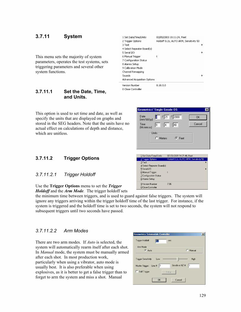
129
3.7.11 System
This menu sets the majority of system parameters, operates the test systems, sets triggering parameters and several other system functions.
3.7.11.1 Set the Date, Time, and Units.
This option is used to set time and date, as well as specify the units that are displayed on graphs and stored in the SEG headers. Note that the units have no actual effect on calculations of depth and distance, which are unitless.
3.7.11.2 Trigger Options
3.7.11.2.1 Trigger Holdoff Use the Trigger Options menu to set the Trigger Holdoff and the Arm Mode. The trigger holdoff sets the minimum time between triggers, and is used to guard against false triggers. The system will ignore any triggers arriving within the trigger holdoff time of the last trigger. For instance, if the system is triggered and the holdoff time is set to two seconds, the system will not respond to subsequent triggers until two seconds have passed.
3.7.11.2.2 Arm Modes There are two arm modes. If Auto is selected, the system will automatically rearm itself after each shot. In Manual mode, the system must be manually armed after each shot. In most production work, particularly when using a vibrator, auto mode is usually best. It is also preferable when using explosives, as it is better to get a false trigger than to forget to arm the system and miss a shot. Manual
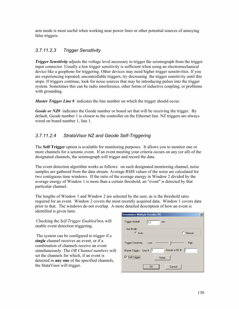
130
arm mode is most useful when working near power lines or other potential sources of annoying false triggers.
3.7.11.2.3 Trigger Sensitivity Trigger Sensitivity adjusts the voltage level necessary to trigger the seismograph from the trigger input connector. Usually a low trigger sensitivity is sufficient when using an electromechanical device like a geophone for triggering. Other devices may need higher trigger sensitivities. If you are experiencing repeated, uncontrollable triggers, try decreasing the trigger sensitivity until this stops. If triggers continue, look for noise sources that may be introducing pulses into the trigger system. Sometimes this can be radio interference, other forms of inductive coupling, or problems with grounding. Master Trigger Line # indicates the line number on which the trigger should occur. Geode or NZ# indicates the Geode number or board set that will be receiving the trigger. By default, Geode number 1 is closest to the controller on the Ethernet line. NZ triggers are always wired on board number 1, line 1.
3.7.11.2.4 StrataVisor NZ and Geode Self-Triggering The Self Trigger option is available for monitoring purposes. It allows you to monitor one or more channels for a seismic event. If an event meeting your criteria occurs on any (or all) of the designated channels, the seismograph will trigger and record the data. The event detection algorithm works as follows: on each designated monitoring channel, noise samples are gathered from the data stream. Average RMS values of the noise are calculated for two contiguous time windows. If the ratio of the average energy in Window 2 divided by the average energy of Window 1 is more than a certain threshold, an "event" is detected by that particular channel. The lengths of Window 1 and Window 2 are selected by the user, as is the threshold ratio required for an event. Window 2 covers the most recently acquired data. Window 1 covers data prior to that. The windows do not overlap. A more detailed description of how an event is identified is given later. Checking the Self Trigger Enabled box will enable event detection triggering. The system can be configured to trigger if a single channel receives an event, or if a combination of channels receive an event simultaneously. The OR Channel numbers will set the channels for which, if an event is detected in any one of the specified channels, the StataVisor will trigger.

131
The AND Channel numbers sets the system such that an event must be detected on all of the monitoring channels in order for the StrataVisorTM to trigger.
Time window 1 specifies the length of the first (earlier) time window. The unit of time length is Noise Blocks, which is 40 times the sample interval. The string to the right of the entry ("=xxx ms", in the above picture) will tell you how long this is in milliseconds when a value is entered. Time window 2 specifies the length of the second (most recent) time window. The Ratio is the threshold value for the average RMS noise in Window 2 divided by that in Window 1 required for an event. The larger the ratio, the larger the event must be in order to cause a trigger. Once the Seismic Controller Software has determined that a suitable event has been detected, a trigger is generated in one of two ways depending on the setting of the next radio boxes:
o If Trigger Via Network is selected, when an event is detected a command is sent over the network to the Geode designated as the master trigger device, which triggers all other Geodes are simultaneously. This method works well when precise absolute time accuracy is not required as the shot record is recorded and time stamped using the local PC clock
o If Trigger via RS-232/GPS) is selected, a byte is immediately sent out the RS-232 port
of the PC control device. This byte is to be used with an external device to generate a trigger pulse known precisely in absolute time. Geometrics provides an exact timing device that AND’s the output byte from the controller with a 1 pps pulse from a GPS receiver. This external device generates a pulse used to trigger the Geodes at a time known with absolute accuracy by the GPS. The GPS then sends this absolute time back to the PC controller via the RS-232 port, where it is read and used to time stamp the record. This method, in combination with an appropriate pretrigger time, permits the
132
collection and accurate time stamping of an event for earthquake recording, crustal refraction surveys, or surveying where time of event is required.
Note: It is advisable to use a negative trigger delay (pretrigger memory) in order to ensure that the onset of the event is recorded. Otherwise you risk missing some of the desired data. Also, in most monitoring applications, AutoSave should be enabled and the Stack Limit should be set to 1.
3.7.11.2.5 Self-Triggering, Detailed Description Geometrics seismic event detection software allows you to monitor one or more channels for a seismic anomaly. If an event meeting your criteria occurs on any (or all) of the designated channels, the seismograph will trigger and record the data. On each designated monitoring channel, noise samples are gathered from the continuously recorded data. Average RMS values are calculated for two adjacent contiguous time windows. If the ratio of the average energy in Window 2 divided by the average energy of Window 1 is more than a certain threshold, an "event" is detected by that particular channel. This method similar to the ‘STA/LTA’ algorithm used in earthquake monitoring. The lengths of Window 1 and Window 2 are selected by the user, as is the threshold ratio required for an event. The system can be configured to trigger if a single channel receives an event, or if all of a set of channels receive an event simultaneously. Combinations of channels can be used to detect specific events or eliminate false triggers. • Events detected on designated ‘OR’ channels will trigger the seismograph when any one of the specified channels sees an anomaly.
• Events detected on designated ‘AND’ channels will trigger the seismograph when all of the specified channels see an anomaly.
Once an event is detected in the decimated data stream, a command is sent to start the seismograph recording at a user defined sample rate and record length. Some variation in the process exists between models. The StrataVisor NX uses an external trigger box. The Geode/NZ recorders require no external hardware. All boards trigger simultaneously with no delay. Once a trigger is generated, the appropriate data in the A/D cards (possibly including data from before the event was identified) are transmitted to the seismic control PC and stored in a user-defined format. A time stamp is added to the data either by the PC, or by an optional external GPS if greater accuracy is required. Once this process is complete, the seismograph returns to its armed state and continues to monitor the decimated data stream, ready to trigger again when an anomaly is detected.

133
Geometrics StrataVisor and Geode seismographs collect data continuously at the system’s maximum sample interval. Data are temporarily stored on the A/D cards in memory that is configured as a circular buffer. These data are transmitted to the seismic controller PC in two ways, either as
• a decimated continuous stream of data used for event monitoring purposes • a seismic data file at a user defined sample rate and record length, sent in
response to either a hardware or software command
The decimated continuous stream of data can be used to measure the output from the sensors attached to the system, almost in real time. Geode/NZ data are decimated as shown in the table opposite. StrataVisor NX data are decimated to 40 samples per second. Once an event condition is detected in the decimated data stream, a command is sent to the A/D cards to send the more densely sampled data at a user defined sample rate. This is possible even though some time has passed because earlier data are still in the circular buffer and can be retrieved before they are overwritten by more recently sampled data. The amount of data sent before the event was detected is determined by a ‘pretrigger’ recording time, set by the operator. The continuous decimated noise data used to detect an event are partitioned into 40 sample ‘blocks’ to make computation easier and demand less resources from the CPU. Two adjacent windows are constructed from these noise blocks and the RMS values from each noise window are calculated and compared. If the ratio between these windows exceeds a user defined threshold, a trigger command is generated for the A/D cards to send the more densely sample data, as specified by the required sample rate and record length. The threshold calculation is undertaken on all channels, and these channels may be compared using AND or OR Boolean logic, as dictated by the requirements of the survey. This threshold calculation is repeated on all channels each time a noise block is received from each channel. When using AND channels to trigger, the length of the W1 and W2 windows should be sufficient so that the event being measured exceeds the threshold value for a long enough time period for
Sample Interval (usec) 3.7.11.2.5.1 Decimation
Factor
Block Length
(ms) 20.83 240 200 31.25 160 200 62.5 80 200 125 40 200 250 20 200 500 10 200
1000 5 200 2000 2 160 4000 1 160 8000 1 320
16,000 1 240

134
the event to be registered as detected in other monitoring channels as well. If this condition is not met, a trigger will not be generated even though all channels may have detected the event individually at different times. This is particularly true for events that do not excite the sensors simultaneously. Detection of non-simultaneous events can be partly improved using the “Minimum Number of Channels” box setting. If this is set to be less than the total number of channels, then the system will trigger without all AND’d channels detecting an event. Note that an appropriate sample rate should be chosen since it effects both the decimated noise sample rate and the final record sample rate. With an incorrect sample rate, it is conceivable that higher frequency events may be aliased and not be detected. Consult the decimation chart above to minimize this effect. In addition, some short time periods may occur between noise blocks where no data are transmitted. GPS Time Stamp for Self-Triggered Data If an accurate time of trigger is required, Geometrics provides a GPS and trigger synchronization circuit to time stamp each record, accurate to a few microseconds. The system is composed of the following parts: • GPS clock • Trigger synchronization box • Seismic recorder (Geode, NZ or NX) • Control computer The system functions as follows: 1 - The GPS provides a continuous 1 pulse per second pulse train to the in put of the trigger synchronization box.
Window 2Window 1
Window 2Window 1
Window 2Window 1
Window 2Window 1
Window 2Window 1
t = 0
t = 30
t = 60
t = 70
t = 80
Window 1 RMS = 10Window 2 RMS = 50
Window 1 RMS = 10Window 2 RMS = 100
Window 1 RMS = 13Window 2 RMS = 100
Window 1 RMS = 17Window 2 RMS = 100
Window 1 RMS = 20Window 2 RMS = 100
Time sequence progression of the detection of an event.

135
2 – when an event is detected from the decimated data stream by the PC control software, an enable command is sent out the RS-232 port to the trigger synch box. This allows the next GPS pulse to be transmitted from the synch box to the hardware trigger input of the seismograph, which triggers the seismograph at a precisely known time. This known time, generated by the GPS, is simultaneously sent via the RS-232 port to the seismograph control software, where it is included in the data header. To enable the external GPS trigger via the trigger synchronization box, select the ‘Trigger Via RS-232/GPS’option on the self-trigger dialog box.
3.7.11.2.6 Continuous Recording Geode/NZ seismographs are also capable of recording continuously at some sample rates. Data are cut into appropriate sized files dictated either by software settings or by an external pulse train, typically supplied by a GPS for accurate time stamping. Contact the factory for more discussion of this option.
3.7.11.3 Test
3.7.11.3.1 Run Analog TestMGOS Analog testing currently requires a Geometrics external test box capable of producing high accuracy waveforms. Software built into the Geode and NZ systems coordinate the acquisition of these signals and perform an analysis for a variety of tests, as specified by user selectable scripts. Testing is fully automatic and provides two types of reports. The first is a summary including specific information regarding failures. The second, more detailed reports provides specifications on a channel by channel basis and can be several pages long.

136
‘Please refer to Geometrics test box manual for specific instructions.
3.7.11.3.2 Geophone Test MGOS The StrataVisorTM and Geode systems are capable of sending a voltage pulse out the geophone inputs to evaluate geophone performance and to test for cable problems. The resulting waveform is captured and analyzed by the StrataVisorTM for the operator to take corrective action. The test is repeated continuously at 2-second intervals to monitor changes in line conditions to see if the corrective action has been successful. Beginning the geophone test will display the following window:

137
Two types of analysis are performed on the recorded waveforms from the line pulse test, and are shown graphically as two sets of bar graphs on the Geode/StrataVisorTM display. The first test (shown by bar graphs A and B) is known as the ‘match’ test and the second test (graphs C and D) is the ‘noise’ test. The analysis begins by first calculating a ‘median’ response of the captured waveform. After eliminating data from obvious open or shorted traces, a relative measure of how the median response compares with each trace is presented in the top bar graph (A). The standard deviation of the last 5 tests is shown in the inverted bar graph directly underneath (B). The noise test is performed by creating a first derivative median trace, and comparing it to the first derivative of the other traces in a similar fashion. The results of each test are presented in the top graph of the bottom set of bar graphs (C). The standard deviation of the last 5 tests is shown in an inverted bar graph directly underneath (D). Open geophones or cable breaks are shown as dashed bars. Bad or noisy phones show responses on either the match (top set) or noise (bottom set) of bar graphs. Sticking or broken phones in strings of geophones are more subtle and show up more clearly in the deviation (inverted B or D) bar graphs. A dialog line is shown at the top of the graph with the match and noise values for each channel. Using the left and right arrow keys moves between individual channels and displays the corresponding analysis. The test is terminated when the CLR key is pressed, and the operator can then print a hardcopy of the results by pressing ENTER or abort by pressing CLR again. The Geode/StrataVisorTM display then shows the trace data from the last test, which can be scaled and printed and saved for visual inspection of geophone impulse response. Some experience may be necessary to recognize faults and bad geophones. Note that this is a relative technique and does not provide quantitative information about geophones. This is not

138
possible due to differing line lengths and geophone configurations. Suspected bad strings and cables can be located with the StrataVisorTM line test and then verified quantitatively with a certified geophone testing instrument. Note also that the statistical analysis identifies geophones that are different from the average; that doesn't necessarily mean a geophone is bad. A perfectly-functioning 40 Hz geophone would therefore be flagged by this test if the rest of the geophones in the line are 14 Hz.
3.7.11.3.3 Update Acquisition Board Bios (LOADER) NOTE: This is a dangerous process and you may damage your Geode system. Contact the factory, and read this documentation carefully to make sure that you really need to undertake this procedure. Follow all steps exactly. Failure to follow these procedures make result in alteration of the Geode/NZ firmware that can only be fixed by returning the instruments to the factory. The firmware loader is a part of the Geode acquisition board that resides in flash memory. It is never lost by power down. The loader program runs like BIOS in a PC. It is the boot load code that talks to the controller and loads the Geode operating system code each time the Geode acquisition board is powered up. Geometrics may upgrade this code to provide new features and commands between the controller and the Geode acquisition board. Contact Geometrics periodically or check our web site for announcements of upgrades The software included in MGOS burns the firmware with a new version of the Geode internal operating software. All Geodes and all lines are updated at one time. Note: If you have firmware version lower than 2.5 or lower, do not use this option to burn the Geode firmware. Version 2.717 and lower generally coincides with Geodes with the
GREEN power button on one side. Contact customer service for advice on how to burn this Geode or NZ
If you have firmware version 2.5 or higher, your can procede with using this software to upgrade your firmware. Check the firmware from the SYSTEM>VERSION NUMBER option, and check the LOADER SOFTWARE VERSION to determine the firmware version.

139
Note: We strongly recommend that you contact the factory and talk with customer service before proceeding with burning your firmware. This is a dangerous process and you can damage your system resulting in a factory return. When done properly this is a safe procedure, but should not be done unnecessarily.
3.7.11.3.3.1 Downloading and Burning New Geode Software Please follow all steps exactly as shown: 1) Download updated flash loader firmware from the FTP site on the Geometrics web site. The
file will resemble the following: (Flash2_714&2_41.exe). The numbers will be different and depend on the version of the flash loader. This example has placed the flash loader on a floppy disk drive, which resides in the A: drive on the controller.
2) From the SYSTEM>TEST menu, select Update Acquisition Board Bios (LOADER) from
the test menu.
3) Read the warning screen carefully and follow any cautions outlined in the message.
Do Not Remove the Power Cable from the Geode or NZ while Updating the Firmware

140
4 ) Click on I Agree to proceed. 5) The dialog box opposite will appear. Use the browse button to select the firmware version that you have downloaded from Geometrics web site. Remember, it should be version 2.718 or above. 6) Press the Start Burning button. You will be asked to confirm the burning when presented with another dialog box. Once confirmed, the following dialog box will appear and burning will start. A countdown timer will show the duration of the burning process. Note: do not remove power from the NZ or Geode while the burning is taking place. 7) A dialog box will be displayed indicating the estimated burning time remaining.

141
8) Once burning is complete, the following dialog box will appear:
If the power LED on the Geode is blinking rapidly, burning is taking place. If the LED is blinking 3 seconds on and 1 second off, burning has been successful. If there is no blinking, its time to call Geometrics! Burning must be undertaken at the factory. Exit the program to close the software. 9) Turn off all of the Geodes by disconnecting the power cord. Turn them back on by plugging them back in and making sure that the power button is pressed. The next steps will check to see if all the boards in the Geode were properly programmed. 10) When the program is running click on the <System> pull down tab. 11) From the System pull down screen select the Version number. Check each Geode board version by using the arrow keys >> or << to move between board sets. There are 8 channels per board. This example has only one acquisition board set. 12) If all went well, you are done.
Do NOT Remove Cable or Power From Geodes YET.

142
This is one possible error that may be seen if the Geode is not properly connected to the Controller. In case of this type of error check your Geode connections. Make sure it has power. Make sure the Link light is on. Go back to the beginning and restart the process. 13) If the Geode is not responding after a Flash update, even after a power down and back up, call Geometrics Customer service.
3.7.11.4 Enabling Repeaters and Disabling Acquisition Cards MGOS Geode and NZ A/D board sets house 8 channels each. Up to 3 board sets (24 channels) can be in each Geode module and up to 8 board sets can be in each StrataVisor NZ. It is possible to turn off the A/D function so that each board sets simply acts as a repeater and passes data on to the next active board set. This function is handy if you wish to extend the distance between active, acquiring Geode modules, or if you simply wish to remove some channels from your system as if they were not there at all. For example, if you were using 24 channel Geodes and wished to extend the distance between active recording Geodes, you could enable all boards in the units between active Geodes and double the transmission distance.
To enable this option, choose “Select Repeater Board(s) from the system menu shown opposite. You will immediately be presented with an additional menu indicating that the MGOS seismograph program will automatically restart after you have made your selection in the following menus. The program needs to be restarted as system settings in the Geodes are enabled at a very low level and this is only done at startup.
After choosing yes, the following menu will appear: A field is shown for each line that the system found on startup. In each field, you can enter

143
the number of the board set that you wish to have enabled as a repeater. Remember, the board set and its associated channels will essentially disappear, and not be available again until these settings are changed. Note that you can specify a range of boards (3-8) or individual boards, separated by commas. If you wish to have these settings enabled you must check the box labeled “Enable Repeater Mode” before the setting will take place. When you click on the OK button, your system will restart, enabling repeaters and active channels as you have specified. There are other combinations of disabling channels, depending on your field situation and cabling. For example, if you own 24 channel Geodes and own 8 channel cables for larger scale surveys, you may wish to enable the last two board sets in each Geode as repeaters. Note that repeater mode differs from the menu setting in the ACQUISITION menu to simply disable channels. Disabled channels can be turned on or off at any time and in combinations other than in 8 channel groups.
3.7.11.5 Serial I/O MGOS Facilitates data communication between the seismograph and other external serial devices like vibrators, guns, navigation systems and streamers. Geode/StrataVisor systems can either send data to other devices or receive data that is automatically integrated into the header of the seismic data.
Choosing the Serial Input fly-out option presents the following menu:
Choose the settings that pertain to the configuration that you are operating, by selecting the COM port, parity, stop bits and whether you want the end of a string recognized as a carridge return (CR) or a line feed (LF). You also have the choice of concatenating several strings or simply storing a single string. Settings for a downhole Durant counter are also included. Note that if you have a GPS receiver attached, you must check the Replace PC time Stamp with GPS Time checkbox to use the GPS time. Some customization may be required for non-standard devices. Please contact Geometrics to discuss your requirements. Remember to make this option work, you must check the ‘Serial Input Enabled’ box.

144
Serial output works in much the same way. Selecting the serial output flyout yields the following menu:
When serial output is enabled and the OYO compatible radio button selected, the file number, tape, number of active channels is sent out the selected serial port. This option is often used when passing information to a navigation system.
3.7.11.6 Manual Trigger The Manual Trigger utility is used to trigger and record data from the keypad, without the need for an external trigger source. This is useful for testing or recording background seismic noise. The manual trigger is almost never used to record real seismic data, since analysis depends on exactly synchronizing the seismograph with the energy source.
3.7.11.7 Configuration Status
3.7.11.7.1 Configuration Status Menu The configuration status option allows you to query the status of all Geodes and all individual board sets on each line

145
The configuration status menus contain a great deal of information that indicates how your system is operating. The system is checked every few seconds to determine whether all
operations are normal. The top of the menu indicates which line number, which Geode and which board set are currently being interrogated. You can click on the right and left arrows in opposing corners of the menu to view the status of other Geodes and board sets. There are many items that pertain to debugging the system if there are difficulties, but some of the more important settings deserve additional explanation: Battery Voltage: Indicates the voltage of specified board set in specific Geode. Note that all board sets in each Geode should
indicate roughly the same voltage. If the battery voltage drops below 10.4 volts, a warning will be displayed. If the voltage drops further below the 9 V critical level, an error is reported. Ethernet 1 Connection: Indicates whether the downstream connector on the Geode (arrow out of the circle) that sends data back to the controller or downstream Geode. If this connection is backwards, a warning is displayed. Ethernet 2 Connection: Indicates whether the upstream connector on the Geode (arrow into the circle) is connected to the downstream connector of the previous Geode (arrow out of the circle). If this connection is backwards, a warning is displayed.
Ethernet 1 and 2 Link: Tests to determine if the digital interface between Geodes is working properly in the upstream and downstream directions. Acquisition Board Position: If there are more than 8 channels in a Geode, this indicates the A/D board position in the board stack. Master Trigger: Displays whether this board set has been enabled as the master trigger. The remaining parameters show verification of acquisition parameters and other system settings.

146
3.7.11.7.2 Error Conditions Shown By the Configuration Status Menu If an error condition occurs, the configuration status dialog box automatically pops up and displays the status of the Geode board set that caused the error. Since there are many parameters to check, the specific error(s) is located at the top of the screen between the square brackets […..].
Shown in the opposite menu is an error condition caused by disconnecting the line between two Geodes. Note the white ‘X’ circled with red to indicate a critical error. The system correctly identifies where the error has occurred and suggests a solution. If the error is located further up the line, an X error symbol is located next to the right arrow. If the error is closer to the controller, the arrow is located on the left. Pressing the appropriate arrow button pages to the Geode indicating a fault condition.
Some error conditions are not as critical and only a warning triangle is shown. These errors can often be fixed without restarting the line. Some errors are simply annoyances and can be defeated if they are showing frequently. For example, the system will first start warning you of depleted batteries when their voltage reaches 10.4V. If you wish to ignore this warning and continue surveying, you can check the appropriate dialog box on the bottom if the configuration status menu, shown below.

147
3.7.11.7.3 Signaling at a Specific Geode If you wish to indicate to your field crew that they should investigate a particular Geode, you can press the “Blink This Board Power Led for 15 Sec” button to start a rapid pulse blink on the indicated Geode. This menu option is shown above. You can use the left and right arrow keys to select other Geodes. Newer versions of Geodes also have a beeper in the Geode box which gives an audible indication of where the box is located.
3.7.11.8 Alarms The Geode/NZ system has a series of alarms that can be used to alert the operator of error and warning conditions. Warnings can be audible or visible. Most are self-explanatory. All can be defeated either through this menu system, or interactively when the warning dialog box appears. Critical errors like overdriven channels and tape errors are written to the log file. You will see only the alarms enabled by the options that you have purchased with your software, as some alarms are specific to marine, self-triggering or monitoring applications. Some alarms will write a status message to the survey log file, and others, like Report Self-Trigger Shot, will display a special dialog box designed to get the operator’s attention

148
Digital cable
3.7.11.9 Calibration Mode Geode/NZ acquisition boards are self calibrating to remove DC offset. This maintains the dynamic range of the system and allows simultaneous measurement of small and large signals. Calibration takes approximately 2 seconds. There are some situations when it is desirable to defeat the calibration, for example if you are stacking very quickly, or if you are doing marine surveys where the inter-shot times need to be small. By choosing to calibrate every nth saves, you can ensure periodic measurement appropriate to the kind of survey you are undertaking. Also by keeping the temperature of the instrument stable, you can minimize the need for calibration.
3.7.11.10 Channel Remapping Channel remapping allows you to change
1. the order of channels on each analog spread cable that connects to the Geode
2. reorder the Geode boxes.
You would use this option if your cables were wired opposite to the default order normally used in Geometrics wiring, if you wished to turn your line around to have the low channels at the opposite end, or if your cables had a wiring error. Channel remapping is also often necessary when using more that a single network cable.
3.7.11.10.1 Default cable wiring of Geometrics seismographs Default order is defined as the natural electrical order in which channels are oriented when the system first powers up before remapping. Refer to Section 3 under Connector Wiring that discusses standard wiring configurations. You may have requested a custom wiring configuration from Geometrics. If you are confused about your wiring, contact the factory and refer to the serial number and job number.
Geode cables are typically wired in a ‘high-side configuration’, meaning that the Geode connects closest to the highest numbered channel on the analog cable. The

149
figure above shows this configuration for a single box system, with 24 channels.
3.7.11.10.2 Multiple Geodes The following diagram shows a default single digital line (one network card) system with 3 Geodes. Note that Geode one is always closest to the controller in a default configuration.
3.7.11.10.3 Multiple Network Lines The next diagram below shows a default configuration with two digital lines (two network cards) with the controller positioned in the middle. Line 1 is on the left and line 2 is on the right. One might use two lines to increase data throughput to reduce time between shots. Like the configuration above, the Geodes are numbered starting closest to the controller. The seismic controller software labels all of the channels contiguously even though they are on two separate digital lines. However, if the lines are collinear, the first line will have the channels ordered backwards. This can be easily rectified with the remapping feature.
There are two ways of remapping channels: automatic mode and manual mode. Automatic mode settings are listed on the top of the remapping dialog box, and manual mode on the bottom.

150
Reverse Geodes
Reverse Cable
3.7.11.10.4 Automatic Channel Remapping Automatic channel remapping allows you to reverse either the order of the Geodes on the line, or
reverse the order of the channels on the spread cable. The above diagram shows the result after both channels and Geodes have been reversed, renumbering the line so that low channels start on the left hand side and increase towards the right. In the dialog box, the automatic remapping boxes referencing line 2 remain unchecked, since the default orientation on line two was correct.
3.7.11.10.5 Manual Channel Remapping Channels can be remapped on an individual basis using the Manual Map Mode. Select the appropriate check box, and enter the order in which you would like the channels that differs from the default order. You can specify individual channels separated by a comma (1, 3, 4, 6 etc) or a range of channels (1-13, 24-14 etc). For example, if you wanted the channels ordered backwards on a 24-channel system, you would enter 24-1. If you wished to reverse the order of channels 1-12 in a 24 channel system, you would type 12-1, 13-24. Other examples are shown opposite, and are available by pressing the See Examples button on the remapping menu.

151
3.7.11.11 Sounds The Geode/NZ system has several sounds to alert the operator of the progress of his survey. These sounds can be changed or defeated, if required.
The dialog box opposite shows the situations in which sounds are generated. Options can be defeated or reselected by clicking on the menu item.
3.7.11.12 Advanced System Options You may need to take advantage of some advanced system settings if you are undertaking specialized surveys that require continuous recording or very high sample rates.
3.7.11.12.1 Enable ADC High Pass Filter Uncheck this option if you have modified your Geode hardware for low-frequency option (either 0.6 Hz low cut or DC operation). Note that there may be implications for testing your system with Geometrics internal or external testing hardware.
3.7.11.12.2 Enable Subsample Trigger Synchronization
This option shifts the data stream to ensure that trigger accuracy of 1/32 of a sample interval is obtained. This is particularly important when data are to be stacked as it ensures excellent synchronization of the trigger. If you required exact synchronization to a GPS trigger during continuous recording, the box should be checked.
3.7.11.12.3 Enable Continuous Acquisition Allows Geode or NZ to record data continuously. See section 7 for additional settings that accompany continuous acquisition

152
3.7.11.13 Version Number Selecting Version Number displays the above window. When reporting software problems, please be able to supply the software version number.
3.7.11.13.1 Changing registered options. There is also the ability under the Version Number menu to add or remove additional software options that you may have purchased. In this menu you can also view the options that come standard with each package and any existing options you have already purchased.
3.7.11.14 Close Controller Close Controller will close the seismic controller software. If you are operating from a separate PC or laptop, it will return you to the desktop. If you are using the NZ, it will shut down Windows. If you are operating remote power up/down Geodes from your laptop and wish to shut the entire line down and turn off the power, you should first place the toggle switch on your network interface box to the Enable Power Down position.
If you fail to place the toggle switch in the Enable Power Down position, all Geodes and boards will shut down, but the first board in the line will be left powered up, draining power from the
Enable Power
Up
Enable Power Down
Battery Test

153
battery if left overnight. You can rectify this problem without restarting the controller by simply disconnecting the battery momentarily. If you have Geodes connected directly to an NZ/C II-IVor NZC controller without the network interface box, shutdown of all Geodes, including the first one, will be automatic.

154
3.8 The Geometry Graphical User Interface The Geometry GUI provides a graphical representation of your survey, along with a wide range of control capability. It is particularly useful when conducting reflection surveys, but can be useful in a wide range of applications. It summarizes, in one simple view, the physical positions and other attributes of the hardware on the ground, and allows graphical control of these. 3.8.1 Visual Attributes Below is a typical display of a 96-channel, four-Geode layout. We will first describe the display itself, and follow with a description of its control capabilities.
The information in the display above is summarized below. Where appropriate, the actual setting, as shown above, is shown in brackets for reference.
Scale (x1 shows entire spread, ranges to x100 – this is also a drop-down menu).
[Green] Active (data) channel. Triangle pointing down indicates low gain, up indicates high gain.
[Grey] Inactive (data) channel (low gain, high
gain).
[Maroon] Aux channel (low gain, high gain).
[Violet] Pilot channel (low gain, high gain).
[Light green/dark green] Active channel (low gain, high gain, frozen).

155
[Grey/blue] Inactive channel (low gain, high gain, frozen).
[Maroon/blue] Aux channel (low gain, high
gain, frozen).
[Violet/blue] Pilot channel (low gain, high gain, frozen).
Geode module (active/inactive/warning/error, with number of channels indicated).
13.9V 10.9V 9.9V
Battery (good/low/bad, with voltage indicated).
Shot location (double-click to change icon, drag to desired location)
PC controller location (double-click to change icon, drag to desired location).
Flag marking beginning or end of spread or beginning or end of active portion of spread. Labeled with shot offset (top) and flag location (bottom). (double-click to change flag style).
Trigger cable (orange)
Geophone (analog) cable (black).
Network (digital) cable (blue).

156
SHOT LOC [162.00]: The shot location is indicated by the position of the yellow truck and is labeled in red. The red line is the trigger cable and indicates which Geode you have plugged the trigger into (master Geode). OFFSET [62, 108, 578, 888]: The beginning and end locations of the spread, along with the beginning and end locations of the active portion of the spread, are indicated by a flag. The distance between the shot and the flag, or shot offset, is shown immediately above the flag. LOCATION [100, 270, 740, 1050]: The location of each flag is indicated immediately below the flag. TRACE # [1,2,3…96]: The trace number represents the position of the trace in the shot record, from 1 to n, where n is the number of channels. This number will always increase from left to right. Trace numbers corresponding to flags are shown in red. CHANNEL #:The channel number indicates the physical channel number within the Geode module. With most systems, no distinction is made between the channel number and the trace number. However, as we will see later, the StrataVisor/Geode allows you to map the channels any way you wish via software to accommodate any geophone cable configuration. If no channel mapping is done, the trace number and the channel number will be the same. Generally, the channel number need not be displayed, but it can be useful in the initial mapping of your channels if this is necessary. Channel numbers corresponding to flags are shown in red. CHANNEL #: The second channel number label refers to and is in line with the channel numbers on the Geode modules, and represents the channels that they are connected to. GEODE # [G2, G1, G1, G2]: Each Geode on each network line is numbered automatically. The Geode closest to the controller, vis-à-vis network topology, is always Geode number 1. In the above example, we have two separate networks, so there are two each of G1 and G2. BATTERY LVL [13.9, 13.8, 13.9, 13.8]: This indicates the battery level for the Geode. LINE # [L1, L2]: In the case of more than one network line, as above, the Geode software will automatically assign one to be Line 1 and the other to be Line 2. This assignment is arbitrary but consistent: the designation of the network ports on your PC will be the same with each session. PC LOCATION (see above) [660.00]: This shows the location of the PC controller. For convenience only. 3.8.2 Control Functions Various survey parameters can be controlled via the Geometry GUI. Right-clicking the mouse will bring up different menus, depending on where your pointer is at the time.
3.8.2.1 Shot location Right-clicking on the shot icon will display the following menu:

157
Choose “Enter Shot Location” to display the Geometry menu and type in the shot location:
Enabling the “Set Shot Location at Mouse Cursor Location” toggle switch allows you to set the shot location by simply pointing and clicking at the location you wish to move the shot to. Note: At any time, you may click and drag the shot icon to the desired location. Finally, clicking on “Select Next Shot Location Symbol” will change the icon used to indicate the shot. For instance, to say screen space, you may choose to use a simple asterisk:

158
Note: Double-clicking on the shot icon will cycle through the various choices.
3.8.2.2 Geometry Tool Bar Display Setting Right clicking on the white portion of the display will reveal the following menu:
The first eleven choices in the above menu are discussed elsewhere in this manual. Choosing any one of them directs you to the appropriate menu or, in the case of channel roll, takes the specified action. Click on any item to review: Group Interval, Group/Shot Locations, Phone Increment, Shot Increment, Gap, Channels Auto Roll, Roll Channels Up, Roll Channels Down, Freeze Channels, Specify Channels, Channel Remapping. You may choose which information to display on the Geometry GUI by clicking on “Geometry Tool Bar Display Setting”, which will reveal the follow menu:

159
Using the above menu, you may de-select items to simplify the GUI and save screen space.
3.8.2.3 Select Geophone Cable Type For purposes of display, and for mapping channels correctly, there are three basic cable types. In order for the geometry display to match what you have on the ground, you must indicate what kind of cable you have. Click on “Select Geophone Cable Type” to display the following menu:

160
A “high end” cable means that channel 1 is connected to the furthest geophone from the Geode module:
A “low end” cable means that channel 1 is connected to the closest geophone to the Geode module:
“A split spread” cable consists of two cables, with the Geode in the middle:

161
Choose “mixed” geophone cable if you have a combination of those described above, and your survey layout will be displayed as follows:
3.8.2.4 Zoom Click on “Zoom” to display the choices of scale, and choose the desired scale. Note that you can control the scale with the zoom selection box in the upper left hand corner of the Geometry GUI, as discussed in Section 4.8.1. However, it is included in this menu in the event you choose not to display zoom selection box. Note: You may also control the scale by highlighting the zoom control box and using the left and right arrow keys. Also, the “Page Up” key will set the zoom to x1, and the “Page Down” key will set the zoom to x100.

162
Note: A zoom setting of x1 will result in the entire survey layout fitting within the visible portion of the GUI.
3.8.2.5 Dock The Geometry GUI is a “dockable” toolbar. Generally, it is “docked” or “fastened” to the bottom of the display. However, if you would like to move it to another location, you can “undock” it and move it around like any other window. You may close it by clicking on the “X” in the upper right-hand corner. To bring it back, open the Window menu, and click on “View Geometry Tool Bar”. Note: Since the Geometry GUI is a toolbar rather than a window, it will always be on top.
3.8.2.6 Geode Status Right-clicking on a Geode module will display the following menu:

163
This is the same as “Configuration Status” in the system menu.
3.8.2.7 Ping Geode If you have remote power-up Geodes, you may “ping” it – it will emit a high-pitched beep for 15 seconds. This can be useful when troubleshooting the line.
3.8.2.8 Set Geode as Master Trigger You may set any Geode to be the master trigger Geode. The trigger line (red) will connect the source to the master Geode.
3.8.2.9 Select Geophone Cable Type This is covered above in Section 4.8.4.
3.8.2.10 Disable Data Channel Right-clicking on a geophone symbol(s) will reveal the following menu:
If the channel is not an aux or pilot channel, clicking on “Disable Data Channel (Not Pilot or Aux) will make that channel inactive. Changing channel attributes is also discussed in Section 4.7.4.5.
3.8.2.11 Enable Channel If a channel is currently inactive, clicking on “Enable Channel” will activate that channel as a data channel.
3.8.2.12 Set Channel to High Gain The Geode/NZ normally ships in a configuration giving you the choice of selecting the lower or higher of two analog gains (12/24 dB or 24/36 dB). Choosing “Set Channel to High Gain” will set that channel to the higher of the two.

164
3.8.2.13 Set Channel to Low Gain Similar to above, choosing this option will set the channel to the lower gain of the two.
3.8.2.14 Scrolling If you set the zoom factor to a number larger than one, you may scroll the image left and right. There are three ways to scroll. You may:
1) Use the scroll bar. 2) You may highlight the scroll bar and then use the left and right arrow key. 3) You may place the pointer at the right or left edge of the display. An arrow will
appear (see below), and the display will scroll with each click of the mouse. This is particularly useful if you have elected not to display the scroll bar.
3.8.2.15 Selecting Multiple Channels The same operations performed on individual channels as discussed in Sections 4.8.2.10-13 can also be performed on groups of channels. You may select a group of channels or geophones by using your mouse to draw a box around them:

165
The will be highlighted, as shown below:
If you wish to highlight non-contiguous channels, hold the CTRL button down and click on the desired channels:
If you wish to highlight several non-contiguous groups of contiguous channels, hold the CTRL key down and draw boxes around those you wish to highlight:
In short, holding the CTRL key down allows you to select/deselect a channel or group of channels without affecting the status of the other channels. Experiment with the channel selection function to get a feel for how it works. Once you have selected your channels, simply right-click to display the following menu:

166
You may then change the gain or status of the entire set of selected channels as discussed in Sections 4.8.2.10-13
3.8.2.16 Tool Tips There is not enough room to display the geophone or trace number or its location for every geophone group. To display the information for a particular group, place your pointer on the geophone symbol, as shown below.
3.8.2.17 Channel Remapping Assistance Channel remapping is discussed in Section 4.7.11.10. This can be a somewhat confusing subject, but it is greatly simplified by the Geometry GUI. The key is to choose the remapping parameters and cable types that result in the graphical representation of your survey matching what you have on the ground. This is best illustrated by example. Consider the following 96-channel, two-network line Geode system.
The channels have not been remapped; everything is set to default values (note that the trace number and the channel number is the same for all geophones). The geophone cables are set to the standard “high-side” configuration. If your cables are “high side”, then if you connect everything up as shown above, your traces/channels will be in the proper order -- if you set off a shot to the left of the spread, traveltimes will increase to the right, as shown below.

167
However, let’s assume your cables are not Geometrics “standard”, but are “low-side” cables. This means that the lowest channel number is closest to the Geode module, which is the opposite of that shown above. In this case, if we set off a shot at the left end of the spread as laid out above, our first break times would look like the following:
The Geodes are in the proper order, but each one is flipped. To rectify this, we must do two things: 1) change the geophone cable setting in the Geometry GUI to “low side” cables, after which our Geometry graphic will appear as below, and 2) plug each Geode into the opposite end of the cable.
The second step is crucial: what is on the ground must match what is on shown on the geometry graphic.

168
Compare to the previous geometry graphic; note that it is now the low-numbered channel of each cable that is plugged into each Geode. If you connect everything up as shown here, your shot record should be correctly mapped. In the above configuration, one would probably find it more convenient to place the controller PC in the middle of the Geode spread and connect the networks to the two nearest Geodes, as shown below. This would require less network cable than the configuration shown above.
As before, if you make this change on the ground, you must also make the change in the channel remapping module. In this case, we simply reverse the Geode order in network line 1:
Compare to the previous configuration and you will see that Geode 1 and Geode 2 have been interchanged.

169
To make this a little more understandable, it is instructive to show what your shot record would look like if you made the change on the ground, but did not remap the channels such that the geometry GUI matched the field layout:
Again: The system is designed so that if you make the geometry GUI match what you have on the ground, the channels will be mapped correctly.
170
4 Hardware and Accessories
4.1 Equipment and Accessories for Operation It takes several peripheral accessories to conduct a seismic survey. Besides the seismograph, you will need a power source, geophone cables, geophones, an energy source, plus a few minor items. Specific items vary considerably depending on the survey. Because of the potential variations, only a minimum of the required accessories are supplied with the basic instrument. The remaining accessories may have been ordered with your system as options, or you may have intended to supply your own. Most seismographs have a high degree of interchangability in accessories (particularly geophones and cables), and you may be using equipment you already own. The shipping documents should be checked to confirm the items supplied as standard equipment and those ordered as optional accessories. Geometrics has applications specialists on staff to help tailor your survey instrumentation. 4.1.1 PC Requirements
4.1.1.1 Memory Requirements If you are using a laptop or PC for the Geode control device, some specifications are recommended. The memory requirements for seismic data are significant and in the following guidelines, we have been conservative. Small systems of 24 channels with short memory will run in 64 Mb of RAM, but may be slow. IN general, 256 Mb should be considered standard, whereas large systems of 240 channels and above run best with 1024 Mb of RAM.
4.1.1.2 CPU Requirements As in most scientific applications these days, faster is better. Although we have run small systems on Pentium 90’s running 64 Mb of RAM, we recommend a minimum of a 233 PII with memory as specified above. If you are writing tape, a processor of 1 GHz or faster is recommended. 4.1.2 Power The StrataVisor and GeodeTM portable systems operate from a nominal 12 volts DC. This may be a rechargeable battery pack, a standard automotive battery, 12-volt vehicle power, or an AC-powered, 12-volt DC supply. Current drain of the StrataVisor NZ varies depending on the number of channels and the options installed. The small systems draw about 8 amps, increasing with the number of channels and installed options to nearly 20 amps for the largest systems. Additional power is required for short intervals when the printer is running. The power source selected should be sufficient for a day in the field.

171
Geodes are much lower power devices and use approximately 0.6 W (0.05W) per channel. A 10 amp hour battery should run the Geode for several hours, enough for a single day survey. If you are using the correlator continuously in a high production vibrator survey, a 15 amp-hour battery is more suitable. For cold weather operation, a 15-20 amp-hour battery is recommended. Geodes run in a lower power mode when the seismic controller software is not running. Remote power up Geodes are capable of powering off when idle, reducing power consumption to almost zero. A general purpose power cord with clip connectors is provided with each system. Connect the seismograph to the power source tightly as momentary loss of power will cause the loss of any data in memory and possibly interfere with disk operations. Optional rechargeable gel-cell batteries are available from Geometrics. Battery packs are supplied with an appropriate power cord to connect to the power receptacle plug on the seismograph. Also available with the rechargeable battery is a 110/220 volt AC-powered battery charger. Before using this charger, check and see that the proper AC voltage is selected on the switch. The Geometrics charger is designed to be connected continuously to the battery. The system will charge at a high rate until the battery is charged, then switch to a standby voltage. A light on the charger indicates when the rate switches to trickle charge, which also means the battery is charged. Charging will take several hours. 4.1.3 Blink Codes The blue LED’s that are on the side of the StrataVisor NZ and Geode have several modes which convey information about the device’s status.
Power LED Blink Mode Meaning Not Blinking Not connected or power not on Every 3 seconds Standby Mode Rapid (every .1 sec for 1 second) Download code and reset Every 7 seconds On line, communicating data and instructions Every 0.5 seconds for 15 seconds Can be blinked manually from the
SYSTEM/CONFIGURATION STATUS menu. Note that you must select the first board in each Geode for the power LED to flash.
Ethernet LED Blink Mode Meaning Not Blinking Not connected or not functioning Every 3 seconds Detects Neighbor / in Low Power Standby Mode Every 7 seconds On line, communicating data and instructions 4.1.4 Connecting Geodes To Your Laptop Or StrataVisor NZ
4.1.4.1 Digital Interface Adapters (network adapters) As discussed in earlier chapters , Geodes can be connected to your laptop, to a PC or to a StrataVisor NZ – essentially any PC device that has a functional, industry standard Ethernet port. In standard Category 5 (CAT5) cable that is used for Ethernet data transmission, there are 4 pairs of wires, but only two are used for actual data transmission. Geometrics uses the other two pair of

172
wires for synchronous triggering of all A/D cards and to allow remote power up/down for Geode distributed modules. Geometrics provides Network Interface Boxes (NIB) to connect Ethernet adapters in your PC or laptop to Geode modules. However, since the extra pairs or wires used for triggering or remote start must be used appropriately, Geometrics offers different NIB solutions depending on your application. For a single line of Geode distributed modules connected to a LAPTOP use NIB adapter P/N
0028102-01. This adapter the wires for remote start and trigger disabled so they will not damage the PCMCIA connector in your laptop. This adapter should also be used with a PC network card.
For two Geode lines, use NIB adapter P/N 0028102-02 Cable Adapter. Trigger and remote start disabled back to the laptop but the trigger wires passed between lines. For a single Geode line connected to a StrataVisor NZ via the external RJ-45 connector, use NIB adapter P/N 0028102-03. This NIB has the trigger cable brought out from the internal A/D cards in case the trigger is initiated on the NZ trigger connector. These NZ’s are an older design; modern NZ2’s have the ruggedized Ethernet connector built directly on the side and no separate box is required. The NIB’s will soon be available with a toggle switch used in conjunction with the seismic software to start and shut down remote power up Geodes. Single line NIBs are part number 28102-04 and dual line NIBs are part number 28102-05. The toggle switch has 3 positions
• Enable power up: powers up first board in the line so that starting the seismic controller software will power up the entire line
RJ45 Adapter
RJ45 - 1
Adapter RJ45 - 2
RJ4Adapter

173
• Enable power down: prepares the line for power down prior to shutting down seismic controller software • Battery Test: evaluates the charge on the 9V battery inside the NIB.
4.1.4.2 Digital Cable Considerations Geode digital interface cables are available as either lightweight, or with an abrasion resistant coating. Maximum digital cable lengths are as follows:
o 250 m length between Geodes o 250 m between the first Geode and an NZ with internal channels on the same line o 100 m between network connections on NZ’s with no channels o 100 m between the first Geode(s) and an NZC o 100m between a laptop and the first Geode
Enable Power Up
Enable Power Down
Battery Test

174
4.1.5 Interfacing the StrataVisor NZ to External Devices
4.1.5.1 Connecting Internal PC to an External Network
4.1.5.1.1 Old Style NZ with RJ45 external connector Close the StrataVisor NZ program if it is running.
Open the display panel and look in the area to the right behind the floppy drive. There is a label “NET”. Look just below the label and there will be an RJ45 plug and connector. The plug and gray cable go to the acquisition cards. Remove the plug and use the RJ45 socket for you network connection to another computer. Use a crossover cable to make the connection to the laptop or other computer. Use a straight cable for plugging into a system network connection (a hub connection for instance).
To remove the external network connection, reverse the process by unplugging the network cable. Plug the gray cable (from the acquisition cards) back into the socket marked “NET”.
Acquisition Gray cableAnd RJ45 plug
Display cover
Floppy

175
4.1.5.1.2 NZII systems with multiple external network ports You can Ethernet port 2-4 to access the internal PC directly.
4.1.5.2 Setting up Network Protocol On NZ Internal PC WARNING: Geometrics currently recommends against using TCPIP protocol.
This procedure below allows connecting between your laptop and StrataVisor NZ using “NetBEUI Protocol”. You should connect crossover CAT5 cable between laptop and NZ using the procedure above. Setup for StrataVisor NZ 1. Close NZ program by pressing <Alt>&F4 together. 2. If you don’t know how to connect net cable, follow a document “How to connect to an external network”. 3. From the DESKTOP menu, select “Start”, “Program”, and “Windows NT Explorer” 4. Scroll down to your data file folder and right click it. Click on “Sharing”. 5. Select “Shared As” and click “ok”. Setup for your laptop and connection with StrataVisor NZ 1. From the DESKTOP menu, select “Start”, “Program”, and “Control Panel”. 2. Double click on “Network” and go to “Protocols” tap menu. 3. Make sure you have a “NetBEUI Protocol”. If not, add it. 4. Choose “Adapters” tap menu and click on “Properties” of your Ethernet Adapter. 5. If everything is done, click “ok” or “cancel” depending on your change. You may reboot your laptop. 6. From DESKTOP, double click on “Network Neighborhood” icon. 7. Click on “Controller”. This is a StrataVisor NZ. 8. Now you can see your data file folder. Caution: Some customers have experienced occasional system hangs using TCPIP protocol on the StrataVisor NZ seismograph. We believe we have this issue resolved, but recommend vigilance.
4.1.5.3 Integrating Two StrataVisor NZ Computers for Use as One System
It is possible to control the acquisition channels of one NZ with another StrataVisor NZ. This process is called ‘master/slaving (m/s)’ two NZ instrument together and is described below:
4.1.5.3.1 Configuring the Slave This requires opening the display panel. Look in the area to the right behind the floppy drive. There is a label “NET”. Look just below the label and there will be an RJ45 plug

176
and connector. This gray cable goes to the acquisition cards. Remove the plug and use an RJ45 female to female crossover socket to adapt a network cable that will go to another NZ or Geode output. You can also use a crossover cable and two RJ45 female to female sockets. See Geometrics for an adapter cable that converts the Geode Ethernet connection to an RJ45 plug.
4.1.5.3.2 Configuring the Master NZ
Gray cable and RJ45 plug provides connection to output side of acquisition cards.
RJ45 Female to Female Crossover adapter (or straight through adapter with a crossover CABLE)
This cable connects to either another NZ that will act as a master, or to the end of a line of Geodes. The cable shown here has a Geode connector, but could be an RJ45 if connecting to an NZ.

177
At this point you should connect the other end of the Ethernet cable to the input acquisition connector on the master NZ . The master NZ may have either an RJ45, or a MIL-C-10544 connector its side. Power up both NZ systems. The master NZ should automatically detect the additional boards on the slave StrataVisor NZ, as well as all of its own internal channels. Check to see that this is the case using the SYSTEM/CONFIGURATION STATUS menu item.
4.1.5.4 Connecting a StrataVisor NZ to the end of a string of Geodes
You can connect the acquisition channels in an NZ to up to 4 lines of Geodes to add additional channels. Power down the controller for the Geodes and the NZ to be used as a slave. Follow the procedure above to prepare the NZ as a slave. Connect the cable to the NZ acquisition channels to the input connector on the last Geode in the line (annotated by a connector with an ARROW pointing INTO a circle). Restart the Geode controller. All acquisition channels should be automatically detected. . Check to see that this is the case using the SYSTEM/CONFIGURATION. Modern NZs have either two or four ruggedized network controllers for connecting upto four lines of Geodes. Older NZs have one RJ-45 network connection. Note that the distance between the network connection on the end of a line of internal Geodes and the first Geode on that line can be 250 m. If there are no internal channels on a network line, the distance is limited to 100m between the NZ or NZC and the first Geode.

178
4.1.6 The Energy Source “Energy source”, when used in a seismic context, means a source of seismic energy; something to introduce elastic waves into the ground. There must be a means of synchronizing the energy source with the seismograph, or more specifically, triggering the seismograph when the energy source is activated. Energy sources come in a wide variety of explosive and mechanical types. A sledgehammer is the most common energy source for shallow surveys. It is popular because it is lightweight, portable, low cost, repeatable, and safe. Its only serious limitation is its limited depth range, although it compares favorably in this respect with a number of less portable and more costly devices. Signal enhancement, or stacking seismographs (including the Geode and StrataVisor) were developed for use with a sledgehammer. The energy from several hammer blows may be stacked into memory to increase the survey depth range. The sledgehammer is synchronized with the seismograph by an impact-sensitive "hammer switch", taped to the handle and connected directly to the trigger connector on the seismograph. An extension cable may be used to allow the sledgehammer to be located away from the seismograph. An aluminum or steel plate (approximately the same weight as the hammer) is placed on the ground for the hammer to impact. This "striker plate" provides more efficient coupling and more precise triggering. Explosives, such as dynamite and its derivatives, are an excellent and widely used energy source. Optional blasters, such as the Geometrics HVB-1, are available with the StrataVisor. The blaster provides a high voltage to detonate the blasting cap and also sends a signal to trigger the seismograph at "zero time". Other sources which may be used with the Geode and StrataVisor include weight drops, shotgun-type devices (such as the "Betsy" seisgun), electro-mechanical sources, vibrators, air guns, and most other types of seismic energy sources which can be synchronized in some manner with the Geode and StrataVisor. There are a number of ways to synchronize an energy source: a) If the source operates with a sharp impact, the standard hammer switch can be used
(examples: sledgehammer, shotgun, accelerated weight drop, land air gun). b) If the source is activated with electrical energy, the seismograph can usually be synchronized
with the same electrical device (examples: blasting caps, electric shotgun shells, sparker, boomer, piezoelectric transducer). Some devices have an imprecise mechanical delay and may require a device to sense the actual vibration and provide an analog record (examples: marine or borehole air guns, water gun). In that case, the vibration sensor should be connected to one of the signal channels. Set the seismograph delay to a negative number to record a short portion of the record prior to the trigger. This will allow recording of the whole signature from the sensor to verify and correct for exact zero time.
c) Some sources can be synchronized by placing a standard geophone (connected to the
seismograph trigger input) near the source (examples: weight drop, explosives using a blaster without a trigger signal, explosives with chemical fuses). Obviously any source may be synchronized with this method, but the timing may be a little less precise. Since the geophone will not be located at exactly the point of impact, there will be some delay between the impact time and the trigger. Try and keep this delay (distance) constant.

179
d) If you find yourself with a broken hammer switch or in need of even higher trigger accuracy than the hammer switch can provide, you can trigger on a contact closure by taping one trigger wire lead to the hammer head and the other to the striker plate. A contact closure (which is exactly what the hammer switch provides) will occur when the hammer strikes the plate, and this will cause the seismograph to trigger.
Remember that the seismograph can be triggered by a contact open as well as a closure. If you have an explosive with an imprecise detonation time (such as firecrackers or "zero delay" blasting caps), the seismograph can be triggered by wrapping a small wire around the explosive device (connected to the start input on the seismograph). It will break contact at the time of detonation. If you use this method, it is recommended that you set the system to Manual Arm mode, so that the system automatically disarms itself immediately after the charge goes off. Otherwise you may get false triggers after the initial detonation, as the trigger wire leads may come in contact with each other.

180
4.1.7 Geophone Cables A geophone cable is a multi-conductor cable with connectors molded at intervals along the cable. The geophones will have connectors which mate with those on the cable. One common type is the wire-wrap takeout, which looks like a coil spring molded into the cable. The mating connector used on the geophone is a clip with a colored insulator. The takeouts and clips are different widths and colors to encourage the use of the same polarity each time the geophone is connected. Waterproof connectors are also available from the geophone and cable manufacturers. These are preferred in wet locations despite their higher cost and complexity.
4.1.7.1 Cables for Refraction Surveys Geometrics recommends the use of refraction geophone spread cables terminated with rugged, waterproof connections. We have chosen the Bendix 61 pin connector (PT06-24-61S(SR), Geometrics Part Number 21-206-070) after using it for years on our larger systems and find it suitable for most demanding field applications. With the Bendix connector, you can bring as many as 30 channels per cable back to the seismograph and a single cable can be often used for the entire spread length. Very long cables can be broken up into appropriate lengths for transport using additional connectors. The StrataVisor NZ is available with either the Bendix connector or with the older style Cannon 12 channel connector. The Bendix is the only connector available on the Geode as it is designed to be waterproof. Geometrics Geode seismographs are typically wired as ‘high-side’ devices, meaning that the Geodes are positioned close to the highest number channel that they are connected to. If you are more comfortable located close to the lower numbered channel, you can either • simply move your laptop or control device close to the lower channel using a long network cable and leave the Geode at the end of the line • use the channel remapping feature in the SYSTEM menu to reverse the order of the channels on the cable
Customers that wish to use their older style refraction cables can purchase a short adapter to mate with the Geode seismograph. These older cables typically have 12 takeouts and are terminated with 27-pin connectors (Cannon type NK-27-21C). These cables are usually "double-ended", constructed so they are reversible and identical from either end. If you are using a single cable with a Cannon NK27 style connector you will need adapter PN 28545-01 available from Geometrics. If your Geode has 24 channels and you have two of the older style cable and wish to position them on either side of the seismograph in the ‘split-spread’ configuration so that no jumper cables are required, you will need a Y adapter, PN 28544-01.

181
The StrataVisor NZ seismograph uses either the NK-27 style connectors or the Bendix 61 pin connectors. Typical wiring configurations for the StrataVisor NZ are shown in the following tables. Consult the factory when connecting peripheral devices to ensure compatibility.
4.1.7.2 Cables for Reflection Surveys Reflection surveys differ in that continuous, overlapping surveys are usually conducted along a line. The data is processed on a computer to produce an uninterrupted cross section. In shallow exploration, these surveys fall into two types: common offset gathers (COG, or "Optimum Window") and common midpoint surveys (also called CMP, common depth point or CDP surveys). Standard refraction cables are used for "optimum window" or "common offset gather" reflection surveys. CDP surveys are a little more complex. Shots are fired along a line by moving the shotpoint and active portion of the geophone spread just a short distance each time. Rather than physically moving the geophones and cables each time, two, three, or four 12-takeout refraction cables, or a special cable (called a CDP cable) is used. A roll switch may be required for CDP survey using the StrataVisor NZ with a large (>12) number of internal channels. A roll switch is a multi-input, multi-channel switch that can select a group of geophones from a longer array, and then move that active group along the ground by electrically adding new geophones on one end and dropping geophones off the other end as the energy source is moved along the ground. The output cable of the roll switch will need the appropriate connectors to mate with the input connector on the seismograph. The Geode is more flexible than traditional seismographs that require roll boxes and CDP cables. Because each Geode can be deployed directly on the line and separated by long distances by noiseless digital cable, simple and inexpensive refraction cable can be used for either refraction or reflection surveys. The rolling function that is accomplished by a hardware roll box in traditional systems can now be easily duplicated in software turning on or off channels as necessary. The figure below shows Geodes on a long reflection line.
The geophone cables connected to each Geode are short so that signal quality is not degraded by transmitting small analog signals over long distances. Signals are digitized in each box and transmitted back to a central location by digital cable.

182
The Geode allows highly flexible field geometries to permit collection of data with two- or three- dimensional arrays. 4.1.8 Geophones The moving-coil geophone is the basic vibration sensor. The coil and its support spring make a pendulum with a natural frequency, and this is specified for all geophones. Frequency is measured in cycles-per-second, called Hertz and abbreviated Hz. The output of the geophone is reasonably flat in responding to earth vibrations with a frequency higher than the natural frequency of the geophone. The geophone is less sensitive to vibrations with frequencies lower than its natural frequency. The sensitivity decreases (or rolls off) at -12 dB/octave below the natural frequency. Thus, for a 40-Hz geophone, the sensitivity at 20 Hz will be 1/4 the sensitivity at 40 Hz. Geophone manufacturers provide data sheets with response curves for each type of geophone. The geophone is a pendulum, and left to its own devices will oscillate at its natural frequency. Internal friction will damp these oscillations somewhat, but additional damping is normally required. The published data sheets show the response curves with various levels of damping (the oscillation is shown as a peak near the natural frequency). A geophone is damped by connecting a resistor across its output terminals; the preferred resistor values are shown on the data sheet. Some seismographs have an input circuit with a low resistance, and geophones purchased for such instruments may not have damping resistors installed. The StrataVisor and GeodeTM have a relatively high input resistance (20,000 ohms) and geophones purchased for use with the StrataVisor should be ordered from the manufacturer with the damping resistor installed (these can also be added later by soldering the proper value low-noise resistor across the terminals). An incorrectly damped geophone is not a disaster, the result is a boosted signal near the natural frequency, but proper damping is good practice. A properly damped geophone will have a lower output voltage because the resistor attenuates the signal. The desired seismic information is generally called "signal". Undesirable vibrations (from wind, vehicle traffic, airplanes, surface waves, machinery) are called "noise". Improving the signal-to-noise ratio is an ongoing effort in seismic exploration. Geophone frequencies are chosen to provide adequate signals at the frequencies found in the seismic data, and preferably not at the frequencies of the noise signals (where the two are different). Much noise tends to be low frequency (because low-frequency vibrations travel further through the ground). For shallow surveys, seismic signals tend to have a much higher frequency and a geophone with a natural frequency around 14 Hz is a good compromise. In shallow reflection surveys, most of the problems come from large, low-frequency surface waves. Thus, it has been common to use 100-Hz geophones to filter the surface waves. Obviously, having a wide selection of geophones available is not only inconvenient, it is quite costly. The StrataVisor seismograph, with its high dynamic range, can compensate for most of these problems and you can normally compromise on one good set of 14-Hz to 40-Hz wideband geophones. The seismograph's selectable lowcut filters can quickly be set in the field to the best frequency to fit the situation. Furthermore, with its 24-bit A/D converter, the StrataVisor / GeodeTM will record data with sufficient resolution that digital filtering can be used later to extract signals from noise. Guidelines and compromises that were appropriate to 8-bit refraction seismographs do not apply to the StrataVisor.

183
Geophone groups are sometimes used for reflection surveys. A group is a collection of geophones, wired together in series and/or parallel, connected to a single channel on the seismograph. They are spread out on the ground in an array chosen to attenuate surface waves and reinforce waves arriving vertically. Geophone groups are widely used for deep reflection surveys but are less desirable for shallow reflection surveys. The wavelengths of the surface waves in shallow surveys are too long for practical spatial filtering with geophone groups, although using 2 or 3 phones in a small group can attenuate the effects of the sound of the shot detonating.

184
4.2 The StrataVisor NZ Seismograph Specifications of the StrataVisor NZ are described in Appendix A. Operation was discussed in Chapters 1 and 2. This section is intended to provide background information on the StrataVisor seismograph, as well as specific hardware details. There are several evolutions of the NZ product line:
1. NZ: first model, PI processor, external RJ45 network connector to Geodes, one line only
2. NZC: PI processor, MIL connectors on side for Geodes, no acquisition connectors 3. NZ II: PI processor, 2 or 4 MIL connectors on side for Geodes, built-in acquisition
channels 4. NZ IV (future): PIII processor
4.2.1 Display The StrataVisorTM NZ comes standard with a color liquid crystal display (LCD). Tthere are no contrast controls. The color display is generally not effected by thermal heating from the sun, but it is still good practice to keep it shaded from the hot sun.
4.2.1.1 Display Fall Asleep Mode Switch (Power Save) To save power, the LCD display will ‘fall asleep’ after a 2 minutes of operation. Simply press any key and the display will turn back on again. An internal switch on the inside of the panel allows you to defeat this feature.
4.2.1.2 Changing Screen Resolution for External Devices If you want to increase the resolution of an external display above the 800x600 resolution of the LCD display you must turn off the LCD display. This is done in the "Control Panel" under "Display" and "Chips" tab. The choices are "CRT", "LCD", and "Both". Normally the Both is selected. To increase the resolution you must check CRT. Next click OK and system will go to the desktop. Now go back into the "Control Panel" and go to "Display Settings". Change the resolution bar to the resolution you want for the CRT. The LCD panel will be clear and back lit. To restore the LCD go back to the Chips tab and select Both. The resolution of the CRT will not be 800X600, but will default to 600X480 (This condition is not valid and the CRT controller is in an undefined state). You now need to go to the Settings tab and change the resolution back to 800X600 to fix the CRT and LCD to the same resolution.

185
Printer
Paper Supply Reel
Slot Paper ReleaseLever
4.2.2 Printer
4.2.2.1 Loading Paper To load paper into the printer in the StrataVisor NZ, tilt open the cover (released by pressing the two latches on either side). Left the paper release lever and remove the empty reel and two plastic end plates from the retaining guides. Insert the end plates into the new paper roll and snap the new roll into the retaining guides. The paper roll should be oriented with the loose end between the printer and the paper roll curled upward. Insert the loose end into the slot in the center of the printer (see Figure adjacent), and feed it through the rollers. Leave enough paper protruding to conveniently feed the loose end through the slot in the instrument case. Center the paper and move the paper release to the clamp position. Figure 5.1 - Loading paper in printer. Print a sample record. Adjust the paper if not centered. If the plotted records are blank, then check to see if the paper is upside down. Turn the paper supply reel over so it feeds into the printer the proper way. These instructions are also on the inside of the instrument panel.
4.2.2.2 The Print Header The plotted record on either the GeodeTM or NZ is annotated with a header, which includes information about the line and the data. The header will identify the source and status of the data. Raw unsaved data is identified as "UNSAVED STACKED DATA". If the data has been written to disk, the message will say "SAVED AS FILE xxxxx.DAT". Data read from a file is labeled "READ FROM FILE xxxxx.DAT". Thus, it is good practice to make paper copies of the record after, rather than before, saving the file to disk. Then, the copies can be matched with a particular file later. The remaining parameters listed on the print header match similar descriptors on the display and menu. The channel numbers and trace sizes are listed below the descriptors. Time lines are provided at approximately 1 cm intervals, with every tenth line accented and labeled. Thus, the physical interval between the time lines is kept at a convenient spacing for picking arrival times. 4.2.3 Data Acquisition and Sampling All modern seismographs are digital. They operate by digitizing the amplified seismic signal with an analog-to-digital converter. This digital signal is then stored in a semiconductor memory, where it can be viewed on a display, plotted on a paper record, or stored on some device for later use.

186
In digitizing, the seismic signal is broken up into different levels (or amplitudes) with a number assigned to each level. The number of bits used by the A/D converter is the measure of the number of levels. On older refraction seismographs, an 8-bit converter is commonly used. That means that there are 28 or 256 different levels available. Since seismic signals are either positive or negative, one bit is assigned to indicate the polarity, and the signal can range from -128 to +127 levels. A signal that is too small to make the transition between levels will not be digitized (except that noise often will add enough random signal to make the transitions happen). The signal can also be too large and exceed either -128 or +127. When that happens the reconstructed waves have flat tops and are said to be "clipped" (clipping can also occur in the amplifier, or the memory of an 8-bit seismograph during stacking). This is not the same as the clipping that occurs when the Trace Style is set to "clipped" – this is a display option and does not affect the actual data. Generally, electronic clipping can be identified as irregularly distorted waveforms, not perfectly flattened ones. In refraction surveys, one generally doesn't care too much about clipping, since first breaks are all that is important. However, in surveys where the entire wave form is important, particularly reflection surveys, clipping must be avoided (see Chapter 2 for a discussion of clipping). In a seismograph, the amplifier gains must be adjusted to keep the signal significantly larger than the minimum quantization level, but less than the full-scale value. This is not a major problem in refraction surveys, since the first arrivals are easily identified and adjustments made based on the record appearance (although there is a tendency for new users to mistakenly identify the larger surface waves as first arrivals). A significant improvement of the principle difference between the StrataVisor/ GeodeTM and previous seismographs is in the quality of the digitizer. The StrataVisor/GeodeTM have a 24-bit A/D converter, which quantizes the signal in 224 or 16 million steps. Thus, there is extra resolution and dynamic range to allow the system to handle large and small signals simultaneously. Once the data is digitized, it is stored in memory in a 32-bit word. This is transparent to the user, although it is worth noting that having this many bits ensures that you will never saturate by stacking too many signals. The digitizing of the signal does not take place continuously, but at regular intervals, called the "sampling interval" or sampling rate. Practical considerations dictate that a limit be put on the total number of samples taken. The sample rate is chosen so that the total seismic record fits within the memory. The StrataVisor has a larger than normal memory, and the operator may elect to not use all the memory available. Consider a refraction line 5,000 ft (1,500 m) long. Unless the overburden is unusually deep, there should be bedrock velocities of around 10,000 ft/sec (3,000 m/s) and the average velocity should be above 5,000 ft/sec (1,500 m/s). Thus it will take about 1 second to travel from the shotpoint to the last geophone. With a memory length of 4096 samples, a sample interval of 0.250 milliseconds will provide a record long enough to capture all the arrivals of interest. Most users will find that although a 0.25 or even 0.125 ms sampling inteval provides more data than is necessary to accurately determine the time of the first arrivals, it is an appropriate sample rate when plotting and manually picking first arrivals on the StrataVisor printer. An experienced user employing either the StrataVisor automated first break picking software or a

187
separate computer program would be quite happy with 1024 samples, with a sample rate selected to put the furthest geophone's first arrival at around the midpoint of the record (0.5 ms sampling would give you a total record length of 512 ms with 1024-sample record length). It is generally quite easy in the field to repeat a shot, so feel free to experiment. It is important in refraction surveys to use a sample rate fast enough to spread the first arrivals away from the first part of the record. Reflection surveys are different, since the important information is contained in the entire record. A longer record may be desirable, combined with faster sample rates. A good reflection record is likely to have the first arrivals close to the zero time on the plot, so that the refractions are hard to precisely "pick". One of the benefits of the StrataVisor seismograph is that the operator can afford to use a little faster sample rate or a little longer memory than needed, save the records on disk, and then pick the arrivals later with flexibility in the display and print scale factors. It is a measure of the sophistication of the StrataVisor that it is actually much easier to operate than a traditional seismograph. 4.2.4 Triggering The StrataVisor and GeodeTM can be triggered in a variety of ways. Almost any type of signal can be used successfully, including a contact closure, contact open, saturated NPN transistor, logic pulse, positive voltage or negative voltage. The standard hammer switch or optional blaster are preferred. Any standard geophone with a suitable connector (Bendix PT06A-8-3P[SR], Geometrics part number 21-206-003) may be used for triggering. A suitable geophone with connector installed is available from Geometrics as part number 23197-01. The standard 91-meter (300-ft) hammer switch extension cable (Geometrics part number 23219-01) may be used to locate the trigger geophone away from the instrument. The sensitivity should be adjusted so that ambient vibrations from personnel or the energy source handling do not trigger the system. Locate the geophone as close as possible to the shot point to minimize timing errors (velocities in the near surface material are likely to introduce delays on the order of 1 ms/ft or 3 ms/m). Be consistent with the spacing between the geophone and shotpoint so that timing errors remain more or less constant. When using a contact open (such as breaking a wire with an explosive), remember that making the initial connection will trigger the seismograph if it is armed at the time, and the memory should be cleared before firing the shot. When interfacing external electronic devices, it is good practice to isolate the ground connection between the StrataVisor and the external device. Connecting multiple instruments to a common ground often leads to electrical interference, called a "ground loop". Consult the factory for assistance if problems appear when interfacing such devices to the StrataVisor. 4.2.5 Environmental Considerations The StrataVisor and GeodeTM are designed to operate over a wide temperature range, but these limits may be exceeded in the field. Extra effort may be required when operating in very hot or cold temperatures.

188
In hot weather, shield the StrataVisor system from direct sunlight. This will help keep the internal ambient temperature lower and will extend the instrument’s temperature operating range. Do not store disks in the sun or in closed vehicles. In cold weather, it may be necessary to wait a few minutes while the system warms up from internal heating. In extreme cold, the system can be mounted in an insulated box. Keep your spare disks in a warm place so they will be ready for use when needed. In extremely cold temperatures, it may be necessary to keep the StrataVisor powered up indoors in a warm environment. When taking it to the field, it can be wrapped in insulating material to maintain its internal heat while being transported to the operating site. It is generally the hard drive that will fail to operate at low temperatures, and may take some time to spin up to operating speeds. The portable StrataVisor is designed for use in a light rain, but only in the vertical position. Operating in a horizontal position or in heavy wind and rain may get the interior wet and damage the instrument. Fortunately, seismic surveys are not normally conducted in such weather; the wind and rain noise obscure the seismic signal. Put your instrument in the vehicle or dry place if the rain exceeds a light mist. The GeodeTM is designed to withstand more environmentally severe conditions than the StrataVisor NZ. The Geode requires little power, and is padded internally to withstand high shock and vibration. Its low power consumption means that it generates little heat and can withstand most temperatures in the direct sun. Geometrics has also been able to employ wider temperature components in the Geode. Check the most current temperature operating specs at www.geometrics.com or contact the factory. The StrataVisor and GeodeTM are not designed for use in explosive atmospheres. Both the power switch and internal relays may spark when actuated.

189
4.2.6 Connector Wiring Two different types of connectors are typically used to input signals from the geophones. The section following details the two configurations.
4.2.6.1 Geophone Connector On some 12 and 24 channel StrataVisor seismographs, the inputs from the geophones connect to a 27-pin connector manufactured by Cannon. The mating connector (used on the geophone cables) is a Cannon NK-27-21C, Geometrics part No. 21-133-027. See the following table for the pin assignments.
Input Wiring for Systems with Cannon NK 27 Style Connectors 3 to 12 Channels 13 to 24 Channels
Channel Pin Channel Pin +1 23 +13 1 -1 24 -13 2 +2 21 +14 3 -2 22 -14 4 +3 19 +15 5 -3 20 -15 6 +4 17 +16 7 -4 18 -16 8 +5 15 +17 9 -5 16 -17 10 +6 13 +18 11 -6 14 -18 12 +7 11 +19 13 -7 12 -19 14 +8 9 +20 15 -8 10 -20 16 +9 7 +21 17 -9 8 -21 18
+10 5 +22 19 -10 6 -22 20 +11 3 +23 21 -11 4 -23 22 +12 1 +24 23 -12 2 -24 24 NC 25 NC 25 NC 26 NC 26
GND 27 GND 27 A geophone extension cable can be constructed with the above connector on one end and a Cannon NK-27-22C (Geometrics part No. 21-133-037) on the other end.

190
The Geode as well as the 48 and 60-channel StrataVisor seismographs use 61-pin Bendix connectors. The mating connector is Bendix PT06-24-61S(SR) Geometrics P/N 21-206-070 or an equivalent connector from another manufacturer. The wiring scheme is shown below.
Geophone Connector Pin Assignments for Geode 3 to 24 Channel Systems and For StrataVisor NZ 3-48 Channel Systems Using Bendix Style Connectors
Bendix Connector 1 Bendix Connector 2 Pin Configuration For Cannon NK27 Adapter
Cable Channel Pins Channel Pins Pin
1 z/AA 25 A/B 23/24 2 x/y 26 C/D 21/22 3 v/w 27 E/F 19/20 4 t/u 28 G/H 17/18 5 r/s 29 J/K 15/16 6 p/q 30 L/M 13/14 7 m/n 31 N/P 11/12 8 j/k 32 R/S 9/10 9 h/i 33 T/U 7/8
10 f/g 34 V/W 5/6 11 d/e 35 X/Y 3/4 12 b/c 36 Z/a 1/2 13 Z/a 37 b/c 1/2 14 X/Y 38 d/e 3/4 15 V/W 39 f/g 5/6 16 T/U 40 h/i 7/8 17 R/S 41 j/k 9/10 18 N/P 42 m/n 11/12 19 L/M 43 p/q 13/14 20 J/K 44 r/s 15/16 21 G/H 45 t/u 17/18 22 E/F 46 v/w 19/20 23 C/D 47 x/y 21/22 24 A/B 48 z/AA 23/24
GND PP PP 27
Notes:
1. Each channel has two inputs, the first listed in the table goes to the + input, second to the – input.
2. Pins BB through NN are not used in the StrataView/Visor 48 channel system

191
Geophone Connector Pin Assignments for StrataVisor NZ Seismographs with 49 to
60 Channels Bendix Connector 1 Bendix Connector 2
Channel Pins Channel Pins 1 z/AA 31 MM/NN 2 x/y 32 KK/LL 3 v/w 33 HH/JJ 4 t/u 34 FF/GG 5 r/s 35 DD/EE 6 p/q 36 BB/CC 7 m/n 37 A/B 8 j/k 38 C/D 9 h/i 39 E/F
10 f/g 40 G/H 11 d/e 41 J/K 12 b/c 42 L/M 13 Z/a 43 N/P 14 X/Y 44 R/S 15 V/W 45 T/U 16 T/U 46 V/W 17 R/S 47 X/Y 18 N/P 48 Z/a 19 L/M 49 b/c 20 J/K 50 d/e 21 G/H 51 f/g 22 E/F 52 h/i 23 C/D 53 j/k 24 A/B 54 m/n 25 BB/CC 55 p/q 26 DD/EE 56 r/s 27 FF/GG 57 t/u 28 HH/JJ 58 v/w 29 KK/LL 59 x/y 30 MM/NN 60 z/AA
GND PP GND PP Notes:
1. Each channel has two inputs, the first listed in the table goes to the + input, second to the – input.

192
4.2.6.2 Power Connector The power connector on a StrataVisor NZ is a 3-pin connector manufactured by Cannon. The mating connector used on the power cable is a Cannon WK-3-21C (Geometrics part no. 21-133-032).
Pin Use 1 +12 V DC 2 common 3 not used
The Geode uses a waterproof connector made by Brad Harrison (41307N, 5 pin/16), Geometrics part number 60-201-001. It is wired as follows:
Pin Use 1 not used 2 +12 V DC 3 chassis ground 4 not used 5 common
Some versions of the Geode may have a different, completely waterproof 5 pin connector. Contact the factory for an updated wiring pattern.
4.2.6.3 Start Connector The start or trigger connector is a 3-pin connector manufactured by Bendix and others. The mating connector, used on the standard hammer switch, HVB-1 blasters, and the hammer switch extension cable is a PT06A-8-3P(SR) (Geometrics part no. 21-206-003).
Pin Use A Trigger input B Common C Not used
The other end of the hammer switch extension cable uses PT01A-8-3S(SR) (Geometrics part no. 21-207-038) wired with the same pin assignments.

193
4.2.6.4 Digital Interface Connector
The digital interface cable is pinless and is considered a network “crossover” cable since it is wired between two similar network devices. Cables are constructed using Belden 1752A cable. Follow the table below and make sure that the correct color coding is followed as specific pairs of wires are wrapped together to control capacitance in the cable to ensure long distance operation.
Pin Connection Color Function
J K WHITE/ORANGE TX+ to RX+ K J WHITE/GREEN RX+ to TX+ H B ORANGE TX- to RX- B H GREEN RX- to TX- C C BROWN Remote Power
Up+ D D BLUE Trigger A E E WHITE/BLUE Trigger B F F WHITE/BROWN Power Up - A n/c L n/c A and L are
not connected Note that Geometrics manufactures a digital cable tester (P/N 28143-01) to verify all conductors in the digital cable are connected. Geode digital interface cables are available as either lightweight, or with an abrasion resistant coating. Maximum digital cable lengths are as follows:
o 250 m length between Geodes o 250 m between the first Geode and an NZ with internal channels on the same line o 100 m between network connections on NZs with no channels o 100 m between the first Geode(s) and an NZC o 100 m between a laptop and the first Geode

194
4.3 Maintenance and Troubleshooting Look outside the seismograph first; most field failures are related to external devices. These can usually be corrected by the operator. 4.3.1 Power The most common problem is power failure, normally a discharged battery. The front panel has a series of lights which constantly display the battery voltage. The lights are not dependent on the internal power supply or computer, so they will function even in case of an equipment fault. Monitor the battery voltage during field operations. When the voltage drops below 10 volts, little operating time is left and every effort should be made to complete the survey as soon as possible. Become familiar with the pattern that the lights follow, so that you can anticipate battery discharge. A battery will deteriorate in storage unless it is charged regularly. If charged monthly, the battery should retain its capacity for years. A failing battery will show decreased operating life, and will charge up in less time. With the clip-type power cable, a vehicle battery can be used to operate the system. If the polarity is reversed, the system will not operate. However, the StrataVisor is protected from damage due to polarity reversal. If the system shows symptoms of power failure, check the fuse located under the front panel near the printer. 4.3.2 External Keyboard Problems Not all keyboards work the same. If the system doesn’t respond to your keyboard, try plugging it in both before and after booting the system. If that doesn’t work, try a different keyboard. On some compact keyboards, some of the letter keys double as numerical keys if the NUMLOCK is on. When connected to the StrataVisor on boot-up, NUMLOCK is sometimes enabled automatically. 4.3.3 Sensor Problems If the geophone test (see Chapter 3) shows an open channel, check to see that the geophone is properly connected. If so, try substituting a different geophone. If this does not correct the problem, then the cable is suspect. Sometimes, a cable that is faulty from one end will work properly when reversed. 4.3.4 Print Problems If the printer will not print, open the top of the seismograph and make sure that the paper is properly installed and that the release lever is in the correct position (see diagram under lid, or Section 3.2.2.1). Check to see if the printer cable is plugged into the printer port next to the keyboard connection. Also, check the cable at the back of the printer for proper seating. If the

195
printer scrolls out blank paper, the paper is probably installed backwards (it is thermal paper and only sensitive on one side). 4.3.5 Trigger Problems If the system will not trigger, try using the manual trigger in the test function to see if the system triggers that way. Then, try triggering with the hammer switch without the hammer switch extension cable connected. Substitution (of another hammer switch) can be used to test for a defective hammer switch. Triggering can also be tested by shorting pins A and B of the trigger connector with a small piece of wire (a paper clip works well). If that works, then the problem is generally external to the instrument. The voltage between pins A and B should be between 4-5 volts DC. If false triggering occurs only with a trigger extension cable or with networked systems, try grounding the system to earth ground using the ground lug located near the trigger connector. Also, try to use coaxial cable or twisted pair wires for the trigger extension. Be sure the voltage between pins A and B on the trigger connector is 4-5 volts DC. If trigger noise appears on seismic records, try grounding the system and using coaxial trigger cable. Also, effort should be made to keep the trigger wire away from the geophone cable to prevent cross feed. If the trigger line must intersect the geophone spread, it should do so at a right angle. 4.3.6 Digital Cabling Problems Geodes use digital cables to communicate between each other and to transfer data back to the host controller. Geometrics sells two types of cables, a light-duty CAT 5 data for periodic use and a heavier duty rugged cable for professional use in harsh environments. Blue LED’s on either side of the Geode boxes and on the side of the NZ controller signal whether the digital cables are properly connected and communicating. If an LED adjacent to a digital cable is not flashing, then communication has been broken. Alternately, Geometrics sells a digital cables tester that checks continuity (Geometrics part number 28143-01). Digital cables can be repaired in the field (refer to the digital interface connector section) and digitals less than 125 m can be replaced with standard CAT from a local hardware store. For longer cables, we recommend Belden 1725A cables, as capacitance between signal pairs are more closely controlled. 4.3.7 Hardware/ Software Error Messages
4.3.7.1 Cannot find empty data element for new data. Data is coming from the Geodes faster than it can be processed by the host PC. Requires an increase of the number of buffers in the registry. Contact Geometrics for more detailed instructions.

196
4.3.7.2 DSP code download failed Check the battery voltage on all of the Geodes. Restart the controller and try again. One of the Geodes may have reset itself inadvertently.
4.3.7.3 Cannot create Ethernet port NZ or laptop requires a cold reboot to initialize Ethernet ports.
4.3.7.4 No acquisition board detected Power is off to some of the Geodes or one of the Ethernet lines has become disconnected. Check the power and reboot the system
4.3.7.5 Incomplete data on file Ethernet cable may be intermittent, noisy or too long. Trigger line may be broken in the Ethernet cable. Power may be intermittent to one of the Geodes
4.3.7.6 Could not convert geode # to acquisition # Master trigger is set outside the range of Geodes 4.3.8 StrataVisor NZ Internal System Problems If you are comfortable working on your personal computer (that is, installing circuit boards and disk drives), then you should be qualified to perform simple repairs on the StrataVisor. Alternatively, a local computer service center may be able to assist you with some problems in an emergency. On rare occasions, the StrataVisor software on the hard disk may become corrupted. Symptoms include a blank display or a message on the screen after the power up sequence instead of seismic traces. If this happens, try and re-load the system software from the disk supplied with the seismograph. Simply insert the support disk in the floppy drive or CD writer and follow the instructions on the label. For repair discussion purposes, the StrataVisor can be broken into two functional blocks. These will be called the "seismograph" and the "computer" for convenience, although they are closely integrated.
4.3.8.1 CMOS Settings for the Geometrics StrataVisor NZ Press DEL when prompted after power up. You will see the following menu items.

197
Basic CMMOS Configuration Custom Configuration Shadow Configuration Reset CMOS to last known values Reset COMS to factory defaults Write to CMOS and exit Exit without changing CMOS
Choose “Reset CMOS to factory defaults” and press enter. The system will reboot. Press DEL again to come back to the above menu. Choose “Basic CMOS configuration”. Make the following changes to the settings Set the clock correctly. In the section entitled: IDE DRIVE GEOMETRY Set Ide 0: 3 = AUTOCONFIG, LBA
In the section entitled: DRIVE ASSIGNMENT ORDER: Set Drive C: Ide 0
In the section entitled: BOOT ORDER: Set Drive C: at the top of the list With Drive A: second on the list Press ESC to go back one menu level. Now choose Custom Settings. Make the following changes. On the left-hand column find the following and set as indicated: Display type: both
Press ESC to go back one menu level
Finally choose: Write to CMOS and exit.

198
{beginning of file) FILE DESCRIPTOR BLOCK TRACE DESCRIPTOR BLOCK 1 DATA BLOCK 1 TRACE DESCRIPTOR BLOCK 2 DATA BLOCK 2 ............... ............... TRACE DESCRIPTOR BLOCK N DATA BLOCK N ( d f fil )
5 File Storage and Data Handling
5.1 File Format A "file" is the data from a seismic record recorded onto the disk. The data may be from a single shot, or data stacked from a number of hammer blows or "shots". The seismic record is held in memory in the seismograph until the operator decides to write it onto the disk (or tape). When data is written to disk, it is given a file name. The term "trace" is used to refer to the data from just one channel of the seismograph. The formats available on the StrataVisor NZ and Geode are SEG-2, SEG-YMGOS and SEG-DMGOS, the standards for seismic data files established by the Society of Exploration Geophysicists2,3. With the establishment of these standards, many data processing packages are able to read the files from Geometrics seismographs. Most third-party software developers have also standardized one or more of these formats. The complete standards are available from the SEG. Linear dimensions and coordinates may be either meter, feet, or stations, but should be consistent throughout the file. The following sections describe the SEG-2, SEG-YMGOS and SEG-DMGOS formats used in the StrataVisor and Geode. 5.1.1 SEG-2 File Structure The file is organized on the disk as blocks: a File Descriptor Block, followed by a sequence of Trace Descriptor Blocks and Data Blocks. The File Descriptor Block contains information common to all the traces in the file, plus it provides information required to parse the rest of the overhead data. Another name for this block is the "File Header" Each Trace Descriptor Block provides location, format, and other information pertinent to its corresponding Data Block (containing the data from a trace). Another name for this block is "Trace Header". The Data Block consists of fixed point or floating point numbers as specified by their corresponding Trace Descriptor Block. This block contains the data from one channel (or one trace) of the seismograph.
2Pullan, S. E., 1990, Recommended Standard for Seismic (Radar) Data Files in the Personal Computer Environment: Geophysics, Vol. 55, No. 9, September 1990, pp. 1260-1271. 3SEG Subcommittee on Field Tape Standards, Digital Field Tape Format Standards - SEG-D, REVISION 1: Geophysics, Vol. 59, No. 4, April, 1994, pp. 668-684.

199
There is a Trace Descriptor Block for each Data Block (in other words, there is a trace header for each block of data from one trace). The blocks are arranged in numerical order. Pointers are written in the file blocks to indicate locations of the blocks with respect to the beginning of the file. Pointers are always long integers (32 bits). All addressing is to byte boundaries. All blocks start on double word (32 bit) boundaries. Integers are 16-bit numbers written low byte first to conform to the Intel processors used with our software. Long integers are 32-bit numbers, also written low byte first. Hexadecimal number 4547 would be written 47 45 in the file. A 32-bit (4-byte) data sample, such as 0001D340 would be written 40 D3 01 00. A typical file is shown later in an example, with interpretable characters shown in the right side column. Referring to this example will be helpful in understanding the following descriptions of the data format.

200
5.1.1.1 File Descriptor Block The first block in the file is the File Descriptor Block. The construction of the File Descriptor Block is: This block holds information common to all traces in the file and pertaining to the structure and interpretation of the file. It consists of (i) 32 bytes providing the block identifier, the revision number, the size of the Trace Pointer
sub-block, the number of traces in this file, and the string and line terminator, (ii) a Trace Pointer sub-block giving pointers to the start of each Trace Descriptor Block in
the file, and (iii) followed by optional strings with information related to the entire file such as date, time,
delay, constant, high cut filter frequency, line number, low cut filter frequency, notch filter frequency, sample interval, shot coordinate, shot interval, shot map, and shot offset.
Byte 0-1 3a55 (File Descriptor Block ID) 2-3 REVISION NUMBER 4-5 SIZE OF TRACE POINTER SUB-BLOCK (M) 6-7 NUMBER OF TRACES IN FILE (N) 8 SIZE OF STRING TERMINATOR 9 FIRST STRING TERMINATOR CHARACTER 10 SECOND STRING TERMINATOR CHARACTER 11 SIZE OF LINE TERMINATOR 12 FIRST LINE TERMINATOR CHARACTER 13 SECOND LINE TERMINATOR CHARACTER 14-31 RESERVED 32-35 POINTER TO TRACE DESCRIPTOR BLOCK 1 36-39 POINTER TO TRACE DESCRIPTOR BLOCK 2 - - - - - - - - - - - - - - - - - - - - - - - - - - - - - - - - - - - - - - - - - - POINTER TO TRACE DESCRIPTOR BLOCK N 33+M STRING 1 STRING 2 . . . . . . . . . M STRING Z

201
The File Descriptor Block ID (bytes 0 and 1 of this block and of the file) contains the integer 3a55 (in hexadecimal). This integer identifies the file as a seismic data file following this standard and identifies this block as the Record Descriptor Block (55 appears first, since it is the low byte). The File Standard Revision Number (bytes 2 and 3) appear next. Bytes 4 and 5 contain an integer giving the size of the Trace Pointer Sub-block in bytes (see below). All blocks start on double-word boundaries and are divisible by four. Bytes 6 and 7 contain the number of traces in this file. The String Terminator is one or two non-printable ASCII characters (decimal ASCII codes 0 through 31) used to separate the strings that hold the information in character string form in this (the File Descriptor) block, and the Trace Descriptor Blocks. Byte 8 is 01 (hex) and bytes 9 and 10 are 00 (hex) indicating the string terminator used by the StrataVisor is the NULL character. The Line Terminator is one or two ASCII characters used to separate the lines of text in the Notes Block. In the StrataVisor, byte 11 is 01 (size of line terminator, 01 hex), byte 12 is 0A (line terminator character), and byte 13 is 00 (hex) indicating the Line Terminator used by the StrataVisor is the Linefeed (0A) character. Bytes 14 through 31 are reserved and written as 00. The Trace Pointer Sub-block starts at byte 32, and contains pointers (unsigned long integers) to the start of each Trace Descriptor Block in the file. The length of this sub-block in bytes is specified in bytes 4 and 5, and the number of pointers (corresponding to the number of traces) contained in the sub-block is specified in bytes 6 and 7 (see above). Following the Trace Pointer Sub-block is a free format section containing strings to provide optional information common to all traces in the file (the acquisition parameters, date and time, line geometry, etc.). Each string starts with an integer giving the length of the string (the offset to the next string), followed by a key word naming the parameter in the string, followed by the value (in ASCII), and terminated by the null character string terminator (indicated in bytes 8, 9, and 10 above). A list of key words used in the descriptor blocks will be found later in this chapter.

202
5.1.1.2 Trace Descriptor Block The Trace Descriptor Block contains information relative to an individual trace (seismograph channel). Each Trace Descriptor Block is followed by a Data Block containing the data for that trace. The construction of the Trace Descriptor Block is: Byte 0-1 4422 (Trace descriptor block ID) 2-3 SIZE OF THIS BLOCK IN BYTES (X) 4-7 SIZE OF FOLLOWING DATA BLOCK IN BYTES (Y) 8-11 NUMBER OF SAMPLES IN DATA BLOCK 12 DATA FORMAT CODE 13-31 RESERVED 32 STRING 1 STRING 2 . . . . . . . . . X STRING Z The actual byte number for the start of the Trace Descriptor Block varies with the length of the Record Descriptor Block. The optional strings follow with information pertinent to that block (channel number, descaling factor, geophone group location, number of stacks, etc.). The Trace Descriptor (bytes 0 and 1) contains the integer 4422 (hex) to identify this block as a Trace Descriptor Block. The Block size (bytes 2 and 3) contains the integer giving the size of this block in bytes. The Size of Data Block (bytes 4 through 7) contains the long (32-bit) integer giving the size of the following Data Block corresponding to this Trace Descriptor Block. The Number of Samples in Data Block (bytes 8 through 11) contains the integer giving the size of the Data Block in samples.

203
The Data Format Code (bytes 12) specifies the data format in the following data block according to the following table: Byte value Data Format 01 16-bit fixed point 02 32-bit fixed point 03 20-bit floating point (SEG convention) 04 32-bit floating point (IEEE standard) 05 64-bit floating point (IEEE standard) The StrataVisor presently offers data recording in code 02, 32-bit fixed point data. Contact the factory regarding 32 bit floating point (04). The next twenty bytes (bytes 13 through 31) are a series of zeros. This space is reserved. The rest of the Trace Descriptor Block contains a series of strings. The string format and convention is the same as that used in the File Descriptor Block.
5.1.1.3 Data Block A data block follows each Trace Descriptor Block. This is the data for the corresponding trace in the selected format. Except for the last trace (or a single channel record), the Data Block will be followed by the Trace Descriptor Block for the next trace.
5.1.1.4 String Format The Record and Trace Descriptor Blocks contain strings that provide information about the survey or the specific trace. Each string starts with an integer giving the length of the string, followed by a keyword that names the parameter in the string, then the value (in ASCII format) corresponding to that word, and then ends with the string terminator (null character). Keywords can not have embedded spaces (use _ for space, decimal ASCII code 95). The keyword and the associated data are separated by one or more spaces or tabs. To assist application program string searches, all strings are ordered alphabetically according to the keyword, and all alpha characters are uppercase. Numeric values may be decimal integers or decimal floating point numbers. Negative decimal numbers are preceded by a minus sign "-". Decimal floating point numbers may use an "E" to express the number in scientific notation. Decimal points must be followed by a numeric character. The numbers in the following list are allowable numeric expressions. Unless stated otherwise, integers must have magnitude less than 32,000 (16 bits). 12, -3, -12.657, -34.6, -1.345E24, -2.3E6, -5.6E-11, -2.0E-9 Some values like time and date are expressed in the special indicated format.
5.1.1.5 Key Words Used in File Descriptor Block The File Descriptor Block normally contains the following strings. Other strings may be added later. Not all strings supported by the SEG standard are used by the StrataVisor.

204
ACQUISITION_DATE The date the data were acquired, in dd/mmm/yyyy format. For example April 1, 1988 would be stored as 01/APR/1988. ACQUISITION_TIME The time of day the data were acquired. The format is 24-hour time stored in hh:mm:ss format. For example 3:30PM would be stored as 15:30:00. GENERAL_CONSTANT A positive decimal number of 12 or fewer digits, entered by the operator as a general purpose number. INSTRUMENT_GEOMETRICS_StrataVisor Identifies instrument used to collect the data. TRACE_SORT Identifies the trace sort. "As Acquired" is used for normal field records. UNITS Identifies measuring system, e.g. feet, meters. NONE is written to designate that system does not differentiate between systems. NOTE This string appears as the last string and contains notes and parameters not defined in the standard.
5.1.1.6 Key Words Used in Trace Descriptor Blocks CHANNEL_NUMBER The channel number is a positive integer identifying the seismograph channel (or trace). DELAY The delay value is a floating point number expressing the time (in seconds) elapsed from the start pulse to recording the first sample in the Data Block. DESCALING_FACTOR

205
A floating point number used to determine the true amplitude of the input signal. To convert from a data sample value to the actual input voltage (in millivolts) to the seismograph from the geophone, the formula is: input voltage due to one shot = data point * DESCALING_FACTOR / STACK_COUNT Notice that an individual trace is corrected for multiple hammer blows by dividing by the number of stacks, so the result is the average input voltage from a single shot. Thus, the trace header allows for different stack counts on each trace, and when selected channels are frozen they not only stop acquiring data, but the stack counter also stops. On the Geode/NZ system, the scaling factor will be different for different preamp gains. For 36 dB preamp gain, the descaling factor is 4.270400E-5; for 24 dB the descaling factor is 1.698500E-004. HIGH_CUT_FILTER The HIGH_CUT_FILTER values are positive decimal integers expressing the high cut filter 3 dB frequency in Hz and slope in dB per octave. A value of 0 for the frequency indicates the filter was not implemented. LINE_NUMBER The line id is a collection of printable ASCII characters. LOW_CUT_FILTER The LOW_CUT_FILTER values are positive decimal integers expressing the low cut filter 3 dB frequency in Hz and slope in dB per octave. A value of 0 for the frequency indicates the filter was not implemented.

206
NOTCH_FREQUENCY The NOTCH_FREQUENCY value is a positive decimal integer or floating point number expressing the notch filter frequency in Hz. A value of 0 indicates a notch filter was not implemented. RECEIVER_LOCATION This is the location of the geophone group for the particular trace. It is the dimension along the line, using the same linear coordinate system as the SOURCE_LOCATION. In the file, each geophone group will have a location specified in the Trace Descriptor Block, as does the shot point in the Record Descriptor, providing that the operator has correctly entered the information in the geometry menu during data acquisition. Note however, that use of file storage for location is optional, that the operator's log may contain the same information, and that the files may be edited later to insert or correct this information. SAMPLE_INTERVAL The value is a floating point number expressing the time between samples in seconds. SOURCE_LOCATION This is the location of the shot. This value is a linear coordinate specifying location along the survey line relative to some reference. May specify depth in a drill hole. STACK_COUNT This stack count is a positive integer indicating the number of times data were stacked into an individual trace. This number may be different for each channel (trace).

207
5.1.1.7 SEG-2 File Format Example Following is a listing of a typical file. The byte column lists the byte number in sequence. The right side column shows the interpreted code, where the byte corresponds to an ASCII character that can be interpreted on a standard line printer. Non-interpretable code is shown as a ".". The Record Descriptor Block starts at byte 0000, with the number 3a55 (listed low byte first). The first Trace Descriptor Block starts at byte 0138, with the number 4422. Byte Numbers in Hexadecimal lower byte first Interpreted Code 00000000 55 3A 01 00 80 10 18 00 01 00 00 01 0A 00 00 00 U:·············· 00000010 00 00 00 00 00 00 00 00 00 00 00 00 00 00 00 00 ················ 00000020 D0 11 00 00 B0 2C 00 00 90 47 00 00 70 62 00 00 ·····,···G··pb·· 00000030 50 7D 00 00 30 98 00 00 14 B3 00 00 F8 CD 00 00 P}··0··········· 00000040 DC E8 00 00 C0 03 01 00 A4 1E 01 00 88 39 01 00 ·············9·· 00000050 6C 54 01 00 50 6F 01 00 34 8A 01 00 18 A5 01 00 lT··Po··4······· 00000060 FC BF 01 00 E0 DA 01 00 C4 F5 01 00 A8 10 02 00 ················ 00000070 8C 2B 02 00 70 46 02 00 54 61 02 00 38 7C 02 00 ·+··pF··Ta··8|·· 00000080 00 00 00 00 00 00 00 00 00 00 00 00 00 00 00 00 ················ 00000090 00 00 00 00 00 00 00 00 00 00 00 00 00 00 00 00 ················ 000000A0 00 00 00 00 00 00 00 00 00 00 00 00 00 00 00 00 ················ 000000B0 00 00 00 00 00 00 00 00 00 00 00 00 00 00 00 00 ················
.
.
. strings
.
. 00001050 00 00 00 00 00 00 00 00 00 00 00 00 00 00 00 00 ················ 00001060 00 00 00 00 00 00 00 00 00 00 00 00 00 00 00 00 ················ 00001070 00 00 00 00 00 00 00 00 00 00 00 00 00 00 00 00 ················ 00001080 00 00 00 00 00 00 00 00 00 00 00 00 00 00 00 00 ················ 00001090 00 00 00 00 00 00 00 00 00 00 00 00 00 00 00 00 ················ 000010A0 1F 00 41 43 51 55 49 53 49 54 49 4F 4E 5F 44 41 ··ACQUISITION_DA 000010B0 54 45 20 31 38 2F 4F 63 74 2F 32 30 30 31 00 1C TE 18/Oct/2001·· 000010C0 00 41 43 51 55 49 53 49 54 49 4F 4E 5F 54 49 4D ·ACQUISITION_TIM 000010D0 45 20 31 36 3A 31 39 3A 33 39 00 15 00 43 4F 4D E 16:19:39···COM 000010E0 50 41 4E 59 20 47 65 6F 6D 65 74 72 69 63 73 00 PANY Geometrics· 000010F0 22 00 49 4E 53 54 52 55 4D 45 4E 54 20 47 45 4F "·INSTRUMENT GEO 00001100 4D 45 54 52 49 43 53 20 4D 47 4F 53 20 30 30 30 METRICS MGOS 000 00001110 30 00 0E 00 4A 4F 42 5F 49 44 20 30 30 30 30 00 0···JOB_ID 0000· 00001120 14 00 4F 42 53 45 52 56 45 52 20 4F 62 73 65 72 ··OBSERVER Obser 00001130 76 65 72 00 19 00 54 52 41 43 45 5F 53 4F 52 54 ver···TRACE_SORT 00001140 20 41 53 5F 41 43 51 55 49 52 45 44 00 0D 00 55 AS_ACQUIRED···U 00001150 4E 49 54 53 20 46 45 45 54 00 72 00 4E 4F 54 45 NITS FEET·r·NOTE 00001160 20 0A 20 42 41 53 45 5F 49 4E 54 45 52 56 41 4C · BASE_INTERVAL 00001170 20 32 2E 30 30 20 0A 20 53 48 4F 54 5F 49 4E 43 2.00 · SHOT_INC 00001180 52 45 4D 45 4E 54 20 30 2E 30 30 20 0A 20 50 48 REMENT 0.00 · PH 00001190 4F 4E 45 5F 49 4E 43 52 45 4D 45 4E 54 20 30 2E ONE_INCREMENT 0. 000011A0 30 30 20 0A 20 41 47 43 5F 57 49 4E 44 4F 57 20 00 · AGC_WINDOW 000011B0 30 20 0A 20 44 49 53 50 4C 41 59 5F 46 49 4C 54 0 · DISPLAY_FILT 000011C0 45 52 53 20 30 20 30 20 0A 0A 00 00 00 00 00 00 ERS 0 0 ········ 000011D0 22 44 E0 01 00 19 00 00 40 06 00 00 04 00 00 00 "D······@······· 000011E0 00 00 00 00 00 00 00 00 00 00 00 00 00 00 00 00 ················ 000011F0 19 00 41 4C 49 41 53 5F 46 49 4C 54 45 52 20 33 ··ALIAS_FILTER 3 00001200 33 33 33 2E 33 33 20 30 00 1A 00 41 4D 50 4C 49 333.33 0···AMPLI 00001210 54 55 44 45 5F 52 45 43 4F 56 45 52 59 20 4E 4F TUDE_RECOVERY NO 00001220 4E 45 00 13 00 43 48 41 4E 4E 45 4C 5F 4E 55 4D NE···CHANNEL_NUM 00001230 42 45 52 20 31 00 0F 00 44 45 4C 41 59 20 2D 30 BER 1···DELAY -0 00001240 2E 30 31 30 00 21 00 44 45 53 43 41 4C 49 4E 47 .010·!·DESCALING 00001250 5F 46 41 43 54 4F 52 20 34 2E 32 37 30 34 30 30 _FACTOR 4.270400 00001260 45 2D 30 30 35 00 1E 00 44 49 47 49 54 41 4C 5F E-005···DIGITAL_ 00001270 48 49 47 48 5F 43 55 54 5F 46 49 4C 54 45 52 20 HIGH_CUT_FILTER 00001280 30 20 30 00 1D 00 44 49 47 49 54 41 4C 5F 4C 4F 0 0···DIGITAL_LO

208
00001290 57 5F 43 55 54 5F 46 49 4C 54 45 52 20 30 20 30 W_CUT_FILTER 0 0 000012A0 00 13 00 46 49 58 45 44 5F 47 41 49 4E 20 33 36 ···FIXED_GAIN 36 000012B0 20 44 42 00 0C 00 4C 49 4E 45 5F 49 44 20 30 00 DB···LINE_ID 0· 000012C0 15 00 4C 4F 57 5F 43 55 54 5F 46 49 4C 54 45 52 ··LOW_CUT_FILTER 000012D0 20 30 20 30 00 14 00 4E 4F 54 43 48 5F 46 52 45 0 0···NOTCH_FRE 000012E0 51 55 45 4E 43 59 20 30 00 20 00 52 41 57 5F 52 QUENCY 0· ·RAW_R 000012F0 45 43 4F 52 44 20 43 3A 5C 6C 69 6E 65 20 32 5C ECORD C:\line 2\ 00001300 32 30 30 31 2E 64 61 74 00 19 00 52 45 43 45 49 2001.dat···RECEI 00001310 56 45 52 5F 4C 4F 43 41 54 49 4F 4E 20 30 2E 30 VER_LOCATION 0.0 00001320 30 00 1B 00 53 41 4D 50 4C 45 5F 49 4E 54 45 52 0···SAMPLE_INTER 00001330 56 41 4C 20 30 2E 30 30 30 31 32 35 00 1C 00 53 VAL 0.000125···S 00001340 48 4F 54 5F 53 45 51 55 45 4E 43 45 5F 4E 55 4D HOT_SEQUENCE_NUM 00001350 42 45 52 20 32 30 30 31 00 12 00 53 4B 45 57 20 BER 2001···SKEW 00001360 2D 30 2E 30 30 30 30 36 32 35 00 19 00 53 4F 55 -0.0000625···SOU 00001370 52 43 45 5F 4C 4F 43 41 54 49 4F 4E 20 2D 31 30 RCE_LOCATION -10 00001380 2E 30 30 00 0A 00 53 54 41 43 4B 20 38 00 1F 00 .00···STACK 8··· 00001390 4E 4F 54 45 20 0A 20 44 49 53 50 4C 41 59 5F 53 NOTE · DISPLAY_S 000013A0 43 41 4C 45 20 34 37 20 20 0A 0A 00 00 00 00 00 CALE 47 ······· 000013B0 E0 FB 5B 40 64 F1 81 42 D2 74 86 42 AD A0 CA 42 ··[@d··B·t·B···B 000013C0 0E A5 96 42 30 F9 14 42 1C 10 4D 42 DF C0 04 C2 ···B0··B··MB···· 000013D0 9C 85 0C C2 18 EB 75 41 76 AD 4B 42 EE 5F 60 42 ······uAv·KB·_`B 000013E0 88 28 EF 41 B1 27 13 42 CB 30 0C 42 F8 7F 28 42 ·(·A·'·B·0·B·�(B 000013F0 54 42 63 41 B2 96 EA 41 48 2B 56 42 BC 99 E9 41 TBcA···AH+VB···A 00001400 80 65 DA 41 6C 19 74 42 61 7A E7 42 9E 4F AD 42 ·e·Al·tBaz·B·O·B 00001410 BC E8 BD 42 D5 87 02 43 E1 B1 C3 42 1A 4A C6 42 ···B···C···B·J·B 00001420 EA 73 EC 42 73 4B 1D 43 2C 35 16 43 47 E6 04 43 ·s·BsK·C,5·CG··C 00001430 6A 96 44 43 78 C1 37 43 2F B8 24 43 BD 9B 38 43 j·DCx·7C/·$C··8C 00001440 02 CC 10 43 5B C5 68 43 1E FC 67 43 B4 E1 B1 42 ···C[·hC··gC···B 00001450 DA D1 C1 42 0A 54 E7 42 64 9B CE 42 6C 93 69 41 ···B·T·Bd··Bl·iA 00001460 00 32 93 40 16 B5 E8 41 7A A0 4A C2 99 F6 FB 40 ·2·@···Az·J····@ 00001470 9A AC 0C 42 BE AD 0A C2 10 54 6E C2 08 79 CA C2 ···B·····Tn··y·· 00001480 DC 7A 89 C2 86 56 BE C1 13 58 87 C2 9E 5A 29 C2 ·z···V···X···Z)· 00001490 20 E5 03 42 50 3F 84 C1 B0 34 62 41 B6 E3 9A 41 ··BP?···4bA···A 000014A0 58 8A 15 41 6C E5 B4 41 7C 55 1F 43 F7 7C 86 43 X··Al··A|U·C·|·C 000014B0 67 60 68 43 4E 89 09 43 CE 93 81 42 64 33 81 42 g`hCN··C···Bd3·B 000014C0 C0 4C 5D BF C0 37 D2 3F C4 D7 33 42 98 79 A9 C1 ·L]··7·?··3B·y·· 000014D0 E6 D6 57 C2 00 D9 AA C2 F9 5C 34 C3 CA 7B 3A C3 ··W······\4··{:· 000014E0 EE 87 21 C3 0C 6D 5C C3 95 27 42 C3 D2 A8 13 C3 ··!··m\··'B····· 000014F0 45 0A 52 C3 A9 41 4D C3 C9 1D 0A C3 35 EB 09 C3 E·R··AM·····5··· 00001500 7B 67 09 C3 F8 20 B1 C2 49 E9 83 C2 CE 90 B1 C2 {g··· ··I······· 00001510 10 DE C8 C2 69 1D 10 C3 12 E1 F5 C2 0C F5 B9 C2 ····i··········· 00001520 D8 D0 09 C3 8A FB 32 C2 06 C2 9A C2 8B 64 46 C3 ······2······dF· 00001530 6E 0A 37 C3 44 07 56 C3 D4 27 8C C3 F6 9C BE C3 n·7·D·V··'······ 00001540 52 81 CE C3 8D E4 C0 C3 8F FF B4 C3 8D 38 BB C3 R············8·· 00001550 81 FD BA C3 5C C4 4E C3 5A C7 1A C3 DC C1 EC C2 ····\·N·Z······· 00001560 C0 41 B0 3F 48 DF 75 C2 A4 73 56 C1 CE 09 D4 41 ·A·?H·u··sV····A 00001570 D5 96 94 C2 00 C2 DA 40 34 75 EF 41 28 DD AD C1 ·······@4u·A(··· 00001580 BA 23 52 42 BD BB 4F 43 0A 3D 77 43 F8 94 67 43 ·#RB··OC·=wC··gC 00001590 AB 28 99 43 CB 82 56 43 86 4E 1F 43 62 32 C5 42 ·(·C··VC·N·Cb2·B 000015A0 10 8D FA C0 42 81 80 C2 08 98 37 C3 12 AC 46 C3 ····B·····7···F· 000015B0 6A F7 3B C3 91 C9 19 C3 8B 00 47 C3 22 63 79 C3 j·;·······G·"cy· 000015C0 E9 0F 4E C3 E6 01 69 C3 21 0D 82 C3 B4 3C 93 C3 ··N···i·!····<·· 000015D0 1F 13 A7 C3 C7 2C AA C3 50 EF BD C3 3F 32 D7 C3 ·····,··P···?2·· 000015E0 F6 65 AA C3 33 25 B7 C3 4A EA D4 C3 B3 1C A2 C3 ·e··3%··J·······
data from trace 1 continues

209
5.1.2 SEG-D File Structure The following section describes the SEG-D format used in the StrataVisor. Three general header blocks, scan type header, demux trace header, and trace header extension are used in SEG-D format to store trace information. The following are the fields used in each header block: • General header, block #2 - Expanded File Number ( if number is greater than 9999 ), SEG-D
Revision Number ( = 1 ), Extended Record Length, Gen. Header Block # ( = 2), Last Four Bytes of General header block #2 ( = descaling factor ).
• General header, block #3 - Source Line Number (integer), Source Line Number (fraction),
Source Point Number (integer), Source Point Number (fraction), Gen. Header Block # ( = 3 ). • 1st Scan type header - Scan Type Number ( = 1 ), Channel Set Number ( = 1 ), Channel Set
Start Time, Channel Set End Time, Number of Channels, Channel Type ( = 1 for data channel ), Channel Gain ( = 3, always fixed gain ), Alias Filter Frequency ( if any*), Alias Filter Slope ( if any* ), Low Cut Filter ( if any* ), Low Cut Filter Slope (if any*), First Notch Filter ( if any* ), Second Notch Filter ( if any* ), Vertical Stack.
• 2nd Scan type header - Scan Type Number ( = 1 ), Channel Set Number ( = 2 ), Channel Set
Start Time, Channel Set End Time, Number of Channels, Channel Type ( = 7 for pilot or aux channel ), Channel Gain ( = 3, always fixed gain ), Alias Filter Frequency ( if any* ), Alias Filter Slope ( if any* ), Low Cut Filter ( if any* ), Low Cut Filter Slope ( if any* ), First Notch Filter ( if any* ), Second Notch Filter ( if any* ), Vertical Stack.
For each channel: • Demux trace header - File Number ( if number is less than 10000 ), Channel Set Number, Trace
Number, Trace Header Exten. ( = 1 ), Sample Skew, Extended File Number ( if number is greater than 9999 ).
• Trace header extension - Receiver Point Number. All fields that are not used will be recorded as zero. The data followed by each demux trace header and trace header extension has 8085 data format that stands for 32-bit IEEE demultiplexed. *If there is no filter selected, all these fields will be recorded as zero. High cut filter is recorded in Alias Filter Frequency and Alias Filter Slope. If both filters are high cut filters, the one with lower frequency is recorded. Similarly, if both filters are low cut filters, the one with higher frequency is recorded.

210
5.1.2.1 SEG-D File Format Example Byte Numbers in Hexadecimal lower byte first Interpreted Code 000000 10 54 80 58 00 00 00 00 00 00 96 23 47 15 54 12 .T.X.......#G.T. 000010 00 00 F8 00 00 00 04 00 00 8F FF 01 02 00 00 00 ................ 000020 00 00 00 00 00 00 00 00 00 00 01 00 00 00 00 02 ................ 000030 00 00 02 00 00 00 00 00 00 00 00 00 9D 4F 65 36 .............Oe6 000040 00 00 00 00 00 00 00 00 00 00 00 00 00 00 00 00 ................ 000050 00 00 03 00 00 00 00 00 00 00 00 00 00 00 00 00 ................ 000060 01 01 00 00 01 00 00 00 00 24 10 03 00 00 00 00 .........$...... 000070 00 00 00 00 00 00 00 00 00 00 00 00 00 01 00 00 ................ 000080 01 02 00 00 01 00 00 00 00 00 70 03 00 00 00 00 ..........p..... 000090 00 00 00 00 00 00 00 00 00 00 00 00 00 01 00 00 ................ 0000A0 10 54 01 01 00 01 00 00 00 01 AB 00 00 00 00 00 .T.............. 0000B0 00 00 00 00 00 00 00 00 27 10 00 00 00 00 00 00 ........'....... 0000C0 00 00 00 00 00 00 00 00 00 00 00 00 00 00 00 00 ................ 0000D0 00 00 00 00 3A 4B 55 98 38 80 FC C8 38 FA CF 14 ....:KU.8...8... 0000E0 B9 24 D1 39 BA 6C 7A 1A BA 34 0B 82 38 BA 50 B0 .$.9.l...4..8.P. 0000F0 3A 37 A0 C1 3A 1A 11 7D 39 41 7B 2C 39 48 A5 A9 :7..:..}9A{,9H.. 000100 39 00 FC C8 3A 3A 50 B0 3A 88 27 45 39 21 3B FA 9...::P.:.'E9!;. 000110 BA 43 45 CC BA 2A 31 17 3A A3 06 9A 3A BA 50 B0 .CE..*1.:...:.P. 000120 38 B3 26 33 3A 52 80 15 39 B4 F0 D2 BA 0F 51 C2 8.&3:R..9.....Q. 000130 BA 3D 00 9E BA 80 FC C8 39 1A 11 7D 3A 3E CB 3E .=......9..}:>.> 000140 B8 DE 25 20 BA 41 7B 2C B9 CC 3A E8 B9 EE 44 B9 ..% .A{,..:...D. 000150 B9 8D 87 23 39 94 B1 A0 B9 C8 A5 A9 B9 F7 39 D5 ...#9.........9. 000160 B9 86 5C A6 BA 75 6F 36 B9 C6 DB 0A 39 5A 8F E2 ..\..uo6....9Z..
data from trace 1 continues
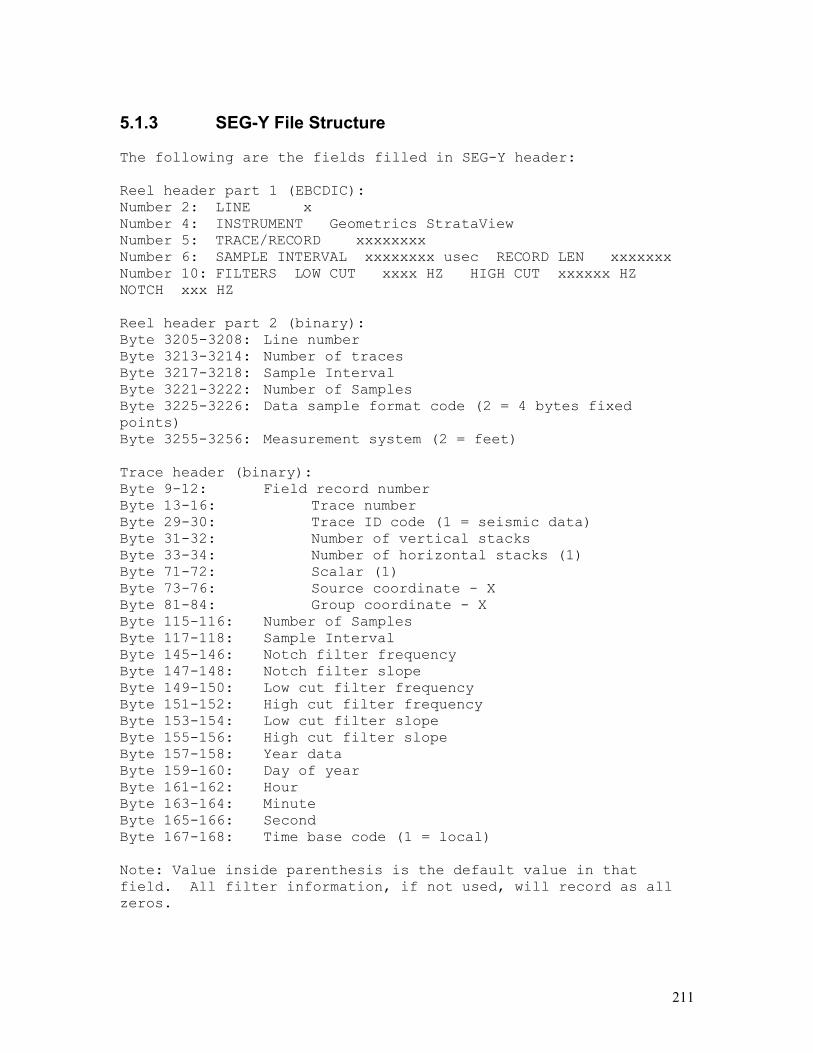
211
5.1.3 SEG-Y File Structure The following are the fields filled in SEG-Y header: Reel header part 1 (EBCDIC): Number 2: LINE x Number 4: INSTRUMENT Geometrics StrataView Number 5: TRACE/RECORD xxxxxxxx Number 6: SAMPLE INTERVAL xxxxxxxx usec RECORD LEN xxxxxxx Number 10: FILTERS LOW CUT xxxx HZ HIGH CUT xxxxxx HZ NOTCH xxx HZ Reel header part 2 (binary): Byte 3205-3208: Line number Byte 3213-3214: Number of traces Byte 3217-3218: Sample Interval Byte 3221-3222: Number of Samples Byte 3225-3226: Data sample format code (2 = 4 bytes fixed points) Byte 3255-3256: Measurement system (2 = feet) Trace header (binary): Byte 9-12: Field record number Byte 13-16: Trace number Byte 29-30: Trace ID code (1 = seismic data) Byte 31-32: Number of vertical stacks Byte 33-34: Number of horizontal stacks (1) Byte 71-72: Scalar (1) Byte 73-76: Source coordinate - X Byte 81-84: Group coordinate - X Byte 115-116: Number of Samples Byte 117-118: Sample Interval Byte 145-146: Notch filter frequency Byte 147-148: Notch filter slope Byte 149-150: Low cut filter frequency Byte 151-152: High cut filter frequency Byte 153-154: Low cut filter slope Byte 155-156: High cut filter slope Byte 157-158: Year data Byte 159-160: Day of year Byte 161-162: Hour Byte 163-164: Minute Byte 165-166: Second Byte 167-168: Time base code (1 = local) Note: Value inside parenthesis is the default value in that field. All filter information, if not used, will record as all zeros.

212
5.2 Storage Capacity The number of files which can be stored on a disk drive varies with the amount of disk or tape space required for a seismic record, which of course depends on the number of channels, data format, and record length. To calculate the number of bytes required, multiply the (number of channels used) * (record length in samples) * (number of bytes in a data word), then add some for the header information (approximately 700 bytes for the file header and Nx600 bytes for the trace headers). The amount of disk space or tape used depends on the record length as selected in the Acquisition Timing menu. The number of bytes in a data word is 4 (for 32-bit data storage format). The following table shows the number of files stored for different media for some combinations of channels, record length, and memory. These numbers are approximate. Warning. There are many combinations of record length which will not fit on a floppy disk. In some cases you can solve this problem by running a file compression program. In others, it will be necessary to write to an external SCSI device or to connect the seismograph to another computer through the RS-232 port and use a file transfer program such as Lap-Link. In general, the very long records will only be used with a vibrator source. Once the data is correlated, the resultant file will be much shorter.
Representative File Sizes No. of Record File Files/1.44 Files per Channels Length Size Mb Floppy Gigabyte (samples) 12 2048 106K 12 9400 12 4096 204K 7 4900 12 8192 394K 3 2500 12 16396 794K 1 1250 24 2048 212K 6 4700 24 4096 410K 3 2400 24 8192 800K 1 1250 48 2048 423K 3 2300 48 4096 816K 1 1200 48 8192 1600K 0 600 60 2048 528K 2 1900 60 4096 1020K 1 1000
213
5.3 Support Disks The StrataVisor and GeodeTM systems come with disks called "Support Disks" or in newer version, a support CD. These include programs and data used to support the system. The seismic program is included, along with sample data, and some additional files. The latest revisions to the software, format, and operating instructions will be found here. Geometrics has sample data sets for refraction and reflection surveys available on request. 5.3.1 Loading the seismic program The operating software of the Geode and StrataVisor is stored on hard disk drive C:. The software is normally resident in the system and will be loaded to configure the system as a seismograph. This software may also be loaded from drive A: or occasionally by CD in the case of a failure or, more commonly, to update the system software. To load the new software, simply insert the support disk and follow the instructions on screen.

214
6 Applications
6.1 Continuous Seismic Recording Using the Geometrics Geode
The Geode and NZ recording systems are capable of recording and transmitting data continuously. Data are broken up into contiguous records of user defined length. Settings can be adjusted so that there is overlap in the data, to facilitate recombination in processing. The minimum sample rate possible is a function of the number of channels in a single line, the length of the records that the data are cut into and highly dependent on the speed of the host computer. As a general rule, the faster, the better. For example, the following table shows possible sample interval and record length combinations using a 16 channel Geode and a 1.8 MHz P4 CPU. By using a combination less channels, a faster computer and/or multiple network cards, faster sample rates are possible Geode Minimum Cycle Times While in Continuous Mode Record Length (sec)-> 0.05 0.128 0.25 0.5 1 2Sample Rate (usec)
21 31.25
62.5 125 0.25 0.5 1.2 1.95250 0.3 0.5 1.2500 0.128
1000 n/a 2000 n/a
Numbers are approximate and are affected by the performance of the recording computer.
Continuous recording possible
Continuous recording not possible Occasional misses
Continuously recorded data can be time stamped either with the PC clock (accurate about a second per day) or the data can be synchronized using a pulse from a GPS fed to the trigger input.

215
6.1.1 Continuous Recording Using GPS Clock and Trigger
Timing Interface
In order to perform precisely timed continuous seismic recording using the standard Geometrics Geode or NZ system, the GPS Clock & Trigger Timing Interface Kit (P/N 28132-01) is offered. This kit consists of the following items: Geometrics P/N Qty Description 1 20-700-605 1 TRUETIME GPS-605 2 28148-01 1 CABLE ASSY, 12V POWER FOR GPS-605 3 28133-01 1 TRIGGER TIMING INTERFACE 4 28129-01 1 CABLE ASSY, 12V POWER FOR 28133-01 5 26960-01 1 CBL ASSY, TRIGGER (BNC TO 3-PIN) L 6 60-230-237 1 CABLE ASSY, 9-PIN D MALE/FEMALE 6FT 7 60-303-004 1 BNC CABLE M-M, 5FT POMONA 2249-C-60 8 28149-01 1 DOC, GPS TRIGGER TIMING INTERFACE
Item 1 above, the TrueTime GPS-605 receiver, consists of a clock with mounting bracket, an antenna, a 50ft antenna cable, and an operator’s manual. Check with the factory to discuss the use of other manufacturer’s GPS units. The item 8 document describes the several modes of operation of the timing interface. For the purpose of this paper, only the single controller, continuous mode is pertinent. In addition to the above, the standard Geode system is presumed to be available: Geode unit∗, battery, power cable, geophone sensors, analog spread cable, customized Ethernet cable, Ethernet cable adapter, and laptop PC with Ethernet adapter and Geometrics Seismic Controller Software (SCS) installed. The SCS requires registration with at least the following options enabled:
• External Alarm Box Support Enabled • Serial I/O Enabled • Continuous Recording Enabled • Trigger Window (recommended) • Subsample Trigger Synchronization Enabled/Disabled (as required by the application)
The last option allows disabling of the sampling resynchronization at the time of each trigger event. This may be desired to avoid the fractional sample interval time discontinuity which otherwise may occur at that moment. But it also limits the timing accuracy of the samples acquired after a trigger event to +/- 1 sample interval. See the Timing section below.
6.1.1.1 Hardware Setup The Geode, its battery, and the laptop PC are set up in the standard manner as explained in the Geode operator’s manual, with the exception of the trigger cable, as will be indicated below.
6.1.1.1.1 GPS: • Position the GPS antenna to allow good “visibility” of as large sky area as possible. This
generally means locating it above or away from nearby conductive materials or massive objects. To maintain constant lock on the GPS satellite signals, it must be able to receive good reception from at least three satellites at all times.
∗ A single Geode is assumed here for simplicity, however, the concepts (but not necessarily the performance) apply equally well to a multi-Geode system.

216
• Using the cable provided with this optional kit, connect the antenna to the GPS clock ANTENNA input.
• Use power cable 28148-01 to provide 12VDC power to the GPS clock unit, red clip to +12VDC and black clip to 12VDC return (-). The power source may be the same as that used for the Geode or a separate source. The display should immediately illuminate. After a few minutes, lock should be obtained, indicated by the suppression of the decimal point display segments.
• Use BNC cable 60-303-004 to connect the clock 1PPS output to the GPS Trigger Timing Interface "1PPS" input.
• Use the RJ11-to-DB9 adapter cable provided with the GPS clock to connect the clock RJ11 socket to the “GPS” DB9 connector on the GPS Trigger Timing Interface.
6.1.1.1.2 GPS Trigger Timing Interface • The Trigger Timing Interface is pre-set by the factory for a specified trigger cycle time,
based on the GPS 1PPS clock input.∗ If this should need to be changed, the unit must be opened by removing the two screws on the underside. A row of jumper selector pins, labeled LK1 through LK16, will be visible on the printed circuit board. LK1 through LK8 are involved in setting the cycle time. These eight positions constitute a binary weighted value, with LK1 being the least significant bit. The selected value plus one is the set cycle time. Thus, if no jumpers are inserted, a one-second cycle time would be selected; with a jumper only at LK1, a two-second cycle time would be selected; with a jumper only at LK2, a three-second cycle time would be selected. CAUTION: Do not alter the jumper selections on any other part of the printed circuit board.
• Use power cable 28129-01 to provide 12VDC power to the GPS clock unit, red clip to +12VDC and black clip to 12VDC return (-). The power source may be the same as that used for the Geode, the GPS, or a separate source.
• Use cable 26960-01 to connect the "TRIG 1" output to the Geode trigger input (hammer symbol), using an optional extension cable (P/N 23219-01) as required. (Note: the trigger output is an isolated open-drain FET that relies on the 3.3K-Ohm pull-up-to-5V resistor in the Geode trigger input circuitry.)
• Use serial cable 60-230-237 to connect the "CONTROLLER 1" DB9 connector to the laptop serial port.
6.1.1.2 Software Setup It is presumed here that the reader is already familiar with the customary operation of the Geode software, either from experience or from the operator’s manual supplied with the Geode. Only issues peculiar to the continuous recording application are addressed here. In order to setup the key software parameters correctly to achieve continuous recording, two requirements of the method should be understood:
∗ A modification of the Trigger Timing Interface has can be provided for custom applications, according to Customs and Specials Build Document #1008. Accordingly, a 16-position binary rotary switch has been added to the front panel and wired internally to selector pins in order to provide externally selectable trigger cycle times of 1, 3, 5, 7, 9, 11, … 27, 29, or 31 seconds.

217
1) The trigger delay should equal the negative of the record length. This condition means that the data record is ended by the trigger event, rather than the more usual case of being started by the trigger event. The importance of this is that the entire record is acquired and ready to be transmitted when the trigger event occurs.
2) The recorded data will be “continuous” (actually, sequential records will overlap) only if the achievable cycle time is less than the record length. In other words, if the actual cycle time is ever greater than the record length, then a gap in the data will result, making it discontinuous at that point. Achieving this requirement depends on a number of factors, some of which cannot be precisely controlled. Some of these factors are: the amount of data per record (which depends on the number of active recording channels and the sample rate), the data transmission speed to the laptop, the speed of the laptop PC, the writing speed to the hard drive, the tasks within the SCS that must occur for each record, and any other tasks that may be running which compete with the SCS for processor time.
A list of the important menu parameters follows. Some of these are directly affected by the two requirements given above. Acquisition menu Sample Interval Record Length Delay: (= -Record length) Stack Options: REPLACE ONLY Specify Channels: set to “DATA” those channels needed, others to “INACTIVE” File menu Storage Parameters Auto Save: checked Save to Disk: checked Display menu Trigger Parameters Cycle Time Scale: Cycle time of GPS Trigger Timing Interface, plus a fraction more System menu Trigger Options Holdoff 0.0s Arm Mode: Auto Sensitivity: near mid scale Alarms Setup Configure Alarm Box Serial Input Enabled: checked Geometrics Alarm Box Enabled: checked Baud Rate: 4800 Byte Size: 8 Parity Bit: None Stop Bits: 1 Stop Bit Terminator: LF Serial Input Setup - Replace PC time Stamp with GPS time: checked Advanced Acquisition Options Enable or Disable Subsample Trigger Synchronization: as required by application Enable Continuous Acquisition: checked When the recoding parameters and environment are selected for the first time, it is recommended that the actual cycle time be checked to ensure that requirement 2) is met. The Trigger Window

218
is most helpful for this purpose. Observe over the time span of a larger number of records whether or not the trigger cycle time exceeds the cycle time expected from the GPS Trigger Timing Interface. Be aware that PC interrupts can cause occasional triggering misses. If the observed performance is unacceptable, then adjustments must be made to increase the margin in order to maintain confidence in the capability of continuous recording with no gaps. Some of the obvious adjustments are:
• Reduce the number of recording channels by setting more of the highest numbered channels inactive.
• Increase the sample interval. • Reduce the record length (i.e., the overlap), but not such that it is less than or equal to the
desired cycle time (and remember to adjust the delay accordingly). • Use a faster PC and/or hard drive.
Some of the less obvious adjustments: • Reduce the relative overhead per record by increasing both the GPS Trigger Timer
Interface cycle time and the record length (and delay). • Reduce the workload created by unnecessary windows in the SCS. For example, reduce
the number of channels in the spectral window, if any. (Note that simply minimizing a window has little effect.) Registering the software without the extra windows (spectral, gather, etc.) is the best way.
• Minimize the background tasks running by uninstalling whatever software is not needed. The degree of margin can be ascertained by temporarily disconnecting the Geode trigger input and then setting the trigger sensitivity (under Trigger options in the System menu) to the maximum (100). In this mode the Geode will self-trigger as fast as possible and the margin relative to the desired cycle time can be observed in the Trigger window.
6.1.1.3 Timing The SCS log window normally records the time at which each file is saved, based on the PC clock. But with the “Serial Input Setup - Replace PC time Stamp with GPS time” checked in the Alarm Setup menu, the software will substitute the GPS serial time stamp as it is received. (Note that should there be a failure in the serial communication, the logged time will revert to PC time. Inspection of consecutively logged times can clear up any confusion since GPS time always shows exact second intervals.) The GPS time stamp indicates the time of the previous rising edge of the GPS 1PPS clock pulse, which is also the time at which the Geode is triggered.♣ Should the GPS lose lock on the satellites, it will continue issuing the 1PPS clock and the serial time stamp, but based on its own internal time base, which is subject to drift. Loss of lock is indicated by the illumination of all decimal points in the display, and by the “?” symbol appended to the end of the time stamp in the log file. With Subsample Trigger Synchronization (in System menu, Advanced Acquisition Options) disabled (i.e., no sample stretch at time of trigger), the last sample in a file record would represent
♣ From what has been described thus far, the GPS serial cable could be routed directly to the laptop PC, bypassing the GPS Trigger Timing Interface. However, the Interface serves two purposes, which may or may not be important for the application: to direct the time stamp to two PCs in the case of two controllers, and to receive the alarm information from the controller(s) over the same serial cable.

219
the time of the trigger edge +0/-1 sample interval. The first sample in the record would be similarly uncertain, plus any drift of the Geode 15ppm time base∗ over the time interval. With Subsample Trigger Synchronization enabled (i.e., possible sample stretch at time of trigger), the timing of all samples, after a trigger event until the next trigger event, can be known to +/- 1/32 of a sample interval#, plus any 15ppm drift. (But be aware that the overlapped portion of the record would be synchronized to a different GPS pulse, thus removing the accumulated drift at that point). Because the shot window display and the recorded file are based on the trigger that came after the data, they could indicate a one-sample error in timing. To recover the accurate time, one must find the location in the data file of the trigger that occurred near the beginning of the file (i.e., at the end of the previous file). This would be right after the data that overlaps the previous file. The overlapped portion is easy to identify because the data values recorded in that portion at the beginning of one file are identical to the values at the end of the previous file. Subsequent data in the file would be at a known time relative to that trigger (after applying the sample skew correction recorded in the SEG-2 file header) to within the accuracy stated. Also note that, because of the Geode time base drift relative to the GPS clock, the amount of overlap in a pair of sequential files can occasionally be one sample more or less than usual, depending on the direction of drift.
6.1.1.4 Alarm The alarm function of the GPS Trigger Timing Interface may or may not be important for a continuous recording application. It would be typically used for a remote monitoring situation in which it is critical that recording “down time” be minimized. Document 28149-01 describes the alarm functions in general. Here, a few comments will be made concerning the Alarm Setup menu in the SCS, which are particularly pertinent to continuous recording. The Alarm Setup menu is used to control which events produce which alarm indications with what tolerance. For example, the “Max Serial string not detected” entry may be used to alert the operator after a chosen number of serial time stamps from the GPS have been missed. Missed triggers resulting in data gaps may be monitored by using the “Max incomplete shot…” line. For no tolerance for this kind of failure, enter “1” in the first field and the expected cycle time in the second field. The next line, “Max consecutive incomplete shot”, may be used to allow isolated misses. For this, set up entries in the previous line, whether or not the alarm warnings are set to “OFF”. The “Alarm Idle. Reset Counter” button is used to clear the alarm state from the GPS Trigger Timer Interface, and to reset the event counters within the menu.
∗ Each channel within a Geode uses the same time base and so would experience the same drift. However, each Geode has its own time base so channels in different Geodes could experience different drifts. # At the higher sampling rates, the uncertainty increases somewhat, to about +/- 1/20 of a sample interval for the fastest sampling.

220
6.1.2 Continuous Recording Using The Internal PC Clock It is possible to continuously trigger the Geode or NZ seismograph without using the optional GPS and trigger timing interface kit. Geode/ES-3000 and NX seismographs are capable of triggering themselves, using the maximum trigger sensitivity settings under the system menu. When the Trigger Sensitivity slider is moved all the way to the right to the High sensitivity setting, the seismograph will continue to trigger repeatedly. Data records will be time stamped by the PC clock instead of the more accurate GPS clock.
6.1.2.1 Software Setup It is presumed here that the reader is already familiar with the customary operation of the Geode software, either from experience or from the operator’s manual supplied with the Geode. Only issues peculiar to the continuous recording application are addressed here. In order to setup the key software parameters correctly to achieve continuous recording, two requirements of the method should be understood:
1) The trigger delay should equal the negative of the record length. This condition means that the data record is ended by the trigger event, rather than the more usual case of being started by the trigger event. The importance of this is that the entire record is acquired and ready to be transmitted when the trigger event occurs.
2) The recorded data will be “continuous” (actually, sequential records will overlap) only if the achievable cycle time is less than the record length. In other words, if the actual cycle time is ever greater than the record length, then a gap in the data will result, making it discontinuous at that point. Achieving this requirement depends on a number of factors, some of which cannot be precisely controlled. Some of these factors are: the amount of data per record (which depends on the number of active recording channels and the sample rate), the data transmission speed to the laptop, the speed of the laptop PC, the writing speed to the hard drive, the tasks within the SCS that must occur for each record, and any other tasks that may be running which compete with the SCS for processor time.
A list of the important menu parameters follows. Some of these are directly affected by the two requirements given above. Acquisition menu Sample Interval Record Length

221
Delay: (= -Record length) Stack Options: REPLACE ONLY Specify Channels: set to “DATA” those channels needed, others to “INACTIVE” File menu Storage Parameters Auto Save: checked Save to Disk: checked Display menu Trigger Parameters Cycle Time Scale: Cycle time of GPS Trigger Timing Interface, plus a fraction more System menu Trigger Options Holdoff 0.0s Arm Mode: Auto Sensitivity: near mid scale Advanced Acquisition Options Enable or Disable Subsample Trigger Synchronization: as required by application Enable Continuous Acquisition: checked Calibration Mode Change calibration mode from every shot to many shots (99999) When the recoding parameters and environment are selected for the first time, it is recommended that the actual cycle time be checked to ensure that requirement 2) is met. The Trigger Window is most helpful for this purpose. Observe over the time span of a larger number of records whether or not the trigger cycle time exceeds the cycle time expected from the length of the records. Be aware that PC interrupts can cause occasional triggering misses. If the observed performance is unacceptable, then adjustments must be made to increase the margin in order to maintain confidence in the capability of continuous recording with no gaps. Some of the obvious adjustments are:
• Reduce the number of recording channels by setting more of the highest numbered channels inactive.
• Increase the sample interval. • Reduce the record length (i.e., the overlap), but not such that it is less than or
equal to the desired cycle time (and remember to adjust the delay accordingly). • Use a faster PC and/or hard drive.
Some of the less obvious adjustments: • Reduce the relative overhead per record by both increasing the record length and
decreasing the sample rate • Reduce the workload created by unnecessary windows in the SCS. For example,
reduce the number of channels in the spectral window, if any. (Note that simply minimizing a window has little effect.) Registering the software without the extra windows (spectral, gather, etc.) is the best way.
• Minimize the background tasks running by uninstalling whatever software is not needed.

222
6.2 Sub-Bottom Profiling Contact us at Geometrics for documentation discussing sub-bottom profiling
6.3 Surveillance ES-3000, Geodes and StrataVisor NZ seismographs can be configured to operate as surveillance monitors using the self-trigger algorithm. A warning box can be displayed upon detection, and the specific trigger channels are written into the log file to alert the operator that an event has been identified. To configure surveillance mode:
1. Turn on self-trigger mode in the Trigger Options dialog box.
2. Select whether you wish to use OR or AND channels for dectection. It is our experience that OR channels work best for local events like humans or animals walking. AND channels work best for distant events like trucks or aircraft. Note that the number of AND channels used to generate a trigger can be specified.
3. Set the length of the two adjacent detection windows w2 and w1 as well as the threshold. This will require some experimentation, depending on the event that you are trying to detect. It is best if you can simulate the situation in real life, and set these parameters accordingly. To detect a person walking in a noisy traffic area, we set time window w1 to 5 and time window w2 to 5 with a threshold ratio w2/w1 of 2. Window w1 measures background and w2 measures the event.
4. In the SYSTEMS>ALARMS SETUP dialog box, check the Report Self-Trigger alarm.
5. Set the acquisition parameters accordingly to define the record length and sample rate of the file that you would like to capture. This captured file can be used for more detailed data analysis, for example to determine the type of intruder or vehicle.
6. If you are not interested in saving records but only wish to use the self-trigger algorithm for detection:
a. Set the record length to a very small value b. Set the sample interval to the smallest value

223
c. Turn off Auto Save in the FILE menu d. Turn on Calibrate Every 99999 shots saved in the SYSTEM>Calibrate
mode dialog box. These changes will allow the system to recover very quickly so there is virtually no dead time in which an event might not be detected.
7. A detailed description of the operation of the self-trigger algorithm can be found in chapter 2.
Above is shown a screen capture of detected event. Note
• alarm box indicating the number of channels that detected the event • log file window showing channels that detected the event • noise monitor window showing real-time waterfall display of the event • spectral and shot windows recorded at higher sample rate for post-acquisition analysis
Shown opposite is the self-trigger dialog box settings used to detect the event shown above.

224
Appendix A. Specifications StrataVisor NZ and Geode Seismographs Configurations: 3, 6, 8, 12, 16 or 24 channels in weatherproof field deployable Geode module. Geode is operated from either 98/NT/2K/XP based laptop1 or by Geometrics’ ruggedized StrataVisor NZ field computer. Single Geodes are operated using SGOS software, which contains basic seismograph functions used for engineering surveys. Multiple Geodes can be connected together to build systems with many channels and many lines using MGOS software. A/D Conversion: 24 bit result using Crystal Semiconductor sigma-delta converters and Geometrics proprietary over sampling. Dynamic Range: 144 dB (system), 110 dB (instantaneous, measured) at 2 ms, 24 dB. Distortion: 0.0005% @ 2 ms, 1.75 to 208 Hz. Bandwidth: 1.75 Hz to 20 kHz. Low corner frequency option available. Common Mode Rejection: > 100dB at <= 100 Hz, 36 dB. Crosstalk: -125 dB at 23.5 Hz, 24 dB, 2 ms. Noise Floor: 0.20 uV, RFI at 2 ms, 36 dB, 1.75 to 208 Hz. Stacking Trigger Accuracy: 1/32 of sample interval. Maximum Input Signal: 2.8V PP at 0dB Input Impedance: 20 kOhm, 0.02 uf. Preamplifier Gains: Software selectable between 24 and 36 dB. Can be jumpered to allow selection of 12 or 24 dB or jumpered to 0 dB. Anti-alias Filters: -3 dB at 83% of Nyquist frequency, down 90 dB. Acquisition and Display Filters:
Low Cut: OUT, 10, 15, 25, 35, 50, 70, 100, 140, 200, 280, 400 Hz, 24 or 48 dB/octave, Butterworth. Notch: 50, 60, 150, 180 Hz and OUT, with the 50 dB rejection bandwidth 2% of center frequency. High Cut: OUT, 250, 500 or 1000 Hz, 24 or 48 dB/ octave.
Sample Interval: 0.02, 0.03125, 0.0625, 0.125, 0.25, 0.5, 1.0, 2.0, 4.0, 8.0, 16.0 ms. Correlation: Optional high-speed hardware correlator available in each Geode for fast cycle time with vibrators and pseudo-random (MiniSosie) sources2. Maximum Record Length: 16,384 samples per channel standard, 65,536 samples per channel optional. Pre-trigger Data: Up to 4,096 Samples. Delay: 0 to 9999 ms in 1 sample interval steps. Data Transmission: Uses reliable Ethernet connections and requires no custom transmission software. Interfaces directly with network capabilities of Windows 98/NT/2K/XP. Auxiliary Channels: All Geode channels can be programmed as either AUX or DATA. Fixed data and aux channels available in StrataVisor NZ. Roll Along: Built-in, no external roll box required. Line Testing: Real time noise monitor displays real-time output from geophones. Optional geophones pulse test helps identify bad geophones and shorted or broken cables2. Instrument Tests: Optional built-in daily, weekly and monthly testing available2. External laboratory quality test system available to measure noise, crosstalk, dynamic range, gain similarity and trigger accuracy to factory specification. Data Formats: SEG-2 standard with SGOS. SEG-D and SEG-Y available2. System Software:

225
Single Geode Operating Software (SGOS): Includes full compliment of acquisition, display, plotting, filtering and storage features. Multiple Geode Operating Software (MGOS): Allows single laptop to control multiple Geodes and adds additional preamp gains, correlation, expanded record length, tape writing, geophone pulse test, expanded test and diagnostics and roll along capability. StrataVisor NZ Software: Functionally similar to MGOS above but operates on ruggedized NZ field system. Data Storage: Stores data locally on laptop hard drive for transfer to portable media2. Plotters: Drives a variety of NT compatible printers including Printrex 4, 8 and 12 inch plotters. Consult factory. Triggering: Positive, negative or contact closure, software adjustable threshold. Power: Requires 12V external battery. Uses 0.65W/channel during acquisition, sleep mode reduces power consumption by 70% while in standby. Environmental: Geode:-30 to 70degrees C. Waterproof and submersible. Withstands a 1 m drop onto concrete on 6 sides and 8 corners. NZ: Starts from +5oC to 40oC. Operates from –5oC to 45oC. Physical: Geode: 12.2"L x 9 3/4"W x 7"D (31cmL x 24.75cmW x 17.75cm), weighs 3.5 kg. NZ field PC with no channels: 10.5“L x 18"W x 21“D (26.7cmL x 45.7 cmW x 53.34 cmD), weighs 30 lb (13.5 kg) Seismic recorder with 3-64 internal channels: 10.5“L x 18"W x 13 “D (26.7cm L x 45.7 cmW x 33 cmD), weighs 20 lb (9 kg) Operating System: Windows 98/NT/XP/2000. Data Processing and Interpretation: Includes refraction software with first break picking, layer assignment, depth below each geophone using delay time, refraction tomography and reflection processing software. Consult factory for individual data sheets. 1- Laptop computers are NOT field devices. They are easily damaged by harsh treatment or exposure to extreme environments. They have a short battery life. Geometrics StrataVisor NZ is designed to operate in harsh conditions for extended periods and should be used with the Geode for professional surveys when reliability is important.. 2 - Available with MGOS software only. ES-3000 Seismographs Configurations: 8 and 12 channels in weatherproof field deployable module. ES-3000 is operated from Windows 98/NT/2K/XP based laptop1 A/D Conversion: 24 bit result using Crystal Semiconductor sigma-delta converters and Geometrics proprietary over sampling. Dynamic Range: 144 dB (system), 110 dB (instantaneous, measured) at 2 ms, 24 dB. Distortion: 0.0005% @ 2 ms, 1.75 to 208 Hz. Bandwidth: 1.75 Hz to 8 kHz. Common Mode Rejection: > 100dB at <= 100 Hz, 36 dB. Crosstalk: -125 dB at 23.5 Hz, 24 dB, 2 ms. Noise Floor: 0.20 uV, RFI at 2 ms, 36 dB, 1.75 to 208 Hz. Stacking Trigger Accuracy: 1/32 of sample interval. Maximum Input Signal: 175 mV PP at 24dB Input Impedance: 20 kOhm, 0.02 uf. Preamplifier Gains: Software selectable between 24 and 36 dB. Anti-alias Filters: -3 dB at 83% of Nyquist frequency, down 90 dB. Acquisition and Display Filters:
Low Cut: OUT, 10, 15, 25, 35, 50, 70, 100, 140, 200, 280, 400 Hz, 24 or 48 dB/octave, Butterworth. Notch: 50, 60, 150, 180 Hz and OUT, with the 50 dB rejection bandwidth 2% of center frequency. High Cut: OUT, 250, 500 or 1000 Hz, 24 or 48 dB/ octave.

226
Sample Interval: 0.0625, 0.125, 0.25, 0.5, 1.0, 2.0 ms. Maximum Record Length: 4,096 samples per channel standard. Pre-trigger Data: Up to 4,096 Samples. Delay: 0 to 9999 ms in 1 sample interval steps. Data Transmission: Uses reliable Ethernet connections and requires no custom transmission software. Interfaces directly with network capabilities of Windows 98/NT/2K/XP. Auxiliary Channels: All ES-3000 channels can be programmed as either AUX or DATA. Fixed data and aux channels available in StrataVisor NZ. Data Formats: SEG-2 standard. System Software:
ES-3000 Operating Software (ESOS): Includes full compliment of acquisition, display, plotting, filtering and storage features.
Data Storage: Stores data locally on laptop hard drive for transfer to portable media2. Plotters: Drives a variety of NT compatible printers including Printrex 4, 8 and 12 inch plotters. Consult factory. Triggering: Positive, negative or contact closure, software adjustable threshold. Power: Requires 12V external battery. Uses 0.65W/channel during acquisition, sleep mode reduces power consumption by 70% while in standby. Environmental: ES-3000:-30 to 70 degrees C. Waterproof and submersible. Withstands a 1 m drop onto concrete on 6 sides and 8 corners. Physical: ES-3000: 12.2"L x 9 3/4"W x 7"D (31cmL x 24.75cmW x 17.75cm), weighs 3.5 kg. Operating System: Windows 98/NT/XP/2000. Data Processing and Interpretation: Includes refraction software with first break picking, layer assignment, depth below each geophone using delay time, refraction tomography and reflection processing software. Consult factory for individual data sheets. 1- Laptop computers are NOT field devices. They are easily damaged by harsh treatment or exposure to extreme environments. They have a short battery life. Geometrics StrataVisor NZ is designed to operate in harsh conditions for extended periods and should be used with the Geode for professional surveys when reliability is important.. 2 – Some additional features are available as options.

227
Appendix B. PCMCIA Card and Software Installation Installing your PCMCIA Card Geodes can be controlled either by the StrataVisor NZ or by a laptop or desktop computer. If you are using a laptop computer, the most common configuration is to install a PCMCIA card in the card bay found on the side. There are many variations in the PCMCIA cards that we have tried at Geometrics, and to date, have not found any network cards that do not work. However, you should try your card before going to the field to guard against incompatibilities.. Note that all systems purchased from us should have a PCMCIA card included. To install, follow the instructions that come with your PCMCIA card. Remember, SGOS and MGOS software work only under Windows ME, NT, 98 and 95. See our web site at www.geometrics.com for information on newer versions. Checking Your Network Settings These instructions may vary slightly with different versions of the Windows operating system. To check and see if your network card installed successfully, or to check if you have a network card already installed and the appropriate driver is operating, go to the Windows START button, select SETTINGS and choose CONTROL PANEL. In the CONTROL PANEL folder, select NETWORK and you will be presented with the menu opposite. If you select ADAPTERS, you should be shown a menu similar to one opposite, shown from the Windows NT operating system. Users of Windows 98 or Windows 95 will see something similar. This indicates that the network card has been installed properly and should be accessible from the Geode operating software. Installing Your Geode Software Geode Seismic Controller software (SCS) comes on floppy disks, CD ROM or can be downloaded from our web site. If the software does not automatically start, run the program SETUP and follow the instructions provided. Screens are self-explanatory, and if you make a wrong selection, you can press the BACK button to reverse any changes

228
Note: We strongly suggest that you exit all Windows programs before installing the software to avoid conflicts. The software will be installed in a default directory, unless you specify otherwise. . The installation is self-guiding, please follow the instructions on screen. Some menus require additional explanation. There are four installations options:
• Compact (smallest space possible)
• Custom (allows you to choose which options you require)
• Full installation (all tape support, 3rd party tools, recommended for most users)
• Full installation with no tape drive (does not install ASPI drivers for those systems for which there may be a system conflict with SCSI devices)

229
If you choose the CUSTOM installation, you will be presented with the following menu:
There are multiple options from which to choose:
• Seismodule Controller (basic operating software for the system). Always keep this option selected
• Tape Support (drivers for handling external SCSI tape devices) • Standard Filters (real time digital acquisition filters) • Test Box Script Files (needed if you own a Geometrics test system) • Survey Description Templates • Applications Sounds (WAV files for alerting operator of different acquisitions states) • Tools
o Tape and disk data reader (separate program) o Geode/NZ Bios Flash programmer (programs the firmware on the acquisition
boards o SEG2 to ASCII convert utility o SeisImager refraction processing package o SIPQC refraction package
You should leave all options checked unless you have a specific reason for removing them. Depending on your application, some parts of the M/SGOS operating software may not work properly, should you remove one. See sections in the Quick Start Guide and in Chapter One to connect your Geode/ES-3000 and laptop together and start the system.

230
Changing Imbedded Software Options After Installation If you have already installed the SCS software, you can make changes after installation via the SETTINGS>CONTROL PANEL>ADD/REMOVE PROGRAMS directly in Windows.
By clicking on the Change/Remove button, you are presented with the menu opposite:

231
By selecting the MODIFY button and clicking NEXT, you can review your installation instructions, shown in the opposite menu. Select or deselect the options that you require and press NEXT to modify your SCS software.

232
Appendix C: Sample Data Additional data sets are available on our downloads page at www.geometrics.com.

233
Appendix D: Applications software that ships with the Geode and StrataVisor NZ seismographs. This shipment contains industry-leading applications software to help you get the most from your new Geometrics Geode or StrataVisor seismograph. The applications software will help you analyze and process your data so you get answers quickly, for yourself and your clients. All software that can be launched from the seismograph program is preloaded on the StrataVisor seismograph, on a PC Geode controller (if purchased directly from Geometrics), and on your installation disks. If you are planning to use your own PC Geode controller, the software will be automatically loaded on your system when you install the Geode SGOS or MGOS operating program from the installation disks. There are two stand-alone packages, WinSeis Lite and WinSeis Turbo. These are reflection data processing packages and it is more practical to load them separately on the analysis PC where they will be used. All of the applications software packages are fully functional for analyzing your data, but usually limit the amount of data that can be analyzed. The full-featured packages are available either directly from Geometrics, Inc. or from the vendors listed below. The packages included with your Geode or StrataVisor are as follows.
• SIPQC refraction analysis software (delay-time method), from Rimrock Geophysics, P/N 26101-02. For support, please contact us, or Rimrock at [email protected] and 303-985-2522 (tel).
• SeisImager/2D refraction and modeling software (time-term inversion, delay-
time, and tomographic inversion methods), P/N 26112-01. For support, please contact us.
• WinSeis Lite reflection processing software (with Geode only) from the Kansas
Geological Survey (KGS), P/N 26100-08. For registration and support, please contact the KGS at [email protected] and 785-864-2176 (tel).
• WinSeis Turbo reflection processing software (with StrataVisor NZ only) from
the KGS, P/N 26100-03. For registration and support, please contact the KGS at [email protected] and 785-864-2176 (tel).
• Other experimental software may be on the system for your trial and assessment
The launchable software can be accessed from the ANSWERS menu, located on the main toolbar of the seismograph program. Some of the packages are best used with a mouse and keyboard connected; SeisImager/2D requires a mouse for operation. Support on all packages is available either from Geometrics or directly from the software vendor, as listed above, and support documentation is included with your shipment. We would be

234
pleased to help you interpret your first refraction data set to ensure that you understand the software and are able to use it to its fullest. Please contact the Geometrics Sales Department at 408-954-0522 (tel) or [email protected] to arrange an appointment. Real-time on-screen help is available through Microsoft NETMEETING over your high-speed Internet connection.