strandberg thesis 200419668/... · · 2006-03-30per erik strandberg lith - mai - ex - - 04 / 04...

Examensarbete

Mathematical models of bacteria population

growth in bioreactors: formulation, phase space

pictures, optimisation and control.

Per Erik Strandberg

LiTH - MAI - EX - - 04 / 04 - - SE

Mathematical models of bacteria population

growth in bioreactors: formulation, phase space

pictures, optimisation and control.

Applied Mathematics, Linkopings Univeritet

Per Erik Strandberg

LiTH - MAI - EX - - 04 / 04 - - SE

Examensarbete: 20 p

Level: D

Supervisor: Stefan Rauch,Applied Mathematics, Linkopings Universitet

Examiner: Stefan Rauch,Applied Mathematics, Linkopings Universitet

Linkoping: March 2004

Matematiska Institutionen581 83 LINKOPINGSWEDEN

march 2004

x

x

http://www.ep.liu.se/exjobb/mai/2004/tm/004/

LiTH - MAT - EX - - 04 / 04 - - SE

Mathematical models of bacteria population growth in bioreactors: for-mulation, phase space pictures, optimisation and control.

Per Erik Strandberg

There are many types of bioreactors used for producing bacteria pop-ulations in commercial, medical and research applications. This reportpresents a systematic discussion of some of the most important mod-els corresponding to the well known reproduction kinetics such as theMichaelis-Menten kinetics, competitive substrate inhibition and compet-itive product inhibition.We propose a modification of a known model, analyze it in the samemanner as known models and discuss the most popular types of biore-actors and ways of controlling them. This work summarises much of theknown results and may serve as an aid in attempts to design new models.

Chemostat, Continuous Stirred Tank Bioreactors (CSTR), DynamicalSystems, Mathematical Models in Biology, Biologic growth and Biologicproduction.

NyckelordKeyword

SammanfattningAbstract

ForfattareAuthor

TitelTitle

URL for elektronisk version

Serietitel och serienummer

Title of series, numbering

ISSN0348-2960

ISRN

ISBNSprakLanguage

Svenska/Swedish

Engelska/English

RapporttypReport category

Licentiatavhandling

Examensarbete

C-uppsats

D-uppsats

Ovrig rapport

Avdelning, InstitutionDivision, Department

DatumDate

Abstract

There are many types of bioreactors used for producing bacteria populationsin commercial, medical and research applications. This report presents asystematic discussion of some of the most important models corresponding tothe well known reproduction kinetics such as the Michaelis-Menten kinetics,competitive substrate inhibition and competitive product inhibition.

We propose a modification of a known model, analyze it in the samemanner as known models and discuss the most popular types of bioreactorsand ways of controlling them. This work summarises much of the knownresults and may serve as an aid in attempts to design new models.

Keywords: Chemostat, Continuous Stirred Tank Bioreactors (CSTR), Dy-namical Systems, Mathematical Models in Biology, Biologic growth andBiologic production.

Abstract in Swedish: Sammanfattning

Det finns manga typer av bioreaktorer som tillampas kommersiellt, och inommedicin och forskning. Denna rapport presenterar en systematisk redovis-ning av nagra av de viktigaste modellerna som motsvarar de kanda kinetiskaformerna Michaelis-Menten kinetik, kompetitiv substratinhibering och kom-petitiv produktinhibiering.

Vi foreslar en modifiering av en kand modell, analyserar den pa sammasatt som kanda modeller och redogor for de popularaste bioreaktortypernaoch hur de kan kontrolleras. Detta verk sammanfattar mycket av idag kandaresultat och kan anvandas som hjalp i design av nya modeller.

Strandberg, 2004. vii

Acknowledgements

I would like to thank my supervisor and examiner Stefan Rauch, at thedivision of applied mathematics for his excellent guidance, our rewardingdiscussions and his constant feedback.

I also have to thank Berkant Savas for helping to mature mathematically,for introducing me to the wonderful world of LATEX, and for his efforts inproofreading this material.

My opponent Andreas Andersson also deserves my thanks for his con-structive feedback and help in proofreading.

Strandberg, 2004. ix

Nomenclature

Most of the reoccurring abbreviations and symbols are described here.

Symbols

Y0 The amount of the variable Y inserted into a system.

Y The unit-dimension of the variable Y , for example t = 1s .Yi A steady state (number i) value of Y.

Ki Constants used in kinetic expressions, for example KI .

A The system matrix.a, b Growth- and non growth-associated production yield coefficients.c, ϕ, δ Fraction of X, F or S0. 0 < c < 1, 0 < ϕ < 1, 0 < δ < 1 .C, R The set of complex and real numbers.D Dilution coefficient; fraction of V replaced per timeunit.E Enzyme concentration in a system.F The flow of a media in or out of a system.P Product concentration in a system.S Substrate concentration in a system.V The volume of a system.X Biomass concentration in a system (kilogram/litre, etc.)X Vector containing S, X and P .

α1 Dimensionless maximal reproduction rate.α2 Dimensionless nutrition feed concentration.α, β Unitconsumtion of S needed to produce one unit of X or P .µ The general rate expression. µ = µ(S, X, P , . . . )

Strandberg, 2004. xi

xii

Abbreviations

CPI Competitive Product Inhibition (or Inhibited)CSI Competitive Substrate Inhibition (or Inhibited)CSTR Continuous Stirred Tank (bio)ReactorMMI Michaelis-Menten Inhibition (or Inhibited)

Contents

1 Introduction 1

1.1 Background . . . . . . . . . . . . . . . . . . . . . . . . . . . . 11.2 Problems we want to solve . . . . . . . . . . . . . . . . . . . . 21.3 Topics covered . . . . . . . . . . . . . . . . . . . . . . . . . . . 2

2 The ideal CSTR: the chemostat 5

2.1 Some simple models of biological growth . . . . . . . . . . . . 52.1.1 Exponential growth . . . . . . . . . . . . . . . . . . . . 52.1.2 The logistic equation . . . . . . . . . . . . . . . . . . . 52.1.3 A general batch reactor . . . . . . . . . . . . . . . . . . 7

2.2 The chemostat . . . . . . . . . . . . . . . . . . . . . . . . . . 72.2.1 The Continuous flow . . . . . . . . . . . . . . . . . . . 82.2.2 The Michaelis-Menten-kinetics . . . . . . . . . . . . . . 82.2.3 The dimensionless form of the chemostat . . . . . . . . 9

2.3 Analyzing the chemostat equations . . . . . . . . . . . . . . . 102.3.1 Equilibrium solutions of the chemostat . . . . . . . . . 102.3.2 Parameters α1 and α2 . . . . . . . . . . . . . . . . . . 112.3.3 Nullclines of the chemostat . . . . . . . . . . . . . . . 112.3.4 Linearization around the equilibrium points . . . . . . 122.3.5 The invariant line . . . . . . . . . . . . . . . . . . . . . 132.3.6 Looking at the phaseportrait . . . . . . . . . . . . . . . 142.3.7 Optimisation of the chemostat . . . . . . . . . . . . . . 152.3.8 Something about the products . . . . . . . . . . . . . . 16

3 A Chemostat with modified kinetics 19

3.1 The MMI-CSTR . . . . . . . . . . . . . . . . . . . . . . . . . 193.2 Invariant Line . . . . . . . . . . . . . . . . . . . . . . . . . . . 203.3 Nullclines . . . . . . . . . . . . . . . . . . . . . . . . . . . . . 203.4 Steady states . . . . . . . . . . . . . . . . . . . . . . . . . . . 203.5 Linearization around the equilibrium points . . . . . . . . . . 203.6 Looking at the phaseportrait . . . . . . . . . . . . . . . . . . . 22

Strandberg, 2004. xiii

xiv Contents

3.7 Optimisation . . . . . . . . . . . . . . . . . . . . . . . . . . . 223.8 From MMI-CSTR to chemostat . . . . . . . . . . . . . . . . . 233.9 Summary and comparison of the CSTRs . . . . . . . . . . . . 23

4 Other CSTR-types 27

4.1 Chemostats in series . . . . . . . . . . . . . . . . . . . . . . . 274.2 Chemostat with recirculation . . . . . . . . . . . . . . . . . . 284.3 Chemostat-like enzyme reactors . . . . . . . . . . . . . . . . . 29

5 Controlled CSTRs and the turbidostat 31

5.1 Controlled CSTRs . . . . . . . . . . . . . . . . . . . . . . . . 315.2 Invariant line for CSTRs controlled with D . . . . . . . . . . . 335.3 The turbidostat . . . . . . . . . . . . . . . . . . . . . . . . . . 335.4 The phaseportrait of a turbidostat . . . . . . . . . . . . . . . 35

6 Summary and conclusion 37

A The Linearized stability 41

A.1 The Linearization . . . . . . . . . . . . . . . . . . . . . . . . . 41A.2 The Stability . . . . . . . . . . . . . . . . . . . . . . . . . . . 41

B A Matlab M-file 43

Chapter 1

Introduction

This text is written as a master of science final thesis1 at the University ofLinkoping by Per Erik Strandberg with Stefan Rauch as supervisor and examiner,with Emacs in LATEX in 2003/2004.

This first chapter will define what is a Continuous stirred tank bioreactor anda chemostat. We give some background and formulate some main questions wewish to answer, and describe what topics are covered.

1.1 Background

Modeling of biological growth in reactors by dynamical systems started in the1950’s, when Monod, and Novick and Szilard developed the concept of Con-tinuous Stirred Tank (bio)Reactors(CSTRs) that differed from traditionalbatchreactors.

In a CSTR kinetics of the cellgrowth is sometimes referred to as a blackboxmodel , since all of the intra- and extra-cellular reactions are lumped intoone overall reaction. Typical equations describing blackbox models are verysimilar to enzymatic kinetics (where there is often one substrate and oneproduct in one reaction), such as the Michaelis-Menten kinetics used in theideal CSTR (the chemostat), often referred to as Monods model.

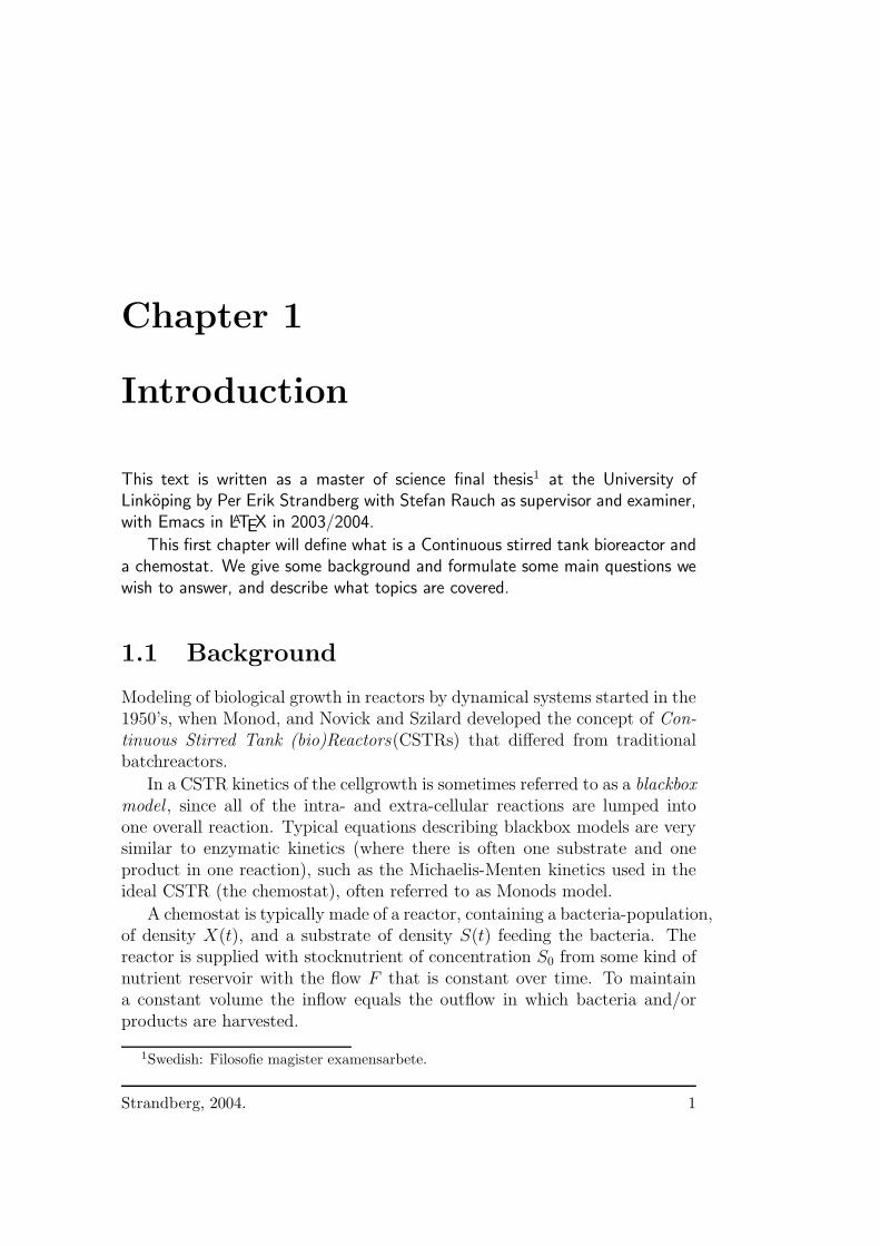
A chemostat is typically made of a reactor, containing a bacteria-population,of density X(t), and a substrate of density S(t) feeding the bacteria. Thereactor is supplied with stocknutrient of concentration S0 from some kind ofnutrient reservoir with the flow F that is constant over time. To maintaina constant volume the inflow equals the outflow in which bacteria and/orproducts are harvested.

1Swedish: Filosofie magister examensarbete.

Strandberg, 2004. 1

2 Chapter 1. Introduction

?

-X, S, µF , X, S

S0, F

Figure 1.1: The ideal CSTR: the chemostat, its inflow of nutrition, its growth(µ), and its outflow.

1.2 Problems we want to solve

This report provides a summary of already existing knowledge of bioreactorsand a detailed analysis of differential equations modelling bioreactors thatone usually encounters in textbooks. Some modifications of existing modelsare proposed and studied in detail.

This text aims to answer questions like “What types of bioreactors arethere?”, “If my bacteria population reproduces according to one of the kineticforms, how will it behave?”, “If my model is not really correct, how couldI change it?”, “What do I need to consider before fixing my model?”, andsome more.

1.3 Topics covered

There are five chapters (and this introduction) and two appendixes. Maintopics dealt with are:

Chapter 2: We explain the chemostat equations with the standard Michaelis-Menten kinetics by starting with two simple models of biological growth.We also present some tools useful for studying dynamical systems intwo dimensions.

Chapter 3: A new kinetic form is proposed and applied to an ideal CSTR.

Chapter 4: We leave the ideal CSTR and introduce, motivate and examinesome modified CSTRs.

Chapter 5: We look at controlled CSTRs.

Chapter 6: Summary and conclusion.

1.3. Topics covered 3

Appendix A: An appendix dealing with tools used to simplify the analysisof linearized stability in steady states.

Appendix B: A Matlab M-file is appended, showing how a program likeMatlab can be used to visualize and experiment with a given mathe-matical model.

4 Chapter 1. Introduction

Chapter 2

The ideal CSTR: the chemostat

In this chapter we study exponential growth, the logistic equation and thebatchreactors. We introduce the terminology, and explain how to think andhow to look at models and their describing differential equations.

We will derive and carefully analyze the chemostat equations. These equa-tions will constitute a reference model for the remaining parts of this text.

2.1 Some simple models of biological growth

2.1.1 Exponential growth

An extremely simple model could be dXdt

= µ·X where µ is the birth coefficientand X stands for bacteria density. If µ = constant > 0, we get X(t) = X0e

µt.

This is too simple a model. To limit the production of organisms we intro-duce a variable S describing concentration of the nutrient into the dynamicequations.

2.1.2 The logistic equation

Let us assume that dXdt

= µ·X, with µ = µ(S) = k ·S, and that dSdt

= −αkSX,meaning that each unit of bacteria density produces kS units of offspring pertime unit. With α = constant > 0 we could mean that each produced unitof offspring requires α units of nutrition. This model corresponds to ourintuition: the term SX says how often bacteria and food meet, giving thebacteria an opportunity to consume nutrient particles from the inflow S0 andto reproduce.

Strandberg, 2004. 5

6 Chapter 2. The ideal CSTR: the chemostat

We get a system of ordinary differential equations:

dXdt

= kSX (a)

dSdt

= −αkSX (b)

Multiplying (a) by α and adding (b) we get: ddt

(S + αX) = 0, thus (S +αX)(t) = S0 +αX0 = constant. In particular with t = 0 and X(0) = X0 ≈ 0(or at least small in comparison to a normal X(t)) we have S(0)+αX(0) ≈ S0,since X0 small implies S(t) = S0 − αX(t), giving us a reason to eliminate(b), and rewrite (a) as:

dX

dt= k(S0 − αX

︸︷︷︸

≈S(t)

)X = kS0︸︷︷︸

r>0

(1 −X

S0/α︸︷︷︸

B>0

)X = r(1 −X

B)X

By changing some factors we have reduced our system of ordinary differ-ential equations to a single equation, called the logistic equation:

dX

dt= r(1 −

X

B)X (2.1)

The factor r(1 − XB

), that corresponds to our old µ, is called an intrinsic1

growth-speed, and B the carrying capacity. By eliminating X instead of S,we quickly find dS

dt= −αr(1 − S

αB)S, an equation describing time change of

the nutrient concentration.When analyzing (2.1) we discover that for small values of X, when 0 < X ≪ B

we can approximate (2.1) by an exponential term and our model gives expo-nential growth for very small initial population densities.

The factor −XXB

in the equation corresponds to a crowding effect, inhibit-ing the reproduction rate.

The sign of (1 − XB

) is important to analyze. Let us assume that X ≥ 0.We also know that r > 0. Meaning that (1− X

B) is what determines the sign

of dXdt

.X = 0 ⇒ dX

dt= 0, a trivial solution, there is no population;

0 < X < B ⇒ (1 − XB

) > 0, the population grows;X = B ⇒ dX

dt= 0, constant population; and

X > B ⇒ dXdt

< 0, decreasing population.We now know that the model corresponds to our intuition. A small

population initially grows exponentially, later the term (1− XB

) starts to playrole. If ever X = B we will get a constant population. Finally: if X > B, N

1Swedish: “inre” or “inneboende”

2.2. The chemostat 7

will eventually diminish towards X = B. X = 0 and X = B are equilibriumsolutions, or steady states.

An explicit solution to (2.1) is: X(t) = X0BX0+(B−X0)e−rt , if 0 < X0 < B. It

can be found by separating variables in equation (2.1)

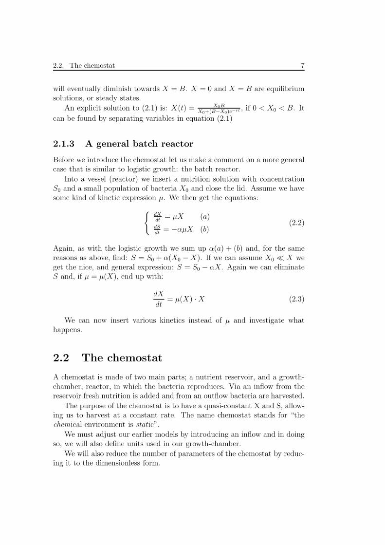
2.1.3 A general batch reactor

Before we introduce the chemostat let us make a comment on a more generalcase that is similar to logistic growth: the batch reactor.

Into a vessel (reactor) we insert a nutrition solution with concentrationS0 and a small population of bacteria X0 and close the lid. Assume we havesome kind of kinetic expression µ. We then get the equations:

dXdt

= µX (a)

dSdt

= −αµX (b)(2.2)

Again, as with the logistic growth we sum up α(a) + (b) and, for the samereasons as above, find: S = S0 + α(X0 − X). If we can assume X0 ≪ X weget the nice, and general expression: S = S0 − αX. Again we can eliminateS and, if µ = µ(X), end up with:

dX

dt= µ(X) · X (2.3)

We can now insert various kinetics instead of µ and investigate whathappens.

2.2 The chemostat

A chemostat is made of two main parts; a nutrient reservoir, and a growth-chamber, reactor, in which the bacteria reproduces. Via an inflow from thereservoir fresh nutrition is added and from an outflow bacteria are harvested.

The purpose of the chemostat is to have a quasi-constant X and S, allow-ing us to harvest at a constant rate. The name chemostat stands for “thechemical environment is stat ic”.

We must adjust our earlier models by introducing an inflow and in doingso, we will also define units used in our growth-chamber.

We will also reduce the number of parameters of the chemostat by reduc-ing it to the dimensionless form.


2.2.1 The Continuous flow

We let F = Fin = Fout having dimensions of volume/time. With Fin comesS0: “mass”/volume2. In the reactor we have a population of bacteria ofdensity X: mass/volume, and S: mass/volume.

We modify equation (2.1) by adding terms describing the inflow of thenutrition-solution and the outflow of bacteria, and assume µ = µ(S). Thus:

dXdt

= µ(S)X

new︷︸︸︷

−XF

VdSdt

= −αµ(S)X −SF

V+ S0

F

V︸︷︷︸

new

(2.4)

As we can see, F appears together with V in the form of F/V , so we setF/V = D - a dilution coefficient. It describes the fraction of volume beingreplaced in a unit of time.

The term X/V describes the density of bacteria, and by multiplying itwith F we get the amount of bacteria being flushed away in a unit of time.Similarly −DS corresponds to the outflow of the nutrient, and +DS0 to theinflow of the nutrient.

2.2.2 The Michaelis-Menten-kinetics

We will now discuss the reproduction coefficient, µ(S), by relating it to theMichaelis-Menten kinetics. This is the main “black box” we will see, and itis often also referred to as Monods kinetics.

Experimental data and similar cases in enzyme kinetics motivate the needof the reproduction-constant to be almost linear for small positive values for

S, but we also require an upper limit for µ so that: µ(S)S→∞−→ µmax. We

write down the Michaelis-Menten-kinetics:

µ(S) =µmaxS

KN + S

The new constant KN has an interesting meaning: KN

KN+KN= 1

2µmax. So

KN corresponds to the concentration at which µ = 12µmax

Let us see how µ(S) depends on S:Small S’s give us µ(S) ≈ S µmax

KN, if we can assume S ≪ KN , thus µ(S) is

almost linear. The maximum µ, µmax, is never reached, no matter how greatS gets, we have µ(S) < µmax.

2“Mass” could be moles, kilograms, molecules, etc.

2.2. The chemostat 9

The limit µ(S)S→∞−→ µmax is what we wanted. So µmax is the maximal

reproduction rate, achieved when the nutrient is unlimited.With this µ(S), the model becomes:

dXdt

= µmaxS

KN+SX − DX

dSdt

= −αµmaxS

KN+SX − DS + DS0

(2.5)

A more general CSTR, where Ω stands for other possible variables (X,(bi-) products, pH, . . . ) that may influence the reproduction rate, and X0

stands for bacteria density inserted via the in-flow, could be described by:

dXdt

= µ(S, Ω)X − DX + DX0

dSdt

= −αµ(S, Ω)X − DS + DS0

(2.6)

It is important to understand the structure of (2.6). We will look atothers CSTR’s, where this form is the common origin.

2.2.3 The dimensionless form of the chemostat

A quick glance at our equations show that we have a number of variableparameters: µmax, KN , D, α, and S0. Each one of them is important andnecessary, but is there a way for us to reduce the number of parameterssomehow? The answer is yes, and we will see that it is possible to eliminatethree of our constants (we eliminate five of them and introduce two new ones,this is possible since we have five parameters, and three dimensions).

As the title of this subsection suggests, we will actually eliminate thedimensions/units of the equations, but first we must investigate the units ofour constants. The first relation:

dim[dXdt

] = numbervolume·time

(here we assume dim[X] = number/volume and

dim[t] = time), thus: dim[µmaxXSKN+S

] = numbervolume·time

. With dim[S] = massvolume

weget dim[KN ] = mass

volumein order to keep KN + S meaningful, only allowing

dim[µmax] = 1time

.Our second relation: dim[dS

dt] = mass

volume·time, and since we know that

dim[S] = massvolume

, we get dim[S0] = massvolume

. So for α we get dim[α] =mass/volume

number/volume= 1.

And now, to simplify, we replace S, X, and t with S · S, X · X, and t · t.Where S, X and t corresponds to the unit-dimension, whatever they maybe.3 Our elegant equation (2.5) will now for a moment be replaced with:

3Note that t could be a second, a year, 3.25489677 minutes, etc, X could be onebacteria, twelve bacterias or 2.553 kg of dry cellweight per litre, gallon or tankvolume,and S could typically be: mol/l, molecules/mm3 or 3.333 lb/gallon.


dXdt

· Xt

= µmaxSS

KN+SSXX − DXX

dSdt

· St

= −αµmaxSS

KN+SSXX − DSS + DS0

Now, to get a dimensionless form, we multiply the dX-row with t/X, and

the dS-row with t/S, allowing us to fix t = 1D

, S = KN , X = Sαµmax t

=KNDαµmax

, and replace α1 = tµmax = 1D

µmax and α2 = S0

S= S0

KN= tDS0

S. These

replacings give:

dXdt

= α1S

1+SX − X

dSdt

= − S1+S

X − S + α2

(2.7)

Showing that the chemostat effectively depends on two parameters α1 andα2.

2.3 Analyzing the chemostat equations

For the chemostat equations we find equilibrium solutions, null-clines, in-vestigate interesting values of the parameters α1 and α2, linearize equations(2.7) around equilibrium points and find an invariant line.

2.3.1 Equilibrium solutions of the chemostat

To find equilibrium solutions we solve:

dXdt

= α1(S

1+S)X − X = 0

dSdt

= −( S1+S

)X − S + α2 = 0⇒

0 = α1(

S1+S

)X − X

0 = −( S1+S

)X − S + α2

One trivial solution is X = 0. Inserting this into the second relation givesus S = α2 thus one equilibrium solution is: (X0, S0) = (0, α2). This is ourfirst hint indicating that α2 has a meaning of a dimensionless stock-nutrient-concentration.

The other (non-trivial) solution is more interesting. We get: X = α1(S

1+S)X

and for X 6= 0, S = 1α1−1

.

Combining this with the second equation, we get: X = α1(α2−1

α1−1). So

we have two equilibrium points:

(X0, S0) = (0, α2)

(X1, S1) =(

α1(α2 −1

α1−1), 1

α1−1

)(2.8)

2.3. Analyzing the chemostat equations 11

2.3.2 Parameters α1 and α2

Let us discuss when α1 and α2 give us an equilibrium having biological mean-ing.

We saw that α1 = µmax

D. Giving us the hint that α1 could be interpreted

as a kind of dimensionless reproduction-rate, or even more interestingly: as amaximum reproduction-rate multiplied by the inverse of the flushing factor.

Combining our intuition with the solutions we found above, we notice:S1 = 1

α1−1, this must be positive for the population to exist, giving us: α1 > 1.

Meaning that we must limit the dilution rate to be smaller than the maximalreproduction rate.

From the trivial solution we notice that S0 = α2 = S0

KNcharacterises

nutrient. But as we will see, this is one way of dealing with α2. Anotherway of looking at this parameter is to interpret it as an inverse number ofKN , or as the amount of S we have, measured in units of KN . We saw thata small KN means that we are closer to µmax for lower values of S. So smallKN means that α2 is large and vice versa.

Looking at our non-trivial solution again we notice that X1 = α2 −1

α1−1

must be positive for the population to exist. Requiring α2 > 1α1−1

. (Thusα2 > 0.) Here we can see that for small (α1 − 1) (large flushing or weakreproduction) we need α2 to be large (strong flushing or weak reproduction,requires more food in order to reproduce faster), and a large α1 allows α2 tobe small. This is how the model tells us that if it easy to reproduce we havea lower need of nutrition.

2.3.3 Nullclines of the chemostat

A useful tool for investigating this kind of dynamic systems are nullclines,the lines where dX

dt= 0, or dS

dt= 0. We also understand that at the crossing

of two different kind of nullclines there is an equilibrium point.Let us begin with the X-relation: 0 = dX

dt= α1(

S1+S

)X−X, we notice that

one nullcline is: X = 0, and the other ones is: α1(S

1+S) − 1 = 0 so S = 1

α1−1.

Continuing with the nullclines for S: 0 = dSdt

= −( S1+S

)X − S + α2 = 0,

after some elementary work, we get: X = (α2−S)(1+S)S

. Our nullclines aregiven by:

X = 0 ⇒ X = 0 or S = 1α1−1

S = 0 ⇒ X = (α2−S)(1+S)S

The nullclines are easy to draw, and by drawing some vectors in the firstquadrant, we can get a pretty good idea of how a state (X(t), S(t)) moves


around in the (X,S)-plane over time.

2.3.4 Linearization around the equilibrium points

We have found two equilibrium solutions in the positive quadrant of the

(X,S)-plane: (X0, S0) = (0, α2) and (X1, S1) =(

α1(α2 −1

α1−1), 1

α1−1

)

. We

want to study in the neighbourhood of these points how the chemostat re-sponds to small disturbances. Does it wander away from an equilibrium ordoes it fall back onto it? The question we want to answer is: is the solutionstable?

In order to analyze the chemostat’s behaviour at the equilibrium we willuse the stability conditions described in Appendix A. The stability conditionsare tr(A) < 0 and det(A) > 0. For eigenvalues of the linearization matrix A

to be real we need −4 det(A) + tr(A)2 > 0.

We find (see Appendix A):

A =

(a11 a12

a21 a22

)

=

(

α1S

1+S− 1 α1X

(1+S)2

− S1+S

− X(1+S)2

− 1

)

Evaluating this at the trivial equilibrium point (X0, S0) = (0, α2) we get:

A =

( α1α2

1+α2− 1 0

− α2

1+α2−1

)

⇒

tr(A) = α1α2

1+α2− 2

det(A) = − α1α2

1+α2+ 1

We know that we have two conditions for stability around an equilibriumpoint: tr(A) < 0 and det(A) > 0. We will notice that our second condition:− α1α2

1+α2+ 1 > 0 ⇔ 1 > α1α2

1+α2is in conflict with the earlier condition for

physical meaning, α2 > 1α1−1

⇔ 1 < α1α2

1+α2. So this steady state is not

stable.

At the other equilibrium point, (X1, S1) =(

α1(α2 − 1α1−1

), 1α1−1

)

, by

renaming the term X1

(S1+1)2 = σ and remember that σ > 0, we get:

A =

(0 σα1

− 1α1

−σ − 1

)

⇒

tr(A) = −σ − 1 < 0.det(A) = σ > 0.

The non-trivial equilibrium point is thus stable. We also note that:−4 det(A) + tr(A)2 = −4σ + σ2 + 2σ + 1 = σ2 − 2σ + 1 = (σ − 1)2 > 0. Sotrajectories of a state near this point are not spiraling since their eigenvectorsare real. They go more straight-forward towards (X1, S1).


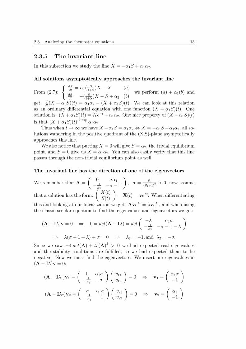
2.3.5 The invariant line

In this subsection we study the line X = −α1S + α1α2.

All solutions asymptotically approaches the invariant line

From (2.7):

dXdt

= α1(S

1+S)X − X (a)

dSdt

= −( S1+S

)X − S + α2 (b)we perform (a) + α1(b) and

get: ddt

(X + α1S)(t) = α1α2 − (X + α1S)(t). We can look at this relationas an ordinary differential equation with one function (X + α1S)(t). Onesolution is: (X +α1S)(t) = Ke−t +α1α2. One nice property of (X +α1S)(t)

is that (X + α1S)(t)t→∞−→ α1α2.

Thus when t → ∞ we have X −α1S = α1α2 ⇔ X = −α1S +α1α2, all so-lutions wandering in the positive quadrant of the (X,S)-plane asymptoticallyapproaches this line.

We also notice that putting X = 0 will give S = α2, the trivial equilibriumpoint, and S = 0 give us X = α1α2. You can also easily verify that this linepasses through the non-trivial equilibrium point as well.

The invariant line has the direction of one of the eigenvectors

We remember that A =

(0 σα1

− 1α1

−σ − 1

)

, σ = X1

(S1+1)2 > 0, now assume

that a solution has the form:

(X(t)S(t)

)

= X(t) = veλt. When differentiating

this and looking at our linearization we get: Aveλt = λveλt, and when usingthe classic secular equation to find the eigenvalues and eigenvectors we get:

(A− Iλ)v = 0 ⇒ 0 = det(A − Iλ) = det

(−λ α1σ− 1

α1−σ − 1 − λ

)

⇒ λ(σ + 1 + λ) + σ = 0 ⇒ λ1 = −1, and λ2 = −σ.

Since we saw −4 det(A) + tr(A)2 > 0 we had expected real eigenvaluesand the stability conditions are fulfilled, so we had expected them to benegative. Now we must find the eigenvectors. We insert our eigenvalues in(A − Iλ)v = 0:

(A − Iλ1)v1 =

(1 α1σ

− 1α1

−σ

)(v11

v12

)

= 0 ⇒ v1 =

(α1σ−1

)

(A − Iλ2)v2 =

(σ α1σ

− 1α1

−1

)(v21

v22

)

= 0 ⇒ v2 =

(α1

−1

)


By elongating the eigenvector v2 in positive and negative directions from(X1, S1) we can easily verify that this is the same line as X = −α1S + α1α2.Thus a state starting on the invariant line can not move away from it.

An observation

By the theorem of existence and uniqueness of solutions of ordinary differ-ential equations two trajectories cannot cross each other. Thus the invariantline (consisting of trajectories) cannot be crossed. This helps in understand-ing how trajectories behave in the neighbourhood of the invariant line (seefigure 2.1).

The invariant line: conclusions

We can now conclude that the invariance line can be seen as a barrier for thesolutions. No solution above it can get below it and vice versa. This gives us aguidance in drawing a phase portrait, and we can see in the Matlab simulationthat, indeed, the solutions near the non-trivial equilibrium solution can notmove around in spirals.

2.3.6 Looking at the phaseportrait

When looking at the phaseportrait we will plot trajectories using Eulersmethod: Xn+1 = Xn + ∆t · d

dtXn. We can call this kind of trajectory an

Euler path.

The phaseportrait of this kind of a system gives us a lot of information.In this example we can see the invariant line (dotted), the nullclines, andan Euler path (point-dotted) starting at a low amounts of both bacteria andnutrition rates. In this example we understand that the state at first wanderstowards higher amounts of nutrition (the bacteria are slowly reproducing).When there is sufficient amounts of nutrition the state wanders off towardsmore bacteria slowing the increase of nutrition, bending it off to the rightthen getting almost parallel to the invariant line, and finally asymptoticallyreaching the steady state.

In figure 2.1 (and the following figures in later sections) we can see α2

where the invariant line crosses the S-axis (in the trivial steady state thereare no bacteria and stock-concentration of nutrient). We can also find α1α2

at the invariant lines crossing of the X-axis. From this information we canfind the dimensionless units of X and S if we would like.


0 1 2 3 4 5 6 7 8 90

0.5

1

1.5

2

2.5

3

3.5

4

4.5

X

S

Figure 2.1: A phaseportrait of a chemostat. The dotted line is the invariantline, the point-dotted line an Euler path and the Continuous lines are null-clines (the S-axis is an X-nullcline). The arrows represent the vector-field(dX

dt, dS

dt). Notice that the Euler path approaches the invariant line but never

crosses it.

2.3.7 Optimisation of the chemostat

Now we will leave the dimensionless form and return to the general model,(2.6). We will adapt it to fit the chemostat, and express the steady statesin a different way. We will do so since many of the parameters we changedin finding the dimensionless form includes the dilution coefficient D, and weneed to compute d

dD(DX) in order to find an optimal value for D. The model

is now: dXdt

= µX − DXdSdt

= −αµX − DS + DS0

If we focus on the nontrivial steady state (ignoring the indexes): (X, S), wefind D = µ if we let dX

dt= 0, simplifying the relationdS

dt= 0 = −αDX −

DS + DS0 ⇔ X = 1α(S0 − S).

For Monods kinetic expression, we let D = µ = µmaxS

KS+S⇔ S =

DKS

µmax−D, and now we can find an expression for X: X = 1

α(S0 −

DKS

µmax−D).

We are easily convinced that this expression multiplied with D is one wayto measure the amount of productivity, if we assume that productivity isgrowth-associated, or if we are interested in the bacteria in itself (as in theyeast-production).

Now we have Xout = XD and we want to maximize this, and find an

optimum. We calculate ddD

(XD) and find D = µmax(1 ±√

KS

S0+KS), but (as


we saw earlier) D = µ, so there is no way D could be greater than µmax,

leaving us with the only possible solution: Dmax = µmax(1−√

KS

S0+KS) ⇒

Xout,max = 1α

(

S0 + KS −√

KS(S0 + KS))

.

2.3.8 Something about the products

So far, we have only considered a system where biomass and substrate con-centration were described. Biomass, as for yeast production is usually thevariable of interest. Sometimes, as for waste treatment, the substrate is whatis interesting. But there is also the possibility that another variable P , theproduct, is what we want to know more about.

A common way to describe the change in product density is to assumethat there are both growth- and non-growth-associated production. Thegrowth-associated production is proportional to the ammount of growth bythe constant a, and the non-growth-associated production to the bacteriadensity by the constant b. We get the us the system:

dXdt

= µX − DX

dSdt

= D(S0 − S) − αµX − β(aµX + bX)

dPdt

= aµX + bX − DP

(2.9)

We recognize α as the unit-consumption of S required to produce one unit ofX, and β as the unit-consumption of S required to produce one unit of P The“new” constants a and b describe the difference between growth-associatedproduction and non-growth-associated production respectively.

Looking for a nontrivial steady state we let dXdt

= 0 and find µ = D, fromthis we can usually find S if we have X, and P . P is found by taking µ = Dand dP

dt= 0 ⇒ P = aX + bX

D. Finding X requires a little work, and

we calculate: dSdt

= 0 ⇔ X(αD + βaD + βb) = D(S0 − S) ⇔ X =S0−S

α+β(a+ bD

), so the (non-trivial) steady state for a general µ is:

X = S0−Sα+β(a+ b

D)

P = aX + bXD

µ = D ⇒ S

If we are interested in S we can often easily find it from the above relations.If we use the only kinetics we have encountered so far, the Monod kinetics,we again find: S = DKS

µmax−Dand get:


S = DKS

µmax−D

X = S0−Sα+β(a+ b

D)

P = aX + bXD

As in Optimising Xout the Optimisation of P requires computing d(DP )dt

= 0.

Chapter 3

A Chemostat with modified

kinetics

We have considered so far a chemostat with Monods kinetics. In this chapter wewill investigate our modification of this model.

Similarities with Monods equations will aid us in performing an analysis ofthe equations in a similar way as in Chapter 2.

3.1 The MMI-CSTR

We call this model the Michaelis-Menten inhibited Continuous stirred tankreactor (MMI-CSTR) since we use a kind of Michaelis-Menten kinetics tolower the influence of growing values of X in the kinetic expression. We takethe term µ = µmax

SKS+S

XKX+X

in our equations instead of µmaxS

KS+SX, as in

Monods chemostat. This kinetic form describes the situation when a highdensity, X, of bacteria inhibits the growth in the chemostat.

By introducing the proposed inhibition we get the MMI-CSTR:

dXdt

= µmaxS

KS+SX

KX+X− XD

dSdt

= −αµmaxS

KS+SX

KX+X− SD + S0D

(3.1)

To obtain a nondimensional form we replace S, X and t with S · S, X · Xand t · t. We start by multiplying the relations with t/X and t/S respectively

then replace t = 1D

, S = KS, X = Sα µmax

KXt, and replace α1 = µmax

KXDand

α2 = S0

S. Finally, we let KX = XCX, to write the equations as:

Strandberg, 2004. 19

20 Chapter 3. A Chemostat with modified kinetics

dXdt

= α1S

1+SX

1+ XXC

− X

dSdt

= − S1+S

X1+ X

XC

− S + α2

(3.2)

3.2 Invariant Line

As previously, we can find that X = α1(α2 − S) in an invariant line.

3.3 Nullclines

We let dXdt

= 0 and find the line X = 0, but also S =1+ X

XC

α1−(1+ XXC

). Now, if

dSdt

= 0 we get: X = (α2−S)(1+S)

S+ 1XC

(α2−S)(1+S). So the nullclines are:

dXdt

= 0 ⇒ X = 0 or S =1+ X

XC

α1−(1+ XXC

)

dSdt

= 0 ⇒ X = (α2−S)(1+S)

S+ 1XC

(α2−S)(1+S)

3.4 Steady states

Using the first of the dXdt

= 0 nullclines we find the same trivial steady state:(X0, S0) = (0, α2). If we use the second relation in combination with theinvariant line to eliminate X we end up with the second degree equation:

S2 + S (XC + 1 −XC

α1− α2)

︸︷︷︸

p−q

+ (−XC

α1− α2)

︸︷︷︸

−q

= 0, with the solutions

S = q−p2

±√

( q−p2

)2 + q. One can quickly find that the solution with a minus

is negative, so we reject it. The other solution however must be smallerthan α2 in order for the X associated to it to be positive, so the following

assumptions are needed: α2 > −p−q2

+√

(p−q2

)2 + q ⇔ α2 > 1α1−1

, for

any non-trivial steady state to exist. We also understand that α1 > 1. Theseconditions will be used later.

3.5 Linearization around the equilibrium points

For the MMI-CSTR the system matrix A is:

3.6. Looking at the phaseportrait 21

A =

α1S

1+S1

(1+ XXC

)2− 1 α1

1(1+S)2

X1+ X

XC

− S1+S

1(1+ X

XC)2

− 1(1+S)2

X1+ X

XC

− 1

.

When we investigate the trace and the determinant at the steady stateswe may use the relation: dX

dt= 0 ⇔ α1XS = X(1 + S)(1 + X

XC), to

simplify the matrix A (for X 6= 0):

A =

11+ X

XC

− 1 XS(1+S)

−1/α1

1+ XXC

−X/α1

S(1+S)− 1

=

−X

XC

1+ XXC

XS(1+S)

−1/α1

1+ XXC

−X/α1

S(1+S)− 1

.

As we can see: trA < 0, but how about det(A), is it positive? Weeliminate some of our X by using the invariant line:

A =

− XXC

1+ XXC

α1(α2−S)S(1+S)

−1/α1

1+ XXC

−(α2−S)S(1+S)

− 1

⇒

det(A) =X

XC

1 + XXC

( α2 − S

S(1 + S)+ 1)

+α2 − S

(1 + XXC

)(1 + S)> 0

Thus, the nontrivial steady state is stable.

If we now study the trivial steady state, we have X = 0, so A is:

A =

(α1α2

1+α2− 1 0

− α2

1+α2−1

)

⇒

tr(A) = α1α2

1+α2− 2 ⇒ α1α2

1+α2< 2, for stability.

det(A) = −( α1α2

1+α2− 1) ⇒ α1α2

1+α2< 1, for stability.

So, we have to have α1α2

1+α2< 1 ⇔ α2 > 1

α1−1to have a stable trivial

steady state, but we remember the constraint for the non-trivial steady stateto exist: α2 < 1

α1−1, we can conclude that if we flush too much; no population

will exist, like expected.


0 2 4 6 8 10 12 14 16 180

0.5

1

1.5

2

2.5

3

3.5

X

S

Figure 3.1: Phaseportrait of the MMI-CSTR.

3.6 Looking at the phaseportrait

Again, in figure 3.1, we have α1α2 where the invariant line crosses the X-axis,and α2 where it crosses the S-axis. We see that the nullclines have similarpositions in the phaseplane and that the Euler path has a similar behaviour.This phase-portrait is very similar to the chemostat one. But we notice thatindeed the MMI-CSTR responds to large values of X by inhibition.

3.7 Optimisation

From the general model (2.6) we quickly get: µ = D and X = 1α(S0S)

if we ignore the trivial steady state and drop the indices. From µ = Dwe can find X in order to eliminate it: X = µmax

SS

KS+S− KX = 1

α(S0 −

S). This expression give rise to the same kind of second degree equation

as earlier: S2 + S (αµmax

D+ KS − αKS − S0)

︸︷︷︸2wD

+2λ

+ KS(−αKX − S0)︸︷︷︸

−v

= 0. This

equation gives us an S with dimensions. We can use this dimensional S to

find DX: DX = S0 + wα

+ Dλα

−

√

(wα

+ Dλα

)2 + D2vα2 .

This can be differentiated in order to find ddD

(DX) = 0.

3.8. From MMI-CSTR to chemostat 23

3.8 From MMI-CSTR to chemostat

A quick comparison of the dimensionless µ’s of the chemostat and the MMI-CSTR reveals that the new term 1

1+ XXC

inhibits both dXdt

and dSdt

. This inhibi-

tion is stronger the smaller XC is. Thus in the limit of XC → ∞ we recover:

µMMI = α1S

S+11

1+ XXC

XC→∞−→ α1

SS+1

= µchemostat.

3.9 Summary and comparison of the CSTRs

We have discussed two different chemostatmodels with two different kineticforms: Monods Kinetics and the Michaelis-Menten Inhibited kinetics. Twoother well studied kinetics are Competitive Substrate Inhibition (where thedimensionless µ = S

1+S+ S2

KI

) and Competitive Product Inhibition (µ = S1+S+KIX

)

that we call CSI-CSTR and CPI-CSTR.

In the table below there is a summary of the models (we have excludedthe trivial X-nullcline X = 0 and abbreviated nullcline ‘XNC’ and ‘SNC’ forX-nullcline and S-nullcline).

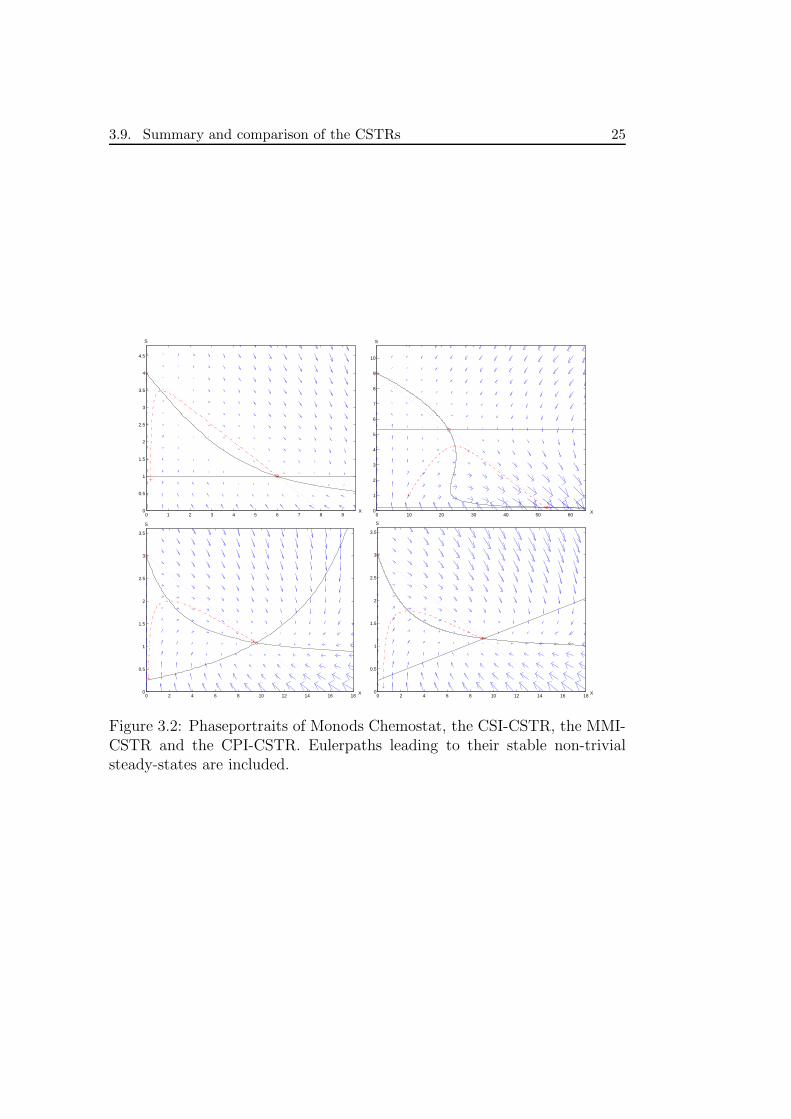
By comparing the phaseportraits (figure 3.2) it is easy to see obvioussimilarities in all models. Some common features are the existence of theinvariant line and the equilibrium points. The invariant line exist due tothe fact that the model produces a constant value of bacteria density perconsumed unit of substrate density. The equilibrium points vary with theparameters α1, α2 and various constants. By choosing them carefully we maydetermine the position of the equilibrium points in the phase-plane, or wecan force the model to flush the bacteria population out of the chemostat.

Looking at the CSI-CSTR one can see that the steady state value for Sis relatively low (compared to the other models), one can reason that thisis due to the response of this model to inhibition of S. In this model wecan also see that the points on the Euler path never reach large values ofS (relative to the other models), this must a problem for real CSI-CSTRs:starting such a reactor must be done carefully. Another feature of this modelis that the vectorfield is not “clockwise” around the non-trivial steady state.Instead it seems to rapidly push a state towards the unstable steady state(for small or large values of both S and X) and close to the invariant linesit pushes the state towards the trivial or non-trivial steady state.


Model Monods Chemostat CSI-CSTR

µ S1+S

S

1+S+ S2

KI

dXdt

α1S

1+SX − X α1

S

1+S+ S2

KI

X − X

dSdt

− S1+S

X − S + α2 − S

1+S+ S2

KI

X − S + α2

XNC S = 1α1−1

S = KI(α1−1)2

±

√

(KI(α1−1)2

)2− KI

SNC X = (α2−S)(1+S)S

X =(α2−S)(1+S+ S2

KI)

S

limit − KI → ∞

Model MMI-CSTR CPI-CSTR

µ S1+S

11+ X

XC

S1+S+KIX

dXdt

α1S

1+SX

1+ XXC

− X α1S

1+S+KIXX − X

dSdt

− S1+S

X1+ X

XC

− S + α2 − S1+S+KIX

X − S + α2

XNC S =1+ X

XC

α1−(1+ XXC

)S = XKI+1

α1−1

SNC X = (α2−S)(1+S)

S+ 1XC

(α2−S)(1+S)X = (α2−S)(1+S)

S−KI(α2−S)

limit XC → ∞ KI → 0

The other three models, the chemostat, the MMI-CSTR and the CPI-CSTR are quite similar in comparison to the CSI-CSTR. They have thesimilar nullclines and steady states in almost the same places and their vec-torfields are also similar. The chemostat S-nullcline is parallel to the X-axisand in two other models this nullcline increases with increasing values of X.This can be interpreted as an inhibiting effect of X on µ: the vectorfieldchanges from pushing a state towards increasing X’s to smaller X’s when itcrosses the S-nullcline (from large values of S). Monods chemostat does not“feel” this inhibition and does not care if the value of X is very large, it is Sthat determines if X should grow or not.

The striking similarities of the MMI-CSTR and the CPI-CSTR are prob-ably an effect of their very similar µ’s, only the denominator differs.

3.9. Summary and comparison of the CSTRs 25

0 1 2 3 4 5 6 7 8 90

0.5

1

1.5

2

2.5

3

3.5

4

4.5

X

S

0 10 20 30 40 50 600

1

2

3

4

5

6

7

8

9

10

X

S

0 2 4 6 8 10 12 14 16 180

0.5

1

1.5

2

2.5

3

3.5

X

S

0 2 4 6 8 10 12 14 16 180

0.5

1

1.5

2

2.5

3

3.5

X

S

Figure 3.2: Phaseportraits of Monods Chemostat, the CSI-CSTR, the MMI-CSTR and the CPI-CSTR. Eulerpaths leading to their stable non-trivialsteady-states are included.

Chapter 4

Other CSTR-types

We shall see that there are other ways of designing CSTRs that differ fromthe model of a one-tank reactor with constant flow. This chapter will describechemostats in series, a chemostat with recirculation, and a chemostat-like enzymereactor.

4.1 Chemostats in series

It is sometimes convenient to use CSTRs in series, if for example the productwe want is produced by “mature” bacteria we would like to have a first tankwhere there is rapid production of bacteria. A second reactor would allowbacteria to maturate in a different chemical environment (pH, temperature,etc.) and to produce our desired product.

?

F1, X0, S0

?

F1, X1, S1

?

F2, S2 (X2 = 0)

?

F1 + F2, X, S

V1, µ1 V2, µ2

Figure 4.1: Two Chemostats in series with sterile feed in the second.

We will consider two chemostats in series. We assume the first reactorfeeds the second chemostat with X1, S1 and flow F1. There is also another


28 Chapter 4. Other CSTR-types

inflow to the second chemostat of substrate with the density S2 and withinflow F2. The outflow from the second chemostat is thus F1 + F2. Thevolumes of the reactors are V1 and V2. The equations for the second reactorare:

dVdt

= F1 + F2 − (F1 + F2) = 0

dXdt

= F1

V1X1 + µX − F1+F2

V2X

dSdt

= F1

V1S1 − αµX − F1+F2

V2S + F2

V2S2

(4.1)

We let D1 = F1

V1and D2 = F1+F2

V2⇔ F2

V2= D2−

F1

V2= D2−D1

V1

V2(> 0)

gives us the equations describing the equilibrium point in the second chemo-stat:

dXdt

= D1X1 + µX − D2X = 0

dSdt

= D1S1 + (D2 − D1V1

V2)S2 − αµX − D2S = 0

We assume that µ 6= µ(X) for simplicity. We notice that there is only onesolution to the first equation: D1X1 + µX − D2X = 0 ⇔ X = D1X1

D2−µ.

From the second relation and depending on the rate expression, we getdifferent values of S and X.

4.2 Chemostat with recirculation

In some cases it is shown that recirculation of a fraction of the bacteriaincreases the productivity of the system.

?

F , S0

-

?

?

Separator

X1, S1

F (1 + ϕ)

F , (1 − c)X1, S 6= S1

ϕF , cX1, S = 0

Figure 4.2: The chemostat with recirculation.

Here we let the fraction ϕ of F recirculate back into the reactor. In thisfraction of medium (assumed to be without any S) we let the fraction c ofX be reinserted into the system. The equations become:

4.3. Chemostat-like enzyme reactors 29

dXdt

= +cX · ϕD + µX − X(1 + ϕ)D

dSdt

= −αµX − D(1 + ϕ)S + DS0

(4.2)

When searching for steady states we let X 6= 0 and from the first linein (4.2) we get dX

dt= 0 ⇔ µ = (1 + ϕ − ϕc)D, now we notice that

ϕ(1 − c) > 0, since c is only a small fraction, and thus: µ > D, which isbetter that the reproduction we had in the earlier chemostats.

Again, different rate-expression give rise to different X and S. WithMonods µ we get: µ = µmaxS

KS+S= (1 + ϕ − ϕc)D The steady state is thus:

(X, S) =(

S0−(1+ϕ)Sα(1+ϕ−ϕc)

, KSD(1+ϕ−ϕc)µmax−D(1+ϕ−ϕc)

)

.

4.3 Chemostat-like enzyme reactors

In this section we consider a CSTR with enzymes instead of bacteria.

If we make two fair assumptions: (1) one substrate molecule spawns oneproduct molecule giving S0 − S = P − P0 (thus “consumed substrate” =“produced product”), and (2) the enzyme concentration (E) is constant (andequal to one) as time passes, we get the equations:

dEdt

= 0 = 0

dSdt

= D(S0 − S) − 1 · E · µ = D(S0 − S) − µ

dPdt

= Eµ − DP = µ − DP

(4.3)

This is sufficient to find S if we first specify the kinetics. Let us use theMichaelis-Menten kinetics: µ = µmaxS

KS+S= D(S0 − S) ⇒

S =S0−KS−

µmaxD

2±

√

(S0−KS−

µmaxD

2)2 + S0KS.

This is one way of finding the steady state S. It is however not alwayswhat we are interested in. If we use an alternative approach and introducethe relation δ = S0−S

S0, corresponding to the fraction of S0 that has been

converted into product. We notice S = S0(1 − δ) and we are able to searchthe dilution coefficient as a function of δ and S0 instead. This is often veryconvenient. We will now look at D’s for different kinetic cases.

Michaelis-Menten kinetics in an enzyme reactor

From (4.3) we get the relation D = µ(S0−S)

and the Michaelis-Menten kinetics

is µ = µmaxSKS+S

so we get: D = µS0−S

= µmaxS(KS+S)(S0−S)

= µmax(1−δ)δ(KS+S0(1−δ))

.

30 Chapter 4. Other CSTR-types

Competitive Substrate Inhibition in an enzyme reactor

Now we apply Competitive Substrate Inhibition instead and in a similar waywe get: D = µ

S0−S= µmaxS

(S0−S)(KM+S+ S2

KI). Again using δ = S0−S

S0gives us:

D = µmax/δS0

1+KM

S0(1−δ)+

S0(1−δ)KI

.

Competitive Product Inhibition in an enzyme reactor

We remember the stochiometric relation S0 − S = P − P0 ⇔ P =S0 − S + P0, allowing us to eliminate P in µ.

By the same procedure as above and get:

D = µmaxS(S0−S)(KM (1+PKI)+S)

=1−δ

δµmax

KM+KMKI(δS0+P0)+S0(1−δ).

Michaelis-Menten Inhibition in an enzyme reactor

This is actually not possible, since the kinetic expression contains X, a vari-able not present in an enzyme reactor.

The dilutions rates summarised

Kinetics Kinetic expression Dilution coefficient

Michaelis-Menten µmaxSKS+S

µmax(1−δ)δ(KS+S0(1−δ))

CSI µmaxS

KM+S+ S2

KI

µmax/δS0

1+KM

S0(1−δ)+

S0(1−δ)KI

CPI µmaxSKM (1+PKI)+S

1−δδ

µmax

KM+KMKI(δS0+P0)+S0(1−δ)

Chapter 5

Controlled CSTRs and the

turbidostat

In this chapter we will discuss controlled CSTRs. By controlling a CSTR we willsee that the possibility to choose a steady state increases. Controlling a CSTRcan also be wise when the concentration of substrate in the inflow is fluctuatingto limit fluctuations in the population density.

5.1 Controlled CSTRs

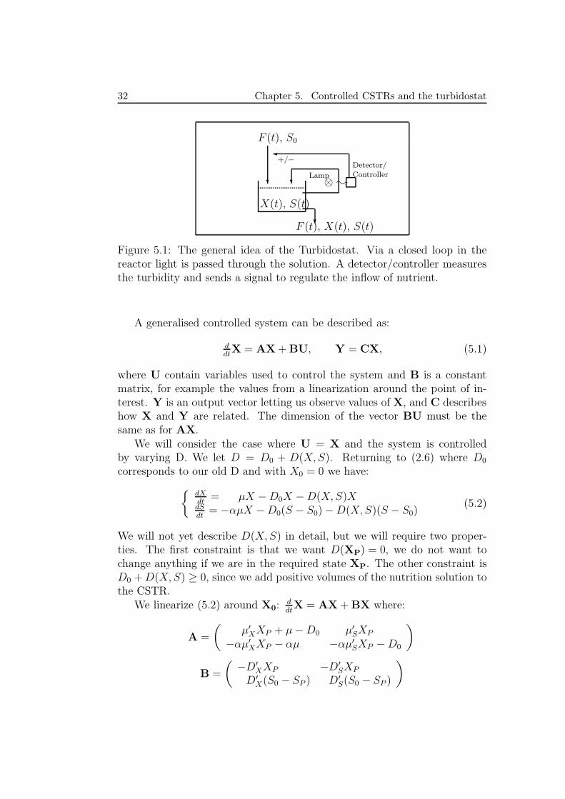
There are many ways to use automatic control in CSTRs to achieve goodresults. One general name for a class of controlled CSTR’s is auxostats.An auxostat is often defined as a continuous culture system in which theconcentration of one of the components, for example the pH-level, biomassconcentration, or nutrition concentration, is predetermined and the systemis controlled to maintain a constant level of this component.

One popular auxostat is the pH-auxostat since the active bacteria pro-duce organic acids as wasteproducts, lowering the pH. Measuring the pH ischeap and simple, and since pH is correlated to the productivity this type ofauxostat is easy to control.

Another auxostat is the turbidostat. The turbidity of a solution thatmeans how much light it absorbs is simple to measure, and is proportionalto the density of biomass X in the vessel. If there is too much density moresolution is added, and vice versa.

In general we want to fix our X at a value XP, a point in the proximity ofthe uncontrolled systems steady state X0. By doing this we assume that thebehaviour of the system is the similar to its behaviour in the neighbourhoodof X0, even if this might be at some distance from X0.


32 Chapter 5. Controlled CSTRs and the turbidostat

?

F (t), S0

?Lamp

⊗ ;

+/−Detector/Controller

X(t), S(t)

?

F (t), X(t), S(t)

Figure 5.1: The general idea of the Turbidostat. Via a closed loop in thereactor light is passed through the solution. A detector/controller measuresthe turbidity and sends a signal to regulate the inflow of nutrient.

A generalised controlled system can be described as:

ddtX = AX + BU, Y = CX, (5.1)

where U contain variables used to control the system and B is a constantmatrix, for example the values from a linearization around the point of in-terest. Y is an output vector letting us observe values of X, and C describeshow X and Y are related. The dimension of the vector BU must be thesame as for AX.

We will consider the case where U = X and the system is controlledby varying D. We let D = D0 + D(X, S). Returning to (2.6) where D0

corresponds to our old D and with X0 = 0 we have:

dXdt

= µX − D0X − D(X, S)XdSdt

= −αµX − D0(S − S0) − D(X, S)(S − S0)(5.2)

We will not yet describe D(X, S) in detail, but we will require two proper-ties. The first constraint is that we want D(XP) = 0, we do not want tochange anything if we are in the required state XP. The other constraint isD0 + D(X, S) ≥ 0, since we add positive volumes of the nutrition solution tothe CSTR.

We linearize (5.2) around X0:ddtX = AX + BX where:

A =

(µ′

XXP + µ − D0 µ′SXP

−αµ′XXP − αµ −αµ′

SXP − D0

)

B =

(−D′

XXP −D′SXP

D′X(S0 − SP ) D′

S(S0 − SP )

)

5.2. Invariant line for CSTRs controlled with D 33

This expression can now be used to derive convenient forms of controlledCSTRs.

Two important questions about controlled systems is their controllabilityand stabilisability. A system that is controllable is also stabilisable. By con-trollability we mean that a system, through a control policy, can be forced tomove from an initial state Xi to a desired state Xd in finite time. Control-lability in this case is guaranteed when det[B AB . . . An−1B] 6= 0, andis not obtained for the turbidostat. This means that not all states can beobtained in finite time.

Stabilisability is obtained when all eigenvalues of A can be made negativeby choosing a suitable control, but it may happen that eigenvalues of A

are negative from the beginning. This situation corresponds to our normalstability condition when the trace is negative and the determinant is positive.

5.2 Invariant line for CSTRs controlled with

D

As for the uncontrolled systems we can examine ddt

(S + αX). We end upwith:

d

dt(S + αX) = −(S + αX − S0) (D0 + D(X, S))

︸︷︷︸

≥0

Thus if the equality αX = S0 −S is fulfilled, we tend to keep it fulfilled: theminus sign in this relation ensures that we return to the invariant line if wefor some reason were to move away from it.

So there is an invariant line for CSTRs controlled with D and it is thesame as for the uncontrolled CSTRs.

5.3 The turbidostat

We will now look at the case where D(X, S) = D(X) = KD(X −XP ). XP isthe value of X we want to stabilize our CSTR about. If we apply µ = µ(S),we have µ′

X = 0. Also: D′S = 0 and D′

X = KD. The system is then:

dXdt

= µX − D0X − KD(X − XP )XdSdt

= −αµX − D0(S − S0) − KD(X − XP )(S − S0)(5.3)

This expression can be analyzed to learn how the controller action acts inthis case. If we search for a steady-state value of X we can ignore the trivial


steady state and end up with:

KDX = µ − D0 + KDXP ⇔

µ = D0, KD = 0

X = XP + µ−D0

KD, 0 < XP < ∞

X ≈ XP , KD ≫ µ − D0

KD is the key here: without control action (KD = 0) we return to Monodschemostat, for extremely large values of KD we end up with X = XP . Forreasonable values of KD we are close to XP . This middle expression alsocorresponds to a nullcline.

By linearizing (5.3) we get:

d

dtX = (A + B)X =

(µ − D0 − KDXP µ′

SXP

−αµ + KD(S0 − SP ) −αµ′SXP − D0

)

X

Now, sufficiently close to the steady state we can approximate D0 ≈ µ,allowing us to do some changes:

d

dtX ≈

(−KDXP µ′

SXP

−αµ + KD(S0 − SP ) −αµ′SXP − µ

)

X

As usual we want to know if this controlled system is stable and investi-gate the trace and the determinant:

tr(A + B) = −KDXP − αµ′SXP − µ

If µ is strictly growing (and its derivative positive) then indeed tr(A + B) <0. But if we for example have a CSI-CSTR µ′

S might be negative. A sufficientcondition is however KD > −αµ′

S.

If we assume that we are close to the invariant line and can use αXP ≈

S0 − SP , we get the determinant:

det(A + B) = µ′SKDXP (αXP − (S0 − SP ))

︸︷︷︸

≈0

+KDXP µ + XP µ(αµ′S + KD)

det(A + B) ≈ KDXP µ + XPµ(αµ′S + KD)

So we have a positive determinant if KD > −αµ′S, or if we have µ′

S > 0. Thissystem is thus stable. But since we do not have controllability we are notreally sure where we arrive to in the phase-plane.

5.4. The phaseportrait of a turbidostat 35

0 0.1 0.2 0.3 0.4 0.5 0.6 0.7 0.80

0.5

1

1.5

2

X

S

Figure 5.2: A phaseportrait of a Turbidostat. The diagonal dotted lineis the invariant line, the vertical dotted line corresponds to X = XP , thepoint-dotted line is an Euler path starting in (0.73, 2.2) and the full line anX-nullcline. The ring on the invariant line is where the steady state wouldhave been without the controller action. The arrows represent the vector-fieldcomposed of dX

dtand dS

dt.

5.4 The phaseportrait of a turbidostat

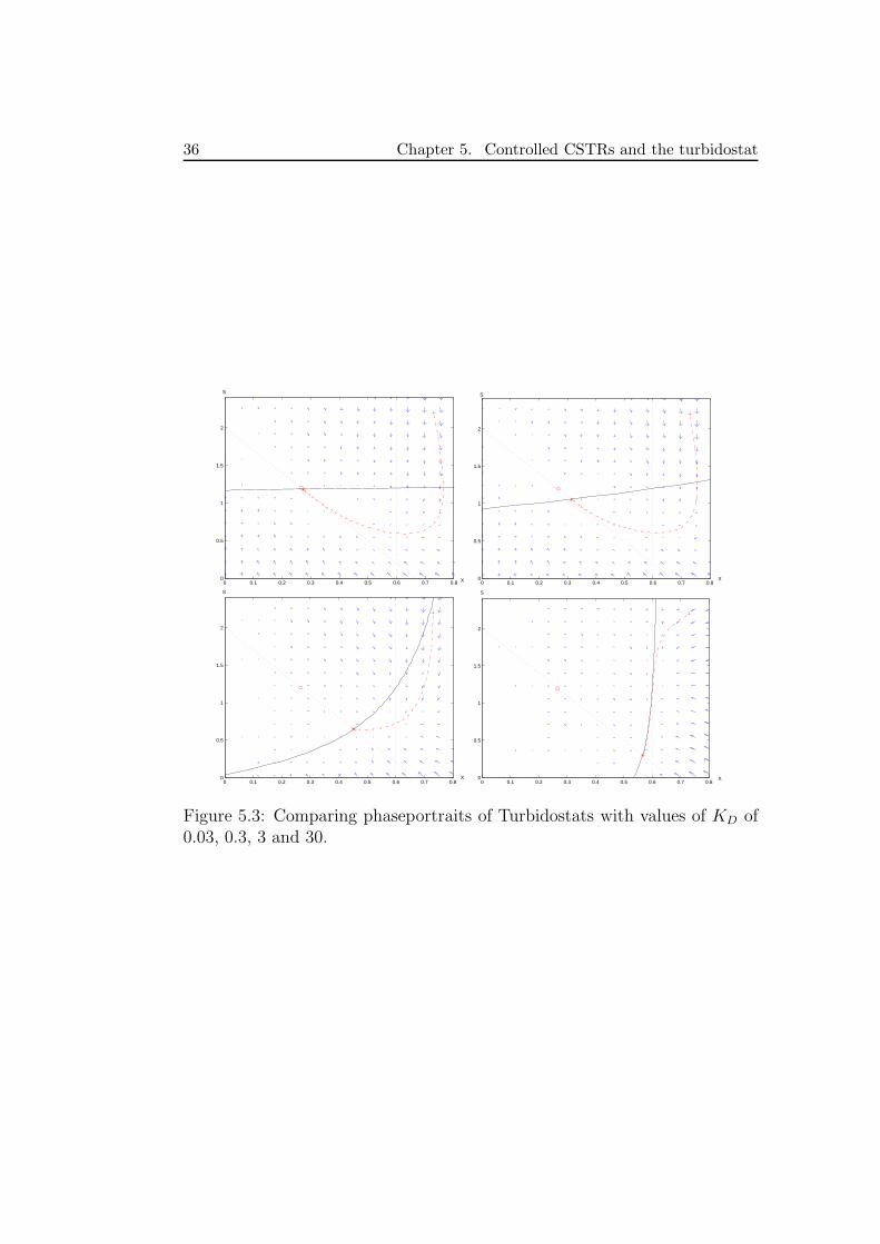
Looking at the phaseportrait of a Turbidostat, figure 5.2, the first strikingdifference is the distance between the normal chemostat steady state andthe steady state of the turbidostat. But here there is also an invariant lineas before and a nullcline in about the same place as before. This nullclinedepends however strongly on KD.

In figure 5.3 we see how the phase portrait changes with increasing valuesof KD: the nullcline tends to approach the line X = XP and thus the steadystate approaches the intersection of the null cline and of the invariant line.


0 0.1 0.2 0.3 0.4 0.5 0.6 0.7 0.80

0.5

1

1.5

2

S

X 0 0.1 0.2 0.3 0.4 0.5 0.6 0.7 0.80

0.5

1

1.5

2

X

S

0 0.1 0.2 0.3 0.4 0.5 0.6 0.7 0.80

0.5

1

1.5

2

S

X 0 0.1 0.2 0.3 0.4 0.5 0.6 0.7 0.8

0

0.5

1

1.5

2

S

X

Figure 5.3: Comparing phaseportraits of Turbidostats with values of KD of0.03, 0.3, 3 and 30.

Chapter 6

Summary and conclusion

In this report several mathematical models of bacteria population growth inbioreactors were analyzed.

In chapter 2 we explored two simple models of biological growth: expo-nential growth and by taking into account the substrate concentration,S, the logistic equation. The exponential growth is typically seen whenresources are good and the population is very small. The logistic equa-tion explains how a population is restricted by limited resources.

We introduced the in- and outflow of nutrient in our reactor, theMichaelis-Menten kinetics and analyzed Monods Chemostat. Equilib-rium solutions, nullclines, the parameters α1 and α2 and the phasepor-trait are found to be useful characteristics.

Chapter 3 is dedicated to the new model proposed: the Michaelis-Menteninhibited CSTR. The MMI-CSTR exhibits different phaseportrait show-ing how the MMI-CSTR responds to large values of X by inhibition.

A comparison of this model and Monods chemostat with the competi-tive substrate and product inhibition has been made.

In chapter 4 we discuss chemostats in series, a chemostat with recircu-lation and three chemostat-like enzyme reactors. We saw that in thechemostat with recirculation we could achieve µ > D, and that chemostatsin series allow us to take into account different ambient conditions forthe bacteria.

In chapter 5 we have explained how a controlled CSTR works and investi-gated the turbidostat: it illustrates a simple way of controlling a CSTR.


38 Chapter 6. Summary and conclusion

Bibliography

[1] Leah Edelstein-Keshet, (1988), Mathematical Models in Biology, Mc-Graw Hill, Inc.

[2] Harvey W. Blanch, Douglas S. Clark, (1997), Biochemical Engineering,Marcel Dekker, New York.

[3] Carl-Fredrik Mandenius, (2002), Industriell Bioteknik, Bokakademin,Linkoping.

[4] Colin Ratledge, Bjørn Kristiansen, (2001), Basic Biotechnology, Cam-bridge University Press, Cambridge.

[5] Lennart Rade, Bertil Westergren, (2001), Mathematics Handbook forScience and Engineering (BETA), Studentlitteratur, Lund.

[6] Pramod Agrawal, Henry C. Lim, Analyses of various control schemes forContinuous bioreactors, Adv. Biochem. Eng, Biotech 30, (1984) 91-90.

[7] Steven P. Fraleigh, Henry R. Bungay, Lenore S. Clesceri, Continuousculture, feedback control and auxostats, Tibtech, June 1989 [Vol. 7].

[8] Torkel Glad, Lennart Ljung, (1989), Reglerteknik grundlaggande teori,Studentlitteratur, Lund.


40 Bibliography

Appendix A

The Linearized stability

A.1 The Linearization

F (x), a one-variable function of x can be Taylor-expanded around a fix X.We get F (X + x) = F (X) + F ′(X)x + O(x2). For small perturbations of xaround X we get the linearization: F (X + x) ≈ F (X) + F ′(X)x, containingonly the constant and the linear terms.

For functions of two variables F (X + x, S + s) and G(X + x, S + s):

F (X + x, S + s) = F (X, S) + F ′X(X, S)x + F ′

S(X, S)s + O((x + s)2)

G(X + x, S + s) = G(X, S) + G′X(X, S)x + G′

S(X, S)s + O((x + s)2)

If F (x, s) = dXdt

, G(x, s) = dSdt

and the point (X, S) is an equilibrium pointthen the linearization is:

dXdt

= F (X + x, S + s) ≈ F′

X(X, S)x + F′

S(X, S)s = a11x + a12s

dSdt

= G(X + x, S + s) ≈ G′

X(X, S)x + G′

S(X, S)s = a21x + a22s

A convenient notation is ddtX ≈ AX =

(a11 a12

a21 a22

)

X, and is often used

when looking at the chemostat or other dynamical systems of similar math-ematical form.

A.2 The Stability

Now, let us use our linearization and look at some conditions needed for thelinearization to be stable. We have d

dtX = AX. Supposing that

x = c1 · v1eλ1t + c2 · v2e

λ2t we get, for each λ: ddtX = λAeλt = Aveλt.


42 Appendix A. The Linearized stability

Eliminating the exponential in the two last terms, we get the well-knownequation: det(A − λI) = 0 that has two solutions:

λ =a11 + a22

2±

√

4(a12a21 − a11a22) + (a11 + a22)2

2⇔

λ =tr(A)

2±

√

−4det(A) + tr(A)2

2

In order to have stable solutions we must have Re(λ) < 0 and thus tr(A) < 0.If we assume that tr(A) < 0 and look at the first λ (with a plus), we getλ1 < 0 ⇔

tr(A)

2+

√

−4det(A) + tr(A)2

2< 0 ⇔ 0 < det(A)

Thus, for us to not have a positive real part in our exponentials, we haveto have: tr(A) < 0 and det(A) > 0. This allows us to simply look at ourlinearization to know a lot of our how our system behaves near an equilibriumpoint.

Worth noting is also if the term√

−4det(A) + tr(A)2 is real or complex.

If a λ has a negative real part and no complex part in an equilibrium-point,this point could be considered to be a stable node because the exponentialsinclude only negative real numbers.

If λ contains some complex parts we can easily discover that the pairof λ’s must be complex-conjugated and that the exponentials give rise of aspiral-like motion in the (X,S)-plane around the equilibrium-point. We callthe point a stable spiral if tr(A) < 0.

Appendix B

A Matlab M-file

This appendix displays a Matlab M-file used to visualize the phase portrait andto control calculations. This example explains the principle, and it is easy tochange, for example, the kinetic expression to fit another model.

function chemostat_inhibited(alpha1, alpha2, xp0, sp0, xc)

%

%chemostat_inhibited Displays a phaseportrait, nullclines

% and an Euler-path of an inhibited Chemostat.

% chemostat_inhibited(alfa1, alfa2, np0, cp0, nc) will run if

% alpha1 > 1/xc, thus there is a reproduction.

% alpha2 > 1/(xc*alpha1-1), thus there is sufficient stock-nutrition.

% xp0 > 0 , you can not have a nonpositive population.

% sp0 > 0 , you can not have a nonpositive concentration.

% xc > 0

%

% The blue arrows represent the vectorfield.

% The black lines are two of the three nullclines.

% The black dotted line is the invariant line (no solution crosses it).

% The red line is an Eulerpath, starting in + and ending in *.

%

% Try the following:

% chemostat_inhibited(5, 3, 0.2, 0.3, 6)

%

% by Per Erik Strandberg, 2003-2004.

%

% Start-condition:

%------------------

if ((alpha1>1) & (alpha2>0) & (sp0>0) & (xp0>0) & xc>0),

if (alpha2<1/(alpha1-1)),

disp(’ ’)

disp (’ (HINT: Only the trivial steady state, alpha2 is too small...)’)

else

disp(’ ’)

disp (’ (HINT: Two steady states, alpha2 is quite large...)’)

end

% The non-trivial equilibrium-solution:

%-----------------------------------------


44 Appendix B. A Matlab M-file

a = (xc+1-alpha2-xc/alpha1);

b = (-alpha2-xc/alpha1);

sbar = -a/2 + sqrt(0.25*a*a-b) ;

xbar = -alpha1*sbar+alpha1*alpha2 ;

hold off

plot(xbar, sbar, ’rO’)

hold on

plot(0, alpha2, ’rO’)

% The vector-field:

%--------------------

[xx,ss]=meshgrid(0.01 : (alpha1*alpha2*1.3/15) : alpha1*alpha2*1.3 ,

0.01 : (alpha2*1.3/15) : alpha2*1.3);

dx= (alpha1*xx.*ss./(ss+1))./(1+xx./xc)-xx;

ds= -(xx.*ss./(ss+1))./(1+xx./xc)-ss+alpha2;

quiver(xx,ss,dx,ds, 1)

% One of the x-nullclines:

%----------------------------

x_x_nullcline=[0.001: (- (1-alpha1)*xc)*0.9/100 : - (1-alpha1)*xc*0.999];

c_x_nullcline = (1 + x_x_nullcline./xc) ./ (alpha1 - 1 - x_x_nullcline ./ xc) ;

plot(x_x_nullcline,c_x_nullcline,’k’)

% The s-nullcline:

%------------------

s5 = [(-0.5*(xc+1-alpha2) + sqrt(0.25*(-xc-1+alpha2)^2+alpha2))*1.001

: ((alpha2*0.999)-((-0.5*(xc+1-alpha2) +

sqrt(0.25*(-xc-1+alpha2)^2+alpha2))*1.001))/100

: alpha2*0.999];

x5 = xc*((alpha2-s5).*(1+s5)) ./ (xc*s5 -(alpha2-s5).*(1+s5));

plot(x5,s5,’k’)

% The Invariant line:

%-------------------------

s_inv=[0: alpha2/3 :alpha2];

x_inv=alpha1*alpha2 - alpha1*s_inv;

plot(x_inv,s_inv,’:k’)

% The Euler-path:

%------------------

xp=[1:1:1000];

sp=[1:1:1000];

xp(1)=xp0;

sp(1)=sp0;

i=1;

while i < 1000,

xp(i+1)=xp(i)+0.005*((alpha1*xp(i)*sp(i)/(sp(i)+1))./(1+xp(i)/xc)-xp(i));

sp(i+1)=sp(i)+0.005*(((-1)*xp(i)*sp(i)/(sp(i)+1))./(1+xp(i)/xc)-sp(i)+alpha2)

i=i+1;

end

plot(xp,sp,’r-.’)

plot(xp(1), sp(1),’r’)

plot(xp( 1), sp( 1), ’r+’)

plot(xp(1000), sp(1000), ’r*’)

%fixing the axis

45

%----------------

axis([0 alpha1*alpha2*1.2 0 alpha2*1.2 ])

disp(’ chemostat_inhibited.m by Per Erik Strandberg, 2003-2004. Finished OK.’)

disp(’ ’)

% The illegal indata case:

%---------------------------

else

disp(’ chemostat_inhibited.m by Per Erik Strandberg, 2003-2004.’)

disp(’ Did not Finish OK. (You used illegal indata.)’)

disp(’ ’)

disp(’ For syntax help type: help chemostat_inhibited .’)

disp(’ ’)

end

46 Appendix B. A Matlab M-file

LINKÖPING UNIVERSITY

ELECTRONIC PRESS

Copyright

The publishers will keep this document online on the Internet - or itspossible replacement - for a period of 25 years from the date of publica-tion barring exceptional circumstances. The online availability of the doc-ument implies a permanent permission for anyone to read, to download, toprint out single copies for your own use and to use it unchanged for anynon-commercial research and educational purpose. Subsequent transfers ofcopyright cannot revoke this permission. All other uses of the documentare conditional on the consent of the copyright owner. The publisher hastaken technical and administrative measures to assure authenticity, securityand accessibility. According to intellectual property law the author has theright to be mentioned when his/her work is accessed as described above andto be protected against infringement. For additional information about theLinkoping University Electronic Press and its procedures for publication andfor assurance of document integrity, please refer to its WWW home page:http://www.ep.liu.se/

Upphovsratt

Detta dokument halls tillgangligt pa Internet - eller dess framtida ersattare- under 25 ar fran publiceringsdatum under forutsattning att inga extraordi-nara omstandigheter uppstar. Tillgang till dokumentet innebar tillstand forvar och en att lasa, ladda ner, skriva ut enstaka kopior for enskilt bruk och attanvanda det oforandrat for ickekommersiell forskning och for undervisning.Overforing av upphovsratten vid en senare tidpunkt kan inte upphava dettatillstand. All annan anvandning av dokumentet kraver upphovsmannensmedgivande. For att garantera aktheten, sakerheten och tillganglighetenfinns det losningar av teknisk och administrativ art. Upphovsmannens ideellaratt innefattar ratt att bli namnd som upphovsman i den omfattning som godsed kraver vid anvandning av dokumentet pa ovan beskrivna satt samt skyddmot att dokumentet andras eller presenteras i sadan form eller i sadant sam-manhang som ar krankande for upphovsmannens litterara eller konstnarligaanseende eller egenart. For ytterligare information om Linkoping UniversityElectronic Press se forlagets hemsida http://www.ep.liu.se/

c© 2004, Per Erik Strandberg


strandberg thesis 200419668/... · · 2006-03-30per erik strandberg lith - mai - ex - - 04 / 04...

Documents