lith - mai - ex - - 04 / 04 - - se - per erik strandberg - startsidan · ·...

Examensarbete

Mathematical models of bacteria population growth in

bioreactors: formulation, phase space pictures, optimisation

and control.

Per Erik Strandberg

LiTH - MAI - EX - - 04 / 04 - - SE

Mathematical models of bacteria population growth in

bioreactors: formulation, phase space pictures, optimisation

and control.

Applied Mathematics, Linkopings Univeritet

Per Erik Strandberg

LiTH - MAI - EX - - 04 / 04 - - SE

Examensarbete: 20 p

Level: D

Supervisor: Stefan Rauch,Applied Mathematics, Linkopings Universitet

Examiner: Stefan Rauch,Applied Mathematics, Linkopings Universitet

Linkoping: March 2004

Matematiska Institutionen581 83 LINKOPINGSWEDEN

march 2004

x

x

http://www.ep.liu.se/exjobb/mai/2004/tm/004/

LiTH - MAT - EX - - 04 / 04 - - SE

Mathematical models of bacteria population growth in bioreactors: formulation, phasespace pictures, optimisation and control.

Per Erik Strandberg

There are many types of bioreactors used for producing bacteria populations in com-mercial, medical and research applications. This report presents a systematic discus-sion of some of the most important models corresponding to the well known reproduc-tion kinetics such as the Michaelis-Menten kinetics, competitive substrate inhibitionand competitive product inhibition.We propose a modification of a known model, analyze it in the same manner as knownmodels and discuss the most popular types of bioreactors and ways of controlling them.This work summarises much of the known results and may serve as an aid in attemptsto design new models.

Chemostat, Continuous Stirred Tank Bioreactors (CSTR), Dynamical Systems, Math-ematical Models in Biology, Biologic growth and Biologic production.

Nyckelord

Keyword

Sammanfattning

Abstract

Forfattare

Author

Titel

Title

URL for elektronisk version

Serietitel och serienummer

Title of series, numbering

ISSN0348-2960

ISRN

ISBNSprak

Language

Svenska/Swedish

Engelska/English

Rapporttyp

Report category

Licentiatavhandling

Examensarbete

C-uppsats

D-uppsats

Ovrig rapport

Avdelning, Institution

Division, Department

Datum

Date

Abstract

There are many types of bioreactors used for producing bacteria populations incommercial, medical and research applications. This report presents a system-atic discussion of some of the most important models corresponding to the wellknown reproduction kinetics such as the Michaelis-Menten kinetics, competitivesubstrate inhibition and competitive product inhibition.

We propose a modification of a known model, analyze it in the same manneras known models and discuss the most popular types of bioreactors and waysof controlling them. This work summarises much of the known results and mayserve as an aid in attempts to design new models.

Keywords: Chemostat, Continuous Stirred Tank Bioreactors (CSTR), Dy-namical Systems, Mathematical Models in Biology, Biologic growth andBiologic production.

Abstract in Swedish: Sammanfattning

Det finns manga typer av bioreaktorer som tillampas kommersiellt, och inommedicin och forskning. Denna rapport presenterar en systematisk redovisningav nagra av de viktigaste modellerna som motsvarar de kanda kinetiska for-merna Michaelis-Menten kinetik, kompetitiv substratinhibering och kompetitivproduktinhibiering.

Vi foreslar en modifiering av en kand modell, analyserar den pa samma sattsom kanda modeller och redogor for de popularaste bioreaktortyperna och hurde kan kontrolleras. Detta verk sammanfattar mycket av idag kanda resultatoch kan anvandas som hjalp i design av nya modeller.

Strandberg, 2004. vii

Acknowledgements

I would like to thank my supervisor and examiner Stefan Rauch, at the divisionof applied mathematics for his excellent guidance, our rewarding discussions andhis constant feedback.

I also have to thank Berkant Savas for helping to mature mathematically,for introducing me to the wonderful world of LATEX, and for his efforts in proof-reading this material.

My opponent Andreas Andersson also deserves my thanks for his construc-tive feedback and help in proofreading.

Strandberg, 2004. ix

Nomenclature

Most of the reoccurring abbreviations and symbols are described here.

Symbols

Y0 The amount of the variable Y inserted into a system.

Y The unit-dimension of the variable Y , for example t = 1s .Yi A steady state (number i) value of Y.

Ki Constants used in kinetic expressions, for example KI .

A The system matrix.a, b Growth- and non growth-associated production yield coefficients.c, ϕ, δ Fraction of X , F or S0. 0 < c < 1, 0 < ϕ < 1, 0 < δ < 1 .C, R The set of complex and real numbers.D Dilution coefficient; fraction of V replaced per timeunit.E Enzyme concentration in a system.F The flow of a media in or out of a system.P Product concentration in a system.S Substrate concentration in a system.V The volume of a system.X Biomass concentration in a system (kilogram/litre, etc.)X Vector containing S, X and P .

α1 Dimensionless maximal reproduction rate.α2 Dimensionless nutrition feed concentration.α, β Unitconsumtion of S needed to produce one unit of X or P .µ The general rate expression. µ = µ(S, X , P , . . . )

Abbreviations

CPI Competitive Product Inhibition (or Inhibited)CSI Competitive Substrate Inhibition (or Inhibited)CSTR Continuous Stirred Tank (bio)ReactorMMI Michaelis-Menten Inhibition (or Inhibited)

Strandberg, 2004. xi

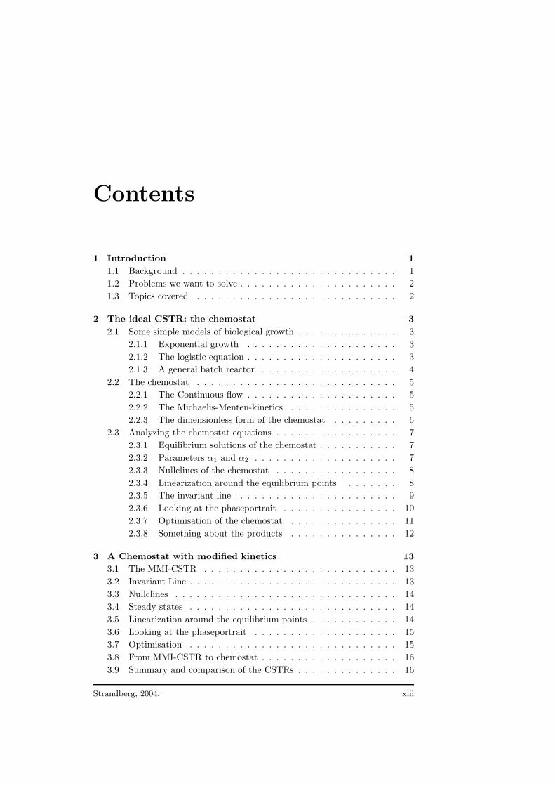
Contents

1 Introduction 1

1.1 Background . . . . . . . . . . . . . . . . . . . . . . . . . . . . . . 1

1.2 Problems we want to solve . . . . . . . . . . . . . . . . . . . . . . 2

1.3 Topics covered . . . . . . . . . . . . . . . . . . . . . . . . . . . . 2

2 The ideal CSTR: the chemostat 3

2.1 Some simple models of biological growth . . . . . . . . . . . . . . 3

2.1.1 Exponential growth . . . . . . . . . . . . . . . . . . . . . 3

2.1.2 The logistic equation . . . . . . . . . . . . . . . . . . . . . 3

2.1.3 A general batch reactor . . . . . . . . . . . . . . . . . . . 4

2.2 The chemostat . . . . . . . . . . . . . . . . . . . . . . . . . . . . 5

2.2.1 The Continuous flow . . . . . . . . . . . . . . . . . . . . . 5

2.2.2 The Michaelis-Menten-kinetics . . . . . . . . . . . . . . . 5

2.2.3 The dimensionless form of the chemostat . . . . . . . . . 6

2.3 Analyzing the chemostat equations . . . . . . . . . . . . . . . . . 7

2.3.1 Equilibrium solutions of the chemostat . . . . . . . . . . . 7

2.3.2 Parameters α1 and α2 . . . . . . . . . . . . . . . . . . . . 7

2.3.3 Nullclines of the chemostat . . . . . . . . . . . . . . . . . 8

2.3.4 Linearization around the equilibrium points . . . . . . . 8

2.3.5 The invariant line . . . . . . . . . . . . . . . . . . . . . . 9

2.3.6 Looking at the phaseportrait . . . . . . . . . . . . . . . . 10

2.3.7 Optimisation of the chemostat . . . . . . . . . . . . . . . 11

2.3.8 Something about the products . . . . . . . . . . . . . . . 12

3 A Chemostat with modified kinetics 13

3.1 The MMI-CSTR . . . . . . . . . . . . . . . . . . . . . . . . . . . 13

3.2 Invariant Line . . . . . . . . . . . . . . . . . . . . . . . . . . . . . 13

3.3 Nullclines . . . . . . . . . . . . . . . . . . . . . . . . . . . . . . . 14

3.4 Steady states . . . . . . . . . . . . . . . . . . . . . . . . . . . . . 14

3.5 Linearization around the equilibrium points . . . . . . . . . . . . 14

3.6 Looking at the phaseportrait . . . . . . . . . . . . . . . . . . . . 15

3.7 Optimisation . . . . . . . . . . . . . . . . . . . . . . . . . . . . . 15

3.8 From MMI-CSTR to chemostat . . . . . . . . . . . . . . . . . . . 16

3.9 Summary and comparison of the CSTRs . . . . . . . . . . . . . . 16

Strandberg, 2004. xiii

xiv Contents

4 Other CSTR-types 19

4.1 Chemostats in series . . . . . . . . . . . . . . . . . . . . . . . . . 194.2 Chemostat with recirculation . . . . . . . . . . . . . . . . . . . . 204.3 Chemostat-like enzyme reactors . . . . . . . . . . . . . . . . . . . 21

5 Controlled CSTRs and the turbidostat 23

5.1 Controlled CSTRs . . . . . . . . . . . . . . . . . . . . . . . . . . 235.2 Invariant line for CSTRs controlled with D . . . . . . . . . . . . 255.3 The turbidostat . . . . . . . . . . . . . . . . . . . . . . . . . . . . 255.4 The phaseportrait of a turbidostat . . . . . . . . . . . . . . . . . 26

6 Summary and conclusion 29

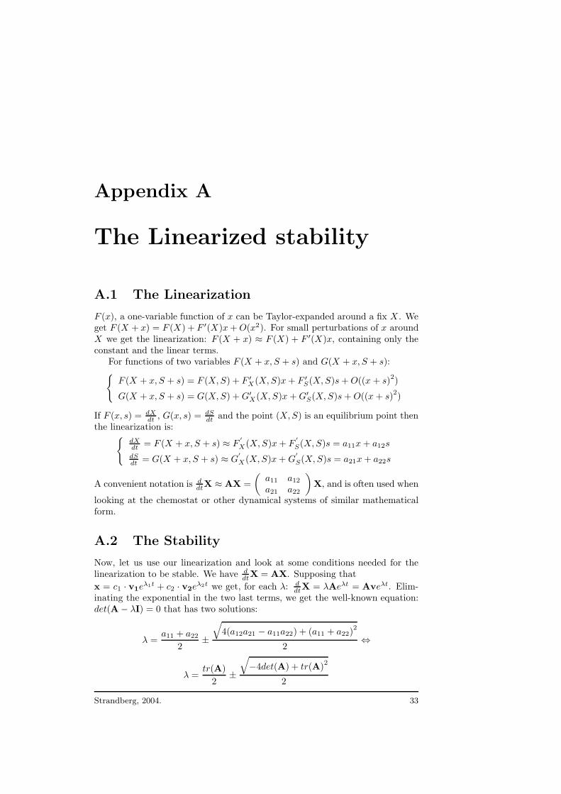
A The Linearized stability 33

A.1 The Linearization . . . . . . . . . . . . . . . . . . . . . . . . . . . 33A.2 The Stability . . . . . . . . . . . . . . . . . . . . . . . . . . . . . 33

B A Matlab M-file 35

Chapter 1

Introduction

This text is written as a master of science final thesis1 at the University of Linkopingby Per Erik Strandberg with Stefan Rauch as supervisor and examiner, with Emacsin LATEX in 2003/2004.

This first chapter will define what is a Continuous stirred tank bioreactor and achemostat. We give some background and formulate some main questions we wishto answer, and describe what topics are covered.

1.1 Background

Modeling of biological growth in reactors by dynamical systems started in the1950’s, when Monod, and Novick and Szilard developed the concept of Contin-uous Stirred Tank (bio)Reactors(CSTRs) that differed from traditional batchre-actors.

In a CSTR kinetics of the cellgrowth is sometimes referred to as a blackboxmodel , since all of the intra- and extra-cellular reactions are lumped into oneoverall reaction. Typical equations describing blackbox models are very similarto enzymatic kinetics (where there is often one substrate and one product inone reaction), such as the Michaelis-Menten kinetics used in the ideal CSTR(the chemostat), often referred to as Monods model.

?

-X , S, µ

F , X , S

S0, F

Figure 1.1: The ideal CSTR: the chemostat, its inflow of nutrition, its growth(µ), and its outflow.

1Swedish: Filosofie magister examensarbete.

Strandberg, 2004. 1

2 Chapter 1. Introduction

A chemostat is typically made of a reactor, containing a bacteria-population,of density X(t), and a substrate of density S(t) feeding the bacteria. The reactoris supplied with stocknutrient of concentration S0 from some kind of nutrientreservoir with the flow F that is constant over time. To maintain a constantvolume the inflow equals the outflow in which bacteria and/or products areharvested.

1.2 Problems we want to solve

This report provides a summary of already existing knowledge of bioreactorsand a detailed analysis of differential equations modelling bioreactors that oneusually encounters in textbooks. Some modifications of existing models areproposed and studied in detail.

This text aims to answer questions like “What types of bioreactors arethere?”, “If my bacteria population reproduces according to one of the kineticforms, how will it behave?”, “If my model is not really correct, how could Ichange it?”, “What do I need to consider before fixing my model?”, and somemore.

1.3 Topics covered

There are five chapters (and this introduction) and two appendixes. Main topicsdealt with are:

Chapter 2: We explain the chemostat equations with the standard Michaelis-Menten kinetics by starting with two simple models of biological growth.We also present some tools useful for studying dynamical systems in twodimensions.

Chapter 3: A new kinetic form is proposed and applied to an ideal CSTR.

Chapter 4: We leave the ideal CSTR and introduce, motivate and examinesome modified CSTRs.

Chapter 5: We look at controlled CSTRs.

Chapter 6: Summary and conclusion.

Appendix A: An appendix dealing with tools used to simplify the analysis oflinearized stability in steady states.

Appendix B: A Matlab M-file is appended, showing how a program like Mat-lab can be used to visualize and experiment with a given mathematicalmodel.

Chapter 2

The ideal CSTR: the

chemostat

In this chapter we study exponential growth, the logistic equation and the batchre-actors. We introduce the terminology, and explain how to think and how to lookat models and their describing differential equations.

We will derive and carefully analyze the chemostat equations. These equationswill constitute a reference model for the remaining parts of this text.

2.1 Some simple models of biological growth

2.1.1 Exponential growth

An extremely simple model could be dXdt = µ ·X where µ is the birth coefficient

and X stands for bacteria density. If µ = constant > 0, we get X(t) = X0eµt.

This is too simple a model. To limit the production of organisms we in-troduce a variable S describing concentration of the nutrient into the dynamicequations.

2.1.2 The logistic equation

Let us assume that dXdt = µ ·X, with µ = µ(S) = k ·S, and that dS

dt = −αkSX ,meaning that each unit of bacteria density produces kS units of offspring pertime unit. With α = constant > 0 we could mean that each produced unit ofoffspring requires α units of nutrition. This model corresponds to our intuition:the term SX says how often bacteria and food meet, giving the bacteria anopportunity to consume nutrient particles from the inflow S0 and to reproduce.

We get a system of ordinary differential equations:

dXdt = kSX (a)

dSdt = −αkSX (b)

Multiplying (a) by α and adding (b) we get: ddt (S + αX) = 0, thus (S +

αX)(t) = S0 + αX0 = constant. In particular with t = 0 and X(0) = X0 ≈ 0(or at least small in comparison to a normal X(t)) we have S(0)+ αX(0) ≈ S0,

Strandberg, 2004. 3

4 Chapter 2. The ideal CSTR: the chemostat

since X0 small implies S(t) = S0 − αX(t), giving us a reason to eliminate (b),and rewrite (a) as:

dX

dt= k(S0 − αX

︸︷︷︸

≈S(t)

)X = kS0︸︷︷︸

r>0

(1 −X

S0/α︸︷︷︸

B>0

)X = r(1 −X

B)X

By changing some factors we have reduced our system of ordinary differentialequations to a single equation, called the logistic equation:

dX

dt= r(1 −

X

B)X (2.1)

The factor r(1− XB ), that corresponds to our old µ, is called an intrinsic1 growth-

speed, and B the carrying capacity. By eliminating X instead of S, we quicklyfind dS

dt = −αr(1 − SαB )S, an equation describing time change of the nutrient

concentration.When analyzing (2.1) we discover that for small values of X , when 0 < X ≪ B

we can approximate (2.1) by an exponential term and our model gives exponen-tial growth for very small initial population densities.

The factor −XXB in the equation corresponds to a crowding effect, inhibiting

the reproduction rate.The sign of (1− X

B ) is important to analyze. Let us assume that X ≥ 0. We

also know that r > 0. Meaning that (1− XB ) is what determines the sign of dX

dt .

X = 0 ⇒ dXdt = 0, a trivial solution, there is no population;

0 < X < B ⇒ (1 − XB ) > 0, the population grows;

X = B ⇒ dXdt = 0, constant population; and

X > B ⇒ dXdt < 0, decreasing population.

We now know that the model corresponds to our intuition. A small popula-tion initially grows exponentially, later the term (1 − X

B ) starts to play role. Ifever X = B we will get a constant population. Finally: if X > B, N will even-tually diminish towards X = B. X = 0 and X = B are equilibrium solutions,or steady states.

An explicit solution to (2.1) is: X(t) = X0BX0+(B−X0)e−rt , if 0 < X0 < B. It

can be found by separating variables in equation (2.1)

2.1.3 A general batch reactor

Before we introduce the chemostat let us make a comment on a more generalcase that is similar to logistic growth: the batch reactor.

Into a vessel (reactor) we insert a nutrition solution with concentration S0

and a small population of bacteria X0 and close the lid. Assume we have somekind of kinetic expression µ. We then get the equations:

dXdt = µX (a)

dSdt = −αµX (b)

(2.2)

Again, as with the logistic growth we sum up α(a) + (b) and, for the samereasons as above, find: S = S0 + α(X0 −X). If we can assume X0 ≪ X we get

1Swedish: “inre” or “inneboende”

2.2. The chemostat 5

the nice, and general expression: S = S0 − αX . Again we can eliminate S and,if µ = µ(X), end up with:

dX

dt= µ(X) · X (2.3)

We can now insert various kinetics instead of µ and investigate what happens.

2.2 The chemostat

A chemostat is made of two main parts; a nutrient reservoir, and a growth-chamber, reactor, in which the bacteria reproduces. Via an inflow from thereservoir fresh nutrition is added and from an outflow bacteria are harvested.

The purpose of the chemostat is to have a quasi-constant X and S, allowingus to harvest at a constant rate. The name chemostat stands for “the chemicalenvironment is stat ic”.

We must adjust our earlier models by introducing an inflow and in doing so,we will also define units used in our growth-chamber.

We will also reduce the number of parameters of the chemostat by reducingit to the dimensionless form.

2.2.1 The Continuous flow

We let F = Fin = Fout having dimensions of volume/time. With Fin comes S0:“mass”/volume2. In the reactor we have a population of bacteria of density X :mass/volume, and S: mass/volume.

We modify equation (2.1) by adding terms describing the inflow of thenutrition-solution and the outflow of bacteria, and assume µ = µ(S). Thus:

dXdt = µ(S)X

new︷︸︸︷

−XF

VdSdt = −αµ(S)X −S

F

V+ S0

F

V︸︷︷︸

new

(2.4)

As we can see, F appears together with V in the form of F/V , so we setF/V = D - a dilution coefficient. It describes the fraction of volume beingreplaced in a unit of time.

The term X/V describes the density of bacteria, and by multiplying it withF we get the amount of bacteria being flushed away in a unit of time. Similarly−DS corresponds to the outflow of the nutrient, and +DS0 to the inflow of thenutrient.

2.2.2 The Michaelis-Menten-kinetics

We will now discuss the reproduction coefficient, µ(S), by relating it to theMichaelis-Menten kinetics. This is the main “black box” we will see, and it isoften also referred to as Monods kinetics.

Experimental data and similar cases in enzyme kinetics motivate the needof the reproduction-constant to be almost linear for small positive values for S,

2“Mass” could be moles, kilograms, molecules, etc.


but we also require an upper limit for µ so that: µ(S)S→∞−→ µmax. We write

down the Michaelis-Menten-kinetics:

µ(S) =µmaxS

KN + S

The new constant KN has an interesting meaning: KN

KN +KN= 1

2µmax. So

KN corresponds to the concentration at which µ = 12µmax

Let us see how µ(S) depends on S:Small S’s give us µ(S) ≈ S µmax

KN, if we can assume S ≪ KN , thus µ(S) is

almost linear. The maximum µ, µmax, is never reached, no matter how great Sgets, we have µ(S) < µmax.

The limit µ(S)S→∞−→ µmax is what we wanted. So µmax is the maximal

reproduction rate, achieved when the nutrient is unlimited.With this µ(S), the model becomes:

dXdt = µmax

SKN+S X − DX

dSdt = −αµmax

SKN+S X − DS + DS0

(2.5)

A more general CSTR, where Ω stands for other possible variables (X, (bi-)products, pH, . . . ) that may influence the reproduction rate, and X0 stands forbacteria density inserted via the in-flow, could be described by:

dXdt = µ(S, Ω)X − DX + DX0

dSdt = −αµ(S, Ω)X − DS + DS0

(2.6)

It is important to understand the structure of (2.6). We will look at othersCSTR’s, where this form is the common origin.

2.2.3 The dimensionless form of the chemostat

A quick glance at our equations show that we have a number of variable param-eters: µmax, KN , D, α, and S0. Each one of them is important and necessary,but is there a way for us to reduce the number of parameters somehow? Theanswer is yes, and we will see that it is possible to eliminate three of our con-stants (we eliminate five of them and introduce two new ones, this is possiblesince we have five parameters, and three dimensions).

As the title of this subsection suggests, we will actually eliminate the di-mensions/units of the equations, but first we must investigate the units of ourconstants. The first relation:

dim[dXdt ] = number

volume·time (here we assume dim[X ] = number/volume and

dim[t] = time), thus: dim[µmaxXSKN+S ] = number

volume·time . With dim[S] = massvolume we

get dim[KN ] = massvolume in order to keep KN + S meaningful, only allowing

dim[µmax] = 1time .

Our second relation: dim[dSdt ] = mass

volume·time , and since we know that dim[S] =mass

volume , we get dim[S0] = massvolume . So for α we get dim[α] = mass/volume

number/volume = 1.

And now, to simplify, we replace S, X , and t with S · S, X · X, and t · t.Where S, X and t corresponds to the unit-dimension, whatever they may be.3

3Note that t could be a second, a year, 3.25489677 minutes, etc, X could be one bacteria,twelve bacterias or 2.553 kg of dry cellweight per litre, gallon or tankvolume, and S couldtypically be: mol/l, molecules/mm3 or 3.333 lb/gallon.

2.3. Analyzing the chemostat equations 7

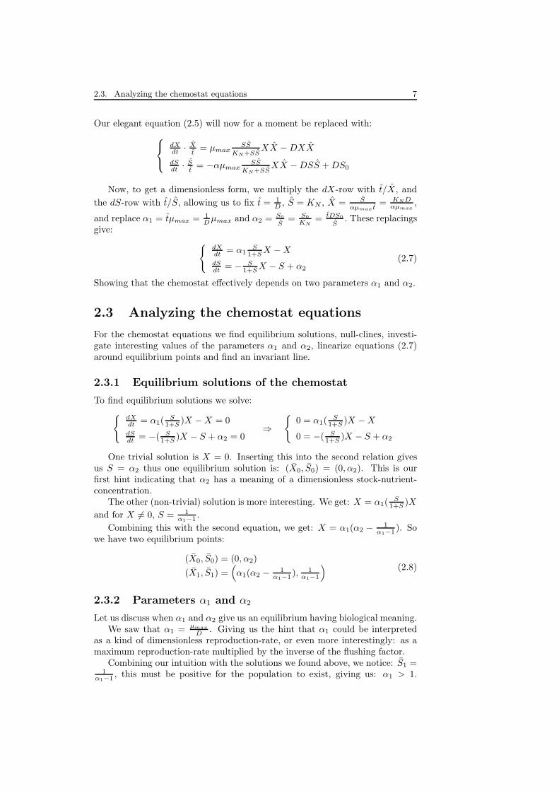
Our elegant equation (2.5) will now for a moment be replaced with:

dXdt · X

t= µmax

SSKN+SS

XX − DXX

dSdt · S

t= −αµmax

SSKN+SS

XX − DSS + DS0

Now, to get a dimensionless form, we multiply the dX-row with t/X, and

the dS-row with t/S, allowing us to fix t = 1D , S = KN , X = S

αµmax t= KN D

αµmax,

and replace α1 = tµmax = 1Dµmax and α2 = S0

S= S0

KN= tDS0

S. These replacings

give:

dXdt = α1

S1+S X − X

dSdt = − S

1+S X − S + α2

(2.7)

Showing that the chemostat effectively depends on two parameters α1 and α2.

2.3 Analyzing the chemostat equations

For the chemostat equations we find equilibrium solutions, null-clines, investi-gate interesting values of the parameters α1 and α2, linearize equations (2.7)around equilibrium points and find an invariant line.

2.3.1 Equilibrium solutions of the chemostat

To find equilibrium solutions we solve:

dXdt = α1(

S1+S )X − X = 0

dSdt = −( S

1+S )X − S + α2 = 0⇒

0 = α1(

S1+S )X − X

0 = −( S1+S )X − S + α2

One trivial solution is X = 0. Inserting this into the second relation givesus S = α2 thus one equilibrium solution is: (X0, S0) = (0, α2). This is ourfirst hint indicating that α2 has a meaning of a dimensionless stock-nutrient-concentration.

The other (non-trivial) solution is more interesting. We get: X = α1(S

1+S )X

and for X 6= 0, S = 1α1−1 .

Combining this with the second equation, we get: X = α1(α2 − 1α1−1 ). So

we have two equilibrium points:

(X0, S0) = (0, α2)

(X1, S1) =(

α1(α2 −1

α1−1 ), 1α1−1

)(2.8)

2.3.2 Parameters α1 and α2

Let us discuss when α1 and α2 give us an equilibrium having biological meaning.We saw that α1 = µmax

D . Giving us the hint that α1 could be interpretedas a kind of dimensionless reproduction-rate, or even more interestingly: as amaximum reproduction-rate multiplied by the inverse of the flushing factor.

Combining our intuition with the solutions we found above, we notice: S1 =1

α1−1 , this must be positive for the population to exist, giving us: α1 > 1.


Meaning that we must limit the dilution rate to be smaller than the maximalreproduction rate.

From the trivial solution we notice that S0 = α2 = S0

KNcharacterises nu-

trient. But as we will see, this is one way of dealing with α2. Another way oflooking at this parameter is to interpret it as an inverse number of KN , or asthe amount of S we have, measured in units of KN . We saw that a small KN

means that we are closer to µmax for lower values of S. So small KN meansthat α2 is large and vice versa.

Looking at our non-trivial solution again we notice that X1 = α2−1

α1−1 must

be positive for the population to exist. Requiring α2 > 1α1−1 . (Thus α2 > 0.)

Here we can see that for small (α1−1) (large flushing or weak reproduction) weneed α2 to be large (strong flushing or weak reproduction, requires more foodin order to reproduce faster), and a large α1 allows α2 to be small. This is howthe model tells us that if it easy to reproduce we have a lower need of nutrition.

2.3.3 Nullclines of the chemostat

A useful tool for investigating this kind of dynamic systems are nullclines, thelines where dX

dt = 0, or dSdt = 0. We also understand that at the crossing of two

different kind of nullclines there is an equilibrium point.

Let us begin with the X-relation: 0 = dXdt = α1(

S1+S )X − X, we notice that

one nullcline is: X = 0, and the other ones is: α1(S

1+S ) − 1 = 0 so S = 1α1−1 .

Continuing with the nullclines for S: 0 = dSdt = −( S

1+S )X −S +α2 = 0, after

some elementary work, we get: X = (α2−S)(1+S)S . Our nullclines are given by:

X = 0 ⇒ X = 0 or S = 1α1−1

S = 0 ⇒ X = (α2−S)(1+S)S

The nullclines are easy to draw, and by drawing some vectors in the firstquadrant, we can get a pretty good idea of how a state (X(t), S(t)) moves aroundin the (X,S)-plane over time.

2.3.4 Linearization around the equilibrium points

We have found two equilibrium solutions in the positive quadrant of the (X,S)-

plane: (X0, S0) = (0, α2) and (X1, S1) =(

α1(α2 − 1α1−1 ), 1

α1−1

)

. We want to

study in the neighbourhood of these points how the chemostat responds to smalldisturbances. Does it wander away from an equilibrium or does it fall back ontoit? The question we want to answer is: is the solution stable?

In order to analyze the chemostat’s behaviour at the equilibrium we will usethe stability conditions described in Appendix A. The stability conditions aretr(A) < 0 and det(A) > 0. For eigenvalues of the linearization matrix A to bereal we need −4 det(A) + tr(A)2 > 0.

We find (see Appendix A):

A =

(a11 a12

a21 a22

)

=

(

α1S

1+S − 1 α1X(1+S)2

− S1+S − X

(1+S)2− 1

)


Evaluating this at the trivial equilibrium point (X0, S0) = (0, α2) we get:

A =

( α1α2

1+α2− 1 0

− α2

1+α2−1

)

⇒

tr(A) = α1α2

1+α2− 2

det(A) = − α1α2

1+α2+ 1

We know that we have two conditions for stability around an equilibriumpoint: tr(A) < 0 and det(A) > 0. We will notice that our second condition:− α1α2

1+α2+ 1 > 0 ⇔ 1 > α1α2

1+α2is in conflict with the earlier condition for

physical meaning, α2 > 1α1−1 ⇔ 1 < α1α2

1+α2. So this steady state is not

stable.At the other equilibrium point, (X1, S1) =

(

α1(α2 − 1α1−1 ), 1

α1−1

)

, by re-

naming the term X1

(S1+1)2= σ and remember that σ > 0, we get:

A =

(0 σα1

− 1α1

−σ − 1

)

⇒

tr(A) = −σ − 1 < 0.det(A) = σ > 0.

The non-trivial equilibrium point is thus stable. We also note that:−4 det(A) + tr(A)

2= −4σ + σ2 + 2σ + 1 = σ2 − 2σ + 1 = (σ − 1)

2> 0. So

trajectories of a state near this point are not spiraling since their eigenvectorsare real. They go more straight-forward towards (X1, S1).

2.3.5 The invariant line

In this subsection we study the line X = −α1S + α1α2.

All solutions asymptotically approaches the invariant line

From (2.7):

dXdt = α1(

S1+S )X − X (a)

dSdt = −( S

1+S )X − S + α2 (b)we perform (a)+α1(b) and get:

ddt (X + α1S)(t) = α1α2 − (X + α1S)(t). We can look at this relation as anordinary differential equation with one function (X + α1S)(t). One solutionis: (X + α1S)(t) = Ke−t + α1α2. One nice property of (X + α1S)(t) is that

(X + α1S)(t)t→∞−→ α1α2.

Thus when t → ∞ we have X − α1S = α1α2 ⇔ X = −α1S + α1α2, allsolutions wandering in the positive quadrant of the (X,S)-plane asymptoticallyapproaches this line.

We also notice that putting X = 0 will give S = α2, the trivial equilibriumpoint, and S = 0 give us X = α1α2. You can also easily verify that this linepasses through the non-trivial equilibrium point as well.

The invariant line has the direction of one of the eigenvectors

We remember that A =

(0 σα1

− 1α1

−σ − 1

)

, σ = X1

(S1+1)2> 0, now assume

that a solution has the form:

(X(t)S(t)

)

= X(t) = veλt. When differentiating

this and looking at our linearization we get: Aveλt = λveλt, and when usingthe classic secular equation to find the eigenvalues and eigenvectors we get:

(A − Iλ)v = 0 ⇒ 0 = det(A − Iλ) = det

(−λ α1σ− 1

α1−σ − 1 − λ

)


⇒ λ(σ + 1 + λ) + σ = 0 ⇒ λ1 = −1, and λ2 = −σ.

Since we saw −4 det(A)+ tr(A)2

> 0 we had expected real eigenvalues and thestability conditions are fulfilled, so we had expected them to be negative. Nowwe must find the eigenvectors. We insert our eigenvalues in (A − Iλ)v = 0:

(A − Iλ1)v1 =

(1 α1σ

− 1α1

−σ

)(v11

v12

)

= 0 ⇒ v1 =

(α1σ−1

)

(A − Iλ2)v2 =

(σ α1σ

− 1α1

−1

)(v21

v22

)

= 0 ⇒ v2 =

(α1

−1

)

By elongating the eigenvector v2 in positive and negative directions from(X1, S1) we can easily verify that this is the same line as X = −α1S + α1α2.Thus a state starting on the invariant line can not move away from it.

An observation

By the theorem of existence and uniqueness of solutions of ordinary differentialequations two trajectories cannot cross each other. Thus the invariant line(consisting of trajectories) cannot be crossed. This helps in understanding howtrajectories behave in the neighbourhood of the invariant line (see figure 2.1).

The invariant line: conclusions

We can now conclude that the invariance line can be seen as a barrier for thesolutions. No solution above it can get below it and vice versa. This gives us aguidance in drawing a phase portrait, and we can see in the Matlab simulationthat, indeed, the solutions near the non-trivial equilibrium solution can notmove around in spirals.

2.3.6 Looking at the phaseportrait

When looking at the phaseportrait we will plot trajectories using Eulers method:Xn+1 = Xn + ∆t · d

dtXn. We can call this kind of trajectory an Euler path.

The phaseportrait of this kind of a system gives us a lot of information. Inthis example we can see the invariant line (dotted), the nullclines, and an Eulerpath (point-dotted) starting at a low amounts of both bacteria and nutritionrates. In this example we understand that the state at first wanders towardshigher amounts of nutrition (the bacteria are slowly reproducing). When thereis sufficient amounts of nutrition the state wanders off towards more bacteriaslowing the increase of nutrition, bending it off to the right then getting almostparallel to the invariant line, and finally asymptotically reaching the steadystate.

In figure 2.1 (and the following figures in later sections) we can see α2 wherethe invariant line crosses the S-axis (in the trivial steady state there are nobacteria and stock-concentration of nutrient). We can also find α1α2 at theinvariant lines crossing of the X-axis. From this information we can find thedimensionless units of X and S if we would like.


0 1 2 3 4 5 6 7 8 90

0.5

1

1.5

2

2.5

3

3.5

4

4.5

X

S

Figure 2.1: A phaseportrait of a chemostat. The dotted line is the invariantline, the point-dotted line an Euler path and the Continuous lines are nullclines(the S-axis is an X-nullcline). The arrows represent the vector-field (dX

dt , dSdt ).

Notice that the Euler path approaches the invariant line but never crosses it.

2.3.7 Optimisation of the chemostat

Now we will leave the dimensionless form and return to the general model,(2.6). We will adapt it to fit the chemostat, and express the steady states ina different way. We will do so since many of the parameters we changed infinding the dimensionless form includes the dilution coefficient D, and we needto compute d

dD (DX) in order to find an optimal value for D. The model is now:

dXdt = µX − DXdSdt = −αµX − DS + DS0

If we focus on the nontrivial steady state (ignoring the indexes): (X, S), wefind D = µ if we let dX

dt = 0, simplifying the relationdSdt = 0 = −αDX − DS +

DS0 ⇔ X = 1α (S0 − S).

For Monods kinetic expression, we let D = µ = µmaxS

KS+S⇔ S =

DKS

µmax−D , and now we can find an expression for X: X = 1α (S0 −

DKS

µmax−D ). Weare easily convinced that this expression multiplied with D is one way to measurethe amount of productivity, if we assume that productivity is growth-associated,or if we are interested in the bacteria in itself (as in the yeast-production).

Now we have Xout = XD and we want to maximize this, and find an op-

timum. We calculate ddD (XD) and find D = µmax(1 ±

√KS

S0+KS), but (as we

saw earlier) D = µ, so there is no way D could be greater than µmax, leaving

us with the only possible solution: Dmax = µmax(1 −√

KS

S0+KS) ⇒

Xout,max = 1α

(

S0 + KS −√

KS(S0 + KS))

.


2.3.8 Something about the products

So far, we have only considered a system where biomass and substrate concen-tration were described. Biomass, as for yeast production is usually the variableof interest. Sometimes, as for waste treatment, the substrate is what is inter-esting. But there is also the possibility that another variable P , the product, iswhat we want to know more about.

A common way to describe the change in product density is to assume thatthere are both growth- and non-growth-associated production. The growth-associated production is proportional to the ammount of growth by the constanta, and the non-growth-associated production to the bacteria density by theconstant b. We get the us the system:

dXdt = µX − DX

dSdt = D(S0 − S) − αµX − β(aµX + bX)

dPdt = aµX + bX − DP

(2.9)

We recognize α as the unit-consumption of S required to produce one unit of X ,and β as the unit-consumption of S required to produce one unit of P The “new”constants a and b describe the difference between growth-associated productionand non-growth-associated production respectively.

Looking for a nontrivial steady state we let dXdt = 0 and find µ = D, from

this we can usually find S if we have X, and P . P is found by taking µ = D anddPdt = 0 ⇒ P = aX+ bX

D . Finding X requires a little work, and we calculate:dSdt = 0 ⇔ X(αD + βaD + βb) = D(S0 − S) ⇔ X = S0−S

α+β(a+ bD

), so the

(non-trivial) steady state for a general µ is:

X = S0−Sα+β(a+ b

D)

P = aX + bXD

µ = D ⇒ S

If we are interested in S we can often easily find it from the above relations.If we use the only kinetics we have encountered so far, the Monod kinetics, weagain find: S = DKS

µmax−D and get:

S = DKS

µmax−D

X = S0−Sα+β(a+ b

D)

P = aX + bXD

As in Optimising Xout the Optimisation of P requires computing d(DP)dt = 0.

Chapter 3

A Chemostat with modified

kinetics

We have considered so far a chemostat with Monods kinetics. In this chapter wewill investigate our modification of this model.

Similarities with Monods equations will aid us in performing an analysis of theequations in a similar way as in Chapter 2.

3.1 The MMI-CSTR

We call this model the Michaelis-Menten inhibited Continuous stirred tank re-actor (MMI-CSTR) since we use a kind of Michaelis-Menten kinetics to lowerthe influence of growing values of X in the kinetic expression. We take the termµ = µmax

SKS+S

XKX+X in our equations instead of µmax

SKS+S X , as in Monods

chemostat. This kinetic form describes the situation when a high density, X , ofbacteria inhibits the growth in the chemostat.

By introducing the proposed inhibition we get the MMI-CSTR:

dXdt = µmax

SKS+S

XKX+X − XD

dSdt = −αµmax

SKS+S

XKX+X − SD + S0D

(3.1)

To obtain a nondimensional form we replace S, X and t with S · S, X · Xand t · t. We start by multiplying the relations with t/X and t/S respectively

then replace t = 1D , S = KS, X = S

α µmaxKX

t, and replace α1 = µmax

KXD and α2 = S0

S.

Finally, we let KX = XCX, to write the equations as:

dXdt = α1

S1+S

X1+ X

XC

− X

dSdt = − S

1+SX

1+ XXC

− S + α2

(3.2)

3.2 Invariant Line

As previously, we can find that X = α1(α2 − S) in an invariant line.

Strandberg, 2004. 13

14 Chapter 3. A Chemostat with modified kinetics

3.3 Nullclines

We let dXdt = 0 and find the line X = 0, but also S =

1+ XXC

α1−(1+ XXC

). Now, if

dSdt = 0 we get: X = (α2−S)(1+S)

S+ 1XC

(α2−S)(1+S). So the nullclines are:

dXdt = 0 ⇒ X = 0 or S =

1+ XXC

α1−(1+ XXC

)

dSdt = 0 ⇒ X = (α2−S)(1+S)

S+ 1XC

(α2−S)(1+S)

3.4 Steady states

Using the first of the dXdt = 0 nullclines we find the same trivial steady state:

(X0, S0) = (0, α2). If we use the second relation in combination with the invari-ant line to eliminate X we end up with the second degree equation:

S2 + S (XC + 1 −XC

α1− α2)

︸︷︷︸

p−q

+ (−XC

α1− α2)

︸︷︷︸

−q

= 0, with the solutions

S = q−p2 ±

√

( q−p2 )2 + q. One can quickly find that the solution with a minus

is negative, so we reject it. The other solution however must be smaller than α2

in order for the X associated to it to be positive, so the following assumptions

are needed: α2 > − p−q2 +

√

(p−q2 )2 + q ⇔ α2 > 1

α1−1 , for any non-trivial

steady state to exist. We also understand that α1 > 1. These conditions willbe used later.

3.5 Linearization around the equilibrium points

For the MMI-CSTR the system matrix A is:

A =

α1S

1+S1

(1+ XXC

)2− 1 α1

1(1+S)2

X1+ X

XC

− S1+S

1(1+ X

XC)2

− 1(1+S)2

X1+ X

XC

− 1

.

When we investigate the trace and the determinant at the steady states wemay use the relation: dX

dt = 0 ⇔ α1XS = X(1 + S)(1 + XXC

), to simplifythe matrix A (for X 6= 0):

A =

11+ X

XC

− 1 XS(1+S)

−1/α1

1+ XXC

−X/α1

S(1+S) − 1

=

− XXC

1+ XXC

XS(1+S)

−1/α1

1+ XXC

−X/α1

S(1+S) − 1

.

As we can see: trA < 0, but how about det(A), is it positive? We eliminatesome of our X by using the invariant line:

A =

− XXC

1+ XXC

α1(α2−S)S(1+S)

−1/α1

1+ XXC

−(α2−S)S(1+S) − 1

⇒

3.6. Looking at the phaseportrait 15

det(A) =X

XC

1 + XXC

( α2 − S

S(1 + S)+ 1)

+α2 − S

(1 + XXC

)(1 + S)> 0

Thus, the nontrivial steady state is stable.If we now study the trivial steady state, we have X = 0, so A is:

A =

(α1α2

1+α2− 1 0

− α2

1+α2−1

)

⇒

tr(A) = α1α2

1+α2− 2 ⇒ α1α2

1+α2< 2, for stability.

det(A) = −( α1α2

1+α2− 1) ⇒ α1α2

1+α2< 1, for stability.

So, we have to have α1α2

1+α2< 1 ⇔ α2 > 1

α1−1 to have a stable trivialsteady state, but we remember the constraint for the non-trivial steady stateto exist: α2 < 1

α1−1 , we can conclude that if we flush too much; no populationwill exist, like expected.

3.6 Looking at the phaseportrait

0 2 4 6 8 10 12 14 16 180

0.5

1

1.5

2

2.5

3

3.5

X

S

Figure 3.1: Phaseportrait of the MMI-CSTR.

Again, in figure 3.1, we have α1α2 where the invariant line crosses the X-axis, and α2 where it crosses the S-axis. We see that the nullclines have similarpositions in the phaseplane and that the Euler path has a similar behaviour.This phase-portrait is very similar to the chemostat one. But we notice thatindeed the MMI-CSTR responds to large values of X by inhibition.

3.7 Optimisation

From the general model (2.6) we quickly get: µ = D and X = 1α (S0S) if

we ignore the trivial steady state and drop the indices. From µ = D wecan find X in order to eliminate it: X = µmax

SS

KS+S− KX = 1

α (S0 − S).


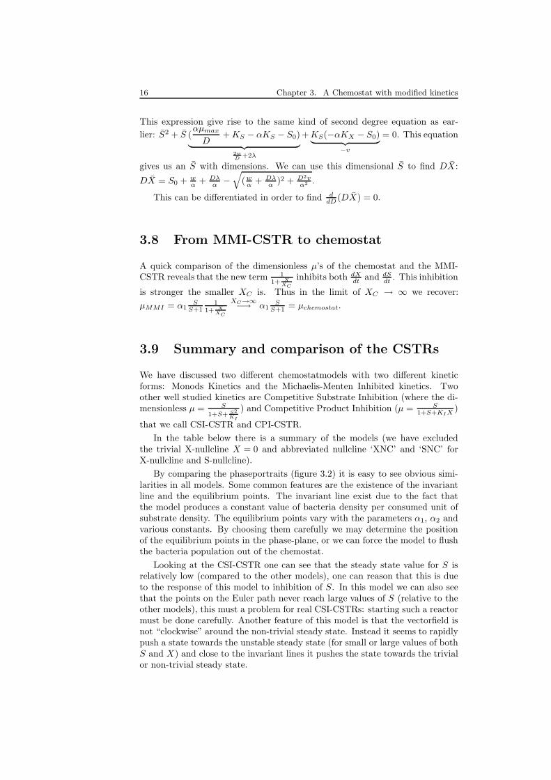
This expression give rise to the same kind of second degree equation as ear-

lier: S2 + S (αµmax

D+ KS − αKS − S0)

︸︷︷︸2wD

+2λ

+ KS(−αKX − S0)︸︷︷︸

−v

= 0. This equation

gives us an S with dimensions. We can use this dimensional S to find DX:

DX = S0 + wα + Dλ

α −

√

(wα + Dλ

α )2 + D2vα2 .

This can be differentiated in order to find ddD (DX) = 0.

3.8 From MMI-CSTR to chemostat

A quick comparison of the dimensionless µ’s of the chemostat and the MMI-CSTR reveals that the new term 1

1+ XXC

inhibits both dXdt and dS

dt . This inhibition

is stronger the smaller XC is. Thus in the limit of XC → ∞ we recover:

µMMI = α1S

S+11

1+ XXC

XC→∞−→ α1

SS+1 = µchemostat.

3.9 Summary and comparison of the CSTRs

We have discussed two different chemostatmodels with two different kineticforms: Monods Kinetics and the Michaelis-Menten Inhibited kinetics. Twoother well studied kinetics are Competitive Substrate Inhibition (where the di-mensionless µ = S

1+S+ S2

KI

) and Competitive Product Inhibition (µ = S1+S+KIX )

that we call CSI-CSTR and CPI-CSTR.

In the table below there is a summary of the models (we have excludedthe trivial X-nullcline X = 0 and abbreviated nullcline ‘XNC’ and ‘SNC’ forX-nullcline and S-nullcline).

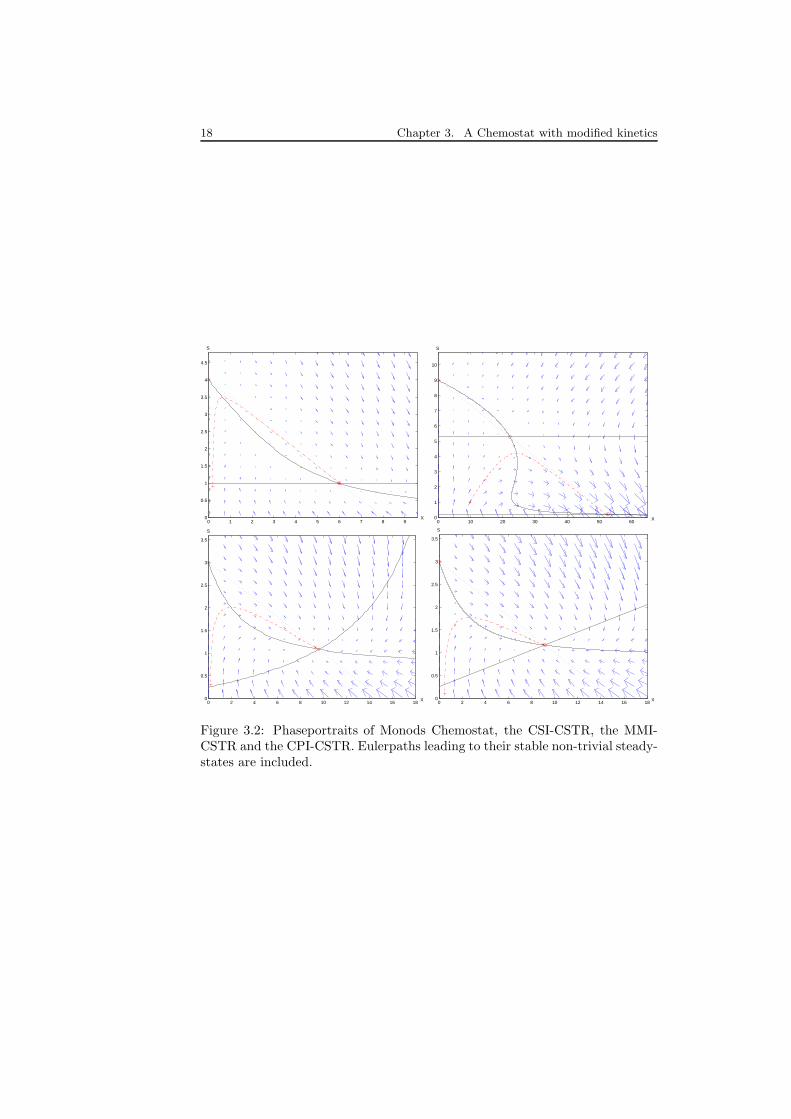
By comparing the phaseportraits (figure 3.2) it is easy to see obvious simi-larities in all models. Some common features are the existence of the invariantline and the equilibrium points. The invariant line exist due to the fact thatthe model produces a constant value of bacteria density per consumed unit ofsubstrate density. The equilibrium points vary with the parameters α1, α2 andvarious constants. By choosing them carefully we may determine the positionof the equilibrium points in the phase-plane, or we can force the model to flushthe bacteria population out of the chemostat.

Looking at the CSI-CSTR one can see that the steady state value for S isrelatively low (compared to the other models), one can reason that this is dueto the response of this model to inhibition of S. In this model we can also seethat the points on the Euler path never reach large values of S (relative to theother models), this must a problem for real CSI-CSTRs: starting such a reactormust be done carefully. Another feature of this model is that the vectorfield isnot “clockwise” around the non-trivial steady state. Instead it seems to rapidlypush a state towards the unstable steady state (for small or large values of bothS and X) and close to the invariant lines it pushes the state towards the trivialor non-trivial steady state.

3.9. Summary and comparison of the CSTRs 17

Model Monods Chemostat CSI-CSTR

µ S1+S

S

1+S+ S2

KI

dXdt α1

S1+S X − X α1

S

1+S+ S2

KI

X − X

dSdt − S

1+S X − S + α2 − S

1+S+ S2

KI

X − S + α2

XNC S = 1α1−1 S = KI(α1−1)

2 ±

√

(KI (α1−1)2 )

2− KI

SNC X = (α2−S)(1+S)S X =

(α2−S)(1+S+ S2

KI)

S

limit − KI → ∞

Model MMI-CSTR CPI-CSTR

µ S1+S

11+ X

XC

S1+S+KIX

dXdt α1

S1+S

X1+ X

XC

− X α1S

1+S+KIX X − X

dSdt − S

1+SX

1+ XXC

− S + α2 − S1+S+KIX X − S + α2

XNC S =1+ X

XC

α1−(1+ XXC

)S = XKI+1

α1−1

SNC X = (α2−S)(1+S)

S+ 1XC

(α2−S)(1+S)X = (α2−S)(1+S)

S−KI(α2−S)

limit XC → ∞ KI → 0

The other three models, the chemostat, the MMI-CSTR and the CPI-CSTRare quite similar in comparison to the CSI-CSTR. They have the similar null-clines and steady states in almost the same places and their vectorfields are alsosimilar. The chemostat S-nullcline is parallel to the X-axis and in two othermodels this nullcline increases with increasing values of X . This can be inter-preted as an inhibiting effect of X on µ: the vectorfield changes from pushinga state towards increasing X ’s to smaller X ’s when it crosses the S-nullcline(from large values of S). Monods chemostat does not “feel” this inhibition anddoes not care if the value of X is very large, it is S that determines if X shouldgrow or not.

The striking similarities of the MMI-CSTR and the CPI-CSTR are probablyan effect of their very similar µ’s, only the denominator differs.


0 1 2 3 4 5 6 7 8 90

0.5

1

1.5

2

2.5

3

3.5

4

4.5

X

S

0 10 20 30 40 50 600

1

2

3

4

5

6

7

8

9

10

X

S

0 2 4 6 8 10 12 14 16 180

0.5

1

1.5

2

2.5

3

3.5

X

S

0 2 4 6 8 10 12 14 16 180

0.5

1

1.5

2

2.5

3

3.5

X

S

Figure 3.2: Phaseportraits of Monods Chemostat, the CSI-CSTR, the MMI-CSTR and the CPI-CSTR. Eulerpaths leading to their stable non-trivial steady-states are included.

Chapter 4

Other CSTR-types

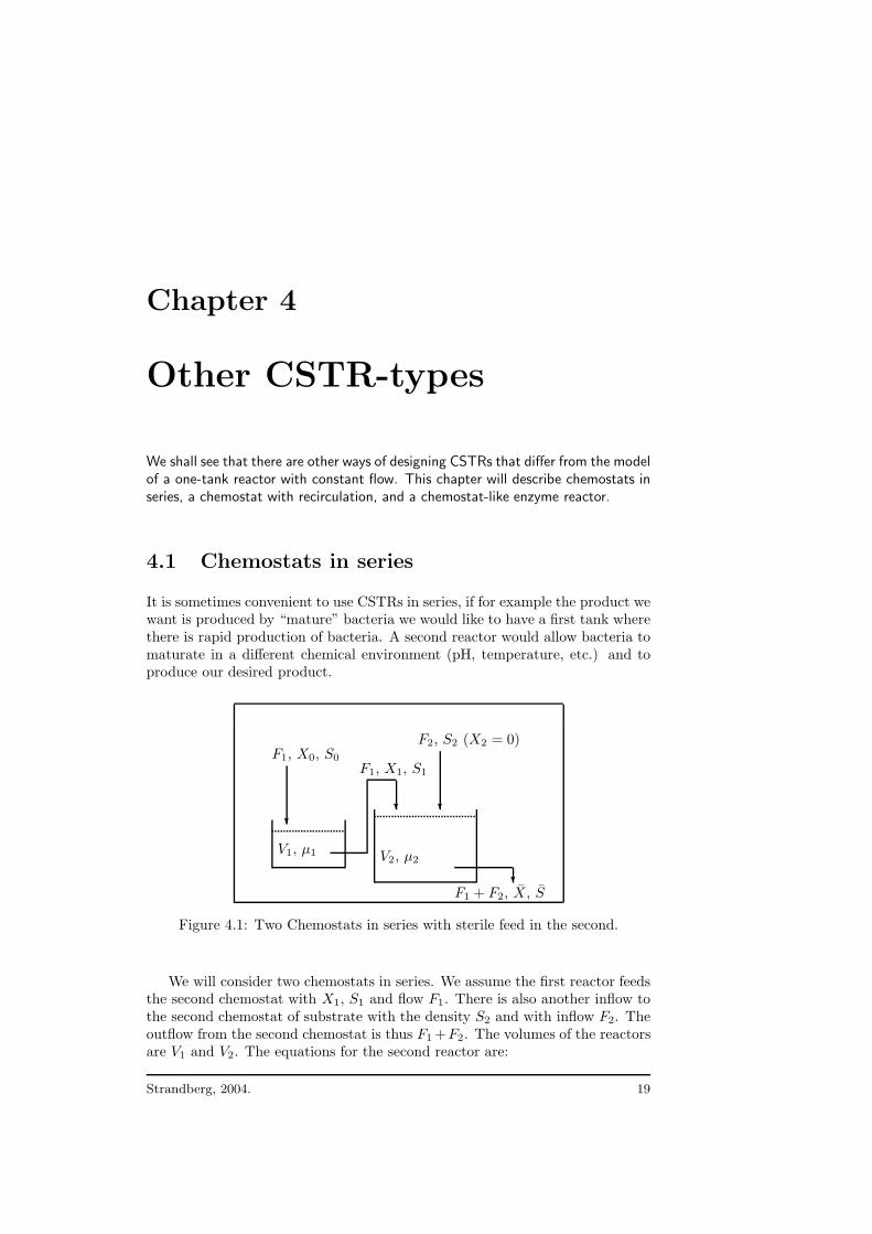
We shall see that there are other ways of designing CSTRs that differ from the modelof a one-tank reactor with constant flow. This chapter will describe chemostats inseries, a chemostat with recirculation, and a chemostat-like enzyme reactor.

4.1 Chemostats in series

It is sometimes convenient to use CSTRs in series, if for example the product wewant is produced by “mature” bacteria we would like to have a first tank wherethere is rapid production of bacteria. A second reactor would allow bacteria tomaturate in a different chemical environment (pH, temperature, etc.) and toproduce our desired product.

?

F1, X0, S0

?

F1, X1, S1

?

F2, S2 (X2 = 0)

?

F1 + F2, X, S

V1, µ1 V2, µ2

Figure 4.1: Two Chemostats in series with sterile feed in the second.

We will consider two chemostats in series. We assume the first reactor feedsthe second chemostat with X1, S1 and flow F1. There is also another inflow tothe second chemostat of substrate with the density S2 and with inflow F2. Theoutflow from the second chemostat is thus F1 +F2. The volumes of the reactorsare V1 and V2. The equations for the second reactor are:


20 Chapter 4. Other CSTR-types

dVdt = F1 + F2 − (F1 + F2) = 0

dXdt = F1

V1X1 + µX − F1+F2

V2X

dSdt = F1

V1S1 − αµX − F1+F2

V2S + F2

V2S2

(4.1)

We let D1 = F1

V1and D2 = F1+F2

V2⇔ F2

V2= D2−

F1

V2= D2−D1

V1

V2(> 0)

gives us the equations describing the equilibrium point in the second chemostat:

dXdt = D1X1 + µX − D2X = 0

dSdt = D1S1 + (D2 − D1

V1

V2)S2 − αµX − D2S = 0

We assume that µ 6= µ(X) for simplicity. We notice that there is only onesolution to the first equation: D1X1 + µX − D2X = 0 ⇔ X = D1X1

D2−µ .From the second relation and depending on the rate expression, we get dif-

ferent values of S and X.

4.2 Chemostat with recirculation

In some cases it is shown that recirculation of a fraction of the bacteria increasesthe productivity of the system.

?

F , S0

-

?

?

Separator

X1, S1

F (1 + ϕ)

F , (1 − c)X1, S 6= S1

ϕF , cX1, S = 0

Figure 4.2: The chemostat with recirculation.

Here we let the fraction ϕ of F recirculate back into the reactor. In thisfraction of medium (assumed to be without any S) we let the fraction c of Xbe reinserted into the system. The equations become:

dXdt = +cX · ϕD + µX − X(1 + ϕ)D

dSdt = −αµX − D(1 + ϕ)S + DS0

(4.2)

When searching for steady states we let X 6= 0 and from the first line in(4.2) we get dX

dt = 0 ⇔ µ = (1+ϕ−ϕc)D, now we notice that ϕ(1−c) > 0,since c is only a small fraction, and thus: µ > D, which is better that thereproduction we had in the earlier chemostats.

Again, different rate-expression give rise to different X and S. With Monodsµ we get: µ = µmaxS

KS+S = (1 + ϕ − ϕc)D The steady state is thus: (X, S) =(

S0−(1+ϕ)Sα(1+ϕ−ϕc) ,

KSD(1+ϕ−ϕc)µmax−D(1+ϕ−ϕc)

)

.

4.3. Chemostat-like enzyme reactors 21

4.3 Chemostat-like enzyme reactors

In this section we consider a CSTR with enzymes instead of bacteria.

If we make two fair assumptions: (1) one substrate molecule spawns oneproduct molecule giving S0 − S = P − P0 (thus “consumed substrate” = “pro-duced product”), and (2) the enzyme concentration (E) is constant (and equalto one) as time passes, we get the equations:

dEdt = 0 = 0

dSdt = D(S0 − S) − 1 · E · µ = D(S0 − S) − µ

dPdt = Eµ − DP = µ − DP

(4.3)

This is sufficient to find S if we first specify the kinetics. Let us use theMichaelis-Menten kinetics: µ = µmaxS

KS+S = D(S0 − S) ⇒

S =S0−KS−

µmaxD

2 ±

√

(S0−KS−

µmaxD

2 )2 + S0KS .

This is one way of finding the steady state S. It is however not alwayswhat we are interested in. If we use an alternative approach and introduce therelation δ = S0−S

S0, corresponding to the fraction of S0 that has been converted

into product. We notice S = S0(1 − δ) and we are able to search the dilutioncoefficient as a function of δ and S0 instead. This is often very convenient. Wewill now look at D’s for different kinetic cases.

Michaelis-Menten kinetics in an enzyme reactor

From (4.3) we get the relation D = µ(S0−S) and the Michaelis-Menten kinetics

is µ = µmaxSKS+S so we get: D = µ

S0−S = µmaxS(KS+S)(S0−S) = µmax(1−δ)

δ(KS+S0(1−δ)) .

Competitive Substrate Inhibition in an enzyme reactor

Now we apply Competitive Substrate Inhibition instead and in a similar waywe get: D = µ

S0−S = µmaxS

(S0−S)(KM+S+ S2

KI). Again using δ = S0−S

S0gives us:

D = µmax/δS0

1+KM

S0(1−δ)+

S0(1−δ)KI

.

Competitive Product Inhibition in an enzyme reactor

We remember the stochiometric relation S0−S = P−P0 ⇔ P = S0−S+P0,allowing us to eliminate P in µ.

By the same procedure as above and get:

D = µmaxS(S0−S)(KM (1+PKI)+S) =

1−δδ

µmax

KM+KM KI(δS0+P0)+S0(1−δ) .

Michaelis-Menten Inhibition in an enzyme reactor

This is actually not possible, since the kinetic expression contains X , a variablenot present in an enzyme reactor.

22 Chapter 4. Other CSTR-types

The dilutions rates summarised

Kinetics Kinetic expression Dilution coefficient

Michaelis-Menten µmaxSKS+S

µmax(1−δ)δ(KS+S0(1−δ))

CSI µmaxS

KM+S+ S2

KI

µmax/δS0

1+KM

S0(1−δ) +S0(1−δ)

KI

CPI µmaxSKM (1+PKI)+S

1−δδ

µmax

KM+KM KI(δS0+P0)+S0(1−δ)

Chapter 5

Controlled CSTRs and the

turbidostat

In this chapter we will discuss controlled CSTRs. By controlling a CSTR we willsee that the possibility to choose a steady state increases. Controlling a CSTR canalso be wise when the concentration of substrate in the inflow is fluctuating to limitfluctuations in the population density.

5.1 Controlled CSTRs

There are many ways to use automatic control in CSTRs to achieve good results.One general name for a class of controlled CSTR’s is auxostats. An auxostat isoften defined as a continuous culture system in which the concentration of oneof the components, for example the pH-level, biomass concentration, or nutri-tion concentration, is predetermined and the system is controlled to maintain aconstant level of this component.

One popular auxostat is the pH-auxostat since the active bacteria produceorganic acids as wasteproducts, lowering the pH. Measuring the pH is cheapand simple, and since pH is correlated to the productivity this type of auxostatis easy to control.

Another auxostat is the turbidostat. The turbidity of a solution that meanshow much light it absorbs is simple to measure, and is proportional to thedensity of biomass X in the vessel. If there is too much density more solutionis added, and vice versa.

In general we want to fix our X at a value XP, a point in the proximity ofthe uncontrolled systems steady state X0. By doing this we assume that thebehaviour of the system is the similar to its behaviour in the neighbourhood ofX0, even if this might be at some distance from X0.

A generalised controlled system can be described as:

ddtX = AX + BU, Y = CX, (5.1)

where U contain variables used to control the system and B is a constant matrix,for example the values from a linearization around the point of interest. Y isan output vector letting us observe values of X, and C describes how X and Y

are related. The dimension of the vector BU must be the same as for AX.


24 Chapter 5. Controlled CSTRs and the turbidostat

?

F (t), S0

?Lamp

⊗ ;

+/−Detector/

Controller

X(t), S(t)

?

F (t), X(t), S(t)

Figure 5.1: The general idea of the Turbidostat. Via a closed loop in thereactor light is passed through the solution. A detector/controller measures theturbidity and sends a signal to regulate the inflow of nutrient.

We will consider the case where U = X and the system is controlled byvarying D. We let D = D0 +D(X, S). Returning to (2.6) where D0 correspondsto our old D and with X0 = 0 we have:

dXdt = µX − D0X − D(X, S)XdSdt = −αµX − D0(S − S0) − D(X, S)(S − S0)

(5.2)

We will not yet describe D(X, S) in detail, but we will require two proper-ties. The first constraint is that we want D(XP) = 0, we do not want tochange anything if we are in the required state XP. The other constraint isD0 + D(X, S) ≥ 0, since we add positive volumes of the nutrition solution tothe CSTR.

We linearize (5.2) around X0: ddtX = AX + BX where:

A =

(µ′

XXP + µ − D0 µ′SXP

−αµ′XXP − αµ −αµ′

SXP − D0

)

B =

(−D′

XXP −D′SXP

D′X(S0 − SP ) D′

S(S0 − SP )

)

This expression can now be used to derive convenient forms of controlledCSTRs.

Two important questions about controlled systems is their controllabilityand stabilisability. A system that is controllable is also stabilisable. By control-lability we mean that a system, through a control policy, can be forced to movefrom an initial state Xi to a desired state Xd in finite time. Controllability inthis case is guaranteed when det[B AB . . . An−1B] 6= 0, and is not obtainedfor the turbidostat. This means that not all states can be obtained in finitetime.

Stabilisability is obtained when all eigenvalues of A can be made negativeby choosing a suitable control, but it may happen that eigenvalues of A arenegative from the beginning. This situation corresponds to our normal stabilitycondition when the trace is negative and the determinant is positive.

5.2. Invariant line for CSTRs controlled with D 25

5.2 Invariant line for CSTRs controlled with D

As for the uncontrolled systems we can examine ddt (S + αX). We end up with:

d

dt(S + αX) = −(S + αX − S0) (D0 + D(X, S))

︸︷︷︸

≥0

Thus if the equality αX = S0 − S is fulfilled, we tend to keep it fulfilled: theminus sign in this relation ensures that we return to the invariant line if we forsome reason were to move away from it.

So there is an invariant line for CSTRs controlled with D and it is the sameas for the uncontrolled CSTRs.

5.3 The turbidostat

We will now look at the case where D(X, S) = D(X) = KD(X − XP ). XP isthe value of X we want to stabilize our CSTR about. If we apply µ = µ(S), wehave µ′

X = 0. Also: D′S = 0 and D′

X = KD. The system is then:

dXdt = µX − D0X − KD(X − XP )XdSdt = −αµX − D0(S − S0) − KD(X − XP )(S − S0)

(5.3)

This expression can be analyzed to learn how the controller action acts in thiscase. If we search for a steady-state value of X we can ignore the trivial steadystate and end up with:

KDX = µ − D0 + KDXP ⇔

µ = D0, KD = 0

X = XP + µ−D0

KD, 0 < XP < ∞

X ≈ XP , KD ≫ µ − D0

KD is the key here: without control action (KD = 0) we return to Monodschemostat, for extremely large values of KD we end up with X = XP . Forreasonable values of KD we are close to XP . This middle expression also corre-sponds to a nullcline.

By linearizing (5.3) we get:

d

dtX = (A + B)X =

(µ − D0 − KDXP µ′

SXP

−αµ + KD(S0 − SP ) −αµ′SXP − D0

)

X

Now, sufficiently close to the steady state we can approximate D0 ≈ µ, allowingus to do some changes:

d

dtX ≈

(−KDXP µ′

SXP

−αµ + KD(S0 − SP ) −αµ′SXP − µ

)

X

As usual we want to know if this controlled system is stable and investigatethe trace and the determinant:

tr(A + B) = −KDXP − αµ′SXP − µ

If µ is strictly growing (and its derivative positive) then indeed tr(A + B) < 0.But if we for example have a CSI-CSTR µ′

S might be negative. A sufficientcondition is however KD > −αµ′

S .


If we assume that we are close to the invariant line and can use αXP ≈

S0 − SP , we get the determinant:

det(A + B) = µ′SKDXP (αXP − (S0 − SP ))

︸︷︷︸

≈0

+KDXP µ + XP µ(αµ′S + KD)

det(A + B) ≈ KDXP µ + XP µ(αµ′S + KD)

So we have a positive determinant if KD > −αµ′S , or if we have µ′

S > 0. Thissystem is thus stable. But since we do not have controllability we are not reallysure where we arrive to in the phase-plane.

5.4 The phaseportrait of a turbidostat

0 0.1 0.2 0.3 0.4 0.5 0.6 0.7 0.80

0.5

1

1.5

2

X

S

Figure 5.2: A phaseportrait of a Turbidostat. The diagonal dotted line is theinvariant line, the vertical dotted line corresponds to X = XP , the point-dottedline is an Euler path starting in (0.73, 2.2) and the full line an X-nullcline. Thering on the invariant line is where the steady state would have been withoutthe controller action. The arrows represent the vector-field composed of dX

dt anddSdt .

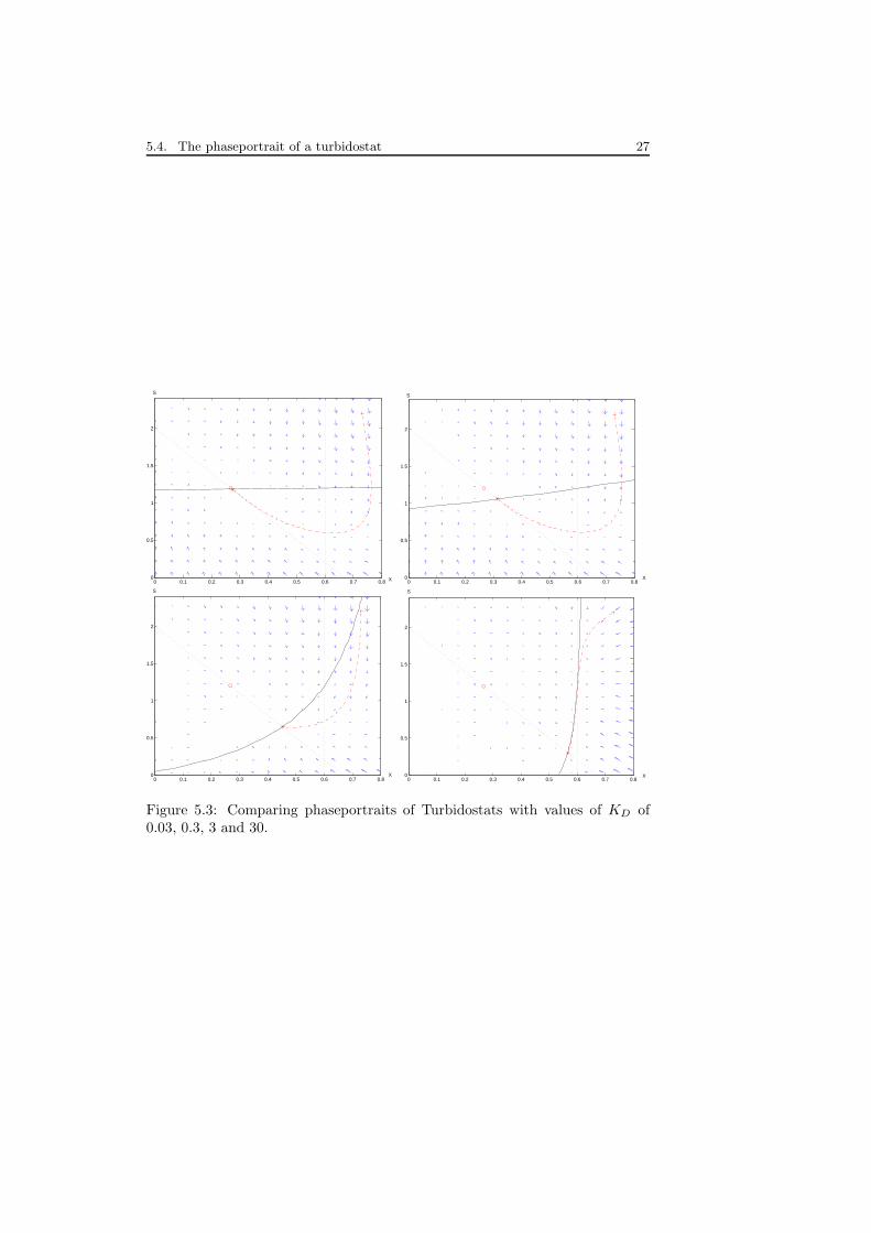
Looking at the phaseportrait of a Turbidostat, figure 5.2, the first strikingdifference is the distance between the normal chemostat steady state and thesteady state of the turbidostat. But here there is also an invariant line asbefore and a nullcline in about the same place as before. This nullcline dependshowever strongly on KD.

In figure 5.3 we see how the phase portrait changes with increasing valuesof KD: the nullcline tends to approach the line X = XP and thus the steadystate approaches the intersection of the null cline and of the invariant line.

5.4. The phaseportrait of a turbidostat 27

0 0.1 0.2 0.3 0.4 0.5 0.6 0.7 0.80

0.5

1

1.5

2

S

X 0 0.1 0.2 0.3 0.4 0.5 0.6 0.7 0.80

0.5

1

1.5

2

X

S

0 0.1 0.2 0.3 0.4 0.5 0.6 0.7 0.80

0.5

1

1.5

2

S

X 0 0.1 0.2 0.3 0.4 0.5 0.6 0.7 0.8

0

0.5

1

1.5

2

S

X

Figure 5.3: Comparing phaseportraits of Turbidostats with values of KD of0.03, 0.3, 3 and 30.

Chapter 6

Summary and conclusion

In this report several mathematical models of bacteria population growth inbioreactors were analyzed.

In chapter 2 we explored two simple models of biological growth: exponentialgrowth and by taking into account the substrate concentration, S, thelogistic equation. The exponential growth is typically seen when resourcesare good and the population is very small. The logistic equation explainshow a population is restricted by limited resources.

We introduced the in- and outflow of nutrient in our reactor, the Michaelis-Menten kinetics and analyzed Monods Chemostat. Equilibrium solutions,nullclines, the parameters α1 and α2 and the phaseportrait are found tobe useful characteristics.

Chapter 3 is dedicated to the new model proposed: the Michaelis-Menteninhibited CSTR. The MMI-CSTR exhibits different phaseportrait showinghow the MMI-CSTR responds to large values of X by inhibition.

A comparison of this model and Monods chemostat with the competitivesubstrate and product inhibition has been made.

In chapter 4 we discuss chemostats in series, a chemostat with recirculationand three chemostat-like enzyme reactors. We saw that in the chemostatwith recirculation we could achieve µ > D, and that chemostats in seriesallow us to take into account different ambient conditions for the bacteria.

In chapter 5 we have explained how a controlled CSTR works and investi-gated the turbidostat: it illustrates a simple way of controlling a CSTR.


30 Chapter 6. Summary and conclusion

Bibliography

[1] Leah Edelstein-Keshet, (1988), Mathematical Models in Biology, McGrawHill, Inc.

[2] Harvey W. Blanch, Douglas S. Clark, (1997), Biochemical Engineering,Marcel Dekker, New York.

[3] Carl-Fredrik Mandenius, (2002), Industriell Bioteknik, Bokakademin, Lin-koping.

[4] Colin Ratledge, Bjørn Kristiansen, (2001), Basic Biotechnology, CambridgeUniversity Press, Cambridge.

[5] Lennart Rade, Bertil Westergren, (2001), Mathematics Handbook for Sci-ence and Engineering (BETA), Studentlitteratur, Lund.

[6] Pramod Agrawal, Henry C. Lim, Analyses of various control schemes forContinuous bioreactors, Adv. Biochem. Eng, Biotech 30, (1984) 91-90.

[7] Steven P. Fraleigh, Henry R. Bungay, Lenore S. Clesceri, Continuous cul-ture, feedback control and auxostats, Tibtech, June 1989 [Vol. 7].

[8] Torkel Glad, Lennart Ljung, (1989), Reglerteknik grundlaggande teori, Stu-dentlitteratur, Lund.


32 Bibliography

Appendix A

The Linearized stability

A.1 The Linearization

F (x), a one-variable function of x can be Taylor-expanded around a fix X . Weget F (X + x) = F (X) + F ′(X)x + O(x2). For small perturbations of x aroundX we get the linearization: F (X + x) ≈ F (X) + F ′(X)x, containing only theconstant and the linear terms.

For functions of two variables F (X + x, S + s) and G(X + x, S + s):

F (X + x, S + s) = F (X, S) + F ′X(X, S)x + F ′

S(X, S)s + O((x + s)2)

G(X + x, S + s) = G(X, S) + G′X(X, S)x + G′

S(X, S)s + O((x + s)2)

If F (x, s) = dXdt , G(x, s) = dS

dt and the point (X, S) is an equilibrium point thenthe linearization is:

dXdt = F (X + x, S + s) ≈ F

′

X(X, S)x + F′

S(X, S)s = a11x + a12s

dSdt = G(X + x, S + s) ≈ G

′

X(X, S)x + G′

S(X, S)s = a21x + a22s

A convenient notation is ddtX ≈ AX =

(a11 a12

a21 a22

)

X, and is often used when

looking at the chemostat or other dynamical systems of similar mathematicalform.

A.2 The Stability

Now, let us use our linearization and look at some conditions needed for thelinearization to be stable. We have d

dtX = AX. Supposing that

x = c1 · v1eλ1t + c2 · v2eλ2t we get, for each λ: ddtX = λAeλt = Aveλt. Elim-

inating the exponential in the two last terms, we get the well-known equation:det(A − λI) = 0 that has two solutions:

λ =a11 + a22

2±

√

4(a12a21 − a11a22) + (a11 + a22)2

2⇔

λ =tr(A)

2±

√

−4det(A) + tr(A)2

2


34 Appendix A. The Linearized stability

In order to have stable solutions we must have Re(λ) < 0 and thus tr(A) < 0. Ifwe assume that tr(A) < 0 and look at the first λ (with a plus), we get λ1 < 0 ⇔

tr(A)

2+

√

−4det(A) + tr(A)2

2< 0 ⇔ 0 < det(A)

Thus, for us to not have a positive real part in our exponentials, we haveto have: tr(A) < 0 and det(A) > 0. This allows us to simply look at ourlinearization to know a lot of our how our system behaves near an equilibriumpoint.

Worth noting is also if the term

√

−4det(A) + tr(A)2

is real or complex. Ifa λ has a negative real part and no complex part in an equilibrium-point, thispoint could be considered to be a stable node because the exponentials includeonly negative real numbers.

If λ contains some complex parts we can easily discover that the pair of λ’smust be complex-conjugated and that the exponentials give rise of a spiral-likemotion in the (X,S)-plane around the equilibrium-point. We call the point astable spiral if tr(A) < 0.

Appendix B

A Matlab M-file

This appendix displays a Matlab M-file used to visualize the phase portrait and tocontrol calculations. This example explains the principle, and it is easy to change,for example, the kinetic expression to fit another model.

function chemostat_inhibited(alpha1, alpha2, xp0, sp0, xc)

%%chemostat_inhibited Displays a phaseportrait, nullclines% and an Euler-path of an inhibited Chemostat.

% chemostat_inhibited(alfa1, alfa2, np0, cp0, nc) will run if% alpha1 > 1/xc, thus there is a reproduction.

% alpha2 > 1/(xc*alpha1-1), thus there is sufficient stock-nutrition.% xp0 > 0 , you can not have a nonpositive population.% sp0 > 0 , you can not have a nonpositive concentration.

% xc > 0%

% The blue arrows represent the vectorfield.% The black lines are two of the three nullclines.

% The black dotted line is the invariant line (no solution crosses it).% The red line is an Eulerpath, starting in + and ending in *.%

% Try the following:% chemostat_inhibited(5, 3, 0.2, 0.3, 6)

%% by Per Erik Strandberg, 2003-2004.%

% Start-condition:

%------------------if ((alpha1>1) & (alpha2>0) & (sp0>0) & (xp0>0) & xc>0),

if (alpha2<1/(alpha1-1)),disp(’ ’)

disp (’ (HINT: Only the trivial steady state, alpha2 is too small...)’)else

disp(’ ’)disp (’ (HINT: Two steady states, alpha2 is quite large...)’)

end

% The non-trivial equilibrium-solution:%-----------------------------------------

a = (xc+1-alpha2-xc/alpha1);b = (-alpha2-xc/alpha1);sbar = -a/2 + sqrt(0.25*a*a-b) ;

xbar = -alpha1*sbar+alpha1*alpha2 ;

hold offplot(xbar, sbar, ’rO’)hold on

plot(0, alpha2, ’rO’)


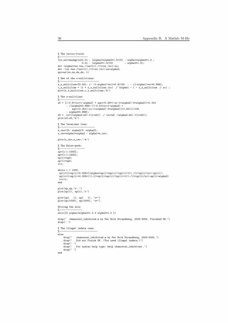
36 Appendix B. A Matlab M-file

% The vector-field:%--------------------

[xx,ss]=meshgrid(0.01 : (alpha1*alpha2*1.3/15) : alpha1*alpha2*1.3 ,0.01 : (alpha2*1.3/15) : alpha2*1.3);

dx= (alpha1*xx.*ss./(ss+1))./(1+xx./xc)-xx;ds= -(xx.*ss./(ss+1))./(1+xx./xc)-ss+alpha2;

quiver(xx,ss,dx,ds, 1)

% One of the x-nullclines:

%----------------------------x_x_nullcline=[0.001: (- (1-alpha1)*xc)*0.9/100 : - (1-alpha1)*xc*0.999];

c_x_nullcline = (1 + x_x_nullcline./xc) ./ (alpha1 - 1 - x_x_nullcline ./ xc) ;plot(x_x_nullcline,c_x_nullcline,’k’)

% The s-nullcline:%------------------

s5 = [(-0.5*(xc+1-alpha2) + sqrt(0.25*(-xc-1+alpha2)^2+alpha2))*1.001: ((alpha2*0.999)-((-0.5*(xc+1-alpha2) +

sqrt(0.25*(-xc-1+alpha2)^2+alpha2))*1.001))/100: alpha2*0.999];

x5 = xc*((alpha2-s5).*(1+s5)) ./ (xc*s5 -(alpha2-s5).*(1+s5));

plot(x5,s5,’k’)

% The Invariant line:%-------------------------s_inv=[0: alpha2/3 :alpha2];

x_inv=alpha1*alpha2 - alpha1*s_inv;

plot(x_inv,s_inv,’:k’)

% The Euler-path:%------------------xp=[1:1:1000];

sp=[1:1:1000];xp(1)=xp0;

sp(1)=sp0;i=1;

while i < 1000,xp(i+1)=xp(i)+0.005*((alpha1*xp(i)*sp(i)/(sp(i)+1))./(1+xp(i)/xc)-xp(i));

sp(i+1)=sp(i)+0.005*(((-1)*xp(i)*sp(i)/(sp(i)+1))./(1+xp(i)/xc)-sp(i)+alpha2)i=i+1;

end

plot(xp,sp,’r-.’)

plot(xp(1), sp(1),’r’)

plot(xp( 1), sp( 1), ’r+’)plot(xp(1000), sp(1000), ’r*’)

%fixing the axis%----------------

axis([0 alpha1*alpha2*1.2 0 alpha2*1.2 ])

disp(’ chemostat_inhibited.m by Per Erik Strandberg, 2003-2004. Finished OK.’)disp(’ ’)

% The illegal indata case:%---------------------------

elsedisp(’ chemostat_inhibited.m by Per Erik Strandberg, 2003-2004.’)disp(’ Did not Finish OK. (You used illegal indata.)’)

disp(’ ’)disp(’ For syntax help type: help chemostat_inhibited .’)

disp(’ ’)end

LINKÖPING UNIVERSITY

ELECTRONIC PRESS

Copyright

The publishers will keep this document online on the Internet - or its possi-ble replacement - for a period of 25 years from the date of publication barringexceptional circumstances. The online availability of the document implies apermanent permission for anyone to read, to download, to print out single copiesfor your own use and to use it unchanged for any non-commercial research andeducational purpose. Subsequent transfers of copyright cannot revoke this per-mission. All other uses of the document are conditional on the consent of thecopyright owner. The publisher has taken technical and administrative mea-sures to assure authenticity, security and accessibility. According to intellectualproperty law the author has the right to be mentioned when his/her work isaccessed as described above and to be protected against infringement. For ad-ditional information about the Linkoping University Electronic Press and itsprocedures for publication and for assurance of document integrity, please referto its WWW home page: http://www.ep.liu.se/

Upphovsratt

Detta dokument halls tillgangligt pa Internet - eller dess framtida ersattare- under 25 ar fran publiceringsdatum under forutsattning att inga extraordi-nara omstandigheter uppstar. Tillgang till dokumentet innebar tillstand forvar och en att lasa, ladda ner, skriva ut enstaka kopior for enskilt bruk ochatt anvanda det oforandrat for ickekommersiell forskning och for undervisning.Overforing av upphovsratten vid en senare tidpunkt kan inte upphava dettatillstand. All annan anvandning av dokumentet kraver upphovsmannens med-givande. For att garantera aktheten, sakerheten och tillgangligheten finns detlosningar av teknisk och administrativ art. Upphovsmannens ideella ratt in-nefattar ratt att bli namnd som upphovsman i den omfattning som god sedkraver vid anvandning av dokumentet pa ovan beskrivna satt samt skydd motatt dokumentet andras eller presenteras i sadan form eller i sadant sammanhangsom ar krankande for upphovsmannens litterara eller konstnarliga anseende elleregenart. For ytterligare information om Linkoping University Electronic Pressse forlagets hemsida http://www.ep.liu.se/

c© 2004, Per Erik Strandberg


lith - mai - ex - - 04 / 04 - - se - per erik strandberg - startsidan · ·...

Documents