stock returns and expected business conditions: half a
TRANSCRIPT

Stock Returns and Expected Business Conditions:
Half a Century of Direct Evidence
Sean D. Campbell Francis X. Diebold Federal Reserve Board University of Pennsylvania
and NBER
May 2005This Draft/Print: December 27, 2007
Abstract: Using half a century of Livingston survey data on expected business conditions, wecharacterize directly the impact of expected business conditions on expected excess stock returns. Expected business conditions consistently affect expected excess returns in a statistically andeconomically significant counter-cyclical fashion: Depressed expected business conditions areassociated with high expected excess returns. Moreover, inclusion of expected businessconditions in otherwise-standard predictive return regressions substantially reduces theexplanatory power of the conventional financial predictors, including the dividend yield, default
premium, and term premium, while simultaneously increasing . Expected business conditions
retain predictive power even after controlling for an important and recently introduced non-financial predictor, the generalized consumption/wealth ratio, which accords with the view thatexpected business conditions play a role in asset pricing different from and complementary to thatof the consumption/wealth ratio. We argue that time-varying expected business conditions likelycapture time-varying risk, while time-varying consumption/wealth may capture time-varying riskaversion.
Key Words: Business cycle, expected equity returns, prediction, Livingston survey, risk aversion,equity premium, risk premium
JEL Code: G12
Acknowledgments: For invaluable guidance we thank the Editor, the Associate Editor, and threereferees. For support we thank the Humboldt Foundation, the Guggenheim Foundation, theNational Science Foundation, and the Wharton Financial Institutions Center. For helpfulcomments we thank seminar participants at the Board of Governors of the Federal ReserveSystem and the Swiss National Bank (Study Center Gerzensee), as well as Andrew Ang, RaviBansal, Hui Guo, Martin Lettau, Sydney Ludvigson, Josh Rosenberg, Steve Sharpe, JessicaWachter, and Kamil Yilmaz. None of those thanked, however, are responsible for the outcome.

“... [if] cyclical variation in the market risk premium is present, ...we would expect to find
evidence of it from forecasting regressions of excess returns on macroeconomic variables
over business cycle horizons. Yet the most widely investigated predictive variables have
not been macroeconomic variables, but financial indicators.”
(Lettau and Ludvigson, 2005b)
1. Introduction
The relationship between equity returns and underlying macroeconomic fundamentals
presents a clear puzzle: Many have argued that expected business conditions should be linked to
expected excess returns (e.g., Fama and French, 1989, 1990; Chen, Roll and Ross, 1986; Barro,
1990), yet the standard predictors are not macroeconomic, but rather financial: Dividend yields,
default premia, and term premia. Several authors, including Campbell and Shiller (1988), Fama
and French (1988, 1989), Ferson and Harvey (1991), and Campbell (1991) have claimed that the
standard financial predictors may serve as proxies for expected business conditions, and they
interpret their predictive power through that lens. In the absence of direct expectations data,
however, the claim that expected excess equity returns are driven by expected business conditions
remains largely speculative.
Against this background, we use a well-known survey to provide direct evidence on the
links between expected business conditions and expected excess equity returns over some fifty
years. We ask two key sets of questions. First, are the standard financial predictors related to
expected business conditions, and if so, how?
Second, do expected business conditions indeed forecast future returns? Are expected
business conditions a useful predictor of excess returns even after controlling for the standard
financial predictors? And conversely, are the standard financial predictors useful even after
controlling for expected business conditions? If not, do any standard financial predictors retain
-2-
power after conditioning on expected business conditions?
We proceed as follows. In section 2 we describe the data, and in particular our survey-
based measure of expected business conditions. In section 3 we examine the links between
expected business conditions and the standard financial predictors. In section 4 we assess
whether expected business conditions have predictive content for excess returns, and we provide
many variations on the basic theme. In section 5, we interpret our results, and we conclude in
section 6.
2. Data
Here we introduce the data and document some of their properties. Unless noted
otherwise, all data are measured biannually. In Table 1 we report the name and a short
description of each series as well as its frequency, available sample range, mean, standard
deviation and first order autocorrelation coefficient.
Excess Stock Returns
We construct excess stock returns using the CRSP value-weighted portfolio and the 90-
day U.S. Treasury bill rate, 1952:1-2003:2.
Livingston Six-Month Growth Forecasts
The Livingston survey is widely followed, heavily studied, and generally respected, as
surveyed for example by Croushore (1997). Moreover, and importantly, it is available over a long
sample period, in contrast for example to the Survey of Professional Forecasters, which begins
only in 1968. The Livingston survey is biannual, conducted in June and December. Our sample
begins in 1952:1, which matches the beginning of the continuously-recorded Livingston survey
data, and continues until 2003:2. Note the notation associated with the bi-annual data: 2001:2,

-3-
for example, refers to the second half of 2001, i.e., 7/1/2001 through 12/31/2001.
We construct real GDP growth expectations from nominal GDP and CPI level expectations
reported in the Livingston survey, which solicits respondents’ views regarding economic variables
in six and twelve months’ time. Unfortunately, the Livingston survey does not ask participants
about expectations of current GDP or CPI levels, so we can not use it to construct one-step-ahead
forecasts (a step being a six-month interval). We aggregate the Livingston responses into median
forecasts, obtaining, for each series and survey date, a median forecast of the series’ level six and
twelve months hence, and we take log differences to obtain an approximate two-step-ahead
growth rate forecast, as in Gultekin (1983). The final result is a series of two-step-ahead real GDP
growth forecasts, , spanning 1952:1 - 2003:2.
The two-step-ahead real growth rate forecasts constructed from the Livingston data appear
well-behaved. In Figure 1 we show the actual growth rates, the Livingston forecasts, and the
corresponding forecast errors. The forecasts move with the actual growth rates but are smoother,
which is a well-known property of optimal forecasts of stationary series; see, for example, Diebold
(2004). Moreover, the forecast errors appear to have zero mean and display no obvious
predictable patterns. The sharp cutoff in the sample autocorrelation function of the forecast errors
beyond displacement one, as shown in Figure 2, indicates first-order moving average structure,
which is consistent with optimality of the two-step-ahead forecasts. The mean Livingston
(annualized) real GDP growth rate forecast in Table 1 is 2.54 percent, which closely accords with
historical growth realizations.
In Table 2, we examine the performance of the Livingston forecasts in more detail by
regressing realized real GDP growth, two steps ahead, on the Livingston forecasts as well as
-4-
lagged real GDP growth, real consumption growth, and real investment growth. The first column
of Table 2 indicates that the Livingston growth forecasts are informative about future real GDP
growth; the forecasts predict future growth with a t-statistic of 3.0. When compared to the
forecasting performance of lagged real GDP, consumption, and investment growth the Livingston
forecast stands out. Specifically, in each of the univariate specifications only the Livingston
forecast is a significant predictor of future GDP growth. Moreover, when the Livingston forecast
is combined with the other predictors the size and significance of the coefficient on the Livingston
forecast is unaffected. Accordingly, the Livingston forecast contains important information about
future real GDP growth which is not contained in other macroeconomic variables.
Financial Predictors
We examine several standard and widely-studied financial return predictors, the dividend
yield, , calculated for the CRSP value-weighted portfolio, the default premium, ,
calculated as the yield difference between a broad corporate bond portfolio and the Aaa yield, and
the term premium, , calculated as the yield difference between a ten-year Treasury bond
and a one-month Treasury bill, also 1952:1-2003:2. We also examined Santos and Veronesi’s
(2006) ratio of labor income to consumption and Bollerslev and Zhou’s (2006) variance risk
premium. Both of those variables, however, were consistently insignificant, so we omit them from
the results that follow.
Macroeconomic Predictors
We also examine two macroeconomic stock return predictors. The first is Lettau and
Ludvigson’s (2001a, b) consumption wealth ratio, . The second is a simple alternative to the
survey expectations of future expected real GDP growth. Specifically, we consider a forecast of

-5-
future real GDP growth, , based on lagged real GDP growth, consumption growth and
investment growth. We construct the forecast from the estimates in column (5) of Table 2. Each
of these macroeconomic predictors spans 1952:1 - 2003:2.
Additional Growth Forecasts
The Livingston six-month growth forecast, , is our primary measure of expected
future business conditions. We do, however, examine the robustness of our findings to other
measures of expected future business conditions. We now briefly describe these additional
expectations data.
Beginning in 1974, the December Livingston survey asks participants for their expectations
of nominal GDP and CPI levels in two years’ time. We use this data in conjunction with the
survey expectations for nominal GDP and the CPI levels in six months’ time to construct a
measure of expected real GDP growth over the eighteen month period beginning in six months’
time, . The data are annual and span the 1974-2003 period.
Beginning in 1991, the Livingston survey asks participants for their expectations of real
GDP growth over the next ten years. This long-term growth expectation, , is measured in
both the June and December survey and spans the 1991:1-2003:2 period.
The Survey of Professional Forecasters (SPF) is an alternative survey of expected business
conditions. It is a quarterly survey, which we aggregate to biannual for comparability with our
other analyses. It is unfortunately available only over a significantly shorter period than the
Livingston survey, but it also has some useful features that Livingston does not. Beginning in
1968, the SPF asks participants for their expectations for the level of real GDP in the current
period and in six months’ time. Because the SPF asks participants about their expectations for the

-6-
current level of real GDP (unlike the Livingston survey), we can construct one-step-ahead
forecasts for real GDP growth, , which span 1968:1-2003:2.
Beginning in 1968, the SPF asks participants for their expectations for the level of real
GDP in the current period and in twelve months’ time. We use these data to construct a measure
of expected real GDP growth over the following twelve months, , which spans 1968 -
2003.
Volatility Variables
We use data on the realized volatility of the CRSP value weighted daily return, ,
which is available 1963:1 - 2003:2, as well as data on the realized volatility of the S&P 500 daily
return, , which is available over the full sample period 1952:1 - 2003:2.
Additional Predictors and Macroeconomic Variables
We also use data on the growth rate of real GDP, , consumption, , and
investment, , from 1952:1 - 2003:2 to construct a macroeconomic factor that predicts real
GDP growth. We call that factor .
3. Relationships Among Expected Business Conditions, Financial Return Predictors and
Macroeconomic Return Predictors
In their classic assessment of the predictability of excess stock returns, Fama and French
(1989) find that excess returns are indeed predictable, with most predictive power coming from the
dividend yield, the default premium, and the term premium. More precisely, they estimate
regressions of the form
, (1)
and they document a strong relationship in terms of the usual t-statistics, values, and so forth,

-7-
where is the excess return on a broad stock portfolio over periods, for ranging from one
quarter to several years.
The Fama-French research program stresses the role that financial predictors play in
predicting stock returns. More recently, researchers have found evidence that macroeconomic
variables also may play a role in predicting stock returns. Lettau and Ludvigson (2001b), for
example, find that the ratio of consumption to wealth, , predicts stock returns.
The key open question is why financial and macroeconomic variables should predict excess
returns. In the case of the financial predictors, Fama and French (1989) suggest that the predictive
power may derive from their correlation with expected business (i.e., macroeconomic) conditions.
In the case of the macroeconomic predictors, it is also possible that at least part of their predictive
power stems from their information content about future real activity.
Notoriously little direct evidence exists, however, as to whether these financial and
macroeconomic variables actually are linked to expected business conditions. In this section we
provide precisely such direct evidence, examining the extent to which the Livingston real growth
expectations are linked to the standard financial and macroeconomic predictors, both pairwise and
jointly. We estimate regressions of Livingston expected business conditions on the
financial predictors ( , , ) and on as well as our macroeconomic data-based
measure of expected future real GDP growth, . In Table 3 we show results from both simple
and multiple regressions.
First consider the relationship between the financial predictors and the Livingston forecasts.
The simple regressions reveal some links between the financial variables and expected business
conditions, although the strength and statistical significance vary across variables and
-8-
specifications. First, the dividend yield is negatively, though insignificantly, related to expected
business conditions. This accords with the dividend discount model with a constant expected
return, which predicts that the dividend yield should fall when necessary to offset higher expected
growth in dividends. Second, the term premium is positively related to expected business
conditions. This accords with the basic notion that the yield curve slope is a leading indicator, with
inverted yield curves indicating a likely future recession, due for example to tightening of monetary
policy, which increases short rates. Finally, the default premium appears positively associated with
expected business conditions. This seemingly anomalous result may be due to the short horizons
associated with the Livingston forecasts; that is, notwithstanding the positive correlation between
default premia and expected business conditions at short horizons, default premia may be
negatively correlated with expected business conditions at longer horizons of, say, two or three
years.
The multiple regressions in Table 3 provide a summary distillation of the links between
expected real business conditions and the financial variables, taken jointly as a set. The results
show that expected business conditions are indeed systematically linked to the financial variables,
with s of roughly 25 percent. This is particularly noteworthy given the short horizons of the
Livingston expectations, because the dividend yield and term premium variables – in addition to
the default premium as already discussed – are often thought to have maximal predictive value at
much longer horizons.
Now consider the relationship between the macroeconomic variables and the Livingston
forecasts. The simple regressions show only a weak association between the Livingston forecasts
and each of the macroeconomic variables. In each case the estimated relationship is weak, with a

-9-
negative adjusted . The multiple regression results echo the simple regression results. Taken
together, the three macroeconomic variables only account for a small portion of the variation in the
Livingston forecasts. In this sense, the Livingston forecasts contain considerable information
regarding expectations about future business conditions over and above any that may be contained
in the macroeconomic variables. Hence the Livingston forecasts provide an excellent opportunity
to examine the role that expectations about future real activity play in predicting future stock
returns.
In summary, the results of this section help us to understand why the standard financial
variables “work” in predictive regressions for excess stock returns: They are correlated with
expected business conditions, as conjectured by Fama and French (1989). Crucially, however, the
correlation is far from perfect ( ). That is, the financial variables, even when taken jointly as
a set, provide only highly noisy proxies of expected business conditions. This suggests that, to the
extent that expected excess returns are driven by expected business conditions, superior return
predictions may be produced via a direct measure of expected business conditions. We now
provide precisely such a direct assessment of the effects of expected business conditions on
expected excess stock returns.
4. Expected Business Conditions and Expected Excess Returns
Thus far we have established that the standard financial predictors are indeed correlated
with expected business conditions. Now we go the full mile, asking whether expected business
conditions do indeed predict excess returns. We proceed in three steps. First, in section 4.1, we
focus on the predictive ability of the Livingston six-month growth forecasts, controlling for a
variety of other predictors. Second, in section 4.2, we retain focus on the Livingston six-month

-10-
forecasts, but we assess robustness to the return horizon, different sample periods, and different
timing conventions. Finally, in section 4.3, we explore other (non-Livingston) measures of
expected business conditions.
4.1 Main Results: Livingston Six-Month Growth Forecasts
We now consider the central question of whether and how expected business conditions are
linked to expected excess returns. We regress excess stock returns on the Livingston six-month
growth forecasts, , as well as additional financial and macroeconomic predictors,
, (2)
where the timing of the excess return matches that of expected business conditions
, and where we standardize all predictors to have zero mean and unit variance to facilitate
comparison of coefficient magnitudes.
Note that the predictive regression (2) involves a two-step-ahead forecast rather than the
one-step-ahead forecast commonly employed in the literature. We focus on two-step-ahead
forecasts for two reasons. First, there is some uncertainty as to the precise time when the growth
forecasts are made, because they are constructed from surveys, and some forecasts may in fact be
made after the end of June or December, resulting in an overlap in the information sets from which
and are derived. Focusing on forecasts of rather than guards against
this possibility. Second, and most importantly and obviously, pairing with
matches the timing of the excess return to the horizon of the growth forecast.
We show the results in Table 4. First consider the simple regressions in columns (1)-(6), in
which we include the various predictors one at a time, and consider in particular the results for the
Livingston six-month growth forecasts. The point estimate indicates an economically important

-11-
negative relationship between expected excess returns and expected business conditions, with a
one standard deviation decrease in producing roughly a 0.2 standard deviation increase
in expected excess returns. The relationship is highly statistically significant at any conventional
level, and the adjusted is quite high (for the return-prediction literature) at 3.80 percent.
The simple regression results for the standard financial predictors, , , and
, reported in columns (2)-(4), are comparatively lackluster. The coefficient point estimates
for the financial predictors are all smaller than that for ; indeed, those for , and
are less than half that of . Similarly, the significance levels for the conventional
predictors are weaker than that for , and and are statistically insignificant
at any conventional level. Finally, the adjusted values for the conventional predictors are all
smaller than that for , and those for and are negligible.
The simple regression results for the macroeconomic predictors, and , reported in
columns (5)-(6), show that is a strong predictor of excess returns, while is not. In the case
of the macroeconomic data-based forecast of future growth, , the point estimate is negative
which supports the notion that better expected future business conditions forecast lower excess
returns though the point estimate is small and insignificant.
Now consider the multiple regression results reported in columns (7)-(12) of Table 4.
Columns (7) and (8) show the effect of adding the Livingston six-month forecast to a regression of
excess stock returns on financial predictors. The point estimates in column (7) reveal that the
dividend yield is the strongest predictor among the financial predictors. Adding the Livingston
forecast, in column (8), reduces both the size of the dividend yield coefficient estimate and its t-
statistic by roughly one third, while simultaneously raising the adjusted by more than sixty
-12-
percent. Columns (9) and (10) show the effect of adding the Livingston forecast to a regression of
excess stock returns on macroeconomic predictors. The Livingston survey continues to have a
sizable and significant effect on future excess returns, nearly doubling the adjusted of the
forecast based solely on macroeconomic predictors. Columns (11) and (12) show the effect of
adding the Livingston forecast to a specification that includes both financial and macroeconomic
predictors. Even after controlling for both sets of predictors, the Livingston forecast has a large
and significant negative effect on future returns, resulting in roughly a fifty percent increase in the
adjusted of the forecast.
All told, the results in Table 4 clearly point to expected business conditions as a key
determinant of expected excess returns. Across each specification, we find that the Livingston
forecast is negatively related to future excess returns, and this effect is always significant at
standard significance levels. Moreover, the quantitative impact of expected future business
conditions is large. Only is estimated to have a larger effect on excess stock returns and
including the Livingston forecast always improves the adjusted of the multiple regression
specifications.
4.2 Variations I: Alternative Return Horizons, Sub-Sample Analysis, and Timing
The results thus far indicate that expected business conditions play a key role in forecasting
excess returns. Relative to other predictors employed in the literature, the forecasting power of
the Livingston six-month growth forecasts is large and significant. In this subsection we consider
three important extensions, assessing whether the results are stable across alternative return
horizons, sub-samples, and alternative return timing conventions.
Return Horizon

-13-
The results thus far provide clear evidence that expected business conditions help to
forecast excess returns at a six-month horizon. Now we examine the value of expected business
conditions in forecasting excess returns at various longer horizons. We measure the long-horizon
regression coefficients on the Livingston six-month growth forecast, , using Hodrick’s
(1992) unified vector autoregression (VAR) methodology, which produces predictive regression
coefficients and ’s at all horizons from a single underlying VAR.
In Table 5 we report long-horizon regression statistics for horizons ranging from six to
sixty months. As before, we standardize each predictor, so that we can compare the imputed long-
horizon regression coefficients across predictors. In the top and bottom panels of Table 5 we
present long-horizon multiple regression statistics implied by the Hodrick VAR system, excluding
and including expected business conditions, respectively. Each panel contains multiple regression
coefficients for each forecasting horizon and the implied .
The patterns in the multiple regression coefficients indicate that the effect of including
expected business conditions dissipates as the forecasting horizon lengthens. This is most evident
when comparing the effect of the dividend yield to that of expected business conditions. Inclusion
of expected business conditions reduces the dividend yield coefficient by roughly forty percent at
the six month horizon, whereas it reduces it by only 15 percent at the sixty month horizon. A
similar pattern arises for the long-horizon ’s. At the six month horizon, adding expected
business conditions to the set of predictors increases the by roughly 33 percent. At horizons
beyond 24 months, including expected business conditions produces only negligible changes in
return predictability.
The general pattern in coefficients and predictability at horizons beyond six months

-14-
indicates that expected business conditions are most useful for predicting excess returns over the
six to 24 month horizon. This finding is appealing. It is consistent with both the short to medium
term nature of the Livingston forecasts, and with the possibility that other predictors contain
information, not contained in the Livingston forecasts, of relevance for forecasting longer-term
excess returns. Quite naturally, then, the information content of the Livingston forecasts appears
most relevant over the horizons to which they are tailored. Recently the Livingston survey has
added forecasts of longer-run growth (eighteen months and ten years ahead), which we
subsequently examine.
Sub-Samples
Although the full sample results presented in Table 4 indicate that expected business
conditions have a strong and negative effect on future excess returns, it is worth considering
whether or not this finding is robust across sub-samples. Hence we break the full sample into two
equal periods: 1952:1 - 1977:2 and 1978:1 - 2003:2. In Table 6, we report estimates of the most
important specifications from Table 4 over the two sub-samples.
Columns (1)-(3) and (8)-(10) show estimates of the simple regressions over the two sub-
samples for the three most important predictors of excess returns identified in Table 4, ,
, and . The predictive contents of the Livingston forecast, , and the
consumption-wealth ratio, , are relatively stable over the two sub-samples. In each case, the
point estimates vary within a relatively narrow range and exhibit similar degrees of statistical
significance across both sub-samples. In contrast, the predictive content of the dividend yield,
, varies considerably across the two sub-samples. In the early sub-sample the dividend yield
strongly predicts future excess returns, both in terms of its estimated effect and statistical

-15-
significance. In the late sub-sample the point estimate is considerably smaller (0.08 vs. 0.52) and
insignificant. Moreover, the adjusted over the late sub-sample is actually negative.
Columns (4)-(5) and (11)-(12) compare the effect of adding the Livingston six-month
growth forecast to a multiple regression that only employs financial predictors. In both sub-
samples, adding the Livingston forecast to the financial predictors results in a negative point
estimate, although the point estimate in the early sub-sample is smaller in magnitude and
statistically insignificant. In the early sub-sample the large and significant effect of the dividend
yield tends to crowd out the Livingston forecast. Columns (6)-(7) and (13)-(14) compare the
effect of adding the Livingston forecast to a multiple regression that only employs macroeconomic
predictors. Across both sub-samples the Livingston forecast has a sizeable negative effect on
future excess returns that is similar to the simple regression point estimate from each sub-sample.
All told, the results of the sub-sample analysis in Table 6 indicate that the effect of the
Livingston six-month forecasts on future excess returns is relatively stable. In the case of the
simple regressions, the point estimates are negative, of similar magnitude (-0.2 and -0.3), and of
similar statistical significance across both periods. In the case of the multiple regressions, higher
growth forecasts are associated with lower future excess returns in every specification. Although
the dividend yield crowds out much of the effect of the Livingston forecasts in the early sub-
sample, this should be tempered by the fact that the effect of the dividend yield is unstable across
the different sub-samples.
Return Timing
Thus far we have presented evidence that expected business conditions forecast excess
returns based on variants of equation (2), , in which we

-16-
regress two-step-ahead excess returns on the Livingston six-month forecasts and other predictors.
Although we have argued that this is the most appropriate timing convention given the timing of
the survey and the horizon of the growth forecasts, it is worthwhile to examine whether the
predictive content of the Livingston forecasts is sensitive to this timing convention. We do this by
estimating the following regression,
, (3)
which uses the one-step-ahead excess return, , rather than the two-step-ahead excess return,
, as the dependent variable. We report the results in Table 7. The specifications that we
examine in Table 7 are identical to those in Table 4.
The point estimate on the Livingston forecasts in the simple regression, reported in column
(1), is -0.17, which is significant at the one percent level though reduced somewhat relative to the
result in Table 4 (-0.22). Looking across each of the simple regression specifications in columns
(1)-(6) of Table 7 shows that the results are similar to those reported in Table 4. In particular,
both and are identified as significant predictors of excess returns in the simple
regressions, with point estimates that are similar in size and significance to those reported in Table
4. One important difference between these results and those reported in Table 4 is that, over the
one-step-ahead horizon, the forecasting power of dominates that of the Livingston forecasts
and all of the other predictors that we examine. Over this horizon and this sample period the
forecasting power of is quite remarkable, while the forecasting power of the Livingston
forecasts is more in line with that reported earlier.
All told, the simple and multiple regression results reported in Table 7 indicate that the
effect of the Livingston forecasts on future excess returns is robust to differences in the precise

-17-
timing of excess returns. In particular, across all specifications we find that the point estimate is
negative, similar in magnitude to that reported in Table 4, and statistically significant at the ten
percent level or better in three out of four cases. Moreover, in every case, adding the Livingston
six-month forecast improves the adjusted of the regression, further suggesting that expected
business conditions are an important determinant of excess stock returns.
4.3 Variations II: Additional Measures of Expected Business Conditions
The six-month Livingston growth forecast, , is our primary measure of expected
business conditions due to its long sample period, 1952:1-2003:2, and biannual frequency. These
survey forecasts, however, are not the only available measures of expected real GDP growth. In
this section we examine the robustness of our results to additional measures of expected business
conditions. Specifically, we use two additional measures of expected future real GDP growth from
the Livingston survey as well as two measures of expected future real GDP growth from the
Survey of Professional Forecasters (SPF). Each of these additional measures is available over a
different and shorter sample and in some cases at a lower frequency than the Livingston six-month
growth forecasts. As a result, the statistical precision of the results that follow is naturally weaker
than that of the Livingston six-month growth forecasts. Also, because additional forecasts all have
differing sample ranges and frequencies, the precise timing and frequency of the following
regressions depends on the specific forecast and control variables employed.
In Table 8 we examine the relationship between excess stock returns and two additional
real GDP growth forecasts from the Livingston survey as well as two real GDP growth forecasts
from the SPF. We run each regression in Table 8 using a set of non-overlapping observations as in
Tables 4-7. We also specify each regression to make the horizon of the excess return close to the
-18-
horizon of the corresponding growth forecast wherever possible. Finally, to avoid unnecessary
distraction, we show only point estimates and standard errors for the estimated coefficients on the
additional growth forecasts, using a “C” to denote that a predictor has been controlled for in the
regression.
The first additional growth forecast that we examine in Table 8 is the Livingston survey’s
annual (December) forecast of growth over the 18 month period beginning in 6 months’ time,
. This forecast provides a slightly longer term view of the macroeconomy than the six-
month forecast, , but it is only available at the annual frequency, and only since 1974.
Given its annual frequency, we regress annual excess returns on the lagged value of the forecast,
. We consider two specifications, reported in columns (1) and (5).
In a simple regression of excess returns on this forecast we find a negative relationship between the
forecast and future excess returns that is similar in size to the estimate reported for the Livingston
six-month growth forecast in Tables 4, 6, and 7. The point estimate, -0.19, however, is statistically
insignificant at standard levels. When we control for the financial and macroeconomic predictors
in column (5), the point estimate is still negative, and its magnitude increases to -0.38 and is
significant at the 5 percent level.
Next we consider the Livingston forecast of real GDP growth over the next ten years
following each survey (June and December), . This forecast provides for a long-term view
of the macroeconomy and is biannual but is only available since 1991:1. In this case we simply
regress our biannual excess returns on the lagged value of the forecast,
, because matching the horizon of the excess return with that of
the forecasts is impractical over the available sample. The results, reported in columns (2) and (6),
-19-
are also supportive of a negative relationship between expected business conditions and excess
returns. In each specification, the point estimate is negative, large in magnitude, and statistically
significant.
We now consider the growth forecasts from the SPF. The first forecast that we examine is
the SPF forecast of real GDP growth over the six month period immediately following the survey,
, which is closest in spirit to the Livingston six-month forecasts. The main drawback to the
SPF forecast is its short sample period, 1968:1 - 2003:2, relative to the Livingston six-month
forecasts. In the case of , we regress the one-step-ahead growth forecast on one-step
ahead biannual excess returns, . We report the results in columns
(3) and (7). In each specification we find a negative though insignificant relationship. We also
consider the SPF forecast of annual real GDP growth as well, . In this case we regress
annual excess returns on the lagged SPF forecast, . We report the
results in columns (4) and (8). In both cases we find that the estimates are not statistically
significant at standard levels.
Looking across the range of point estimates presented in Table 8 indicates that additional
measures of expected future business conditions are also negatively related to future excess
returns. Although the size and significance of the point estimates vary, the overall pattern is clear.
In 7 of 8 specifications we find a negative relationship between survey-based forecasts of future
business conditions and excess returns. Although the general pattern in the results is clear, it is
important to note that the statistical significance of the results reported in Table 8 are weaker than
those reported for the six-month Livingston forecasts in Tables 4, 6, and 8. Two points regarding
the statistical significance of the results are worth considering. First, the additional forecasts that

-20-
we examine in Table 7 are available only over a shorter sample period than that of the Livingston
six-month forecasts. Second, the measures of statistical significance that we report are marginal
rather than joint and thus do not account for the breadth and consistency of the results across the
entire set of additional forecasts.
5. Discussion
We have documented a robust negative correlation between expected excess returns and
expected business conditions, so that, for example, low expected future growth is associated with
high current expected excess stock returns. Here we address an important issue: Why the
negative relationship? Our answer is two-fold.
First, the high persistence of real activity over the business cycle should contribute to a
negative relationship. In particular, business cycle regimes (especially expansions) typically last for
much longer than six to twelve months, so the rational forecast is “good times now, likely good
times in the future,” and conversely. Hamilton’s (1989) classic Markov-switching analysis, for
example, produces one-step (quarterly) “staying probabilities” of =0.9 for expansions and
=0.75 for contractions. Iterating forward we obtain two-quarter staying probabilities of
=0.84 for expansions and =0.59 for contractions. Hence, over the horizons of one or two
quarters of most relevance for our analysis, current conditions are more likely to persist than to
reverse. The Livingston expectations rationally reflect that fact, rendering them positively rather
than negatively correlated with current conditions, and hence negatively related to expected excess
returns. This contrasts with – but in no way contradicts – the fact emphasized in the recent finance
literature that over very long horizons current conditions are likely to mean-revert.
Second, expected business conditions may forecast future volatility and hence may be

-21-
linked to perceived systematic risk and expected excess returns. The claim that business conditions
are linked to stock market volatility is certainly not new. In particular, as persuasively documented
in an extensive study by Schwert (1989) and echoed in subsequent work by Hamilton and Lin
(1996) using very different and complementary methods, stock market risk increases in recessions.
Indeed, in our view real activity is the only important and robust covariate of stock market
volatility thus far identified, notwithstanding the many investigations.
In Table 9 we examine the link between expected business conditions and realized stock
market volatility. We use two data sources to compute realized biannual stock return volatility.
The first is the daily CRSP value-weighted index, which is available since 1963, resulting in a
sample from 1963:1 through 2003:2. The second is the daily S&P 500 index, which is available
since 1951, resulting in a sample from 1951:2 through 2003:2. Then we regress realized volatility,
, on expected business conditions, , and the other predictors considered earlier as
well as a lag of realized volatility, . As in Table 8, we show only the point estimates and
standard errors on expected business conditions to avoid distraction, using “C” to denote that a
predictor has been controlled for.
Consider first the regression results for CRSP-based realized volatility in columns (1)-(7).
The results indicate that expected business conditions have highly statistically significant predictive
ability for volatility. The estimated relationship between expected business conditions and future
volatility agrees with the findings of previous research: Low growth expectations forecast high
stock return volatility. Moreover, even after controlling for lagged volatility as well as other
financial and macroeconomic predictors, expected business conditions emerge as a highly
significant predictor of volatility, with a t-statistic in excess of 2.0 across each of the seven

-22-
specifications. As in the univariate case, low growth expectations presage high future volatility.
Now consider the results for S&P-based realized volatility in columns (8)-(14) of Table 9.
The sign of the univariate coefficient estimate matches that of the CRSP-based estimate in column
(1), although the magnitude of the univariate estimate is smaller for the longer S&P-based sample.
The multiple regression results, however, are more uniform across the two samples. In particular,
the estimated coefficient for expected business conditions changes only slightly from -0.51 in the
top CRSP-based panel to -0.32 in the S&P-based panel once we control for lagged volatility as
well as the financial and macroeconomic predictors, and the t-statistic exceeds 2.5 in both cases.
Accordingly, both the CRSP and S&P based volatility measures indicate a negative and statistically
significant relationship between expected future business conditions and stock market volatility.
It is worth asking whether the full-sample relationship between expected business
conditions and stock market volatility documented in Table 9 is robust to sub-sample analysis. In
Table 10 we report selected specifications from Table 9 over the 1952-1977 sub-sample (columns
1-6) and the 1978-2003 sub-sample (columns 7-12). We report results for both the CRSP and
S&P 500 volatility measures.
The early sub-sample results indicate a negative relationship between expected future
business conditions and future stock market volatility in 4 of 6 specifications. The results in the
case of the CRSP volatility measure are stronger than for the S&P 500 volatility results. In
particular, although sets of point estimates are typically insignificant, the size of the effect of
expected future business conditions stock market volatility is typically an order of magnitude larger
in the CRSP volatility data than in the S&P 500 data.
The late sub-sample results also indicate that expectations of better economic performance

-23-
forecast lower stock return volatility. Unlike the early sub-sample, however, both the estimated
size of the relationship and the degree of statistical significance are similar across both the CRSP
and S&P 500 volatility measures.
All told, there is substantial evidence that expected business conditions have robust
predictive ability for volatility. Although the degree of statistical significance is reduced in each of
the sub-samples, the sign and size of the relationship is largely stable.
6. Concluding Remarks
Our key result, of course, is that expected business conditions are a robust predictor of
excess returns. An interesting secondary result is that the Lettau-Ludvigson (2001a, b) generalized
consumption / wealth ratio (CAY) is also a robust predictor, in contrast to other predictors that
feature prominently in the literature but often “drop out” once expected business conditions and
CAY are included. Presumably the time-variation in expected excess returns is ultimately driven
by time-varying expected risk and/or time-varying risk aversion. Hence the question naturally
arises as to whether and how expected business conditions and CAY are linked to equity market
risk and risk aversion.
We believe that the Livingston business conditions expectations likely capture time-varying
risk, as we discussed in detail in Section 5. But what of the Lettau-Ludvigson generalized
consumption/wealth ratio, ? We believe that likely captures time-varying risk aversion,
via the following logical chain:
(1) Theoretically, time-variation in expected excess returns is ultimately driven by time-
varying expected risk, time-varying risk aversion, or both;
(2) Empirically, time-variation in expected excess returns is driven by two key predictors,

-24-
expected business conditions and ;
(3) Expected business conditions are linked to risk;
(4) Expected business conditions and are largely unrelated;
(5) Hence, by elimination, must be linked to risk aversion.
Our assertion that captures time-varying risk aversion matches that of Lettau and Ludvigson
(2001b) and provides a largely independent confirmation of their work, insofar as we arrive at the
insight via a very different route. Note, however, that we do not assert that movements in
are exclusively driven by movements in risk aversion. In particular, our volatility forecasting
results indicate that movements in are also related to movements in risk.
Interestingly, Lettau and Ludvigson (2002, 2005a) document that forecasts future
investment and cash flows (dividends and earnings). Their findings, however, indicate that the
forecasting power of CAY for those variables is concentrated at relatively long horizons, in contrast
to the short/medium horizons associated with our expected business conditions variable.
Accordingly, we conjecture that measures both risk aversion and a risk component unrelated
to the risk component forecast by the Livingston expectations.
Both our results and our interpretation are very much in agreement with an emerging
empirical view that expected excess returns are counter-cyclical – not only for stocks, as in Lettau
and Ludvigson (2001b), but also for bonds, as in Cochrane and Piazzesi (2005) and Ludvigson and
Ng (2007). Interestingly, part of the literature emphasizes higher risk in recessions, as in
Constantinides and Duffie (1996), and another part emphasizes higher risk aversion in recessions,
as in Campbell and Cochrane (1999). Our results unify those two literatures, suggesting that the
cyclicality of both risk and risk aversion contributes to the counter-cyclicality of expected excess

-25-
returns: Growth expectations are procyclical and have a robust negative impact on expected
excess returns, and CAY is countercyclical and simultaneously has a robust positive impact.
References
Andersen, T.G., Bollerslev, T., Diebold, F.X. and Wu, J. (2005), “A Framework for Exploring theMacroeconomic Determinants of Systematic Risk,” American Economic Review, 95(May), 398-404.
Barro, R.J. (1990), “The Stock Market and Investment,” Review of Financial Studies, 3, 115-131.
Bollerslev, T. and Zhou, H. (2006), “Expected Stock Returns and Variance Risk Premia,” Financeand Economics Discussion Series, 2007-11, Board of Governors of the Federal ReserveSystem.
Campbell, J.Y. (1991), “A Variance Decomposition for Stock Returns,” Economic Journal, 101,157-179.
Campbell, J.Y. and Cochrane, J.H. (1999), “By Force of Habit: A Consumption-BasedExplanation of Aggregate Stock Market Behavior,” Journal of Political Economy, 107,205-251.
Campbell, J.Y. and Shiller, R.J. (1988), “The Dividend-Price Ratio and Expectations of FutureDividends and Discount Factors,” Review of Financial Studies, 1, 195-227.
Chen, N.-F., Roll, R. And Ross, S.A. (1986), “Economic Forces and the Stock Market,” Journalof Business, 56, 383-403.
Christoffersen, P.F. and Diebold, F.X. (1997), “Optimal Prediction Under Asymmetric Loss,”Econometric Theory, 13, 808-817.
Cochrane, J.M. and Piazzesi, M. (2005), “Bond Risk Premia,” American Economic Review, 95,138-160.
Constantinides, G.M. and Duffie, D. (1996), “Asset Pricing with Heterogeneous Consumers,”Journal of Political Economy, 104, 219-240.
Croushore, D. (1997), “The Livingston Survey: Still Useful After All these Years,” BusinessReview, Federal Reserve Bank of Philadelphia, March, 15-27.
Diebold, F.X. (2004), Elements of Forecasting, third edition. Cincinnati: South-Western.
Fama, E. and French, K. (1988), “Dividend Yields and Expected Stock Returns,” Journal ofFinancial Economics, 19, 3-29.
Fama, E. and French, K. (1989), “Business Conditions and Expected Returns on Stocks andBonds,” Journal of Financial Economics, 25, 23-49.
Fama, E. and French, K. (1990), “Stock Returns, Expected Returns, and Real Activity,” Journal

of Finance, 45, 1089-1108.
Ferson, W.E. and Harvey, C.R. (1991), “The Variation of Economic Risk Premiums, ” Journal ofPolitical Economy, 99, 1393-1413.
Gultekin, N. B. (1983), “Stock Market Returns and Inflation Forecasts,” Journal of Finance, 38,663-673.
Hamilton, J.D. (1989), “A New Approach to the Economic Analysis of Nonstationary Time Seriesand the Business Cycle,” Econometrica, 57, 357-84.
Hamilton, J.D. and Lin, G. (1996), “Stock Market Volatility and the Business Cycle,” Journal ofApplied Econometrics, 11, 573-593.
Hodrick, R. (1992), “Dividend Yields and Expected Stock Returns: Alternative Procedures forInference and Measurement,” Review of Financial Studies, 5, 357-386.
Leitch, G. and Tanner, J.E. (1991), “Economic Forecast Evaluation: Profits Versus theConventional Error Measures,” American Economic Review, 81, 580-90.
Lettau, M. and Ludvigson, S. (2001a), “Resurrecting the Consumption CAPM: A Cross-SectionalTest When Risk Premia Are Time-Varying,” Journal of Political Economy, 109, 1238-1287.
Lettau, M. and Ludvigson, S. (2001b), “Consumption, Aggregate Wealth, and Expected StockReturns,” Journal of Finance, 56, 815-849.
Lettau, M. and Ludvigson, S. (2002), “Time-Varying Risk Premia and the Cost of Capital: AnAlternative Implication of the q Theory of Investment,” Journal of Monetary Economics,49, 31-66.
Lettau, M. and Ludvigson, S. (2005a), “Expected Returns and Expected Dividend Growth,”Journal of Financial Economics, 76, 583-626.
Lettau, M. and Ludvigson, S. (2005b), “Measuring and Modeling Variation in the Risk-ReturnTradeoff,” in Y. Ait-Sahalia and L.P Hansen (eds.), Handbook of Financial Econometrics. Amsterdam: North-Holland, forthcoming.
Ludvigson, S. and Ng., S. (2006), “Macro Factors in Bond risk Premia,” Manuscript, New YorkUniversity and University of Michigan.
Santos, T. and Veronesi, P. (2006), “Labor Income and Predictable Stock Returns,” Review ofFinancial Studies, 19, 1-44.
Schwert, G.W. (1989), “Why Does Stock Market Volatility Change Over Time?,” Journal ofFinance, 44, 1115-1153.

Table 1Variable Descriptions and Descriptive Statistics
Variable Description Sample Frequency
Excess Stock Return
six-month return on the CRSP value weighted index net of
the return on a 90 day T-bill, reported as annualized
percentage
1951:2 -2003:2
semi-annual 6.51 15.74 -0.02
Livingston Six-Month Growth Forecasts
expected six-month growth rate in real GDP between the end
of period t+1 and t+2 computed from the median Livingston
survey response concerning the level of nominal GDP and
the CPI at the end of period t+1 and t+2, reported as
annualized percentage
1951:2 -2003:2
semi-annual 2.54 1.07 0.73
Financial Predictors
dividend yield on the CRSP value-weighted portfolio,
reported as annualized percentage1951:2 -2003:2
semi-annual 3.37 1.07 0.88
the yield spread between a broad corporate bond portfolio
and the Aaa yield spread, reported as annualized percentage1951:2 -2003:2
semi-annual 0.96 0.43 0.85
the yield spread between a 10 year U.S. Treasury bond and a
1 month Treasury bill, reported as annualized percentage1951:2 -2003:2
semi-annual 0.79 1.02 0.66
Macroeconomic Predictors
Lettau and Ludvigson (2001) log consumption-wealth ratio 1951:2 -2003:2
semi-annual 0.00 0.01 0.72
Macroeconomic factor used for forecasting two-step ahead
real GDP growth1951:2 -2003:2
semi-annual 3.24 0.35 -0.07
Additional Growth Forecasts
annualized expected eighteen-month growth rate in real GDP
between the end of period t+1 and t+4 computed from the
median Livingston survey response concerning the level of
nominal GDP and the CPI at the end of period t+1 and t+4,
reported as annualized percentage
1974 -2003
annual 2.61 1.11 0.74
expected 10 year real GDP growth rate computed from the
median Livingston survey response concerning real GDP
growth over the next ten years, reported as annualized
percentage
1991:1 -2003:2
semi-annual 2.75 0.38 0.85
annualized expected six-month growth rate in real GDP
between the end of period t and t+1 computed from the
median SPF survey response concerning the level of real
GDP at the end of period t and t+1, reported as annualized
percentage
1968:2 -2003:2
semi-annual 2.64 1.84 0.54
expected annual growth rate in real GDP between the end of
period t and t+2 computed from the median SPF survey
response concerning the level of real GDP at the end of
period t and t+2, reported as annualized percentage
1968-2003
annual 2.60 1.65 0.25
Volatility Measures
Realized volatility of the CRSP value-weighted return,
reported as annualized percentage1963:1 -2003:2
semi-annual 12.97 5.71 0.53
Realized volatility of the S&P 500 return, reported as
annualized percentage1951:2 -2003:2
semi-annual 13.18 5.78 0.49

Additional Predictors and Macroeconomic Variables
six-month growth rate in real GDP between the end of period
t and t+1, reported as annualized percentage 1951:2 -2003:2
semi-annual 3.24 2.12 0.28
six-month growth rate in real consumption between the end
of period t and t+1, reported as annualized percentage
1951:2 -2003:2
semi-annual 2.02 1.07 0.35
six-month growth rate in real investment between the end of
period t and t+1, reported as annualized percentage
1951:1 -2003:2
semi-annual 3.99 10.17 0.14
Notes: We report the notation and description of each variable in the first and second column. The sample range of eachvariable is reported in the third column. The frequency of each series is reported in the fourth column. The sample mean,standard deviation and first-order autocorrelation coefficient of each variable is reported in the fourth, fifth and sixthcolumn.

Table 2The Predictive Content of the Livingston
Six-Month Growth Forecasts
(1) (2) (3) (4) (5) (6)
0.24(0.08)
-- -- -- -- 0.25(0.08)
-- -0.07(0.11)
-- -- -0.19(0.27)
-0.19(0.15)
-- -- 0.09(0.22)
-- 0.33(0.33)
0.29(0.32)
-- -- -- -0.02(0.02)
0.00(0.04)
0.00(0.04)
4.91 -0.46 -0.81 0.00 -0.78 4.86
Wald 0.00 0.46 0.66 0.35 0.57 0.00
Notes: We report OLS estimates of regressions of real GDP growth, , onto the Livingston six-month growth
forecasts and several other macro predictors, 1952:1-2003:2, with Newey-West robust standard errors in parentheses. We
also report the adjusted , ,as well as the p-value of the Wald test that none of the included variables forecast future
real GDP growth in the final two rows of the table.

Table 3Regressions of Livingston Six-Month Growth Forecasts on Financial and Macro
Predictors
(1) (2) (3) (4) (5) (6) (7) (8)
-0.22(0.21)
-- -- -- -- -0.34(0.17)
-- -0.34(0.22)
-- 0.40(0.13)
-- -- -- 0.49(0.13)
-- 0.50(0.14)
-- -- 0.20(0.09)
-- -- 0.07(0.09)
-- 0.09(0.12)
-- -- -- -0.10(0.10)
-- -- -0.10(0.10)
-0.07(0.13)
-- -- -- -- -0.02(0.09)
-- -0.03(0.09)
-0.07(0.08)
3.94 15.38 3.12 -0.04 -0.01 26.32 -1.01 26.14
Wald 0.27 0.00 0.03 0.33 0.84 0.00 0.59 0.00
Notes: We report OLS estimates of regressions of real GDP growth expectations, , on several predictors, 1952:1-
2003:2, with Newey-West robust standard errors in parentheses. We also report the adjusted , , as well as the p-
value of the Wald test that none of the included variables are related to the Livingston forecasts in the final two rows of thetable. We standardize all variables. See text for details.

Table 4 Regressions of Excess Stock Returns on Six-Month Growth Forecasts, Financial Predictors and Macro Predictors
(1) (2) (3) (4) (5) (6) (7) (8) (9) (10) (11) (12)
-0.22(0.08)
-- -- -- -- -- -- -0.21(0.09)
-- -0.20(0.09)
-- -0.20(0.10)
-- 0.19(0.10)
-- -- -- -- 0.25(0.10)
0.17(0.10)
-- -- 0.19(0.12)
0.12(0.11)
-- -- -0.02(0.08)
-- -- -- -0.11(0.07)
-0.01(0.09)
-- -- -0.10(0.08)
0.00(0.09)
-- -- -- 0.10(0.08)
-- -- 0.15(0.07)
0.17(0.07)
-- -- 0.09(0.09)
0.11(0.09)
-- -- -- -- 0.24(0.07)
-- -- -- 0.24(0.08)
0.22(0.08)
0.17(0.11)
0.15(0.10)
-- -- -- -- -- -0.03(0.07)
-- -- -0.01(0.06)
-0.02(0.06)
-0.01(0.06)
-0.03(0.07)
3.80 2.67 -1.00 -0.03 4.96 -0.88 3.43 5.71 3.97 6.92 3.85 5.78
Wald 0.01 0.04 0.80 0.20 0.00 0.64 0.04 0.00 0.00 0.00 0.01 0.00
Notes: We report OLS estimates of regressions of excess returns, , on various predictors, 1952:1-2003:2, with Newey-West robust standard errors in
parentheses. We report the adjusted , , as well as the p-value of the Wald test that none of the included variables forecast future excess returns in the final
two rows of the table. We standardize all variables. See text for details.

Table 5 Long-Horizon Regressions of Excess Stock Returns on
Six-Month Growth Forecasts, Financial Predictors and Macro Predictors
Forecasting Horizon (Months)
Multiple Regression Long-Horizon Betas, Excluding
0.19 0.36 0.52 0.67 0.81 0.94 1.05 1.16 1.27 1.36
-0.10 -0.18 -0.25 -0.31 -0.36 -0.40 -0.45 -0.40 -0.52 -0.55
0.09 0.15 0.19 0.22 0.24 0.25 0.26 0.27 0.27 0.28
0.17 0.29 0.39 0.45 0.50 0.53 0.54 0.55 0.55 0.55
-0.01 -0.03 -0.04 -0.06 -0.07 -0.08 -0.08 -0.09 -0.10 -0.10
7.64 11.32 13.02 13.69 13.84 13.71 13.45 13.12 12.76 12.41
Multiple Regression Long-Horizon Betas, Including
-0.20 -0.32 -0.38 -0.41 -0.42 -0.42 -0.40 -0.39 -0.37 -0.35
0.12 0.25 0.38 0.51 0.64 0.75 0.86 0.96 1.05 1.14
0.00 -0.04 -0.11 -0.18 -0.25 -0.32 -0.38 -0.44 -0.49 -0.53
0.11 0.19 0.25 0.29 0.33 0.36 0.38 0.40 0.42 0.43
0.15 0.26 0.34 0.39 0.43 0.46 0.48 0.50 0.50 0.51
-0.03 -0.05 -0.07 -0.08 -0.08 -0.09 -0.10 -0.10 -0.11 -0.11
10.18 13.69 14.72 14.77 14.44 13.97 13.45 12.93 12.42 11.95
Notes: We report long-horizon regression coefficients and values for horizons ranging from six to sixty months,
1952:1-2003:2. In the top panel we report multiple regression coefficients and values for a specification that excludes
Livingston six-month growth forecasts as a predictor. In the bottom panel we report coefficients and values for a
specification that includes the Livingston forecast as a predictor. We standardize all predictors. See text for details.

Table 6Regressions of Excess Stock Returns on Six-Month Growth Forecasts, Financial Predictors and Macro Predictors: Sub-Sample Analysis
(1) (2) (3) (4) (5) (6) (7) (8) (9) (10) (11) (12) (13) (14)
1952-1977 1978-2003
-0.18(0.11)
-- -- -0.01(0.25)
-- -0.16(0.13)
-0.33(0.14)
-- -- -- -0.46(0.20)
-- -0.32(0.14)
-- 0.52(0.21)
-- 0.53(0.22)
0.52(0.25)
-- -- -- 0.08(0.11)
-- 0.23(0.12)
0.17(0.09)
-- --
-- -- -- 0.01(0.14)
0.02(0.26)
-- -- -- -- -- -0.21(0.14)
-0.01(0.07)
-- --
-- -- -- -0.04(0.19)
-0.03(0.23
-- -- -- -- 0.13(0.09)
0.20(0.08)
-- --
-- -- 0.31(0.16)
-- -- 0.31(0.16)
0.29(0.16)
-- -- 0.20(0.07)
-- -- 0.19(0.07)
0.17(0.06)
-- -- -- -- -- -0.01(0.08)
-0.01(0.08)
-- -- -- -- -- -0.07(0.11)
-0.07(0.10)
2.25 9.88 4.22 6.09 4.05 2.03 3.38 4.64 -0.82 4.25 1.87 7.67 2.71 6.62
Wald 0.08 0.01 0.05 0.11 0.14 0.14 0.15 0.02 0.44 0.01 0.15 0.01 0.03 0.02
Notes: We report OLS estimates of regressions of excess returns, , on various predictors with Newey-West robust standard errors in parentheses over two
sub-samples: 1952-1977 and 1978-2003. We report the adjusted , , as well as the p-value of the Wald test that none of the included variables forecast
future excess returns in the final two rows of the table. We standardize all variables. See text for details.
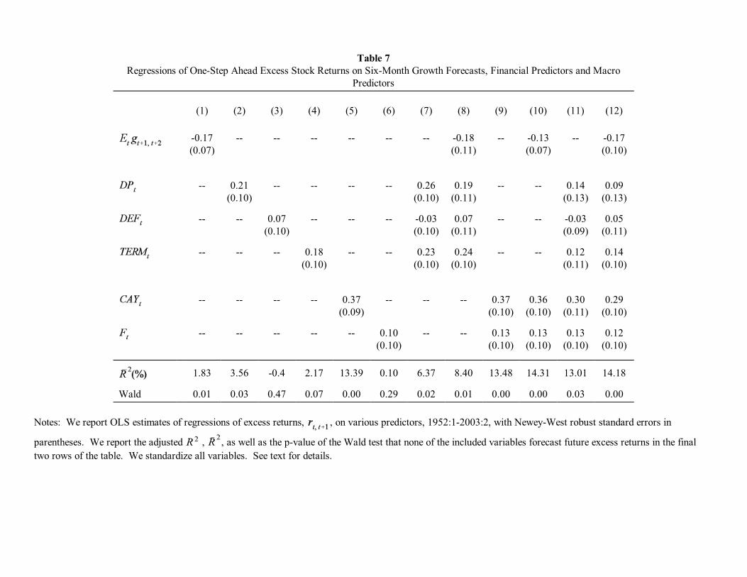
Table 7Regressions of One-Step Ahead Excess Stock Returns on Six-Month Growth Forecasts, Financial Predictors and Macro
Predictors
(1) (2) (3) (4) (5) (6) (7) (8) (9) (10) (11) (12)
-0.17(0.07)
-- -- -- -- -- -- -0.18(0.11)
-- -0.13(0.07)
-- -0.17(0.10)
-- 0.21(0.10)
-- -- -- -- 0.26(0.10)
0.19(0.11)
-- -- 0.14(0.13)
0.09(0.13)
-- -- 0.07(0.10)
-- -- -- -0.03(0.10)
0.07(0.11)
-- -- -0.03(0.09)
0.05(0.11)
-- -- -- 0.18(0.10)
-- -- 0.23(0.10)
0.24(0.10)
-- -- 0.12(0.11)
0.14(0.10)
-- -- -- -- 0.37(0.09)
-- -- -- 0.37(0.10)
0.36(0.10)
0.30(0.11)
0.29(0.10)
-- -- -- -- -- 0.10(0.10)
-- -- 0.13(0.10)
0.13(0.10)
0.13(0.10)
0.12(0.10)
1.83 3.56 -0.4 2.17 13.39 0.10 6.37 8.40 13.48 14.31 13.01 14.18
Wald 0.01 0.03 0.47 0.07 0.00 0.29 0.02 0.01 0.00 0.00 0.03 0.00
Notes: We report OLS estimates of regressions of excess returns, , on various predictors, 1952:1-2003:2, with Newey-West robust standard errors in
parentheses. We report the adjusted , , as well as the p-value of the Wald test that none of the included variables forecast future excess returns in the final
two rows of the table. We standardize all variables. See text for details.

Table 8Regressions of Excess Stock Returns on Alternative Growth Forecasts, Financial Predictors and Macro Predictors
Sample Range (1) (2) (3) (4) (5) (6) (7) (8)
1974-2003 -0.19(0.13)
-- -- - -0.38(0.18)
-- -- --
1991:1-2003:2 -- -0.36(0.17)
-- -- -- -0.28(0.15)
-- --
1968:1-2003:2 -- -- -0.08(0.10)
-- -- -- -0.04(0.11)
--
1968-2003 -- -- -- -0.07(0.13)
-- -- -- 0.10(0.21)
FinancialPredictors
1952:1 - 2003:2 -- -- -- -- C C C C
MacroPredictors
1952:1 - 2003:2 -- -- -- -- C C C C
1.64 20.57 -0.94 -2.53 16.85 23.65 8.20 28.02
Wald 0.14 0.04 0.44 0.69 0.00 0.06 0.74 0.64
Notes: We report OLS estimates of regressions of excess returns on alternative growth forecasts, a set of financial predictors, , and a set of
macro predictors, , with Newey-West standard errors in parentheses. We use a “C” to denote that a set of variables has been controlled for in the
regression. The sample range and frequency of each variable is reported in the second column. The range and frequency of each regression is determined by the
shortest sample and lowest frequency of all the included variables. We report the adjusted , , as well as the p-value of the Wald test that the corresponding
growth forecast does not forecast future excess returns in the final two rows of the table. We standardize all variables. See text for details.
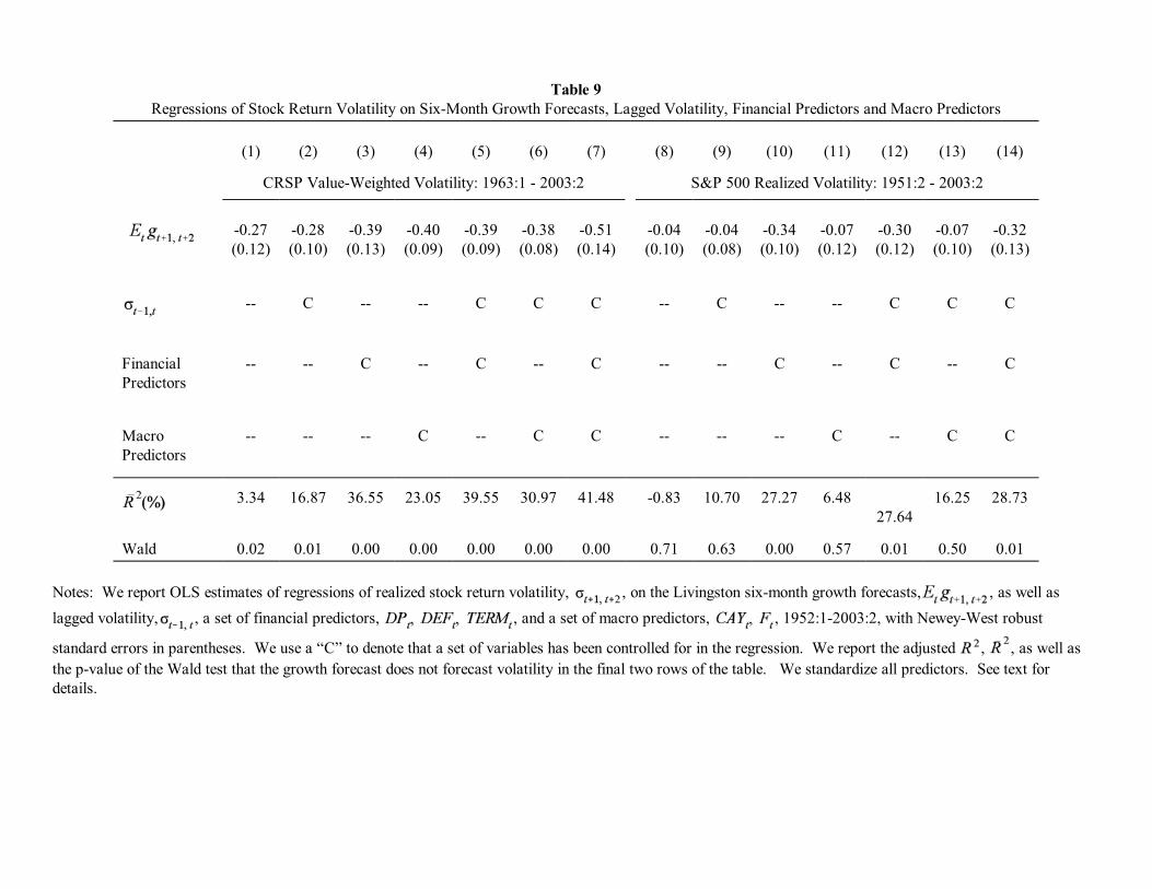
Table 9Regressions of Stock Return Volatility on Six-Month Growth Forecasts, Lagged Volatility, Financial Predictors and Macro Predictors
(1) (2) (3) (4) (5) (6) (7) (8) (9) (10) (11) (12) (13) (14)
CRSP Value-Weighted Volatility: 1963:1 - 2003:2 S&P 500 Realized Volatility: 1951:2 - 2003:2
-0.27(0.12)
-0.28(0.10)
-0.39(0.13)
-0.40(0.09)
-0.39(0.09)
-0.38(0.08)
-0.51(0.14)
-0.04(0.10)
-0.04(0.08)
-0.34(0.10)
-0.07(0.12)
-0.30(0.12)
-0.07(0.10)
-0.32(0.13)
-- C -- -- C C C -- C -- -- C C C
FinancialPredictors
-- -- C -- C -- C -- -- C -- C -- C
Macro Predictors
-- -- -- C -- C C -- -- -- C -- C C
3.34 16.87 36.55 23.05 39.55 30.97 41.48 -0.83 10.70 27.27 6.4827.64
16.25 28.73
Wald 0.02 0.01 0.00 0.00 0.00 0.00 0.00 0.71 0.63 0.00 0.57 0.01 0.50 0.01
Notes: We report OLS estimates of regressions of realized stock return volatility, , on the Livingston six-month growth forecasts, , as well as
lagged volatility, , a set of financial predictors, , and a set of macro predictors, , 1952:1-2003:2, with Newey-West robust
standard errors in parentheses. We use a “C” to denote that a set of variables has been controlled for in the regression. We report the adjusted , , as well as
the p-value of the Wald test that the growth forecast does not forecast volatility in the final two rows of the table. We standardize all predictors. See text fordetails.

Table 10 Regressions of Stock Return Volatility on Six-Month Growth Forecasts, Lagged Volatility, Financial Predictors and Macro
Predictors: Sub-Samples
(1) (2) (3) (4) (5) (6) (7) (8) (9) (10) (11) (12)
1952 - 1977 1978 - 2003
CRSP S&P 500 CRSP S&P 500
-0.25(0.15)
-0.15(0.18)
-0.26(0.14)
0.01(0.05)
-0.03(0.77)
0.00(0.06)
-0.19(0.17)
-0.35(0.33)
-0.19(0.12)
-0.16(0.16)
-0.47(0.38)
-0.18(0.14)
C C C C C C C C C C C C
FinancialPredictors
-- C -- -- C -- -- C -- -- C --
Macro Predictors
-- -- C -- -- C -- -- C -- -- C
10.78 24.75 24.07 2.85 1.63 3.38 5.40 29.72 37.51 3.36 22.95 25.30
Wald 0.10 0.43 0.05 0.78 0.77 0.97 0.27 0.29 0.12 0.34 0.22 0.21
Notes: We report OLS estimates of regressions of realized stock return volatility, , on the Livingston six-month growth forecasts, , as well as
lagged volatility, , a set of financial predictors, , and a set of macro predictors, , with Newey-West robust standard errors in
parentheses over two sub-samples: 1952-1977 and 1978-2003. We use a “C” to denote that a set of variables has been controlled for in the regression. We report
the adjusted , , as well as the p-value of the Wald test that the corresponding growth forecast does not forecast volatility in the final two rows of the table.
We standardize all predictors. See text for details.

Figure 1Real GDP Growth, Livingston Forecast, and Livingston Forecast Error
Notes: On the right scale we show U.S. bi-annual real GDP and the corresponding Livingstonforecast. On the left scale we show the their difference, the forecast error. See text for details.

Figure 2Sample Autocorrelation Function
Two-Step Ahead Real GDP Growth Forecast Errors
Notes: We report the sample autocorrelation function of two-step-ahead Livingston real GDPgrowth forecast errors, 1952:1-2003:2, along with approximate ninety-five percent confidenceintervals under the null hypothesis of white noise. The forecasts are made bi-annually, so theautocorrelation displacement is measured in units of six months. Hence, for example, adisplacement of two corresponds to one year. The Ljung-Box statistic for testing the hypothesis ofzero autocorrelations at displacements 2 through 25 is 18.76, which is insignificant at anyconventional level. See text for details.