Expected Returns and Expected Growth in Rents

of Commercial Real Estate∗

Alberto Plazzi † Walter Torous ‡ Rossen Valkanov §

This Version: January 2010 ¶

Abstract

Commercial real estate expected returns and expected rent growth rates are time-

varying. Relying on transactions data from a cross-section of U.S. metropolitan areas,we find that up to 30% of the variability of realized returns to commercial real estate

can be accounted for by expected return variability, while expected rent growth ratevariability explains up to 45% of the variability of realized rent growth rates. The cap

rate, that is, the rent-price ratio in commercial real estate, captures fluctuations inexpected returns for apartments, retail, as well as industrial properties. For offices, by

contrast, cap rates do not forecast (in-sample) returns even though expected returnson offices are also time-varying. As implied by the present value relation, cap rates

marginally forecast office rent growth but not rent growth of apartments, retail andindustrial properties. We link these differences in in-sample predictability to differencesin the stochastic properties of the underlying commercial real estate data generating

processes. Also, rent growth predictability is mostly observed in locations characterizedby higher population density and stringent land use restrictions. The opposite is true for

return predictability. The dynamic portfolio implications of time-varying commercialreal estate returns are also explored in the context of a portfolio manager investing in

the aggregate stock market, Treasury bills as well as commercial real estate.

∗We thank Andrea Berardi, Markus Brunnermeier (AFA discussant), Christopher Downing, Erasmo Giambona(EFA discussant), Harrison Hong, Andrey Pavlov, Antonio Rubia, Stephen Schaefer and seminar participants at thefollowing conferences for useful comments: the AFA 2007 Meeting, the AREUEA, the XXXIV EFA Meeting, theXXXVI EWGFM, the FMA European meeting, the SAET meeting in Vigo, and the SAFE center at the Universityof Verona. We are especially grateful to an anonymous referee and the Editor, Matthew Spiegel, for many suggestionsthat have greatly improved the paper. All remaining errors are our own.

†The Anderson School at UCLA and SAFE Center University of Verona, 110 Westwood Plaza, Los Angeles, CA90095-1481, phone: (310) 825-8160, fax: (310) 206-5455, e-mail: alberto.plazzi.2010@anderson.ucla.edu.

‡The Anderson School at UCLA, 110 Westwood Plaza, Los Angeles, CA 90095-1481, phone: (310) 825-4059, fax:(310) 206-5455, e-mail: walter.n.torous@anderson.ucla.edu.

§Corresponding author. Rady School at UCSD, Pepper Canyon Hall, 9500 Gilman Drive, MC 0093, La Jolla, CA92093, phone: (858) 534-0898, fax: (858) 534-0745, e-mail: rvalkanov@ucsd.edu.

¶The latest draft is available at: http://www.rady.ucsd.edu/valkanov

1 Introduction

U.S. commercial real estate prices fluctuate considerably, both cross-sectionally as well as over time.

For example, the return to apartment buildings during the last quarter of 1994 ranged from 21.4

percent in Dallas, Texas to −8.5 percent in Portland, Oregon. Eight years later, during the last

quarter of 2002, the returns to apartments in Dallas and Portland were 1.2 percent and 4.4 percent,

respectively. Other types of commercial real estate, such as retail, industrial, and office properties,

have experienced even larger return fluctuations. Understanding what drives these fluctuations is

an important research question as commercial real estate represents a substantial fraction of total

U.S. wealth. For example, Standard and Poor’s estimates the value in 2007 of all U.S. commercial

real estate to be about $5.3 trillion, about one fifth of the stock market’s value.

From an asset pricing perspective, the price of a commercial property, be it an office building,

apartment, retail or industrial space, equals the present value of its future rents. This fundamental

present value relation implies that observed fluctuations in commercial real estate prices should

reflect variation in future rents, or in future discount rates, or both. The possibility of time-varying

discount rates and rent growth rates should be explicitly considered in the valuation of commercial

real estate as it is often conjectured that both fluctuate with the prevailing state of the economy.

Case (2000), for example, points out “the vulnerability of commercial real estate values to changes

in economic conditions” by describing recent boom-and-bust cycles in that market. He provides

a simple example of cyclical fluctuations in expected returns and rent growth rates that give rise

to sizable variation in commercial real estate values. Case, Goetzmann, and Rouwenhorst (2000)

make a similar point using international data and conclude that commercial real estate is “a bet

on fundamental economic variables.” Despite these and other studies, little is known about the

dynamics of commercial real estate returns and rent growth rates.

In this paper, we investigate whether expected returns and expected growth in rents of

commercial real estate are time-varying by relying on a version of Campbell and Shiller’s (1988b)

“dynamic Gordon” model. An implication of this model is that the cap rate, defined as the ratio

between a property’s rent and its price, should reflect fluctuations in expected returns, or in rent

growth rates, or both. The cap rate is a standard measure of commercial real estate valuation and

corresponds to a common stock’s dividend-price ratio where the property’s rent plays the role of

the dividend. By way of example, suppose that the cap rate for apartment buildings in Portland is

higher than the cap rate of similar properties in Dallas. The dynamic Gordon model implies that

either future discount rates in Portland will be higher than those expected in Dallas, or that future

rents in Portland are expected to grow at a slower rate than in Dallas, or both.

Commercial real estate offers a number of advantages over common stock when investigating

the dynamics of expected returns and the growth in cash payouts. For example, it is often argued

1

that common stock dividends do not accurately reflect the changing investment opportunities

confronting a firm. Dividends are paid at the discretion of the firm’s management and there is

extensive evidence that they are either actively smoothed, the product of managers catering to

particular clienteles, or the result of management’s reaction to perceived mispricing (Shefrin and

Statman (1984), Stein (1996), and Baker and Wurgler (2004)). By contrast, rents on commercial

properties are not discretionary and are paid by tenants as opposed to property managers.

Furthermore, commercial rents are particularly sensitive to prevailing economic conditions such

as employment and growth in industrial production (DiPasquale and Wheaton (1996)).

In conducting our empirical analysis, we rely on a novel data set summarizing commercial real

estate transactions across fifty-three U.S. metropolitan areas reported at a quarterly frequency over

a sample period extending from the second quarter of 1994 to the first quarter of 2003. For a subset

of twenty-one of these areas, we also have bi-annual observations beginning in the last quarter of

1985. These data are available for a variety of property types including offices, apartments, as

well as retail and industrial properties. The transactions nature of our commercial real estate data

differentiates it from the appraisal data typically relied upon in other studies. For example, unlike

the serially correlated returns and rent growth rates characterizing appraisal data (Case and Shiller

(1989, 1990)), returns and rent growth rates in our data are not serially correlated beyond a yearly

horizon.

We find that higher cap rates predict higher future returns of apartment buildings as well

as retail and industrial properties. Cap rates, however, do not predict the future returns of

office buildings. For apartments, retail, and industrial properties, the predictability of returns

is robust to controlling for cross-sectional differences using variables that capture regional variation

in demographic, geographic, and various economic factors. In terms of the economic significance

of this relation, we find that a one percent increase in cap rates leads to an increase of up to

four percent in the prices of these properties. This large effect is due to the persistence of the

fluctuations in expected returns and is similar in magnitude to that documented for common

stock (Cochrane (2008)). The evidence of return predictability is primarily drawn from locations

characterized by lower population density and less land use restrictions. By contrast, we do not find

reliable evidence that cap rate fluctuations are associated with future movements in rent growth

rates. Only for offices do we find some evidence of higher cap rates predicting lower future rent

growth rates and then only at long horizons. Also, rent growth predictability is more likely to be

observed in locations characterized by higher population density and stricter land use restrictions.

These findings, however, should only be interpreted as in-sample evidence because our estimation

procedure relies on data drawn from the entire sample period. Therefore, our results are not

predictive in the sense that an investor in real-time would have been able to replicate them or

profit from them (Goyal and Welch (2008)).

2

Taken together, our findings point to a fundamental difference between apartments, retail

and industrial properties, where cap rates do forecast returns, versus office buildings, where they do

not. This difference provides us with a unique opportunity to investigate under what circumstances

valuation ratios of broadly similar assets –commercial real estate properties– can or cannot predict

returns and the growth in cash payouts. To do so, we formulate an underlying structural model for

returns and rent growth whose conditional expectations vary over time. An important feature of the

model is that it captures the co-movement between the time-varying components of expected returns

and expected rent growth ((Menzly, Santos, and Veronesi (2004), Lettau and Van Nieuwerburgh

(2008), and Koijen and Van Binsbergen (2009)). Such a co-movement is not only supported by

our data but, as we demonstrate, also generates systematic patterns in the coefficients of predictive

regressions. Relying on an identification scheme which makes use of the estimated predictive

regression coefficients as well as other moments of the data, we explicitly relate the predictive

regression coefficients to the stochastic properties of returns and rent growth. By doing so, we are

able to explain observed differences in the forecasting ability of cap rates across property types in

terms of the underlying data generating processes.

The ability of the cap rate to forecast returns or rent growth depends primarily on two factors:

the co-movement between expected returns and expected rent growth, and the extent to which

variation in expected rent growth is orthogonal to the time-varying component of expected returns.

Interestingly, the co-movement factor has a non-monotonic effect on the predictive regressions’

slope coefficients. This reflects the fact that a greater co-movement reduces both the variability

of the cap rate as well as its covariance with future returns. Variation in expected rent growth

orthogonal to the time-varying component of expected returns represents noise in the cap rate’s

ability to forecast returns. If cap rates are driven primarily by this orthogonal component then the

cap rate’s ability to forecast returns will be reduced while, at the same time, its ability to forecast

rent growth will be improved. Because the cap rate is correlated with both expected returns and

expected rent growth, this predictor is “imperfect” as in Pastor and Stambaugh (2009). However,

unlike their reduced-form setup where expected returns are imperfectly correlated with a predictor,

we follow Lettau and Van Nieuwerburgh (2008) and explicitly link the structural parameters of the

data generating process to the coefficients of the predictive regression.

We find that offices are characterized by the largest co-movement between expected returns

and expected rent growth and also have a relatively large noise component when compared to

the other property types. These two features imply that office cap rates are an imperfect and

extremely noisy proxy of future returns. This lack of predictability, however, does not mean that

the expected return to offices is not time varying. To the contrary, we document that commercial

real estate expected returns and expected rent growth are extremely volatile across all property

types. In particular, the variability of realized returns accounted for by the variability of expected

3

returns over the 1985 to 2002 sample period range from approximately 16% in the case of industrial

properties to almost 30% in the case of retail properties. For rent growth rates over this same sample

period, approximately 22% of the variability of realized industrial rent growth rates is explained

by the variability of expected industrial rent growth rates, while, at the other extreme, expected

office rent growth rates explain almost 43% of the variability of realized office rent growth rates.

Our empirical methodology differs in a number of ways from the standard approach of

estimating predictive regressions by ordinary least squares (OLS). In particular, we rely on a

generalized method of moments (GMM) procedure in which the present value constraint is imposed

to jointly estimate the returns and rent growth predictive regressions. This restriction renders the

system internally consistent as these regressions are explicitly related by the Campbell and Shiller

(1988b) log-linearization. The predictive relations at all horizons are then estimated simultaneously

as a system as opposed to horizon by horizon. We also use the entire cross-section of metropolitan

areas when estimating the system for each commercial property type. Combining cross-sectional

and time-series information improves the efficiency with which the predictive relations will be

estimated. Finally, we rely on a double-resampling procedure to take into account the overlapping

and cross-sectional nature of our data.

The view of commercial real estate that emerges from our analysis is that of an asset class

characterized by fluctuations in expected returns not unlike that of common stock. This being the

case, a natural question to ask is whether, like common stock, the allocation of commercial real

estate within a portfolio can be improved by exploiting the time variation of its expected return.

To do so, we use the parametric portfolio approach of Brandt and Santa-Clara (2006) to investigate

the properties of a dynamic portfolio strategy in which funds are allocated between Treasury bills,

common stock, and commercial real estate by taking advantage of the information provided by the

dividend-price ratio as well as the cap rate. Including the cap rate in addition to the dividend

yield has a significant impact on the dynamic asset allocation. In particular, the resultant dynamic

portfolio strategy results in an increase of the Sharpe ratio from approximately 0.5 to almost 1.0 in

comparison to the corresponding static portfolio position (which ignores predictability) and yields

a certainty equivalent return of over 6 percent per year.

The plan of this paper is as follows. In Section 2, we present our commercial real estate

valuation framework and the corresponding predictive regressions used to investigate the dynamics

of commercial real estate returns and rent growth. The time-series and cross-sectional properties of

our transactions-based commercial real estate data are also presented. These properties motivate an

underlying structural model of the commercial real estate data generating process. The predictive

regression coefficients can then be interpreted in terms of the properties of commercial real estate

returns and rent growth implied by the structural model. Section 3 details a two-step estimation

procedure which takes advantage of the pooled nature of our data to efficiently estimate predictive

4

regressions. The results of estimating in-sample the predictive regressions and the corresponding

structural parameters are then presented. In section 4, we investigate cross-sectional differences in

our predictive regression results based on population density and land use regulation. We also test

the robustness of our results to the inclusion of other cross-sectional determinants of commercial

real estate returns and rent growth across metropolitan areas. Section 5 investigates the properties

of a dynamic portfolio strategy which exploits the predictability of commercial real estate returns

as well as the predictability of common stock returns. We offer concluding remarks in Section 6.

2 Commercial Real Estate Returns and Rents

2.1 The Cap Rate Model

We denote by Pmi,t the price of a commercial property in area i at the end of period t where

the superscript m refers to the type of property being considered: apartments, office buildings,

industrial, or retail properties.1 Similarly, Hmi,t+1 is the net rent2 of a commercial property of type

m in area i from period t to t+1. The gross return from holding a given commercial property from

t to t+ 1 is defined by:

1 +Rmi,t+1 ≡

Pmi,t+1 +Hm

i,t+1

Pmi,t

. (1)

The definition of the return to commercial real estate is similar to that of common stock. The only

difference is that a commercial property pays rental income instead of a dividend. The rent-to-price

ratio Hmi,t/P

mi,t , known as the cap rate in the commercial real estate industry (Geltner and Miller

(2000), Brueggeman and Fisher (2008)), corresponds to the dividend-price ratio for stocks.

We define the log price, log return, log rent, and log rent-to-price ratio as pmi,t ≡ log(Pm

i,t),

rmi,t+1 ≡ log(1 + Rm

i,t+1), hmi,t+1 ≡ log(Hm

i,t+1), and capmi,t ≡ hm

i,t − pmi,t, respectively. We follow

Campbell and Shiller (1988b) and express rmi,t+1 using a first-order Taylor approximation as

rmi,t+1 ≈ κ+ρpm

i,t+1+(1−ρ)hmi,t+1−pm

i,t, where κ and ρ are parameters derived from the linearization.3

Solving this relation forward, imposing the transversality condition limk→∞ ρkpmi,t+k = 0 to avoid

the presence of rational bubbles, and taking expectations at time t, we can write the following

1Hotel properties represent another category of commercial real estate. Unfortunately, we do not have data onhotels and so they are excluded from our subsequent analysis. However, hotels represent less than four percent of thetotal value of U.S. commercial real estate. See Case (2000).

2Net rents require the tenant, as opposed to the landlord, to be responsible for operating expenses such aselectricity, heat, water, maintenance, and security (see Geltner and Miller (2000)). When there is no possibility ofconfusion, we will refer to net rents simply as rents.

3In particular, ρ ≡ 1/(1 + exp(h − p)) where h − p denotes the average log rent - price ratio. Note that for theUS commercial real estate market, the average rent - price ratio across property types and metropolitan areas for the1994 - 2003 sample period is approximately 9% on an annual basis, implying an annualized value for ρ of 0.92. Thisis lower than the 0.98 annualized value of ρ for the aggregate stock market during the same period.

5

expression for the log cap rate:

capmi,t = − κ

1 − ρ+ Et

[∞∑

k=0

ρkrmi,t+1+k

]−Et

[∞∑

k=0

ρk∆hmi,t+1+k

]. (2)

It should be noted that this log linearization is valid only if expected returns and rent growth rates

are both stationary. Whether or not this is the case in our commercial real estate data will be

investigated later.

The preceding expression for the cap rate is best understood as a consistency relation. If a

commercial property’s cap rate is high, then either the property’s expected return is high, or the

growth of its rents is expected to be low, or both. This log-linearization framework was proposed by

Campbell and Shiller as a generalization of Gordon’s (1962) constant-growth model and explicitly

allows both expected returns and dividend growth rates to be time-varying. Like other assets, there

are good reasons to believe that expected returns to commercial real estate and rent growth rates

are both time-varying. We use expression (2) as the starting point for our analysis of fluctuations

in commercial real estate prices.4

For a particular property type in a specific area, expression (2) states that the cap rate

forecasts either expected returns or expected growth in rents, or both. This is usually tested by

estimating the following system:

rt+1 = α+ β (capt) + εrt+1 (3)

∆ht+1 = µ+ λ (capt) + εht+1 (4)

capt+1 − c = φ (capt − c) + εct+1. (5)

Expressions (3) and (4) are predictive regressions which relate future returns and rent growth,

respectively, to today’s cap rate while expression (5) describes the dynamics of the cap rate.

We collect the residuals of these regressions in the vector εt+1 = [εrt+1, εht+1, ε

ct+1] and denote

its variance-covariance matrix by Σε. Predictive regressions have been extensively analyzed in the

context of the stock market by, among others, Campbell and Shiller (1988b), Fama and French

(1988), Cochrane (2008), and Lettau and Van Nieuwerburgh (2008). As emphasized by this

literature, absent any further assumptions, the residuals εt+1 have no clear economic interpretation

and are simply forecasting or measurement errors. In the same spirit, expressions (3)-(5) are

best interpreted as the reduced form of an underlying data generating process that is usually left

unspecified.

Like much of the predictability literature, we estimate these regressions in-sample. That is,

4To the extent that this expression holds for any property type in any particular area, without loss of generality,we will simplify our subsequent notation by simply keeping track of the time subscript.

6

our estimates of the parameters of these predictive regressions are based on the entire sample and

not just the data available at the time a particular cap rate observation is realized. Therefore, as

emphasized by Goyal and Welch (2008), these results be taken as documenting ex-post variation

in conditional means rather than an ex-ante forecasting relation. An important insight of the

predictability literature is that the forecasting ability of a slowly moving predictor may be more

easily discerned at long horizons as opposed to short horizons. That being the case, we will test

whether cap rates forecast future returns and rent growth over a horizon of k > 1 periods:

ri,t+1→t+k = αk + βk (capt) + εrt+1→t+k (6)

∆hi,t+1→t+k = µk + λk (capt) + εht+1→t+k (7)

where rt+1→t+k ≡∑k

i=0 rt+1+i and ∆ht+1→t+k ≡∑k

i=0 ∆ht+1+i proxy for expected returns and

expected rent growth rates, respectively. Under the assumption that the cap rate follows an AR(1)

process with autoregressive coefficient φ, as described by expression (5), the short-horizon and

corresponding long-horizon coefficients of the predictive regressions5 are related by:

βk = β

(1 − φk

1 − φ

)and λk = λ

(1 − φk

1 − φ

). (8)

We will be able to gain further economic insights into the results of these predictive regressions

if additional structure is imposed on the dynamics of returns and rent growth rates. To do so

requires that we first introduce our commercial real estate data and describe its time-series and

cross-sectional properties.

2.2 Commercial Real Estate Data

Our commercial real estate data consists of prices, Pmi,t , and cap rates, CAPm

i,t , of class A offices,

apartments, retail and industrial properties located in fifty-three U.S. metropolitan areas and are

provided by Global Real Analytics (GRA). The prices and cap rates for each property type in a

particular area are value-weighted averages of corresponding transactions data in a given quarter.6

Class A buildings are investment-grade properties that command the highest rents and sales prices

in a particular market.7 The fifty-three sampled areas encompass more than 60% of the U.S.

population. A listing of these metropolitan areas is given in Appendix A. The data are available

5In what follows, the coefficients β and λ always refer to the corresponding one-period regression coefficients, whilethe subscript k applies to long-horizon regression coefficients.

6GRA will not disclose details surrounding the construction of their data series apart from the fact that all averagesfor a particular property type are value-weighted and are based on at least twelve transactions within a metropolitanarea in a given quarter. Cap rates are calculated based on net rents.

7Class B buildings, by contrast, are less appealing and are generally deficient in floor plans, condition and facilities.Class C buildings are older buildings that offer basic services and rely on lower rents to attract tenants.

7

on a quarterly basis beginning in the second quarter of 1994 (1994:Q2) and ending in the first

quarter of 2003 (2003:Q1). Taken together, we have panel data consisting of 1908 observations (36

quarters × 53 metropolitan areas).8

We use the given Pmi,t andCAPm

i,t to construct quarter t’s net rents asHmi,t = (CAPm

i,t×Pmi,t)/4.9

The gross returns 1+Rmi,t in quarter t are then obtained from expression (1) while Hm

i,t/Hmi,t−1 gives

one plus the growth in rents. For consistency, we work with log cap rates, capmi,t = ln(CAPm

i,t ),

and log rent growth rates, ∆hmi,t = ln(Hm

i,t/Hmi,t−1). We also rely on log excess returns, rm

i,t =

ln(1 + Rmi,t) − ln(1 + TBLt), where TBL denotes the three month Treasury bill yield.10

Our returns and rent growth series are based exclusively on transactions data and are available

across a cross-section of metropolitan areas. By concentrating only on class A buildings, GRA

attempts to hold property quality constant both within a particular metropolitan area as well as

across metropolitan areas.11 While these particular indices are no longer publicly available, they

serve as the basis of GRA’s recent efforts in conjunction with Standard & Poor’s to offer a series

of commercial real estate indices for the trading of commercial real estate futures and options on

futures on the Chicago Mercantile Exchange.

Table 1 presents summary statistics of the key variables in our analysis - excess returns, rent

growth rates, and cap rates - during the 1994:Q2 to 2003:Q1 sample period. We report time-series

averages, standard deviations, and serial correlations at both one-quarter and one-year lags. We

also report t-statistics testing the null hypotheses of no serial correlation in the excess returns

and rent growth series as well as the augmented Dickey-Fuller (ADF ) statistic testing the null

hypothesis of a unit root in the cap rate series. In the interest of brevity, we report only the

averages of these statistics across the fifty-three sampled metropolitan areas for each of the four

commercial property types.

From Table 1 we see that the average annualized excess returns of the commercial properties

range from 7.3% (offices) to 9.5% (apartments) while the average annualized standard deviations

lie between 3.7% (retail) and 6.1% (apartments). By comparison, the corresponding average

annualized return of the CRSP-Ziman REIT value-weighted index is comparable at 8.8% but

with a standard deviation of 12.4%. The higher volatility of the REIT index reflects the fact

8A subset of these data are available for twenty-one of the metropolitan areas going back to 1985:Q4 and endingin 2002:Q4 but only at a bi-annual frequency.

9We obtain very similar results by modifying the timing convention and relying on the expression Hmi,t =

(CAP mi,t × P m

i,t−1)/4.10We use excess returns throughout the paper, since our main interest is in variation in risk premia. When we use

real rather than excess returns, the results are very similar (see also Cochrane (2008)). For the sake of brevity, excessreturns will be referred to simply as returns.

11Commercial real estate turns over far less frequently than residential real estate. This extremely low turnoverrate, especially in certain metropolitan areas, makes it difficult to construct a repeat-sales index for commercialproperties.

8

that REITs are leveraged investments that are traded much more frequently than commercial real

estate properties.12

The commercial property excess return series have low serial correlations at a one-quarter

lag and virtually none at a yearly lag. For each property type, the average serial correlation at

a one-quarter lag is not statistically significantly different from zero. The number of significant

one-quarter autocorrelations for any particular property type located in a given metropolitan area

(not displayed) is small. Only for offices is the average serial correlation at a one-quarter lag

relatively high but it remains statistically indistinguishable from zero. At an annual lag, the excess

return series are, on average, close to uncorrelated for all property types. Similarly, very few

one-year autocorrelations for a particular property type located in a given metropolitan area are

statistically significant (not displayed). While serial correlation tests may have little power, the

general message that emerges is that these excess returns do not appear to suffer from the high

autocorrelations which plague appraisal-based series.13

The autocorrelation properties of the rent growth series are similar, exhibiting modest serial

correlations at both one-quarter and one-year lags. The lack of persistence in the excess returns

and rent growth series can also be seen in the respective values of the t-statistics given in the

final column of Table 1 which indicate that we cannot reject the null hypothesis of zero first-order

autocorrelations in either series.

Turning our attention to cap rates, the annualized average cap rates in Table 1 range from

8.9% (apartments) to 9.3% (retail) and lie between the estimates of Liu and Mei (1994), who report

average cap rates for commercial real estate of approximately 10.4%, and Downing, Stanton, and

Wallace (2008)’s range of 7.8% to 8.5%.14 In contrast to the excess return series, however, the cap

rate series are extremely persistent. The average first-order serial correlation at a quarterly lag

lies between 0.759 (industrial) and 0.846 (offices) and we obtain serial correlation estimates close

to unity for commercial properties located in many metropolitan areas (not displayed). The final

column of Table 1 reports the average ADF statistic under the null hypothesis of a unit root in

the cap rate series. As can be seen, this null hypothesis cannot be rejected for any of the property

types, though we also cannot reject local-to-unity alternatives such as φ = 0.99.15

The time-series properties of the cap rates have important implications for our subsequent

12During the same sample period, the annualized return of the CRSP value-weighted stock market index had amean and standard deviation of 8.4% and 19.2%, respectively, while the annualized three-month Treasury bill ratehad a mean and standard deviation of 4.5% and 0.7%, respectively.

13See Geltner (1991) for a detailed discussion of this issue.14The average dividend-price ratio for the CRSP-Ziman REIT Value-Weighted Index over this sample period is

6.8%.15These φ estimates also suffer from a downward bias (Andrews (1993)) which our subsequent estimation procedure

must address.

9

empirical analysis. In particular, it is well known that persistence in a forecasting variable

complicates the estimation of a predictive regression. In addition, any non-zero correlation between

shocks to the predictor variable and shocks to the dependent variable induces a bias in the

slope estimate of a predictive regression. Several papers including, among others, Stambaugh

(1999), Nelson and Kim (1993), Lewellen (2004), Torous, Valkanov, and Yan (2005), and Paye and

Timmermann (2006), address these and other issues in the estimation of a predictive regression.

This research demonstrates that first-order asymptotic normality results are not reliable when

applied to predictive regressions in small samples. While several improvements in estimating

predictive regressions have been suggested, these improvements are difficult to apply in our setting

because of the panel nature of our data as well as our relatively short sample period. In addition, we

do not have an i.i.d. cross-sectional sampling scheme as is usually assumed in panel data studies.

For these reasons, our estimation of predictive regressions will rely on a double resampling

procedure which takes into account the bias inherent in the predictive regression’s slope estimate,

the overlapping nature of long horizon regressions, and the cross-sectional correlation in cap rates

across metropolitan areas. This procedure, which extends Nelson and Kim (1993)’s approach to a

panel data setting, allows us to address these various estimation issues while directly accounting

for our small sample size by relying on a bootstrap methodology.

An alternative approach to deal with the persistence of a predictor variable in a predictive

regression is to argue that this persistence reflects occasional structural breaks in the series (Paye

and Timmermann (2006) and Lettau and Van Nieuwerburgh (2008)). For example, Lettau and

Van Nieuwerburgh (2008) identify breaks in the aggregate stock market’s dividend yield series and

demonstrate that accounting for these breaks has an important effect on the stochastic behavior of

the series and, more importantly, on predictability tests.

We also test for structural breaks in our cap rate series by property type using Perron’s

(1989) sup-F test for breaks with unknown location. We consider both our main 1994:Q2 to

2003:Q1 sample period as well as the extended 1985:Q4 to 2002:Q4 sample period. Only in the

case of office properties over the extended sample period do we find evidence of a statistically

significant break in cap rates. This break, identified in 1992, corresponds to the well documented

collapse in the U.S. office property market in the early 1990s.16

The top panel of Figure 1 compares cap rates of commercial real estate on a national basis

(solid line) with the dividend-price ratio of the stock market (dashed line) over the 1994:Q2 to

2003:Q1 sample period. The national commercial real estate cap series is calculated as the simple

average of each of the four property type’s national cap rate defined as a population-weighted

16The difference in average office cap rates before versus after the estimated break is +0.78%. This result isconsistent with, for example, the 24% drop in the level of the NCREIF office index between 1991 and 1992. No otherNCREIF property index experienced a similar drop around this time period.

10

average of the corresponding cap rates in the various metropolitan area.17 The stock market’s

dividend-price ratio is measured by the dividend price ratio of the CRSP value-weighted index.

The average national cap rate is 9.1% while the average dividend-price ratio of the stock market

over the same period is 1.7%. The bottom panel shows the same series on a biannual basis for the

1985:Q4 to 2002:Q4 sample period, where the dividend-price ratio series is break-adjusted in 1992

following the approach of Lettau and Van Nieuwerburgh (2008).18 As can be seen, the stochastic

properties of the two series are remarkably similar. In fact, the correlation between the stock

market’s dividend-price ratio and the national cap rate is 0.769 for the 1994:Q2 to 2003:Q1 period

and 0.687 during the 1985:Q4 to 2002:Q4 period. This high correlation suggests that, at least at the

aggregate level, the stock market and the commercial real estate market are influenced by common

factors.

To investigate their cross-sectional properties, Figure 2 plots the cross-sectional distribution

of cap rates for each of the four property types. The figure displays mean cap rates as well as their

5th and 95th percentiles across the fifty-three metropolitan areas. As can be seen, cap rates exhibit

considerable cross-sectional variation. For example, the average cross-sectional standard deviation

in cap rates for offices is 0.58%, which is more than one and a half times the corresponding average

time-series standard deviation of 0.37%. The average difference between the 5th and 95th percentiles

of these distributions provides another measure of the cross-sectional variation in cap rates. In the

case of apartments, the average difference between the 5th and 95th percentiles is 1.8% which is

large when we recall that the average cap rate for apartments across metropolitan areas is 8.9%.

This average difference is the largest for offices at 2.1%.

Finally, we can also measure the cross-sectional dispersion in cap rates by looking at the

average R2 from regressing the individual cap rates on the national average for each corresponding

property type. Consistent with the previous findings, the average R2 is lowest for offices at 0.26

while increasing to 0.36 and 0.46 for industrial and retail properties, respectively. Even in the case

of apartments, which display the highest degree of cross-sectional dispersion, the average R2 is only

0.55. To the extent that this considerable dispersion in cap rates reflects differences in expectations

about future returns or rent growth rates across metropolitan areas, it represents valuable cross-

sectional information which we can exploit to improve the results of our predictability tests.

2.3 Expected Returns and Expected Growth in Rents

Guided by these empirical properties, we now impose additional structure on our specification of

commercial property returns and rent growth processes. The resultant framework allows us to not

17Calculating the national cap rate as an average of equally weighted series gives a very similar picture.18The national commercial real estate cap series does not exhibit any statistically significant breaks.

11

only investigate in more detail the economic properties of our commercial real estate data but also

to link the reduced-form predictive regressions to an underlying structural model. This approach

is used by Lettau and Van Nieuwerburgh (2008) to model aggregate stock market returns.

In particular, we assume

rt+1 = r + xt + ξrt+1 (9)

∆ht+1 = g + τxt + yt + ξht+1 (10)

where ξrt+1 represents an unexpected shock to commercial real estate returns and ξh

t+1 is an

unexpected shock to rent growth with Et(ξrt+1) = Et(ξ

ht+1) = 0. Taking expectations, gives

Etrt+1 = r + xt

Et∆ht+1 = g + τxt + yt

where the variables xt and yt capture time variation in expected returns and expected rent growth,

respectively. Notice that xt also enters into the equation describing expected rent growth. This

will allow us to investigate whether expected returns and expected rent growth are correlated in

the commercial real estate market. We model the variations xt and yt as mean-zero first order

autoregressive processes:

xt+1 = φxt + ξxt+1 (11)

yt+1 = φyt + ξyt+1 (12)

where ξxt+1 and ξy

t+1 are mean zero innovations in expected returns and expected rent growth,

respectively.19 The system of equations (9)-(12) represents the structural model underlying the

reduced-form predictive regressions. The four structural shocks of the system will be collected in

the vector ξt+1 = [ξrt+1, ξ

ht+1, ξ

xt+1, ξ

yt+1] and the variances of these shocks are denoted by σ2

ξr , σ2

ξh, σ2ξx,

and σ2ξy , respectively.

The covariance structure of the structural model’s shocks must be consistent with the log-

linearized cap rate formula given by expression (2). In particular, Campbell’s (1991) variance

decomposition implies that the structural shocks must satisfy:

ξrt+1 =

ρ

1 − ρφ

[(τ − 1)ξx

t+1 + ξyt+1

]+ ξh

t+1 (13)

19For simplicity, we assume that the autoregressive coefficients of the x and y processes are the same and areconstant across the different metropolitan areas. While introducing area-specific φ values is an appealing extension,it would require the estimation of a much larger number of parameters which is not possible given our limited data.The modest cross-sectional variation in the cap rate’s AR(1) coefficient across areas (not reported) suggests that suchheterogeneity is not likely to be a first-order effect.

12

which guarantees identification of the structural model under the assumptions used to derive

expression (2).

Since expression (13) imposes one restriction among the four structural shocks, we must

characterize the covariance structure of three of these shocks. To identify xt+1 and yt+1, we

assume that their respective shocks are uncorrelated at all leads and lags, Cov(ξyt+1, ξ

xt+j) = 0,

∀j. In addition, we assume that Cov(ξht+1, ξ

xt+j) = 0 ∀j, Cov(ξh

t+1, ξyt+j) = 0 ∀j 6= 1, and

Cov(ξht+1, ξ

yt+1) = ϑ. Imposing these assumptions on the covariance structure of the three unique

shocks in ξt+1 allow us to identify τ as the impact of the expected return component xt+1 on rent

growth conditional on yt+1. That is, τ captures any co-movement between expected returns and

rent growth. For τ = 0, the time variation in expected returns does not influence rent growth,

while for τ = 1, they move one for one. From these identifying assumptions, we can see that the

variable yt represents fluctuations in expected rent growth that are orthogonal to expected returns.

Using expressions (11) and (12), the cap rate can now be written as:

capt =r − g

1 − ρ+

1

1− ρφ[xt(1 − τ) − yt] . (14)

The first term in expression (14) reflects the difference between the unconditional expected return

and the unconditional rent growth rate. The second term captures the influence of time-varying

fluctuations in expected returns and rent growth rates on the cap rate. In particular, large

deviations from the unconditional expected return (large xt) or more persistent deviations (large φ)

imply higher cap rates. Also, fluctuations in expected rent growth that are orthogonal to expected

returns (yt) are negatively correlated with cap rates. Finally, the autoregressive structure imposed

on expected returns and expected rent growth implies that the cap rate itself follows an AR(1)

process with autoregressive coefficient φ (see the proof in Appendix B).

We can now explicitly relate the parameters of the reduced-form predictive regressions in

expressions (3)-(4) to the structural parameters of the data generating system, expressions (9)-

(12).20 In particular, we can express the one-period predictive regression slope coefficients as

follows:

β =(1− ρφ)

(1 − τ) + υ 1

1−τ

(15)

λ =−(1 − ρφ) [τ(τ − 1) + υ]

(1 − τ)2 + υ(16)

where υ = σ2ξy/σ2

ξx captures the strength of the orthogonal shocks ξy in expected rent growth

relative to the expected return shocks ξx.

20All proofs are provided in Appendix B.

13

This result makes it clear that it is the combined effect of the structural parameters τ and υ

which determines the sign and magnitude of the one-period predictive regression slope coefficients.21

To better see this, the top two panels of Figure 3 plot the predictive coefficients β and λ for values of

τ ranging between −1 and 1 given three empirically relevant υ values. The case τ = 0 corresponds

to the common assumption made in the asset pricing literature (e.g., Campbell and Shiller (1988a),

Cochrane (2008)) that expected returns do not affect cash flow growth rates. In this case, we see

from expression (14) that the cap rate will be correlated with expected returns and expected rent

growth rates. The one-period predictive slope coefficient from the return forecasting regression,

expression (15), will be positive for τ = 0 while the corresponding coefficient from the rent growth

forecasting equation, expression (16), will be negative. By contrast, for τ = 1, expected rental

growth rates move one for one with expected returns and the cap rate in expression (14) will be

unable to detect fluctuations in expected returns, β = 0, because the variation in expected returns

will be exactly offset by corresponding fluctuations in expected rent growth rates. This can also be

seen from expression (15) where β = 0 for τ = 1. In this case, however, λ remains negative because

the cap rate is still negatively related to the future growth in rents, expression (14).22

The link between return predictability and cash flow predictability, discussed recently by,

among others, Cochrane (2008) and Lettau and Van Nieuwerburgh (2008), is also evident in the

top two panels of Figure 3. For each value of υ, we see that as return predictability increases from

τ = 0 through approximately τ = 0.5, the rent growth rate predictability coefficient λ decreases in

absolute value. The opposite holds for subsequent τ values. In other words, for given values of the

structural parameters, we must either observe return predictability, or rent growth predictability,

or both. This result is a restatement of the present value relation (13) which, as pointed out in

the context of the aggregate stock market by Lettau and Van Nieuwerburgh (2008), can also be

expressed as a restriction between the predictive regression coefficients β and λ:

β − λ = 1− ρφ. (17)

This economic restriction also accounts for the similarity of the plots in the top two panels of Figure

3 as the difference between β and λ must equal a constant for all values of the underlying structural

parameters τ and υ.

The effects of the structural parameter υ on the reduced-form parameters are explored in

21We do not discuss the roles of the parameters φ and ρ because the former specifies the dynamics of an exogenousvariable while the latter is a log-linearization constant which depends on the average cap rate and is seen to displaylittle variation across property types (Table 1). In addition, notice from expressions (15) and (16) that as long asexpected returns are stationary (|φ| < 1), the quantity (1 − ρφ) simply acts as a positive scaling quantity. Thisimplies that φ and ρ do not affect the signs of the slope coefficients.

22While negative values of τ are theoretically possible and are displayed in Figure 3, we will see that the τ estimatesfor our commercial real estate data suggest that expected returns and expected rental growth rates are positivelycorrelated.

14

the bottom two panels of Figure 3 for three empirically relevant τ values. Since υ is defined as

the strength of the orthogonal shocks in expected rent growth relative to expected return shocks,

it plays an important role in determining the magnitude of β as well as the magnitude and sign

of λ.23 In the return predictability regression, υ can be interpreted as a noise-to-signal ratio as

its numerator σ2ξy captures the variation in ξy orthogonal to expected return fluctuations. As υ

increases, the signal from time-varying expected returns is dominated by orthogonal fluctuations

in expected rent growth and return predictability becomes difficult to detect. Consequently, β

decreases towards zero. By contrast, in the rent growth predictability regression, υ plays exactly

the opposite role. It can now be interpreted as a signal-to-noise ratio because σ2ξy captures the

signal in the regression predicting rent growth rates. Therefore, as υ increases, predictions in the

rent growth regressions become sharper.

Explicitly linking the underlying structural parameters to the predictive regression’s reduced-

form coefficients has economic as well as econometric advantages. In particular, the constraint given

by expression (17) provides a link between the reduced-form estimates and the underlying structural

model, thus allowing us to identify the sources of predictability.24 We can also exploit two important

restrictions which follow from this analysis in our empirical work. First, imposing this constraint

allows us to jointly estimate the one-period predictive regression coefficients β and λ. Second,

since the one-period predictive regression coefficients β and λ are related to the corresponding

long-horizon predictive regression coefficients βk and λk by expression (8), we will impose these

cross-equation restrictions at a given horizon as well as across horizons in estimating β and λ.

Both of these restrictions will lead to efficiency gains which takes on additional importance given

our limited sample period.

From the system of expressions (9)-(13), we can also derive the proportion of the variance of

returns and rent growth due to time-variation in their unobservable expectations. These statistics

correspond, respectively, to the R2s obtained when regressing realized returns on Etrt+1 (denoted

by R2Er), and realized rent growth rates on Et∆h (denoted by R2

E∆h). Koijen and Van Binsbergen

(2009) propose these measures in their investigation of stock market predictability. While the

identification and estimation of their underlying structural model differs from ours, using similar

R2-based statistics will allow us to compare the observed time variation in commercial real estate

to that of common stock.

23We restrict our attention to the economically relevant case of υ > 0. In the degenerate case υ = 0, the expectedgrowth in rents is entirely driven by shocks to expected returns when there are no orthogonal shocks to expected rentgrowth.

24It should be noted that the identification of the structural parameters relies on the assumption that agents areforming their expectations rationally. If this were not the case, the Campbell and Shiller (1988b) decompositionceases to be a valid description of the underlying data generating process as it would suffer from an omitted variablebias. This, in turn, would bias the interpretation of the structural parameters, but not the results from estimatingthe predictive VAR, equations (3-5).

15

It is important to realize that the statistics R2Er and R2

E∆h are based on the structural

relations posited to prevail in the commercial real estate market. Therefore, they may differ

substantially from those calculated in simple predictive regressions, such as expressions (3) and

(4). To see the difference, consider the extreme case where expected returns and expected rent

growth rates are time-varying and highly correlated so that τ = 1. Under this assumption, the cap

rate will be unable to forecast future returns despite the fact that expected returns are time-varying

and the R2 of the predictive regression (3) will be zero. However, R2Er will be non-zero in this case

and will be able to properly measure the magnitude of time-variation in expected returns.

3 Empirical Results

3.1 Estimation Method

We use a Generalized Method of Moments (GMM) procedure to estimate the long-horizon predictive

regressions, expressions (6) and (7), by imposing both the present value restriction, expression (17),

as well as the restriction between short-horizon and long-horizon coefficients given in expression

(8). We estimate these regressions in-sample at forecast horizons of k =1, 4, 8 and 12 quarters and

the moments we use are the standard OLS orthogonality conditions. Taken together, we have a

total of eight equations (four horizons for each of the two regressions) and two unknowns (β and

λ). We rely on the pooled sample of fifty-three metropolitan areas over the 1994:Q2 to 2003:Q1

sample period for each of the four commercial property types.

It is important to emphasize that our pooled regressions differ from the time-series regressions

used in the stock return predictability literature. Given the limited time period spanned by our

data, this pooled approach has a number of advantages. Because we are primarily interested

in long-horizon relations but, unfortunately, do not have a sufficiently long time series, the only

statistically reliable means of exploring these relations is to rely on pooled data. Also, as previously

demonstrated, there is considerable heterogeneity in returns, rent growth rates, and cap rates across

metropolitan areas at any particular point in time. Therefore, tests based on the pooled regressions

are likely to have higher power than tests based on time-series regressions in which the predictive

variable has only a modest variance (Torous and Valkanov (2001)).

Before presenting our results, we address a number of statistical issues concerning our pooled

predictive regression framework. First, the overlap in long-horizon returns and rent growth rates

must be explicitly taken into account. In our case, this overlap is particularly large relative to

the sample size. In addition to inducing serial correlation in the residuals, this overlap induces

persistence in the regressors and, as a result, alters their stochastic properties. While this problem

16

has been investigated in the context of time-series regressions, it is also likely to affect the small-

sample properties of the estimators in our pooled regressions. Second, the predictors themselves

are cross-sectionally correlated. By way of example, the median cross-sectional correlation of

apartment cap rates in our sample is 0.522 and is as high as 0.938 (between Washington, DC and

Philadelphia). Because we effectively have fewer than fifty-three independent cap rate observations

at any particular point in time, a failure to account for this cross-sectional dependence will lead

to inflated t-statistics. Finally, the cap rates are themselves persistent and their innovations are

correlated with the return innovations. Under these circumstances, it is well known that, at least in

small-samples, least squares estimators of a slope coefficient will be biased in time-series predictive

regressions (Stambaugh (1999)). In pooled predictive regressions, the slope estimates will also

exhibit this bias because they are effectively weighted averages of the biased slope estimates of the

time-series predictive regressions for each metropolitan area.

As a result of these statistical issues, traditional asymptotic methods are unlikely to provide

reliable inference in our pooled predictive regression framework. As an alternative, we rely on a

two-step resampling approach. In the first step, as is customary when estimating any predictive

regression, we run time-series regressions for each of the fifty-three metropolitan areas in which

one-period returns and rent growth rates are individually regressed on lagged cap rates while the

cap rates themselves are regressed on lagged cap rates. The coefficients and residuals from these

regressions are subsequently stored. For each area we then resample the return residuals, rent

growth residuals and cap rate residuals jointly across time (without replacement, as in Nelson

and Kim (1993)). The randomized return and rent growth residuals are used to create one-period

returns and rent growth rates, respectively, under the null of no predictability. To generate cap

rates, we use the corresponding coefficient estimates together with the resampled residuals from

the cap rate autoregression. For each resampling i, we then form overlapping multi-period returns

and rent growth rates from the resampled single-period series and obtain GMM estimates (β̂i, λ̂i).

This first step is used to obtain estimates of the small sample bias of the slope coefficients as

the contemporaneous correlations between the return or rent growth residuals and cap rate residuals

in a given metropolitan area as well as across areas are preserved. Because these data are generated

under the null, the average β̂ across resamplings, denoted by β = 1I

∑Ii=1 β̂

i, estimates the bias

in the pooled predictive regression. The bias-adjusted estimate of β is obtained as β̂adj = β̂ − β,

where β̂ is the biased estimate of β obtained from the pooled GMM estimation. The bias-adjusted

estimate for the rent growth predictive regression, λ̂adj, is similarly constructed. This procedure is

in essence that suggested by Nelson and Kim (1993) but applied to a pooled regression. However,

while this procedure captures the overlap in the multi-period returns, it does not address the

cross-sectional dependence in cap rates.

This then necessitates our second step. To account for the possibility that our predictability

17

results are driven by cross-sectional correlation in cap rates, we resample the cap rates

across metropolitan areas at each point in time for each forecast horizon.25 Then, for a

given cross-section, we estimate the predictive regression using the two-stage GMM procedure

thus obtaining T estimates (β̂s, λ̂s), where T is the sample size for which we can construct

GMM estimates using all horizons and the superscript s denotes cross-sectional estimates from

the resampled data. We repeat the entire resampling procedure 1,000 times which gives

1,000 × T estimates (β̂s, λ̂s). We use these 1,000 × T estimates to compute standard errors,

denoted by se(β) and se(λ), respectively. This second step is very similar to a standard Fama

and MacBeth (1973) regression with the exception that we are running the regressions with 1,000

replications of bootstrapped data rather than the original data.

The standard errors from the double resampling procedure account for both time-series and

cross-sectional dependence in the data. In the first resampling step, the overlapping nature of the

regressors is explicitly taken into account, while in the subsequent resampling step, at each point in

time the cap rates are drawn from their empirical distribution. The bias-adjusted double resampling

t statistic, denoted by tDR, is computed as tDR = β̂adj/se(β) = (β̂ − β)/se(β), and analogously

for λ. The 95th and 99th percentiles of the bootstrapped distributions of the tDR statistic are used

to assess the statistical significance in our empirical analyses. For the sake of clarity, we report

levels of significance next to the estimates (5% and 1%) rather than small-sample critical values

because the latter are a function of the overlap as well as the cross-sectional cap rate correlations

of a particular property type.26

3.2 Predictive Regression Results

Table 2 presents the bias-adjusted GMM estimates, β̂adjk

and λ̂adjk

, as well as their corresponding

tDR statistics for each of the four property types based on the 1994:Q2 to 2003:Q1 sample period.

The slope coefficients at the k = 1 quarter horizon and their tDR statistics are obtained directly

from the GMM procedure. The long-horizon coefficients for k ≥ 4 quarters are then calculated

using expression (8) where the required φ value is estimated by substituting the GMM estimates in

the present value constraint expression (17). For these long-horizon slope coefficient estimates, the

25The bootstrap is carried out with replacement. We also attempted resampling without replacement and obtainedvery similar results.

26A few additional points are worth mentioning about the our resampling procedure. First, the second bootstrapis necessary in order to take into account the cross-sectional correlation in cap rates. Without it, the standard errorswould not be corrected for the cross-sectional dependence in cap rates. We verified that if we use only the Nelsonand Kim (1993) randomization, we obtain t statistics very similar to the Newey and West (1987) results. Second, itis interesting to note that the pooled regression does not produce unbiased estimates. The reason is that given thecross-sectional correlation in cap rates and the fact that cap rate fluctuations and return shocks are correlated, thepooled regression effectively yields a weighted average of the biased estimates that would have been obtained in timeseries regressions for each metropolitan area. Third, the bias-adjusted GMM estimates will take into account the factthat the bias tends to be larger at longer horizons, where the sample size is smaller and the overlap is larger.

18

tDR statistics are then calculated using the delta method. Statistical significance at the 5% and 1%

levels are denoted by superscripts “a” and “b”, respectively. For comparison with previous results,

we also provide the R2 statistics for OLS regressions of future returns on log cap rates (R2r) and

future rent growth on log cap rates (R2∆h), estimated separately.

For all property types, we see that at the short horizon of k = 1 quarter, cap rates are

positively correlated with future returns. Retail properties have the largest bias-adjusted slope

coefficient, β̂adj = 0.111, and office properties have the smallest, β̂adj = 0.027. For all property

types except offices, the corresponding bias-corrected slope coefficients are statistically significant.

Regardless of the property type, however, cap rates explain very little of return variability at the

k = 1 quarter horizon as evidenced by the low R2r statistics reflecting the large variability in

quarterly commercial property returns.

As the return horizon lengthens, k ≥ 4 quarters, the bias-corrected slope coefficients

β̂adjk

increase in magnitude and provide reliable evidence of return predictability in the case of

apartments, industrial and retail properties. The predictive regressions also explain an increasingly

larger proportion of the variability of these property returns at longer horizons. In the case of retail

properties, the bias-corrected slope estimate increases to β̂adj = 0.966 at k = 12 quarters where the

predictive regression can explain approximately 27% of the variability in returns. The explanatory

power of the predictive regressions are somewhat smaller for apartments and industrial properties,

explaining 15% of industrial property returns and 17% of apartment returns at the k = 12 quarter

horizon.

In contrast to the other property types, there does not appear to be reliable evidence of

return predictability at any horizon for offices. The bias-corrected slope estimates β̂adjk

for offices

are much smaller in magnitude and are never statistically significant. For example, at k = 12

quarters, the slope coefficient is β̂adj = 0.247, which is approximately half of the slope coefficient

for apartments (0.468) and approximately one-quarter of that for retail properties (0.966). The

corresponding R2r statistics are also small for offices across all horizons, achieving a maximum of

only 3.9% at a horizon of k = 8 quarters.

Turning our attention to the rent growth results presented in Table 2, it can immediately

be seen that there is no reliable evidence that cap rates can forecast the future growth in rents of

apartments, industrial and retail properties. Across all horizons, the bias-corrected slope coefficients

λ̂adj are not significantly different from zero and the corresponding R2∆h statistics are small, between

0% and 3.1 %. By contrast, in the case of offices, the bias-corrected slope coefficients are negative

and statistically significant. For example, the slope coefficient is λ̂adj = −0.174 with tDR = −2.261

at a horizon of k = 4 quarters, increasing to λ̂adj = −0.424 with tDR = −2.238 at a horizon of

k = 12 quarters. However, the explanatory power of these regressions is small, the R2∆h statistics

19

never exceeding 2.3% (k = 12 quarters). The fact that the coefficients of the rent growth predictive

regressions for offices are significant and large in absolute value is not surprising given that offices

show the least return predictability and that the return and rent growth predictive regressions are

related by the present value constraint, expression (17).

It is easier to interpret the implications of these regression results for the response of future

commercial real estate returns to changes in cap rates as opposed to log cap rates. To do so, we

divide the estimated slope coefficients by the average cap rate where the cap rate is expressed in the

same units as returns (see, for example, Cochrane (2007)). For illustrative purposes, we compute

these transformed coefficients for apartments, industrial properties, retail properties, and offices at

the k = 4 quarter horizon using the corresponding β̂adj estimates from Table 2 and their average

cap rates of 8.7%, 9.1%, 9.2%, and 8.7%, respectively. Based on these inputs, a one percent increase

in cap rates implies that expected returns will increase at a horizon of k = 4 quarters by 2.1% for

apartments, 3.0% for industrial properties, 4.6% for retail properties, and only 1.2% for offices. The

same one percent increase in cap rates has a much smaller effect on expected rent growth rates,

with the exception of offices where a decrease of approximately 2% at the k = 4 quarter horizon is

implied.

3.2.1 Comparison with Common Stock

To better appreciate the effects of time-varying expected returns on commercial real estate, it

is useful to compare our results to those obtained in the aggregate stock market. Lettau and

Van Nieuwerburgh (2008) regress excess stock returns on the log dividend-price ratio over the 1992-

2004 sample period and report a slope coefficient of 0.241 at a one-year horizon. Given an average

dividend-price ratio of approximately 2% over their sample period, this implies that a one percent

increase in the dividend-price ratio corresponds to approximately a 12% increase in expected stock

returns. This rather strong response reflects the stock market’s relatively low dividend-price ratio

during the 1992-2004 period. Alternatively, using the stock market’s 4% average dividend-price

ratio over the 1927-2004 period, a one percent increase in the dividend-price ratio results in an

increase in expected stock returns of approximately 6%, similar in magnitude to what we calculate

in the case of commercial real estate. Lettau and Van Nieuwerburgh (2008) also report an R2

statistic of 19.8% for their return predictive regression which is larger than what we find in the

case of commercial real estate. However, for the longer 1927-2004 sample period, their R2 statistic

of 13.2% is comparable in magnitude to the explanatory power of our return predictive regressions

when applied to commercial real estate.

20

3.2.2 Comparison with Other Real Estate Investments

It is also interesting to compare our results to the return predictability of residential real estate and

real estate investment trusts (REITs). These assets have received more attention in the literature,

primarily because of better data availability. Such a comparison will allow us to assess the extent

to which our results are specific to commercial real estate as opposed to real estate investments

in general. Anticipating our results, we note that, as documented by Wheaton (1999), different

types of real estate exhibit different cyclical patterns over time and their cycles also have differing

correlations with the underlying business cycle. As a result, there is no a priori reason why return

predictability patterns in residential real estate and REITs should coincide with those that we have

documented in commercial real estate.

Residential Real Estate

Residential real estate is an important investment for U.S. households. Standard and Poor’s

estimates its value in 2007 at approximately $22 trillion. Campbell, Davis, Gallin, and Martin

(2009) rely on the dynamic Gordon model to investigate the economic determinants of the observed

movements in the U.S. residential real estate market. Their conclusions as to what moves housing

markets depends critically on whether their data is drawn from the post-1997 housing boom or not.

For the 1975-1996 sample period, the variability in housing’s rent-price ratio at the national

level is due to movements in risk premia while for the median of the sampled metropolitan areas

Campbell, Davis, Gallin, and Martin (2009) conclude that movements in risk premia and movements

in rent growth contribute equally to the variability in housing’s rent-price ratio. These results are

similar to the conclusions reached by Campbell (1991) as well as Campbell and Ammer (1993) for

the aggregate stock market in which return variability is driven primarily by news about future

returns as opposed to future dividends.

However, for the 1997-2007 sample period, which is closer to our sample period, movements

in rent growth play the dominant role in explaining the variability in housing’s rent-price ratio

both at the national level as well as for the median of the sampled metropolitan areas. Therefore,

Campbell, Davis, Gallin, and Martin’s (2009) conclusion as to what moved housing markets during

the housing boom period is the opposite of what they conclude for their earlier sample period.

They are also contrary to our results, at least for apartments, retail and industrial properties, in

which for a similar sample period we find that movements in future expected returns not future

rental growth drive the variability of commercial real estate returns.

REITs

Institutions and individuals can participate in the commercial real estate market by investing in

REITs. REITs are traded equity claims on commercial real estate but, unlike other common stock,

21

they are subject to a strict payout policy because of their preferred tax status.27

Using REIT data from CRSP, Liu and Mei (1994) explore time-variation in expected returns

and dividend growth of REITs using a standard predictive regression approach. They find that

cash flow news play a significant role in explaining the predictability of REIT returns. This result

is attributed to the fact that dividends are a significant component of REIT returns owing to their

strict payout policy. Moreover, they find that discount rate news is also an important component

of return fluctuations.

Unfortunately, these findings are not directly comparable to ours for a number of reasons.

First, Liu and Mei’s (1994) results are not disaggregated by property type but refer to the entire

universe of REITs. Second, the REIT market is small and not representative of the U.S. commercial

real estate market as a whole. For example, in 2007 there were 152 publicly traded REITs in the

U.S. with a total market cap of only $312 billion as compared to the approximately $5.3 trillion

of commercial real estate then outstanding. In addition, several studies document that REITs

behave like small value stocks. For example, Liang and McIntosh (1998) conclude that REITs

behave similarly to a highly leveraged portfolio of small cap stocks.28 Chiang, Lee, and Wisen

(2005) provide further evidence that REITs behave much like small value stocks. However, most

asset pricing models have difficulty in explaining the returns of small value stocks (see, for example,

Fama and French (1996) and Lewellen, Nagel, and Shanken (2009)). The fact that REIT returns

are difficult to explain economically prevents a meaningful comparison with our results.

3.3 Structural Parameters

Given the vector of estimated reduced form parameters Θ = [φ, β, λ,Σε], we can imply the

corresponding structural parameter vector Ψ = [φ, τ, σξx, σξy , σξh, ϑ]. To do so, we modify Lettau

and Van Nieuwerburgh (2008)’s identification scheme to our setting. Details are provided in

Appendix C. Panel A of Table 3 presents the underlying structural parameter estimates by property

type based on quarterly observations over the 1994:Q2 to 2003:Q1 sample period. Estimates of other

quantities derived from the implied structural parameter values are presented in Panel B of Table

3.

From Panel A we can clearly see that offices are distinguished by having the highest estimated

co-movement between their expected returns and expected rent growth, τ = 0.932. By comparison,

this co-movement is lower and roughly equivalent for retail properties (τ = 0.694) and apartments

27In particular, at least 90% of a REIT’s net income must be paid out to shareholders in the form of dividends.28In fact, a more accurate characterization of REIT size would be of a few large REITs coupled with many much

smaller REITs. This description is consistent with the fact that in 2009 the average market cap of REITs was $1.37billion while the median market cap was only $.618 billion.

22

(τ = 0.648) and is lowest for industrial properties (τ = 0.275). The volatilities of unexpected

shocks to rent growth as well as to innovations in expected returns and expected rent growth are

also largest for offices. Finally, the expected returns and expected rent growth of all commercial

property types are found to be highly persistent with the implied autoregressive parameters ranging

from φ = 0.972 in the case of apartments to φ = 0.939 for retail properties. In each case, however,

we can reject the null hypothesis of a unit root.29

While the largest noise-to-signal ratio υ reported in Panel B is for apartments (υ = 0.254),

the other property types, including offices, are also characterized by a sizeable volatility of the

orthogonal component of their rent growth processes. These υ estimates taken together with the

corresponding τ estimates explain our previously documented predictability patterns. In particular,

the very high co-movement between expected returns and rent growth for offices together with their

sizable noise-to-signal ratio makes it difficult for office cap rates to forecast returns to offices. For

example, offices and industrial properties are characterized by similar noise-to-signal ratios but τ

is much higher for offices. With reference to Figure 3, this implies that the return predictability

slope coefficient β is much lower for offices than industrial properties. Equivalently, the rent growth

predictability coefficient λ will be larger (in absolute value) for offices than industrial properties.

Panel B of Table 3 also displays the implied annualized volatilities of commercial real estate

returns and the volatilities of their conditional expectations. Looking across property types,

apartment returns are the most volatile at 7.3%, followed by industrial properties (6.2%) and

offices (6.1%). Returns to retail properties are the least volatile at only 4.4%. Expected returns

to all commercial property types including offices can be seen to be time-varying. In fact, the

volatility of expected returns to offices is highest among all property types at 2.5%. The volatilities

of expected returns to apartments and retail properties follow in magnitude, at 2.1% and 1.9%,

respectively. Expected returns to industrial properties are least volatile at 1.3%.

Rent growth is seen in Panel B to be most volatile for offices, 5.7%, and least volatile for retail

properties at 3.9%. Industrial properties and apartments exhibit similar rent growth volatility, 4.6%

and 4.5%, respectively. Expected rent growth is also highest for offices at 2.5%, while industrial

properties exhibit the lowest time variation in expected rent growth, approximately 0.7%. Retail

properties and apartments lie in between, at 1.5% and 1.7%, respectively.

To measure the relative importance of fluctuations in market expectations on movements

in commercial real estate returns and rent growth, Panel C of Table 3 reports the implied R2Er

statistic from regressing returns on expected returns as well as the implied R2E∆h statistic from

regressing rent growth on expected rent growth. The R2Er statistics range from 19.7% for retail

properties to 4.4% for industrial properties. Notice that offices have the second highest R2Er statistic

29Relying on the delta method applied to the present value constraint.

23

at 16.3%. This result is in contrast to the lack of office return predictability observed in Table 2.

The difference reflects the large co-movement between office expected returns and growth in office

rents captured by the corresponding τ = 0.932 estimate in Panel A of the Table. Offices exhibit

the highest rent growth predictability with an R2E∆h statistic of 19.7%. Industrial properties

again exhibit the least time-variation in their rent growth, about 2%. Time-varying expected

rent growth explains approximately 15% of the variance of the rent growth of apartments and

retail properties. By comparison, Koijen and Van Binsbergen (2009) document that time-variation

in expected returns explain about 8.5% of the variance of aggregate stock market returns while

time-variation in expected dividend growth rate explains between 15% to 40% of the variance of

the aggregate stock market’s dividend growth rate. Thus, all commercial property types except

industrial properties exhibit comparable or even greater time-variation in their expected returns

and expected cash flow growth rates.

The picture that emerges from Table 3 differs from that in Table 2. The R2Er and R2

E∆h

statistics reveal substantial time variation in both expected returns and expected rent growth rates

in the commercial real estate market. The positive co-movement of expected returns and expected

rent growth rates renders the cap rate an unreliable forecaster in reduced form regressions, especially

for offices. It is natural then to ask whether variables other than the cap rate are able to capture

the fluctuations in expected returns and expected rent growth. We explore this issue further in

Section 4.

3.4 Robustness Checks

We next investigate the robustness of our results to a variety of statistical and empirical issues.

This will ensure that our conclusions are not a consequence of relying on a misspecified model

which ignores heterogeneity across metropolitan areas or, alternatively, are specific to the 1994:Q2

to 2003:Q1 sample period. The impact of the overlapping nature of the long-horizon returns and

rent growth rates that we rely on is also investigated.

3.4.1 Longer Sample Period with Fewer Metropolitan Areas

An important question to ask is whether our results hold over a longer sample period or are they

specific to the 1994:Q2 to 2003:Q1 sample period? For example, this time period contains only one

full business cycle and coincides with a general upward trend in commercial real estate prices. The

precipitous drop in commercial real estate prices, especially office buildings, during the early 1990s

is avoided.

To answer this question, we extend the sample back to 1985 by augmenting our data with bi-

24

annual observations available from GRA for a subset of twenty-one of the fifty-three metropolitan

areas. These data begin with the second half of 1985 and extend until the first half of 1994,

to which we then add the post-1994 observations for the twenty-one areas but sampled at a bi-

annual frequency. This results in a sample from 1985 to 2002 containing thirty-five semi-annual

observations for each of the twenty-one metropolitan areas, giving a total of 735 observations per

property type. We rely on these data to investigate the stability of our predictability findings but

at a cost of fewer cross-sectional observations.30

Using data from the 1985 to 2002 sample period, we re-estimate the predictive regressions,

expressions (3) and (4). The results are presented in Table 4. Cap rates can still be seen to forecast

returns for apartments as well as retail and industrial properties, especially at longer horizons, k ≥ 8

quarters. The bias-adjusted slope coefficients are now slighter larger than previously reported for

apartments and industrial properties, but are similar in magnitude to those previously reported in

the case of retail properties. Their significance, however, as measured by the corresponding tDR

statistics, is slightly lower in the extended sample period. For these property types, we see that

cap rates still cannot forecast rent growth. As before, we also see that cap rates cannot forecast

returns to offices at any horizon. However, while the estimated coefficients are still negative, cap

rates no longer forecast office rent growth over the extended sample period.

The structural parameter estimates corresponding to the underlying commercial real estate

data generating process over the 1985 to 2002 sample period are presented in Table 5. The estimated

co-movement between expected returns and expected rent growth, τ , is still the highest for office

buildings as compared to the other commercial property types. Distinct from our previous results,

however, the noisiness of the cap rate’s informativeness regarding future returns, as measured by

the noise-to-signal ratio υ, is now smallest for office properties. Notwithstanding this lack of noise,

the high co-movement between expected returns and expected rent growth for offices means that

office cap rates are unable to reliably forecast returns. Conversely, the fact the υ is the smallest for

offices implies that the rent growth predictive regression for offices is characterized by the lowest

signal-to-noise ratio. As a result, office cap rates over the extended sample period no longer forecast

rent growth.

Given these structural parameter estimates, we next investigate the time variation in

commercial real estate expected returns and rent growth rates. Panel C of Table 4 displays the

implied R2Er and R2

E∆h statistics calculated for the longer sample period. We now see an even larger

time variation of expected returns relative to the variation of observed returns. Retail properties

and offices have the highest R2Er statistics, at 29.2% and 27.8%, respectively. Apartment expected

returns account for 19.2% of total apartment return variation, while industrial properties display

30As noted earlier, the office cap rate series is break-adjusted in 1992 following the approach of Lettau andVan Nieuwerburgh (2008).

25

the smallest R2Er at 15.8%. Expected rent growth is substantially more predictable than expected

returns over the longer sample period. As before, the R2E∆h statistic is largest for offices at 42.9%

and smallest for industrial properties at 22.1%.

3.4.2 Other Robustness Checks

Several other robustness checks are used to ensure the reliability of our empirical results. We will

discuss these results without detailing them in Tables as they are in general agreement with our

previous findings.

First, we run the return predictive regressions using only non-overlapping returns. The

predictive power of the cap rates remains. In particular, we obtain bias-adjusted slope estimates

that are similar to those previously reported and, in fact, the estimates and corresponding tDR

statistics at longer horizons are larger than those obtained when using overlapping returns. These

results, however, should be interpreted with caution as the number of observations at longer horizons

is rather small. Similarly, our results are unchanged if non-overlapping rent growth rates are used

in the rent growth predictive regressions.

In the pooled regressions, all observations are weighted equally. This estimation approach is

efficient under the assumption that the variances of the residuals are equal across metropolitan

areas. However, this homoscedasticity assumption may not be appealing as more populous

metropolitan areas are generally more diverse, giving rise to more heterogeneity in the quality

of a given property type. As a result, it is unlikely that, for example, the variance of residuals

for Los Angeles will be the same as that of, say, Norfolk, Virginia. To address this concern, we

use weighted least squares under the assumption that the heteroscedasticity in the residuals is

proportional to a metropolitan area’s population. In particular, the weight assigned to a particular

metropolitan area is given by its population divided by the total population of all metropolitan

areas in the previous year. We then divide the left- and right-hand side variables of our predictive

regressions, expressions (3) and (4), by the square root of these computed weights. Interestingly,

the bias-adjusted slope estimates now increase in magnitude but the corresponding tDR statistics

are very similar to those previously reported.

Expressions (3) and (4) can be thought of as cross-sectional regressions estimated once a

quarter and whose coefficients are then averaged over time, similarly to the Fama and MacBeth

(1973) procedure. The estimates from our pooled regressions should be identical to those obtained

from the corresponding Fama and MacBeth (1973) regressions if the cap rates do not vary with time

(Cochrane (2007)). In fact, the Fama-MacBeth approach produces very similar results when applied

to our data. For example, in the case of apartment returns at a three-year horizon, we obtain a

Fama-MacBeth estimate of 0.451 as opposed to the pooled estimate of 0.468. The corresponding

26

Fama-MacBeth t statistic of 7.672, computed with Newey-West standard errors, is much larger

than the tDR statistic of 2.459 reported in Table 2. For retail property returns at the same horizon,

we obtain a Fama-MacBeth estimate of 0.709 and a Newey and West (1987) t statistic of 7.730,

versus a pooled estimate and tDR statistic of 0.966 and 5.487, respectively, reported in Table 2.

We obtain similar results for both return and rent growth predictive regressions at all horizons and

across all property types, suggesting that the statistical significance of our small-sample results are

conservatively stated.

We also conduct a Monte Carlo study to investigate the small sample properties of our

estimators. In particular, we simulate the underlying structural model of expressions (9)-(12)

using parameter estimates from Table 3 for various combinations of sample size and cross-sectional

dimension. In unreported results, we confirm that the bias of the predictive regressions’ slope

coefficients can be sizeable for sample sizes as small as thirty-six time series observations. However,

the bias disappears as the time series length increases. Next, we consider the cross-sectional

dimension of our data. Experiments reveal that in comparison to the case of a single time series,

the standard errors of the predictive regressions’ slope coefficients are reduced by using cross-

sectional information. The actual gains in efficiency depend on the correlations between the shocks

to different metropolitan areas, with lower standard errors associated with uncorrelated as opposed

to strongly correlated shocks.31

4 Cross-Sectional Differences in Predictive Regressions

To this point, our predictive regressions did not explicitly take into account the possibility that

valuations of commercial properties located in different metropolitan areas might respond differently

to underlying demographic and regional economic conditions. In other words, our estimation

procedure implicitly assumed that the predictive ability of the cap rate to detect variations in future

returns and growth in rents was independent of the location of the property. Unlike assets such

as common stock or bonds, however, location is important in real estate markets. For example,

Capozza, Hendershott, Mack, and Mayer (2002) find that house price dynamics vary with city

size, population growth and density, as well as income growth and construction costs. Lamont

and Stein (1999) conclude that house prices react more to city-specific shocks, such as shocks to

per-capita income, in regions where homeowners are more leveraged. Gyourko, Mayer, and Sinai

(2006) argue that the inelastic supply of land drives real estate prices in high-density areas. A

related point is made by Mayer and Somerville (2000) who show that metropolitan areas with

extensive regulation have significantly less construction activity and lower price elasticity relative

to less regulated markets. Xing, Hartzell, and Godschalk (2006) provide a comprehensive review

31Details are available upon request.

27

of this literature and provide indices which quantify land use regulations, such as development

restrictions.32 In addition, Abraham and Hendershott (1996) document significant differences in

the time-series properties of house prices in coastal versus inland cities. Given the importance of

location to real estate, we turn our attention to understanding the extent to which geographic and

demographic factors affect the time variation in commercial real estate expected returns and rent

growth.

4.1 Conditioning on Population Density and Land Use Restrictions

To investigate the role played by location specific factors in the time-series behavior of commercial

real estate expected returns and expected rent growth, we condition our predictive regressions on

population density and a measure of land use restrictions. Population density data for each of

our sampled metropolitan areas is obtained from the 2000 U.S. Census. Land use restrictions are

proxied by Xing, Hartzell, and Godschalk’s (2006) Growth Management Tool Index which measures

the stringency of growth management regulations in a given metropolitan area. The effectiveness of

these measures to reduce the supply of land or prolong the approval process needed for real estate

development was documented by Mayer and Somerville (2000) and Xing, Hartzell, and Godschalk

(2006).

We sort our metropolitan areas according to their population density and divide the sorted

areas in half to obtain a low-density sample versus a high-density sample. Separately, we also

sort the metropolitan areas according to their Growth Management Tool Index value and divide

the sorted areas in half to obtain a low-regulation sample versus a high-regulation sample.

Approximately 48% of metropolitan areas which are classified as high-density are also high-

regulation, while approximately 50% of the low-density areas are also classified as low-regulation

areas. We then re-estimate the predictive regressions for each of the low-density, high-density, low-

regulation, and high-regulation areas, separately. Conditioning on population density and land use

restrictions allows us not only to investigate whether these variables play a role in the predictability

but also to get a glimpse of what economic factors are behind the documented time variation in

expected return and growth in rents.

The highlights of these estimation results are provided in Table 6. The estimated β

coefficients, for brevity reported only at a forecast horizon of twelve quarters, are seen to be larger

for the low-density areas than the high-density areas. The same results holds for land use regulation

where the β coefficients estimated in the low-regulation areas are larger than those estimated in the

high-regulation areas, except in the case of apartments. Despite the reduced number of data points

32While most of the cited papers focus strictly on the residential real estate market, similar mechanisms are likelyto be at play in the commercial real estate market.

28

in these sub-samples and the resultant lower power of our tests, we still see statistically significant

evidence of in-sample return predictability at the twelve quarter horizon in both the low-density as

well as low-regulation areas.33 For the high-density or high-regulation areas, statistically significant

evidence of in-sample predictability at the twelve month horizon is seen only in the case of retail

properties. By contrast, the time-variation in commercial real estate expected returns, measured

by R2Er, is most pronounced in the high-density or high-regulation areas. This is especially true in

the case of offices.

The results of Table 6 also suggest that the in-sample evidence of rent growth predictability

is drawn primarily from the high-density or high-regulation areas. The estimated λ coefficients

at the twelve quarter forecast horizon tend to be larger in absolute value in these areas than

the corresponding λ coefficients estimated in the low-density or low-regulation areas. Also, for

a majority of property types, the estimated λ coefficients are of the correct negative sign in the

high-density or high-regulation areas. However, only in the case of offices located in these areas

do we have statistically significant in-sample evidence of rent growth predictability at the twelve

quarter horizon. We also see that the time-variation in expected commercial real estate rent growth,

measured by R2E∆h, is larger in the high-density or high-regulation areas, especially for apartments

and offices.

These results confirm that location affects predictability patterns in commercial real estate

markets. Evidence of return predictability is primarily drawn from locations characterized by lower

population density and less stringent land use restrictions. By contrast, rent growth predictability

is more likely observed in locations characterized by higher population density and more severe

land use restrictions. The differences in predictability, especially in rent growth, are indicative

that inelastic supply of land plays an important role in the documented time variations, which is

consistent with Mayer and Somerville (2000) and Gyourko, Mayer, and Sinai (2006).

4.2 Additional Geographic, Demographic, and Local Economic Controls

In light of the extant evidence linking real estate valuations to underlying demographic, geographic

and regional economic variables, we must ensure that cap rates are not merely proxying for

these cross-sectional determinants as opposed to capturing time variation in prevailing economic

conditions.34 In addition, as we have documented, the cap rate is an imperfect predictor of the

substantial time variation in commercial real estate expected returns and expected rent growth

33Inference is conducted using the same conservative double bootstrapping approach discussed above.Bootstrapping is particularly important in this instance since splitting the sample is likely to render large-sampleinference imprecise.

34Alternatively, without specifying the sources of these cross-sectional differences, we can also estimate thesepredictive regressions with fixed effects. Doing so, neither the estimated bias-adjusted slope coefficients nor the tDR

statistics change dramatically when relying on either the original or the extended sample.

29

rates. That being the case, this section also explores whether other economic variables can capture

this time variation.

To test this “proxy” hypothesis, we capture differences across metropolitan areas by

considering the following variables: population growth (gpopt), the growth of per capita income

(ginct), and the growth of employment (gempt), all of which are tabulated by the Bureau of

Economic Analysis at an annual frequency. We also rely on the annual growth in construction costs

(gcct) compiled by R.S. Means. These construction cost indices include material costs, installation

costs, and a weighted average of total in place costs.35 To proxy for the level of urbanization

(Glaeser, Gyourko, and Saks (2004)), we also include, after lagging by two years, log population

(popt−2), log per capita income (inct−2), log employment (empt−2), and log construction costs

(cct−2).36 We also include a dummy variable (coastt) which equals one when the metropolitan area

is in a coastal region.37

A preliminary analysis of these economic control variables, however, reveals that many are

highly correlated with one another.38 This is not surprising because these variables all attempt

to capture underlying economic and demographic conditions prevailing in a metropolitan area at

a particular point in time. From a statistical perspective, such high correlations would decrease

the power of our t-statistics.39 To minimize multi-collinearity, we reduce the dimensionality of

the economic control variables while at the same time succinctly summarizing their information

content by performing a principal component analysis.40 The principal components analysis reveals

that three out of eight principal components account for more than 70% of the overall volatility.

These three orthogonal extracted principal components are particularly correlated with the level

and growth in population and income as well as with the level of construction costs.

Therefore, we account for cross-sectional differences in the predictive relations by augmenting

35There are missing data for some metropolitan areas in our construction cost database. In these cases, we assignedthe closest area for which data is available. In particular, we assigned to Oakland and San Jose the costs of SanFrancisco, to Nassau-Suffolk the costs of New York City while to West Palm Beach we assigned Miami costs. In caseswhere construction cost indices must be merged to correspond to a particular metropolitan area in our commercialreal estate database, we do so by weighing the corresponding individual area indices by their respective populations.

36We lag these level variables by two years to prevent a mechanical correlation with corresponding growth rates.37We also collected data on financing costs in various metropolitan areas, but there was very little variation across

metropolitan areas. Time series variation in interest rates is already captured because all returns are computed inexcess of the T-bill rate. Motivated by the results of Menzly, Santos, and Veronesi (2004), we also attempted toinclude a rent-to-income variable. However, this variable was highly correlated with some of the other controls andwe did not include it in the regressions.

38For example, the average cross-sectional correlation between per capita income and employment is about 0.97.39OLS regressions reveal that the inclusion of all the economic variables in the predictive regressions is associated

with relatively high R2s, while the control variables have low t-statistics and are rarely found to be significant. Theseare clear symptoms of multi-collinearity in the regression specifications.

40The coastal dummy is excluded. Another possibility is to select the variables according to their ability to improvethe resultant regression’s R2. However, the set of variables so chosen is likely to vary across property types and wouldincrease the risk of overfitting.

30

the regressions (3) and (4) as follows:

ri,t+1→t+k = αk + βk (capi,t) + δ′kZi,t + εi,t+k (18)

∆hi,t+1→t+k = µk + λk (capi,t) + η′kZi,t + υi,t+k (19)

where Zi,t includes observations on the three principal components of the economic variables as

well as the coastal dummy.

If cap rates are proxying for differences across metropolitan areas and not capturing time

variation in expected returns, then the inclusion of these cross-sectional proxies will lower the

significance of the estimated cap rate coefficients while increasing the regressions’ R2s. Similarly,

under the proxy hypothesis, the exclusion of the cap rate from these regressions should not

significantly alter the regressions’ R2s.41

We estimate these regressions by GMM using the pooled sample of fifty-three metropolitan

areas and imposing the present-value restriction on the cap rate coefficients β and λ.42 Since the

economic control variables are only available at annual frequency, we aggregate returns and growth

in rents over an annual period and use horizons of k = 4, 8, and 12 quarters in the estimation.

Table 7 gives the resulting GMM estimates for the return predictive regression (r column)

and the rent growth predictive regression (∆h column) at a horizon of k = 12 quarters.43 For each

property type, we consider two specifications. The first specification includes the cap rates, the

principal components, and the coastal dummy. The second specification includes just the principal

components and the coastal dummy. The purpose is to measure the marginal impact of including

the cap rate in the predictive regressions. We also tabulate the OLS R2adj statistic corresponding

to each specification.

Several conclusions emerge from the return predictive regressions. First, the cap rate

coefficients for apartments, industrial and retail properties remain positive and statistically

significant. For example, the bias-adjusted coefficient for retail properties is 0.914 with a tDR-

statistic of 5.236. Second, the exclusion of the cap rate leads to a dramatic drop in the regression

R2adjs for these property types. Retail properties exhibit the largest decrease, from R2

adj = 36.8%

in the first specification to only R2adj = 6.3% when the cap rate is excluded. For these property

types, cap rates appear to be capturing time varying effects even after accounting for cross-sectional

41The fixed effects regressions previously discussed can also be interpreted as tests of the proxy hypothesis. Thefixed effects capture the cross-sectional differences of unconditional expected returns and unconditional growth inrents but without specifying their source. The drawback of this approach is that the dummy variables are simply toocoarse to capture variation that can be better explained by correctly specifying the source of heterogeneity.

42Since the value of the coastal dummy doesn’t change over time, we also impose the constraints δk = k · δ1 andηk = k · η1 on the dummy coefficient.

43The results for k = 4 and 8 quarters are similar, and are omitted for brevity.

31

differences across metropolitan areas. In the case of offices, however, the cap rate coefficient is not

significant and its exclusion does not lead to a significant decrease in the regression R2adj. Finally,

the bias-corrected cap rate estimates in these predictive regressions are generally smaller than those

in Table 2, except for apartments. This difference is likely due to our use of annual rather than

quarterly data in these regressions.

Turning our attention to the rent growth predictive regressions, we see that the addition of

the cross-sectional controls does not appreciably alter the cap rate’s significance. As in the case of

Table 2, the cap rate coefficient for offices is negative and is the largest in absolute value among all

property types. Interestingly, the exclusion of the cap rate from these regressions does not result

in a dramatic decrease in the R2adj statistic as was the case for returns. We conclude then that the

expected rent growth for all commercial property types is primarily determined by area-specific

characteristics.

A closer examination of the economic control variables shows that they are statistically

significant for most of the property types in both the returns as well as rent growth predictive

regressions. In particular, either the first, second, or both principal components are significant at

the 1% level or better. Interestingly, the signs of the principal components’ coefficients remain the

same across all specifications, suggesting that all property types are affected in the same direction

by the underlying economic variables. The coastal dummy is also significant for all property types

except retail.

Taken together, the evidence suggests that the cap rate is proxying for more than simple

differences in expected returns across metropolitan areas. However, economic variables other than

the cap rate are also important in predicting returns and, especially, rent growth in commercial

real estate markets.

5 Commercial Real Estate in a Portfolio Allocation

A growing number of institutional investors, such as pension funds and endowment funds, include

commercial real estate in their investment portfolios. We now take advantage of the time variation

in expected commercial real estate returns to investigate the implications of adding commercial

real estate to a portfolio already invested in the aggregate stock market and T-bills. Solving a

dynamic asset allocation problem in which we rely upon the conditioning information contained in

both the cap rate and the dividend yield provides a natural setting in which to gauge the economic

importance of the time variation in expected commercial real estate returns.

As a preliminary, we document a number of cross-asset empirical relations prevailing between

32

the stock market and the commercial real estate market at the aggregate level.44 Previously we saw

that the national cap rate and the stock market’s dividend-price ratio are highly correlated (Figure

1, Section 2.2). Since the cap rate predicts commercial real estate returns while the aggregate

dividend yield captures variation in future stock market returns, it is natural to ask whether the cap

rate captures fluctuations in future stock market returns and, alternatively, whether the aggregate

dividend yield forecasts commercial real estate returns. To answer these questions, we regress six-

month ahead excess stock returns, measured by the return of the CRSP value-weighted index less

the corresponding T-bill rate, on our national cap rate series over the 1985 to 2002 sample period.

The estimated slope coefficient of 0.778 is marginally significant with a bootstrapped t-statistic of

1.624. Conversely, the stock market’s log dividend-price ratio is negatively related to six-month

ahead excess commercial real estate returns on a national basis, where the national commercial

real estate market’s return is measured by the simple average of the national returns of each of the

four property types. The estimated slope coefficient over the 1985 to 2002 sample period is −0.013

with a bootstrapped t-statistic of −0.8. Finally, the correlation between the realized returns of the

two assets is 0.155 over the 1985 to 2002 sample period. The stock market series is more volatile,

with an annualized standard deviation of approximately 15 percent, compared to an annualized

standard deviation of only 3.5 percent for the national commercial real estate series.

We use the parametric portfolio approach of Brandt and Santa-Clara (2006) to exploit

the conditioning information of the cap rate and the dividend-price ratio in a dynamic portfolio

allocation across the aggregate stock market, commercial real estate, and T-bills. This approach

expands the set of assets to include conditioning portfolios which invest in an available asset an

amount proportional to the underlying conditioning variables. The solution to the dynamic portfolio

problem is obtained by solving a static portfolio problem where the set of available assets also

includes these simple dynamic trading strategies. In the absence of conditioning variables, the

problem reduces to the traditional, static Markowitz optimization. An advantage of Brandt and

Santa-Clara (2006)’s approach is that the solution of the dynamic portfolio problem is obtained

using ordinary least squares and standard sampling theory can be used to carry out hypothesis

tests on the resultant portfolio weights.

Following Brandt and Santa-Clara (2006), we assume that the time-varying portfolio weights

wt of the N available assets are related to standardized conditioning variables zt (a K × 1 vector)

by a linear parametric form wt = θzt, where θ is a N ×K matrix of parameters to be estimated. It

is easy to demonstrate that solving the dynamic portfolio problem with the parameterized portfolio

44As in Section 2.2, we construct the national series as simple average of the property-type series, calculated aspopulation-weighted average of the corresponding variable across metropolitan areas.

33

weights is mathematically equivalent to solving the static optimization problem

maxewEt

[w̃′r̃t+1 −

γ

2w̃′r̃t+1r̃

′t+1w̃

](20)

where γ measures the relative risk aversion of the representative investor, r̃t+1 ≡ zt⊗rt+1 and w̃ is a

vectorized version of θ, w̃ = vec(θ). Like Brandt and Santa-Clara (2006), we use a quadratic utility

function because of its simplicity and also because it can be viewed as a second-order approximation

of the investor’s true utility function.

Before implementing the optimization, transaction costs incurred in the buying and selling

of commercial real estate must be accounted for. Unlike common stocks, which are traded in

liquid markets and transaction costs are relatively low, this is not the case for commercial real

estate where round-trip transaction costs can be as high as 5 percent (Geltner and Miller (2000)).

Accounting for these costs significantly complicates the optimal dynamic allocation problem (e.g.,

Magill and Constantinides (1976) and Leland (2000)). This being the case, we adapt the approach of

Brandt, Santa-Clara, and Valkanov (2009) to our problem. To do so, in the absence of conditioning

variables, we apply a simple round-trip proportional-cost adjustment of 5 percent on an annual

basis to commercial real estate expected returns. By contrast, in the presence of the conditioning

variables and time-varying portfolio weights, we impose these transaction costs based on turnover,

that is, the absolute difference in portfolio weights between times t and t+1 and then solve the

optimization problem.

Our focus is on the estimation of θ in the unconditional versus conditional specifications. The

unconditional case corresponds to the static mean-variance problem, or zt = [1]. In the conditional

case, zt includes combinations of the log dividend-price ratio and the log cap rate motivated by

the previous evidence that they capture time-variation in the conditional means of the returns

to commercial real estate and common stock. When conditioning on both the cap rate and the

dividend-price ratio, we have zt = [1, dpt, capt] and θ is a 2× 3 matrix. To reduce estimation error,

we measure all portfolio inputs over the longer sample period 1986:Q2 - 2002:Q4. Bootstrapped

t-statistics are displayed in parentheses below the estimates. Following Brandt and Santa-Clara

(2006) and Brandt, Santa-Clara, and Valkanov (2009), we set γ = 5. The results are presented in

Table 8. In particular, summary statistics for the optimal portfolio corresponding to each strategy

are provided in the last row of each column.

The first column of Table 8 displays the estimated allocation between the stock market

portfolio, commercial real estate, and T-bills for the case of no conditioning variables. This three-

asset, static allocation (or N = 3 and K = 1) places 58.2 percent of the portfolio into the aggregate

stock market, 16.7 percent into commercial real estate, and the balance of 25.1 percent into T-bills.

The annualized Sharpe ratio in this static case is 0.446.

34

The second column reports the results from conditioning on fluctuations in the log dividend-

price ratio in the portfolio allocation problem (K = 2). Since the variables in zt have been

standardized, we can interpret the constant term in the conditioning problem as the time-series

average of the weights in a particular asset. This implies that, relative to the static strategy,

the stock market portfolio weight has, on average, decreased to 53 percent while the allocation

to commercial real estate has increased to 29.1 percent. We also see that the log dividend-price

ratio is estimated to have a positive coefficient with respect to the common stock allocation and

a negative coefficient with respect to the commercial real estate allocation, and is consistent with

the cross-asset predictability results presented earlier. In other words, in periods of higher than

average log dividend-price ratios, investors should hold more stocks and less commercial real estate,

all else being equal. When conditioning on the dividend-price ratio, we observe an increase in the

Sharpe ratio from 0.446 to 0.677, yielding a certainty equivalent return of 3.0 percent, relative to

the static strategy. These performance gains are, economically speaking, significant.

The third column of Table 8 displays the results of adding the log cap rate to the log dividend-

price ratio as conditioning variables in the dynamic asset allocation problem (K = 3). Including the

cap rate significantly affects the portfolio allocation. In particular, the average allocation to common

stock now increases to 66.4 percent while commercial real estate’s average allocation is reduced

to 18.0 percent. The log cap rate is estimated to have positive coefficients with respect to both

common stock and commercial real estate allocations. That is, in periods of higher than average cap

rates, the allocation into common stock and commercial real estate should increase, all else being

equal. From this perspective, the cap rate contains information which differs from that contained

in the dividend-price ratio which positively impacts the allocation of common stock but negatively

impacts the allocation of commercial real estate. The Sharpe ratio of this dynamic strategy is

0.976, which is remarkably high when compared to the previous two strategies. The certainty

equivalent return increases to 6.6 percent annually, 3.6 percent higher than the corresponding

value when conditioning just on the dividend-price ratio. Some of these gains are undoubtedly

attributable to in-sample fitting rather than to a true out-of-sample increase in performance. Also,

from a statistical perspective, the average weights, especially the average commercial real estate

allocation, have large standard errors reflecting the fact that the estimation is based on a small

number of time-series observations. Despite these data limitations, both conditioning variables

appear to play a significant role in the dynamic portfolio strategy.

Figure 4 plots the time-varying portfolio weights over the 1986:Q2 - 2002:Q4 sample period

for the dynamic portfolio strategy which conditions on both the cap rate and dividend yield versus

the static portfolio strategy which does not. These weights are obtained by inputting the estimated

θ parameters from Table 8 into the parameterized weights wt = θzt for the observed vector of

conditioning variables zt. The top Panel in Figure 4 displays the allocation into the aggregate stock

35

market while the bottom Panel displays the allocation into commercial real estate. In each Panel,

the dotted line represents the portfolio weight of the static portfolio strategy, which corresponds

to the unconditional case in Table 8. The weights of the dynamic strategy, conditioned on the

dividend-price ratio and the cap rate, are given by the solid line and can be seen to fluctuate over

the sample period to exploit the time-variation in zt. For the stock market, in the first part of the

sample, the weights are relatively stable and perhaps slightly lower than what would be allocated

to this asset under the unconditional strategy. The allocation into common stock increases during

the mid 1990s, in anticipation of the stock market’s improved performance towards the end of that

decade, and turns negative in the last portion of our sample, reflecting the stock market’s poor

performance during the early 2000s. For commercial real estate, the weights are negative in the

first part of the sample, corresponding to the poor investment opportunities in that market in the

late 1980s and early 1990s. From 1993 onwards, however, the allocation to commercial real estate

steadily increases in order to take advantage of the improved performance of this asset class in the

late 1990s. Interestingly, the allocation into commercial real estate peaks in the first two quarters

of the year 2000 and then decreases significantly, reflecting the high valuations and lower than

average cap rates prevailing during that period.

Two final remarks about the dynamic portfolio results are in order. The time-varying portfolio

weights are persistent, which is to be expected since they are linear combinations of the persistent

variables in zt. From a portfolio allocation perspective, this persistence facilitates trading and

mitigates transaction costs which, in our case, are quite significant. Also, a glance at Figure 4

reveals a substantial short position in commercial real estate during the early part of the sample

period. A short position in commercial real estate is difficult to implement.45 To address this

concern, we follow Campbell and Thompson (2008) and impose the realistic constraint of preventing

the portfolio manager from shorting commercial real estate. Instead, when the dynamic portfolio

strategy requires such a short position, all of the funds are invested in T-bills. With this binding

short sale constraint, the resultant portfolio has a Sharpe Ratio of 1.04 which implies an even higher

certainty equivalent return of 6.85 percent. This result is due to the fact that lower transaction

costs are now incurred. Therefore, adding commercial real estate to a portfolio position in common

stock and T-bills is beneficial whether or not short-selling constraints are imposed.

45Our analysis is subject to a number of other caveats. For example, it assumes that the commercial real estateposition is itself diversified both across property types as well as by location. To the extent that commercial realestate investments tend to be specialized by either property type or by location, the resultant investments are subjectto idiosyncratic risk which we do not account for. We also assume that commercial real estate positions are divisibleas opposed to being only available as whole buildings.

36

6 Conclusions

This paper documents that commercial real estate returns and rent growth rates are time-varying.

The cap rate, the equivalent of the dividend-price ratio in commercial real estate markets, captures

time variation in expected returns but not expected rent growth rates of apartments as well as retail

and industrial properties. For these property types, the time variation in expected returns generates

economically significant movements in corresponding property prices. By contrast, offices cap rates

are not able to capture the time variation in expected returns but somewhat track expected office

rent growth rates.

Commercial real estate markets offer a natural setting in which to demonstrate that the

predictability of expected returns by scaled cash flow measures, such as the cap rate, is sensitive to

the properties of cash flow growth rates as suggested earlier by Campbell and Shiller (1988b) and

more recently argued by Lettau and Ludvigson (2005) and Menzly, Santos, and Veronesi (2004). In

particular, we establish that while the expected returns of the four commercial property types have

similar exposures to macroeconomic variables, their rent growth rates differ in their correlations

with expected returns. As a result, in the case of offices, whose rent growth rate is the most highly

correlated with expected returns, the cap rate is not able to forecast expected returns even though

expected returns on offices are themselves time-varying.

Future work in this area should focus on identifying other important determinants of expected

returns and expected rent growth rates in commercial real estate markets. A step in that direction

was the provided evidence that population density, land use regulation, and perhaps other location-

specific variables might play a crucial economic role. Ideally, this effort should start from economic

primitives to derive expected returns and expected rent growth rates endogenously. Our paper

can serve as a useful resource in this effort by providing diagnostics describing the properties of

expected returns and expected rent growth rates for various property types.

37

Appendix

A List of Metropolitan Areas

The cap rates and returns of the following fifty-three metropolitan areas are available at quarterly frequency

for the 1994:Q2 - 2003:Q1 period: Atlanta∗ (GA), Austin (TX), Baltimore∗ (MD), Birmingham (AL),

Boston∗ (MA), Central New Jersey (NJ), Charlotte∗ (NC), Chicago∗ (IL), Cincinnati (OH), Cleveland (OH),

Columbus (OH), Dallas - Ft. Worth∗ (TX), Denver∗ (CO), Detroit (MI), Fort Lauderdale (FL), Greensboro

- Winston -Salem (NC), Hartford (CT), Houston∗ (TX), Indianapolis (IN), Jacksonville (FL), Kansas City

(MO), Las Vegas (NV), Los Angeles∗ (CA), Memphis (TN), Miami (FL), Milwaukee (WI), Minneapolis - St.

Paul∗ (MN), Nashville (TN), Nassau - Suffolk (NY), New Orleans (LA), Norfolk (VA), Northern New Jersey

(NJ), Oakland East Bay (CA), Oklahoma City (OK), Orange County∗ (CA), Orlando∗ (FL), Philadelphia∗

(PA), Phoenix∗ (AZ), Pittsburgh (PA), Portland (OR), Raleigh - Durham (NC), Riverside - S. Bernardino∗

(CA), Sacramento∗ (CA), Salt Lake City (UT), San Antonio (TX), San Diego∗ (CA), San Francisco∗ (CA),

San Jose (CA), Seattle∗ (WA), St. Louis (MO), Tampa - St. Petersbrug∗ (FL), Washington D.C.∗, West

Palm Beach (FL). An asterisk denotes the twenty-one areas whose data are available at semi-annual frequency

for the 1985:Q2 - 2002:Q4 period.

B From Structural to Reduced Form

In this section we provide the main derivations necessary to establish the link between the structural model

∆ht+1 = g + τxt + yt + ξht+1

rt+1 = r + xt + ξrt+1

yt+1 = ψyt + ξxt+1

xt+1 = φxt + ξyt+1

and its reduced form

rt+1 = α+ β (capt) + εrt+1

∆ht+1 = µ + λ (capt) + εht+1

capt+1 − c = φ (capt − c) + εct+1

under the following assumptions on the covariance structure of the structural shocks: Cov(ξyt+1, ξ

xt+j) = 0 ∀j,

Cov(ξht+1, ξ

xt+j) = 0 ∀j, Cov(ξh

t+1, ξyt+j) = 0 ∀j 6= 1, and Cov(ξh

t+1, ξyt+1) = ϑ.

The AR(1) structure of the log cap rate

38

By iterating equation (14), using the AR(1) structure of x and y and defining c ≡ (r − g)/(1 − ρ), we get:

capt+1 − c =1

1 − ρφ((1 − τ )xt+1 − yt+1)

=φ

1 − ρφ((1 − τ )xt − yt) +

(1 − τ )ξxt+1 − ξy

t+1

1 − ρφ

= φ(capt − c) + εct+1

where the shock on the log cap rate is defined as:

εct+1 =

(1 − τ )ξxt+1 − ξy

t+1

1 − ρφ.

Slope coefficients in the predictive regressions

We can write the slope coefficients of the one-period predictive regressions in reduced form in terms of the

structural parameters as

β =Cov(rt+1, capt)

V ar(capt)=

(1 − ρφ)(1 − τ )σ2ξx

(1 − τ )2σ2ξx + σ2

ξy

λ =Cov(∆ht+1, capt)

V ar(capt)=

−(1 − ρφ)[τ (τ − 1)σ2

ξx + σ2ξy

]

(1 − τ )2σ2ξx + σ2

ξy

.

Proof for β: From the AR(1) structure of the cap rate,

V ar(capt) =(1 − τ )2σ2

ξx + σ2ξy

(1 − ρφ)2· 1

1 − φ2≡ V.

Also,

Cov(rt+1, capt) = Cov(xt + ξr

t+1, capt

)= Cov

((1 − ρφ)capt + yt

1 − τ+ ξr

t+1, capt

)

=1 − ρφ

1 − τV − 1

(1 − ρφ)(1 − τ )

σ2ξy

1 − φ2.

Therefore,

β =

1−ρφ1−τ

V − 1(1−ρφ)(1−τ)

σ2

ξy

1−φ2

V

which, after simplification, gives the desired result.

39

Proof for λ: Using the result above and the fact that

Cov(∆ht+1, capt) = Cov

(τxt + yt + ξh

t+1,(1 − τ )xt − yt

1 − ρφ

)

=τ (1 − τ )

1 − ρφV ar(xt) −

1

1 − ρφV ar(yt)

=τ (1 − τ )

1 − ρφ

σ2ξx

1 − φ2− 1

1 − ρφ

σ2ξy

1 − φ2

we obtain

λ =

τ(1−τ)1−ρφ

σ2

ξx

1−φ2 − 11−ρφ

σ2

ξy

1−φ2

(1−τ)2σ2

ξx +σ2

ξy

(1−ρφ)2 · 11−φ2

which, after simplification, gives the desired result.

Innovations in the predictive regressions

By comparing the structural and the reduced form models, as well as using the above definitions of the slope

coefficients together with the expression for ξrt+1 from the Campbell (1991) decomposition, we can express

the residuals of the predictive regressions as:

εrt+1 = ξh

t+1 + xt

(τβ − λ

1 − ρφ

)+ yt

(β

1 − ρφ

)+ ρ

(τ − 1)ξxt+1 + ξy

t+1

1 − ρφ

εht+1 = ξh

t+1 + xt

(τβ − λ

1 − ρφ

)+ yt

(β

1 − ρφ

).

Moreover, the assumptions on the variance-covariance structure of the structural form innovations imply the

following expressions for the variances and covariance of the two shocks:

σ2εh = σ2

ξh +σ2

ξx

1−φ2 ·(

τβ−λ1−ρφ

)2

+σ2

ξy

1−φ2 ·(

β1−ρφ

)2

σ2εr = σ2

ξh +σ2

ξx

1−φ2 ·(

τβ−λ1−ρφ

)2

+σ2

ξy

1−φ2 ·(

β1−ρφ

)2

+ ρ2(1−τ)2

(1−ρφ)2 σ2ξx + ρ2

(1−ρφ)2σ2ξy + 2ρ

1−ρφϑ

σεr ,εh = σ2ξh +

σ2

ξx

1−φ2 ·(

τβ−λ1−ρφ

)2

+σ2

ξy

1−φ2 ·(

β1−ρφ

)2

+ ρ1−ρφ

ϑ.

C Parameters Identification

The structural parameter vector consists of six elements, Ψ = [φ, τ, σξx , σξy , σξh, ϑ]. The vector of estimated

reduced form parameters is Θ = [φ, β, λ,Σε]. The covariance matrix of reduced form residuals Σε is a

symmetric 3 × 3 matrix so it has six unique elements. However, substituting the expression for β and λ in

the present value constraint, we can rewrite the latter as a constraint on the reduced form errors, ρεc = εh−εr.

This implies that we have just three unique elements in Σε to be used for structural parameters identification.

40

We choose these elements to be the variance of the return innovation, σ2εr , the variance of the rent growth

equation innovation, σ2εh , and their covariance σεr,εh . Their expressions can be derived using the above

assumptions on the covariance structure of the structural model shocks. As a result, we are left with the

following system of five equations in six unknowns (structural parameters):

β =(1−ρφ)(1−τ)σ2

ξx

(1−τ)2σ2

ξx +σ2

ξy

β − λ = 1 − ρφ

σ2εh = σ2

ξh +σ2

ξx

1−φ2 ·(

τβ−λ1−ρφ

)2

+σ2

ξy

1−φ2 ·(

β1−ρφ

)2

σ2εr = σ2

ξh +σ2

ξx

1−φ2 ·(

τβ−λ1−ρφ

)2

+σ2

ξy

1−φ2 ·(

β1−ρφ

)2

+ ρ2(1−τ)2

(1−ρφ)2 σ2ξx + ρ2

(1−ρφ)2σ2ξy + 2ρ

1−ρφϑ

σεr ,εh = σ2ξh +

σ2

ξx

1−φ2 ·(

τβ−λ1−ρφ

)2

+σ2

ξy

1−φ2 ·(

β1−ρφ

)2

+ ρ1−ρφ

ϑ.

Note that the expression for λ does not provide any additional information as it follows directly from the

first two expressions. To derive the structural parameters from the estimated vector Θ we therefore have

to impose an additional identification restriction. We obtain this restriction from the covariance between rt

and ∆ht+1which can be written in terms of the structural parameters as:

Cov(rt,∆ht+1) = φτσ2

ξx

1 − φ2+ τ (τ − 1)

ρ

1− ρφσ2

ξx +ρ

1 − ρφσ2

ξy + ϑ.

Using this expression, our system becomes exactly identified and we are able to recover the structural

parameters from the reduced form estimates.46

D Derivatives of the Slope Coefficients

As we have seen in Section 2.3, we can write the predictive regression coefficients β and λ as a function of

the underlying structural parameters

β =(1 − ρφ)

(1 − τ ) + υ 11−τ

λ =−(1 − ρφ) [τ (τ − 1) + υ]

(1 − τ )2 + υ.

Here, we characterize the behavior of these coefficients further by looking at their derivatives with respect

to the two structural parameters τ and υ. Throughout this section, we keep the values of φ and ρ fixed at

46Alternatively, we could obtain the additional restriction from the slope coefficient in the regression of ∆ht+1 onrt. We verify that our results are not sensitive to this choice of the restriction.

41

0.95 and 0.98 respectively, which imply that (1 − ρφ) > 0.

The derivatives of β and λ with respect to τ are:

∂β

∂τ=

(1 − ρφ)[(1 − τ )2 − υ

][(1 − τ ) + υ

1−τ

]2

(1 − τ )2

∂λ

∂τ=

(1 − ρφ)[(1 − τ )2 − υ

]

[(1 − τ )2 + υ]2

.

As we can see, the sign of both derivative depends on the same expression[(1 − τ )2 − υ

]. The coefficients

are increasing and then decreasing in τ , with a maximum value attained at τ = 1 −√υ.47

For λ, it is particularly interesting to combine the sign of its derivative with the sign of the coefficient. From

the expression above, we can see that λ is zero for τa = 0.5−√

0.25− υ and τb = 0.5 +√

0.25− υ, the roots

of the polynomial (−τ2 + τ − υ). Given that λ has a unique maximum, we can characterize its sign for

combinations of the structural parameters (τ ,υ) regardless the value of φ and ρ. That is, λ is positive for

values of τ ∈ [τa, τb] and negative for values of τ outside this interval. For example, for υ = 0.13 we have

that λ is positive for values of τ ∈ [0.1536, 0.8464] and reaches a maximum of 0.0267 (τ = 0.6394). For the

same value of υ, β is positive for all values of τ and reaches a maximum of 0.0957. As expected, for υ = 0.25

we have that τa = τb = 0 and λ in always non-positive.

The derivatives with respect to υ are:

∂β

∂υ=

−(1 − ρφ)[(1 − τ ) + υ

1−τ

]2

(1 − τ )

∂λ

∂υ=

−(1 − ρφ)(1 − τ )

[(1 − τ )2 + υ]2 .

As we can see, the derivatives are negative provided (1 − ρφ) > 0, which is our maintained assumption.

Thus, both β and λ are decreasing function of υ. Intuitively, υ represents a noise-to-signal ratio in the

return regression and a signal-to-noise ratio in the rent growth regression. A larger value of υ then reduces

return predictability (smaller β) and increases rent growth predictability (larger λ in absolute value).

47The other root of the polynomial, τ = 1+√

υ corresponds to a value of τ greater than unity and is not considered.

42

References

Abraham, Jesse M., and Patric H. Hendershott, 1996, Bubbles in Metropolitan Housing Markets, Journal

of Housing Research 7, 191–207.

Andrews, Donald W. K., 1993, Ecactly Median-Unbiased Estimation of First Order Autoregressive/Unit

Root Models, Econometrica 61, 139–165.

Baker, Malcolm, and Jeffrey Wurgler, 2004, A Catering Theory of Dividends, The Journal of Finance 59,

1125–1165.

Brandt, Michael W., and Pedro Santa-Clara, 2006, Dynamic portfolio selection by augmenting the asset

space, The Journal of Finance 61, 5.

, and Rossen Valkanov, 2009, Parametric portfolio policies: Exploiting characteristics in the cross-

section of equity returns, The Review of Financial Studies 22, 3411–3447.

Brueggeman, William B., and Jeffrey D. Fisher, 2008, Real Estate Finance and Investments (McGraw-Hill).

Campbell, John Y., 1991, A variance decomposition for stock returns, Economic Journal 101, 157–179.

, and John Ammer, 1993, What moves the stock and bond markets? A variance decomposition for

long-term asset returns, The Journal of Finance 48, 3–37.

Campbell, John Y., and Robert J. Shiller, 1988a, Stock prices, earnings, and expected dividends, The Journal

of Finance 43, 661–676.

, 1988b, The Dividend-Price Ratio and Expectation of Future Dividends and Discount Factors, The

Review of Financial Studies 1, 195–228.

Campbell, John Y., and Samuel B. Thompson, 2008, Predicting excess stock returns out of sample: Can

anything beat the historical average?, Review of Financial Studies 21, 1509–1531.

Campbell, Sean D., Morris A. Davis, Joshua Gallin, and Robert F. Martin, 2009, What Moves Housing

Markets: A Trend and Variance Decomposition of the Rent-Price Ratio, Journal of Urban Economics,

forthcoming.

Capozza, Dennis R., Patric H. Hendershott, Charlotte Mack, and Christopher. Mayer, 2002, Determinants

of Real Houses Price Dynamics, NBER Working Papers 5, 191–208.

Case, Bradford, William N. Goetzmann, and K. G. Rouwenhorst, 2000, Global Real Estate Markets–Cycles

and Fundamentals, NBER Working Paper 7566.

Case, Karl E., 2000, Real estate and the macroeconomy, Brookings Papers on Economic Activity 2, 119–162.

, and Robert. Shiller, 1989, The Efficiency of the Market for Single-Family Homes, American

Economic Review 79, 125–137.

Chiang, Kevin C.H, Ming-Long Lee, and Craig H. Wisen, 2005, On the Time-Series Properties of Real Estate

Investment Trust Betas, Real Estate Economics 33, 381–396.

Cochrane, John, 2007, Asset Pricing (Princeton University Press: Princeton).

43

, 2008, The dog that did not bark: A defense of return predictability, The Review of Financial Studies

21, 1533–1575.

DiPasquale, Denise, and William C. Wheaton, 1996, Urban Economics and Real Estate Markets (Prentice-

Hall: Englewood Cliffs, New Jersey.).

Downing, Christopher, Richard Stanton, and Nancy Wallace, 2008, Volatility, Mortgage Default, and CMBS

Subordination, working paper.

Fama, Eugene F., and Kenneth R. French, 1988, Dividend yields and expected stock returns, Journal of

Financial Economics 22, 3–25.

, 1996, Multifactor explanations of asset pricing anomalies, The Journal of Finance 51, 55–84.

Fama, Eugene F., and James D. MacBeth, 1973, Risk, Return and Equilibrium: Empirical Tests, Journal of

Political Economy 81, 607–636.

Geltner, David, 1991, Smoothing in Appraisal-Based Returns, Journal of Real Estate Finance and Economics

4, 327–345.

Geltner, David M., and Norman G. Miller, 2000, Commercial Real Estate Analysis and Investments (South-

Western Educational Publishing: Cincinatti Ohio).

Glaeser, Edward L., Joseph Gyourko, and Raven Saks, 2004, Why is Manhattan So Expensive? Regulation

and the Rise in House Prices, Harvard University Working Paper.

Gordon, Myron J., 1962, The Investment, Financing, and Valuation of the Corporation (R.D. Irwin:

Homewood, Ill.).

Goyal, Amit, and Ivo Welch, 2008, A Comprehensive Look at The Empirical Performance of Equity Premium

Prediction, The Review of Financial Studies 21, 1455–1508.

Gyourko, Joseph, Christopher Mayer, and Todd Sinai, 2006, Superstar Cities, Columbia Business School

Working Papers.

Koijen, Ralph, and Jules H. Van Binsbergen, 2009, Predictive Regressions: A Present-Value Approach, The

Journal of Finance, forthcoming.

Lamont, Owen, and Jeremy Stein, 1999, Leverage and House Price Dynamics in U.S. Cities, Rand Journal

of Economics 30, 498–514.

Leland, Hayne, 2000, Optimal Portfolio Implementation with Transactions Costs and Capital Gains Taxes,

Working Paper.

Lettau, Martin, and Sydney C. Ludvigson, 2005, Expected Returns and Expected Dividend Growth, Journal

of Financial Economics 76, 583–626.

Lettau, Martin, and Stijn Van Nieuwerburgh, 2008, Reconciling the return predictability evidence, The

Review of Financial Studies 21, 1607–1652.

Lewellen, Jonathan, 2004, Predicting returns with financial ratios, Journal of Financial Economics 74, 209–

235.

44

, Stefan Nagel, and Jay Shanken, 2009, A skeptical appraisal of asset-pricing tests, Journal of

Financial Economics, forthcoming.

Liang, Youguo, and William McIntosh, 1998, REIT Style and Performance, Journal of Real Estate Portfolio

Management 4, 69–78.

Liu, Crocker, and Janping Mei, 1994, An Analysis of Real-Estate Risk using Present Value Model, Journal

of Real Estate Finance and Economics 8, 5–20.

Magill, Michael J. P., and George M. Constantinides, 1976, Portfolio selection with transactions costs,

Journal of Economic Theory 13, 245–263.

Mayer, Christopher, and Tsuriel Somerville, 2000, Land use regulation and new construction, Regional

Science and Urban Economics 30, 639–662.

Menzly, Lior, Tano Santos, and Pietro Veronesi, 2004, Understanding Predictability, Journal of Political

Economy 112, 1–47.

Nelson, Charles R., and Myung J. Kim, 1993, Predictable stock returns: The role of small sample bias, The

Journal of Finance 43, 641–661.

Newey, Whitney K., and Kenneth D. West, 1987, A simple positive semi-definite, heteroskedasticity and

autocorrelation consistent covariance matrix, Econometrica 55, 703–708.

Pastor, Lubos, and Robert F. Stambaugh, 2009, Predictive Systems: Living with Imperfect Predictors, The

Journal of Finance 64, 1583–1628.

Paye, Bradley, and Allan Timmermann, 2006, Instability of Return Prediction Models, Journal of Empirical

Finance 13, 274–315.

Perron, Pierre, 1989, The Great Crash, the Oil Price Shock, and the Unit Root Hypothesis, Econometrica

57, 1361–1401.

Shefrin, H. M., and M. Statman, 1984, Explaining Investor Preference for Cash Dividends, Journal of

Financial Economics 13, 253–282.

Stambaugh, Robert F., 1999, Predictive regressions, Journal of Financial Economics 54, 375–421.

Stein, Jeremy, 1996, Rational capital budgeting in an irrational world, Journal of Business 69, 429–455.

Torous, Walter N., and Rossen Valkanov, 2001, Boundaries of Predictability: Noisy Predictive Regressions,

UCLA Working paper.

, and Shu Yan, 2005, On Predicting Stock Returns with Nearly Integrated Explanantory Variables,

Journal of Business 77, 937–966.

Wheaton, William C., 1999, Real Estate “Cycles”: Some Fundamentals, Real Estate Economics 27, 209–230.

Xing, Xifang, David Hartzell, and David Godschalk, 2006, Land Use Regulations and Housing Markets in

Large Metropolitan Areas, Journal of Housing Research 15, 55–78.

45

Table 1: Summary statistics

This table reports summary statistics for excess returns (r), rent growth (∆h), and cap rates (cap) for the fourcommercial real estate property types. The table displays the mean (µ), the standard deviation (σ), and the firstorder (ρ1) and fourth order (ρ4) autocorrelation coefficients, calculated as averages across metropolitan areas. Thetable also shows the t-test for the null hypothesis of zero first-order autocorrelation for the excess returns and rentgrowth series, and the ADF test for the null hypothesis of unit root for the cap rate series. Statistical significanceat the 5% and 1% level is denoted by superscripts a and b, respectively. The sample is quarterly observations of 53areas from 1994:Q2 to 2003:Q1.

Apartments Industrial

µ σ ρ1 ρ4 t/ADF µ σ ρ1 ρ4 t/ADF

r 0.095 0.061 0.042 0.045 -0.023 0.078 0.053 0.040 -0.005 -0.135∆h 0.037 0.044 0.092 0.115 0.659 0.024 0.040 0.049 0.078 0.369

cap 0.089 0.009 0.846b 0.544b -1.560 0.092 0.006 0.759b 0.319a -2.176

Retail Offices

µ σ ρ1 ρ4 t/ADF µ σ ρ1 ρ4 t/ADF

r 0.075 0.037 0.178 -0.003 1.121 0.073 0.050 0.274 0.018 1.522∆h 0.021 0.032 0.045 0.040 0.404 0.025 0.047 0.149 0.059 1.126

cap 0.093 0.006 0.836b 0.446b -1.647 0.091 0.007 0.845b 0.415b -1.680

46

Table 2: GMM Forecasting Regressions of Returns and Rent Growth on Log Cap Rate

This table reports the two-stage GMM estimates for the regression of excess returns and rent growth between t + 1and t+ k on the log cap rate at time t for the four commercial real estate property types. The moments are the OLSorthogonality conditions. In the system, horizons of k = (1, 4, 8, 12) quarters are used. The estimation imposes thepresent value constraint (equation 17) and the short-long horizon relationship (equation 8) on the slope coefficients.The first stage weighting matrix is the identity matrix. The first stage estimator is then used to construct the optimalweighting matrix for the second stage, based on the Newey and West (1987) estimator with q = 4 lags. In the table,β̂adj

k and λ̂adjk denote the bias-adjusted slope coefficients for the excess returns and rent growth regressions, respectively.

The t-ratios tDR are obtained using the double-resampling procedure described in Section 3.1. Statistical significanceat the 5% and 1% level, evaluated using the empirical distribution from the double-resampling procedure, is denotedby superscripts a and b, respectively. The long-horizon coefficients βk (k ≥ 4) are obtained as β1(1 − φk)/(1 − φ),using the implied φ from the present value constraint. Their standard errors are then calculated using the deltamethod. The table also shows the R2 for the OLS regressions of log cap rates on future returns (R2

r) and on futurerent growth (R2

∆h), estimated separately. The sample is quarterly observations of 53 areas from 1994:Q2 to 2003:Q1.

Apartments Industrial

k bβadj tDR R2r

bλadj tDR R2∆h

bβadj tDR R2r

bλadj tDR R2∆h

1 0.045a 2.215 0.041 -0.003 -0.218 0.004 0.066b 2.620 0.036 0.001 0.050 0.002

4 0.174a 2.283 0.103 -0.013 -0.218 0.010 0.247b 2.710 0.117 0.004 0.050 0.000

8 0.330a 2.373 0.163 -0.024 -0.218 0.017 0.454b 2.818 0.154 0.007 0.050 0.009

12 0.468a 2.459 0.174 -0.035 -0.218 0.019 0.626b 2.910 0.147 0.010 0.050 0.009

Retail Offices

k bβadj tDR R2r

bλadj tDR R2∆h

bβadj tDR R2r

bλadj tDR R2∆h

1 0.111b 4.746 0.030 0.030 1.474 0.002 0.027 1.119 0.006 -0.047a -2.263 0.007

4 0.405b 5.018 0.123 0.109 1.465 0.000 0.101 1.132 0.028 -0.174a -2.261 0.005

8 0.720b 5.305 0.223 0.193 1.451 0.016 0.182 1.149 0.039 -0.313a -2.252 0.00612 0.966b 5.487 0.271 0.259 1.437 0.031 0.247 1.163 0.027 -0.424a -2.238 0.023

47

Table 3: Structural Parameters

Panel A of this table reports the underlying structural parameters of the model described in equations (9)-(12)for the four commercial real estate property types. The identification is obtained from the GMM estimates ofTable 2, using the moment conditions as described in Appendix C. Panel B shows the implied annualized standarddeviation of expected returns (std(Etrt+1)), expected rent growth (std(Et∆ht+1)), returns (std(rt+1)), and rentgrowth (std(∆ht+1)). Panel C shows the variance of expected returns as a fraction of total return variance (denotedby R2

Er ) and the variance of expected rent growth as a fraction of total rent growth variance (R2E∆h). Volatilities

and covariances are expressed in annual terms. The sample is quarterly observations of 53 areas from 1994:Q2 to2003:Q1.

Panel A

Apartments Industrial Retail Offices

φ 0.972 0.956 0.939 0.946σξx × 102 0.493 0.379 0.667 0.806σξy × 102 0.249 0.164 0.241 0.343σξh × 102 4.211 4.504 3.632 5.128

τ 0.648 0.275 0.694 0.932ϑ × 104 -0.147 -0.241 -0.509 -0.596

Panel B

Apartments Industrial Retail Offices

σξr × 102 6.982 6.026 3.924 5.608υ = σ2

ξy/σ2ξx 0.254 0.187 0.130 0.181

std(rt+1) 0.073 0.062 0.044 0.061std(Etrt+1) 0.021 0.013 0.019 0.025std(∆ht+1) 0.045 0.046 0.039 0.057

std(Et∆ht+1) 0.017 0.007 0.015 0.025

Panel C

Apartments Industrial Retail Offices

R2Er 0.082 0.044 0.197 0.163

R2E∆h 0.141 0.021 0.150 0.197

48

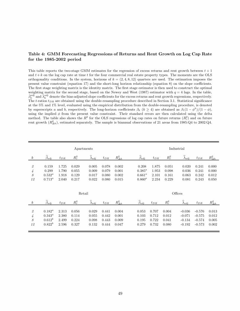
Table 4: GMM Forecasting Regressions of Returns and Rent Growth on Log Cap Rate

for the 1985-2002 period

This table reports the two-stage GMM estimates for the regression of excess returns and rent growth between t + 1and t+ k on the log cap rate at time t for the four commercial real estate property types. The moments are the OLSorthogonality conditions. In the system, horizons of k = (2, 4, 8, 12) quarters are used. The estimation imposes thepresent value constraint (equation 17) and the short-long horizon relationship (equation 8) on the slope coefficients.The first stage weighting matrix is the identity matrix. The first stage estimator is then used to construct the optimalweighting matrix for the second stage, based on the Newey and West (1987) estimator with q = 4 lags. In the table,β̂adj

k and λ̂adjk denote the bias-adjusted slope coefficients for the excess returns and rent growth regressions, respectively.

The t-ratios tDR are obtained using the double-resampling procedure described in Section 3.1. Statistical significanceat the 5% and 1% level, evaluated using the empirical distribution from the double-resampling procedure, is denotedby superscripts a and b, respectively. The long-horizon coefficients βk (k ≥ 4) are obtained as β1(1 − φk)/(1 − φ),using the implied φ from the present value constraint. Their standard errors are then calculated using the deltamethod. The table also shows the R2 for the OLS regressions of log cap rates on future returns (R2

r) and on futurerent growth (R2

∆h), estimated separately. The sample is biannual observations of 21 areas from 1985:Q4 to 2002:Q4.

Apartments Industrial

k bβadj tDR R2r

bλadj tDR R2∆h

bβadj tDR R2r

bλadj tDR R2∆h

2 0.159 1.725 0.029 0.005 0.078 0.002 0.208 1.875 0.051 0.020 0.241 0.0004 0.299 1.790 0.055 0.009 0.079 0.001 0.385a 1.953 0.098 0.036 0.241 0.0008 0.532a 1.918 0.129 0.017 0.080 0.002 0.661a 2.101 0.161 0.063 0.242 0.01212 0.713a 2.040 0.217 0.022 0.080 0.015 0.860a 2.234 0.229 0.081 0.243 0.050

Retail Offices

k bβadj tDR R2r

bλadj tDR R2∆h

bβadj tDR R2r

bλadj tDR R2∆h

2 0.182a 2.313 0.056 0.029 0.441 0.004 0.053 0.707 0.004 -0.036 -0.576 0.0134 0.343a 2.380 0.114 0.055 0.442 0.001 0.103 0.712 0.012 -0.071 -0.575 0.0128 0.612b 2.499 0.224 0.098 0.443 0.009 0.195 0.722 0.041 -0.134 -0.574 0.005

12 0.822b 2.596 0.327 0.132 0.444 0.047 0.279 0.732 0.080 -0.192 -0.573 0.002

49

Table 5: Structural Parameters for the 1985-2002 period

Panel A of this table shows the underlying structural parameters of the model described in equations (9)-(12) for thefour commercial real estate property types. The identification is obtained from the GMM estimates of Table 4 using themoment conditions as described in Appendix C. Panel B shows the implied annualized standard deviation of expectedreturns (std(Etrt+1)), expected rent growth (std(Et∆ht+1)), returns (std(rt+1)), and rent growth (std(∆ht+1)). PanelC shows the variance of expected returns as a fraction of total return variance (denoted by R2

Er) and the variance ofexpected rent growth as a fraction of total rent growth variance (R2

E∆h). Volatilities and covariances are expressedin annual terms. The sample is biannual observations of 21 areas from 1985:Q4 to 2002:Q4.

Panel A

Apartments Industrial Retail Offices

φ 0.883 0.848 0.885 0.949σξx × 102 1.946 1.701 1.377 1.414σξy × 102 0.838 0.727 0.469 0.400σξh × 102 4.306 4.928 3.478 5.153

τ 0.737 0.697 0.826 0.951ϑ × 104 1.294 1.006 -0.141 0.321

Panel B

Apartments Industrial Retail Offices

σξr × 102 8.498 7.414 4.606 7.260υ ≡ σ2

ξy/σ2ξx 0.186 0.183 0.116 0.080

std(rt+1) 0.095 0.081 0.055 0.085std(Etrt+1) 0.041 0.032 0.030 0.045std(∆ht+1) 0.056 0.056 0.044 0.068

std(Et∆ht+1) 0.035 0.026 0.026 0.045

Panel C

Apartments Industrial Retail Offices

R2Er 0.192 0.158 0.292 0.278

R2E∆h 0.403 0.221 0.366 0.429

50

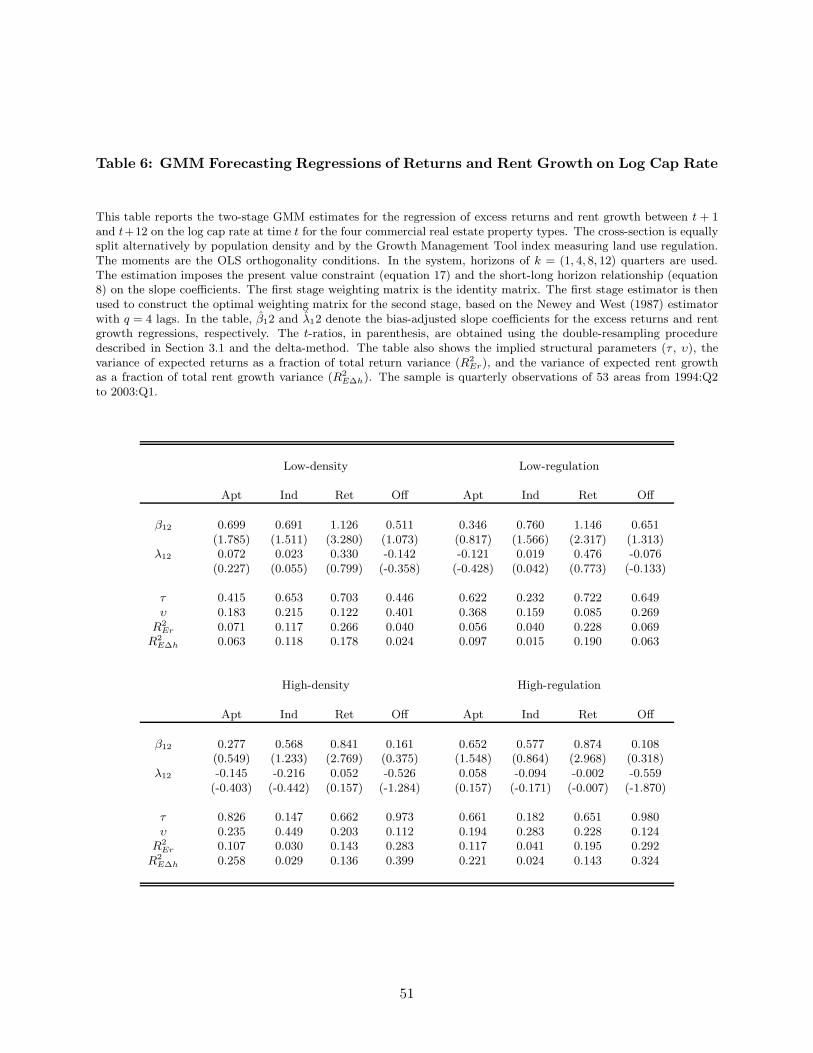
Table 6: GMM Forecasting Regressions of Returns and Rent Growth on Log Cap Rate

This table reports the two-stage GMM estimates for the regression of excess returns and rent growth between t + 1and t+12 on the log cap rate at time t for the four commercial real estate property types. The cross-section is equallysplit alternatively by population density and by the Growth Management Tool index measuring land use regulation.The moments are the OLS orthogonality conditions. In the system, horizons of k = (1, 4, 8, 12) quarters are used.The estimation imposes the present value constraint (equation 17) and the short-long horizon relationship (equation8) on the slope coefficients. The first stage weighting matrix is the identity matrix. The first stage estimator is thenused to construct the optimal weighting matrix for the second stage, based on the Newey and West (1987) estimatorwith q = 4 lags. In the table, β̂12 and λ̂12 denote the bias-adjusted slope coefficients for the excess returns and rentgrowth regressions, respectively. The t-ratios, in parenthesis, are obtained using the double-resampling proceduredescribed in Section 3.1 and the delta-method. The table also shows the implied structural parameters (τ , υ), thevariance of expected returns as a fraction of total return variance (R2

Er), and the variance of expected rent growthas a fraction of total rent growth variance (R2

E∆h). The sample is quarterly observations of 53 areas from 1994:Q2to 2003:Q1.

Low-density Low-regulation

Apt Ind Ret Off Apt Ind Ret Off

β12 0.699 0.691 1.126 0.511 0.346 0.760 1.146 0.651(1.785) (1.511) (3.280) (1.073) (0.817) (1.566) (2.317) (1.313)

λ12 0.072 0.023 0.330 -0.142 -0.121 0.019 0.476 -0.076(0.227) (0.055) (0.799) (-0.358) (-0.428) (0.042) (0.773) (-0.133)

τ 0.415 0.653 0.703 0.446 0.622 0.232 0.722 0.649υ 0.183 0.215 0.122 0.401 0.368 0.159 0.085 0.269

R2Er 0.071 0.117 0.266 0.040 0.056 0.040 0.228 0.069

R2E∆h 0.063 0.118 0.178 0.024 0.097 0.015 0.190 0.063

High-density High-regulation

Apt Ind Ret Off Apt Ind Ret Off

β12 0.277 0.568 0.841 0.161 0.652 0.577 0.874 0.108(0.549) (1.233) (2.769) (0.375) (1.548) (0.864) (2.968) (0.318)

λ12 -0.145 -0.216 0.052 -0.526 0.058 -0.094 -0.002 -0.559(-0.403) (-0.442) (0.157) (-1.284) (0.157) (-0.171) (-0.007) (-1.870)

τ 0.826 0.147 0.662 0.973 0.661 0.182 0.651 0.980υ 0.235 0.449 0.203 0.112 0.194 0.283 0.228 0.124

R2Er 0.107 0.030 0.143 0.283 0.117 0.041 0.195 0.292

R2E∆h 0.258 0.029 0.136 0.399 0.221 0.024 0.143 0.324

51

Table 7: GMM Forecasting Regressions of Returns and Rent Growth on Log Cap Rate

and Principal Components of Economic Variables

This table reports the two-stage GMM estimates for the regression of excess returns (r column) and rent growth (∆hcolumn) between t+1 and t+k for the four commercial real estate property types. Regressors are the log cap rate attime t, the three principal components extracted from eight economic variables at time t, and a coastal dummy. In thesystem, horizons of k = (4, 8, 12) quarters are used. The results refer to the 3-year (k = 12) horizon. The estimationimposes the present value constraint (equation 17) and the short-long horizon relationship (equation 8) on the slopecoefficients. The first stage weighting matrix is the identity matrix. The first stage estimator is then used to constructthe optimal weighting matrix for the second stage, based on the Newey and West (1987) estimator with q = 4 lags.In the table, cap denotes the bias-adjusted coefficient on the log cap rate. The t-statistics (in parenthesis below theestimates) are obtained using the double-resampling procedure described in Section 3.1. Statistical significance atthe 5% and 1% level, evaluated using the empirical distribution from the double-resampling procedure, is denoted bysuperscripts a and b, respectively. The table shows two specifications for each real estate property type: (1) includesthe cap rate, the three principal components and the coastal dummy, (2) includes just the principal components andthe coastal dummy. The table also shows the R2 for the corresponding OLS regressions for returns (R2

r) and rentgrowth (R2

∆h) at the k = 12 quarters horizon, estimated separately. The sample is annual observations of 53 areasfrom 1994 to 2001.

Apartments Industrialr ∆h r ∆h

cap 0.791b - 0.315 - 0.352b - -0.118 -(3.682) (1.913) (2.419) (-0.811)

pc1 -0.013a -0.018b -0.011 -0.012b -0.022b -0.009 -0.029b -0.007(-1.929) (-2.832) (-1.721) (-2.454) (-4.797) (-1.813) (-7.495) (-1.601)

pc2 -0.027b -0.015 -0.020a -0.016b -0.004 -0.011 -0.002 -0.008(-2.590) (-1.720) (-1.979) (-2.434) (-0.834) (-1.596) (-0.511) (-1.422)

pc3 -0.010 -0.001 -0.014a -0.006 -0.006 -0.003 -0.004 -0.004(-1.177) (-0.106) (-2.024) (-0.847) (-0.918) (-0.412) (-0.609) (-0.623)

coast 0.041b 0.028b 0.022b 0.013 0.020b 0.015a 0.016b 0.013a

(4.316) (2.897) (2.714) (1.722) (3.295) (2.182) (3.208) (2.236)

R2adj 0.302 0.138 0.138 0.090 0.219 0.057 0.077 0.042

Retail Officesr ∆h r ∆h

cap 0.914b - 0.118 - 0.246 - -0.370 -(5.236) (0.625) (1.309) (-1.830)

pc1 -0.017b 0.012b -0.025b 0.010b -0.026b -0.005 -0.034b -0.006(-4.581) (2.411) (-7.217) (2.457) (-3.786) (-0.602) (-5.701) (-0.810)

pc2 -0.011b -0.014a -0.013b -0.013a -0.005 -0.027b -0.003 -0.022a

(-2.337) (-2.055) (-3.014) (-2.238) (-0.625) (-2.336) (-0.422) (-2.246)pc3 -0.001 0.002 -0.003 0.002 -0.006 -0.016 -0.012 -0.011

(-0.188) (0.320) (-0.678) (0.343) (-0.513) (-1.186) (-1.122) (-0.991)coast -0.003 0.002 -0.004 0.004 0.033b 0.043b 0.026b 0.033b

(-0.550) (0.357) (-0.940) (0.986) (3.585) (3.259) (3.309) (2.513)

R2adj 0.368 0.063 0.136 0.073 0.169 0.123 0.101 0.096

52

Table 8: Portfolio Optimization

This table shows the optimal portfolio weights on stock and commercial real estate for the one-period quadraticutility maximization. For each asset, three specifications of weights are reported. The first specification correspondsto the unconditional problem, the second specification uses the dividend-price ratio as conditioning variable, thethird specification conditions on both the dividend-price ratio and the cap rate. The corresponding average excessreturn of the optimal portfolio (E(Rp)), its standard deviation (σp), and its Sharpe ratio (SRp) are also displayed.The annualized equalization fee is defined as fee that the investor would be willing to pay to have access to theconditional information. Bootstrapped t-statistics are shown in parenthesis below the estimates. The sample isbiannual observations from 1986:Q2 to 2002:Q4.

Unconditional case Conditional on dp Conditional on dp and cap

Stock Constant 0.582 0.530 0.664(2.889) (2.912) (2.711)

dp 0.528 0.732(2.060) (2.388)

cap 0.881(2.182)

Cre Constant 0.167 0.291 0.180(0.223) (0.388) (0.233)

dp -1.627 -1.141(-2.650) (-2.163)

cap 0.297(2.198)

E(Rp) 0.037 0.084 0.132σp 0.083 0.117 0.135

SRp 0.446 0.716 0.976Equalization fee 0.030 0.066

53

Figure 1: Cap rates and dividend-price ratio

This figure plots the cap rate for the commercial real estate (evaluated as average of the population-weighted averagesof each property type) and the dividend-price ratio for the CRSP value-weighted portfolio, for the 1994:Q2 - 2003:Q1quarterly series (top panel) and for the 1985:Q4 - 2002:Q4 semi-annual series (bottom panel). The dividend-priceratio series is break-adjusted in 1992.

1995 1996 1997 1998 1999 2000 2001 2002 20030.085

0.09

0.095

0.1

Cap R

ate

Year

1995 1996 1997 1998 1999 2000 2001 2002 20030.01

0.016

0.022

0.028

D/P

Commercial RE

CRSP

1986 1988 1990 1992 1994 1996 1998 2000 20020.08

0.0867

0.0933

0.1

Cap R

ate

1986 1988 1990 1992 1994 1996 1998 2000 20020.02

0.04

0.06

0.08

D/P

Year

Commercial RE

CRSP

54

Figure 2: Cross-sectional dispersion in cap rates

This figure reports the 5th and 95th percentile (dotted line), and the mean (solid line) of the cross-sectional distributionof cap rates for the four property types. The sample is quarterly observations of 53 metropolitan areas from 1994:Q2to 2003:Q1.

1996 1998 2000 2002

0.07

0.08

0.09

0.1

0.11

Apartments

Cap R

ate

Year1996 1998 2000 2002

0.07

0.08

0.09

0.1

0.11

Industrial

Cap R

ate

Year

1996 1998 2000 2002

0.07

0.08

0.09

0.1

0.11

Retail

Cap

Rate

Year1996 1998 2000 2002

0.07

0.08

0.09

0.1

0.11

Offices

Cap

Rate

Year

55

Figure 3: Beta and Lambda as a function of τ and υ

This figure plots the slope predictive coefficients of the return regression β and rent growth regression λ, as functionof the structural parameters τ (top two plots) and υ (bottom two plots) using equations (15) and (16). In theexpressions, we set φ = 0.95 and ρ = 0.98.

−1 −0.5 0 0.5 10.02

0.04

0.06

0.08

0.1

τ

β

υ=0.13

υ=0.19

υ=0.25

τ

λ

−1 −0.5 0 0.5 1−0.06

−0.04

−0.02

0

0.02

0.04

υ=0.13

υ=0.19

υ=0.25

0 0.2 0.4 0.6 0.80

0.2

0.4

0.6

0.8

υ

β

τ=0.30

τ=0.70

τ=0.90

υ

λ

0 0.2 0.4 0.6 0.8−0.1

0

0.1

0.2

0.3

0.4

0.5

0.6 τ=0.30

τ=0.70

τ=0.90

56

Figure 4: Portfolio weights on aggregate stock market and commercial real estate

This figure plots the time series of conditional portfolio weights on the stock (top panel) and on the aggregatecommercial real estate (bottom panel). The dotted line displays the corresponding unconditional weights. Thesample is biannual observations from 1986:Q2 to 2002:Q4.

1986 1988 1990 1992 1994 1996 1998 2000 2002 2004

0

1

2

3

1986 1988 1990 1992 1994 1996 1998 2000 2002 2004

−1

0

1

2

57