stochasticpricedynamicsimpliedbythelimit orderbook · its distance to the current best offer, or...
TRANSCRIPT
arX
iv:1
105.
4789
v1 [
q-fi
n.T
R]
24
May
201
1
Stochastic Price Dynamics Implied By the Limit
Order Book
Alex Langnau
Allianz Investment Management
Yanko Punchev
LMU Munich
Abstract
In this paper we present a novel approach to the determination of fat tails infinancial data by studying the information contained in the limit order book. In anorder-driven market buyers and sellers may submit limit orders, which are executedif the price touches a pre-specified lower, respectively higher, limit-price. We showthat, in equilibrium, the collection of all such orders - the limit order book - impliesa volatility smile, similar to observations from option pricing in the Black-Scholesmodel. We also show how a jump-diffusion process can be explicitly inferred toaccount for the volatility smile.
1 Introduction
The organization of a marketplace where buyers and sellers meet to exchange a welldefined asset naturally lies at the heart of the price discovery process. Traditionallythis is done by specialist market makers with a mandate to match bid and ask quotesfrom market participants. Such market-order driven ways of trading define the most“impatient” form of interactions in the market place - orders are executed immediatelyas soon as a counterparty is identified that matches the order even at the expense ofgetting “filled” at a price that is suboptimal to the initiator of the trade. Such slippage issymptomatic of market-orders and can be viewed as the “price to pay” for the impatienceto execute. The latter can be avoided by trading limit-orders instead of market-orders.Each limit order includes a price level and a quantity. A seller would specify a pre-definedexecution price level that is typically set above the current market price, whereas a buyerwould like to purchase below the current market price at a limit-price of her choice. Theimportant difference to market-orders is that limit-orders never get filled suboptimally,but may rather not get filled at all or filled only partially in some cases. Hence the marketparticipant needs to exercise “patience” to see an order completed and to be rewardedwith a premium to current levels. The higher the limit-order price level, the higher thepotential rewards and the higher the patience required to see a trade completed in time.
All limit orders are typically collected by the exchange in a limit order book (LOB)that can be accessed by all market participants. According to P. Jain [Jai03], currentlymore than half of the world’s markets are order-driven.
This raises a sequence of interesting theoretical questions about LOBs such as how oneshould optimally position oneself for trading in a LOB? What is the information containedin a LOB and when is it in equilibrium? The recent public availability of LOB data hassparked extensive studies on the structure of LOBs. The work of J. Bouchaud et al.
1

[BMP02] provides useful insights into the shape of the LOB from a statistical standpoint.The study conducted by A. Ranaldo [Ran04] sheds light on aspects of the behavior ofmarket participants as represented by the change of their impatience preferences as afunction of the bid-ask spread. Further, Z. Eisler et. al in [EKL07] give a detailed lookat how the LOB behaves on different time scales. In [CST08] a stochastic model forthe dynamics of the LOB in continuous time has been developed, allowing for simplecalibration and explicit calculation of certain probabilities of interest. M. Bartolozzi[Bar10] proposes a multi-agent model for the dynamics of the LOB, with a particularfocus on capturing key features of high-frequency trading. M. Avellaneda et al. [AS06]also propose a probabilistic framework for a utility optimizing agent in the context ofhigh-frequency markets. A study conducted in Spanish equity markets by R. Pascualet. al [PV08] focuses on what pieces of information of the LOB is significant and findsthat the information is concentrating around the best bid and ask orders, while ordersfurther out in the LOB do not significantly contribute to the price formation process.Somewhat similarly, I. Rosu [Ros10] proposes a dynamic model for order-driven marketswith asymmetric information. He argues that the price impact of market orders is moresignificant than the impact of limit orders by an order of magnitude. Furthermore, R.Cont et. al [CKS10] study the price impact of order book events and find a surprisinglysimple linear dependence between price changes and an indicator they introduce, whichmeasures the imbalances between the order flow on the buy and sell sides of the LOB. In[TKF09] a study of the dynamics of different indicators, such as the bid-ask imbalance,is conducted before and after large LOB events and finds significant dependencies.
The objective of this paper is to study consequences in situations when a LOB is inequilibrium. Following arguments by Rosu [Ros08], equilibrium occurs when, at any time,there exists an impatience rate, independent of (limit-order price) level, which “discounts”limit-sell orders at higher prices in favor of smaller once. Thus an impatience rate strikesa consistent compromise between higher prices on the one hand, and longer expectedpassage-times to fill on the other hand, throughout the LOB. We study the LOB dataof the DAX future and show that the assumption of a geometric Brownian motion forthe price dynamics implies a volatility smile which is reminiscent of the volatility smileobserved in option markets. This allows us to conjecture and re-engineer non-trivialdynamics underlying the LOB. We show that the assumption of a double-exponentialjump dynamics provides a satisfactory description of the data. Hence this work providesfurther new evidence for the occurrence of fat tails in financial data. In addition it providesa novel approach for the determination of jump parameters in finance.
The paper is outlined as follows - first we formalise the general notion of an impatiencerate - the quantifier of the trade-off between waiting longer but executing the order at abetter price. We then test the assertion, that the impatience rate is level-independent, byassuming that the prices follow a geometric Brownian motion (GBM). We find that theGBM cannot account for a consistent impatience rate, and observe a volatility smile - ifthe impatience rate were to be level-independent then limit-orders at higher levels implyan ever increasing volatility. Considering the evidence we augment the price process byadding jumps. We conclude by providing evidence, that the double-exponential jump-diffusion (DEJD) price process admits an impatience rate independent of the limit-orderlevel.
2

2 Impatience Rate
In this work we aim to extract empirically testable pieces of information from the LOB,which are also pertinent to order-driven markets, and are as much as possible independentof the model at hand. In reviewing the literature on LOB modelling, a distinction betweenpatient and impatient agents has turned out to be the common denominator of a muchof the research. Specifically in his seminal paper on LOB dynamics, Rosu [Ros08] reliesexplicitly on a parameter r, the impatience rate, which acts as a discounting or penalizingfactor for waiting longer for a better fill price. Rosu further proposes an equilibriummodel, in which agents maximize their utility according to the following utility function:
ft := Et[Pτ − r(τ − t)], and − gt := Et[−Pτ − r(τ − t)] (1)
where ft is the expected seller utility at time t, τ is the time of the limit order execution, Pτ
is the limit order price and r is the common impatience rate of sellers and buyers. Similarly−gt is the buyer’s utility. Regardless of specific price dynamics assumptions and LOBmodel, a limit order far away from the current price will take longer to fill, so r weighsthe benefit of a better fill price, which increases utility, by penalizing for waiting longerand decreasing utility. So the impatience rate should quantify this fundamental trade-offbetween waiting longer to execute at a better price and waiting less, but executing at aworse price. Consequently, if the LOB is in a state of equilibrium, and if capital marketsare efficient, the impatience rate should be the same across limit-order levels.
I. Rosu in [Ros08] shows that such an equilibrium exists in his theoretical framework,and empirical testing should provide evidence whether the LOB is efficient, or at leastimply what the price process should look like, if the assumption of information efficiencywere to hold. Despite playing such a central role in many works on limit-order markets,the properties of the impatience rate r have not been examined.
The utility function as given in (1) is somewhat unfortunate. On the on hand, itdepends on the absolute level of the limit order price, Pτ , which leads to different resultseven in Rosu’s model for markets, which are equivalent up to a price scaling constant.Also, this approach suppresses an important characterization of the limit order, namelyits distance to the current best offer, or at least to the mid price. In (1) this is expressedonly indirectly through the expected hitting time E[τ ]. At this point another drawbackof this particular utility becomes apparent - the fact that E[τ ] = ∞, if the asset price ismodelled by an exponential Brownian motion without drift, or if the drift is in a directionaway from the submitted limit order.1
Since (1) depends on the absolute level of the price, and would generally be infinity fora Brownian motion price process we investigate a different utility function. We considerthe currency value of the distance-to-fill, i.e. how much the best offer has to travel untilit meets a trader’s limit order, discounted by the impatience rate in a quite literal sense:
UD(r) = |D|E[exp(−rτS+D)|S0 = S] (2)
D ∈ R is the distance from the limit order to the best offer S0 at time t = 0. FurtherτS+D is the first hitting time of the price process St describing the evolution of the bestoffer, started in S0:
τS+D := inft≥0
St = S +D.
1For a discussion of how the GBM should be specified, so that the expected hitting time is finite cf.M. Yor et. al [JYC09].
3

3 A Pure Diffusion Setting
We first adopt a model in which the asset price (St)t≥0 is a geometric Brownian motion(GBM). Specifically let
(Ω,F , (Ft)t≥0 ,P
)be a filtered space 2, and (St)t≥0 be a stochastic
process on this filtered space, whose dynamics are given by the stochastic differentialequation (SDE)
dSt = Stµdt + StσdBt , S0 = S
where S, σ > 0, µ ∈ R and (Bt)t≥0 is a standard Brownian motion, started in 0. The SDEhas the exact solution 3:
St = S exp
((µ−
σ2
2
)t+ σBt
)(3)
We define the asset price log-returns over an interval ∆t > 0 by
l(∆t) := ln
(St+∆t
St
),
and establish the following results:
E[l(∆t)] = E
[(µ−
σ2
2
)∆t + σB∆t
]=
(µ−
σ2
2
)∆t (4)
V[l(∆t)] = E
[((µ−
σ2
2
)∆t + σB∆t
)2]−
((µ−
σ2
2
)∆t
)2
= σ2∆t (5)
Further we note that the Laplace transform of the first hitting time at level z ∈ R
τz := inft≥0
Bt = z
of a standard Brownian motion with drift µ
B(µ)t := µt+Bt
is given by4
E[exp(−rτz)] = exp(µz − |z|
√2r + µ2
)(6)
for some r > 0. Finally a simple transform is needed to obtain a closed formula for theexpected utility:
τS+D = inft≥0
St ≥ S +D = inft≥0
St = S +D
= inft≥0
S exp
((µ−
σ2
2
)t+ σBt
)= S +D
= inft≥0
µ− σ2
2
σ︸ ︷︷ ︸=:µ
t+Bt =ln(S+DS
)
σ︸ ︷︷ ︸=:z
(7)
= τz, S ∈ R+ D ∈]− S,∞[
2In the rest of this paper we will always assume, that any stochastic process we introduce is adaptedto this generic filtered space and its dynamics are given with respect to the physical probability measureP.
3Cf. [Shr04]4Cf. [BS96] (page 223, 2.0.1).
4

Now τz is the first hitting time of a standard Brownian motion with drift µ for the hittinglevel z ∈ R. Notice that we allow z < 0, so that we can use the same result for hittinglevels above the current price, as well as below the current price. In particular we can usethe same formula for the bid and for the ask side of the book. Now we are in a positionto compute explicitly for D ∈ R \ 0, r, S > 0:
UD(r) = |D|E[exp(−rτS+D)|S0 = S]
= |D|E[exp(−rτz)]
= |D| exp(µz − |z|
√2r + µ2
)
= |D| exp
(µ− σ2
2
)ln(S+DS
)
σ2−
∣∣ln(S+DS
)∣∣σ
√√√√2r +
(µ− σ2
2
2
)2 (8)
In order to calibrate our model to market data, we need to estimate the drift and thevolatility of the GBM. We do this by estimating the sample mean and standard deviationof the log-returns market mid-prices at equidistant time points, with a constant timeinterval of ∆t. Recall that Mt, the mid price at time t, is simply the mid-point of the askprice at level zero A
(0)t and the bid price at level zero B
(0)t :
Mt :=B
(0)t + A
(0)t
2, B
(0)t , A
(0)t > 0
We do a rolling estimate for each data point i in equidistantly spaced LOB (i.e. ti −ti−1 = ∆t) using a standard point estimate of the sample mean, based on the last thirtyobservations prior to the current point:
mi(∆t) :=1
30
30∑
k=1
log
(Mi−k
Mi−k−1
)
Similarly we estimate the standard deviation of the log-returns by:
si(∆t) :=
√√√√ 1
29
30∑
k=1
(log
(Mi−k
Mi−k−1
)−mi(∆t)
)2
(9)
Notice that k starts at one, ensuring that our current estimate of the sample mean andstandard deviation uses only past data. Recalling the expressions for the expected value(4) and the variance (5) of a GBM, we first substitute si(∆t)2 for V[l(∆t)] in (5) to obtainthe simple rolling estimate:
σ2∆t = si(∆t)2 (10)
Plugging this expression in (4), and substituting mi(∆t) for E[l(∆t)], we estimate:
mi(∆t) =
(µ−
si(∆t)2
2
)∆t
⇒µ∆t = mi(∆t) +si(∆t)2
2(11)
Now our model is thoroughly specified and we are in a position to calculate the expectedutility at any point in time, given the value of the impatience rate at that point. Since,
5

however, the impatience rate is precisely what we would like to estimate, we need anadditional assumption about the whole setting. Considering that the LOB is in an equi-librium when the expected utility of all participants on each side of the book is the same,so no one has an incentive to put in their order at a different level5, we assume that theexpected utility is constant over short periods of time, and that it evolves fairly smoothlyin time, as the expectations of the market participant on each side of the book for thefuture direction of price movements changes through time. By starting at some reasonablevalue for the expected utility we can fit the impatience rate stepping through time, withthe objective of keeping the utility stepwise constant achieving a smooth fit.
A clearer specification of the algorithm impatience rate estimation by fitting the ex-pected utility to market data in a GBM framework is due. The inputs required are thefollowing:
• N - the number of data points in the reconstructed LOB with equidistant spacingof ∆t. The results presented in this paper are for ∆t = 30 seconds.
• “steps” - indicates the number of data points, over which the expected utility is tobe held constant, in order to minimize an error function. In this paper we presentresults for “steps”=2, in order to compare the results better to the DEJD model;
• m - a vector of size N , containing the rolling estimates for the mean of the observedlog-returns where the time interval between observations is ∆t. Note that mj , theestimate at time tj , is based on the log-returns at thirty observations prior to tj, sono peeking in the future is allowed;
• s - a vector of size N , containing the rolling estimates for the standard deviation ofthe observed log-returns where the time interval between observations is ∆t, whereagain estimates are based on a past data only;
• U0 - an initial estimate for the expected utility;
• r0 - an initial estimate for the impatience rate;
The outputs are two vectors U and r, each of size N , containing the expected utility andthe impatience rate through time.
The particular choice of the error function in row 9 is a natural one - it collectsthe differences in utilities step by step, scaling each error by the mean of both adjacentutilities, ensuring the minimization algorithm would not just choose a large r to convergeby essentially driving all utility down to zero. Particular care has to be taken whenchoosing ǫ, δ and other minimization algorithm break criteria in order to ensure timelyconvergence. Also one has to consider what ∆t to choose in order to reduce the numberof time steps of the immense data set the LOB offers per day (in our case about 450,000observations per day in the LOB organization of Figure 16 in Appendix C). Furtherwhen choosing “steps”, one faces the trade-off between smoothness of U for an increasingnumber of “steps” on the one hand, against potential convergence problems, as well as amore noisy r.
5Cf. [Ros08]
6

Algorithm 1 Estimation of the impatience rate in a GBM settingInputs: N, steps, m, s, U0, r0
1: r = r02: for i=1:steps:N do
3: while error(r) > ǫ & Tolerance > δ do
4: ri := minr>.01error(r)5: WHERE error(r) is6: for j=i:steps+1 do
7: calculate Uj according to (8) using mj , sj, r8: end for
9: error(r) =∑steps+1
j=i
(Uj − Uj−1
0.5(Uj + Uj−1)
)2
10: end while
11: end for
Outputs: U , r
4 Results For a Pure Diffusion
We find, that in a GBM setting, the impatience rate r is not constant across levels,meaning that either the market is not in equilibrium, as contended in [Ros08] and dictatedby the efficient markets hypothesis, or that the GBM framework is an inadequate cannotdescribe the LOB equilibrium. We further observe a volatility smile (see Figure 5), whichleads us to assume a jump-diffusion process for the asset price dynamics.
All results presented here are based on the following parameters: ∆t = 30 sec; “steps”= 2; r0 = 1 and U0 is calculated according to (8) for r = r0 = 1. It should be noted,that we achieved very similar results for “steps=15” and for “steps=30”, indicating thefitting algorithm is independent of the particular time-stepping procedure. The resultsare also the same for different starting r0 and U0, providing evidence that the problem iswell-defined and fitting procedure is also well-posed.
Our results are based on nearly three months of LOB data of the DAX future fromJune to August 2010. Analysis of the data revealed properties of the impatience rate andthe expected utility which have been very consistent throughout trading days. We willillustrate them based on a representative day of our data set - 20 August, 2010 - and referthe reader to the appendix for descriptive statistics for each day.
In Figure 1 we present the impatience rate r as a function of the risk-adjusted relativedistance-to-fill
z =
log
(S +D
S
)
σ, (12)
for the sell side of the LOB. If r were to be constant, strains of flat lines, each strainindicating a different market mode, should be observable. Instead, for different levels ofexpected utility, the impatience rate assumes a power law of the form
r =1
zα(13)
for some α > 0.The relationship demonstrated in Figure 1 provides evidence, that the impatience
rate is primarily a function of the estimated volatility and the distance-to-fill D. A first
7

0 1 2 3 4 50
2
4
6
8
10
12
14
r =
Impa
tienc
e R
ate
z = Risk−Adjusted Relative Distance−To−Fill
Figure 1: Impatience rate (r, y-axis) against risk-adjusted relative distance-to-fill (z, x-axis) for the sell side of the book. The fitting procedure reveals a power law for r, whichis driven by both - the estimated volatility s and the absolute distance-to-fill D. (FDAX,August 20, 2010)
conclusion is that in the GBM model the impatience rate is not constant across differentlevels. In particular it cannot extract solely the information content about the trade-offbetween a better fill price and a longer expected waiting time, but much rather it stillcontains information about the volatility and the distance-to-fill. Next, in Figure 2 weshow a log-log plot which suppresses the power law relationship between r and z andreveals the different strains of this relationship for different levels of expected utility. Therelative level of expected can be interpreted as indicative of prevailing market sentimentand therefore different levels of expected utility represent different market modes, andsharp changes in the absolute value of utility point to a sentiment shift.
In figure 3 we present the expected utility compared to the mid-price through time.Changes in the direction of the expected utility, indicate numerical instability and can beinterpreted as an indication, that a shift in sentiment of the respective market participants(here - the sellers), is taking place. A more detailed analysis showed that while indeedprice direction and expected utility changes are concurrent, the latter is not a reliablepredictor of the former.
In Figure 4 a comparison of the impatience rate and the mid-price is given. Oneof the objectives of this research is to conclude whether the impatience rate is somehowindicative of future price movement, or if it contains any other piece of useful information.The intuition is that on, per example, the sell side of the book, an increasing impatiencerate r indicates, that sellers are becoming eager to get out of their holdings, so a pricedeterioration can be anticipated.
While testing has revealed, that sharp changes in the mid-price are accompanied a
8

10−1
100
101
10−1
100
101
r =
Impa
tienc
e R
ate
z = Risk−Adjusted Relative Distance−To−Fill
Figure 2: log10 of the impatience rate (r, y-axis) against log10 of the risk-adjusted relativedistance-to-fill (z, x-axis) for the sell side of the book. Notice the different linear (expo-nential on a linear scale) strains, which indicate the same power relationship between rand z for different levels of the expected utility. (FDAX, August 20, 2010)
shift in the opposite direction of the sell-side impatience rate, the direction of r is not areliable indicator of future price movements, since there are false outbreaks. Also pricechanges, which have not occurred abruptly enough, may not be captured by a significantchange in r and thus missed. Notice also how the impatience tends to fluctuate, arounda stable state, when the price is trending sideways. This is a particular consequence ofthe fact that the impatience rate is a function of the distance-to-fill - the fluctuationsindicate that the impatience rate needs to assume a different value for new values ofD, in order to keep the expected seller utility smooth. As a result regression analysishas showed no significant relationship between the estimated impatience rate and futuremid-price returns. The results for the buy-side of the LOB are similar and a side-by-sidecomparison of sell and buy side results can be seen in the appendix.
5 Volatility Smile
The results reveal that the impatience rate is not constant across LOB levels and in thismodel framework cannot be used as a consistent quantifier of the trade-off between abetter fill price a longer expected time-to-execution. Further analysis suggested that theimpatience rate in a GBM model is a function of the distance-to-fill and of the estimatedvolatility. Intuitively the market participants, who place their orders further out in theLOB, imply a much higher volatility than the observed. It seems as if traders who placeorders at higher levels in the LOB are betting on a sharp price change in the desireddirection. In order to analyse this further, we take a look at the LOB implied volatility,
9

2 3 4 5 6 7 8
x 104
0.24
0.26
0.28
0.3
0.32
0.34
0.36
Exp
ecte
d U
tility
Time2 3 4 5 6 7 8
x 104
5980
6000
6020
6040
6060
6080
6100
Mid
Pric
e
Figure 3: The expected seller utility U (left axis) and the mid-price (right axis) throughtime (x-axis) on a single trading day. Notice the initial drop from the initial estimate toa level which is reflecting the actual expected utility given the impatience rate r, and thesubsequent smoothness of the evolution of the utility. Jumps indicate a change in theutility level and correspond to a different linear strain in the relationship between r andz, as demonstrated in the previous figure. (FDAX, August 20, 2010)
which we define to be the volatility σ for which
UD(r) = UD(r, σ) = c (14)
for some positive constant c. As we have already established, the impatience rate dependson D, and on σ, so we would like to separate and measure the two effects. To this endwe choose an arbitrary, but reasonable, constant c for the utility level and also fix theimpatience r at some constant level. Both are held constant throughout a whole tradingday, and we fit for σ, to derive the implied volatility which keeps the impatience rateconstant at r and the expected utility level UD(r, σ) constant at a level c for the entiretrading day. What we discover is a volatility smile, being implied by the LOB, as isdemonstrated in Figure 5. Essential this shows, that the GBM underweights limit ordersat higher levels - the process’ volatility is insufficient for it to reach these limits in duetime, so the volatility has to be tuned up to account for the dynamic equilibrium, and formarket efficiency to hold.
The empirical work conclusively shows, that in a GBM setting, there is no unifyingimpatience rate across the different levels in the LOB. It has turned out that it is a functionof both - the volatility term σ of the stochastic process, and of |D| - the distance-to-fill. Itis inversely related to the volatility, i.e. the higher the volatility, the lower the impatiencerate, on either side of the book. It means that it becomes “easier” for the process toreach an order, which is at a higher level in the book, which is in turn necessary due the
10

2 3 4 5 6 7 8
x 104
0
5
10
15
Impa
tienc
e R
ate
Time2 3 4 5 6 7 8
x 104
5950
6000
6050
6100
Mid
Pric
e
Figure 4: The seller impatience rate r (left axis) and the mid-price (right axis) throughtime (x-axis) on a single trading day. Intuitively a rise in the seller impatience rate shouldprecede or accompany a fall in the price. (FDAX, August 20, 2010)
assumption that the expected utility is the same at all levels of the book, and evolvessmoothly through time.
In the same way, the impatience rate is a function of the distance-to-fill. It plays therole of a “volatility-compensator”, keeping the expected utility U constant across levelsfor different values of |D| . The impatience rate needs to be very small for large |D| inorder to compensate for the decrease in utility, as τ becomes too big. Since the volatilityis fixed by empirical observations, and E[τ ] is known6 to grow exponentially with risingdistance, it is a direct consequence of the GBM framework, that r follows an exponentialdecay law for an increasing |D| and a falling σ.
The inverse power-law between the impatience rate and the observed volatility isespecially clearly observable in the volatility smile. This surprising discovery highlights thefact that in order to achieve utility equilibrium one has to tune up the process’ volatility,so that limit orders placed further away from the mid-price have a higher chance ofexecution. Intuitively one may argue, that market participants place limit orders furtherout in the LOB, because they anticipate a large block of orders being placed at once, sothat lower level limit orders get immediately filled, leaving the agent’s order as the bestor even filling it.
A critical argument for jump augmentation is based on the observed “volatility smile”,a phenomenon well known from option pricing.7 There are already many models in optionstheory which account for the smile. Regarding the principle idea of the solution, thereare two broad classes of approaches to incorporate this phenomenon in the price process.
6Cf. [BS96].7Cf. [Der03], [SP99] on more about the volatility smile in the context of option pricing.
11

0.9992 0.9994 0.9996 0.9998 1 1.0002 1.0004 1.0006 1.00081
1.2
1.4
1.6
1.8
2
2.2
2.4x 10
−4
(S+D)/S
Sig
ma
Figure 5: The volatility smile, as implied by the LOB. A scatter plot of the impliedvolatility σ (y-axis) and the relative distance-to-fill (S+D)/S (x-axis) form what resemblesa volatility smile as known from equity options pricing. The plot reveals a whole day’sworth of data. σ values to the left of one are derived from the bid-side of the LOB, andto the right - from the ask-side. This instance of the smile was derived for U = 0.2355and r = 0.5 (FDAX, August 20, 2010)
One is to assume a stochastic process for the volatility term in front of the Brownianmotion. The other is to add a jump process to the Brownian motion. While it might seemsomewhat natural that the volatility itself should also be a process rather than a constantterm, the dynamics that are usually used to model the evolution of the volatility throughtime are not necessarily intuitive.8 On the other hand, the idea, that price processes havejumps is considered characteristic of financial time series9 and is readily observable10. Incombination with the intuition, that limit order traders position themselves at the outerlevels in anticipation of a block-trade, or a sharp price movement, we are lead to extendthe GBM to a jump-diffusion by incorporating a jump process, i.e. a process of the form:
dSt = µStdt+ σStdBt + StdJt, Jt =Nt∑
i=i
Yi
where Jt is a time-homogeneous compound Poisson process, whose jump sizes (Yi)i∈N area family of independently and identically distributed (iid) random variables.11
8Cf. [Bro09]9Cf. [Bro09], [BD02], [BD89],[MFE05]
10Cf. [Bro09],[MLMK08], [AM10]11Cf. [Gat10]
12
6 A Jump-Diffusion Setting
Lead by the observation of a volatility smile and the intuition that far-off limit orders areunderweighted, in the sense that in the geometric Brownian motion (GBM) frameworkhigh-level orders are too difficult to hit, we extend our asset price model to include jumps.In this way we will be able to account for the observed empirical phenomena and serveintuition. Due to the increased flexibility of the models we are also certain to obtain abetter fit of a period-wise constant impatience rate to the market data.
Since the success of the Black-Scholes-Merton formula for equity option valuation,which underlies a geometric Brownian motion, a number of jump-diffusion models havebeen proposed as an extension to the original model. We are going to use the DoubleExponential Jump Diffusion (DEJD) model, as proposed by Kou in [Kou02] and exten-sively studied by Kou and Wang in [KW03]. Our choice is lead by our specific interestof the Laplace transform of the first passage time of the asset price. As is demonstratedin [KW03], the model offers a closed-form solution (up to finding the zeros of a rationalfunction) for the Laplace transform.
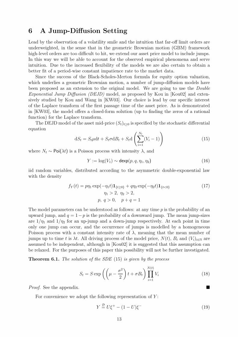
The DEJD model of the asset mid-price (St)t≥0 is specified by the stochastic differentialequation
dSt = Stµdt + StσdBt + Std
(Nt∑
i=1
(Vi − 1)
)(15)
where Nt ∼ Poi(λt) is a Poisson process with intensity λ, and
Y := log(V1) ∼ dexp(p, q, η1, η2) (16)
iid random variables, distributed according to the asymmetric double-exponential lawwith the density
fY (t) = pη1 exp(−η1t)1t≥0 + qη2 exp(−η2t)1t<0 (17)
η1 > 2, η2 > 2,
p, q > 0, p+ q = 1
The model parameters can be understood as follows: at any time p is the probability of anupward jump, and q = 1−p is the probability of a downward jump. The mean jump-sizesare 1/η1 and 1/η2 for an up-jump and a down-jump respectively. At each point in timeonly one jump can occur, and the occurrence of jumps is modelled by a homogeneousPoisson process with a constant intensity rate of λ, meaning that the mean number ofjumps up to time t is λt. All driving process of the model price, N(t), Bt and (Vi)i∈N areassumed to be independent, although in [Kou02] it is suggested that this assumption canbe relaxed. For the purposes of this paper this possibility will not be further investigated.
Theorem 6.1. The solution of the SDE (15) is given by the process
St = S exp
((µ−
σ2
2
)t+ σBt
)N(t)∏
i=1
Vi (18)
Proof. See the appendix.
For convenience we adopt the following representation of Y :
YD= Uξ+ − (1− U)ξ− (19)
13

where U ∼ Ber(p) is a Bernoulli random variable, indicating that an up-jump occurs withprobability p, ξ+ and ξ− are both exponential random variables with means 1/η1 and 1/η2respectively, corresponding to the mean up-jump and mean down-jump sizes. All threerandom variables are assumed to be independent.
Theorem 6.2. The asset mid-price model specified by (18) and (19) where Y = log(V1)has the following properties
a) EY = pη1
− qη2
and VY = pq(
1η1
+ 1η2
)2+(
pη21
+ qη22
);
b) E[V ] = q η2η2+1
+ p η1η1−1
, and
V[V ] = pη1
η1 − 2+ q
η2η2 + 2
−
(p
η1η1 − 1
+ qη2
η2 + 1
)2
, η1, η2 > 2;
c) The first two moments of the “Poisson product” Pt :=∏Nt
i=1 Vi are:
• E[Pt] = exp(tλ(E[V ]− 1)) and
• E[P 2t ] = exp(tλ(E[V 2]− 1));
d) ESt = S exp(µt)E[Pt] and VSt = S2e2µt(eσ
2tE[P 2
t ]− E[Pt]2)
e) For l(∆t), the log-returns over a period ∆t, we have:
• E[l(∆t)] =(µ− σ2
2
)∆t+ λ
(pη1
− qη2
)∆t and
• V[l(∆t)] = σ2∆t + λ∆t(
2pη21
+ 2qη22
).
Proof. See the appendix.
Observing that V[V ] = ∞ for η1 ≤ 2, as shown in the proof of b), we are lead toimpose this constraint when modelling the asset price. Since there is no intuitive reasonto prefer a priori any price direction we make the same assumption for η2 in (17). Itessentially means, that mean jump sizes cannot exceed 50%.
6.1 First Passage Time Results
Here we present the results of Kou/Wang for the first passages times of a double expo-nential jump diffusion process, as given in [KW03]. Consider the DEJD proces
Xt = σBt + µt+
Nt∑
i=1
Yi; X0 := 0 (20)
where (Bt)t≥0 is a standard Brownian motion, (Nt)t≥0 is a Poisson process with intensityrate λ, µ and σ > 0 are respectively the constant drift and the volatility of the diffusionpart of the process. The family of the jump-sizes (Yi)i∈N is independent and identicallydistributed according to a a double-exponential distribution with density fY as given in(17). We are interested in the Laplace transform of τb, the random variable specified bythe first passage time of a boundary b:
τb := inft≥0
Xt ≥ b, b > 0 (21)
14

The infinitesimal generator of the jump diffusion process (20) is given by
Lu(x) =1
2σ2u′′(x) + µu′(x) + λ
∫ ∞
−∞
(u(x+ y)− u(x)
)fY (y)dy (22)
for all twice continuously differentiable functions u(x). Further, suppose θ ∈] − η2, η1[.The moment generating function of the jump size Y is given by:
E[exp(θY )] =pη1
η1 − θ+
qη2η2 + θ
, (23)
from which the moment generating function of Xt can be obtained as
ϕ(θ, t) := E[exp(θXt)] = exp(G(θ)t),
where the function G(·) is defined as
G(x) := xµ+1
2x2σ2 + λ
(pη1
η1 − x+
qη2η2 + x
− 1
)(24)
Lemma 6.1. The equationG(x) = α for all α > 0 (25)
has exactly four roots: β1,α, β2,α, −β3,α, −β4,α where
0 < β1,α < η1 < β2,α < ∞, 0 < β3,α < η2 < β4,α < ∞
Proof. Cf. [KW03] (page 507, Lemma 2.1).
Theorem 6.3. For any α ∈]0,+∞[, leta β1,α and β2,α be the only positive roots of theequation
α = G(x),
where 0 < β1,α < η1 < β2,α < +∞. Then the Laplace transform of τb is given by:
E[e−ατb
]=
η1 − β1,α
η1
β2,α
β2,α − β1,αe−bβ1,α +
β2,α − η1η1
β1,α
β2,α − β1,αe−bβ2,α (26)
Proof. Cf. [KW03] (page 509, Theorem 3.1).
Again, a simple transform is needed in order to apply the result from the previoustheorem to our process given by (18). For D > 0 consider:
τ expS+D = inft≥0
St ≥ S +D
= inft≥0
S exp
((µ−
σ2
2
)t + σBt +
Nt∑
i=1
Yi
)≥ S +D
= inft≥0
(µ−
σ2
2
)
︸ ︷︷ ︸µ
t+ σBt +
Nt∑
i=1
Yi ≥ log
(S +D
S
)
︸ ︷︷ ︸z
= τz (27)
15

So the expected utility for the ask side of the LOB (i.e. for the sellers) is given bysubstituting z for b in (26), and calculating β1,r and β2,r by solving (25) with µ and z:
G(βi) = r, i ∈ 1, 2
βiµ+1
2β2i σ
2 + λ
(pη1
η1 − βi+
qη2η2 + βi
− 1
)= r
where the two roots β1 and β2 are in the following intervals:
0 < β1,α < η1 < β2,α < ∞
Observe, that while in the GBM setting, we had direct access to a formula for the firsthitting time regardless of whether the boundary was above, or below the starting pointof the process, Theorem 6.3 only provides a formula for higher boundaries. So we need tomake a distinct transform for the bid (i.e. buy) side of the LOB. Now, consider for D > 0the following:
τS−D = inft≥0
St ≤ S −D
= inft≥0
−
(µ−
σ2
2
)
︸ ︷︷ ︸µ
t− σBt −Nt∑
i=1
Yi ≥ − log
(S −D
S
)
︸ ︷︷ ︸z
D= inf
t≥0
µt+ σBt −
Nt∑
i=1
Yi ≥ z
D= inf
t≥0
µt+ σBt +
Nt∑
i=1
Yi ≥ z
= τz (28)
where the first transform in probability is due to the reflection principle12, and the seconddue to
Y = Uξ+ − (1− U)ξ− ⇒ −Y = −(1 − U)ξ− − Uξ+ (29)
where Y ∼ dexp(p, q, η1, η2), so that for Y ∼ dexp(q, p, η2, η1)
YD= −Y. (30)
Obviously in the DEJD model there are significantly more parameters to be eitherestimated, or fitted. While in the GBM setting we could extract the impatience rateand expected utility by estimating the drift and volatility of log-returns, and imposingconstraints such as keeping r and UD(r) constant, a similar strategy would have onlylimited success in the DEJD framework. A fundamental trade-off between keeping themodel as flexible as possible and imposing new constraints is at hand, because the formercarries a significant risk of overfitting, and the latter might not converge for a large class ofpre-set parameters. Next we show how to separate the diffusive volatility from the jump-part contribution to total process volatility, which reduces the number of parametersneeded to fit.
12Cf. [Kle06].
16

6.2 Parameter Calibration to Market Data
The main difference in this process, compared to a diffusion, is that a point estimate ofV[l(∆)t] from observed data is an estimate for the sum of the diffusive and the jump-partvariances, as is shown in Theorem 6.1. We will therefore make use of the bipower variationintroduced by Brandorff-Nielsen and Shephard in [BNS04]. Consider the realized varianceover a period N∆t:13
RVN∆t
(1
N
):=
N∑
j=1
R2j,∆t(N)
where N is the sampling frequency and R2j,∆t(N) is the log return in the time span from
(j− 1)∆t to j∆t. Notice that RVN∆t is an estimate of the total process variance over thewhole sampling period N∆. It can be shown14, that
for m → ∞ RVm·∆tNm
(1
m
)→ V[l(N∆t)],
i.e. by increasing the sampling frequency over the same interval N∆t, the realized varianceconverges to the the process’ total variance over the period N∆t. Consider further thebipower variation:
BVN∆t
(1
N
)=
π
(1− 2/N)2
N∑
j=3
∣∣R2j,∆t(N)
∣∣ ∣∣R2j−2,∆t(N)
∣∣ ,
which is shown to converge for an increasing sampling frequency to the diffusive part ofthe total variance of the process over the whole sampling period N∆t, i.e.
for m → ∞ BVm·∆tNm
(1
m
)→ σ2N∆t
So from the log-returns l(∆t) we can estimate the diffusive σ2 by:
σ2∆t =BVN∆t
(1N
)
N(31)
and for the jump part we can use:
V[l(∆t)]− σ2∆t =RVN∆t
(1N
)−BVN∆t
(1N
)
N,
which in combination with the estimate for σ2 and with Theorem 6.1 e) leads to
λ∆t
(2p
η21+
2q
η22
)=
RVN∆t
(1N
)−BVN∆t
(1N
)
N, (32)
quantifying the jump-part contribution to the process’ total variance. Due to samplingerrors however, this expression may take a negative value, so in order to avoid this in ourempirical work we cap the bipower variation by the realized variance:
BV N∆t( 1N )
:= min
BVN∆t
(1
N
), RVN∆t
(1
N
)(33)
13This presentation is based on the exposition in [AM10] with a number of alterations to better suitethe purpose of this paper.
14Cf. [BNS04]
17

Again, as in the GBM setting, we choose N = 30 and base our rolling estimates at t onobserved log-returns from t−N − 1 to t− 1. Still, including the diffusive drift µ, we havea total of five parameters (as q = 1 − p) to estimate from a single constraint. For thisreason we assume, that the process has no drift, arguing that price level changes comeabout jump-wise, and that price movement between jumps is driven only by Brownianmotion scaled by its diffusive σ. We can also add another constraint from the observedrolling mean of the log-returns:
m = −BVN∆t
(1N
)
2N+ λ∆t
(p
η1−
q
η2
)(34)
Now there are four free parameters and two constraints. Additional assumptions andconstraints may include either, or all of the following (superscripts indicate the time ofthe data point):
• ηj1 = ηj2, or(ηj1 − ηj2
)2≤ ǫ, which amounts to assuming that mean jump-sizes are
essentially the same for up-jumps and down-jumps. The only source of asymmetryin the model derives from the probability p that an up-jump occurs, given that theprice process jumps at all.
• (λj − λj−1)2≤ ǫ;
• (pj − pj−1)2≤ ǫ
•(ηji − ηj−1
i
)2≤ ǫ for i = 1, 2.
All of these constraints make sense, and especially the first one would be the most stringentand effective, as the estimation problem would then be to derive three parameters fromtwo constraints. However, readily available optimization procedures would not convergewhen this constraint is introduced for reasons explained in the next paragraph.
Another feature of the fitting is that we now need to fit the impatience rate andexpected utility for the bid and for the ask side simultaneously. While in the GBM settingthe process parameters for the bid and the ask side were the same and did not need fitting,which allowed us to solve for the impatience rate and the expected utility on each side ofthe book consecutively, in the DEJD setting we must assume that sellers and buyers havethe same view of the underlying process, so we need to fit two impatience parameters rask
and rbid in parallel, while still under the assumption that either of the expected utilitiesUbid and Uask is step-wise approximately constant and evolves smoothly. This of coursemakes the fitting procedure much more difficult and potentially unstable with off-the-shelf optimization techniques. In fact, this is the reason why with the introduction ofmore stringent constraints from the above list, the optimization fails to converge - wehave found that for a target function similar to the one from GBM framework minimizingthe error for one side of the book only, an optimization algorithm with all of the aboveconstraints introduced would converge.
On one hand, fitting both sides simultaneously restrains available optimization tech-niques from introducing constraints. On the other hand fitting the stochastic process’driving parameters on two separate and independent sets of data in parallel is of andin itself an additional constraint, which should discipline the optimization algorithm andprovide insurance against parameter redundancy. Since we can optimize one side of thebook imposing all of the constraints, we suppose a more careful analysis of the parameter
18

domain for the optimization problem should lead to an algorithm which converges. This,however, is beyond the scope of this paper, as it is a numerically challenging problem,which departs from the research of price dynamics implications of the LOB. Furthermore,with only the last constraint from the list above, we achieve reasonable results.
Following is a pseudo-code representation of Algorithm 2 for the estimation of theimpatience rate in a DEJD setting. The inputs are starting utilities and impatience ratesfor both sides of the book, and a vector of process starting parameters P , which cannotbe directly estimated and need fitting, that is λ, η1, η2 and p. The outputs are two vectorsof utilities, two vectors of impatience rates and a set of price process parameters derivedby our fitting procedure.
Algorithm 2 Estimation of the impatience rate in a DEJD setting
Inputs: N, steps, Uask0 , rask0 , Ubid
0 , rbid0 , s2, m
1: r0 :=(rask0 , rbid0
)∈ R
2+
2: U0 :=(Uask0 , Ubid
0
)∈ R
2+
3: for i=1:N do
4: while error(r) > ǫ & Tolerance > δ do
5: ri := minr>0.01error(r)
6: s.t. constraints (31),(32),(33), (34) &(ηji − ηj−1
i
)2≤ ǫ for i = 1, 2
7: WHERE error(r) is8: calculate Uask
j according to (2), (27), using P , rask
9: calculate Ubidj according to (2), (28), using P , rbid
10: error(r) =
((Uask
j − Uaskj−1)
0.5(Uaskj + Uask
j−1)
)2
+
((Ubid
j − Ubidj−1)
0.5(Ubidj + Ubid
j−1)
)2
11: error(r) =
((raskj − raskj−1)
0.5(raskj + raskj−1)
)2
+
((rbidj − rbidj−1)
0.5(rbidj + rbidj−1)
)2
12: error(r) =error(r)/413: end while
14: end for
Outputs: U =(Uask, Ubid
)∈ R
2×N+ , r =
(rask, rbid
)∈ R
2×N+ , P ∈ R
4×N
As already noted, this problem is numerically challenging. Very sensible tuning of op-timization parameters concerning convergence tolerance is needed. The problem is furthercomplicated, by the fact that the function G (cf. Theorem 6.3) is so poorly conditioned,that finding its roots in the specified intervals (where the function is differentiable) be-comes very hard. For this reason we must use an efficient implementation of the veryrobust but time-consuming bisection15 algorithm. Note that in order to apply bisectionthe function G needs to be monotonic and continuous over the specified interval, and itsvalues at the interval boundaries to have different signs. This is verified in Lemma 6.1.
7 Results For a Jump-Diffusion
The double-exponential jump-diffusion (DEJD) proves to be much better suited to modelan equilibrium in the LOB under the assumption of a constant impatience rate across
15Cf. [BF10]
19

levels, given an established market regime (see Figure 8). The induced fat-tailed distri-bution of log-returns makes orders further out in the book more accessible, than in aGBM setting. We further establish, that in order to achieve an equilibrium of the LOB,as reflected by the consistency of the impatience rate, the underlying process cannot be eGBM.
We illustrate our findings by showing a representative day, again August 20, 2010,and again only showing results for the sell-side of the LOB. Figure 6 shows the expectedutility in the DEJD setting. While still essentially flat for established market regimes, itschoppiness is indicative of partial numerical instability, a problem outlined in the previoussection. Nonetheless, the success of the DEJD over the GBM is clearly demonstrated inFigure 7, where the evolution of the impatience rate is shown. It is very stable forestablished market modes and changes spike-wise to indicate that a new market regimehas been established. Regression analysis has however showed, that as in the GBM case,the impatience rate is not indicative of future price movements. It serves very much asan anchor which allows for consistent comparison of limit orders at different levels in theLOB, as long as market sentiment remains unchanged.
Figure 8 clearly shows, that in a DEJD setting, an approximately constant impatiencerate can be derived. It shows the impatience rate as a function of the distance-to-fill inthe course of a whole day. Highlighted are the values for two periods when market regimewas unchanged, and the expected utility was constant in each period. Since the impliedimpatience rates form a flat line across all distances for a given level of utility, they arenot dependent on the limit order level. This means that r can be used as reliable andwell-defined quantifier of the trade-off between waiting longer for a better price againstwaiting less for a worse price.
2 3 4 5 6 7 8
x 104
0
0.5
1
Exp
ecte
d U
tility
Time2 3 4 5 6 7 8
x 104
5900
6000
6100
Mid
Pric
e
Figure 6: Expected utility (left axis) and mid-price (right axis) for the sell side of thebook in the DEJD setting. The utility is not as smooth as in the GBM setting, but stilla very good fit. (FDAX, August 20, 2010)
20

2 3 4 5 6 7 8
x 104
0
2
4
6
Impa
tienc
e R
ate
Time2 3 4 5 6 7 8
x 104
5950
6000
6050
6100
Mid
Pric
e
Figure 7: Impatience rate (left axis) and mid-price (right axis). The DEJD frameworkprovides for a smooth, level-independent r, where the GBM setting fails. (FDAX, August20, 2010)
8 Conclusion
We have shown that the assumption of an equilibrium in the limit order book (LOB) isnot consistent with the price dynamics given by a geometric Brownian motion (GBM).Instead, in equilibrium, the LOB implies a volatility smile that is reminiscent of, butunrelated to, the one known from option-pricing. This observation necessarily leads to afat-tailed distribution of log-returns.16 The most natural explanation of this phenomenonis the occurrence of jump processes in the price dynamics.
We further demonstrate how an impatience rate is implied from empirical observations,so that it is consistent with the assumption of market efficiency.
There are several directions for further research of the proposed framework. A naturalextension would be the study of different jump-diffusion models, which provide greaterparameter stability. In addition one could investigate stochastic volatility models as analternative to incorporating the volatility smile. Furthermore it would be instructive tocompare the jump parameters presented in this paper with the results from standardtechniques that are based on a direct analysis of the time-series.
9 Acknowledgement
We would like to thank Gregor Svindland for constructive comments on this paper.
16In [Kou02] it is shown, that this is the case in the DEJD model.
21

0 0.5 1 1.5 2 2.5 3 3.5 40
1
2
3
4
5
6
D = Distance−to−Fill
r =
Impa
tienc
e R
ate
Figure 8: r against D. Apparently much less noisy than the GBM framework, but at firstsight still very scattered. Notice, however the black stars (r from t =3 to t =3.75) andthe red triangles (r from t =5.25 to t =5.75), as a function of D in two different marketmodes. In the absence of market sentiment shifts r is nearly constant. Changes in r couldindicate shift in sentiment. It is also apparent that in contrast to the GBM setting, thein the DEJD model impatience rate is a function of neither the distance-to-fill, nor thevolatility.
A Additional Plots
2 3 4 5 6 7 8
x 104
0
10
20
Impa
tienc
e R
ate
Time2 3 4 5 6 7 8
x 104
5900
6000
6100
Mid
Pric
e
(a) GBM Buyer
2 3 4 5 6 7 8
x 104
0
1
2
3
4
5
6
Impa
tienc
e R
ate
Time2 3 4 5 6 7 8
x 104
5980
6000
6020
6040
6060
6080
6100
Mid
Pric
e
(b) DEJD Buyer
22

2 3 4 5 6 7 8
x 104
0
20
40
Time
Impa
tienc
e R
ate
2 3 4 5 6 7 8
x 104
5900
6000
6100
Mid
Pric
e
(c) GBM Seller
2 3 4 5 6 7 8
x 104
0
1
2
3
4
5
6
Impa
tienc
e R
ate
Time2 3 4 5 6 7 8
x 104
5980
6000
6020
6040
6060
6080
6100
Mid
Pric
e
(d) DEJD Seller
Figure 9: Impatience rates and mid-price.
−5 −4 −3 −2 −1 00
5
10
15
20
25
Impa
tienc
e R
ate
z=ln((S+D)/S)/sigma
(a) GBM Buyer
−5 −4 −3 −2 −1 00
5
10
15
20
25
z=ln((S+D)/S)/sigma
Impa
tienc
e R
ate
(b) DEJD Buyer
0 1 2 3 4 50
5
10
15
20
25
Impa
tienc
e R
ate
z=ln((S+D)/S)/sigma
(c) GBM Seller
0 1 2 3 4 50
5
10
15
20
25
z=ln((S+D)/S)/sigma
Impa
tienc
e R
ate
(d) DEJD Seller
Figure 10: Impatience rates against the risk-adjusted realtive distance-to-fill z =log(S+D)/S
σ.
23
2 3 4 5 6 7 8
x 104
0.305
0.31
0.315
Exp
ecte
d U
tility
Time2 3 4 5 6 7 8
x 104
5900
6000
6100
Mid
Pric
e
(a) GBM Buyer
2 3 4 5 6 7 8
x 104
0.2
0.4
0.6
0.8
Exp
ecte
d U
tility
Time2 3 4 5 6 7 8
x 104
5950
6000
6050
6100
Mid
Pric
e
(b) DEJD Buyer
2 3 4 5 6 7 8
x 104
0.1
0.2
0.3
0.4
Exp
ecte
d U
tility
Time2 3 4 5 6 7 8
x 104
5950
6000
6050
6100M
id P
rice
(c) GBM Seller
2 3 4 5 6 7 8
x 104
0.1
0.2
0.3
0.4
0.5
0.6
0.7
Time
Exp
ecte
d U
tility
2 3 4 5 6 7 8
x 104
5980
6000
6020
6040
6060
6080
6100
Mid
Pric
e
(d) DEJD Seller
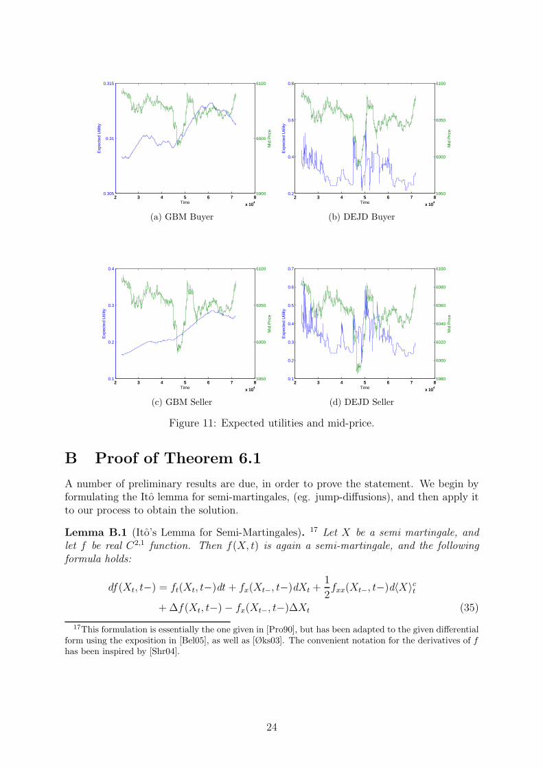
Figure 11: Expected utilities and mid-price.
B Proof of Theorem 6.1
A number of preliminary results are due, in order to prove the statement. We begin byformulating the Ito lemma for semi-martingales, (eg. jump-diffusions), and then apply itto our process to obtain the solution.
Lemma B.1 (Ito’s Lemma for Semi-Martingales). 17 Let X be a semi martingale, andlet f be real C2,1 function. Then f(X, t) is again a semi-martingale, and the followingformula holds:
df(Xt, t−) = ft(Xt, t−)dt+ fx(Xt−, t−)dXt +1
2fxx(Xt−, t−)d〈X〉ct
+∆f(Xt, t−)− fx(Xt−, t−)∆Xt (35)
17This formulation is essentially the one given in [Pro90], but has been adapted to the given differentialform using the exposition in [Bel05], as well as [Øks03]. The convenient notation for the derivatives of fhas been inspired by [Shr04].
24

with the following notations:
fx(X, t) :=∂f
∂X(X, t), ft(X, t) :=
∂f
∂t(X, t), fxx(X, t) :=
∂2f
∂X2(X, t),
t− := limǫ↓0
t− ǫ, ∆Xt := Xt −Xt−,
∆f(Xt, t−) := f(Xt, t−)− f(Xt−, t−).
Also d〈X〉ct is the differential of the quadratic variation process of the continuous part ofXt.
Proof. A proof is given in [Pro90], p. 78.
As a consequence the following corollary for the Doleans-Dade stochastic exponentialfor semi-martingales can be formulated:
Corollary B.1 (Stochastic Exponential for Semi-martingales). 18 Let Xt be a semi-martingale, X0 = 0. Then there exists a unique semi-martingale Zt satisfying dZt =Zt−dXt with Z0 = 1. Zt is given by:
Zt = exp
(Xt −
1
2〈X〉ct
)∏
s≤t
((1 + ∆Xs) exp(−∆Xs)
)(36)
Proof. Cf. [Pro90], p.84.
Proof of Theorem 6.1 . Consider the following function
f(x, t) := xeµt, fx(x, t) = eµt, fxx(x, t) = 0, ft(x, t) = µxeµt = µf(x, t).
We look for a solution of the form;
Xt = Cteµt
for some semi-martingale Ct. Applying the Ito-formula for semi-martingales we obtain:
dXt = df(Ct, t) = eµtdCt + µCteµtdt
Notice that under the assumption Xt = Cteµt the SDE can be rewritten as:
dXt = Cteµt(σdBt + dJt + µdt)
Comparing the last two equations, we conclude that:
dCt = Ct(σdBt + dJt),
and by virtue of the previous corollary, we know that the unique solution for Ct is givenby:
Ct = S exp
(σBt +
Nt∑
i=1
(Vi − 1)−1
2σ2t
)Nt∏
i=1
Vi exp(− (Vi − 1)
)
= S exp
(σBt −
1
2σ2t
) Nt∏
i=1
Vi,
18Again, this formulation has been adapted from Theorem 37 in [Pro90], p. 84 to be in the moreconvenient differential form and in the shorter form, as given in the theorem’s proof also there.
25

which yields
Xt = Cteµt = exp
((µ−
σ2
2
)t+ σBt
) Nt∏
i=1
Vi,
concluding the proof.19
Note that (18) is the same as:
St = S exp
(µ−
σ2
2
)t+ σBt +
N(t)∑
i=1
Yi
(37)
C Proof of Theorem 6.2
Definition C.1 (Poisson Process). A right-continuous process (Nt)t≥0 with state spaceN0 is a time homogeneous Poisson process with intensity rate λ iff the following is true:
a) N0 = 0 a.s.;
b) the process has stationary, independent increments, which are Poisson distributed,i.e. for all s, t ≥ 0 Ns+t −Ns ∼ Poi(λt).
Definition C.2 (Compound Poisson Process). Let (Nt)t≥0 be a time homogeneous Pois-son process with intensity rate λ and (Yn)n∈N a family of iid random variables, and let thefamily further be independent of (Nt)t≥0. The process (Ct)t≥0, defined by
Ct :=
Nt∑
i=1
Yi, t ≥ 0
is called a compound Poisson process.
Lemma C.1. For a time homogeneous compound Poisson process (Ct)t≥0 with intensityrate λ and square-integrable Y1 the following holds:
E[Ct] = λtE[Y1] and V[Ct] = λtE[Y 21
].
Proof. Cf. [MS05], Theorem 10.24, iii).
We will also need a slight variation of this Lemma concerning the moments of a“Poisson product” of iid random variables, which we will prove:
Lemma C.2. Let (Nt)t≥0 be a time homogeneous Poisson process with intensity rate λand let t ≥ 0 be fixed. Further let (Yi)i∈N be a family of iid random variables, which isalso independent of the Poisson process. Then for the “Poisson product”:
Pt :=
Nt∏
i=1
Vi (38)
19An intuitive proof of this with omission of technicalities is given in [Pol06].
26
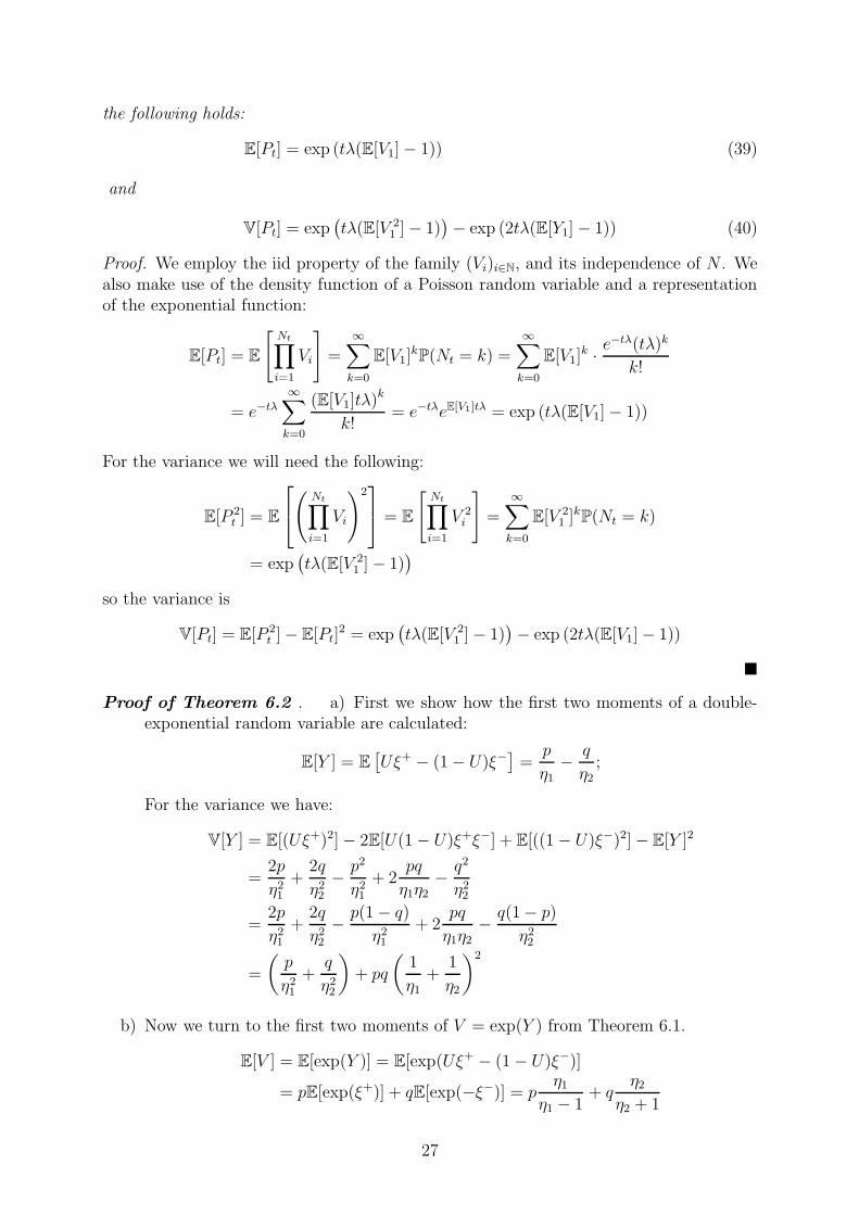
the following holds:
E[Pt] = exp (tλ(E[V1]− 1)) (39)
and
V[Pt] = exp(tλ(E[V 2
1 ]− 1))− exp (2tλ(E[Y1]− 1)) (40)
Proof. We employ the iid property of the family (Vi)i∈N, and its independence of N . Wealso make use of the density function of a Poisson random variable and a representationof the exponential function:
E[Pt] = E
[Nt∏
i=1
Vi
]=
∞∑
k=0
E[V1]kP(Nt = k) =
∞∑
k=0
E[V1]k ·
e−tλ(tλ)k
k!
= e−tλ
∞∑
k=0
(E[V1]tλ)k
k!= e−tλeE[V1]tλ = exp (tλ(E[V1]− 1))
For the variance we will need the following:
E[P 2t ] = E
(
Nt∏
i=1
Vi
)2 = E
[Nt∏
i=1
V 2i
]=
∞∑
k=0
E[V 21 ]
kP(Nt = k)
= exp(tλ(E[V 2
1 ]− 1))
so the variance is
V[Pt] = E[P 2t ]− E[Pt]
2 = exp(tλ(E[V 2
1 ]− 1))− exp (2tλ(E[V1]− 1))
Proof of Theorem 6.2 . a) First we show how the first two moments of a double-exponential random variable are calculated:
E[Y ] = E[Uξ+ − (1− U)ξ−
]=
p
η1−
q
η2;
For the variance we have:
V[Y ] = E[(Uξ+)2]− 2E[U(1− U)ξ+ξ−] + E[((1− U)ξ−)2]− E[Y ]2
=2p
η21+
2q
η22−
p2
η21+ 2
pq
η1η2−
q2
η22
=2p
η21+
2q
η22−
p(1− q)
η21+ 2
pq
η1η2−
q(1− p)
η22
=
(p
η21+
q
η22
)+ pq
(1
η1+
1
η2
)2
b) Now we turn to the first two moments of V = exp(Y ) from Theorem 6.1.
E[V ] = E[exp(Y )] = E[exp(Uξ+ − (1− U)ξ−)]
= pE[exp(ξ+)] + qE[exp(−ξ−)] = pη1
η1 − 1+ q
η2η2 + 1
27

where in the last step we used the moment generating function of the exponentialdistribution (cf. [MS05], p. 102). Note that for the first moment of V to to befinite, η1 > 1 is required, and for E[V 2] < ∞, η1 > 2 is needed (cf. [MS05], p. 103).Note that we have explicitly imposed those constraints in our model. Now we turnto the variance. First we obtain:
E[V 2] = E[exp(2Y )] = E[exp(U2ξ+ − (1− U)2ξ−)]
= pE[exp(2ξ+)] + qE[exp(−2ξ−)] = pη1
η1 − 2+ q
η2η2 + 2
,
and again, the last step was produced by using the moment generating function ofan exponential distribution. So, in summary, the variance of V is given by:
V[V ] = E[V 2]− E[V ]2
= pη1
η1 − 2+ q
η2η2 + 2
−
(p
η1η1 − 1
+ qη2
η2 + 1
)2
c) This has been considered in the previous lemma.
d) Next we turn to the moments of the stochastic process itself:
E[St] = E
S exp
((µ−
σ2
2
)t+ σBt
)N(t)∏
i=1
Vi
= SE
[exp
((µ−
σ2
2
)t + σBt
)]E
N(t)∏
i=1
Vi
= S exp(µt)E[Pt]
where Pt is the “Poisson product” from (38), and the term eµt was obtained as thefirst moment of a log-normally distributed random variable, which corresponds todistribution of the GBM process in time. Next, we look at the second moment ofthe DEJD:
E[S2t ] = E
S2 exp
(2
(µ−
σ2
2
)t+ 2σBt
)N(t)∏
i=1
V 2i
= S2 exp(2µt+ σ2t)E[P 2t ],
so in summary the variance is given by:
V[St] = E[S2t ]− E[St]
2 = S2e2µt(eσ
2tE[P 2
t ]− E[Pt]2)
e) Finally, after characterizing the process itself, we take a look at the log-returnsl(∆t), which are of particular importance for our empirical work, as we calibrateour model parameters, so as to match the rolling volatility and mean of the observed
28

log-returns in the market:
E[l(∆)] = E
log
S exp
((µ−
σ2
2
)(t+∆t) + σBt+∆t +
∑Nt+∆t
i=1 Yi
)
S exp
((µ−
σ2
2
)t) + σBt +
∑Nt
i=1 Yi
)
= E
[(µ−
σ2
2
)∆t + σB∆t +
N∆t∑
i=1
Yi
]
=
(µ−
σ2
2
)∆t + λ∆tE[Y ]
=
(µ−
σ2
2
)∆t + λ∆t
(p
η1−
q
η2
)
where the penultimate step was achieved by observing that∑N∆t
i=1 Yi is a compoundPoisson process and together with Lemma C.1.
We obtain the variance as the sum of two independent random variables, namely ascaled Brownian motion with drift and a compound Poisson process:
V [l(∆t)] = V
[(µ−
σ2
2
)∆t+ σB∆t +
N∆t∑
i=1
Yi
]
= V
[(µ−
σ2
2
)∆t + σB∆t
]+ V
[N∆t∑
i=1
Yi
]
= σ2∆t + λ∆t
(2p
η21+
2q
η22
)
29

D Descriptive Statistics
GBM DEJDBid Ask Bid Ask
Date r σr U σU r σr U σU r σr U σU r σr U σU
6/7/2010 1.6697 1.5638 0.3343 0.0534 1.2232 0.961 0.3791 0.0348 2.5968 0.4754 0.3106 0.0668 2.7041 0.4278 0.3114 0.07426/8/2010 1.7938 1.5542 0.3516 0.0011 1.9258 1.8318 0.3742 0.0197 2.5922 1.6858 0.3807 0.0553 2.4968 1.6743 0.3953 0.05736/9/2010 1.4389 1.2 0.3492 0.0012 1.4433 1.0755 0.3534 0.0149 0.4052 0.0078 0.2457 0.0134 0.3832 0.0047 0.217 0.00696/10/2010 0.8532 0.8239 0.3963 0.0462 1.8643 1.7271 0.3165 0.0465 2.0466 0.9349 0.3361 0.0583 2.1711 1.0722 0.3354 0.05346/11/2010 1.8339 1.6336 0.3107 0.0015 4.2609 4.8068 0.2276 0.0378 2.3427 0.9756 0.3203 0.0615 2.3329 0.8856 0.3259 0.07376/14/2010 6.6012 7.2139 0.1279 0.0013 1.2499 0.9366 0.3096 0.0219 0.3846 0.0061 0.2303 0.0102 0.3762 0.0063 0.2266 0.01136/15/2010 1.052 0.8965 0.3239 0.0371 2.3865 2.6579 0.2521 0.0176 0.4021 0.0025 0.2508 0.0042 0.4021 0.0025 0.2509 0.00416/16/2010 11.5236 14.185 0.072 0.0009 1.3205 1.025 0.2986 0.0145 1.6776 0.426 0.3123 0.0589 2.1813 0.7166 0.2892 0.06866/17/2010 4.262 5.6016 0.1753 0.0012 1.5435 1.6336 0.3001 0.0153 1.7524 1.1442 0.3314 0.0675 1.9127 1.3945 0.3243 0.06466/18/2010 22.2285 28.0068 0.0175 0.0093 8.8825 13.3641 0.1291 0.1044 1.5505 0.6049 0.3945 0.0918 1.1383 0.4843 0.44 0.10146/22/2010 1.4545 0.8066 0.345 0.0002 13.7943 13.4171 0.0854 0.0032 1.3359 0.4592 0.3831 0.0483 1.3734 0.4972 0.3819 0.04196/23/2010 1.3237 1.7857 0.3549 0.0451 2.9182 3.4364 0.2497 0.0179 0.4014 0.0132 0.2477 0.0222 0.4068 0.014 0.265 0.0256/24/2010 16.0602 26.9084 0.101 0.0736 13.8511 19.5797 0.0912 0.0305 0.3802 0.0095 0.231 0.0161 0.3785 0.0101 0.2302 0.0196/25/2010 4.6223 4.7647 0.211 0.0016 3.4199 3.4273 0.2549 0.0348 2.857 0.7843 0.2998 0.0671 2.5293 0.5724 0.3112 0.06256/28/2010 1.7127 1.5893 0.2786 0.0007 3.7916 3.8808 0.1966 0.0235 2.1239 0.44 0.2915 0.0527 2.0837 0.4705 0.294 0.05486/29/2010 1.2483 2.1697 0.3852 0.0123 1.4386 1.9251 0.356 0.0263 2.5392 1.9022 0.3322 0.0867 2.6234 1.9291 0.3251 0.07426/30/2010 26.0247 50.6983 0.0548 0.0136 3.0267 5.1741 0.2782 0.0227 2.5383 2.0542 0.3331 0.1372 2.5013 2.0531 0.3295 0.09937/1/2010 2.1873 2.3846 0.31 0.001 1.4374 1.1859 0.3586 0.0159 0.4077 0.006 0.2618 0.0121 0.3763 0.0037 0.2151 0.00567/2/2010 6.3956 17.3426 0.2048 0.0017 3.862 9.8311 0.2759 0.0259 3.2363 2.5481 0.3152 0.1132 3.1933 2.6095 0.3152 0.09857/5/2010 1.1382 1.5598 0.17 0.002 10.2659 19.6048 0.0237 0.0072 0.395 0.0159 0.2358 0.0368 0.3885 0.011 0.2233 0.02347/6/2010 34.3653 43.3035 0.0191 0.0013 6.8719 7.5546 0.1344 0.0144 1.7868 0.7025 0.3126 0.0542 1.7482 0.6176 0.3141 0.05547/7/2010 1.965 1.3795 0.2742 0.0217 6.6386 7.1599 0.1634 0.0323 2.2267 0.4787 0.3021 0.0498 2.5558 0.5673 0.2914 0.05277/8/2010 2.0677 1.8456 0.222 0.0005 7.5357 8.391 0.1011 0.017 1.4505 0.3396 0.3087 0.0523 1.5376 0.4038 0.2987 0.05177/9/2010 0.703 0.4733 0.3216 0.0046 1.8586 1.4371 0.2203 0.0399 1.4362 0.2944 0.2874 0.0516 1.3547 0.2469 0.2978 0.04877/12/2010 6.0655 7.8103 0.1004 0.0502 1.1233 0.8429 0.2722 0.0285 1.505 0.32 0.2861 0.0567 1.4453 0.2839 0.2841 0.0543
Figure 12: Descriptive statistics per day: r is the mean impatience rate, σr is its standard deviation, U is the expected utility and σU isits standard deviation. Notice that σr is much more lower for the DEJD.
30

GBM DEJDBid Ask Bid Ask
Date r σr U σU r σr U σU r σr U σU r σr U σU
7/13/2010 2.5726 4.5379 0.227 0.0393 11.6462 30.8123 0.0989 0.0173 1.3068 0.7884 0.3331 0.0811 1.4829 0.9567 0.3193 0.06717/14/2010 66.3458 83.8717 0.0032 0.002 2.6034 2.9797 0.2073 0.0333 0.3939 0.013 0.2296 0.0244 0.3958 0.0115 0.248 0.027/15/2010 1.7529 1.8065 0.2833 0.0445 24.0865 35.2304 0.0425 0.0097 0.3987 0.0107 0.2469 0.0158 0.3987 0.0107 0.247 0.01577/16/2010 8.1558 13.0939 0.1375 0.0016 1.5682 1.619 0.3109 0.0165 0.413 0.0138 0.2527 0.0276 0.4033 0.0123 0.2473 0.02027/19/2010 1.6708 2.1856 0.2986 0.0826 2.4383 2.9992 0.2468 0.0384 0.418 0.0337 0.2371 0.0263 0.384 0.013 0.2203 0.0247/21/2010 5.5933 10.7429 0.2368 0.1321 7.1283 8.1209 0.148 0.027 0.4117 0.0143 0.2535 0.0254 0.3862 0.0101 0.2228 0.01617/22/2010 0.7802 0.666 0.3541 0.0206 4.61 6.0582 0.1822 0.0246 0.3815 0.0089 0.227 0.016 0.383 0.0089 0.2312 0.01687/23/2010 6.9123 8.6572 0.1398 0.0012 3.4125 4.049 0.2419 0.0248 2.2171 0.7722 0.3184 0.0929 2.3033 0.8736 0.3115 0.07987/26/2010 0.6593 0.642 0.3751 0.0202 4.4491 5.443 0.1689 0.021 2.1006 0.4758 0.2792 0.0697 1.9081 0.4389 0.2903 0.06797/27/2010 7.7934 13.9949 0.1185 0.0841 6.6015 16.2536 0.174 0.102 0.3842 0.0092 0.229 0.0166 0.381 0.0075 0.2289 0.01237/28/2010 8.2239 9.3875 0.0901 0.0008 2.3513 2.2435 0.2132 0.0112 1.8266 0.3681 0.2875 0.0544 1.8567 0.383 0.2822 0.05197/29/2010 15.1407 22.151 0.0632 0.0007 2.551 2.6095 0.2452 0.017 1.6739 0.8145 0.3183 0.0613 1.8035 1.0716 0.3153 0.05928/3/2010 4.4311 6.3508 0.1277 0.0006 14.0899 30.2006 0.1576 0.1154 1.9171 0.843 0.2684 0.0686 1.916 0.7999 0.2687 0.06938/4/2010 23.3697 41.5286 0.0327 0.0004 28.1208 57.8002 0.0324 0.0062 1.5608 0.8342 0.3474 0.133 1.4836 0.7579 0.3518 0.11028/5/2010 7.3107 10.2559 0.0777 0.0194 1.9764 2.0087 0.2044 0.0081 0.4424 0.1187 0.2247 0.0164 0.3816 0.0123 0.2073 0.04848/6/2010 3.5688 8.4808 0.2822 0.1811 5.8963 23.0231 0.2299 0.0527 0.4194 0.0037 0.2666 0.0097 0.4194 0.0037 0.2666 0.00978/9/2010 0.8401 0.8582 0.261 0.0069 0.9572 1.1474 0.2637 0.0604 1.1236 0.225 0.2818 0.0529 1.1571 0.2477 0.2807 0.05788/10/2010 4.3673 10.5804 0.1972 0.0593 3.3188 5.7592 0.2232 0.0387 2.0107 0.7966 0.2951 0.0722 2.0289 0.7885 0.2953 0.06998/11/2010 1.3226 1.9279 0.3206 0.1137 1.2163 0.961 0.2964 0.0256 0.4032 0.0066 0.2551 0.0143 0.4155 0.0074 0.2665 0.01438/12/2010 1.7891 2.0906 0.2748 0.0346 3.9149 6.4365 0.2044 0.0273 0.4017 0.0083 0.2489 0.0151 0.398 0.0098 0.2452 0.02018/16/2010 1.0649 0.9926 0.3472 0.016 2.6688 3.0557 0.2455 0.0239 0.3825 0.008 0.236 0.014 0.3918 0.0077 0.2337 0.01268/17/2010 15.4901 23.2717 0.0447 0.013 2.0762 2.1442 0.2349 0.0961 0.3995 0.0062 0.2381 0.0115 0.3785 0.0032 0.2129 0.00518/18/2010 2.1794 2.4913 0.2218 0.0113 9.6789 13.3676 0.0875 0.0139 0.4078 0 0.2606 0 0.4079 0 0.2607 0.00018/19/2010 11.8686 23.3092 0.1226 0.0011 44.7998 88.3008 0.0664 0.084 2.9749 2.7303 0.3225 0.0813 3.0228 2.6258 0.3226 0.07948/20/2010 1.8464 1.7797 0.2703 0.0414 1.4503 1.5248 0.3003 0.0312 2.1296 0.8265 0.2908 0.0713 2.4249 0.8283 0.2785 0.0801
Mean 7.3128 10.6631 0.2144 0.0262 6.0309 9.8203 0.2166 0.0319 1.3374 0.5272 0.2858 0.0483 1.3501 0.537 0.2829 0.0462
Figure 13: Continued - descriptive statistics per day: r is the mean impatience rate, σr is its standard deviation, U is the expected utilityand σU is its standard deviation. Notice that σr is much more lower for the DEJD.
31

E Limit Order Book
The limit order book at a point in time
Ask sizes
Bid sizes
2.5 3.00 3.50
Mid price
4.00 4.50 5.00
Asset price
6
5
4
3
2
1
0
1
2
3
4
5
6
Figure 14: A stylized snapshot of the LOB with three levels of information at an arbitrarypoint in time. The mid-price is 3.75, and is the mid-point between the highest bid andthe lowest ask offer, which are in this case 3.50 and 4.00 respectively. The block sizesrepresent the total number of orders at each level in the book. Block sizes below theabscissa represent bid-order sizes, while above - ask-order sizes.
The limit order book (LOB) is the collection of buy and sell orders at any point intime. We will explain how it works from the perspective of a buyer. Consider the exampleof a stylized LOB given in Figure 14. There are six buy orders at a price of 2.50, two buyorders at a price of 3.00, and three orders to buy at 3.50. Note that we do not know if ateach level, the order sizes represent order submission by a single participant, or are simplyaggregated by the exchange by their limit price. For our purposes it is not important whoexactly places which orders at which level, so we can safely assume that all orders at eachlevel are placed by a single trader. Currently the best buy order is the one at 3.50 forthree shares. Assume a new buyer wants to enter the market. They could place a limitorder at 3.50 or less, but will have to wait before the current orders at 3.50 are matchedby a seller, or are cancelled by the respective buyer. They could alternatively place a limitorder between 3.50 and 4.00, thus narrowing the bid-ask spread, but declaring that they
32

are willing to pay more than the current best bid offer. This would move the indicativemid-price up. Or, lastly, they could place a market order. Assume they place a marketorder for four shares. In this scenario the two limit sell orders at four, and the two limitsell orders at 4.50 will be executed, and the order be fully filled. The outermost ask levelat 5.00 will become the best ask offer, and the mid-price will move from 3.75 to 4.25. Atlast, consider the following strategy for our hypothetical buyer, who wants to buy fourshares at a price of four. They could place a market order for two shares, which willimmediately be matched by the best ask price at 4.00, and also place a limit buy orderat 4.00 for another two shares, thus becoming the best bidder at 4.00. Notice also that inthe last scenario, the limit buy order at 2.50 will become invisible to a market participantwho only has access to the best three offers on each side of the mid-price. In exchange,potentially a new limit sell order at above 5.00 will be illuminated as the best sell ordergot filled and the participant is entitled to only see the best three sell orders.
F Empirical Fitting
In this section we first give the reader an idea of what the raw LOB data looks like,what particular type of data we have had at our avail, and what is an efficient way toorganize it for further analysis. Next, we will present our method of calibration of themodel parameters to market data and finally we describe the specificities of our fittingprocedure, with which the impatience rate is estimated.
An excerpt of raw LOB data for August 20, 2010 is given in Figure 15:The data consists of a time stamp in milliseconds, the level at which a change in the
LOB has occurred, followed by the updated bid limit price, ask limit price, bid order sizeand ask order size. Notice that the data simply gives an update at each level if somethingchanges and is in itself not the LOB. Much rather it is our task to reconstruct from thisdata set the actual snapshot of the LOB at each point in time. In the example of Figure15, the first three orders timestamped 13:59:32:367 update the order at levels three, fourand zero. Notice that level zero is designated to be the level at which the best bid andthe best ask orders are given. Thus, the spread at the beginning of this excerpt is 0.5 -the difference between 6023.5 and 6024 - which is also the tick-size, i.e. the minimal priceincrement, of the DAX future. Then, at time 13:59:32:383 updates to the levels one andtwo are seen (previous values not given in this excerpt), and an update to the ask size inlevel three - it has gone down from 32 to 30. Of particular interest is the event of orderexecution. In our example we see an order being executed at level zero at 13:59:32:397,which is indicated by a price matching of, in this case, 6024, which was the previous bestask offer. The transaction size is the lesser of the two order sizes at that level, which is onein the given example. We don’t know if it is the agent with the previous best bid offer of6023.5 who has cancelled all or part of their orders and placed a market order, or a limitbuy order at 6024, which was immediately executed. What would seem more plausiblein this case is that a new agent has come to the market, placing a market order for onefutures contract, as we can see in the follow-up update at 13:59:32:413 that there are noweven more orders at 6023.5, which are now on level one (previously zero) on the bid side,i.e. this price is no longer the best bid offer. Notice also how in the time immediatelyafter the order execution, an automatic update of levels takes place on the ask side - whatwas previously at level three, is now at level two, what was previously at level four, isnow at level three and so forth. It is unfortunate that our data does not contain orderflags, which explain exactly what has happened in each time-step, i.e. containing explicit
33

Time (ms) Level Bid Limit Ask Limit Bid size Ask size· · · · · · · · · · · · · · · · · ·
13:59:32:367; 3; 6022; 6025.5; 25; 3213:59:32:367; 4; 6021.5; 6026; 34; 4313:59:32:367; 0; 6023.5; 6024; 4; 213:59:32:383; 1; 6023; 6024.5; 14; 1213:59:32:383; 2; 6022.5; 6025; 14; 2313:59:32:383; 3; 6022; 6025.5; 25; 3013:59:32:397; 4; 6021.5; 6026; 34; 2113:59:32:397; 0; 6024; 6024; 1; 213:59:32:413; 1; 6023.5; 6024.5; 8; 1213:59:32:413; 2; 6023; 6025; 15; 2313:59:32:413; 3; 6022.5; 6025.5; 15; 3013:59:32:430; 4; 6022; 6026; 25; 2113:59:32:430; 0; 6024; 6024.5; 1; 1413:59:32:430; 1; 6023.5; 6025; 8; 2313:59:32:430; 2; 6023; 6025.5; 15; 3013:59:32:430; 3; 6022.5; 6026; 15; 2113:59:32:443; 4; 6022; 6026.5; 25; 1513:59:32:443; 3; 6022.5; 6026; 16; 2113:59:32:460; 4; 6022; 6026.5; 26; 1513:59:32:460; 0; 6024; 6024.5; 1; 1313:59:32:460; 1; 6023.5; 6025; 8; 2213:59:32:460; 3; 6022.5; 6026; 16; 2213:59:32:460; 4; 6022; 6026.5; 26; 1613:59:32:477; 0; 6024; 6024.5; 2; 1313:59:32:477; 1; 6023.5; 6025; 10; 2213:59:32:477; 4; 6022; 6026.5; 32; 1613:59:32:490; 0; 6024; 6024.5; 2; 1113:59:32:490; 2; 6023; 6025.5; 15; 2813:59:32:490; 3; 6022.5; 6026; 16; 1713:59:32:490; 4; 6022; 6026.5; 32; 1713:59:32:490; 0; 6024; 6024.5; 3; 11
· · · · · · · · · · · · · · · · · ·
Figure 15: Raw data of the nearest DAX future (FDAX) of August 20, 2010 with a depthof six levels - zero to five - on each side of the book.
information whether an order has been executed, or more interestingly since it cannotbe reliably reconstructed from this data, if an order has been cancelled. However, usinginterpretation techniques as demonstrated in the previous paragraph, one can reconstructthe LOB at each time step and have a complete picture of what the LOB looks like ateach point in time. This is also the way we organize our data for further analysis. Inorder to have a better understanding of how exactly we have reconstructed the LOB fromthe raw data, please see Appendix C, where the data from Figure 15 has been composedin a more convenient way for further analysis.
34

G Formatted LOB Snapshots
Level 0 Level 1 Level 2 Level 3 Level 4T BP AP BS AS BP AP BS AS BP AP BS AS BP AP BS AS BP AP BS AS
13:59:32:367 6023.5 6024 4 2 0 0 0 0 0 0 0 0 6022 6025.5 25 32 6021.5 6026 34 4313:59:32:383 6023.5 6024 4 2 6023 6024.5 14 12 6022.5 6025 14 23 6022 6025.5 25 30 6021.5 6026 34 4313:59:32:397 6024 6024 1 2 6023 6024.5 14 12 6022.5 6025 14 23 6022 6025.5 25 30 6021.5 6026 34 2113:59:32:413 0 0 0 0 6023.5 6024.5 8 12 6023 6025 15 23 6022.5 6025.5 15 30 6021.5 6026 34 2113:59:32:430 6024 6024.5 1 14 6023.5 6025 8 23 6023 6025.5 15 30 6022.5 6026 15 21 6022 6026 25 2113:59:32:443 6024 6024.5 1 14 6023.5 6025 8 23 6023 6025.5 15 30 6022.5 6026 16 21 6022 6026.5 25 1513:59:32:460 6024 6024.5 1 13 6023.5 6025 8 22 6023 6025.5 15 30 6022.5 6026 16 22 6022 6026.5 26 1613:59:32:477 6024 6024.5 2 13 6023.5 6025 10 22 6023 6025.5 15 30 6022.5 6026 16 22 6022 6026.5 32 1613:59:32:490 6024 6024.5 3 11 6023.5 6025 10 22 6023 6025.5 15 28 6022.5 6026 16 17 6022 6026.5 32 17
Figure 16: Consecutive LOB state snapshots, based on the example of Figure 15. FDAX 20 August, 2010. T is the time-stamp, BP andAP are respectively the bid and ask limit order prices, BS and AS are respectively the bid and ask sizes at the given level.
This is an example of how LOB is organized for further use. It is based on data from Figure 15 and shows the state of the LOB ateach point in time, whenever the LOB has been updated. It is assumed that the LOB was blank before the first time-stamp from theexcerpt in Figure 15. What follows is simply a horizontal collection of all orders with the same time-stamp. If nothing has changed at agiven level, then simply the state from the previous time step is copied. A cancellation would not be explicitly given, but would result inorders from higher levels in the LOB taking up the place of the cancelled order. If there are no orders at higher levels, then the cancelledorder would be filled with zeros. Notice that several updates per time step are possible, including changes of the level of existing orders,incoming new orders, cancellation of previous orders, changes in the price or the order size of orders at a given level, and also executionof orders by matching, or submission of a market order by a new market participant. Observe the order execution at 13:59:32:397 andhow in the next period the exchange does not quote a next best offer. Also look at how the orders from upper ask levels assume lowerlevels immediately after the execution of what appears to have been a market order at 13:59:32:397, as now the previous best bid offer of6023.5 reappears at level one, instead of level zero as the second best bid offer.
35

References
[AM10] Thierry Ane and Carole Metais, Jump Distribution Characteristics: Evidencefrom European Stock Markets, International Journal of Business and Eco-nomics 9 (2010), no. 1, 1–22.
[AS06] Marco Avellaneda and Sasha Stoikov, High-Frequency Trading In a LimitOrder Book, 2006.
[Bar10] M. Bartolozzi, A Multi Agent Model For the Limit Order Book Dynamics, TheEuropean Physical Journal B - Condensed Matter and Complex Systems 78(2010), 265–273.
[BD89] Peter J. Brockwell and Richard A. Davis, Time Series: Theory And Methods,Springer, 1989.
[BD02] , Introduction to Time Series and Forecasting, 2 ed., Springer, 2002.
[Bel05] Anatoliy Belaygorod, Solving Continuous Time Affine Jump-Diffusion Modelsfor Econometric Inference, 2005.
[BF10] Richard L. Burden and J. Douglas Faires, Numerical Analysis, 9 ed., BrooksCole, 2010.
[BMP02] Jean-Philippe Bouchaud, Marc Mezard, and Marc Potters, Statistical Proper-ties of Stock Order Books: Empirical Results And Models, Science & Finance(CFM) working paper archive 0203511, Science & Finance, Capital Fund Man-agement, 2002.
[BNS04] Ole E. Barndorff-Nielsen and Neil Shephard, Power and Bipower Varia-tion with Stochastic Volatility and Jumps, Journal of Financial Econometrics(2004).
[Bro09] Peter J. Brockwell, An Overview of Asset-Price Models, Handbook of Finan-cial Time Series, Springer, 2009, pp. 403–419.
[BS96] Andrei N. Borodin and Paavo Salminen, Handbook of Brownian Motion -Facts and Formulae, Birkhauser Verlag, 1996.
[CKS10] Rama Cont, Arseniy Kukanov, and Sasha Stoikov, The Price Impact of OrderBook Events, SSRN eLibrary (2010).
[CST08] Rama Cont, Sasha Stoikov, and Rishi Talreja, A Stochastic Model for OrderBook Dynamics, SSRN eLibrary (2008).
[Der03] Emanuel Derman, Laughter in the Dark - the Problem of the Volatility Smile,2003.
[EKL07] Zoltan Eisler, Janos Kertesz, and Fabrizio Lillo, The Limit Order Book onDifferent Time Scales, Quantitative finance papers, arXiv.org, 2007.
[Gat10] Jim Gatheral, Jump-Diffusion Models, Encyclopedia of Quantitative Finance(Rama Cont, ed.), Wiley, 2010.
36

[GPW+10] Martin D. Gould, Mason A. Porter, Stacy Williams, Mark McDonald,Daniel J. Fenn, and Sam D. Howison, The Limit Order Book: A Survey,arXiv:1012.0349v1 (2010).
[Jai03] Pankaj K. Jain, Institutional Design and Liquidity at Stock Exchanges aroundthe World, SSRN eLibrary (2003).
[JKZ09] Ken Jackson, Alexander Kreinin, and Wanhe Zhang, Randomization in theFirst Hitting Time Problem, Statistics & Probability Letters 79 (2009), no. 23,2422–2428.
[JYC09] Monique Jeanblanc, Marc Yor, and Marc Chesney, Matehmatical Methods forFinancial Markets, Springer, 2009.
[Kle06] Achim Klenke, Wahrscheinlichkeitstheorie, Springer, 2006.
[Kou02] S. G. Kou, A Jump-Diffusion Model for Option Pricing, Management Science48 (2002), no. 8, 1086–1101.
[KS89] I. Karatzas and St. E. Shreve, Brownian motion and stochastic calculus,Springer, 1989.
[KW03] S. G. Kou and Hui Wang, First Passage Times of a Jump Diffusion Process,Advanced Applied Probability 35 (2003), 504–531.
[MFE05] Alexander J. McNeil, R’udiger Frey, and Paul Embrechts, Quantitative RiskManagement: Concepts, Techniques and Tools, Princeton University Press,2005.
[MLMK08] Koichi Maekawaa, Sangyeol Leeb, Takayuki Morimotoc, and Ken-ichi Kawaid,Jump Diffusion Model With Application to the Japanese Stock Market, Math-ematics and Computers in Simulation 78 (2008), no. 2-3, 223 – 236.
[MS05] David Meintrup and Stefan Schaffler, Stochastik - Theorie und Anwendungen,Statistik und Ihre Anwendungen, Springer, 2005.
[Øks03] Bernt Øksendal, Stochastic Differential Equations. An Introduction with Ap-plications, Springer, 2003.
[Pol06] Mathew Pollard, Stat 251 Paper Review: ”A Jump Diffusion Model for OptionPricing” by S.G. Kou, 2006.
[Pro90] Philip E. Protter, Stochastic Integration and Differential Equations: a NewApproach, Springer, 1990.
[PV08] Roberto Pascual and David Veredas, What Pieces of Limit Order Book Infor-mation Matter in Explaining Order Choice by Patient and Impatient Traders?,SSRN eLibrary (2008) (English).
[Ran04] Angelo Ranaldo, Order Aggressiveness in Limit Order Book Markets.
[Ros08] Ioanid Rosu, A Dynamic Model of the Limit Order Book, Review of FinancialStudies 22 (2008), 4601–4641.
37
[Ros10] , Liquidity and Information in Order Driven Markets, SSRN eLibrary(2010).
[RZ04] Cyrus A. Ramezani and Yong Zeng, An Empirical Assessment of the DoubleExponential Jump-Diffusion Process, SSRN eLibrary (2004).
[Shr04] Steven Shreve, Stochastic Calculus for Finance II: Continuous-Time Models,Springer, 2004.
[SP99] K. Ronnie Sircar and George C. Papanicolaou, Stochastic Volatility, Smile &Asymptotics, Applied Mathematical Finance 6 (1999), no. 2, 107–145.
[TB94] Peter Ter Berg, Deductibles and the Inverse Gaussian Distribution, ASTINBulletin 24 (1994), no. 2, 319–323.
[TKF09] B. Toth, J. Kertesz, and J. D. Farmer, Studies of the limit order book aroundlarge price changes, The European Physical Journal B - Condensed Matterand Complex Systems 71 (2009), 499–510.
38

0 0.5 1 1.5 2 2.5 3 3.5 40
1
2
3
4
5
6
D = Distance−to−Fill
r =
Impa
tienc
e R
ate

2 3 4 5 6 7 8
x 104
0
1
2
3
4
5
6
Impa
tienc
e R
ate
Time2 3 4 5 6 7 8
x 104
5980
6000
6020
6040
6060
6080
6100
Mid
Pric
e

2 3 4 5 6 7 8
x 104
0
10
20
Impa
tienc
e R
ate
Time2 3 4 5 6 7 8
x 104
5900
6000
6100
Mid
Pric
e