STOCHASTIC INDEX NUMBERS:

A REVIEW*

by

Kenneth W Clements School of Economics and Commerce The University of Western Australia

H Y Izan School of Economics and Commerce, and

Faculty of Economics and Commerce The University of Western Australia

and

E Antony Selvanathan School of International Business

Griffith University

Abstract

The stochastic approach is a new way of viewing index numbers in which uncertainty and statistical ideas play a central role. Rather than just providing a single number for the rate of inflation, the stochastic approach provides the whole probability distribution of inflation. This paper reviews the key elements of the approach and then discusses some previously overlooked links with Fisher’s early work contained in his book The Making of Index Numbers. We then consider some more recent developments, including Diewert’s well-known critique of the stochastic approach, and provide responses to his criticisms. We also provide a review of Theil’s work on the stochastic approach, and present and extend Diewert’s work on this topic within the context of the Country Product Dummy method which measures price levels internationally.

* We would like to acknowledge the research assistance of Mei Han and Stéphane Verani, as well as useful comments from James Fogarty, Yihui Lan and George Verikios. This research was supported in part by the ARC.

1

1. Introduction

There are two major streams in index-number theory. The first is the test approach whereby

indexes are judged on their ability to satisfy certain criteria; this stream is associated with Fisher

(1927) in particular.1 The economic theory of index numbers is the second stream and this deals

with their foundations in utility theory; for a review, see Diewert (1981). A less well known

methodology, but one which is now attracting considerable attention, is the stochastic approach

(SA). When applied to the prices, the SA to index numbers treats the underlying (or “true”) rate of

inflation as an unknown parameter to be estimated from the individual prices. That is, the

individual prices are observed with error and the problem is a signal-extraction one of how to

combine noisy prices so as to minimise the effects of measurement errors. Under certain

circumstances, this approach leads to familiar index-number formulae such as Divisia, Lasypeyres

etc., but, as uncertainty plays a key role in the SA, their foundations differ markedly from the

conventional deterministic approach. The SA provides not only a point estimate of the rate of

inflation, but also its variance, the source of which is the divergence of the individual prices from a

common trend, that is, the extent to which the structure of relative prices changes. Accordingly, the

SA provides the intuitively plausible result that it is more difficult to obtain precise estimates of

inflation when there are large changes in relative prices.

Krugman (1999) has likened the US inflationary process in the 1970s to the noise level in a

restaurant:

“Once upon a time, … the US economy was like a trendy restaurant – one of those places where the tables are set close together and the ceiling seems custom-designed to maximise the din. What happens in that kind of environment is that everyone tries to talk above the background noise so as to be heard by his or her companions. But by talking louder, you yourself raise the noise level, forcing everyone else to talk louder, raising the noise level still further, and eventually everyone is shouting themselves hoarse. Substitute wage and price increases for speaking volume and inflation for the overall noise level, and you have a capsule analysis of the kind of inflationary spiral that the US faced in the 1970s.”

Although this instructive metaphor relates to the dynamics of inflation characterised by a wage-

price spiral, it could equally well apply to the signal-extraction approach to measuring inflation.

The conversation volume at an individual table is made up of some audible words which convey an

intelligible message (the signal), plus some yelling (the noise) which does not. The measurement of

the information content of all the messages in the restaurant then involves some form of filtering to

minimise the distortive effects of the noise. This is exactly the basis of the SA in its decomposition

1 Balk (1995) provides a comprehensive survey of the test approach.

2

of the individual price changes into inflationary and relative-price components with some form of

averaging procedure filtering out the distortionary impact of the latter.

The SA is also relevant to the conduct of monetary policy and inflation targeting in

particular. A popular approach is for policy makers to exclude from the index the prices of volatile

items such as food and energy, and use “core” or “underlying” inflation for the specification of

inflation targets.2 In an another approach, the Reserve Bank of Australia currently has a “soft”

inflation target of 2-3 percent p.a. on average over the cycle. Both the exclusion of noisy prices

from the index and the idea of a soft target could be given more satisfactory statistical foundations

by employing the SA. The SA gives specific guidance regarding the weighting scheme employed

in the index; such a scheme is comprehensive in that it deals with all items in the regime, rather than

just setting to zero the weights of the volatile items. Regarding the specification of a soft target, the

SA could be used to express the target as X percent ± 1.96 standard errors, for example.

The SA originated in the work of Jevons and Edgeworth (see Frisch, 1936, for references),

but then fell into obscurity, perhaps in part due to the criticism by Keynes (1930, pp. 85-88) that it

was too rigid as the approach made no allowance for sustained changes in relative prices. For a

history-of-thought review of stochastic index numbers, see Aldrich (1992) who attributes the

introduction of the term “stochastic” in this context to Frisch (1936), and adopted by Allen (1975),

to describe Edgeworth’s analysis. More recently, the SA has been rehabilitated by Balk (1980),

Clements and Izan (1981, 1987), Crompton (2000), Giles and McCann (1994), Miller (1984),

Ogwang (1995), Ong et al. (1999), Prasada Rao and Selvanathan (1992a, b), Prasada Rao et al.

(2003), Selvanathan (1989, 1991, 1993) and Selvanathan and Prasado Rao (1992). This literature is

still expanding and has been the subject of a book by Selvanathan and Prasada Rao (1994), who

emphasise the versatility and usefulness of the approach, a review paper by Diewert (1995), which

has a critical tone, and a response by Selvanathan and Prasada Rao (1999). Even more recently,

papers have appeared by Diewert (2002, 2004) and Prasada Rao (2004) which extend the SA in new

directions.

The above-mentioned critique by Diewert (1995), while unpublished, has been influential

and widely cited as providing what some may see as a telling case against stochastic index numbers.

In this paper, we provide an in-depth assessment of the criticisms and show how the majority can be

answered satisfactorily. Section 2 of the paper provides an overview of stochastic index numbers,

while Section 3 discusses some early ideas of Fisher (1927) that seem not to have been previously

appreciated as having relevance to the stochastic approach. Our responses to Diewert’s criticisms

are contained in Section 4. Theil’s (1967) stochastic approach is presented in Section 5. Section 6 2 Related approaches involve using the median, other “trimmed” means, a dynamic factor index and averaging over longer horizons. See Bryan and Cecchetti (1993, 1994), Bryan et al. (1997) and Cecchetti (1997).

3

reviews and extends some recent results of Diewert (2002) which apply stochastic index number

theory to the problem of the measurement of price levels across countries. Concluding comments

are contained in Section 7.

2. What are Stochastic Index Numbers?

In this section, we provide a brief review of some of the basic results on stochastic index

numbers; this material is mainly based on Clements and Izan (1987). To make the exposition as

sharp and as clear as possible, we concentrate on the simplest possible cases. Although we only

consider prices, it should be clear that the SA applies also to quantities.

Let it it it 1Dp log p log p −= − be the log-change in the price of commodity i (i = 1,…, n)

from year t-1 to t. Suppose that each price change is made up of a systematic part that is common

to all prices, tα , and a zero-mean random component εit ,

(2.1) it t itDp = α + ε .

As the term αt equals E(Dpit), it is interpreted as the common trend in all prices, or the underlying

rate of inflation. With this interpretation, the change in the relative price of good i is then

it tDp − α . As equation (2.1) implies that it t itDp − α = ε and as itE ( ) 0ε = , it follows that the

expected value of the change in the ith relative price is zero, which means that, on average, all

relative prices are constant. While this is obviously restrictive, the approach can be extended by

adding a commodity-specific parameter to (2.1), as will be discussed below.

Let the disturbances in (2.1) for i, j=1,…,n, εit , have variances and covariances of the form

σijt and let t ijt = σ Σ be the corresponding n × n covariance matrix. We write (2.1) for i = 1,

…, n in vector form as

(2.2) t t t= α +Dp ι ε ,

where [ ]t itDp=Dp , [ ]1,...,1 ′=ι , and [ ]t it= εε are all n 1× vectors. Application of GLS to

(2.2) yields the BLUE of tα ,

(2.3) ( ) 11 1t t t tˆ

−− −′ ′α = ι Σ ι ι Σ Dp

with

4

(2.4) ( ) 11t tˆvar

−−′α = ι Σ ι .

As indicated above, εit is interpreted as the change in the ith relative price. Suppose that

εit and εjt for i ≠ j are independent and that the variance of εit is inversely proportional to the

corresponding budget share wit ,

(2.5) 2t

itit

varwλ

ε = ,

where λt is a parameter independent of i ; and it it it tw p q / M= is the ith budget share, with qit

the quantity consumed of good i in year t and ni 1t it itM p q=∑= total expenditure. There are two

justifications for specification (2.5), at least as an approximation: (i) As a commodity absorbs a

large part of the overall economy (i.e., as its budget share rises), there is less scope for its relative

price to vary as there is simply less amount of “all other goods” against which its price can change.

This restriction on the scope for the relative price changes of a large good means that its variance is

smaller. (ii) If we think in terms of optimal sampling of prices, it would make sense for the relevant

statistical collection agency to devote more resources to sampling prices of the more “important”

goods by obtaining more price quotations. One way of identifying the importance of a good is by

the size of its budget share. Such a sampling procedure would again lead to smaller variances of the

relative prices of the more important goods. Finally, note that as 2ni 1 it it tw var n=∑ ε = λ , the

parameter 2tλ is interpreted as proportional to a budget-share-weighted variance; this 2

tλ can also

be expressed as 2ni 1 it itw var=∑ ε .

The above assumptions imply that 2it jt ij t itcov( , ) / wε ε = δ λ , where δij is the Kronecker

delta (δij = 1 if i = j , 0 otherwise), so that the nn × covariance matrix takes the form

(2.6) 2 1t t t

−= λΣ W

where t 1t ntdiag[ w , ... , w ]=W . Equation (2.3) then becomes ( ) 1t t t tˆ −′ ′α = ι W ι ι W Dp .

Since ni 1t itw 1=∑′ = =ι W ι and n

i 1t t it itw Dp=∑′ =ι W Dp , the above simplifies to

(2.7) n

t it iti 1ˆ w Dp

=α = Σ .

5

In words, the estimator of the underlying rate of inflation is a budget-share weighted average of the

n price log-changes, an attractively simple result. In this index, more weight is given to those

goods occupying a larger fraction of the consumer’s budget, which makes intuitive sense.

Furthermore, if we reinterpret wit as the arithmetic average of the observed budget shares in years

t-1 and t, the right-hand-side of (2.7) is the Divisia price index number, which has a number of

desirable properties.3

The Divisia index is a weighted first-order moment of the n price-changes 1t ntDp , ... , Dp .

The corresponding second-order moment is the Divisia variance,

n

2t it it ti 1

w (Dp DP )=

Π = Σ − ,

where nt i 1 it itDP w Dp== Σ is the Divisia index. This variance measures the cross-commodity

variance of relative prices; when all relative prices are unchanged, tΠ 0= . Under covariance

specification (2.6), the variance of tα̂ , defined in equation (2.4), becomes ( ) 12 2t t

−′λ = λtι W ι ,

which can be estimated unbiasedly by

[ ]( ) ( ) [ ] n 2t t t t t ti 1 it itˆ ˆ1/(n 1) 1/(n 1) w (Dp DP )=

′− − α − α = − Σ −Dp ι W Dp ι , which is proportional

to the Divisia variance tΠ . Accordingly, under (2.6) we have

(2.8) t t1ˆvar

n 1α = Π

− .

In words, the sampling variance of the inflation estimator is proportional to the variance of relative

prices. When there is more dispersion of relative prices, i.e., when prices are changing more

disproportionately, the sampling variance increases. This is also an attractive result which agrees

with the intuitive idea that the underlying rate of inflation is in some sense less well defined when

there are large changes in relative prices.

The above results can be extended to allow for more general specifications for

the distribution of the disturbance terms. Crompton (2000) analyses White (1980)-type

heteroscedasticity and derives analytical scalar expressions for the standard error of inflation under

this formulation. Selvanathan and Prasada Rao (1999) consider a more general error covariance

structure. Even with these extensions, the basic insight remains unchanged, viz., the standard error

3 This is also known as the Törnqvist (1936)-Theil (1967) index.

6

of the estimate of the rate of inflation increases with the degree of variability of relative prices.

Model (2.1) can also be extended to allow for relative price changes by adding a commodity-

specific parameter iβ :

(2.9) it t i itDp = α + β + ε , itE( ) 0ε = , 2it t ivar wε = λ ,

where iw is the sample mean of itw . The new parameter iβ is interpreted as the systematic part

of the change in the ith relative price, it tDp − α . As the iβ are not identified, Clements and Izan

(1987) use the normalization that a budget-share-weighted average of the relative price changes is

zero, ni 1 i iw 0=∑ β = .

The above presentation of the key elements of the SA has been in the context of a price

index formulated in terms of changes over time. However, this is not essential as the SA is also

equally applicable to indexes in levels, such as Laspeyers and Paasche. For details, see Selvanathan

(1991, 1993) and Selvanathan and Prasada Rao (1994); also the recent results of Diewert (2002),

considered in detail in Section 6, which show how the approach can be applied to yield a number of

familiar index formulae in the context of the measurement of price levels across countries.4

3. Irving Fisher and Stochastic Index Numbers In his monumental book The Making of Index Numbers, Fisher (1927) introduced the

“atomistic” or “test” approach to index-number theory. According to this approach, the quality of a

particular index number is assessed by its ability to satisfy three primary tests. (i) The commodity-

reversal test, which means that the value of the index should be invariant to an interchange (or

reversal) in the order of any two commodities. (ii) The time-reversal test, whereby the price index

at time t with base-period 0, toP , should be the reciprocal of otP , the index at time 0 with base-

period t. In other words, the product of the forward and backward indexes should be unity. (iii)

The factor-reversal test, according to which the product of the price and quantity indexes should

equal the observable ratio of values in the corresponding years. Tests (ii) and (iii) constitute “the

two legs on which index numbers can be made to walk” (Fisher, 1927, p. xiii). One of the few

indexes that satisfied the three criteria was the geometric mean of the Laspeyres and Paasche

indexes, which came to be known as “Fisher’s ideal index”. Although Fisher’s name is not usually

associated with the stochastic approach to index numbers, a rereading of his book reveals some

4 For other cross-country applications of the SA, see Selvanathan and Prasada Rao (1992).

7

early contributions that are at least related to the approach, and can be thought of as providing some

early clues and directions. This is perhaps not surprising given the breadth and depth of this

influential book, which still commands a leading position in an area that has expanded enormously

since Fisher’s time. In what follows, these early contributions are set out.

As discussed in the previous section, the stochastic approach emphasises the idea of index

numbers as averages of the underlying component prices. Fisher also made this emphasis, as is

clear from the following (Fisher, 1927, p. 2):

There would be no difficulty … if all prices moved up in perfect unison or down in perfect unison. But since, in actual fact, the prices of different articles move very differently, we must employ some sort of compromise or average of their divergent movements.

If we look at prices as starting at any time from the same point, they seem to scatter or disperse like the fragments of a bursting shell. But, just as there is a definite centre of gravity of the shell fragments, as they move, so is there a definite average movement of the scattering prices. This average is the “index number.” Moreover, just as the center of gravity is often convenient to use in physics instead of a list of the individual shell fragments, so the average of the price movements, called their index number, is often convenient to use in economics.

An index number of prices, then, shows the average percentage change of prices from one point of time to another. The percentage change in the price of a single commodity from one time to another is, of course, found by dividing its price at the second time by its price at the first time. The ratio between these two prices is called the price relative of that one particular commodity in relation to those two particular times. An index number of the prices of a number of commodities is an average of their price relatives. (Fisher’s emphasis.)

The idea of using an index number to summarise the disparate movements in individual prices is

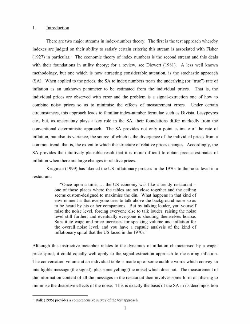
also implicit in many of Fisher’s diagrams. Figure 1 provides an example in the form of a time-

series plot of the 36 prices used by Fisher to illustrate the workings of 100+ types of indexes later in

his book. In commenting on Figure 1, and its quantity counterpart, Fisher (1927, p. 14) in fact uses

the language of the stochastic approach whereby the estimated rate of inflation (the change in the

price index) is referred to as the “common trend” in prices:

How it is possible to find a common trend for such widely scattered price relatives or quantity relatives? Will not there be as many answers to such a question as there are methods of calculation? Will not these answers vary among themselves 50 percent or 100 percent? The present investigation will show how mistaken is such a first impression.

8

Figure 1

Source: Fisher (1927, p. 12). The term “bias” is used in statistics to refer to the difference between the excepted value of

a sample statistic and its population counterpart. Fisher, however, uses the term to refer to

something different: The deviation of a given index from the time- and factor– reversal criteria.

Fisher (1927, pp. 108-9, 387-95) shows that his bias increases with the degree of dispersion of the

underlying prices and quantities. Interestingly, this is reminiscent of one of the basic results of the

stochastic approach whereby the uncertainty of the estimated rate of inflation is proportional to the

standard deviation of relative prices; see equation (2.8) above, for example. Thus under the

stochastic approach the overall rate of inflation in estimated less precisely in those periods when

there is high variability of relative prices.

9

A further link with the stochastic approach is what Fisher calls the “probable error”

involved in an index number. This seems to be Fisher’s response to the then-current criticism of

index numbers as being unreliable. A flavour of this criticism is given in the opening paragraph of

his book (Fisher, 1927, p. 1):

In 1896, in the Economic Journal, the Dutch economist, N. G. Pierson, after pointing out some apparently absurd results of index numbers, said: “The only possible conclusion seems to be that all attempts to calculate and represent average movements of prices, either by index numbers or otherwise, ought to be abandoned.” No economist would today express such an extreme view. And yet there lingers a doubt as to the accuracy and reliability of index numbers as a means of measuring price movement.

The term “probable error” is related to the sampling distribution of the mean, which can be

explained as follows. Suppose a random variable x is normally distributed with mean µ and

standard deviation σ . The probability of drawing a value of x that falls within the range

.6745µ ± × σ is then 50 percent. The quantity .6745×σ is known as the probable error in

measuring x; in other words, under normality, there is a chance of 1 in 2 of x being .6745

standard deviations away from the mean. Next, we interpret x as the sample mean of n

underlying observations 1 nx ,..., x with standard deviation [ ] n 2

i 1 i1 /(n 1) (x x)s .=

= − ∑ − Then the

standard error of the mean is s / n , which is an estimator of σ above. Accordingly, the probable

error of the mean is .6745 s / n.×

Fisher (1927, pp. 225-29) used his n 13= most preferred indexes for the period 1914-18 to

compute their probable errors. Take as an example 1917, the year in which the probable error of

the price indexes is largest at 0.128 percent. This error is to be compared to the value of the ideal

price index (identified by Fisher as “Formula Number 353”) of 161.56, so that on average prices in

1917 were 61.6 percent higher than in 1913. The 50-percent confidence interval for this year is

then 161.56 0.128± percent, or 161.35-161.77. Fisher (p. 228) was obviously excited by this

incredibly low error in declaring “[w]e may, therefore, be assured that Formula 353… is able to

correctly to measure the general trend in 36 dispersing relative prices… within less than one eighth

of one percent!...[This error] is less than three ounces on a man’s weight…” Fisher (p. 229)

concludes triumphantly by writing: “As physicists or astronomers would say, the ‘instrumental

error’ negligible. The old idea that among the difficulties in measuring price movements is the

difficulty of finding a trustworthy mathematical method may now be dismissed once and for all.”

A skeptical assessment of the above approach is that the small error simply reflects the

closeness of the 13 indexes considered. These indexes are all computed from exactly the same

underlying data and, it could be argued, the differences in the algebraic forms of the indexes are

10

relatively minor as they all involve a geometric mean of one form or another. Indeed, in at least

two cases, the index is defined as the geometric mean of two other indexes included in the list of

13.5 Nevertheless, it is clear that Fisher did have considerable early insights into the nature of the

uncertainties associated with index numbers, a topic that is central to the stochastic approach. As

mentioned above, in referring to the index value as the “common trend” in prices, Fisher himself

thought of the index as the mean of the underlying price relatives. Accordingly, had Fisher applied

probable error theory to the index itself, rather than the mean of the 13 different indexes, he would

then have identified the estimation uncertainty of the index as reflecting the degree of relative price

variability, and thus possibly been a major contributor to the development of the stochastic

approach.6

Diewert (1995) has also commented on Fisher’s attempt to assess the precision of a price

index. He points out that (Diewert, 1995, p. 22-23)

…the proponents of the test and economic approaches to index number theory use their favorite index number formula and thus provide a precise answer whether the price relatives are widely dispersed or not. Thus the test and economic approaches give a false sense of precision.

The early pioneers of the test approach addressed the above criticism. Their method works as follows: (i) decide on a list of desirable tests that an index number formula should satisfy; (ii) find some specific formulae that satisfy these tests (if possible); (iii) evaluate the chosen formulae with the data on hand and (iv) table some measure of the dispersion of the resulting index number computations (usually the range or standard deviation was chosen). The resulting measure of dispersion can be regarded as a measure of functional form error.

Diewert then goes on to describe Fisher’s application of this approach, as discussed above. Diewert

also cites the work of Persons (1928) and Walsh (1921) who apply similar methods to assessing the

reliability of price indices. Diewert (1995, p. 24) is not satisfied with the above approach and

writes:

It is clear that there are some problems in implementing the above test approach to the determination of functional form error; i.e., what tests should we use and how many index number formulae should be evaluated in order to calculate the measure of dispersion? However, it is interesting to note that virtually all the above index number formulae suggested by Fisher, Persons and Walsh approximate each other to the second order around an equal price and quantity point.

5 In Fisher’s Table 26 (p. 226) Formula Number 5307 is the geometric of Formulae 307 and 309; and 5323 323 325.= × For details, see Fisher (1927, Appendix V). 6 According to Stigler (1982), Jevons (1884, p. 157) attempted such an application but he “seems to have put only a rough faith in that result and did not repeat the attempt” (Stigler, 1982).

11

Note that the criticism implied in the last sentence of this quotation is another way of stating that the

various formulae being compared have similar structure, which is almost the same as our point

above that Fisher compared 13 geometric means of one form or another. In the subsequent section

we shall return to Diewert (1995) and discuss his criticism of the stochastic approach in detail.

Model (2.9) draws a sharp distinction between a change in the price level ( tα ) and a

change in a relative price ( iβ ). As they “wash out” in the aggregate ( i i iW 0β =Σ ), relative price

changes are not inflationary. Fisher also advocated such a distinction as a way to avoid circular

reasoning and to enhance clear thinking about the causes of inflation, as is illustrated by the

following quotation (Fisher, 1920, p. 73):

It is true that individual prices do react on one another in thousands of ways. But the several pushes and pulls among individual prices are not what raise them as a group. Such forces within the group could not move the group itself any more than a man can raise himself from the ground by tugging at his boot-straps. We cannot explain the rise or fall of a raft on the ocean by observing how one log in the raft is linked to the others and is pulled up or down by them. It is true that some prices rise more promptly than others and give the proximate reason for raising the others. The whole raft of prices is bound together and its parts creak and groan to make the needed adjustments. But such readjustments between prices do not explain why the whole raft of prices has risen. (Fisher’s emphasis.)

4. The Diewert Critique

The stochastic approach has attracted the attention of Erwin Diewert, a leading expert in

index numbers. In a major review paper, Diewert (1995) places the SA in historical context in a

masterful fashion and cites the early work on the topic by Bowley, Edgeworth and Jevons in

particular. He then goes on to make four specific criticisms of the SA in its modern version; below

we discuss each in turn.7

Criticism 1: The Variance Assumptions are not Consistent with the Facts

We return to the basic model given by equation (2.1) and note that the error term itε is

interpreted as the change in the ith relative price. Equation (2.5) postulates that the variances of

relative prices are inversely proportional to the corresponding budget shares. Accordingly, the

prices of those commodities that are more (less) important in the consumer’s budget are less (more)

variable. Diewert argues that this assumption does not agree with the observed behaviour of prices.

In support of his position, Diewert cites the evidence presented in Clements and Izan (1987, p. 345)

who conceded the point. Diewert (1995, pp.15-16) also argues:

7 For an earlier response to Diewert’s criticisms, see Selvanathan and Prasada Rao (1999).

12

…[F]ormal statistical tests are not required to support the common observation that the food and energy components of the consumer price index are more volatile than many of the remaining components. Food has a big share while energy has a small share… volatility of price components is simply not highly correlated with the corresponding expenditure shares.

While the arguments presented below equation (2.5) supporting the idea that the variance

specification (2.5) is not totally implausible,8 as indicated above the results of Clements and Izan

(1987) reject this specification. Such a rejection does not mean that the entire SA has to be

abandoned however, as this particular variance specification is only one of a multitude of

possibilities. That is to say, variance specification (2.5) is just one way of parametrising the nn ×

covariance matrix tΣ in the general expression for the variability of the index, equation (2.4). Put

slightly differently, result (2.8) is a case of the general result (2.4); the special case is based on

assumption (2.5)

To illustrate how the SA is able to deal with difference specifications of tΣ , consider three

other special cases. First, suppose the n prices are independent so that tΣ is a diagonal matrix

with 11t nnt,...,σ σ on the main diagonal. To set out the implications of this case, let t1

iitit Sx −σ= ,

where n 1t iiti 1

S −=

= σ∑ . Application of equations (2.3) and (2.4) then yields

(4.1) n

t it iti 1

ˆ x Dp=

α = ∑ , 1t tˆvar S−α = .

Here we see that the estimated rate of inflation is still a weighted average of the n price changes,

but now the weights are itx , which are proportional to the reciprocals of the variances of the

respective relative prices 1iit−σ . By construction, the weights itx are all positive fractions and have

a unit sum. Accordingly, more weight in the price index is accorded to lower variance prices,

which is a sensible property. The second member of equation (4.1) reveals that the variance of the

price index equals the inverse of tS , the sum of the reciprocals of the n variances nntt11 ,...,σσ .

As the term tS is an inverse measure of noise in the system, it follows that when there is more

8 Diewert (1995, footnote 10) thinks that Edgeworth was probably the first to make such an argument, as is revealed by the following quotation (Edgeworth, 1887, p. 247):

Each price which enters into our formula is to be regarded as the mean of several prices, which may vary with the differences of time, of place, and of quality; by the mere friction of the market, and, in the case of ‘declared values’, through errors of estimation, it is reasonable to support that this heterogeneity is greater the larger the volume of transactions.

13

variability in relative prices, 1tS− is larger, and the price index is estimated with less precision.9 In

other words, at times when prices move in a highly disproportionate manner, the overall rate of

inflation is less well defined conceptually and this is reflected in the higher estimation uncertainty

in its measurement. Again, this is a sensible property. The above example is Diewert’s (1995) neo-

Edgeworthian model, with some minor modifications.10

As a second example, suppose that at time t relative prices have a common variance 2tσ

and a common correlation coefficient tρ , so that the covariance matrix now takes the form

2t t t t[(1 ) ]′= σ − ρ + ρΣ I ιι , where I is an identity matrix and ι is an n-vector of unit elements.

Application of equations (2.3) and (2.4), as before, yields

(4.2) n

t iti 1

1ˆ Dpn =

∑α = , 2 tt t t

1ˆvarn

− ρ α = σ ρ + .

Result (4.2) shows that in the equicorrelated case, the estimated rate of inflation is an unweighted

average of the price changes, while its variance is increasing in the correlation tρ . If prices are

independent t 0ρ = and 2t tˆvar nα = σ , while if they are perfectly correlated 2

t tˆvar α = σ .

The final example is a mixture of the two specifications of tΣ considered above. For ease

of notation, we drop the t subscript from ij[ ]= σΣ , and write it as = +Σ D(I λ)D , where D is

a diagonal matrix with the standard deviation of the n prices on the matrix diagonal, 1/ 2 1/ 211 nn,...,σ σ ;

and ij[λ ]=λ is an n n× symmetric matrix with diagonal elements zero and with th(i, j) off-

diagonal element the relevant correlation, ij ij ii jjλ = σ σ σ . Recall the result that

1 ...−− = + + + ≈ +2(I λ) I λ λ I λ , if the elements of λ are not “too large”. The approximation 1−− ≈ +(I λ) I λ implies that 1 ( )−+ ≈ −(I λ) I λ , so that

(4.3) 1 1 1− − −≈ −Σ D (I λ)D .

9 Note that 1

tS− is proportional (with factor of proportionality 1/n) to the harmonic mean of 11t nnt,...,σ σ , and tS is proportional to the mean of 1 1

11t nnt,...,− −σ σ . 10 Note that in the above as the variance are time dependent, there are a large number of unknown parameters. To apply this approach in practice it would be necessary to restrict the evolution of the variances by, for example, setting

iit t ii′σ = φ σ , where tφ are parameters that are independent of commodities and ii′σ are constants. Here at certain times all variances are higher, while at other times they are all lower. The weights in the index (4.1) now become constants equal to 1 1

i ii j jjx ( ) ( )− −′ ′ ′= σ Σ σ , and 1t j jjˆvar ( )−′α = φ Σ σ .

14

This inverse has the useful property that it can be expressed as the sum of two parts, (i) a variance

component, 1 1 1ii[ ]− − −= σD D ; and (ii) a component related to the covariances,

1 1 1/ 2 1/ 2ii ij jj ij ii jj

− − − − − = − σ λ σ = − σ σ σ D λD , which is a measure of the lack of independence

among the n prices.

Define *λ as the n n× matrix 1 1− −D λD , with th(i, j) element *ijλ , and * *n

i 1j ijλ λ=∑=i as the

sum of the elements in the jth column of *λ . Now consider the fraction

(4.4) 1 *

ii ii n 1 *

jj jj 1

y( )

−

−

=∑

σ − λ=

σ − λi

i

,

which satisfies ni 1 iy 1=∑ = . The fraction iy is larger when (i) the ith variance is lower and (ii) the

ith column sum is lower, which will be the case when the ith relative price is less correlated with

the others. It is well known from portfolio theory that an asset whose return is highly correlated

with the other assets will, cet. par., not receive a large weight in an efficiently diversified portfolio

as it tends to just “duplicate” the others. In other words, there is little point in holding an asset that

is a linear combination of others. The fraction (4.4) possesses a similar property: If we consider iy

as a function of *iλ . , *

i iy (λ ). , when the ith relative price is independent of the other prices, *iλ 0=.

and 1i iiy (0) −∝ σ ; this is the case in the first example above. Then as the ith price becomes more

and more correlated with the others, the fraction iy falls.

If we replace 1t−Σ in equations (2.3) and (2.4) and use (4.3) we obtain (see Appendix for

details)

(4.5) n

t i iti 1

ˆ y Dp=∑α = , t n 1 *

ii ii 1

1ˆvar( )−

=∑

α =σ − λ.

.

In words, the estimated rate of inflation is again a weighted average of the n price changes. But

now the weights are iy which are related to the variances and covariances in a manner discussed

above. The variance of the inflation rate is now inversely related to the amount of independent

noise in the system.

Other possible specifications of the covariance matrix are clearly possible. For example, we

could merge these above two examples into one by having different prices having different

variances, while at the same time being correlated. Or, following Crompton (2000), we could

15

simply let tΣ evolve in a fairly arbitrary way and apply White’s (1980) heteroskedastic-consistent

approach to the prices, possibly after weighting. The key point is that the precise specification of

tΣ is not the fundamental aspect of the SA. While the form that tΣ takes obviously affects the

results, still the key idea is to think of the rate of inflation as the underlying common trend in prices

and to estimate the trend by some type of mean of the n price changes.

Criticism 2: The Budget Shares Serve Two Distinct Purposes

We return to the model (2.9) which allows for sustained changes in relative prices. In this

model, the commodity-specific parameters iβ are identified by the following normalisation:

(4.6) n

i ii 1

w 0=∑ β = .

As iβ is interpreted as the expected change in the relative price of good i, rule (4.6) states that a

weighted average of such relative price changes is zero. By their very nature, changes in relative

prices must “wash out” when we consider all n commodities simultaneously in the sense that not

all relative prices can increase, nor can they all decrease. A relative price involves the comparison

of the nominal price of the good in question with some form of an index of all n prices, a

comparison which takes the form of the difference between the price and the index when we use

logarithms. As the index is a logarithmic mean of the n prices, the relative price is just like the

deviation of the nominal price from its mean. The sum of such deviations from the unweighted

mean is zero, while the weighted sum of the deviations from the weighted mean is zero (when the

two sets of weights coincide). As the price index (2.7) is a buget-share-weighted mean, it can be

seen that the normalisation rule (4.6) is entirely natural. Despite its attractive interpretation, it

should nevertheless be acknowledge that other normalisations are possible.

It can be seen that the budget shares iw play a role in two places, (i) the normalisation

(4.6) and (ii) the variance specification (2.5) which also applies to the extended model (2.9).

Diewert objects to iw playing these two roles simultaneously. To understand clearly the basis for

this objection, we need to introduce the mean of the ith budget share in the T periods of the sample,

i1 iTw ,..., w :

(4.7) T

i iti 1

1w wT =

∑= .

16

It is the means of the budget shares that are used in the empirical implementation of the model.

Making the appropriate changes in equation numbers and notation, Diewert’s (1995, p. 12, 15, 19

and 20) criticism is contained in the following three quotations:

The restriction (4.6) says that a share weighted average of the specific commodity price trends iβ sums to zero, a very reasonable assumption since the parameter tα contains the general period t trend. What is not so reasonable, however, is the assumption that the iw which appear in (4.6) are the same as the iw which appear in (2.5). …[T]he iw defined by (4.7) depend on the prices itp and hence the “fixed” weights iw which appear in (2.5) and (4.6) are not really independent of the price relatives it it 1p p − . Hence the applicability of model (2.9) when the iw are defined by (4.7) is in doubt. …[T]hese models forces the same weights iw to serve two distinct purposes and it is unlikely that their weights could be correct for both purposes. In particular, their expenditure-based weights are unlikely to be correct for the first purpose [the variance specification (2.5)] (which is criticism 1 again).

Diewert describes as “very reasonable” normalisation (4.6), which is the one of the two

places that iw appears. Accordingly, his Criticism 2 is really an objection to the use of iw in the

variance specification (2.5), which is just his Criticism 1. This partial duplication of these two

criticisms is made explicit by Diewert in the last sentence of the last quotation given above. To the

extent that Criticism 2 coincides with Criticism 1, we have nothing more to say in response in

addition to our response to Criticism 1 given above. However, the second of the three quotations

above deals with something different, the dependence of the mean budget shares iw on the price

relative 1itit pp − , or the log-change itDp . In most countries, budget shares tend to change quite

modestly over time, so we feel that treating them as constants for this purpose would not be a major

problem in a time-series context. But going across countries, budget shares changes dramatically;

food, for example, accounts for substantially less than 10 percent of the budget in the richest

countries, while it absorbs more than 50 percent in the poorest. An alternative specification that

avoids the problem is

(4.8) it it t i itnw Dp = α + β + ε ,

17

with the new normalisation ni 1 i 0=∑ β = . Now the budget shares only appear on the right-hand side

of equation (4.8). If, for the purpose of illustration, we assume that the disturbances in model (4.8),

itε , have a common variance, the least-squares estimator of the inflation parameter tα is

ni 1 it itw Dp=∑ , the same as that given in equation (2.7).11

Criticism 3: Stochastic Index Numbers Age

In most countries the CPI takes the Laspeyres form. After its release such an index does not

change with the passage of time as new information becomes available on subsequent values of

prices and expenditure patterns. Accordingly, as the Laspeyres index is fixed for all time, we could

say that it possesses an “ageless” property. Many other popular index numbers also share this

property. It should be noted that aging refers to the effect on the index value of the receipt of new

data that become available with the passage of time, and not to the impact of pre-existing data being

subsequently revised.

Consider the regression equation t t ty x , t 1, ..., T= α + β + ε = . As the least-squares

estimates of the coefficients α and β depend on all of the T observations, they will take

different values when we obtain an additional data point and use the T+1 observations. As

stochastic index numbers can be cast as regression coefficients, when additional data become

available in the future and we re-estimate with the expanded data set, in general past index values

will change. Thus in general stochastic index numbers are subject to aging.12 The aging process

associated with the stochastic approach is Diewert’s third criticism. In his words (Diewert, 1995, p.

20):

…[Stochastic] price indexes are not invariant to the number of periods T in the sample.

Referring to Balk (1980), Diewert notes that this could be a problem of practical importance for

statistical agencies.

Diewert is completely correct in noting the aging problem. But just how significant is this

problem? Although as mentioned above, aging and data revisions are conceptually distinct, there is

a sense in which they are similar. Quarterly national account data are notorious for their revisions:

Although it would be very unusual for a recession (two consecutive quarters of negative growth in

11 Model (4.8) is related to the work of Voltaire and Stack (1980). 12 The reason for including the “in general” qualifier is that it is possible to devise simple cases in which stochastic indices do not age. For example, model (2.2) yields as the estimated rate of inflation ∑ =

n1i itit Dpw , as indicated by

equation (2.7), and this expression is ageless in the above sense. Of course, the agelessness of equation (2.7) disappears if we replace the observed budget shares itw with their sample means iw as these change as more data accumulate.

18

real GDP) to be subsequently revised away, such revisions can still be nontrivial. Users of national

accounts data seem to have learnt to live with this problem, and there is little evidence of any lack

of demand for the data – if anything, demand has intensified from financial markets, government

users and business economists. The high demand for these imperfect data is clear from the first part

of the Abstract of a paper from researchers at the Reserve Bank of Australia (Stone and Wardrop,

2002):

Quarterly national accounts data are amongst the most important and eagerly awaited economics information available, with estimates of recent growth regarded as a key summary indicator of the current health of the Australian economy. Official estimates of quarterly output are, however, subject to uncertainty and subsequent revision. Hence, the official estimates of quarterly national account aggregates, with which policy-makers must work, may in practice be an inaccurate guide to their ‘true’ values, not just initially but even for some time after the event.

The problem of aging associated with the stochastic approach is also analogous to the use in

economic policy of any concept that is not directly observable, but can be estimated with data under

certain assumptions. Examples included the natural rate of unemployment (or the output gap), the

underlying rate of inflation and the equilibrium exchange rate. These three concepts have proven to

be valuable policy tools, but as they are all derived from econometric estimates of one form or

another, they are subject to aging in exactly the same manner as stochastic index numbers. If we

have been able to live with the measurement problems surrounding the natural rate etc., then

perhaps the same principle can apply to the stochastic approach.

As a final response to the criticism of aging, we would emphasise that the seriousness of this

problem is to be compared with the benefit that of stochastic index numbers bring. In using

information on the dispersion of relative prices, stochastic index numbers come with measures of

estimation uncertainty. No other index numbers provide these measures.

Criticism 4: Relative Price Changes are Not Accounted for and All Prices are Given the Same Weight.

This is Keynes’ criticism to the very early work on stochastic price indexes of Jevons and

Edgeworth which involved an unweighted geometric mean of the n price relatives, 1 nn

i 1 it i0(p p )=∏ . In making this criticism, Diewert (1995, p. 21) quotes Keynes (1930, p. 30):

The hypothetical change in the price level, which would have occurred if there had been no changes in relative prices, is no longer relevant if relative prices have in fact changed – for the change in relative prices has in itself affected the price level.

19

I conclude, therefore, that the unweighted (or rather the randomly weighted) index number of prices – Edgeworth’s ‘indefinite’ index number -- …has no place whatever in a rightly conceived discussion of the problems of price levels.

Diewert (1995, p. 21) then adds:

Criticism four can be restated as follows. The early statistical approaches of Jevons and Edgeworth … treated each price relative as an equally valid signal of the general inflation rate: the price relative for pepper is given by the same weight as the price relative for bread. This does not seem to be reasonable to “Keynesians” if the quantity of pepper consumed is negligible.

Such a criticism is clearly valid in the context of the above unweighted geometric mean. Diewert

acknowledges, however, that the problem is addressed, at least in part, by the newer versions of

stochastic index numbers that (i) introduce commodity weighting and (ii) allow for systematic

changes in relative prices. In Diewert’s (1995, p. 21) view, model (2.9), with two modifications,

deals adequately with Criticism 4. First, the variance assumption (2.5) needs to be made more

reasonable, which is Criticism 1 above. Second, the constant commodity parameters iβ should be

replaced by a set of period-specific parameters itβ . While Diewert notes that this would result in

too many parameters to be identified, he offers no suggestions how to proceed.

With the exception of the two modification noted in the above paragraph, Criticism 4 does

not apply to our work.

Summary

We acknowledge the above criticisms, especially the first and second, as being constructive

and provocative. We accept Criticism 1 about the variance assumption and we indicated above how

to proceed with more palatable alternatives. Criticism 2 deals with the budget shares serving two

purposes. In part, this criticism overlaps with the first. To answer the non-overlapping part of

Criticism 2 we introduced a new way of formulating the basic model of the stochastic approach.

The third criticism, that stochastic index numbers are subject to aging, is true and we are unable to

offer any modifications to the approach that avoid this problem. We argued that like aging of

human beings, it is something that has to be lived with (as in the old adage, “if it can’t be cured, it

has to be endured”), and that the problem is not confined to the stochastic approach. Finally, as

Criticism 4 does not apply to our work, we have nothing to respond to on this count.

While Diewert has been a leading supporter of other approaches to index-number theory, the

tone of his comments indicate that he is certainly not hostile to the stochastic approach. For

example, in the closing part of his paper Diewert (1995, p. 30) writes:

20

…[P]erhaps this diversity is a good thing. The new stochastic approach to index numbers has at least caused this proponent of the test and economic approaches to think more deeply about the foundations of the subject.

As Diewert (2002, 2004) has subsequently written papers that significantly extend the stochastic

approach, it seems that he has more recently adopted an even more positive attitude to the approach,

as is confirmed by the following exchange of correspondence.13 In an email to Diewert, Clements

(2003) wrote:

I have just read your very interesting paper "Weighted Country Product Dummy Variable Regressions and Index Number Formulae" [Diewert, 2002]. As you point out, it is closely related to stochastic index numbers, and as an advocate of that approach, I was pleased to see your support for the approach.

The next day, Diewert (2003) responded as follows:

Yes, it is a bit surprising that I have moved into the ranks of the stochastic index number fans! Of course, I really liked Theil's explanation for the Törnqvist Theil index using weighting. I have mostly been critical of unweighted stochastic approaches. I guess my current line of research is to pursue alternative weighting schemes to see if I can generate traditional index number formulae so in a sense, it is not all that different from what you, Prasada and Se[l]vanathan have been doing, but I have been getting my heteroskedastic variances using weighting and representativity in the marketplace arguments rather than assumptions about the variance of error terms... but in the end, there is not a lot of difference in the approaches.

In the next section we present Theil’s explanation mentioned by Diewert. 5. Theil’s Approach

In the above discussion, it is assumed that the log-change in the thi price is stochastic; in the

simplest case of model (2.1) under normality and assumption (2.5), each price change has the same

mean, it t itDp N( , )α σ∼ , with 2it t itwσ = λ . While this type of parametric formulation leads to the

standard error and confidence intervals of the index, it is clear from the above discussion of the first

element of the Diewert Critique that there is considerable scope for views to differ about the

appropriateness of this specification. A different stochastic approach, due to Theil (1967), avoids

the problem by proceeding along the lines of descriptive statistics. This section sets out this

approach.

Theil (1967, p. 135) describes the problem to be considered as follows:

Suppose we have price and quantity data for the individual commodities in two different regions or in two different periods; can we then argue in any

13 We thank Erwin Diewert for granting permission to quote from this correspondence.

21

meaningful way that the price level in the second region (or period) is, say, 10 percent higher than that in the first? Can we do the same thing for the quantities? Note that both questions refer to averages: The prices in the second region (or period) exceed those of the first, on the average, by a certain percentage (similarly for the quantities). We may also be interested in the variation of individual price and quantity ratios around such averages. For some commodities the price in the first region may exceed the price in the second by very much more than the average indicates; for other commodities the converse may be true. A Ford is cheaper in the United States compared with its price in India, but household assistance is comparatively much cheaper in India. Such dispersion problems will also be considered in this chapter. (Theil’s emphasis.)

The use of explicit statistical language in this quotation is to be noted, as is the very title of the

famous chapter from which it comes, viz., “A Statistical Approach to the Problem of Price and

Quantity Comparisons”. A reinforcement of this same point is provided later in the chapter when

Theil (1967, p. 158) states without apology that “the approach of this chapter has its roots in

statistics rather than economics”.

Rather than considering the evolution of prices over time, we follow Theil and now move to

prices in different countries, so that the objective is to measure the price level in one country

relative to that in another. We write ic icp , q for the price and quantity consumed of good

i (i = 1,...,n) in country c (c = 1,2) , and ic ic ic cw p q M= for corresponding budget share, with

ni 1c ic icM p q=∑= total expenditure in country c. An attractive way of measuring the level of prices in

country 2 relative to 1 is via the Törnqvist (1936)-Theil (1967) index

(5.1) n

i221 i21

i 1 i1

plog P w logp=

∑

=

,

where ( )( )i21 i2 i1w 1 2 w w= + is the arithmetic average of the budget share of good i countries 1

and 2. Index (5.1) is a weighted average of the logarithmic relative prices, where the weights are

i21w . The weight i21w can be viewed as the budget share of good i that pertains in a third “neutral”

country located mid way between 1 and 2. This third country is neutral with respect to 1 and 2 as

its consumption basket, as measured by the budget shares i21w , is an unweighted average of that in

the other two countries; in other words, 1 and 2 are both equally represented in i21w , a property that

has democratic attributes. But there is an even more compelling reason to use neutral country

weights, rather than those for either country 1 or 2, i1w , i2w . This choice ensures that the index is

symmetric in 1 and 2 , so that if for example, the price level in country 2 is a multiple 1.2 of that in

22

country 1, then the price level in 1 relative to 2 will be 1 1.2 , as can be seen from equation (5.1) if

we interchange the 2 and 1 country subscripts. Thus index (5.1) satisfies Fisher’s time-reversal test

in a cross-country context.

Theil (1967, pp. 136-37) provides an ingenious justification for index (5.1) along the

following sampling lines. For convenience, write the relative price ( )i2 i1log p p as i21r , and

consider a discrete random variable 21R which can take the values 121 n21r ,..., r . To derive the

probabilities attached to these n possible realisations, suppose that prices are drawn at random

from this distribution such that the each dollar of expenditure in the neutral country has an equal

chance of being selected. This means that the probability of drawing i21r is i21w , which is

nonnegative and possesses a unit sum. Accordingly, the expected value of 21R is

( ) ni 121 i21 i21E R w r=∑= × , which coincides with index (5.1). This sampling framework thus shows

that the Törnqvist-Theil index has the interpretation as the expected value of the distribution of

logarithmic relative prices.

As emphasised by Diewert (2004), Theil’s approach is appealing as it does not require any

assumptions about the stochastic nature of the individual prices, nor any distributional assumptions.

It can thus be considered as a nonparametric stochastic approach.14 In Diewert’s (2004, pgs. 23, 26)

words:

Theil’s stochastic approach is a nice one: the logarithm of the price index is simply the mean of the discrete probability distribution of the log price ratios and it is not necessary to make any assumptions about the exact distribution of the error terms. (Diewert’s emphasis.) … The main advantage of [Theil’s] approach is that it is completely nonparametric; i.e., we do not have to make problematical assumptions as to what the “true” distribution of log price relatives is: the distribution is simply the empirical population distribution and we take the mean of this (weighted) log price distribution as our preferred summary measure of this distribution…

For an extension of Theil’s bilateral approach to the multilateral case, see Diewert (2004).

14 Theil (1967) also measures the dispersion of the distribution of prices by the corresponding weighted variance

( ) 2ni 1 i21 i2 i1 21w log p p log P=∑ − , which is the cross-country version of what was referred to as the “Divisia variance”

in Section 2 above. It is clear that the larger is this variance, the less reliable will be the index (5.1), but this idea was not formally developed by Theil. Theil (1967, p. 155) refers to 21log P defined by (5.1) as the “price level”, while he describes the weighted variance as a measure of the differences in “price structure”.

23

6. The Weighted Country-Product-Dummy Model

In a recent paper, Diewert (2002) contributes to stochastic index number theory by

extending Summers’ (1973) country-product-dummy (CPD) methodology, which was originally

formulated for making international comparisons of prices within the hedonic regression framework

whereby the only characteristic of the commodity is the commodity itself.15 Diewert modifies this

approach by introducing weights, thereby showing that some well-known index numbers emerge

when the weights are chosen appropriately. Diewert (2002, p. 9) describes this unification of the

CPD approach and more familiar methods from index-number theory as follows:

At first glance, it seems that the Country Product Dummy method… for comparing prices between countries (or time periods) is totally unrelated to traditional index number methods for making comparisons between countries or time periods. However, … if the unweighted Country Product Dummy … regressions are replaced with suitable weighted counterparts, then the resulting measures of prices changes are very closely related to traditional bilateral index number formulae. (Diewert’s emphasis.)

In what follows, we first summarise Diewert’s work and provide some additional interpretative

material, and then discuss some additional aspects of his results.

Diewert’s Results

Let icp be the price of commodity i (i 1,..., n) = in country c (c 1,...,C). = Consider a

logarithmic decomposition of this price:

(6.1) ic c i iclog p = + + λ µ ε ,

where c λ and i µ are country- and commodity-specific components of the price. The

term ic ε is an independently-distributed stochastic error with zero mean and variance 2 2icaσ , where

the term ica is a function (to be specified) relating to good i in country c. Several features of

model (6.1) should be mentioned. First, if we adopt the normalisation 1= 0λ , c λ can then be

interpreted as the expected value of the price level in country c relative to that in 1; that is,

( )c ic i1 = E log p pλ , i 1,..., n= . To interpret this parameter further, suppose that for some

country c, initially all prices are the same as those in country 1, so that ic i1p p , i 1,..., n= = . In this

15 Diewert (2002) states that part of his paper “can be viewed as a specialization of [Prasada] Rao (2002) to the two-country case”.

24

situation, clearly the price levels in the two countries coincide, so that c 0λ = . Next, suppose that

the currency of c is redenominated such that each new currency unit is now worth two old

currency units, and that all prices, expressed in terms of the new currency, fall by one half, so that

the structure of relative prices remains unchanged. This means that the price level has fallen by 50

percent and cλ now takes the value log 2 0.69− ≈ − , which again illustrates how this parameter

measures the price level in c. Second, consider the role of the parameter iµ . Note that

( )ic c ic clog p log p exp− λ = λ is the logarithm of the price of i in country c deflated by the price

level in that country. This means that we can write ( ){ }i ic cE log p expµ = λ , which shows that

iµ is the expected value of this deflated price, with this expectation being the same for all C

countries. Accordingly, we could call iµ the “relative price parameter for good i”. A third aspect

of model (6.1) is that if the icε are normal, then the prices are distributed lognormally, which is

reasonable and ensures that they are always positive. Finally, a useful interpretation of the error in

model (6.1), due to Prasada Rao (2004), follows from expressing it as

( )( )

ic cic

i

p exp= log

exp λ

ε µ .

As mentioned above, the term ( )ic cp exp λ is the price of commodity i in country c deflated by

that country’s price level. Alternatively, the term can be interpreted as this price expressed in terms

of a common currency, namely that of the base country, country 1, for which the price level is

normalised at unity (as ( )1 10, exp 1λ = λ = ). In the above equation this common-currency price is

then compared to the common price of this good in all countries ( )iexp µ . Accordingly, the error

icε is the logarithmic deviation of the common-currency price in country c from the world price of

the good in question.

We have n C× prices and n C - 1 + parameters to be estimated in model (6.1). In the

two-country case, we consider the estimation of 2λ and iµ as a weighted least-squares problem

by minimising ic

n 2 2i 1 c 1 ica= =Σ Σ ε , or

( ) ( )n n2 2

i1 i1 i i2 i2 2 ii 1 i 1

a log p a log p= =∑ ∑− µ + − λ − µ .

25

While this weighting scheme is a direct consequence of the error structure set out in the previous

paragraph, an alternative perspective that the weight accorded to each price in an index of all prices

should reflect its economic importance, as measured by ica . Thus for example if expenditure on

food is twice as that on clothing, then the price of the former good should be weighted twice as

heavily as that of the latter; we will illustrated this idea below in the case in which the terms ica are

related to the budget shares.

It can be shown that the WLS estimator of 2λ is

(6.2) n

i22 i

i 1 i1

pˆ s logp=

λ =

∑ ,

where the weight is is defined as

(6.3) i1 i2 i1 i2 i1 i2i n n

j1 j2 j1 j2 j1 j2j 1 j 1

a a /(a a ) h(a , a )sa a /(a a ) h(a , a )= =

+= =

+∑ ∑ ,

with ( )( ) -1-1 -1i1 i2 i1 i2 i1 i2 i1 i2h(a , a ) = 1 2 a +a = 2(a a )/(a +a ) × the harmonic mean of i2 i2a and a . As

i0 s 1≤ ≤ and i is 1Σ = , the index 2λ̂ is a share-weighted average of the logarithms of the price

ratios i2 i1p /p . As countries 1 and 2 appear in a symmetric fashion in equations (6.2) and (6.3), it can

be seen that if the two countries are interchanged, then the corresponding WLS estimator of the

price level of country 1 relative to country 2 is the negative of 2λ̂ . This means that the index 2λ̂

satisfies Fisher’s time-reversal test.

It can also be shown that the WLS estimator of the relative price parameter iµ is

(6.4) ( )( )i i i1 i i2 2ˆˆ b log p 1 b log pµ = + − − λ ,

where ( )i i1 i1 i2b a a a= + is a positive fraction and 2λ̂ is the estimated price level, as defined in

equation (6.2). This equation reveals that the estimator of the relative price of good i is a weighted

average of the prices of the good in the two countries, where the weights are inversely proportional

to the error variances. The apparent asymmetry in the way the prices in the two countries are

expressed is due entirely to the normalisation that the price level in country 1 is taken to be unity, or

in logarithmic terms 1 0.λ = Accordingly, each of the two price terms on the right of equation

26

(6.4), ( )i1 i2 2ˆlog p and log p − λ , is interpreted as a relative price, the nominal price of the good in

terms of the price of all goods in the country in question.

Now we consider some special cases of the specification of the weights i1 i2a and a which

lead to interesting results. First, if we set i1 i2a = a = a , a constant (for all i) in both countries, then

the weight given by equation (6.3) becomes 1 n , so that equation (6.2) is simplified to an

unweighted average of the price ratios i2 i1p /p ,

(6.5) n

i2

i 1 i1

p1 logn p=

∑ ,

which is the Jevons (1865) price index. In this case, the estimator of the relative price parameter of

equation (6.4) also becomes an unweighted average of the two relative prices as ib 1 2= .

Let icq be the quantity consumed of i in c , and ni 1c ic icM p q=∑= be total expenditure in

country c , so that cic ic icw p q M= is the thi budget share in c. Next, if we set ic ica w= , then the

index (6.2) becomes a weighted average of the logarithms of the price ratios i2 i1p /p , with weights

that are functions of the budget shares. It can be shown that this expression is an approximation to

the Törnqvist (1936)-Theil (1967) index. Moreover, if we write i i1 i2w = (w + w )/2 for the

arithmetic average of the budget shares of good i in the two countries and set i1 i2 ia = a = w , then

the weight (6.3) takes the form i is w = , and equation (6.2) becomes the exact Törnqvist-Theil

index, ( )n2 i i2 i1i 1

ˆ w log p p=λ = ∑ . Given that the Törnqvist-Theil index is a superlative index

(Diewert, 1976), it appears that specifying the weights to be the arithmetic average of the budget

shares is a desirable choice.

Model (6.1) has the logarithm of the price on the left-hand index. Some further interesting

results emerge if we consider the associated multiplicative model (with the error term suppressed):

(6.6) ic c ip = α β ,

where ( )c cexpα = λ , with 1 1α = , and ( )i iexpβ = µ . If we now weight by quantities consumed

icq , the WLS problem is to minimise

27

(6.7) ( ) ( )n n2 2

i1 i1 i i2 i2 2 ii 1 i 1

q p q p= =∑ ∑− β + − α β .

However the solution for 2α suffers from the fatal flaw that it is not invariant to changes in the

units of measurement of commodities. Diewert’s solution is to use the following power

transformation of equation (6.6) with the nonzero parameter ρ , iic cp α β ρ ρ ρ= . Defining

c cα ,ργ =ii = βρδ , we write the transformed equation as ic c ipρ = γ δ , with 1 1γ = . Then if we divide

both sides of the previous equation by cγ and define c c c1 1 ρφ = γ = α , we can write c i2 ipρφ = δ , with

1 1φ = . The counterpart to the weighted sum of squares (6.7) is then

(6.8) ( ) ( )n n2 2

i1 1 i1 i i2 2 i2 ii 1 i 1

q p q pρ ρ

= =∑ ∑φ − δ + φ − δ .

This weighting scheme can be justified if we take icpρ to be independently distributed with mean and

variance of 2 2c i c ic and qγ δ γ σ , respectively.

Equation (6.8) then leads to the following WLS estimator:

( )( )

( )( )

n

i1 i2 i1 i2i 1

2 n 2

j1 j2 j2j 1

h q , q p pˆ

h q , q p

ρ

=ρ

=

×φ =

∑

∑ ,

where ( )i1 i2h q , q is the harmonic mean of the consumption of commodity i in countries 1 and 2.

It can be shown that 2φ̂ is not invariant to changes in the units of measurement unless 1 2ρ = .

With this value of ρ , the implied estimator of 1/ 1/2 22

ρ − ρ= γ = φα is

(6.9) ( )

( )( )

2n

i1 i2 i2i 1

2 n 1 2

j1 j2 j1 j2j 1

h q , q pˆ

h q , q p p=

=

α = ×

∑

∑.

According to this expression, the square root of the estimated price level in country 2 is the ratio of

two sets of total consumption expenditure. An identical consumption basket is priced in both the

numerator and denominator of this ratio; that basket involves the harmonic mean of the

28

consumption of each good in the two countries. The numerator of the ratio is the cost in country 2

of this basket, as this country’s prices are used to evaluate the cost of the basket. The denominator is

the cost of the same basket evaluated at the geometric mean of the prices in the two countries. It

can therefore be seen that country 2’s price level involves a comparison of a weighted average of its

prices with a similar weighted average of world prices, the latter defined in a geometric mean sense.

That is, if we make the (heroic!) assumption that quantities are all expressed in similar units, so that

( )ni 1 i1 i2H h q , q=∑= is a well-defined total, and then write ( )i i1 i2k h q , q H= for the share of good i

in this total and ( )1 2*j j1 j2p p p= × for the world price of good j, we have

(6.10)

n

i i2i 1

2 n*

j jj 1

k pˆ

k p=

=

α =∑

∑.

A second interpretation of index (6.9) is as follows. Write the numerator of (6.9) as

(6.11)

( ) ( )( )( )

( )

n n 1/ 2 i2i1 i2 i2 i1 i2 i1 i2 1/ 2

i 1 i 1 i1 i2

n* i2

i1 i2 i *i 1 i

ph q , q p h q , q p pp p

p h q , q p .p

= =

=

= ××

=

∑ ∑

∑

The expression on the second line of this equation is a weighted sum of the prices in country 2

relative to world prices *ip , each weight being expenditure on harmonic mean consumption of the

relevant good evaluated at world prices. Accordingly, defining ( ) *nj 1 j1 j2 jH h q , q p=∑′ = and

( ) *i i1 i2 ik h q , q p H′ ′= as the corresponding total expenditure and the associated budget share of

good i, it follows from equations (6.9) and (6.11) that

(6.12) n

i22 i *i 1 i

pˆ kp=

∑

′α =

.

Equation (6.12) gives rise to a more attractive interpretation of the index as it does not involve the

assumption that quantities are expressed in comparable units. Note that using the definition of

29

world prices ( )1 2*i i1 i2p p p= × , equation (6.12) can also be expressed as ( )1 2n

i 12 i i2 i1ˆ k p p=∑ ′α = , so

that

21 2n

i22 i

i 1 i1

pˆ kp=

∑

′ α =

.

This clearly shows that the index possesses the appropriate homogeneity properties.

Notwithstanding its appealing interpretation, index (6.9) does not satisfy the important time

reversal test. In order to overcome this problem, Diewert (2002) uses Fisher’s (1927) “rectification

procedure”, which can be explained as follows. If we now take country 2 as the base country (that

is, replace the normalization 1 = 1 α with 2 =1α ) and repeat the minimisation problem, we obtain

the following estimator for α1:

( )

( )( )

2n

i1 i2 i1i 1

1 n 1 2

j1 j2 j1 j2j 1

h q , q pˆ

h q , q p p=

=

α = ×

∑

∑’

which is exactly the same as the right-hand side of equation (6.9) except that the prices of country 1

now replace those of country 2 in the numerator. The geometric mean of 2α̂ and 1ˆ1 α is then

used as an estimator of the price level of country 2 relative to that of country 1, which we write as

2 1ˆ ˆ ˆα = α α . Accordingly,

(6.13)

n

i1 i2 i2 ni 1 i2

ini 1 i1

j1 j2 j1j 1

h(q , q ) p pˆ kph(q , q ) p

=

=

=

′′α = =

∑∑

∑ ,

where i i1 i2 i2k h(q , q ) p H′′ ′′= is another budget share, with nj1 j2 j1j 1H h(q , q ) p=′′ = ∑ total

expenditure, now defined as the cost of the harmonic mean basket evaluated at country 1 prices.

Index (6.13) is again a weighted average of the prices in country 2 relative to those in country 1,

with weights that now involve harmonic mean consumption valued at country 1 prices.

Expression (6.13) is especially rich in its implications. Not only does it satisfy homogeneity

and time reversal, but it coincides with the Geary (1958)-Khamis (1970) bilateral index number

30

formula, which was also considered by Fisher (1927). An interesting special case emerges if we

replace the quantities consumed in each country, i1 i2q and q , with “world consumption”, now

defined as the arithmetic average of the respective quantity consumed in the two countries,

( )( )* *i1 i2 i1 i2q = q = 1 2 q + q . Then, harmonic mean consumption becomes world consumption,

( ) ( )( )* *i1 i2 i1 i2h q ,q 1 2 q + q= , and index (6.13) becomes the Marshall (1887)-Edgeworth (1925)

bilateral index:

( )

( )

n

i1 i2 i2i 1n

j1 j2 j1j 1

1 2 (q q ) p

1 2 (q q ) p=

=

+

+

∑

∑ .

Alternatively, if rather than the arithmetic mean, we define world consumption as the geometric

mean, so that ( ) ( )1 2 1 2* *i1 i1 i2 i2 i1 i2q q q , q q q= × = × , expression (6.13) now takes the form of the

Walsh (1901) index:

n

1 2i1 i2 i2

i 1n

1 2j1 j2 j1

j 1

(q q ) p

(q q ) p=

=

×

×

∑

∑ .

Finally, setting * *i1 i2q q 1, i 1,..., n= = = , yields the unweighted index due to Dutot (1738):

(6.14)

n

i2i 1n

j1j 1

1 pn1 pn

=

=

∑

∑ .

This is the arithmetic analogue of Jevons unweighted geometric index (5.5).

Diewert’s (2002) insightful results show how the weighted and unweighted indexes of the

price level in one country are related to one another, and he concludes that (p. 9)

These unweighted indexes [equations (6.5) and (6.14)] can be very far from their weighted counterparts. Thus the main conclusion we draw from this note is that in running Country Product Dummy regressions or hedonic regressions in the time series context, it is very important to run appropriately weighted version of these regressions in order to obtain more accurate estimates of price levels. (Diewert’s emphasis.)

31

Further Analysis of the CPD Model

The “economic approach” generates index numbers from the consumer’s utility function, the

cost function or some transform thereof, while according to the “test approach” indexes must satisfy

some fundamental desirable properties. In contrast to these two approaches, it is clear that the

various indexes discussed in the above subsection are derived from a weighted least-squares

problem, which is turn is associated with an underlying regression model relating prices to country

and commodity dummy variables.

The WLS foundations of the indexes mean that under the stated assumptions, they have

desirable properties not considered by the traditional approaches. First, the (weighted) sum of

squared deviations of the observed prices from the underlying economic model is a minimum,

which implies that the corresponding index has a “best fit” property. Second, as the index can be

expressed in the form of a regression coefficient, the index itself is a random variable. This is in

marked contrast to other approaches in which the index number is purported to be deterministic, so

that estimation uncertainty plays no role. Thus under the stochastic approach, there is a whole

probability distribution of the index, which could be characterised by its moments and certain

ranges, in the usual manner. Third, a stochastic price index is a best linear unbiased estimator of the

underlying price level. The “best” part of BLUE is particularly attractive as it means that (among

the class of linear unbiased estimators) the index is minimum variance. Diewert’s (1976)

“superlative” index number approach evaluates the performance of a given index by investigating

its abilities to approximate an unknown true index16; it is in this sense that Diewert uses the

expression “more accurate estimates of the price level” in the above quotation. While this aspect of

superlative index numbers seems to be not unrelated to the minimum variance property of stochastic

indexes, it still seems sufficiently different to justify treating the two approaches as members of

different species.

As the estimated price level is a random variable under the stochastic approach, it is natural

to use the tools of statistical inference to test hypotheses. We could ask for example, Is the price

level in country 2 greater than that in country 1 (which amounts to the parametric restriction

2 0α = )? To conduct hypothesis testing we need the standard error of the estimated price level, as

note by Diewert (2002, p. 2):

The main advantage of the CPD method for comparing prices across countries over traditional index number methods is that we can obtain standard errors for the country price levels …. This advantage of the stochastic approach to

16More precisely, an index is described as “superlative” if it is exact for a flexible underlying aggregator function (Diewert, 1976).

32

index number theory was stressed by Summers (1973) and more recently by Selvanathan and [Prasada] Rao (1994). (Diewert’s emphasis.)

As such standard errors are readily available as part of the regression output, they can be readily

computed numerically. But in certain simplified cases, it is possible to derive straightforward

algebraic expressions that yield considerable insight into the nature of the problem, as we shall now

show.

We write model (6.1) for c 1, 2= as

i1 1 i i1 i2 2 i i2log p , log p= λ + µ + ε = λ + µ + ε ,

so that ( ) ( )i2 i1 2 i2 i1log p p = λ + ε − ε , as 1 0λ = . Substituting the right-hand side of this equation in

(6.2) yields the following expression for the estimator of country 2’s price level:

( )n

2 i 2 i2 i1i 1

ˆ s=∑λ = λ + ε − ε ,

where is is the positive fraction defined by equation (6.3). Under the assumption that the errors icε

are independent over countries and commodities with 2 2ic icvar aε = σ ,we have

(6.15) ( )

2n n2 2 2 i2 i 2 2 2 2i 1 i 1i1 i2 i1 i2

s1 1ˆvar s 2a a h a , a= =

∑ ∑ λ = σ + = σ

,

where ( )2 2i1 i2h a , a is the harmonic mean of 2 2

i1 i2a and a .

The parameter 2σ is a basic measure of noise in the system in the sense that the each error

variance is proportional to its value: 2 2ic icvar aε = σ . To further interpret 2σ , consider a weighted

logarithmic variance of prices in country c:

(6.16) ( )n n22 2 2

ic ic c i ic ici 1 i 1

a log p a= =∑ ∑− λ − µ = ε .

Under the interpretation of icε as the logarithmic deviation of the common-currency price of i in c

from the world counterpart, equation (6.16) is a weighted sum of squares of the n such deviations.

33

As 2 2ic icvar aε = σ , the expectation of the right-and side of equation (6.16) is n 2σ . Accordingly,

expression (6.15) reveals that the variance of the price level estimator increases with the amount of

noise there is in the system, which in turn measures the average weighted squared deviation of all

the common-currency prices from world prices, as ( )2 2 2ni 1 ic icE 1 n a=∑ σ = ε . This interpretation

agrees with the long-held idea (previously mentioned in Section 2) that the overall level of prices is

in some sense less well defined when there are substantial exogenous shocks to the structure of

relative prices.

The term in square brackets on the far right side of equation (6.15) indicates that the

dependence of the variance of the price level on the parameters ica is rather complex. For some

additional insight, consider the Jevons index (6.5), which pertains to the unweighted case where

i1 i2a a a= = , a constant. In this situation, is 1 n= and ( )2 2 2i1 i2h a , a a= , so that equation (6.15)

becomes

( ) ( )2 2n2

2 2i 1

1 n 2 aˆvar 2a n=

∑ σ

λ = σ =

.

Here the variance is directly proportional to 2σ , as before, and inversely proportional to 2a and n,

the number of commodities.

A second interpretation of the parameter 2σ is due to Diewert (2004). Model (6.1) implies that

the price of good i in country c relative to that in some other country d is

( ) ( )ic id c d ic idp p exp exp= λ − λ × ε − ε , which shows that if the errors vanish then all n prices are

proportional in the two countries being compared, with ( )c dexp λ − λ the factor of proportionality.

Thus the difference in the logarithmic errors, ic idε − ε , is a natural measure of disproportionality, or

dissimilarity, of the relative price of good i. One measure of the extent to which the overall

structure of relative prices differs across countries c and d is the weighted sum of squared errors

(6.16), which refers to country c, less that for country d. This difference for the two countries has

expectation 22nσ . Accordingly, the term 2σ on the right-hand side of equation (6.15) is

interpreted as reflecting the relative dissimilarity in the structure of prices in the two countries, so

that the variance of the price level rises with the degree of dissimilarity.17

17 More generally, Diewert (2004) recommends using the variance, 2s , of the residuals for all countries and commodities from the CPD model as a measure of dissimilarity of the structure of relative prices; then the transform

( )2 2s 1 s+ lies between 0 (no dissimilarity) and 1 (maximum dissimilarity).

34

We conclude this subsection with a brief note on additional items of the previous literature. The

idea of employing weights within the CPD model has been also considered by others. Theil and

Suhm (1981) and Voltaire and Stack (1980) extend the original approach of Summers (1973); and

within the context of stochastic index numbers, Balk (1980), Clements and Izan (1981, 1987) and

Selvanathan and Prasada Rao (1994) also use a similar weighted approach.

Summary

The paper by Diewert discussed above clearly illustrates the richness of the stochastic

approach and how it can be integrated with more traditional index-number theory. Further new

results along the lines suggested by Diewert can be expected to emerge in the future. For example,

Diewert himself (2004) uses the same basic framework to analyse much more complex issues

associated with the measurement of prices levels across countries, and it would seem likely that

these ideas will soon be incorporated in real-world applications. Maybe some international

institution will commence using these measures and publish them on a routine basis. For further

related recent research on CPD methods, see Coondoo et al. (2004), Prasada Rao (2004), and the

references included in Diewert (2004).

7. Concluding Comments

In recent years there has been a noticeable increase in professional interest in index

numbers. There are a variety of reasons for this development, including an acceleration of the

availability of new goods on the market, the enhanced quality of existing goods, increased emphasis

on greater variety of consumption baskets, substantial improvements in information processing

capabilities, and breakthroughs in index-number theory that have practical implications for

statistical agencies. The stochastic approach to index numbers has shared in this development, and

has attracted considerable attention in its own right. In contrast to the traditional approaches -- the

economic theory approach and the test approach -- stochastic index numbers are generated by

minimising a weighted sum of squared deviations from a regression line, so that they have a “best

fit” status and uncertainty and statistical ideas play a central role. Rather than just providing one

number for the rate of inflation, the stochastic approach provides the whole probability distribution

of inflation; in particular as standard errors are available for the indexes, it is possible to carry out

conventional hypothesis testing, something not possible with traditional approaches. Interestingly,

35

a number of familiar traditional index formulae can be generated by the stochastic approach, so that

they can be given new interpretations derived from statistical foundations.

In this paper we have reviewed the basic elements of the stochastic approach, provided a

link with Fisher’s (1927) early work, assessed Diewert’s (1995) well-known critique of the

approach, presented Theil’s (1967) methodology, and sumarised and extended Diewert’s (2002)

recent work that applies the approach to measuring price levels across countries.18 We believe the

stochastic approach to be very rich in its implications and that it offers considerable further research

opportunities. Examples include:

• The measurement of total factor productivity.

• International comparisons of real incomes involving purchasing power parities.

• The testing of parity conditions in international finance involving prices, exchange rates and

interest rate.19

• The theory and measurement of monetary conditions. For example, the Reserve Bank of

New Zealand used to employ a “monetary conditions index”, a weighted average of interest

rates and the exchange rate. It would be possible to formulate such an index with the

stochastic approach to endow it with firmer analytical foundations.

• Modelling the term structure of interest rates.

18 While out of necessity our review has not been exhaustive, four other approaches related to stochastic index numbers should be mentioned. First, Blankmeyer (1990) considers prices and quantities simultaneously in the following model: st ps qtlog M = α + β + β + disturbance, where n

i 1st is itM p q=∑= is expenditure on the quantities consumed in period t evaluated at the prices prevailing in period s, psexp ( )β is an index of prices in s , qtexp ( )β is a quantity index in t, and exp ( )α is a proportionality constant. This model for s , t 1, ..., T= , contains 1 2T+ unknown parameters to be estimated with 2T “observations”, but these observations cannot all be independent. The second approach is the repeat sales regression model: ( )ht hs t slog p p = α − α + disturbance, where hsp is the price of house h ( h 1, ..., H= ) that was initially sold in period s and then again later in t at htp ( s , t 1, ..., T= ); and texp ( )α is the value of the index in period t. The attraction of this approach is that it deals with the intermittent nature of house sales, as well as the heterogeneity of the quality of houses by considering the price of a given house at two different times, so that the fixed effect (the quality of the house) is differenced out. This approach, originally due to Bailey et al. (1963), has been extended by Shiller (1991) in several directions including weighting by house values. For an extensive discussion of recent research in this area, see Thibodeau (1997). The third approach is Stockman’s (1988) well-known decomposition of the growth in output of sector i in country c , ictDq , which is formulated as ict ic it ctDq = α + β + γ + disturbance, where icα is the growth in sector i specific to country c ; itβ is the growth in i in period t common to all countries; and ctγ is the growth in all sectors in country c in t. The terms icα and itβ can be interpreted as representing technical change and/or shocks to sector i which occur in country c in all periods (for icα ) and in period t for all countries (for itβ ). The term ctγ represents aggregate disturbances (policy or otherwise) that affect all sectors in country c in period t . From the perspective of the stochastic approach, it would be useful to consider weighting schemes to reflect the relative importance of sectors, countries and time periods. Finally, Feenstra and Reinsdorf (2003) consider an integration of the stochastic and economic approaches by treating as random some of the parameters of underlying utility function, as well as the prices, and illustrate the basic idea with the CES and translog cases. 19 See Miller (1984) and Ong et al. (1999) for some preliminary attempts.

36

• The impact on the price index of adding additional information by (i) including in the index

the prices of new commodities; (ii) using other sources of new information such as money

market equilibrium in the form of the quantity theory equation of exchange; and (iii)

employing the factor reversal criterion which involves the simultaneous use of price and

quantities data to derive index numbers.20

20 For some results along these lines, see Clements and Selvanathan (2001).

37

APPENDIX

In this Appendix we derive result (4.5). We need to evaluate equations (2.3) and

(2.4) with the covariance matrix tΣ specified as ( )Σ = D I + λ D . Using result (4.3), the first part

of the right-hand side of equation (2.3) is

( ) ( ) 11 11 1 1 2 1 1 −− −− − − − − − ′ ′ ′= − = −ι Σ ι ι D I λ D ι ι D ι D λD ι

1n

1i

n

1j

2/1jjij

2/1ii

1ii

−

= =

−−−

∑

∑ σλσ−σ= ,

where iiσ is the variance of the ith relative price; and ijλ as the th(i, j) element of λ . Define * 1/ 2 1/ 2ij ii ij jj ij ii jjλ λ− −= σ σ = σ σ σ , and * *n

j 1i ijλ λ=∑=i as the ith row sum of the nn × matrix

* *ijλ = λ . As *λ is symmetric, each row sum is equal to the corresponding column sum,

* *i iλ λ=i i , n...,,1i = , where * *n

j 1i jiλ λ=∑=i . It then follows that

(A1) ( )1n 1 *

ii ii 1

11t

−−

=

−− ∑ σ − λ ′ =ι Σ ι i .

The second part of the right-hand side of equation (2.3) is

( )1 1 1 2 1 1t t t t− − − − − − ′ ′ ′= − = −ι Σ Dp ι D I λ D Dp ι D D λD Dp

( )2t

− ∗′= −D Dpι λ .

As 2 1 111 nn,...,− − −′ = σ σ ι D and ′ *ι λ is the n1× vector of the column sums, * *

1 nλ ,...,λi i , we have

(A2) ( )1 *ii i

n1it

i 1Dp−−

=∑ σ − λ′ =t tι Σ Dp i .

The combination of (A1) and (A2) then yields

(A3) n11 1

t t t t i iti 1

ˆ y Dp−− −

=∑ ′ ′α = =ι Σ ι ι Σ Dp ,

where ( ) ( )1 * 1 *nj 1i ii i jj jy − −=∑= σ − λ σ − λi i . From equations (2.4) and (A1) we have

(A1.4) ( )t n 1 *

ii ii 1

1ˆvar−

=∑

α =σ − λi

.

Equations (A3) and (A4) are result (4.5) of the text.

38

REFERENCES Aldrich, J. (1992). “Probability and Depreciation -- A History of the Stochastic Approach to Index

Numbers.” History of Political Economy 24: 657-87. Allen, R. G. D. (1975). Index Numbers in Theory and Practice. New York: Macmillian Press. Bailey, M. J., R. F. Muth and H. O. Nourse (1963). “A Regression Method for Real Estate Price

Index Construction.” Journal of American Statistical Association 58: 933-42. Balk, B. M. (1980). “A Method for Constructing Price Indices for Seasonal Commodities.”

Journal of the Royal Statistical Society, Series A 142: 68-75. ______ (1995). “Axiomatic Price Index Theory: A Survey.” International Statistical Review 63:

69-93. Blankmeyer, E. (1990). “Best Log-linear Index Numbers of Prices and Quantities.” Atlantic

Economic Journal 18: 17-26. Bryan, M. F. and S. G. Cecchetti (1993). “The Consumer Price Index as a Measure of Inflation.”

Federal Reserve Bank of Cleveland Economic Review 4: 15-24. __________, and S. G. Cecchetti (1994). “Measuring Core Inflation.” In N.G. Mankiw (ed)

Monetary Policy. Chicago: The University of Chicago Press. ___________, S. G. Cecchetti and R. L. Wiggins II (1997). “Efficient Inflation Estimation.”

NBER Working Paper No. 6183. Cecchetti, S. G. (1997). “Measuring Short-Run Inflation for Central Bankers.” Federal Reserve

Bank of St. Louis Review 79: 143-55. Clements, K. W. (2003). Email to Erwin Diewert. 8 January. Clements, K. W. and H. Y. Izan (1981). “A Note on Estimating Divisia Index Numbers.”

International Economic Review 22: 745-47. Corrigendum 23 (1982): 499. _____________ and H. Y. Izan (1987). “The Measurement of Inflation: A Stochastic Approach.”

Journal of Business and Economic Statistics 5: 339-50. _____________ and E. A. Selvanathan (2001). “Further Results on Stochastic Index Numbers.”

Discussion Paper No. 01.06, Department of Economics, The University of Western Australia Coondoo, D., A. Majumder and R. Ray (2004). “A Method of Calculating Regional Consumer

Price Differentials with Illustrative Evidence from India.” Review of Income and Wealth 50: 51- 68.

Crompton, P. (2000). “Extending the Stochastic Approach to Index Numbers.” Applied Economics Letters 7: 367-71.

Diewert, W. E. (1976). “Exact and Superlative Index Numbers.” Journal of Econometrics 4: 115-45.

____________. (1981). “The Economic Theory of Index Numbers.” In A. Deaton (ed) Essays in the Theory and Measurement of Consumer Behaviour (in Honour of Richard Stone). New York: Cambridge University Press. Pp. 163-208.

____________ (1995). "On the Stochastic Approach to Index Numbers." Discussion Paper No. 95-31, Department of Economics, University of British Columbia.

____________ (2002). “Weighted Country Product Dummy Variable Regressions and Index Number Formulae.” Discussion Paper 02-12, Department of Economics, The University of British Columbia.

____________ (2003). Email to Kenneth Clements. 9 January. ___________ (2004). “On the Stochastic Approach to Linking the Regions in the ICP.”

Discussion Paper No. 04-16, Department of Economics, The University of British Columbia. Dutot, C. (1738). Rélexions Politiques sur les Finances at le Commerce. Volume 1, Les Frères

Vaillant et N. Prevost: La Haye. Edgeworth, F. Y. (1887). Measurement of Change in Value of Money I. First Memorandum

presented to the British Association for the Advancement of Science. Reprinted in his Papers Relating to Political Economy, Volume 1. New York: Burt Franklin, 1925. Pp. 198-259.

39

Edgeworth, F. Y. (1925). Papers Relating to Political Economy. Volume 1. Burt Franklin: New York.

Feenstra, R. C. and M. B. Reinsdorf (2003). “Should Exact Index Numbers have Standard Errors? Theory and Applications to Asian Growth.” NBER Working Paper No. 10197.

Fisher, I. (1920). Stabilising the Dollar: A Plan Stabilise the General Level of Prices without Fixing Individual Prices. New York: Macmillan.

Fisher, I. (1927). The Making of Index Numbers. Third edition. Boston: Houghton Muffin. First edition, 1922.

Frisch, R. (1936). “Annual Survey of General Economic Theory: The Problem of Index Numbers.” Econometrica 4: 1-39.

Geary, R. G. (1958). “A Note on Comparing Exchange Rates and Purchasing Power Between Countries.” Journal of the Royal Statistical Society, Series A 121: 97-99.

Giles, D. and E. McCann (1994). “Price Indices: Systems Estimation and Tests.” Journal of Quantitative Economics 10: 219-35.

Jevons, W. S. (1865). “The Variation of Prices and the Value of the Currency Since 1782.” Journal of the Statistical Society of London 28: 294-320. Reprinted in Investigations into Currency and Finance (1884). Macmillan: London, 119-50.

__________. (1884). Investigations in Currency and Finance (edited by H. S. Foxwell). Macmillan: London.

Keynes, J. M. (1930). A Treatise on Money. Volume 1. Macmillan: London. Khamis, S. H. (1970). “Properties and Conditions for the Existence of a New Type of Index

Number.” Sankha B32: 81-98. Krugman, P. (1999). “Labour Pains.” New York Times Magazine, May. Marshall, A. (1887). “Remedies for Fluctuations of General Prices.” Contemporary Review 51:

355-75. Miller, S. (1984). “Purchasing Power Parity and Relative Price Variability: Evidence from the

1970s.” European Economic Review 26: 353-67. Ogwang, T. (1995). “The Stochastic Approach to Price Index Numbers: An Expository Note.”

Economics Letters 49: 373-79. Ong, L. L., K. W. Clements and H. Y. Izan (1999). “The World Real Interest Rate: Stochastic

Index Number Perspectives.” Journal of International Money and Finance 18: 225-49. Persons, W. M. (1928). The Construction of Index Numbers. Cambridge, Mass.: Riverside Press. Rao, D. S. Prasada (2002). “On the Equivalence of the Weighted Country Product Dummy (CPD)

Method and the Rao System for Multilateral Price Comparisons.” Unpublished paper, School of Economics, University of New England.

______________ (2004). “The Country-Product-Dummy Method: A Stochastic Approach to the Computation of Purchasing Power Parities in the ICP.” Paper presented at the SSHRC Conference on Index Numbers and Productivity Measurement, 30 June – 3 July, 2004, Vancouver.

_____________, H. E. Doran, and E. A. Selvanathan (2003). “Estimation of General and Commodity-Specific Rates of Inflation Using Linear Time-Varying Constraints.” Journal of Agricultural and Applied Economics Supplement 35: 67-74.

______________ and E. A. Selvanathan, (1992a). “Uniformly Minimum Variance Unbiased Estimators of Theil-Tornqvist Index Numbers.” Economics Letters 39: 123-7.

________________ and E. A. Selvanathan (1992b). “Computations of Standard Errors for Geary-Khamis Parities and International Prices.” Journal of Business and Economics Statistics 10: 109-15.

Selvanathan, E. A. (1989). “A Note on the Stochastic Approach to Index Numbers.” Journal of Business and Economic Statistics 7: 471-74.

_______________ (1991). “Standard Errors for Laspeyers and Paasche Index Numbers.” Economics Letters 35: 35-38.

_______________ (1993). “More on the Laspeyers Price Index.” Economics Letters 43: 157-62.

40

Selvanathan, E. A. and D. S. Prasada Rao (1992). “An Econometric Approach to the Construction of Generalised Theil-Törnqvist Indices for Multilateral Comparisons.” Journal of Econometrics 54: 335-46.

_______________ and D. S. Prasada Rao (1994). Index Numbers: A Stochastic Approach. London: Macmillan.

_______________ and D. S. Prasada Rao (1999). “The Stochastic Approach to Index Numbers Revisited.” Unpublished paper, Griffith University and University of New England.

Shiller, R. J. (1991). “Arithmetic Repeat Sales Price Estimators.” Journal of Housing Economics 1: 110-26.

Stigler, S. M. (1982). “Jevons as Statistician.” Manchester School of Economics and Social Studies 50: 354-65.

Stockman, A. C. (1988). “Sectoral and National Aggregate Disturbances to Industrial Output in Seven European Countries.” Journal of Monetary Economics 21: 387-409.

Stone, A. and S. Wardrop (2002). “Real-Time National Account Data.” Reserve Bank of Australia, Research Discussion Paper 2002-05.

Summers, R. (1973). “International Comparisons with Incomplete Data.” Review of Income and Wealth 29: 1-16.

Theil, H. (1967). Economics and Information Theory. Amsterdam and Chicago: North-Holland and Rand McNally.

_______ and F. E. Suhm (1981). International Consumption Comparisons: A System-Wide Approach. Amsterdam: North-Holland.

Thibodeau, T. G., Ed, (1997). House Price Indices. Special Issue of the Journal of Real Estate Finance and Economics 14, 1/2. Boston/Dordrecht/London: Kluwer.

Törnqvist, L. (1936). “The Bank of Finland’s Consumption Price Index.” Bank of Finland Monthly Bulletin 10: 1-8.

Voltaire, K. and E. J. Stack (1980). “A Divisia Version of the Country-Product-Dummy Method.” Economics Letters 5:97-99.

Walsh, C. M. (1901). The Measurement of General Exchange Value. Macmillan and Co.: New York.

__________ (1921). The Problem of Estimation. London: P. S. King and Son. White, H. (1980). “A Heteroscedasticity-Consistent Covariance Matrix Estimator and a Direct Test

for Heteroscedasticity.” Econometrica 48: 817-838.