Stochastic Beams and Where to Find Them:The Gumbel-Top-k Trick for Sampling Sequences Without Replacement

Wouter Kool 1 2 Herke van Hoof 1 Max Welling 1 3

AbstractThe well-known Gumbel-Max trick for samplingfrom a categorical distribution can be extendedto sample k elements without replacement. Weshow how to implicitly apply this ‘Gumbel-Top-k’trick on a factorized distribution over sequences,allowing to draw exact samples without replace-ment using a Stochastic Beam Search. Even forexponentially large domains, the number of modelevaluations grows only linear in k and the maxi-mum sampled sequence length. The algorithmcreates a theoretical connection between sam-pling and (deterministic) beam search and can beused as a principled intermediate alternative. In atranslation task, the proposed method comparesfavourably against alternatives to obtain diverseyet good quality translations. We show that se-quences sampled without replacement can be usedto construct low-variance estimators for expectedsentence-level BLEU score and model entropy.

1. IntroductionWe think the Gumbel-Max trick (Gumbel, 1954; Maddi-son et al., 2014) is like a magic trick. It allows samplingfrom the categorical distribution, simply by perturbing thelog-probability for each category by adding independentGumbel distributed noise and returning the category withmaximum perturbed log-probability. This trick has recently(re-)gained popularity as it allows to derive reparameteri-zable continous relaxations of the categorical distribution(Maddison et al., 2016; Jang et al., 2016). However, there ismore: as was noted (in a blog post) by Vieira (2014), takingthe top k largest perturbed log-probabilities (instead of themaximum, or top 1) yields a sample of size k from the cat-egorical distribution without replacement. We refer to this

1University of Amsterdam, The Netherlands 2ORTEC, TheNetherlands 3CIFAR, Canada. Correspondence to: Wouter Kool<w.w.m.kool@uva.nl>.

Proceedings of the 36 th International Conference on MachineLearning, Long Beach, California, PMLR 97, 2019. Copyright2019 by the author(s).

extension of the Gumbel-Max trick as the Gumbel-Top-ktrick.

In this paper, we consider factorized distributions over se-quences, represented by (parametric) sequence models. Se-quence models are widely used, e.g. in tasks such as neu-ral machine translation (Sutskever et al., 2014; Bahdanauet al., 2015) and image captioning (Vinyals et al., 2015b).Many such tasks require obtaining a set of representative se-quences from the model. These can be random samples, butfor low-entropy distributions, a set of sequences sampledusing standard sampling (with replacement) may containmany duplicates. On the other hand, a beam search can finda set of unique high-probability sequences, but these havelow variability and, being deterministic, cannot be used toconstruct statistical estimators.

In this paper, we propose sampling without replacement asan alternative method to obtain representative sequencesfrom a sequence model. We show that for a sequencemodel, we can draw samples without replacement by apply-ing the Gumbel-Top-k trick implicitly, without instantiatingall sequences in the (typically exponentially large) domain.This procedure allows us to draw unique sequences using anumber of model evaluations that grows only linear in thenumber of samples k and the maximum sampled sequencelength. The algorithm uses the idea of top-down sampling(Maddison et al., 2014) and performs a beam search overstochastically perturbed log-probabilities, which is why werefer to it as Stochastic Beam Search.

Stochastic Beam Search is a novel procedure for samplingsequences that avoids duplicate samples. Unlike ordinarybeam search, it has a probabilistic interpretation. Thus, itcan e.g. be used in importance sampling. As such, Stochas-tic Beam Search conceptually connects sampling and beamsearch, and combines advantages of both methods. In Sec-tion 4 we give two examples of how Stochastic Beam Searchcan be used as a principled alternative to sampling or beamsearch. In these experiments, Stochastic Beam Search isused to control the diversity of translation results, as wellas to construct low variance estimators for sentence-levelBLEU score and model entropy.

arX

iv:1

903.

0605

9v2

[cs

.LG

] 2

9 M

ay 2

019

Stochastic Beams and Where to Find Them

2. Preliminaries2.1. The categorical distribution

A discrete random variable I has a distributionCategorical(p1, ..., pn) with domain N = {1, ..., n} ifP (I = i) = pi ∀i ∈ N . We refer to the categories ias elements in the domain N and denote with φi, i ∈ Nthe (unnormalized) log-probabilities, so expφi ∝ pi andpi =

expφi∑j∈N expφj

. Therefore in general we write:

I ∼ Categorical

(expφi∑j∈N expφj

, i ∈ N

). (1)

2.2. The Gumbel distribution

If U ∼ Uniform(0, 1), then G = φ − log(− logU) hasa Gumbel distribution with location φ and we write G ∼Gumbel(φ). From this it follows that G′ = G + φ′ ∼Gumbel(φ+ φ′), so we can shift Gumbel variables.

2.3. The Gumbel-Max trick

The Gumbel-Max trick (Gumbel, 1954; Maddison et al.,2014) allows to sample from the categorical distribution (1)by independently perturbing the log-probabilities φi withGumbel noise and finding the largest element.

Formally, let Gi ∼ Gumbel(0), i ∈ N i.i.d. and let I∗ =argmaxi{φi+Gi}, then I∗ ∼ Categorical(pi, i ∈ N) withpi ∝ expφi. In a slight abuse of notation, we write Gφi =Gi + φi ∼ Gumbel(φi) and we call Gφi the perturbedlog-probability of element or category i in the domain N .

For any subset B ⊆ N it holds that (Maddison et al., 2014):

maxi∈B

Gφi ∼ Gumbel

log∑j∈B

expφj

, (2)

argmaxi∈B

Gφi ∼ Categorical

expφi∑j∈B

expφj, i ∈ B

. (3)

Additionally, the max (2) and argmax (3) are independent.For details, see Maddison et al. (2014).

2.4. The Gumbel-Top-k trick

Considering the maximum the top 1 (one), we can gener-alize the Gumbel-Max trick to the Gumbel-Top-k trick todraw an ordered sample of size k without replacement1, by

1With sampling without replacement from a categorical distri-bution, we mean sampling the first element, then renormalizingthe remaining probabilities to sample the next element, etcetera.This does not mean that the inclusion probability of element i isproportional to pi: if we sample k = n elements all elements areincluded with probability 1.

taking the indices of the k largest perturbed log-probabilities.Generalizing argmax, we denote with arg top k the func-tion that takes a sequence of values and returns the indicesof the k largest values, in order of decreasing value.Theorem 1. For k ≤ n, let I∗1 , ..., I

∗k = arg top k Gφi .

Then I∗1 , ..., I∗k is an (ordered) sample without replace-

ment from the Categorical(

expφi∑j∈N expφj

, i ∈ N)

distribu-tion, e.g. for a realization i∗1, ..., i

∗k it holds that

P (I∗1 = i∗1, ..., I∗k = i∗k) =

k∏j=1

expφi∗j∑`∈N∗j

expφ`(4)

where N∗j = N \ {i∗1, ..., i∗j−1} is the domain (withoutreplacement) for the j-th sampled element.

For more info we refer to the blog post by Vieira (2014).We include a proof in Appendix A.

2.5. Sequence models

A sequence model is a factorized parametric distributionover sequences. The parameters θ define the conditionalprobability pθ(yt|y1:t−1) of the next token yt given the par-tial sequence y1:t−1. Typically pθ(yt|y1:t−1) is defined asa softmax normalization of unnormalized log-probabilitiesφθ(yt|y1:t−1) with optional temperature T (default T = 1):

pθ(yt|y1:l−1) =exp (φθ(yt|y1:t−1)/T )∑y′ exp (φθ(y

′|y1:t−1)/T ). (5)

The normalization is w.r.t. a single token, so the modelis locally normalized. The total probability of a (partial)sequence y1:l follows from the chain rule of probability:

pθ(y1:t) = pθ(yt|y1:t−1) · pθ(y1:t−1) (6)

=

t∏t′=1

pθ(yt′ |y1:t′−1). (7)

A sequence model defines a valid probability distributionover both partial and complete sequences. When the lengthis irrelevant, we simply write y to indicate a (partial orcomplete) sequence. If the model is additionally conditionedon a context x (e.g., a source sentence), we write pθ(y|x).

2.6. Beam Search

A beam search is a limited-width breadth first search. In thecontext of sequence models, it is often used as an approx-imation to finding the (single) sequence y that maximizes(7), or as a way to obtain a set of high-probability sequencesfrom the model. Starting from an empty sequence (e.g.t = 0), a beam search expands at every step t = 0, 1, 2, ...at most k partial sequences (those with highest probability)to compute the probabilities of sequences with length t+ 1.It terminates with a beam of k complete sequences, whichwe assume to be of equal length (as they can be padded).

Stochastic Beams and Where to Find Them

1.0

0.6

0.2

0.05

14

0.15

34

13

0.4

0.15

38

0.25

58

23

35

0.4

0.3

0.20

23

0.10

13

34

0.1

0.05

12

0.05

12

14

25

Ancestor of top k leaf / required node

Top k on level / expanded node / on beam

Not in top k on level / pruned node / off beamGφS

GS

φS

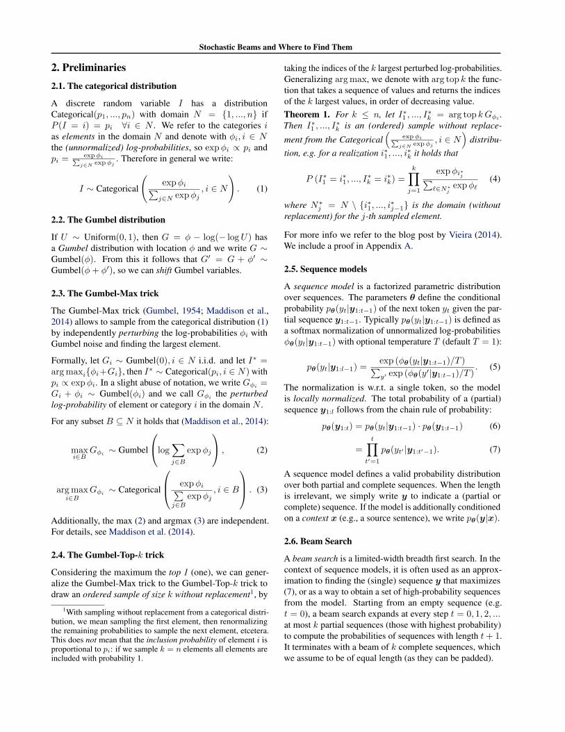
Figure 1. Example of the Gumbel-Top-k trick on a tree, with k = 3. The bars next to the leaves indicate the perturbed log-probabilitiesGφi , while the bars next to internal nodes indicate the maximum perturbed log-probability of the set of leaves S in the subtree rooted atthat node: GφS = maxi∈S Gφi ∼ Gumbel(φS) with φS = log

∑i∈S expφi. The bar is split in two to illustrate that GφS = φS +GS .

Numbers in the nodes represent pθ(yS) = expφS =∑i∈S expφi, the probability of the partial sequence yS . Numbers at edges

represent the conditional probabilities for the next token. The shaded nodes are ancestors of the top k leaves with highest perturbedlog-probability Gφi . These are the ones we actually need to expand. In each layer, there are at most k such nodes, such that we areguaranteed to construct all top k leaves by expanding at least the top k nodes (ranked on GφS ) in each level (indicated by a solid border).

3. Stochastic Beam SearchWe derive Stochastic Beam Search by starting with the ex-plicit application of the Gumbel-Top-k trick to sample k se-quences without replacement from a sequence model. Thisrequires instantiating all sequences in the domain to findthe k largest perturbed log-probabilities. Then we transitionto top-down sampling of the perturbed log-probabilities,and we use Stochastic Beam Search to instantiate (only)the sequences with the k largest perturbed log-probabilities.As both methods are equivalent, Stochastic Beam Searchimplicitly applies the Gumbel-Top-k trick and thus yields asample of k sequences without replacement.

3.1. The Gumbel-Top-k trick on a tree

We represent the sequence model (7) as a tree (as in Figure1), where internal nodes at level t represent partial sequencesy1:t, and leaf nodes represent completed sequences. Weidentify a leaf by its index i ∈ N = {1, ..., n} and writeyi as the corresponding sequence, with (normalized!) log-probability φi = log pθ(y

i). To obtain a sample from thedistribution (7) without replacement, we should sample fromthe set of leaf nodes N without replacement, for which wecan naively use the Gumbel-Top-k trick (Section 2.3):

• Compute φi = log pθ(yi) for all sequences yi, i ∈

N . To reuse computations for partial sequences, thecomplete probability tree is instantiated, as in Figure 1.

• Sample Gφi ∼ Gumbel(φi), so Gφi can be seen as theperturbed log-probability of sequence yi.

• Let i∗1, ..., i∗k = arg top k Gφi , then yi

∗1 , ...,yi

∗k is a

sample of sequences from (7) without replacement.

As instantiating the complete probability tree is computa-tionally prohibitive, we construct an equivalent process thatonly requires computation linear in the number of samplesk and the sequence length.

Perturbed log-probabilities of partial sequences. Forthe naive implementation of the Gumbel-Top-k trick, weonly defined the perturbed log-probabilities Gφi for leafnodes i, which correspond to complete sequences yi. Forthe Stochastic Beam Search implementation, we also de-fine the perturbed log-probabilities for internal nodes corre-sponding to partial sequences. We identify a node (internalor leaf) by the set S of leaves in the corresponding subtree,and we write yS as the corresponding (partial or completed)sequence. Its log-probability φS = log pθ(y

S) can be com-puted incrementally from the parent log-probability using(6), and since the model is locally normalized, it holds that

φS = log pθ(yS) = log

∑i∈S

expφi. (8)

Now for each node S, we define GφS as the maximum of theperturbed log-probabilities Gφi in the subtree leaves S. ByEquation (2), GφS has a Gumbel distribution with locationφS (hence its notation GφS ):

GφS = maxi∈S

Gφi ∼ Gumbel(φS) (9)

Since GφS ∼ Gumbel(φS) is a Gumbel perturbation of thelog-probability φS = log pθ(y

S), we call it the perturbedlog-probability of the partial sequence yS . We can definethe corresponding Gumbel noise GS ∼ Gumbel(0), whichcan be inferred from GφS by the relation GφS = φS +GS .

Stochastic Beams and Where to Find Them

Bottom-up sampling of perturbed log-probabilities.We can recursively compute (9). Write Children(S) as theas the set of direct children of the node S (so Children(S)is a partition of the set S). Since the maximum (9) must beattained in one of the subtrees, it holds that

GφS = maxS′∈Children(S)

GφS′ . (10)

If we want to sample GφS for all nodes, we can use thebottom-up sampling procedure: sample the leaves Gφ{i} =Gφi , i ∈ N and recursively compute GφS using (10). Thisis effectively sampling from the degenerate (constant) distri-bution resulting from conditioning on the children.

Top-down sampling of perturbed log-probabilities.The recursive bottom-up sampling procedure can be inter-preted as ancestral sampling from a tree-structured graph-ical model (somewhat like Figure 1) with edges directedupwards. Alternatively, we can reverse the graphical modeland sample the tree top-down, starting with the root andrecursively sampling the children conditionally.

Note that for the root N (since it contains all leaves N ),it holds that φN = log

∑i∈N expφi = 0, so we can let

GφN ∼ Gumbel(0)2. Starting with S = N , we can re-cursively sample the children conditionally on the parentvariable GφS . For S′ ∈ Children(S) it holds that φS′ =log pθ(y

S′) and we can sample GφS′ ∼ Gumbel(φS′) con-ditionally on (10), e.g. with their maximum equal to GφS .

Sampling a set of Gumbels conditionally on their maxi-mum being equal to a certain value is non-trivial, but canbe done by first sampling the argmax and then samplingthe individual Gumbels conditionally on both the max andargmax. Alternatively, we can let GφS′ ∼ Gumbel(φS′)independently and let Z = maxS′∈Children(S)GφS′ . Then

GφS′ = − log(exp(−GφS )− exp(−Z) + exp(−GφS′ ))

is a set of Gumbels with a maximum equal to GφS . See Ap-pendix B for details and numerically stable implementation.

If we recursively sample the complete tree top-down, thisis equivalent to sampling the complete tree bottom-up, andas a result, for all leaves, it holds that (Gφ{i} =)Gφi ∼Gumbel(φi), independently. The benefit of using top-downsampling is that if we are interested only in obtaining thetop k leaves, we do not need to instantiate the complete tree.

Stochastic Beam Search The key idea of StochasticBeam Search is to apply the Gumbel-Top-k trick for a se-quence model, without instantiating the entire tree, by usingtop-down sampling. With top-down sampling, to find the top

2Or we can simply set (e.g. condition on) GφN = 0. This doesnot affect the result by the independence of max and argmax.

k leaves, at every level in the tree we can suffice with onlyexpanding (instantiating the subtree for) the k nodes withhighest perturbed log-probability GφS . To see this, first as-sume that we instantiated the complete tree using top-downsampling and consider the nodes that are ancestors of at leastone of the top k leaves (the shaded nodes in Figure 1). Atevery level t of the tree, there will be at most k such nodes(as each of the top k leaves has only one ancestor at level t),and these nodes will have higher perturbed log-probabilitiesGφS than the other nodes at level t, which do not containa top k leaf in the subtree. This means that if we discardall but the k nodes with highest log-probabilities GφS , weare guaranteed to include the ancestors of the top k leaves.Formally, the k-th highest log-probability of the nodes atlevel t provides a lower bound required to be among the topk leaves, while GφS is an upper bound for the set of leavesS such that it can be discarded or pruned if it is lower thanthe lower bound, so if GφS is not among the top k.

Thus, when we apply the top-down sampling procedure, ateach level we only need to expand the k nodes with thehighest perturbed log-probabilities GφS to end up with thetop k leaves. By the Gumbel-Top-k trick the result is asample without replacement from the sequence model. Theeffective procedure is a beam search over the (stochastically)perturbed log-probabilities GφS for partial sequences yS ,hence the name Stochastic Beam Search. As we use GφSto select the top k partial sequences, we can also think ofGφS as the stochastic score of the partial sequence yS . Weformalize Stochastic Beam Search in Algorithm 1.

Algorithm 1 StochasticBeamSearch(pθ, k)1: Input: one-step probability distribution pθ , beam/sample size k2: Initialize BEAM empty3: add (yN = ∅, φN = 0, GφN = 0) to BEAM

4: for t = 1, . . . , steps do5: Initialize EXPANSIONS empty6: for (yS , φS , GφS ) ∈ BEAM do7: Z ← −∞8: for S′ ∈ Children(S) do9: φS′ ← φS + log pθ(y

S′ |yS)10: Gφ

S′∼ Gumbel(φS′ )

11: Z ← max(Z,GφS′

)

12: end for13: for S′ ∈ Children(S) do14: Gφ

S′← − log(exp(−GφS )− exp(−Z) + exp(−Gφ

S′))

15: add (yS′, φS′ , GφS′

) to EXPANSIONS

16: end for17: end for18: BEAM ← take top k of EXPANSIONS according to G19: end for20: Return BEAM

3.2. Relation to Beam Search

Stochastic Beam Search should not only be considered as asampling procedure, but also as a principled way to random-ize a beam search. As a naive alternative, one could run anordinary beam search, replacing the top-k operation by sam-

Stochastic Beams and Where to Find Them

pling. In this scenario, at each step t of the beam search wecould sample without replacement from the partial sequenceprobabilities pθ(y1:t) using the Gumbel-Top-k trick.

However, in this naive approach, for a low-probability par-tial sequence to be extended to completion, it does not onlyneed to be initially chosen, but it will need to be re-chosen,independently, again with low probability, at each step ofthe beam search. The result is a much lower probabilityto sample this sequence than assigned by the model. Intu-itively, we should somehow commit to a sampling ‘decision’made at step t. However, a hard commitment to generateexactly one descendant for each of the k partial sequencesat step t would prevent generating any two sequences thatshare an initial partial sequence.

Our Stochastic Beam Search algorithm makes a soft commit-ment to a partial sequence (node in the tree) by propagatingthe Gumbel perturbation of the log-probability consistentlydown the subtree. The partial sequence will then be ex-tended as long as its total perturbed log-probability is amongthe top k, but will fall off the beam if, despite the consistentperturbation, another sequence is more promising.

3.3. Relation to rejection sampling

As an alternative to Stochastic Beam Search, we can drawsamples without replacement by rejecting duplicates fromsamples drawn with replacement. However, if the domainis large and the entropy low (e.g. if there are only a fewvalid translations), then rejection sampling requires manysamples and consequently many (expensive) model evalu-ations. Also, we have to estimate how many samples todraw (in parallel) or draw samples sequentially. StochasticBeam Search executes in a single pass, and requires compu-tation linear in the sample size k and the sequence length,which (except for the beam search overhead) is equal to thecomputational requirement for sampling with replacement.

4. Experiments4.1. Diverse Beam Search

In this experiment we compare Stochastic Beam Search asa principled (stochastic) alternative to Diverse Beam Search(Vijayakumar et al., 2018) in the context of neural machinetranslation to obtain a diverse set of translations for a singlesource sentence x. Following the setup by Vijayakumaret al. (2018) we report both diversity as measured by thefraction of unique n-grams in the k translations as well asmean and maximum BLEU score (Papineni et al., 2002) asan indication of the quality of the sample. The maximumBLEU score corresponds to ‘oracle performance’ reportedby Vijayakumar et al. (2018), but we report the mean as wellsince a single good translation and k−1 completely randomsentences scores high on both maximum BLEU score and

diversity, while being undesirable. A good method shouldincrease diversity without sacrificing mean BLEU score.

We compare four different sentence generations methods:Beam Search (BS), Sampling, Stochastic Beam Search(SBS) (sampling without replacement) and Diverse BeamSearch with G groups (DBS(G)) (Vijayakumar et al., 2018).For Sampling and Stochastic Beam Search, we control thediversity using the softmax temperature T in Equation (5).We use T = 0.1, 0.2, ..., 0.8, where a higher T results inhigher diversity. Heuristically, we also vary T for comput-ing the scores with (deterministic) Beam Search. The diver-sity of Diverse Beam Search is controlled by the diversitystrengths parameter, which we vary between 0.1, 0.2, ..., 0.8.We set the number of groups G equal to the sample size k,which Vijayakumar et al. (2018) reported as the best choice.

We modify the Beam Search in fairseq (Ott et al.,2019) to implement Stochastic Beam Search3, and use thefairseq implementations for Beam Search, Samplingand Diverse Beam Search. For theoretical correctness of theStochastic Beam Search, we disable length-normalization(Wu et al., 2016) and early stopping (and therefore also donot use these parameters for the other methods). We usethe pretrained model from Gehring et al. (2017) and use thewmt14.v2.en-fr.newstest2014 4 test set consistingof 3003 sentences. We run the four methods with samplesizes k = 5, 10, 20 and plot the minimum, mean and maxi-mum BLEU score among the k translations (averaged overthe test set) against the average d = 1

4

∑4n=1 dn of 1, 2, 3

and 4-gram diversity, where n-gram diversity is defined as:

dn =# of unique n-grams in k translationstotal # of n-grams in k translations

.

In Figure 2, we represent the results as curves, indicatingthe trade-off between diversity and BLEU score. The pointsindicate datapoints and the dashed lines indicate the (av-eraged) minimum and maximum BLEU score. For thesame diversity, Stochastic Beam Search achieves highermean/maximum BLEU score. Looking at a certain BLEUscore, we observe that Stochastic Beam Search achieves thesame BLEU score as Diverse Beam Search with a signifi-cantly larger diversity. For low temperatures (< 0.5), themaximum BLEU score of Stochastic Beam Search is com-parable to the deterministic Beam Search, so the increaseddiversity does not sacrifice the best element in the sample.Note that Sampling achieves higher mean BLEU score at thecost of diversity, which may be because good translationsare sampled repeatedly. However, the maximum BLEUscore of both Sampling and Diverse Beam Search is lowerthan with Beam Search and Stochastic Beam Search.

3Our code is available at https://github.com/wouterkool/stochastic-beam-search

4https://s3.amazonaws.com/fairseq-py/data/wmt14.v2.en-fr.newstest2014.tar.bz2

Stochastic Beams and Where to Find Them

(a) k = 5 (b) k = 10 (c) k = 20

Figure 2. Minimum, mean and maximum BLEU score vs. diversity for different sample sizes k. Points indicate different tempera-tures/diversity strengths, from 0.1 (low diversity, left in graph) to 0.8 (high diversity, right in graph).

4.2. BLEU score estimation

In our second experiment, we use sampling without replace-ment to evaluate the expected sentence level BLEU scorefor a translation y given a source sentence x. Although weare often interested in corpus level BLEU score, estimationof sentence level BLEU score is useful, for example whentraining using minibatches to directly optimize BLEU score(Ranzato et al., 2016).

We leave dependence of the BLEU score on the source sen-tence x implicit, and write f(y) = BLEU(y,x). Writingthe domain of y (given x) as y1, ...,yn (e.g. all possibletranslations), we want to estimate the following expectation:

Ey∼pθ(y|x) [f(y)] =n∑i=1

pθ(yi|x)f(yi). (11)

Under a Monte Carlo (MC) sampling with replacementscheme with size k, we write S as the set5 of indices ofsampled sequences {yi, i ∈ S} and estimate (11) using

Ey∼pθ(y|x) [f(y)] ≈1

k

∑i∈S

f(yi). (12)

If the distribution pθ has low entropy (for example if thereare only few valid translations), then MC estimation maybe inefficient since repeated samples are uninformative. Wecan use sampling without replacement as an improvement,but we need to use importance weights to correct for thechanged sampling probabilities. Using the Gumbel-Top-k trick, we can implement an estimator equivalent to theestimator described by Vieira (2017), derived from prioritysampling (Duffield et al., 2007):

Ey∼pθ(y|x) [f(y)] ≈∑i∈S

pθ(yi|x)

qθ,κ(yi|x)f(yi) (13)

Here κ is the (k + 1)-th largest element of {Gφi , i ∈ N},which can be considered the empirical threshold for theGumbel-Top-k trick (since i ∈ S ifGφi > κ), and we define

5Formally, when sampling with replacement, S is a multiset.

qθ,a(yi|x) = P (Gφi > a) = 1 − exp(− exp(φi − a)). If

we would assume a fixed threshold a and variably sized sam-ple S = {i ∈ N : Gφi > a}, then qθ,a(yi|x) = P (i ∈ S)and pθ(y

i|x)qθ,a(yi|x) is a standard importance weight. Surpris-

ingly, using a fixed sample size k (and empirical thresholdκ) also yields in an unbiased estimator, and we include aproof adapted from Duffield et al. (2007) and Vieira (2017)in Appendix D. To obtain κ, we need to sacrifice the lastsample6, slightly increasing variance.

Empirically, the estimator (13) has high variance, and inpractice it is preferred to normalize the importance weightsby W (S) =

∑i∈S

pθ(yi|x)

qθ,κ(yi|x) (Hesterberg, 1988):

Ey∼pθ(y|x) [f(y)] ≈1

W (S)

∑i∈S

pθ(yi|x)

qθ,κ(yi|x)f(yi). (14)

The estimator (14) is biased but consistent: in the limitk = n we sample the entire domain, so we have empiricalthreshold κ = −∞ and qθ,κ(yi|x) = 1 and W (S) = 1,such that (14) is equal to (11).

We have to take care computing the importance weights asdepending on the entropy the terms in the quotient pθ(y

i|x)qθ,κ(yi|x)

can become very small, and in our case the computation ofP (Gφi > a) = 1 − exp(− exp(φi − a)) can suffer fromcatastrophic cancellation. For details, see Appendix C.

Because the model is not trained to use its own predictionsas input, at test time errors can accumulate. As a result,when sampling with the default temperature T = 1, theexpected BLEU score is very low (below 10). To improvequality of generated sentences we use lower temperaturesand experiment with T = 0.05, 0.1, 0.2, 0.5. We then usedifferent methods to estimate the BLEU score:

• Monte Carlo (MC), using Equation (12).

6For Stochastic Beam Search, we use a sample/beam size k, setκ equal to the k-th largest perturbed log-probability and compute(13) based on the remaining k − 1 samples. Alternatively, wecould use a beam size of k + 1.

Stochastic Beams and Where to Find Them

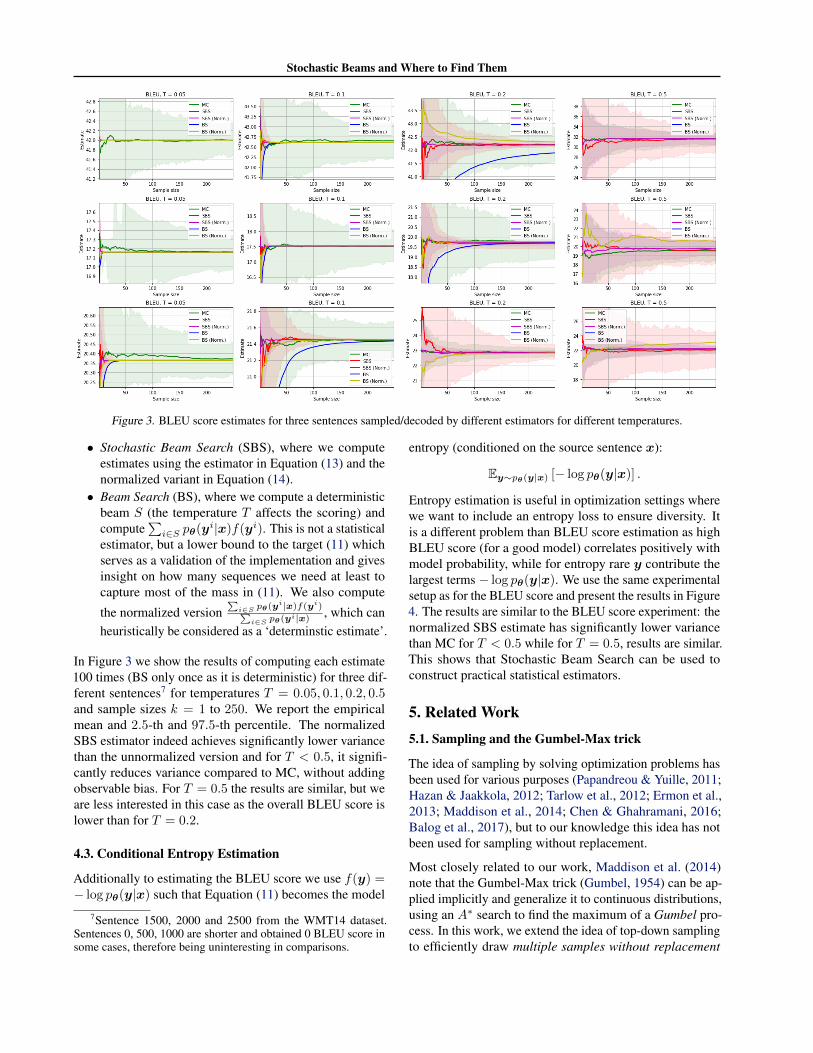
Figure 3. BLEU score estimates for three sentences sampled/decoded by different estimators for different temperatures.

• Stochastic Beam Search (SBS), where we computeestimates using the estimator in Equation (13) and thenormalized variant in Equation (14).

• Beam Search (BS), where we compute a deterministicbeam S (the temperature T affects the scoring) andcompute

∑i∈S pθ(y

i|x)f(yi). This is not a statisticalestimator, but a lower bound to the target (11) whichserves as a validation of the implementation and givesinsight on how many sequences we need at least tocapture most of the mass in (11). We also compute

the normalized version∑i∈S pθ(y

i|x)f(yi)∑i∈S pθ(y

i|x) , which canheuristically be considered as a ‘determinstic estimate’.

In Figure 3 we show the results of computing each estimate100 times (BS only once as it is deterministic) for three dif-ferent sentences7 for temperatures T = 0.05, 0.1, 0.2, 0.5and sample sizes k = 1 to 250. We report the empiricalmean and 2.5-th and 97.5-th percentile. The normalizedSBS estimator indeed achieves significantly lower variancethan the unnormalized version and for T < 0.5, it signifi-cantly reduces variance compared to MC, without addingobservable bias. For T = 0.5 the results are similar, but weare less interested in this case as the overall BLEU score islower than for T = 0.2.

4.3. Conditional Entropy Estimation

Additionally to estimating the BLEU score we use f(y) =− log pθ(y|x) such that Equation (11) becomes the model

7Sentence 1500, 2000 and 2500 from the WMT14 dataset.Sentences 0, 500, 1000 are shorter and obtained 0 BLEU score insome cases, therefore being uninteresting in comparisons.

entropy (conditioned on the source sentence x):

Ey∼pθ(y|x) [− log pθ(y|x)] .

Entropy estimation is useful in optimization settings wherewe want to include an entropy loss to ensure diversity. Itis a different problem than BLEU score estimation as highBLEU score (for a good model) correlates positively withmodel probability, while for entropy rare y contribute thelargest terms − log pθ(y|x). We use the same experimentalsetup as for the BLEU score and present the results in Figure4. The results are similar to the BLEU score experiment: thenormalized SBS estimate has significantly lower variancethan MC for T < 0.5 while for T = 0.5, results are similar.This shows that Stochastic Beam Search can be used toconstruct practical statistical estimators.

5. Related Work5.1. Sampling and the Gumbel-Max trick

The idea of sampling by solving optimization problems hasbeen used for various purposes (Papandreou & Yuille, 2011;Hazan & Jaakkola, 2012; Tarlow et al., 2012; Ermon et al.,2013; Maddison et al., 2014; Chen & Ghahramani, 2016;Balog et al., 2017), but to our knowledge this idea has notbeen used for sampling without replacement.

Most closely related to our work, Maddison et al. (2014)note that the Gumbel-Max trick (Gumbel, 1954) can be ap-plied implicitly and generalize it to continuous distributions,using an A∗ search to find the maximum of a Gumbel pro-cess. In this work, we extend the idea of top-down samplingto efficiently draw multiple samples without replacement

Stochastic Beams and Where to Find Them

Figure 4. Entropy score estimates for three sentences sampled/decoded by different estimators for different temperatures.

from a factorized distribution (with possibly exponentiallylarge domain) by implicitly applying the Gumbel-Top-ktrick. This is a new and practical sampling method.

The blog post by Vieira (2014) describes the relation ofthe Gumbel-Top-k trick (as we call it) to Weighted Reser-voir Sampling (Efraimidis & Spirakis, 2006), an algorithmfor drawing weighted samples without replacement, eitherfrom a stream or efficiently in parallel. When samplingthe complete domain, this is equivalent to the Thurstonian(Thurstone, 1927) interpretation of the Plackett-Luce rank-ing model (Plackett, 1975; Luce, 1959) as given by Yellott(1977). The connection of the Plackett-Luce model to theGumbel-Max trick and the implication that this can be usedfor sampling without replacement is not widely known8.

The Gumbel-Max trick has also been used to define relax-ations of the categorical distribution (Maddison et al., 2016;Jang et al., 2016), which can be reparameterized for low-variance but biased gradient estimators. Recently, Groveret al. (2019) extended this idea to the Plackett-Luce distribu-tion to optimize stochastic sorting networks. We think ourwork is a step in the direction to improve these methods inthe context of sequence models (Gu et al., 2018).

5.2. Beam search

Beam search is widely used for approximate inference invarious domains such as machine translation (Sutskeveret al., 2014; Bahdanau et al., 2015; Ranzato et al., 2016;Vaswani et al., 2017; Gehring et al., 2017), image captioning

8For example, currently the popular PyTorch (Paszke et al.,2017) library uses the (for large k) expensive sequential algorithm.

(Vinyals et al., 2015b), speech recognition (Graves et al.,2013) and other structured prediction settings (Vinyals et al.,2015a; Weiss et al., 2015). Although typically a test-timeprocedure, there are works that include beam search in thetraining loop (Daume et al., 2009; Wiseman & Rush, 2016;Edunov et al., 2018b; Negrinho et al., 2018; Edunov et al.,2018a) for training sequence models on the sequence level(Ranzato et al., 2016; Bahdanau et al., 2017). Many variantsof beam search have been developed, such as a continuousrelaxation (Goyal et al., 2018), diversity encouraging vari-ants (Li et al., 2016; Shao et al., 2017; Vijayakumar et al.,2018) or using modifications such as length-normalization(Wu et al., 2016) or simply applying noise to the output(Edunov et al., 2018a). Our Stochastic Beam Search is aprincipled alternative that shares some of the benefits ofthese heuristic variants, such as the ability to control diver-sity or produce randomized output.

6. DiscussionWe introduced Stochastic Beam Search: an algorithm thatis easy to implement on top of a beam search as a way tosample sequences without replacement. This algorithm re-lates sampling and beam search, combining advantages ofthese two methods. Our experiments support the idea that itcan be used as a drop-in replacement in places where sam-pling or beam search is used. In fact, our experiments showStochastic Beam Search can be used to yield lower-varianceestimators and high-diversity samples from a neural ma-chine translation model. In future work, we plan to leveragethe probabilistic interpretation of beam search to developnew beam search related statistical learning methods.

Stochastic Beams and Where to Find Them

ReferencesBahdanau, D., Cho, K., and Bengio, Y. Neural machine

translation by jointly learning to align and translate. InInternational Conference on Learning Representations,2015.

Bahdanau, D., Brakel, P., Xu, K., Goyal, A., Lowe, R.,Pineau, J., Courville, A., and Bengio, Y. An actor-criticalgorithm for sequence prediction. In International Con-ference on Learning Representations, 2017.

Balog, M., Tripuraneni, N., Ghahramani, Z., and Weller,A. Lost relatives of the gumbel trick. In InternationalConference on Machine Learning (ICML), pp. 371–379.PMLR, 2017.

Chen, Y. and Ghahramani, Z. Scalable discrete sampling as amulti-armed bandit problem. In International Conferenceon Machine Learning, pp. 2492–2501, 2016.

Daume, H., Langford, J., and Marcu, D. Search-basedstructured prediction. Machine learning, 75(3):297–325,2009.

Duffield, N., Lund, C., and Thorup, M. Priority samplingfor estimation of arbitrary subset sums. Journal of theACM (JACM), 54(6):32, 2007.

Edunov, S., Ott, M., Auli, M., and Grangier, D. Understand-ing back-translation at scale. In Proceedings of the 2018Conference on Empirical Methods in Natural LanguageProcessing, pp. 489–500, 2018a.

Edunov, S., Ott, M., Auli, M., Grangier, D., et al. Classi-cal structured prediction losses for sequence to sequencelearning. In Proceedings of the 2018 Conference of theNorth American Chapter of the Association for Com-putational Linguistics: Human Language Technologies,Volume 1 (Long Papers), volume 1, pp. 355–364, 2018b.

Efraimidis, P. S. and Spirakis, P. G. Weighted randomsampling with a reservoir. Information Processing Letters,97(5):181–185, 2006.

Ermon, S., Gomes, C. P., Sabharwal, A., and Selman, B.Embed and project: Discrete sampling with universalhashing. In Advances in Neural Information ProcessingSystems, pp. 2085–2093, 2013.

Gehring, J., Auli, M., Grangier, D., Yarats, D., and Dauphin,Y. N. Convolutional sequence to sequence learning. InInternational Conference on Machine Learning, pp. 1243–1252, 2017.

Goyal, K., Neubig, G., Dyer, C., and Berg-Kirkpatrick, T.A continuous relaxation of beam search for end-to-endtraining of neural sequence models. In Thirty-SecondAAAI Conference on Artificial Intelligence (AAAI), 2018.

Graves, A., Mohamed, A.-r., and Hinton, G. Speech recog-nition with deep recurrent neural networks. In Acoustics,Speech and Signal Processing, IEEE international con-ference on, pp. 6645–6649, 2013.

Grover, A., Wang, E., Zweig, A., and Ermon, S. Stochasticoptimization of sorting networks via continuous relax-ations. In International Conference on Learning Repre-sentations, 2019.

Gu, J., Im, D. J., and Li, V. O. Neural machine translationwith Gumbel-greedy decoding. In Thirty-Second AAAIConference on Artificial Intelligence (AAAI), 2018.

Gumbel, E. J. Statistical theory of extreme values and somepractical applications: a series of lectures. Number 33.US Govt. Print. Office, 1954.

Hazan, T. and Jaakkola, T. On the partition function andrandom maximum a-posteriori perturbations. In Proceed-ings of the 29th International Conference on MachineLearning, pp. 1667–1674. Omnipress, 2012.

Hesterberg, T. C. Advances in importance sampling. PhDthesis, Stanford University, 1988.

Jang, E., Gu, S., and Poole, B. Categorical reparameteriza-tion with gumbel-softmax. In International Conferenceon Learning Representations, 2016.

Li, J., Monroe, W., and Jurafsky, D. A simple, fast diversedecoding algorithm for neural generation. arXiv preprintarXiv:1611.08562, 2016.

Luce, R. D. Individual choice behavior. 1959.

Machler, M. Accurately computing log(1 − exp(−|a|))assessed by the Rmpfr package, 2012. URL https://cran.r-project.org/web/packages/Rmpfr/vignettes/log1mexp-note.pdf.

Maddison, C. J., Tarlow, D., and Minka, T. A* sampling. InAdvances in Neural Information Processing Systems, pp.3086–3094, 2014.

Maddison, C. J., Mnih, A., and Teh, Y. W. The concretedistribution: A continuous relaxation of discrete randomvariables. In International Conference on Learning Rep-resentations, 2016.

Negrinho, R., Gormley, M., and Gordon, G. J. Learningbeam search policies via imitation learning. In Advancesin Neural Information Processing Systems, pp. 10673–10682, 2018.

Ott, M., Edunov, S., Baevski, A., Fan, A., Gross, S., Ng,N., Grangier, D., and Auli, M. fairseq: A fast, extensibletoolkit for sequence modeling. In Proceedings of NAACL-HLT 2019: Demonstrations, 2019.

Stochastic Beams and Where to Find Them

Papandreou, G. and Yuille, A. L. Perturb-and-map randomfields: Using discrete optimization to learn and samplefrom energy models. In Computer Vision (ICCV), IEEEInternational Conference on, pp. 193–200, 2011.

Papineni, K., Roukos, S., Ward, T., and Zhu, W.-J. Bleu:a method for automatic evaluation of machine transla-tion. In Proceedings of the 40th Annual Meeting of theAssociation for Computational Linguistics, pp. 311–318,2002.

Paszke, A., Gross, S., Chintala, S., Chanan, G., Yang, E.,DeVito, Z., Lin, Z., Desmaison, A., Antiga, L., and Lerer,A. Automatic differentiation in PyTorch. In Advances inNeural Information Processing Systems, 2017.

Plackett, R. L. The analysis of permutations. Journal of theRoyal Statistical Society: Series C (Applied Statistics),24(2):193–202, 1975.

Ranzato, M., Chopra, S., Auli, M., and Zaremba, W. Se-quence level training with recurrent neural networks. InInternational Conference on Learning Representations,2016.

Shao, Y., Gouws, S., Britz, D., Goldie, A., Strope, B., andKurzweil, R. Generating high-quality and informativeconversation responses with sequence-to-sequence mod-els. In Proceedings of the 2017 Conference on Empiri-cal Methods in Natural Language Processing, pp. 2210–2219, 2017.

Sutskever, I., Vinyals, O., and Le, Q. V. Sequence to se-quence learning with neural networks. In Advances inneural information processing systems, pp. 3104–3112,2014.

Tarlow, D., Adams, R., and Zemel, R. Randomized optimummodels for structured prediction. In Artificial Intelligenceand Statistics, pp. 1221–1229, 2012.

Thurstone, L. L. A law of comparative judgement. Psycho-logical Review, 34:278–286, 1927.

Vaswani, A., Shazeer, N., Parmar, N., Uszkoreit, J., Jones,L., Gomez, A. N., Kaiser, Ł., and Polosukhin, I. Atten-tion is all you need. In Advances in Neural InformationProcessing Systems, pp. 5998–6008, 2017.

Vieira, T. Gumbel-max trick and weightedreservoir sampling, 2014. URL https://timvieira.github.io/blog/post/2014/08/01/gumbel-max-trick-and-weighted-reservoir-sampling/.

Vieira, T. Estimating means in a finite universe, 2017.URL https://timvieira.github.io/blog/post/2017/07/03/estimating-means-in-a-finite-universe/.

Vijayakumar, A. K., Cogswell, M., Selvaraju, R. R., Sun,Q., Lee, S., Crandall, D. J., and Batra, D. Diverse beamsearch for improved description of complex scenes. InAAAI, 2018.

Vinyals, O., Fortunato, M., and Jaitly, N. Pointer networks.In Advances in Neural Information Processing Systems,pp. 2692–2700, 2015a.

Vinyals, O., Toshev, A., Bengio, S., and Erhan, D. Show andtell: A neural image caption generator. In Proceedingsof the IEEE Conference on Computer vision and PatternRecognition, pp. 3156–3164, 2015b.

Weiss, D., Alberti, C., Collins, M., and Petrov, S. Structuredtraining for neural network transition-based parsing. InProceedings of the 53rd Annual Meeting of the Associa-tion for Computational Linguistics and the 7th Interna-tional Joint Conference on Natural Language Processing(Volume 1: Long Papers), volume 1, pp. 323–333, 2015.

Wiseman, S. and Rush, A. M. Sequence-to-sequence learn-ing as beam-search optimization. In Proceedings of the2016 Conference on Empirical Methods in Natural Lan-guage Processing, pp. 1296–1306, 2016.

Wu, Y., Schuster, M., Chen, Z., Le, Q. V., Norouzi, M.,Macherey, W., Krikun, M., Cao, Y., Gao, Q., Macherey,K., et al. Google’s neural machine translation system:Bridging the gap between human and machine translation.arXiv preprint arXiv:1609.08144, 2016.

Yellott, J. I. The relationship between luce’s choice axiom,thurstone’s theory of comparative judgment, and the dou-ble exponential distribution. Journal of MathematicalPsychology, 15(2):109–144, 1977.

Stochastic Beams and Where to Find Them

A. Proof of the Gumbel-Top-k trickTheorem 1. For k ≤ n, let I∗1 , ..., I

∗k = arg top k Gφi .

Then I∗1 , ..., I∗k is an (ordered) sample without replace-

ment from the Categorical(

expφi∑j∈N expφj

, i ∈ N)

distribu-tion, e.g. for a realization i∗1, ..., i

∗k it holds that

P (I∗1 = i∗1, ..., I∗k = i∗k) =

k∏j=1

expφi∗j∑`∈N∗j

expφ`(15)

where N∗j = N \ {i∗1, ..., i∗j−1} is the domain (withoutreplacement) for the j-th sampled element.

Proof. First note that

P(I∗k = i∗k

∣∣I∗1 = i∗1, ..., I∗k−1 = i∗k−1

)=P

(i∗k = argmax

i∈N∗kGφi

∣∣∣∣∣I∗1 = i∗1, ..., I∗k−1 = i∗k−1

)

=P

(i∗k = argmax

i∈N∗kGφi

∣∣∣∣∣maxi∈N∗k

Gφi < Gφi∗k−1

)(16)

=P

(i∗k = argmax

i∈N∗kGφi

)(17)

=expφi∗k∑`∈N∗k

expφ`. (18)

The step from (16) to (17) follows from the independence ofthe max and argmax (Section 2.3) and the step from (17)to (18) uses the Gumbel-Max trick. The proof follows byinduction on k. The case k = 1 is the Gumbel-Max trick,while if we assume the result (15) proven for k − 1, then

P (I∗1 = i∗1, ..., I∗k = i∗k)

=P(I∗k = i∗k

∣∣I∗1 = i∗1, ..., I∗k−1 = i∗k−1

)· P(I∗1 = i∗1, ..., I

∗k−1 = i∗k−1

)=

expφi∗k∑`∈N∗k

expφ`·k−1∏j=1

expφi∗j∑`∈N∗j

expφ`(19)

=

k∏j=1

expφi∗j∑`∈N∗j

expφ`.

In (19) we have used Equation (18) and Equation (15) fork − 1 by induction.

B. Sampling set of Gumbels with maximum T

B.1. The truncated Gumbel distribution

A random variable G′ has a truncated Gumbel distri-bution with location φ and maximum T (e.g. G′ ∼TruncatedGumbel(φ, T )) with CDF Fφ,T (g) if:

Fφ,T (g)

=P (G′ ≤ g)=P (G ≤ g|G ≤ T )

=P (G ≤ g ∩G ≤ T )

P (G ≤ T )

=P (G ≤ min(g, T ))

P (G ≤ T )

=Fφ(min(g, T ))

Fφ(T )

=exp(− exp(φ−min(g, T )))

exp(− exp(φ− T ))= exp(exp(φ− T )− exp(φ−min(g, T ))). (20)

The inverse CDF is:

F−1φ,T (u) = φ− log(exp(φ− T )− log u). (21)

B.2. Sampling set of Gumbels with maximum T

In order to sample a set of Gumbel variables{Gφi |maxi Gφi = T}, e.g. with their maximum be-ing exactly T , we can first sample the argmax, i∗ and thensample the Gumbels conditionally on both the max andargmax:

1. Sample i∗ ∼ Categorical(

expφi∑j expφj

). We do not

need to condition on T since the argmax i∗ is in-dependent of the max T (Section 2.3).

2. Set Gφi∗ = T , since this follows from conditioning onthe max T and argmax i∗.

3. Sample Gφi ∼ TruncatedGumbel(φi, T ) for i 6= i∗.This works because, conditioning on the max T andargmax i∗, it holds that:

P (Gφi < g|maxiGφi = T, argmax

iGφi = i∗, i 6= i∗)

= P (Gφi < g|Gφi < T ).

Equivalently, we can let Gφi ∼ Gumbel(φi), let Z =maxiGφi and define

Gφi = F−1φi,T(Fφi,Z(Gφi))

= φi − log(exp(φi − T )− exp(φi − Z) + exp(φi −Gφi))

= − log(exp(−T )− exp(−Z) + exp(−Gφi)).(22)

Stochastic Beams and Where to Find Them

Here we have used (20) and (21). Since the transformation(22) is monotonically increasing, it preserves the argmaxand it follows from the Gumbel-Max trick (3) that

argmaxi

Gφi = argmaxi

Gφi ∼ Categorical

(expφi∑j expφj

).

We can think of this as using the Gumbel-Max trick for step1 (sampling the argmax) in the sampling process describedabove. Additionally, for i = argmaxiGφi :

Gφi = F−1φi,T(Fφi,Z(Gφi)) = F−1φi,T

(Fφi,Z(Z)) = T

so here we recover step 2 (setting Gφi∗ = T ). For i 6=argmaxiGφi it holds that:

P (Gφi ≤ g|i 6= argmaxi

Gφi)

=EZ(P (Gφi ≤ g|Z, i 6= argmaxi

Gφi))

=EZ(P (Gφi ≤ g|Z,Gφi < Z))

=EZ(P (F−1φi,T(Fφi,Z(Gφi)) ≤ g|Z,Gφi < Z))

=EZ(P (Gφi ≤ F−1φi,Z(Fφi,T (g))|Z,Gφi < Z))

=EZ(Fφi,Z(F−1φi,Z

(Fφi,T (g))))

=EZ(Fφi,T (g)) = Fφi,T (g).

This means that Gφi ∼ TruncatedGumbel(φi, T ),so this is equivalent to step 3 (sampling Gφi ∼TruncatedGumbel(φi, T ) for i 6= i∗).

B.3. Numeric stability of truncated Gumbelcomputation

Direct computation of (22) can be unstable as large termsneed to be exponentiated. Instead, we compute:

vi = T −Gφi + log1mexp(Gφi − Z) (23)

Gφi = T −max(0, vi)− log1pexp(−|vi|) (24)

where we have defined

log1mexp(a) = log(1− exp(a)), a ≤ 0

log1pexp(a) = log(1 + exp(a)).

This is equivalent as

T −max(0, vi)− log(1 + exp(−|vi|))=T − log(1 + exp(vi))

=T − log (1 + exp (T −Gφi + log (1− exp (Gφi − Z))))=T − log (1 + exp (T −Gφi) (1− exp (Gφi − Z)))=T − log (1 + exp (T −Gφi)− exp (T − Z))= − log (exp(−T ) + exp(−Gφi)− exp(−Z))= Gφi

The first step can be easily verified by considering thecases vi < 0 and vi ≥ 0. log1mexp and log1pexp canbe computed accurately using log1p(a) = log(1 + a) andexpm1(a) = exp(a)− 1 (Machler, 2012):

log1mexp(a) =

{log(− expm1(a)) a > −0.693log1p(− exp(a)) otherwise

log1pexp(a) =

{log1p(exp(a)) a < 18

x+ exp(a) otherwise

C. Numerical stability of importance weightsWe have to take care computing the importance weightsas depending on the entropy the terms in the quotientpθ(yi|x)qθ(yi|x) can become very small, and in our case the com-putation of P (Gφi > κ) = 1 − exp(− exp(φi − κ))can suffer from catastrophic cancellation. We can rewritethis expression using the more numerically stable imple-mentation exp1m(x) = exp(x) − 1 as p(Gφi > κ) =−exp1m(− exp(φi− κ)) but in some cases this still suffersfrom instability as exp(φi − κ) can underflow if φi − κ issmall. Instead, for φi − κ < −10 we use the identity

log(1− exp(−z)) = log(z)− z

2+z2

24− z4

2880+O(z6)

to directly compute the log importance weight using z =exp(φi − κ) and φi = log pθ(yi|x) (we assume φi is nor-malized):

log

(pθ(yi|x)qθ(yi|x)

)= log pθ(yi|x)− log qθ(yi|x)

= log pθ(yi|x)− log (1− exp(− exp(φi − κ)))= log pθ(yi|x)− log (1− exp(−z))

= log pθ(yi|x)−(log(z)− z

2+z2

24− z4

2880+O(z6)

)= log pθ(yi|x)−

(φi − κ−

z

2+z2

24− z4

2880+O(z6)

)=κ+

z

2− z2

24+

z4

2880+O(z6)

If φi − κ < −10 then 0 < z < 10−6 so this computationwill not lose any significant digits.

Stochastic Beams and Where to Find Them

D. Proof of unbiasedness of priority samplingestimator

The following proof is adapted from the proofs by Duffieldet al. (2007) and Vieira (2017). For generality of the proof,we write f(i) = f(yi), pi = pθ(y

i|x) and qi(κ) =qθ,κ(y

i|x), and we consider general keys hi (not neces-sarily Gumbel perturbations).

We assume we have a probability distribution over a fi-nite domain 1, ..., n with normalized probabilities pi, e.g.∑ni=1 pi = 1. For a given function f(i) we want to estimate

the expectation

E[f(i)] =n∑i=1

pif(i).

Each element i has an associated random key hi and wedefine qi(a) = P (hi > a). This way, if we know thethreshold a it holds that qi(a) = P (i ∈ S) is the probabilitythat element i is in the sample S. As was noted by Vieira(2017), the actual distribution of the key does not influencethe unbiasedness of the estimator but does determine theeffective sampling scheme. Using the Gumbel perturbedlog-probabilities as keys (e.g. hi = Gφi) is equivalent tothe PPSWOR scheme described by Vieira (2017).

We define shorthand notation h1:n = {h1, ..., hn}, h−i ={h1, ..., hi−1, hi+1, ..., hn} = h1:n \ {hi}. For a givensample size k, let κ be the (k+1)-th largest element of h1:n,so κ is the empirical threshold. Let κ′i be the k-th largestelement of h−i (the k-th largest of all other elements).

Similar to Duffield et al. (2007) we will show that everyelement i in our sample contributes an unbiased estimateof E[f(i)], so that the total estimator is unbiased. Formally,we will prove that

Eh1:n

[1{i∈S}

qi(κ)

]= 1 (25)

from which the result follows:

Eh1:n

[∑i∈S

piqi(κ)

f(i)

]

=Eh1:n

[n∑i=1

piqi(κ)

f(i)1{i∈S}

]

=

n∑i=1

pif(i) · Eh1:n

[1{i∈S}

qi(κ)

]

=

n∑i=1

pif(i) · 1 =

n∑i=1

pif(i) = E[f(i)]

To prove (25), we make use of the observation (slightlyrephrased) by Duffield et al. (2007) that conditioning on

h−i, we know κ′i and the event i ∈ S implies that κ = κ′isince i will only be in the sample if hi > κ′i which meansthat κ′i is the k + 1-th largest value of h−i ∪ {hi} = h1:n.The reverse is also true (if κ = κ′i then hi must be largerthan κ′i since otherwise the k + 1-th largest value of h1:nwill be smaller than κ′i).

Eh1:n

[1{i∈S}

qi(κ)

]=Eh−i

[Ehi

[1{i∈S}

qi(κ)

∣∣∣∣hi]]=Eh−i

[Ehi

[1{i∈S}

qi(κ)

∣∣∣∣h−i, i ∈ S]P (i ∈ S|h−i)+Ehi

[1{i∈S}

qi(κ)

∣∣∣∣h−i, i 6∈ S]P (i 6∈ S|h−i)]=Eh−i

[Ehi

[1

qi(κ)

∣∣∣∣h−i, i ∈ S]P (i ∈ S|h−i) + 0

]=Eh−i

[Ehi

[1

qi(κ)

∣∣∣∣h−i, i ∈ S] qi(κ′i)]=Eh−i

[Ehi

[1

qi(κ)

∣∣∣∣κ = κ′i

]qi(κ

′i)

]=Eh−i

[Ehi

[1

qi(κ′i)

]qi(κ

′i)

]=Eh−i

[1

qi(κ′i)qi(κ

′i)

]= Eh−i [1] = 1