step solar thermal - utah
TRANSCRIPT

STEP Solar Thermal
Aaron T. Bame
Joseph Furner
Brian D. Iverson
March 5, 2021
1

AcronymsBFP Boiler Feed Pump
BFPT Boiler Feed Pump Turbine
CC Capital Cost
CO2 Carbon Dioxide
CP Condensate Pump
CSDNI Clear Sky Direct Normal Insolation [W m-2]
CSP Concentrating Solar Power
DA Deaerator
DC Drain Cooler
DNI Direct Normal Insolation [W m-2]
EPRI Electric Power Research Institute
FE Fuel Earnings [USD]
FS Fuel Saving
FWH Feedwater Heater
GHG Greenhouse Gas
HP High Pressure
HPT High Pressure Turbine
HTF Heat Transfer Fluid
IPT Intermediate Pressure Turbine
ISCC Integrated Solar Combined Cycle
LCOE Levelized Cost of Electricity [USD kWh-1]
LFR Linear Fresnel Reflector
LP Low Pressure
LPT Low Pressure Turbine
NG Natural Gas
NREL National Renewable Energy Laboratory
NSRDB National Solar Resource Database
O&M Operation & Maintenance
OBJ Objective
PB Power Boost
PBT Payback Time [years]
PTC Parabolic Trough Collector
PV Photovoltaic
2

PVT Photovoltaic-Thermal
SAM System Advisor Model
SCA Solar Collection Assembly
SI Solar Integration
SX Solar Exchange
TES Thermal Energy Storage
VariablesQB Boiler Heating Power [MW]
Qfo Thermal Equivalent of Fuel Offset [MW]
W Mechanical Power [MW]
η Efficiency [%]
ηc CSP Collection Efficiency [%]
ηsu Solar Use Efficiency [%]
ηth Thermal Efficiency [%]
ηII 2nd Law Efficiency [%]
ω Optimization Objective Weight [-]
A Area [m2]
C Cost [USD]
cp,s Specific Heat of Solar Heat Transfer Fluid [kJ kg-1 K-1]
dr Receiver Diameter [m]
E Total Energy [kWh]
F Conversion Factor
f Optimization Objective [kW-1]
h Specific Enthalpy [kJ kg-1]
hsun Useful Solar Time [hours day-1]
k Augment Fraction [%]
L Length [m]
m Mass Flow Rate [kg s-1]
mef Mass Extraction Fraction [ ]
Nl Number of Solar Field Loops
Na Number of Solar Collection Assemblies per Loop
Ps1 HPT 1st Stage Pressure [MPa]
r Rate or Ratio
3

s Specific Entropy [kJ kg-1 K-1]
T Temperature [K]
T0 Dead State Temperature [K]
Wp Aperture Width [m]
X Exergy Rate [kW]
Subscripts[ ]c Concentration Property
[ ]d Discount Property
[ ]n Annual Value
[ ]p Aperture Property
[ ]r Solar Receiver Property
[ ]s Solar Field/Solar Contribution
[ ]net Net Property
[ ]opt Optimum Property
Financial Variables (Appendix D)A Cumulative Cash Flow
FCR Fixed Charge Rate
DC Direct Costs
Cexp Operation and Maintenance Expenses
CFOM Fixed Operation and Maintenance Costs
Cins Insurance Costs
CP&I Principle and Interest Payment
Ct,prp Property Tax Costs
CVOM Variable Operation and Maintenance Costs
CFF Construction Factor
CRF Capital Recover Factor
EPC Engineering-Procurement-Construction
FL Debt Fraction
FS Fuel Savings
IC Indirect Costs
IRR Internal Rate of Return
ITC Investment Tax Credit
4

Lnet,0 Initial Loan Balance
NL Loan Period
PFF Project Factor
PTC Project Tax Credit
rd Discount Rate
ri Inflation Rate
rint Loan Interest Rate
S Savings
SCdep Depreciation Schedule
WACC Weighted Average of Component Costs
[ ]an Annual
[ ]con Construction
[ ]cont Contingency
[ ]Fed Federal
[ ]nom Nominal
[ ]r Real
[ ]sal Sales
[ ]SI Site Improvements
[ ]st State
[ ]t Tax
5
Executive Summary
The objectives of this study were outlined in a statement of work at the commencement of the
study. This study was meant to address the viability of integrating concentrated solar power with
coal-fired power plants including the Hunter Unit 3 in Castle Dale, UT. To be of use in future
evaluations, this study was intended to identify a general plant model that could be used to deter-
mine hybrid feasibility and the optimization of solar integration into a general hybrid plant model.
This report describes in depth the development of computational models used to evaluate hybrid
feasibility, results for Hunter Unit 3 hybrid feasibility, and possible results for other coal plants un-
der different conditions. Of particular interest was the impact of hybridization on the coal plant’s
thermodynamics, the financial impact (capital cost, levelized cost of electricity, and payback time),
and the application of these methods to other power plants for future evaluations.
To extend the application of this study, a representative power plant model was designed to
approximate coal power plant performance for plants of differing configurations. The primary
simplification in the representative plant model is the reduction of feedwater heaters. Several feed-
water heaters are placed in series to incrementally preheat the water of a coal power plant prior to
the primary heating done in the boiler. However, each coal power plant has different configura-
tions of feedwater heaters at high and low pressures. The representative model approximates the
feedwater heating process using a single feedwater heater at each of the low and high pressures.
Section 2.1 describes the process of evaluating feedwater heater operating properties, the impli-
cations of combining feedwater heaters, other simplifications made to achieve the representative
model used throughout the study, and validation of the representative model with data published in
archival literature.
A model for estimating the solar resource for Castle Dale, UT was developed and general-
ized to be applicable to any location, provided there is meteorological data available through the
National Renewable Energy Laboratory. This solar resource model approximates the multi-year
average direct normal insolation which is used to estimate the amount of solar equipment required
to achieve any given solar augment fraction. Section 2.2 describes in detail the method of cal-
culating the multi-year average direct normal insolation, the method of estimating the size of the
solar field, and descriptions of the solar collection hardware and heat transfer fluids assumed as
benchmark products.
The integration of the solar resource in the overall hybrid plant model and the interactions with
the surrounding coal power plant are described in Sections 2.3 and 2.4. The possible options for
solar integration are discussed along with the introduction of the solar work contribution, defined
here as the amount of power generated by the hybrid plant that can be attributed to the integration
6

of the solar resource.
While solar hybridization is shown to have thermodynamic benefits to fossil-fueled power
plants, the financial impact is an important factor when considering real applications as opposed to
theoretical implementation. The financial model description is included in Section 2.5. The finan-
cial calculations are based on the financial model used as part of the National Renewable Energy
Laboratory’s System Advisor Model and modified to be applicable to hybrid plants. Section 2.5
describes how the savings from fuel offset due to solar integration are used to calculate the payback
time for the solar field and the marginal solar levelized cost of electricity.
The solar integration model and financial model are used to calculate the parameters used in
the objective function for the optimization of solar hybridization: solar contribution, fuel offset,
levelized cost of electricity, payback time 1, and total fuel earnings. The optimization is constrained
by the requirements that the payback time 1 must be less than the expected life of the hybrid plant
and that the solar field fit within the maximum land use available. More details on the calculation
of the optimization objective and the searching algorithm are provided in Section 2.6.
The results for Hunter Unit 3 are that concentrated solar power hybridization is not feasible at
this time. Because complete feedwater heater bypass was chosen as the solar integration method,
a minimum augment fraction of 3% is required to offset coal use and see any financial benefit.
However, the land area identified by the Hunter plant as an available candidate for a solar field is
insufficient to accommodate augment fractions greater than 3%. Hybridization with Hunter Unit 3
is also infeasible financially. Payback times for integration with the Hunter Unit exceed expected
project life for all configurations.
Though hybridization has been shown to be infeasible for the Hunter Unit 3 power plant, hy-
bridization is still beneficial for other situations. Green energy premium prices and carbon taxes
are common local incentives that improve financial feasibility for hybridization projects. Califor-
nia has a price of carbon in place at 16 USD sh.tn.-1. A green premium price of 0.018 USD kWh-1
has been reported as an average price common to US markets. Both the carbon price and the green
premium are shown in this report to increase the feasibility of hybridization. In areas with either
a carbon tax, green premium price, or both, this model can still be used to evaluate preliminary
feasibility. With a 16 USD sh.tn.-1 and no green premium, the optimal configuration is to bypass
feedwater heater 6 with an augment fraction of 9% solar augmentation provided by a parabolic
trough collector field with a levelized cost of electricity of 9.5××× 10−4 USD kWh-1 and payback
time of 25.2 years. For the same configuration and no carbon tax, the payback time decreases from
62.1 years with no green energy premium to 22.5 years with a green energy premium based on
solar contribution and 3.9 years with a premium based on overall plant output.
7

1 Introduction
1.1 Fossil Fuel vs. Renewable Energy
Fossil fuels have proven to be reliable sources of power for a developing world, accounting for 10-
12% of the energy provided in the US every year since 2010 [1]. Energy consumption in developing
countries has been projected to increase at a rate of 3% per year [2]. As the number of people in
need of electricity continues to climb, the availability of resources capable of power generation
becomes a paramount concern. Additionally, the effect of CO2 and other greenhouse gas (GHG)
emissions from power plants on the environment and global health needs to be addressed. These
concerns lead to regulations that loom over fossil fuel power plants forcing innovation in cleaning
emissions and improving efficiency.
Concerns with fossil fuels have sparked an ongoing debate, the result of which has been the
dramatic increase in power generation using renewable resources such as wind and solar, with
increases from 2018-2019 of 140 and 100 Trillion BTU, respectively [1]. At first glance, renewable
plants seem to solve all the problems associated with fossil fuels in that the resources are naturally
occurring, renewable, and the process for the conversion of the energy to useful power does not
provide harmful emissions.
However, renewable plants are not without drawbacks. The ability to harness a resource is
completely dependent on location. Additionally, renewable power plants tend to have very high
capital costs including transmission, land allocation, and thermal energy storage (TES) that is
often used to meet grid demands when the resource is unavailable or production is inefficient. High
capital costs and low efficiency power generation increase the levelized cost of electricity, or LCOE
(measured in USD/kWh). Capital costs for natural gas combined cycles are approximately 1,000
USD kW-1 compared to 2,000 USD kW-1 for on shore wind and 2,600 USD kW-1 for photovoltaic
systems [3]. Conversion efficiencies for combined cycles can approach 60% while wind turbines
range from 30-40% efficient and photovoltaic panels are typically 10-25% efficient¿ [4]. Effective
locations for resources such as wind and solar are in places that are not densely populated, thus
requiring power transmission. Solar plants do not have a high yield because the conversion process
is simply not efficient enough. Therefore, large plots of land must be allocated for one plant to
support a community. In the US, coal power plants occupy 12.21 ac MW-1 compared to solar
(43.5 ac MW-1) and wind (70.64 ac MW-1) [5]. In conjunction with the large scales that typically
accompany renewable power plants, the cost of development is driven even higher by the wide
use of relatively experimental technology. Perhaps the biggest drawback to renewable plants is
intermittency. Power generation from wind peaks in the evening when there are large thermal
8

gradients through canyons, but power consumption is typically lowest in the evenings. Solar power
is only effective when the sun is visible which presents problems during cloud cover or in the
evening. These high costs and intermittency can preclude the penetration of renewable energy
systems into many markets [6, 7].
One solution proposed in 1975 [8] and further explored in 1993 [9] is to break out of the fossil-
renewable dichotomy and implement hybrid power plants. The source energy for hybrid power
plants may be either predominantly fossil-fuel with renewable augmentation or predominantly re-
newable with fossil-fuel augmentation. A baseload plant is one that continuously supplies at least
the minimum amount of power required throughout the year. The integration of renewable and
fossil fuel sources is able to maintain the necessary energy supply when the renewable resource
availability drops and reduce the amount of carbon-based fuel used with its associated emissions.
Concentrating solar power (CSP) and wind power are the best options for hybridization because
both resources are more universally prevalent than other sources such as geothermal or tidal power.
While wind power plants are limited by the average speed of the local wind, solar radiation can be
used anywhere in the world with varying degrees of efficiency making CSP the most popular can-
didate for hybridization. Since 1993, hybridization has gained substantial international attention
and is often discussed in current literature.
1.2 Evaluating CSP Hybridization Potential
Turchi et al. at National Renewable Energy Laboratory (NREL) have developed a method to eval-
uate hybridization potential for fossil fueled power plants [10]. The method compiles weighted
parameters including plant age, capacity factor, annual average direct normal irradiation (DNI),
available land and slope of the land, and the expected solar use efficiency. The plants are then
rated as Excellent, Good, Fair, or Not Considered based on comparative scores.
The most important category by weight in the NREL study was DNI (35%). Of the 22 states
evaluated in the study, Texas, Arizona, and Florida have the most total hybridization potential,
but only Arizona, Nevada, California, and New Mexico have plants that qualify as Excellent.
According to the National Solar Radiation Database at NREL.gov, the latter 4 states also record
the highest average annual DNI, improving the hybridization score.
After DNI, normal operating plant capacity factor is the next important category (20%). The
solar integration discussed in this and an NREL study is most effective for baseload plants (capacity
factor > 50%) because capital costs can only be repaid as more power is generated. Baseload
plants are operating more and will thus repay the capital comparatively faster than intermediate or
peaking plants (capacity factor < 50%).
9

The land to be used for the collectors (15%) is of interest because the area available can severely
limit the collector area or technology selection depending on the desired solar thermal input. Ad-
ditionally, land with too steep of a grade can inhibit the collector from effectively tracking the
sun.
Finally, solar use efficiency (10%), and age of the plant (5%) are weighted as the least important
parameters. Solar use efficiency is the ratio of power generated by solar contribution to the amount
of energy absorbed by the collectors (ηsu =MWe/MWth). A low weight for solar use efficiency
seems counter-intuitive, but is in place to avoid penalizing plants with large solar collection area
that typically result in lower solar use efficiency. The main purpose in hybridization is to reduce
fossil fuel consumption and overall GHG emissions, so while increasing solar collector area can
have a negative impact on solar use efficiency, it has an overall positive impact on the pursuit of
increasing renewable power generation.
1.3 Hybridization capabilities
The NREL study only focused on power plants that used fossil fuels, but CSP can be used to
augment any power generation method. Pramanik and Ravikrishna reviewed the CSP technologies
available for hybridization with fossil fuel plants as well as with biomass, geothermal, and wind
power plants and assigned each combination to a hybrid ranking from low to high. High solar
hybrids used CSP to supplement fuel from biomass, geothermal, and other plants that are already
considered renewable. Medium solar hybrids combine CSP and natural gas as only a supplemental
fuel limited to 15-25% to meet spikes in consumption. Low solar hybrids, the focus of this current
study, use up to 20% CSP to supplement typically coal or natural gas fired Brayton cycles [11] .
There are several medium solar hybrid systems in operation today. The Solar Electric Gener-
ating Systems in California are a collection of nine parabolic trough CSP plants, eight of which
use natural gas as a backup resource. This backup fuel is used to offset volume required for the
TES otherwise necessary in medium hybrid systems. Medium systems leave the designer with a
choice between low LCOE and low GHG emissions. Increasing the amount of solar collector area
will decrease GHG emissions and the amount of fossil fuel required to meet market demands but
increase LCOE. Limiting collecting area will require more fossil fuel supplementation which de-
creases LCOE but increases GHG emissions. Fossil fuels consist of 15-25% of the source energy
consumed in medium systems though individual analysis and optimization must be performed for
each plant and geographic location.
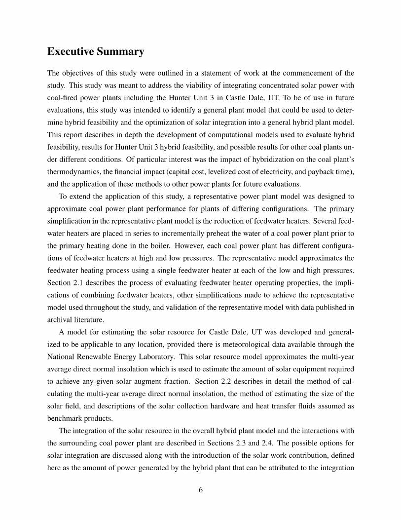
Low solar hybrid systems consist of solar-Brayton cycles, integrated solar combined cycles
(ISCC), and solar-aided coal cycles. Solar-Brayton cycles use the solar thermal technology to
10

(a) (b)
Figure 1: Line focusing technology: a) Parabolic Trough Collector and b) Linear Fresnel Reflec-tor [14].
preheat or superheat the working fluid of the power cycle. Fossil fuels are still burned, but the pre-
heating or superheating increases power output and thermal efficiency. ISCC use heat exchangers
to transfer the solar thermal energy to the working fluid. Solar-aided coal cycles without regenera-
tion often use solar thermal energy to heat the working fluid in place of the steam that is bled off in
standard plants. The results for integration in combined cycles and coal plants are similar to solar-
Brayton, but further analysis is required to evaluate top cycle versus bottom cycle integration for
ISCC. Care must also be given when designing the solar collection area for solar-aided coal plants
if the solar thermal energy is used for feedwater heating because there exists an optimal collection
area such that more collection area does not contribute any more to the coal cycle. Using CSP to
augment coal power plants is of interest because of the higher amount of GHG emissions per unit
energy, compared with natural gas [12].
1.4 CSP Technology
There are three technologies commonly used for solar thermal applications: Parabolic Trough
Collector (PTC), Solar Tower, and Linear Fresnel Reflector (LFR). PTC have been in production
for at least 100 years since Frank Shuman used them to heat steam to power an irrigation pump
in Egypt in 1916 [13]. Since then, PTC have benefited from extensive research that has improved
performance and reduced cost to the point that PTC now owns 94% of the CSP market share.
PTC operate based on geometric properties of parabolas. Any normal radiation will reflect off the
parabolic mirrors and concentrate on the collector tube running along the geometric focus. The
power concentrated on the collector will heat the solar heat transfer fluid (HTF) that will be sent to
integrate with the fossil-fueled power plant.
Solar Tower and LFR have not undergone as much development as PTC but are still viable
options for CSP as stand-alone plants as well as in hybrid plants. Solar towers use a circular
11
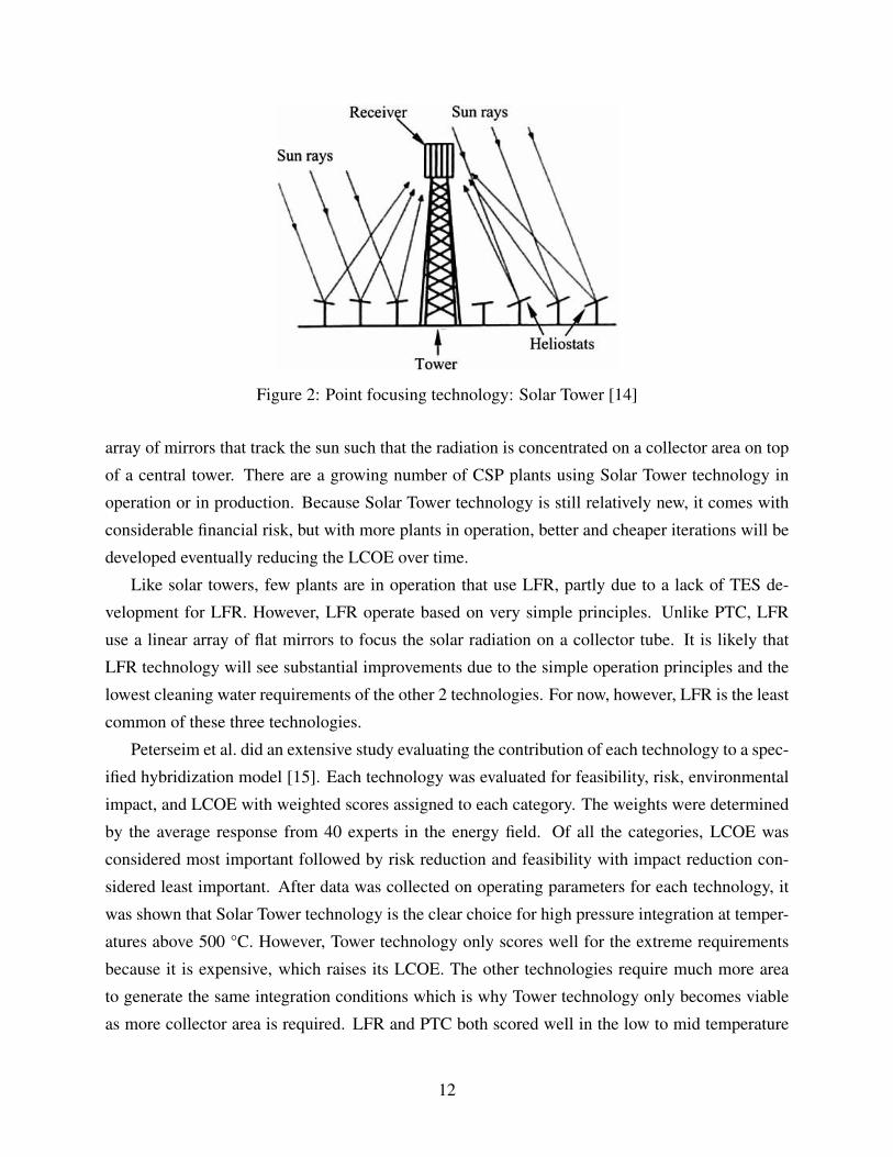
Figure 2: Point focusing technology: Solar Tower [14]
array of mirrors that track the sun such that the radiation is concentrated on a collector area on top
of a central tower. There are a growing number of CSP plants using Solar Tower technology in
operation or in production. Because Solar Tower technology is still relatively new, it comes with
considerable financial risk, but with more plants in operation, better and cheaper iterations will be
developed eventually reducing the LCOE over time.
Like solar towers, few plants are in operation that use LFR, partly due to a lack of TES de-
velopment for LFR. However, LFR operate based on very simple principles. Unlike PTC, LFR
use a linear array of flat mirrors to focus the solar radiation on a collector tube. It is likely that
LFR technology will see substantial improvements due to the simple operation principles and the
lowest cleaning water requirements of the other 2 technologies. For now, however, LFR is the least
common of these three technologies.
Peterseim et al. did an extensive study evaluating the contribution of each technology to a spec-
ified hybridization model [15]. Each technology was evaluated for feasibility, risk, environmental
impact, and LCOE with weighted scores assigned to each category. The weights were determined
by the average response from 40 experts in the energy field. Of all the categories, LCOE was
considered most important followed by risk reduction and feasibility with impact reduction con-
sidered least important. After data was collected on operating parameters for each technology, it
was shown that Solar Tower technology is the clear choice for high pressure integration at temper-
atures above 500 °C. However, Tower technology only scores well for the extreme requirements
because it is expensive, which raises its LCOE. The other technologies require much more area
to generate the same integration conditions which is why Tower technology only becomes viable
as more collector area is required. LFR and PTC both scored well in the low to mid temperature
12
ranges (about 380 °C - 450 °C). PTC scores well due to maturity and LFR scores well due to
efficient land use and comparatively low cleaning water consumption.
1.5 CSP Integration Options
The Electric Power Research Institute (EPRI) conducted a study on different integration locations
for coal and natural gas hybrid plants and ranked the suggested integration points by solar use
efficiency [16]. The integration points for NGCC and coal are listed in the EPRI report. Because
this study is focused on coal hybrid plants, only the integration points suggested for coal plants
will be considered. For their model, it was determined that high-pressure (HP) superheated steam
(about 540 °C) would be the best state to integrate into a coal plant at the main steam header
(ηsu =43-46%), followed by HP slightly superheated steam (about 370 °C) and HP saturated steam
(about 350 °C) both integrated at the HP primary superheater inlet (ηsu =30-42% and 28-40%,
respectively), and finally intermediate-pressure (IP) superheated steam (about 370 °C) for cold
reheating (ηsu =25-28%). Because a different technology would probably be ideal for each of the
integration points above, a method of optimizing the integration point and technology is required,
and should also include an analysis of a hybrid plant expected life cycle.
CSP augmentation of coal power plants offers multiple benefits including a reduction of CO2
with some of the energy resource coming from a renewable source, a reduction in the overall cost
as compared to a stand-alone CSP plant of the same combined capacity, and an increase in avail-
ability and capacity relative to a stand-alone CSP plant [17]. CSP integration also results in higher
solar-to-electric efficiency, reduced costs for retrofitted projects, higher capacity factors without
thermal energy storage, and improved ramping time [18, 19]. Among the various possible appli-
cations of CSP hybridization [20], coal is a popular candidate because CSP and coal share many
of the same power generation components and because of the large presence of coal throughout
the world. However, the possibility of hybridization is affected by more than just thermodynamic
performance [21].
1.6 Benefits of CSP-Hybridization
Zhai et al. studied the life cycle of nine power plant combinations for baseload coal, CSP hybrid,
and CSP hybrid with TES at 300, 600, and 1000 MW outputs [22]. Zhai et al. separated the life
cycle of a CSP hybrid power plant into four phases: Fuel, Operation, Transport, and Materials. The
Fuel phase is defined as the process of converting resources into useful fuel. The Operation stage
is the actual burning of the fuel. The Transportation phase considers hardware transportation and
13
solar thermal HTF transmission. The Materials stage entails the exploitation and transportation of
raw materials.
Each configuration was evaluated from plant construction to the end of the expected life on
a weighted sum of objective scores: (1) global warming potential, (2) acidification potential, (3)
respiratory effects potential, (4) primary energy consumption, and (5) capital costs. Zhai et al.
showed that for each objective value, every hybrid plant performs better than a coal-fired plant
with one exception, capital costs. Pure coal plants became economically comparable to hybrid
configurations as the weight of capital costs increased and surpassed hybrids with a further increase
in the capital weight factor. This means that, when considering hybridization potential, as capital
costs become more important and other economic factors such as carbon tax are neglected, hybrid
viability decreases. Zhai et al. also shows that GHG emissions, including CO2 and SO2, are highest
during the Fuel and Operation stages of a plant life. The integration of CSP reduces the fuel
required to produce the same amount of power and provides significant environmental benefit to
CSP hybrid power plants operating in FS mode such as in Zhai et al.
Manente studied the benefits of hybridization and demonstrated which plant modifications and
operating mode would provide an increase of 50 MWe turbine output power [23]. The plant ana-
lyzed was an integrated solar combined cycle which augments the heating for a natural gas com-
bined cycle. Manente classified the operating modes as power boost (PB) and fuel saving (FS). In
PB mode, solar augmentation is used to increase the power generation holding fuel consumption
constant. The categories of power boost included: no change in plant equipment (PB1); upgrading
steam turbines (PB2) to account for significant increases in turbine output; and upgrading both
turbines and heat exchangers (PB3) to support the increased heat transfer from the solar collectors
and loads on the turbine. In FS mode, solar augmentation is used to hold power generation con-
stant and decrease fuel consumption. FS mode configurations were evaluated for configurations
that required no equipment changes (FS1) and for the case of an upgraded turbine (FS2). The
highest power output increase from solar augmentation was from PB3, but overall plant efficiency
was highest for PB1. PB1 also required less solar collection area (SCA) and was comparable to
PB2 and PB3 in both radiation and thermal-to-electric efficiencies. FS1 required slightly more
augmentation than PB1, but provided a greater power boost and higher solar radiation-to-thermal
efficiency. The hybrid power plants evaluated in this study will be assumed to operate in FS mode,
or net power output will remain constant and the amount of fuel consumption will vary.
Both Behar et al. [24] and Libby [16] suggest that, among other options, solar can be integrated
at a feedwater heater (FWH) where steam, extracted from a turbine, is typically used to preheat
some other working fluid. Downstream effects can be mitigated by selecting the augment fraction
14
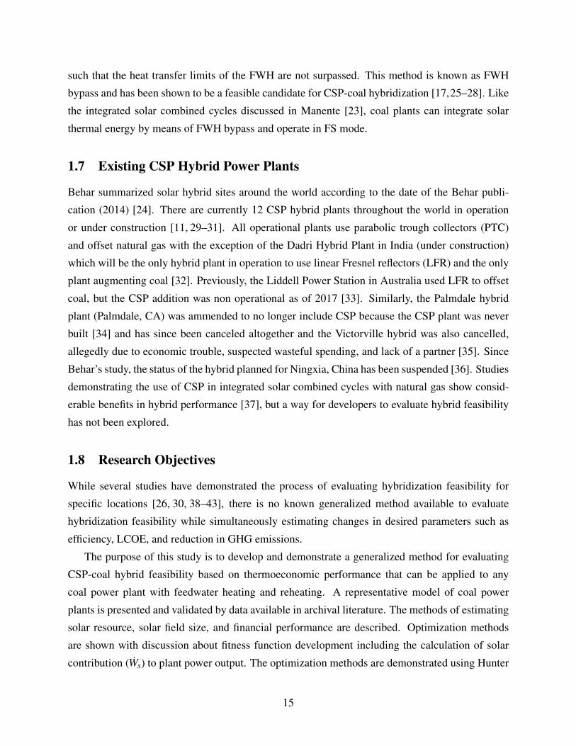
such that the heat transfer limits of the FWH are not surpassed. This method is known as FWH
bypass and has been shown to be a feasible candidate for CSP-coal hybridization [17,25–28]. Like
the integrated solar combined cycles discussed in Manente [23], coal plants can integrate solar
thermal energy by means of FWH bypass and operate in FS mode.
1.7 Existing CSP Hybrid Power Plants
Behar summarized solar hybrid sites around the world according to the date of the Behar publi-
cation (2014) [24]. There are currently 12 CSP hybrid plants throughout the world in operation
or under construction [11, 29–31]. All operational plants use parabolic trough collectors (PTC)
and offset natural gas with the exception of the Dadri Hybrid Plant in India (under construction)
which will be the only hybrid plant in operation to use linear Fresnel reflectors (LFR) and the only
plant augmenting coal [32]. Previously, the Liddell Power Station in Australia used LFR to offset
coal, but the CSP addition was non operational as of 2017 [33]. Similarly, the Palmdale hybrid
plant (Palmdale, CA) was ammended to no longer include CSP because the CSP plant was never
built [34] and has since been canceled altogether and the Victorville hybrid was also cancelled,
allegedly due to economic trouble, suspected wasteful spending, and lack of a partner [35]. Since
Behar’s study, the status of the hybrid planned for Ningxia, China has been suspended [36]. Studies
demonstrating the use of CSP in integrated solar combined cycles with natural gas show consid-
erable benefits in hybrid performance [37], but a way for developers to evaluate hybrid feasibility
has not been explored.
1.8 Research Objectives
While several studies have demonstrated the process of evaluating hybridization feasibility for
specific locations [26, 30, 38–43], there is no known generalized method available to evaluate
hybridization feasibility while simultaneously estimating changes in desired parameters such as
efficiency, LCOE, and reduction in GHG emissions.
The purpose of this study is to develop and demonstrate a generalized method for evaluating
CSP-coal hybrid feasibility based on thermoeconomic performance that can be applied to any
coal power plant with feedwater heating and reheating. A representative model of coal power
plants is presented and validated by data available in archival literature. The methods of estimating
solar resource, solar field size, and financial performance are described. Optimization methods
are shown with discussion about fitness function development including the calculation of solar
contribution (Ws) to plant power output. The optimization methods are demonstrated using Hunter
15
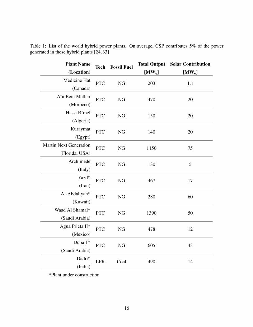
Table 1: List of the world hybrid power plants. On average, CSP contributes 5% of the powergenerated in these hybrid plants [24, 33]
Plant Name(Location)
Tech Fossil Fuel Total Output[MWe]
Solar Contribution[MWe]
Medicine Hat
(Canada)PTC NG 203 1.1
Aın Beni Mathar
(Morocco)PTC NG 470 20
Hassi R’mel
(Algeria)PTC NG 150 20
Kuraymat
(Egypt)PTC NG 140 20
Martin Next Generation
(Florida, USA)PTC NG 1150 75
Archimede
(Italy)PTC NG 130 5
Yazd*
(Iran)PTC NG 467 17
Al-Abdaliyah*
(Kuwait)PTC NG 280 60
Waad Al Shamal*
(Saudi Arabia)PTC NG 1390 50
Agua Prieta II*
(Mexico)PTC NG 478 12
Duba 1*
(Saudi Arabia)PTC NG 605 43
Dadri*
(India)LFR Coal 490 14
*Plant under construction
16

Unit 3 in Castle Dale, UT as a representative coal power plant. This study focuses primarily on
retrofit projects and is most related to fuel saving mode [23] to reduce the cost and complexity of
retrofitting a power plant with solar collectors while still increasing efficiency.
17
2 Methods
Each coal plant differs from the next, but several hardware components are common to most power
plant configurations. A representative plant model is developed that generally operates in a similar
way to most coal plants but with simplifications that make it applicable to most coal plants. The
solar integration model developed in this study, consisting of the representative plant and solar
exchange (SX) model, assumes the coal plant of interest has at least one FWH in the low pressure
(LP condensate stage and one FWH in the high pressure (HP) feedwater stage. Specific examples
are calculated based on data for the Hunter Unit 3 in Castle Dale, UT Provided by PacifiCorp and
validated where possible by data published in archival literature.
2.1 Power Plant Model
There are several power generation components that are consistently used in coal power plant
configurations:
• Multiple turbines (Typically high, intermediate, and low pressure turbines)
• High pressure feedwater heating (HP FWH) from high and intermediate pressure turbines’
(HPT and IPT, respectively) extraction and exhaust steam
• HPT exhaust reheating
• Low pressure feedwater heating (LP FWH) from low pressure turbine (LPT) extraction steam
2.1.1 Representative Plant Model
Each coal plant differs from the next, but several hardware components are common to most power
plant configurations. The Hunter 3 Unit includes all of the standard components identified in
the introduction. Data made available by PacifiCorp on the Hunter Unit performance provides a
reliable source to benchmark the representative model introduced in this report.
Justification for the plant simplification is provided below. First, the thermodynamic princi-
ples that allow the simplification are described. Then the methods used to extract or calculate
representative model inputs are explained. Finally, possible sources of error are discussed.
18

1
5
6
9
10
14
12
13
17
BFP
CP
4
3
1516
LPT
2
HP FWH
LP FWH
LPT
IPT
HPT
Condenser
7
8
11
BoilerReheater
Wnet
Figure 3: Schematic of the representative plant model analyzed in this study.
Combining Feedwater Heaters
As noted in Chapter 1, FWHs are common points of access for solar heating so attention is
given to modeling the FWH processes accurately. The major focus of the plant simplification
centered around reducing the number of FWHs and the amount of steam and the pressure at which
the steam is extracted to run the FWHs.
The FWHs used in the representative plant model are modeled as open FWHs, similar to those
found in published articles and in the Hunter heat balance diagram. The drain cooler (DC) is used
to fix the operating parameters in the representative plant model. The DC sets the temperature
19

difference between the drain outlet and the FWH inlet streams.
A mass-averaged approach is used to approximate the DC for both the HP and LP FWH. As a
sample case, consider a system of three LP FWHs that extract steam from the LPT at three different
pressures. The extraction mass flow rates are converted to percentages of the total mass of steam
extracted for that stage. Each LPT extraction is divided by the total mass flow rate from the three
LPT extraction streams to obtain mass fractions A, B, and C (where A+B+C=1). The overall DC
is determined by multiplying each mass fraction (A, B, and C) by its corresponding FWH DC and
adding the three mass fraction-DC products. If the hypothetical FWHs have a DC of 5 (stream
A), 7 (stream B), and 10 (stream C) °C, then the overall DC to be used in the representative plant
model would be DC = 5A+7B+10C. This process is repeated for the HP FWH overall DC and
both LP and HP DC.
It is efficient to incrementally heat the feedwater in multiple stages where the temperature of
the extracted steam increases alongside the increase in pressure stage. The pressure of the feed-
water ideally does not change significantly as it passes through each FWH. Each FWH can then
be modeled as a simplified, isobaric heating process. There are changes to the exergy destruc-
tion when the feedwater is not heated incrementally by progressively higher temperatures, but the
FWHs are modeled as a single heating process.
As can be seen in Choudhary [44], heat transfer devices (FWHs and boiler) are significant
sources of entropy generation, so reducing the number of and operating parameters for the FWHs
is expected to have a non-negligible impact on the overall entropy generated in the cycle and, con-
sequently, the 2nd law efficiency. This change in entropy generation will be captured in calculations
of Ws (Appendix A).
Boiler Feed Pump Turbine
The inlet and exhaust pressures of the boiler feed pump turbine (BFPT) are the same as the LPT
inlet and exhaust. Rather than modeling a branch from the IPT exhaust, the amount of steam that
would go through the BFPT is sent through the LPT. To compensate for the additional mass going
through the LPT, the power required for the BFP is added to the gross work output requirement
from the representative model.
Steam Extraction Selection
From the Hunter heat balance diagram and the Adibhatla and Kaushik schematic [28], all LP
FWHs use extracted steam from the LPT. The steam used for the LP FWH in the representative
20

model should be steam extracted from the LPT. The mass-averaged pressure of the extraction lines
in the Hunter plant is used as the extraction pressure in the representative model. More detail about
how the mass-average method is applied to calculate the extraction steam pressure is presented in
Appendix B.
The HP FWHs in coal plants use varying combinations of steam extracted from both the HPT
and IPT. The representative model assumes that the HP FWH uses steam extracted from the HPT
exhaust before the reheat process and is throttled to the mass-averaged pressure. The inclusion
of the throttling valve adds entropy generation unique to the representative model. Compared to
modeling the HP FWH steam as extraction from the IPT in the representative model, throttling the
HPT exhaust to the mass-averaged pressure was selected to achieve model accuracy and preserve
simplicity. More details on the decision between modeling the HP FWH extraction is provided in
Appendix C.
The efficiency of each turbine is also determined using the mass-averaged approach between
the inlet pressure and each extraction and exhaust pressure. The mass-averaged efficiency and
the pressures discussed above are sufficient to determine the other fluid properties throughout the
cycle. The methods of calculating each individual state point for the representative model are
provided in Appendix B.
Representative Model Simulation
Coal power plants control the total power generation of the cycle by adjusting the HPT 1st
stage pressure (Ps1) and the working fluid mass flow rate. The representative model was modified
to calculate the plant performance, limited by a maximum power output constraint, when allowing
bypass of a single FWH by solar heating (i.e. solar bypass). After simulating the turbine power
generation with the recalculated extraction pressure, power output constraints for the overall plant
and each individual turbine can be compared to the respective calculated values. If a constraint is
violated, Ps1 is incrementally reduced by 5% until all constraints are satisfied.
Changing Ps1 has downstream effects on the mass flow rate, boiler operating temperature, and
pressure ratios between the inlet to a turbine and each respective extraction or exhaust stream.
Relationships between Ps1 and each operating property must be determined and included in the
model. Specifically, the properties for which a correlation is required include:
• Condenser pressure
• All FWH extraction pressure ratios
• Boiler inlet pressure
21

• Boiler outlet pressure
• Boiler operating temperature
• Boiler inlet mass flow rate
• Deaerator (DA) inlet water mass flow rate
• Extraction fractions for each FWH
• HPT, IPT, LPT isentropic efficiencies
• IPT, LPT extraction pressure ratios
Specific correlations for each property listed above are provided in Table F.1 along with a
detailed description of how each state point is calculated in Appendix B.
2nd Law Efficiency
The 2nd Law Efficiency (ηII) is a value that quantifies the ability of a process to convert its
work potential into useful work. Calculating ηII requires assuming a dead state, or the conditions
at which no further work can be performed. For this analysis, the dead state temperature is assumed
to be equivalent to the saturation temperature inside the condenser. The advantages of this choice
will be clarified after the efficiency model is developed.
PowerPlant
QB
Wnet
Qout
TB
T0
Qs
Tsun
Figure 4: Simplified heat engine schematic. The system of interest is enclosed by the dashed circle.
Figure 4 shows a simplified heat engine schematic with arrows indicating the exergy interac-
tions that cross the dashed boundary of the power plant: the heating done in the boiler, the net
power output, and the energy rejected in the condenser as well as the energy rejected due to ineffi-
ciencies in the plant hardware.
The exergy rate for net power out (XW ) is equal to the net power out of the cycle (Equation 1).
22
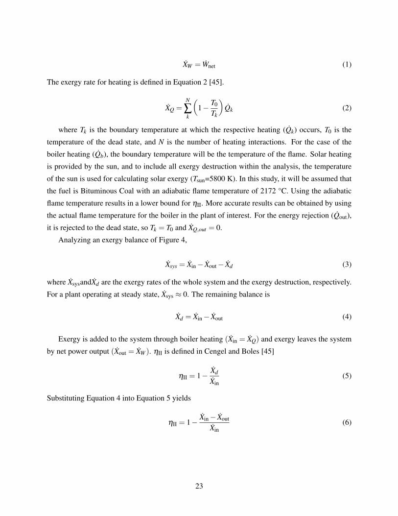
XW = Wnet (1)
The exergy rate for heating is defined in Equation 2 [45].
XQ =N
∑k
Å1− T0
Tk
ãQk (2)
where Tk is the boundary temperature at which the respective heating (Qk) occurs, T0 is the
temperature of the dead state, and N is the number of heating interactions. For the case of the
boiler heating (Qb), the boundary temperature will be the temperature of the flame. Solar heating
is provided by the sun, and to include all exergy destruction within the analysis, the temperature
of the sun is used for calculating solar exergy (Tsun=5800 K). In this study, it will be assumed that
the fuel is Bituminous Coal with an adiabatic flame temperature of 2172 °C. Using the adiabatic
flame temperature results in a lower bound for ηII. More accurate results can be obtained by using
the actual flame temperature for the boiler in the plant of interest. For the energy rejection (Qout),
it is rejected to the dead state, so Tk = T0 and XQ,out = 0.
Analyzing an exergy balance of Figure 4,
Xsys = Xin− Xout− Xd (3)
where XsysandXd are the exergy rates of the whole system and the exergy destruction, respectively.
For a plant operating at steady state, Xsys ≈ 0. The remaining balance is
Xd = Xin− Xout (4)
Exergy is added to the system through boiler heating (Xin = XQ) and exergy leaves the system
by net power output (Xout = XW ). ηII is defined in Cengel and Boles [45]
ηII = 1− Xd
Xin(5)
Substituting Equation 4 into Equation 5 yields
ηII = 1− Xin− Xout
Xin(6)
23
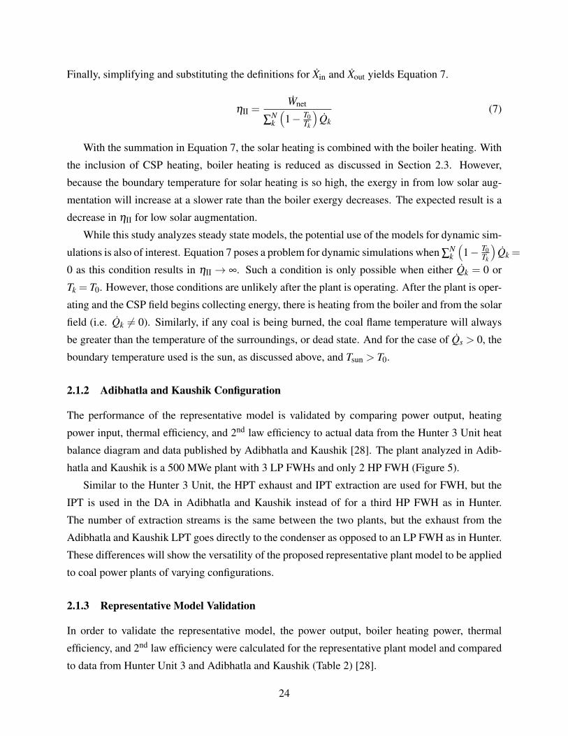
Finally, simplifying and substituting the definitions for Xin and Xout yields Equation 7.
ηII =Wnet
∑Nk
Ä1− T0
Tk
äQk
(7)
With the summation in Equation 7, the solar heating is combined with the boiler heating. With
the inclusion of CSP heating, boiler heating is reduced as discussed in Section 2.3. However,
because the boundary temperature for solar heating is so high, the exergy in from low solar aug-
mentation will increase at a slower rate than the boiler exergy decreases. The expected result is a
decrease in ηII for low solar augmentation.
While this study analyzes steady state models, the potential use of the models for dynamic sim-
ulations is also of interest. Equation 7 poses a problem for dynamic simulations when ∑Nk
Ä1− T0
Tk
äQk =
0 as this condition results in ηII → ∞. Such a condition is only possible when either Qk = 0 or
Tk = T0. However, those conditions are unlikely after the plant is operating. After the plant is oper-
ating and the CSP field begins collecting energy, there is heating from the boiler and from the solar
field (i.e. Qk 6= 0). Similarly, if any coal is being burned, the coal flame temperature will always
be greater than the temperature of the surroundings, or dead state. And for the case of Qs > 0, the
boundary temperature used is the sun, as discussed above, and Tsun > T0.
2.1.2 Adibhatla and Kaushik Configuration
The performance of the representative model is validated by comparing power output, heating
power input, thermal efficiency, and 2nd law efficiency to actual data from the Hunter 3 Unit heat
balance diagram and data published by Adibhatla and Kaushik [28]. The plant analyzed in Adib-
hatla and Kaushik is a 500 MWe plant with 3 LP FWHs and only 2 HP FWH (Figure 5).
Similar to the Hunter 3 Unit, the HPT exhaust and IPT extraction are used for FWH, but the
IPT is used in the DA in Adibhatla and Kaushik instead of for a third HP FWH as in Hunter.
The number of extraction streams is the same between the two plants, but the exhaust from the
Adibhatla and Kaushik LPT goes directly to the condenser as opposed to an LP FWH as in Hunter.
These differences will show the versatility of the proposed representative plant model to be applied
to coal power plants of varying configurations.
2.1.3 Representative Model Validation
In order to validate the representative model, the power output, boiler heating power, thermal
efficiency, and 2nd law efficiency were calculated for the representative plant model and compared
to data from Hunter Unit 3 and Adibhatla and Kaushik (Table 2) [28].
24

Figure 5: Schematic for the power plant analyzed in Adibhatla and Kaushik [28]
WWW net
[MW]QQQin
[MW]ηηη ttthhh
[%]ηηη IIIIII
[%]
Hun
ter Reported Cycle Performance 511 1273 37.3 46.1
Representative Model 505 1276 39.6 45.1
Change (%) -1.2 0.2 6.2 -2.2
Adi
bhat
la&
Kau
shik Reported Cycle Performance 500 1300 38.5 44.2
Representative Model 511 1332 38.3 43.7
Change (%) 2.2 2.5 -0.4 -1.1
Table 2: Results of applying the representative plant model to the Hunter 3 Unit and the dataprovided in Adibhatla and Kaushik [28].
The largest error is in the thermal efficiency. The thermal efficiency error likely stems from
using mass-averaged values and other simplifications listed in this report. Using mass-averaged
values approximates the changes in turbine efficiency with flow rate which affects the reported
power output. Assuming constant pressure through FWH stages also reduces the power required
by the CP and BFP. However, the net power output error is consistent between the two examples, so
altering input parameters, e.g. solar augmentation, should have a consistent effect on the reported
net power output. The boiler heating model is more accurate and will closely approximate the
heating load on the system and corresponding emissions reduction from solar augmentation.
25

It is important to also note how the representative model compares to Hunter and Adibhatla and
Kaushik’s data for the entire cycle in addition to the parameters outlined in Table 2. More accurate
approximations of the power plant in Adibhatla and Kaushik may be attainable with operating
data similar to the data made available for the Hunter Unit 3. Figure 6 shows the comparison of
the predicted state points from the representative model with the Hunter Unit 3 (Figure 6a) and
Adibhatla and Kaushik (Figure 6b). The representative model sacrifices some accuracy to achieve
consistency in modeling power plants with different configurations. Thus, results for this study will
be obtained by varying the amount of solar augmentation to produce results that can be compared
to each other based on changes in fuel consumption
0 2 4 6 8 10
Entropy [kJ kg-1
K-1
]
200
300
400
500
600
700
800
900
Te
mp
era
ture
[K
]
Saturated Water Dome
Hunter Main Loop
Representative Model Main Loop
(a)
0 2 4 6 8 10
Entropy [kJ kg-1
K-1
]
200
300
400
500
600
700
800
900
Te
mp
era
ture
[K
]
Saturated Water Dome
Adibhatla and Kaushik Main Loop
Representative Model Main Loop
(b)
Figure 6: T-s diagrams comparing the performance of the representative model with (a) Hunter 3Unit and (b) data in Adibhatla and Kaushik [28].
One notable difference is the discrepancy between the temperature of the mass entering the
condenser of the Hunter Unit, located at the bottom right of the cycle diagram in Figure 6a. The
data used to define the Hunter Unit main loop is obtained directly from the heat balance diagram.
The Hunter operating data suggests the LPT exhaust is actually at a lower pressure than is reported
on the diagram. Using experimental data for the LPT exhaust would improve the Hunter com-
parison in Figure 6a. The error in power output can be seen in Figures 6 by the space between
the vertical lines on the far right of each diagram denoting the IPT and LPT processes. As noted
above, the error in estimates of power generation is expected when mass-averaged values are used
for efficiencies. The Wnet error is compounded as the same method of using mass avergaed values
is applied to all turbines. However, the actual plant and respective model diagrams match well and
appear to be consistent, regardless of plant configuration.
26

2.2 Solar Resource
The amount of solar resource available per unit area is referred to in this study as the direct normal
insolation (DNI). Since DNI is susceptible to fluctuations due to weather, the maximum possible
DNI for a given time is based on calculations for a clear sky (CSDNI), such that DNI≤CSDNI.
The following sections describe methods to estimate the expected DNI at any given geography and
its use in the SX model.
2.2.1 NSRDB Data
The National Renewable Energy Laboratory (NREL) reports solar resource data in the National
Solar Resource Database (NSRDB) [46] for a number of locations in the United States, Canada,
and South America. Sengupta et al. describes the method of retrieving data from the online NSRDB
data viewer in depth [47]. The NSRDB has data from several meteorological measurements. For
the methods described in Section 2.2.2, DNI [W m-2], CSDNI [W m-2], solar zenith angle (θz)
[degrees], temperature [°C], and pressure [mbar] are utilized.
2.2.2 Solar Data Processing
A MATLAB script (Appendix H.4) has been written to process data downloaded from the NSRDB
as described below. The average DNI for each day is calculated according to Equation 8 where
N is the number of possible daylight data points. N is determined for each day by counting the
number of data points for which CSDNI>0.
DNIavg =1N
N
∑i=1
DNIi (8)
Once the daily average is calculated for each day in the year file, the script then opens the next
file, calculates daily averages and adds the averages from the currently open file to the sum of
the average values from the previous files. Dividing the data array by the number of data files
(or number of years) provides the multiple year daily average for each parameter. The multiple
year daily averages are then averaged to generate the total multi-year average. When the multi-
year average DNI is multiplied by the multi-year average daylight time (N), the multi-year average
solar energy is calculated.
For Castle Dale, UT, the calculated multi-year average DNI and daylight time are 542 W m-2
and 11.9 h, respectively. The calculated value for multi-year average solar energy then is 6.45 kWh
m-2. The NSRDB reports 6.48 kWh m-2 as the nominal energy flux value for Castle Dale, UT. The
27
Nl
1
2
Module
SCA
Na1 2
Ts,in Ts,out
w
p
Lr
LSCA
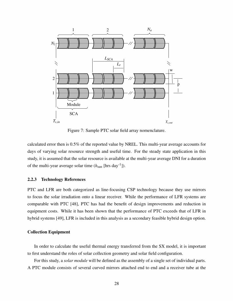
Figure 7: Sample PTC solar field array nomenclature.
calculated error then is 0.5% of the reported value by NREL. This multi-year average accounts for
days of varying solar resource strength and useful time. For the steady state application in this
study, it is assumed that the solar resource is available at the multi-year average DNI for a duration
of the multi-year average solar time (hsun [hrs day-1]).
2.2.3 Technology References
PTC and LFR are both categorized as line-focusing CSP technology because they use mirrors
to focus the solar irradiation onto a linear receiver. While the performance of LFR systems are
comparable with PTC [48], PTC has had the benefit of design improvements and reduction in
equipment costs. While it has been shown that the performance of PTC exceeds that of LFR in
hybrid systems [49], LFR is included in this analysis as a secondary feasible hybrid design option.
Collection Equipment
In order to calculate the useful thermal energy transferred from the SX model, it is important
to first understand the roles of solar collection geometry and solar field configuration.
For this study, a solar module will be defined as the assembly of a single set of individual parts.
A PTC module consists of several curved mirrors attached end to end and a receiver tube at the
28
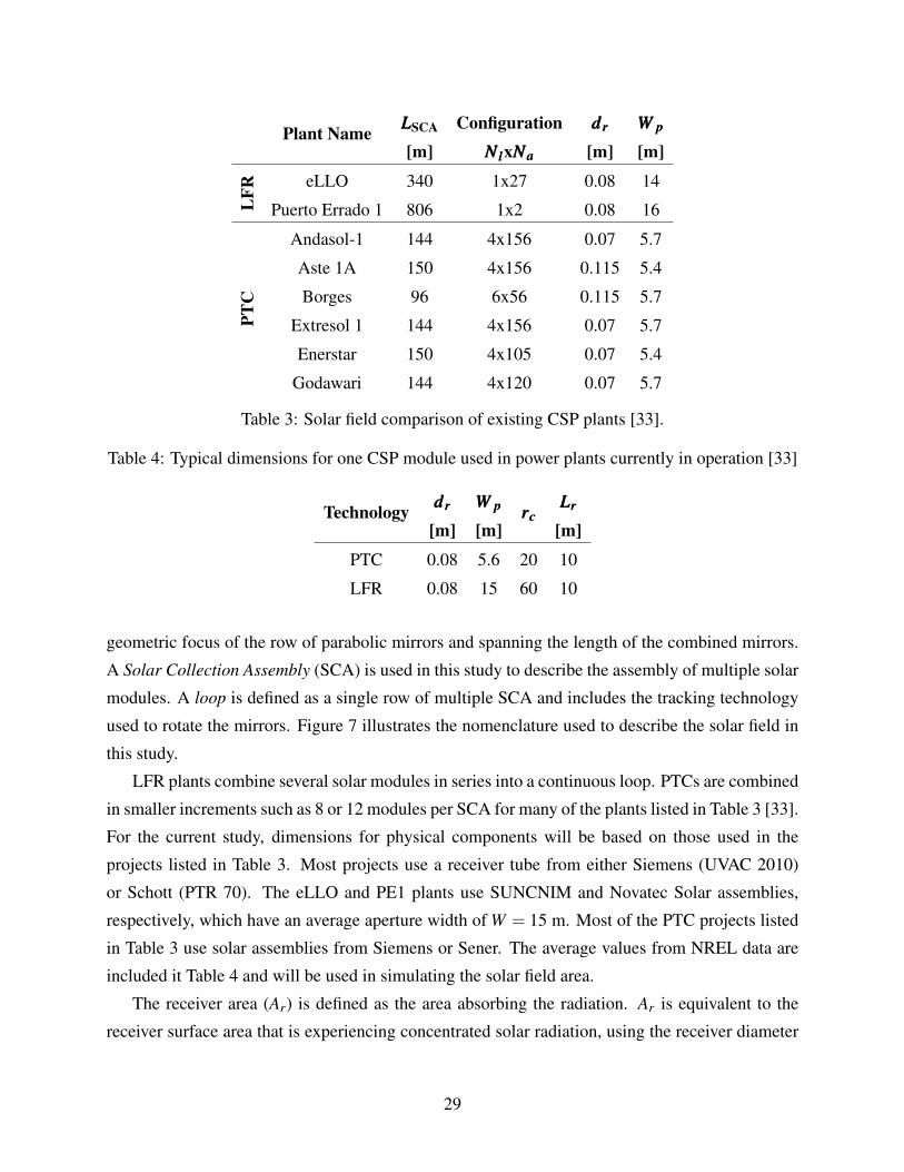
Plant Name LLLSCA
[m]Configuration
NNNlllxNNNaaa
dddrrr
[m]WWW ppp
[m]
LFR
eLLO 340 1x27 0.08 14
Puerto Errado 1 806 1x2 0.08 16
PTC
Andasol-1 144 4x156 0.07 5.7
Aste 1A 150 4x156 0.115 5.4
Borges 96 6x56 0.115 5.7
Extresol 1 144 4x156 0.07 5.7
Enerstar 150 4x10⁵ 0.07 5.4
Godawari 144 4x120 0.07 5.7
Table 3: Solar field comparison of existing CSP plants [33].
Table 4: Typical dimensions for one CSP module used in power plants currently in operation [33]
Technology dddrrr
[m]WWW ppp
[m]rrrccc
LLLrrr
[m]
PTC 0.08 5.6 20 10
LFR 0.08 15 60 10
geometric focus of the row of parabolic mirrors and spanning the length of the combined mirrors.
A Solar Collection Assembly (SCA) is used in this study to describe the assembly of multiple solar
modules. A loop is defined as a single row of multiple SCA and includes the tracking technology
used to rotate the mirrors. Figure 7 illustrates the nomenclature used to describe the solar field in
this study.
LFR plants combine several solar modules in series into a continuous loop. PTCs are combined
in smaller increments such as 8 or 12 modules per SCA for many of the plants listed in Table 3 [33].
For the current study, dimensions for physical components will be based on those used in the
projects listed in Table 3. Most projects use a receiver tube from either Siemens (UVAC 2010)
or Schott (PTR 70). The eLLO and PE1 plants use SUNCNIM and Novatec Solar assemblies,
respectively, which have an average aperture width of W = 15 m. Most of the PTC projects listed
in Table 3 use solar assemblies from Siemens or Sener. The average values from NREL data are
included it Table 4 and will be used in simulating the solar field area.
The receiver area (Ar) is defined as the area absorbing the radiation. Ar is equivalent to the
receiver surface area that is experiencing concentrated solar radiation, using the receiver diameter
29
(dr) and length (Lr) [50].
Ar = πdrLr (9)
For LFR systems, the receiver is often covered from above by a trapezoidal reflector (shown
in Figure 1b) to focus the thermal radiation onto the entire receiver. However, receivers on PTC
modules do not absorb concentrated radiation through areas outside the focal area, or the area
onto which thermal radiation is concentrated. The focal area depends on the aperture width and
curvature of the PTC mirrors. To simplify the analysis in this report, the focal area of PTC modules
will be assumed to be approximately equal to Ar, noting that the actual thermal energy collected
over this area will be slightly less and accounted for when simulating the configuration of the solar
field.
Aperture area (Ap) is defined as the area through which radiation enters the collector. In the case
of PTC, Ap is the projected area of the mirror calculated by the product of Lr and the perpendicular
opening width (Wp). The Ap for LFR would be the product of the length of each mirror and the
width of the overall mirror array.
The goal of CSP technology is to maximize the ratio between Ap and Ar, or concentration ratio
(Equation 10).
rc =Ap
Ar(10)
If Ar is 50 times smaller than Ap, the heat flux absorbed by the receiver (q′′r ) would be 50 times
greater than the solar heat flux (DNI) entering the aperture area (Equation 11).
q′′r = rcDNI (11)
Heat Transfer Fluid
CSP systems require a HTF to be pumped through the collection vessel and often use a heat
exchanger to move the absorbed thermal energy for use elsewhere. Typical HTFs include air, water,
molten solar salts (i.e. NaNO3, KNO3, etc. [51]), and thermal oils.
Air is a useful HTF due to its availability and versatility. While air does have a lower thermal
capacitance compared to the other HTF in Table 5, it also avoids complications associated with
phase change. The gas properties of air (including viscosity in Table 5) make it much easier to
pump through a CSP system or compress to allow for a greater change in temperature. The thermal
properties reported in Table 5 are largely what limit the application of air as a HTF. The specific
heat of air is comparable to the other HTFs but for the same temperature difference, the volume of
30
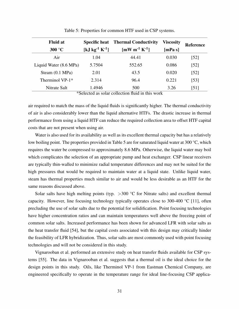
Table 5: Properties for common HTF used in CSP systems.
Fluid at300 °C
Specific heat[kJ kg-1 K-1]
Thermal Conductivity[mW m-1 K-1]
Viscosity[mPa s]
Reference
Air 1.04 44.41 0.030 [52]
Liquid Water (8.6 MPa) 5.7504 552.65 0.086 [52]
Steam (0.1 MPa) 2.01 43.5 0.020 [52]
Therminol VP-1* 2.314 96.4 0.221 [53]
Nitrate Salt 1.4946 500 3.26 [51]*Selected as solar collection fluid in this work
air required to match the mass of the liquid fluids is significantly higher. The thermal conductivity
of air is also considerably lower than the liquid alternative HTFs. The drastic increase in thermal
performance from using a liquid HTF can reduce the required collection area to offset HTF capital
costs that are not present when using air.
Water is also used for its availability as well as its excellent thermal capacity but has a relatively
low boiling point. The properties provided in Table 5 are for saturated liquid water at 300 °C, which
requires the water be compressed to approximately 8.6 MPa. Otherwise, the liquid water may boil
which complicates the selection of an appropriate pump and heat exchanger. CSP linear receivers
are typically thin-walled to minimize radial temperature differences and may not be suited for the
high pressures that would be required to maintain water at a liquid state. Unlike liquid water,
steam has thermal properties much similar to air and would be less desirable as an HTF for the
same reasons discussed above.
Solar salts have high melting points (typ. >300 °C for Nitrate salts) and excellent thermal
capacity. However, line focusing technology typically operates close to 300-400 °C [11], often
precluding the use of solar salts due to the potential for solidification. Point focusing technologies
have higher concentration ratios and can maintain temperatures well above the freezing point of
common solar salts. Increased performance has been shown for advanced LFR with solar salts as
the heat transfer fluid [54], but the capital costs associated with this design may critically hinder
the feasibility of LFR hybridization. Thus, solar salts are most commonly used with point focusing
technologies and will not be considered in this study.
Vignarooban et al. performed an extensive study on heat transfer fluids available for CSP sys-
tems [55]. The data in Vignarooban et al. suggests that a thermal oil is the ideal choice for the
design points in this study. Oils, like Therminol VP-1 from Eastman Chemical Company, are
engineered specifically to operate in the temperature range for ideal line-focusing CSP applica-
31

tions [53]. While the thermal properties of oils are less impressive when compared to liquid water
or solar salts, thermal oils are most often used due to their stability in typical line-focusing tem-
perature ranges. For this study, properties for Therminol VP-1 will be used for solar collection
calculations.
2.2.4 Solar Field Simulation
While the concentration ratio is determined by the installed hardware, the length used for collection
can be adjusted. However, a straight line of CSP collectors for several miles is often not desirable
so collectors are placed in arrays. For Nl loops of collection, the equation for the thermal power
absorbed by the solar field (qabs, f ) can be related to collection geometry using Equation 12.
qabs, f = NlrcDNIAr (12)
Alternatively, qabs, f can also be calculated using the change in temperature (∆Ts) and specific
heat (cp,s) of the solar heat transfer fluid (Equation 13) assuming the fluid does not undergo a phase
change.
qabs, f = mscp,s∆Ts (13)
The solar heat transfer fluid can then be routed to each collector either in parallel or in series. Series
flow assumes that, even if the collectors are in an array, the mass flow rate is constant throughout
each loop and the fluid is routed in a serpentine manner. Parallel flow assumes that a uniform
fraction of mass flow rate is divided among each loop and mixes at the end before entering the
solar heat exchanger. For the case of a CSP array with Nl loops, Equation 12 can be altered such
that
qr = rcDNIηc
Nl
∑i=1
Ar,i (14)
where Ar,i is the receiver area for the ith loop and ηc is the overall collection efficiency of the SCA.
If each loop is assumed to be uniform (i.e. uniform length, mass flow), then Equation 14 can be
further simplified and combined with Equation 13 (where ml =msNl
).
qr = NlrcDNIηcAr,l = Nlmlcp,s∆Ts (15)
From Equation 15 it can be seen that ∆Ts will be less for parallel flow. To achieve the same
qabs, f , the total mass flow rate must be larger than in series. The large ∆Ts that can be expected in
32
a series configuration is not desirable if the process is operating close to the boiling point of the
heat transfer fluid. Large temperature gradients may also cause warping in receiver tubes that can
result in the defocusing of the receiver and radiation leakage.
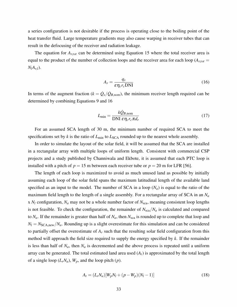
The equation for Ar,tot can be determined using Equation 15 where the total receiver area is
equal to the product of the number of collection loops and the receiver area for each loop (Ar,tot =
NlAr,l).
Ar =qs
εηcrcDNI(16)
In terms of the augment fraction (k = Qs/QB,nom), the minimum receiver length required can be
determined by combining Equations 9 and 16
Lmin =kQB,nom
DNI εηcrcπdr(17)
For an assumed SCA length of 30 m, the minimum number of required SCA to meet the
specifications set by k is the ratio of Lmin to LSCA rounded up to the nearest whole assembly.
In order to simulate the layout of the solar field, it will be assumed that the SCA are installed
in a rectangular array with multiple loops of uniform length. Consistent with commercial CSP
projects and a study published by Channiwala and Ekbote, it is assumed that each PTC loop is
installed with a pitch of p = 15 m between each receiver tube or p = 20 m for LFR [56].
The length of each loop is maximized to avoid as much unused land as possible by initially
assuming each loop of the solar field spans the maximum latitudinal length of the available land
specified as an input to the model. The number of SCA in a loop (Na) is equal to the ratio of the
maximum field length to the length of a single assembly. For a rectangular array of SCA in an Na
x Nl configuration, Na may not be a whole number factor of Nsca, meaning consistent loop lengths
is not feasible. To check the configuration, the remainder of Nsca/Na is calculated and compared
to Na. If the remainder is greater than half of Na, then Nsca is rounded up to complete that loop and
Nl = NSCA,new/Na. Rounding up is a slight overestimate for this simulation and can be considered
to partially offset the overestimate of Ar such that the resulting solar field configuration from this
method will approach the field size required to supply the energy specified by k. If the remainder
is less than half of Na, then Na is decremented and the above process is repeated until a uniform
array can be generated. The total estimated land area used (At) is approximated by the total length
of a single loop (LrNa), Wp, and the loop pitch (p).
At = (LrNa)[WpNl +(p−Wp)(Nl−1)] (18)
33

Table 6: Effect of technology and maximum loop length (Ll,max) on receiver area (Ar) and solarfield size (Asf)
LLLlll,,,mmmaaaxxx
[m]kkk
[%]Technology AAArrr
[103 m2]AAAsss fff
[ac]
300
1PTC 2.1 30.4
LFR 1.1 21.1
6PTC 12.4 182.8
LFR 6.5 127
10PTC 20.7 305.1
LFR 10.8 211.4
500
1PTC 2.1 30.2
LFR 1.1 21.6
6PTC 12.4 182.2
LFR 6.5 127.2
10PTC 20.8 305
LFR 10.8 210.8
1000
1PTC 2.2 29.8
LFR 1.2 22.3
6PTC 12.4 181.2
LFR 6.5 127.2
10PTC 20.8 303.9
LFR 10.8 211.3
The effect of maximum loop length (Ll,max) and k on the amount of receiver area and the size
of the total solar field for both PTC and LFR is shown in Table 6. There does not appear to be
a significant effect of Ll,max on Ar. For most instances, increasing Ll,max reduces Asf, which is
expected due to the potential reduction in total number of loops and unused land due to spacing
needs. However, the changes in Asf from Ll,max are not significant, so the estimates of Asf from this
analysis are largely independent of the geometry of the land designated for the solar field.
2.3 Solar Integration Model
Thermal energy collected by the solar field is assumed to be integrated into the coal power block
by means of FWH bypass. The water bypasses the designated FWH and instead passes through
34

a different heat exchanger in which the solar thermal energy is transferred to the water. Because
the CSP energy is replacing the role of steam extracted from a turbine, that extraction mass flow
is then assumed to continue through the cycle, increasing the total inlet enthalpy of the applicable
turbine and all downstream hardware. Increasing the total enthalpy in turn increases the total
power generated by each turbine. However, the simplified coal model used in this study assumes
the FWH process is done by a single FWH at constant pressure. These changes in the power block
thermodynamics require an update to the simplified model to allow for single FWH bypass and
limits to total power generation.
The steam extraction pressure is calculated using the mass-averaged pressure approach assum-
ing all flow rates are unchanged with the exception of the extraction line tied to the bypassed
FWH and the main line. In the solar integration model, this is illustrated by placing the solar heat
exchanger (SX) in series before the constant pressure FWH (Options A and C in Figure 8) with
thermal input from the solar field to the SX if the FWH being bypassed is followed by another
FWH in the real cycle. For FWHs not followed by another FWH (i.e. before the boiler or BFP,
as in Options B and D in Figure 8), the SX was modeled after the combined FWH in the repre-
sentative model. State 4 (Figure 8) represents the mixing done in the DA. While the DA may be
thought of as an open FWH, only closed FWHs are considered as candidates for solar integration.
However, the FWH numbering scheme common to coal power plant schematics is preserved in
this study and FWH 4 is omitted from FWH bypass results discussed in Section 3.
2.4 Solar Contribution
Hou et al. defined a method to calculate the solar work contribution, Ws, that involved an exergy
analysis on subsystems of the overall hybrid plant [57]. An adaptation of their approach for the
solar integration model is presented here.
Subsystem boundary lines are selected based on the pressure level of the turbine stage included
in the subsystem as shown in Figure 9a with extraction and exhaust pressures. However since
steam is not extracted from the IP turbine, the boundary line corresponds with the pressure at state
13. Figure 9b illustrates the boundary lines for each subsystem when plotted on a T-s diagram
and shows the highlighted area under the subsystems which is integrated to calculate Ws. Each
subsystem remains consistent across multiple solar integration configurations (Options A-D in
Figure 3). The only modification is the inclusion of the SX model in different subsystems as the
integration location changes. For example, Subsystem 4 always contains the lower stages of the
LPT, the Condenser, CP, and drain cooler throttling after the LP FWH. For the lowest pressure
solar integration (Figure 9a), the SX occurs before LP FWH and splits that boundary between
35
1
5
6
9
10
14
12
13
17
BFP
CP
4
3
1516
LPT
2
HP FWH
LP FWH
LPT
IPT
HPT
Condenser
7
8
11
BoilerReheater
Wnet
2s
A
B
C
D
Ts,
out
T s,in
SX
SX Model
Representative Model
DNI
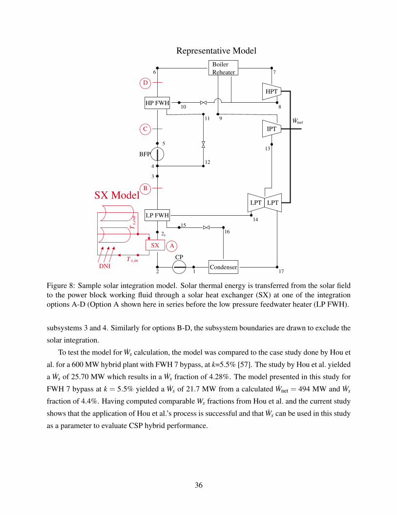
Figure 8: Sample solar integration model. Solar thermal energy is transferred from the solar fieldto the power block working fluid through a solar heat exchanger (SX) at one of the integrationoptions A-D (Option A shown here in series before the low pressure feedwater heater (LP FWH).
subsystems 3 and 4. Similarly for options B-D, the subsystem boundaries are drawn to exclude the
solar integration.
To test the model for Ws calculation, the model was compared to the case study done by Hou et
al. for a 600 MW hybrid plant with FWH 7 bypass, at k=5.5% [57]. The study by Hou et al. yielded
a Ws of 25.70 MW which results in a Ws fraction of 4.28%. The model presented in this study for
FWH 7 bypass at k = 5.5% yielded a Ws of 21.7 MW from a calculated Wnet = 494 MW and Ws
fraction of 4.4%. Having computed comparable Ws fractions from Hou et al. and the current study
shows that the application of Hou et al.’s process is successful and that Ws can be used in this study
as a parameter to evaluate CSP hybrid performance.
36
1
5
6
9
10
14
12
13
17
BFP
CP
4
3
1516
LPT
2
HP FWH
LP FWH
LPT
IPT
HPT
Condenser
7
8
11
BoilerReheater
Wnet
2s
T s,o
ut
Ts,in
SX Subsystem 4
Subsystem 3
Subsystem 2
Subsystem 1
DNI
(a)
0 2 4 6 8
Entropy [kJ kg-1
K-1
]
300
400
500
600
700
800
900
Te
mp
era
ture
[K
]
Subsystem 1
Subsystem 3
Subsystem 4
Solar ContributionVapor DomeMain LoopSubsystem Boundary
Subsystem 2
(b)
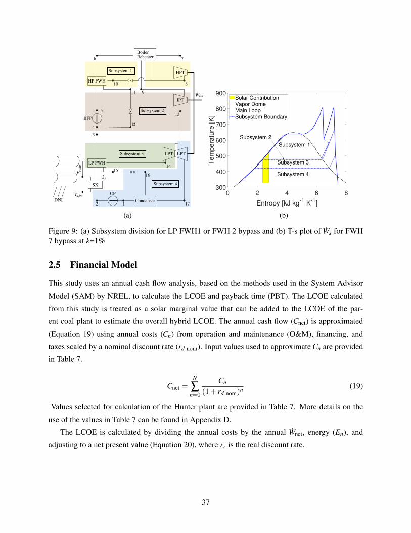
Figure 9: (a) Subsystem division for LP FWH1 or FWH 2 bypass and (b) T-s plot of Ws for FWH7 bypass at k=1%
2.5 Financial Model
This study uses an annual cash flow analysis, based on the methods used in the System Advisor
Model (SAM) by NREL, to calculate the LCOE and payback time (PBT). The LCOE calculated
from this study is treated as a solar marginal value that can be added to the LCOE of the par-
ent coal plant to estimate the overall hybrid LCOE. The annual cash flow (Cnet) is approximated
(Equation 19) using annual costs (Cn) from operation and maintenance (O&M), financing, and
taxes scaled by a nominal discount rate (rd,nom). Input values used to approximate Cn are provided
in Table 7.
Cnet =N
∑n=0
Cn
(1+ rd,nom)n (19)
Values selected for calculation of the Hunter plant are provided in Table 7. More details on the
use of the values in Table 7 can be found in Appendix D.
The LCOE is calculated by dividing the annual costs by the annual Wnet, energy (En), and
adjusting to a net present value (Equation 20), where rr is the real discount rate.
37

Table 7: Selected input values used for the cash flow cost analysis
Parameter Name Variable Selected Input Source
Capital CostSite Improvements FSI [USD m-2] 25 [58]
Solar Field FSF [USD m-2] 170 [58]
Heat Transfer Fluid FHTF [USD m-2] 60 [58]
Heat Exchanger FHX [MMUSD] 1.73 [59]
Contingency rcont [%] 7 [58]
Engineer-Procure-Construct rEPC [%] 11 [58]
Sales Tax Amount Ft,sal [% of CC] 80 [58]
Sales Tax Rate rt,sal [%] 5 [58]
Annual Operating ExpensesFixed O&M FFOM [USD kWe
-1] 12 [60]
Variable O&M FVOM [USD MWh-1] 4 [61]
Property Tax Amount Ft,prp [% of CC] 80 [61]
Property Tax Rate rt,prp [% of basis] 0.6 [62]
Insurance Rate rins [% of CC] 0.5 [61]
Annual Loan PaymentLoan Amount FL [% of CC] 50 [63]
Total Loan Period P [years] 25 [61]
Loan Interest Rate rint [% of remaining balance] 5 [61]
Annual Tax Credits and IncentivesFederal ITC Rate rITC,fed [% of CC] 10* [64]
State ITC Rate rITC,st [% of CC] 0 [61]
Annual State and Federal Income TaxDepreciation Schedule SCdep [% of CC] MACRS** [61]
Federal Tax Rate rt,Fed [%] 21 [61]
State Tax Rate rt,st| [%] 5 [62]
*rITC was set in 2019 to depreciate from 30% to 10% by 2022 [64].**The modified accelerated cost recovery system (MACRS) is the name given to the federaldepreciation schedule and has a separate value for the first five years of the project as shown inthe following vector (20, 32, 19.2, 11.52, 11.52, 5.76).
38

LCOE =Cnet
N∑
n=1
En(1+rr)
n
(20)
O&M, tax costs, and loan payments are approximated using values shown in Table 7. Informa-
tion on how to use the values in Table 7 is provided in Appendix D.
Two PBTs were calculated for this study. PBT1, used for the current analysis, assumes that
the fuel savings resulting from operating a hybrid plant in fuel saving mode provide the benefit
that offsets all accumulated costs inherent in the hybridization process. PBT2, discussed further
in Appendix D, assumes that the fuel savings provide the benefit that offsets only the initial in-
vestment. The fuel savings are calculated using the fuel offset and the lower heating value of the
coal (Equation 21). Annual fuel savings are subtracted from the annual costs until the savings are
greater than or equal to the cumulative costs.
FS =EsavFF
LHVF(21)
The development of this financial model closely reflects the calculations performed within
SAM by NREL; comparative tests during development showed agreement between the models to
the order of rounding error. Savings obtained from fuel offset is a departure from the scope of
SAM. The effect of augmentation and integration site on LCOE and PBT1 are explored further in
Section 3.2.
Carbon tax is an incentive that has been introduced in certain countries and areas of the US to
boost renewable energy projects over fossil fuel projects by penalizing the emission of greenhouse
gases [65]. Though not widely implemented in the US, hypothetical values for a carbon tax are
publicly available [66]. In this work, the effect of the carbon tax income is calculated from Qfo
and the useful solar operating conditions. Results from the implementation of a solar premium and
carbon tax are provided in Section 3.2.
Another option for improving financial feasibility is the consideration of a premium rate applied
to the electricity consumer. A study by O’Shaughnessy et al. states that the average green energy
premium paid by residential electricity consumers in 2016 was 0.018 USD kWh-1 [67]. In this
study, the income from increasing the electricity price for the consumer and the carbon tax are
benefits that are treated similarly to income in the calculation. For each year, the premium benefit
is calculated from the premium rate and the total energy provided by the power plant during average
operating conditions. Alternatively, the green premium can charge the consumer based on the solar
contribution to the power generation. Since the Ws reported in Table 8 are up to 25 MW for higher
k, the effect of the green premium price decreases but the consumer would only be paying for the
39

electricity attributed to the renewable resource.
2.6 Optimization
The following models presented to this point comprise the hybrid model:
• SI model (Section 2.3)
• Solar contribution (Appendix A)
• Solar field configuration (Section 2.2.4)
• Financial model (Section 2.5)
The hybrid model has been designed such that the only inputs, or design variables, required to
calculate hybrid performance are technology type (PTC or LFR), the number of the bypassed
FWH, and k. All other model outputs or required inputs are calculated within the hybrid model
and are passed between the internal functions as necessary.
The list above is also the order in which the models must be executed. The flow of parameters
within the hybrid model is illustrated in Figure 10. Each model shown in Figure 10 requires inputs
that are either calculated in a model higher in the chart or specified as part of the optimization
searching algorithm. The hybrid model has been designed such that the only inputs, or design
variables, required to calculate hybrid performance are technology type (PTC or LFR), the number
of the bypassed FWH, and k. All other variables shown in Figure 10 are calculated within mod-
els as specified by arrows leaving the square boxes. The variables used at the end of the hybrid
model simulation are sorted in Figure 10 by their use in the objective function ( f ) or application
to a constraint (con). All possible combinations of the design variables that fit within the con-
straints specified below are referred to as the design space. The selected searching algorithm will
explore the design space by iterate through different combinations of the design variables to find
the optimal design.
2.6.1 Searching Algorithm
Instead of looking at the hybrid plant as a problem with 2 discrete variables (FWH number and
Technology) and 1 continuous variable (k), the problem can be expanded to be a series of continu-
ous problems resulting in an optimization searching method referred to as an exhaustive search.
To implement the exhaustive search, all possible combinations of the discrete variables are
treated as individual designs and processed as continuous problems. For the hybrid model, this
means that for i possible CSP technologies and j possible integration sites, there will be i× j
continuous optimization problems processed to determine the overall optimum for all possible
40
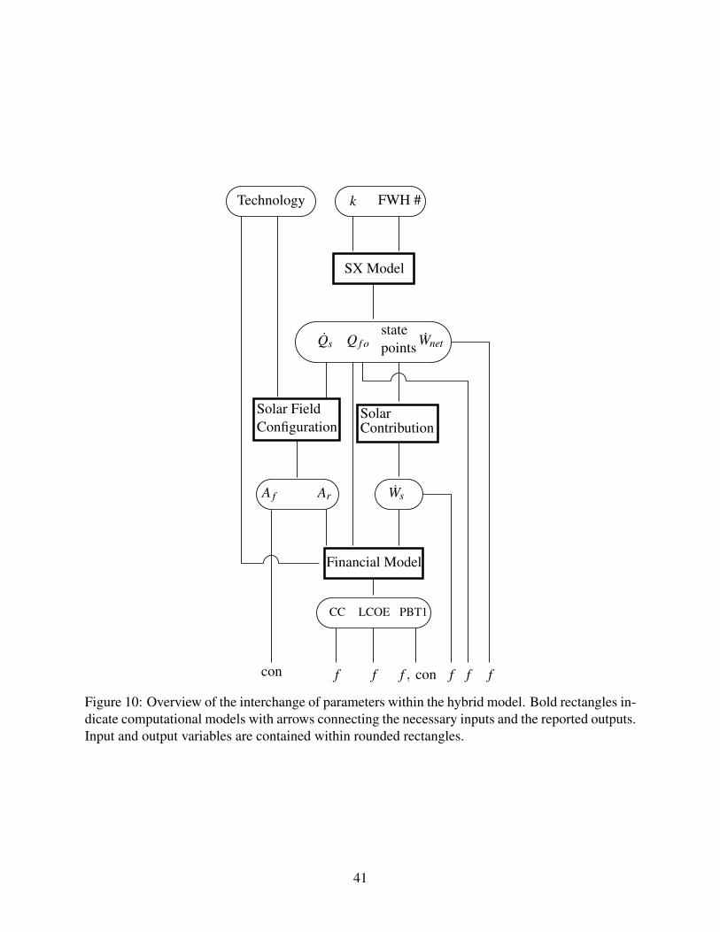
Technology FWH #k
SX Model
QsstatepointsQ f o Wnet
Solar FieldConfiguration
Ws
SolarContribution
Financial Model
ArA f
LCOE PBT1CC
f f f ff , concon f
Figure 10: Overview of the interchange of parameters within the hybrid model. Bold rectangles in-dicate computational models with arrows connecting the necessary inputs and the reported outputs.Input and output variables are contained within rounded rectangles.
41
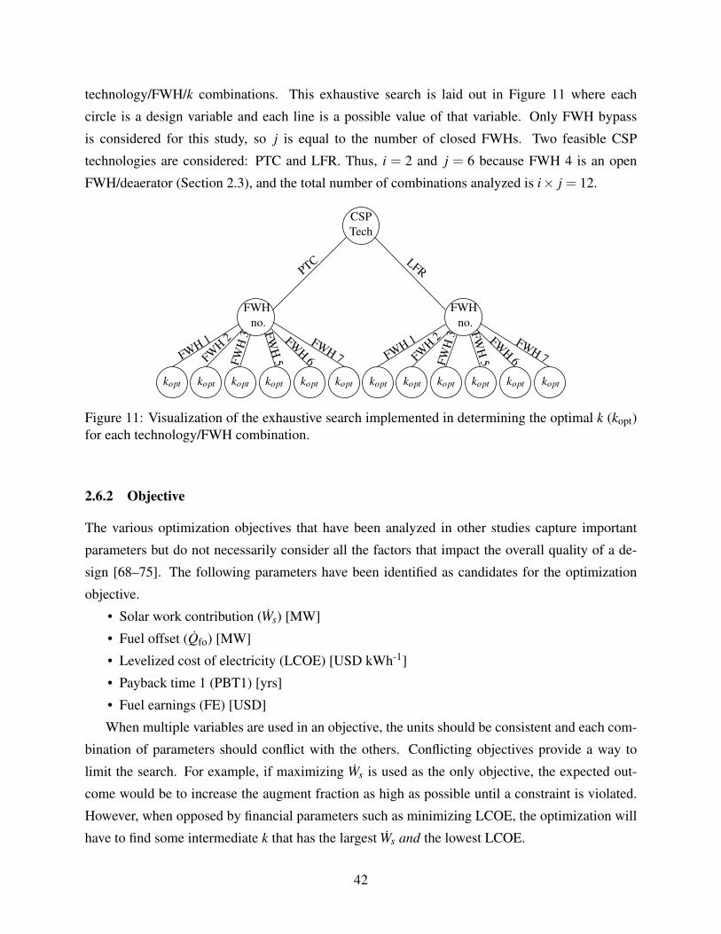
technology/FWH/k combinations. This exhaustive search is laid out in Figure 11 where each
circle is a design variable and each line is a possible value of that variable. Only FWH bypass
is considered for this study, so j is equal to the number of closed FWHs. Two feasible CSP
technologies are considered: PTC and LFR. Thus, i = 2 and j = 6 because FWH 4 is an open
FWH/deaerator (Section 2.3), and the total number of combinations analyzed is i× j = 12.
CSPTech
PTC LFR
FWHno.
FWH 1
FWH
2
FWH
3 FWH
5
FWH
6FWH 7 FWH 1
FWH
2
FWH
3 FWH
5
FWH
6FWH 7
koptkoptkoptkoptkoptkoptkoptkoptkoptkoptkoptkopt
FWHno.
Figure 11: Visualization of the exhaustive search implemented in determining the optimal k (kopt)for each technology/FWH combination.
2.6.2 Objective
The various optimization objectives that have been analyzed in other studies capture important
parameters but do not necessarily consider all the factors that impact the overall quality of a de-
sign [68–75]. The following parameters have been identified as candidates for the optimization
objective.
• Solar work contribution (Ws) [MW]
• Fuel offset (Qfo) [MW]
• Levelized cost of electricity (LCOE) [USD kWh-1]
• Payback time 1 (PBT1) [yrs]
• Fuel earnings (FE) [USD]
When multiple variables are used in an objective, the units should be consistent and each com-
bination of parameters should conflict with the others. Conflicting objectives provide a way to
limit the search. For example, if maximizing Ws is used as the only objective, the expected out-
come would be to increase the augment fraction as high as possible until a constraint is violated.
However, when opposed by financial parameters such as minimizing LCOE, the optimization will
have to find some intermediate k that has the largest Ws and the lowest LCOE.
42
The MATLAB function ‘fmincon’, included within the MATLAB optimization package, has
been selected to perform the continuous search for this study. Because ‘fmincon’ searches for the
minimum value of the specified objective, care must be given to combine the variables above such
that the ideal value will be a minimum. For best performance, multiple objectives should also have
consistent units and be of comparable orders of magnitude.
If the sub-objectives are of different orders of magnitude, one objective will dominate the
convergence criteria specified for the optimization termination. For example, if one sub-objective
has an initial value of 100 and a second sub-objective is 1, the total objective could be 101. The
next iteration in the optimization search may not result in any change in sub-objective 1, but a
100% increase in sub-objective 2. The total objective value would then be 102 with less than 1%
change. Thus, sub-objectives may require an additional constant multiple to achieve consistent
orders of magnitude.
Objective parameters are separated in two categories based on impact of plant thermodynamics
or economics. The total objective ( f ) can then be expressed in terms of the objective parameters
(Equation 22) where Ws and Qfo are scaled by the net work output by the plant (Wnet). The fi-
nancial parameters are combined to achieve dimensional homogeneity. To penalize Qfo < 0, the
optimization is set up such that each sub-objective would drive toward a maximum. Multiplying by
-1 effectively turns the maximization problem into a minimization problem, satisfying ‘fmincon’
minimum search preference. Each sub-objective will have units kW USD-1.
f ∝− Qfo Ws
CC Wnet− 1
LCOE (365 PBT1 hsun)(22)
Further control of sub-objective impact is achieved by applying weights (ω) to each sub-
objective. The weight for each sub-objective is determined by the developer, but the sum of all
weights should equal 1 (ω1+ω2+ · · · ωN = 1). As an example, for plants that have strict environ-
mental goals, increasing Qfo may be more important than financial outcomes, so this process can
be implemented with ω1 > ω2. Conversely, if financial performance is most important, ω2 > ω1
will provide the desired optimum.
f =−ω1Qfo Ws
CC Wnet107−ω2
1LCOE (365 PBT1 hsun)
102 (23)
Additional constants are multiplied with the objectives as necessary to reach comparable orders
of magnitude and dimensional homogeneity, such as converting PBT1 from years to hours by
multiplying 365 days/year and hsun.1 For best optimization results, the starting point given to
111.9 hr day-1 in Castle Dale
43

0 5 10 15
Augment Fraction (k) [%]
-50
0
50
100
150
200
250FWH 1
FWH 2
FWH 3
FWH 5
FWH 6
FWH 7
Figure 12: Behavior of Qfo. FWH 1 and FWH 2 bypass does not show a decrease in fuel consump-tion. Other bypass options only reduce fuel consumption once k > kFWH.
‘fmincon’ should be within the feasible design space.
The range of financially feasible designs can be approximated by analyzing the behavior of
Qfo with respect to k, as shown in Figure 12. All bypass options are negative for low k. Each
option seems to approach 0 at kFWH, or the k equivalent to the heating load of the bypassed FWH
at nominal operating conditions. Analyzing the state points of the solar integration model for each
of the LP integration options shows that the water boils at k > 3%. Considering kFWH ≈ 2−3% for
all LP integration options, no LP option is considered feasible for complete FWH bypass. Once
k > kFWH, the CSP field is starting to contribute more thermal energy and Qfo increases. One
option to expand the region of feasible designs based on Qfo is partial FWH bypass as opposed to
complete FWH bypass, the focus of this current work.
44

2.6.3 Constraints
Additional constraints were placed within the individual models used in the optimization to ensure
the outputs were feasible, such as confirming the components within the hybrid model simulation
met requirements for the conservation of energy. However, additional constraints are required to
ensure the designs generated in the optimization search are feasible for the desired application.
Two additional constraints have been applied restricting the size of the solar field and the du-
ration of PBT1. The optimization constrained the designs to limit the size of the solar field area
below a maximum size specified by the user. For this analysis, it is assumed there is an area of 20
ac (81,000 m2) available for a solar field.2 A second constraint specifies that the PBT1 be less than
the expected project lifetime specified by the user. A project life of 30 years is assumed for this
study.
2For Hunter, an area of approximately 45000 m2 (12 ac) has been identified as a candidate for CSP installation.
45
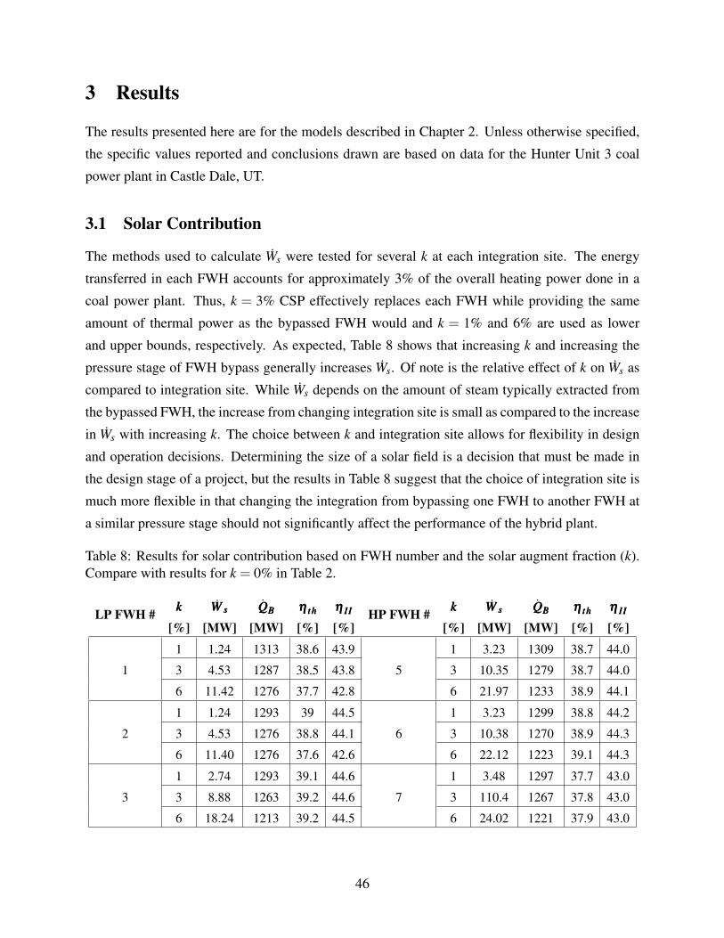
3 Results
The results presented here are for the models described in Chapter 2. Unless otherwise specified,
the specific values reported and conclusions drawn are based on data for the Hunter Unit 3 coal
power plant in Castle Dale, UT.
3.1 Solar Contribution
The methods used to calculate Ws were tested for several k at each integration site. The energy
transferred in each FWH accounts for approximately 3% of the overall heating power done in a
coal power plant. Thus, k = 3% CSP effectively replaces each FWH while providing the same
amount of thermal power as the bypassed FWH would and k = 1% and 6% are used as lower
and upper bounds, respectively. As expected, Table 8 shows that increasing k and increasing the
pressure stage of FWH bypass generally increases Ws. Of note is the relative effect of k on Ws as
compared to integration site. While Ws depends on the amount of steam typically extracted from
the bypassed FWH, the increase from changing integration site is small as compared to the increase
in Ws with increasing k. The choice between k and integration site allows for flexibility in design
and operation decisions. Determining the size of a solar field is a decision that must be made in
the design stage of a project, but the results in Table 8 suggest that the choice of integration site is
much more flexible in that changing the integration from bypassing one FWH to another FWH at
a similar pressure stage should not significantly affect the performance of the hybrid plant.
Table 8: Results for solar contribution based on FWH number and the solar augment fraction (k).Compare with results for k = 0% in Table 2.
LP FWH # kkk
[%]WWW sss
[MW]QQQBBB
[MW]ηηη ttthhh
[%]ηηη IIIIII
[%]HP FWH # kkk
[%]WWW sss
[MW]QQQBBB
[MW]ηηη ttthhh
[%]ηηη IIIIII
[%]
1 1.24 1313 38.6 43.9 1 3.23 1309 38.7 44.0
1 3 4.53 1287 38.5 43.8 5 3 10.35 1279 38.7 44.0
6 11.42 1276 37.7 42.8 6 21.97 1233 38.9 44.1
1 1.24 1293 39 44.5 1 3.23 1299 38.8 44.2
2 3 4.53 1276 38.8 44.1 6 3 10.38 1270 38.9 44.3
6 11.40 1276 37.6 42.6 6 22.12 1223 39.1 44.3
1 2.74 1293 39.1 44.6 1 3.48 1297 37.7 43.0
3 3 8.88 1263 39.2 44.6 7 3 110.4 1267 37.8 43.0
6 18.24 1213 39.2 44.5 6 24.02 1221 37.9 43.0
46
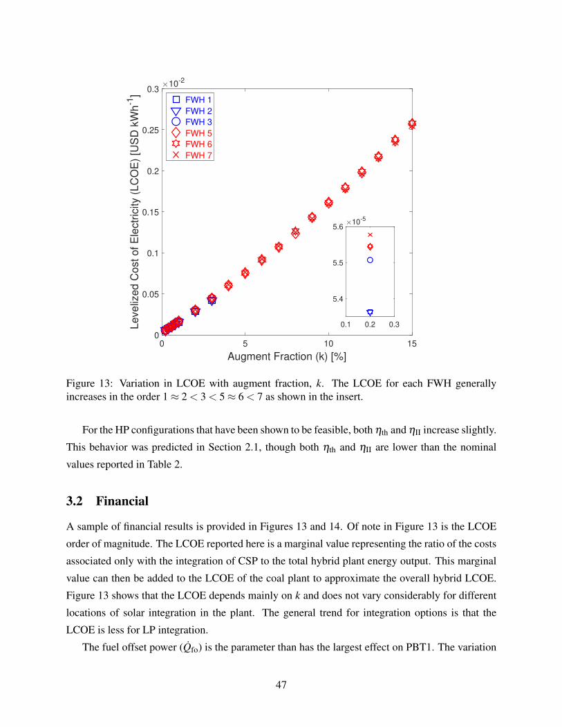
0 5 10 15
Augment Fraction (k) [%]
0
0.05
0.1
0.15
0.2
0.25
0.3
Le
ve
lize
d C
ost
of
Ele
ctr
icity (
LC
OE
) [U
SD
kW
h-1
]
10-2
FWH 1
FWH 2
FWH 3
FWH 5
FWH 6
FWH 7
0.1 0.2 0.3
5.4
5.5
5.610
-5
Figure 13: Variation in LCOE with augment fraction, k. The LCOE for each FWH generallyincreases in the order 1≈ 2 < 3 < 5≈ 6 < 7 as shown in the insert.
For the HP configurations that have been shown to be feasible, both ηth and ηII increase slightly.
This behavior was predicted in Section 2.1, though both ηth and ηII are lower than the nominal
values reported in Table 2.
3.2 Financial
A sample of financial results is provided in Figures 13 and 14. Of note in Figure 13 is the LCOE
order of magnitude. The LCOE reported here is a marginal value representing the ratio of the costs
associated only with the integration of CSP to the total hybrid plant energy output. This marginal
value can then be added to the LCOE of the coal plant to approximate the overall hybrid LCOE.
Figure 13 shows that the LCOE depends mainly on k and does not vary considerably for different
locations of solar integration in the plant. The general trend for integration options is that the
LCOE is less for LP integration.
The fuel offset power (Qfo) is the parameter than has the largest effect on PBT1. The variation
47
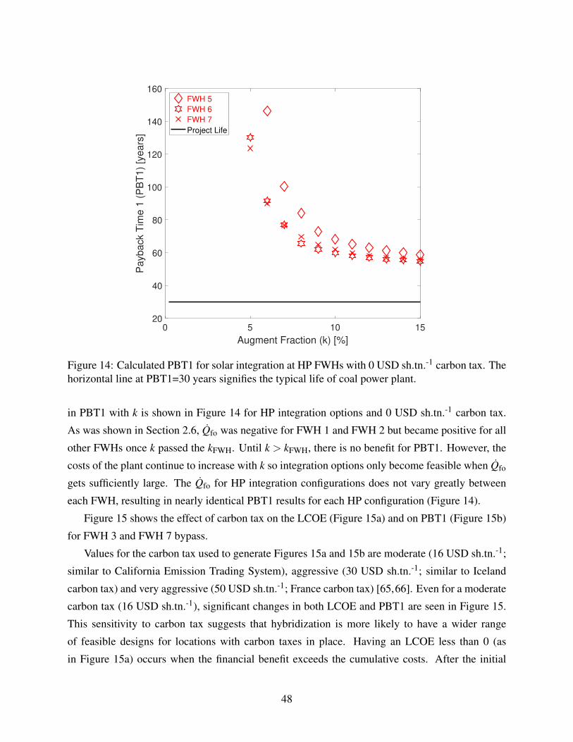
0 5 10 15
Augment Fraction (k) [%]
20
40
60
80
100
120
140
160
Payback T
ime 1
(P
BT
1)
[years
]
FWH 5
FWH 6
FWH 7
Project Life
Figure 14: Calculated PBT1 for solar integration at HP FWHs with 0 USD sh.tn.-1 carbon tax. Thehorizontal line at PBT1=30 years signifies the typical life of coal power plant.
in PBT1 with k is shown in Figure 14 for HP integration options and 0 USD sh.tn.-1 carbon tax.
As was shown in Section 2.6, Qfo was negative for FWH 1 and FWH 2 but became positive for all
other FWHs once k passed the kFWH. Until k > kFWH, there is no benefit for PBT1. However, the
costs of the plant continue to increase with k so integration options only become feasible when Qfo
gets sufficiently large. The Qfo for HP integration configurations does not vary greatly between
each FWH, resulting in nearly identical PBT1 results for each HP configuration (Figure 14).
Figure 15 shows the effect of carbon tax on the LCOE (Figure 15a) and on PBT1 (Figure 15b)
for FWH 3 and FWH 7 bypass.
Values for the carbon tax used to generate Figures 15a and 15b are moderate (16 USD sh.tn.-1;
similar to California Emission Trading System), aggressive (30 USD sh.tn.-1; similar to Iceland
carbon tax) and very aggressive (50 USD sh.tn.-1; France carbon tax) [65,66]. Even for a moderate
carbon tax (16 USD sh.tn.-1), significant changes in both LCOE and PBT1 are seen in Figure 15.
This sensitivity to carbon tax suggests that hybridization is more likely to have a wider range
of feasible designs for locations with carbon taxes in place. Having an LCOE less than 0 (as
in Figure 15a) occurs when the financial benefit exceeds the cumulative costs. After the initial
48
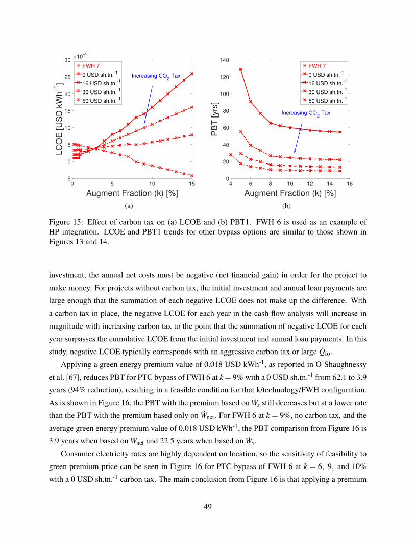
0 5 10 15
Augment Fraction (k) [%]
-5
0
5
10
15
20
25
30L
CO
E [
US
D k
Wh
-1]
10-4
FWH 7
0 USD sh.tn.-1
16 USD sh.tn.-1
30 USD sh.tn.-1
50 USD sh.tn.-1
Increasing CO2 Tax
(a)
4 6 8 10 12 14 16
Augment Fraction (k) [%]
0
20
40
60
80
100
120
140
PB
T [
yrs
]
FWH 7
0 USD sh.tn.-1
16 USD sh.tn.-1
30 USD sh.tn.-1
50 USD sh.tn.-1
Increasing CO2 Tax
(b)
Figure 15: Effect of carbon tax on (a) LCOE and (b) PBT1. FWH 6 is used as an example ofHP integration. LCOE and PBT1 trends for other bypass options are similar to those shown inFigures 13 and 14.
investment, the annual net costs must be negative (net financial gain) in order for the project to
make money. For projects without carbon tax, the initial investment and annual loan payments are
large enough that the summation of each negative LCOE does not make up the difference. With
a carbon tax in place, the negative LCOE for each year in the cash flow analysis will increase in
magnitude with increasing carbon tax to the point that the summation of negative LCOE for each
year surpasses the cumulative LCOE from the initial investment and annual loan payments. In this
study, negative LCOE typically corresponds with an aggressive carbon tax or large Qfo.
Applying a green energy premium value of 0.018 USD kWh-1, as reported in O’Shaughnessy
et al. [67], reduces PBT for PTC bypass of FWH 6 at k = 9% with a 0 USD sh.tn.-1 from 62.1 to 3.9
years (94% reduction), resulting in a feasible condition for that k/technology/FWH configuration.
As is shown in Figure 16, the PBT with the premium based on Ws still decreases but at a lower rate
than the PBT with the premium based only on Wnet. For FWH 6 at k = 9%, no carbon tax, and the
average green energy premium value of 0.018 USD kWh-1, the PBT comparison from Figure 16 is
3.9 years when based on Wnet and 22.5 years when based on Ws.
Consumer electricity rates are highly dependent on location, so the sensitivity of feasibility to
green premium price can be seen in Figure 16 for PTC bypass of FWH 6 at k = 6, 9, and 10%
with a 0 USD sh.tn.-1 carbon tax. The main conclusion from Figure 16 is that applying a premium
49

considerably decreases PBT with all else constant. However, there is a limit at which increasing
the premium price no longer shows significant decreases in PBT. For Figure 16, the change in PBT
is less than 2% when it is increased beyond 0.0155 USD kWh-1. The premium of 0.0155 USD
kWh-1 is sufficient to reduce PBT to 4.3 years for k = 9%.
0 0.005 0.01 0.015 0.02
Green Energy Premium Cost [USD kWh-1
]
0
20
40
60
80
100
PB
T [years
]
Solar Contribution Premium
Total Power Premium
k=6%
k=9%
k=10%
Figure 16: Effect of green premium price and k on PBT1.
Looking at the effect of a carbon tax (Figure 15b) and a green premium electricity price (Fig-
ure 16) show similar trends in the effect on PBT from carbon tax and green premium. Increasing a
carbon tax or green premium will decrease the PBT, but adjusting the green premium has a greater
impact than increasing the carbon tax. This is due to how each value is implemented in this study,
as discussed in Section ??. A carbon tax is applied to the coal saved by solar augmentation, typ-
ically as high as 100 MW for low-solar augmentation. The green premium, however, is applied
to all the electricity generated during hsun throughout the year. For the Hunter Unit 3 plant with
a nameplate generation of almost 500 MWe, the green premium is effectively applied to a greater
source of power.
50
3.3 Optimization
As described in Section 2.6, hybrid performance is divided in thermodynamic and economic cat-
egories. Figure 17 shows the relationship between the two objectives for weights in increments
of ω = 0.2 (i.e. ω1 = [0, 0.2, 0.4, · · · , 1], and ω2 = [1, 0.8, 0.6, · · · , 0]) for HP FWHs and 16
USD sh.tn.-1 carbon tax. The curves represented by the trendlines fit to the calculated optimums
are Pareto fronts. The Pareto front for two-objective optimization is a curve that represents the
hypothetical boundary for feasible designs. In the case of this study, the optimization objective
was written such that the optimal design would trend towards the minimum of each objective. In
Figure 17, the Pareto fronts suggest that the majority of other feasible designs result in a higher
value for at least one of the two objectives.
As expected, the trendline reflects an inverse relationship and the objectives contradict each
other. The trendline fit to the sample simulations demonstrates the expected pareto front of feasible
designs for different possible ω combinations. The results in Figure 17 result in the majority of
the ω combinations lying closer toward a thermodynamic minimum, suggesting that OBJ1 may
be dominating the optimization. In general, the trendline representing the Pareto front for FWH
6 bypass lies below all other designs, suggesting FWH 6 bypass is most likely to be the optimal
integration site for a hybrid plant when compared to results for each of the other FWHs.
Results from Section 3.2 show that k, directly tied to the capital cost, has the largest impact on
financial performance and overall feasibility of a hybrid project once Qfo > 0 (Figure 13). Thus,
more weight is given to the financial objective, or ω1 = 0.2, ω2 = 0.8. Optimization results for
each FWH and Technology type are given in Table 9 assuming a project life of 30 years and a
maximum allowable solar field of 30 ac. As shown in Figure 11, kopt is found for each FWH
bypass option combined with either PTC or LFR for the solar field.
The optimization results in Table 9 show the kopt for each technology/FWH combination. The
overall hybrid optimal design is found by selecting the configuration resulting in the lowest (most
negative) value for f (Section 2.6). For this study, k = 9% PTC bypassing FWH 6 is the optimal
configuration for 16 USD sh.tn.-1 carbon tax. This result is consistent with similar work published
in archival literature suggesting hybrid performance improves as the integration site approaches
the boiler stage [40, 76]. It was expected that LFR integration would be generally less feasible
than PTC due to higher capital costs. This is evident in that none of the optimal designs for LFR
had feasible PBT1. However, the efficiency of LFR land use is apparent throughout Table 9, but
particularly for FWH 5 bypass where the estimated solar field for the LFR configuration is similar
to the PTC configuration despite a higher kopt than PTC FWH 5 bypass [77].
51
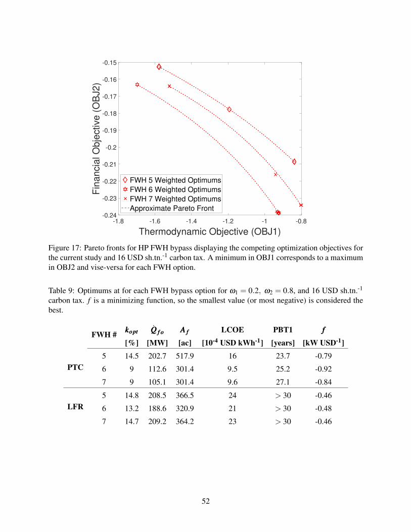
-1.8 -1.6 -1.4 -1.2 -1 -0.8
Thermodynamic Objective (OBJ1)
-0.24
-0.23
-0.22
-0.21
-0.2
-0.19
-0.18
-0.17
-0.16
-0.15
Fin
an
cia
l O
bje
ctive
(O
BJ2
)
FWH 5 Weighted Optimums
FWH 6 Weighted Optimums
FWH 7 Weighted Optimums
Approximate Pareto Front
Figure 17: Pareto fronts for HP FWH bypass displaying the competing optimization objectives forthe current study and 16 USD sh.tn.-1 carbon tax. A minimum in OBJ1 corresponds to a maximumin OBJ2 and vise-versa for each FWH option.
Table 9: Optimums at for each FWH bypass option for ω1 = 0.2, ω2 = 0.8, and 16 USD sh.tn.-1
carbon tax. f is a minimizing function, so the smallest value (or most negative) is considered thebest.
FWH # kkkooopppttt
[%]
QQQ fff ooo
[MW]
AAA fff
[ac]LCOE
[10-4 USD kWh-1]PBT1[years]
fff
[kW USD-1]
PTC5 14.5 202.7 517.9 16 23.7 -0.79
6 9 112.6 301.4 9.5 25.2 -0.92
7 9 105.1 301.4 9.6 27.1 -0.84
LFR5 14.8 208.5 366.5 24 > 30 -0.46
6 13.2 188.6 320.9 21 > 30 -0.48
7 14.7 209.2 364.2 23 > 30 -0.46
52
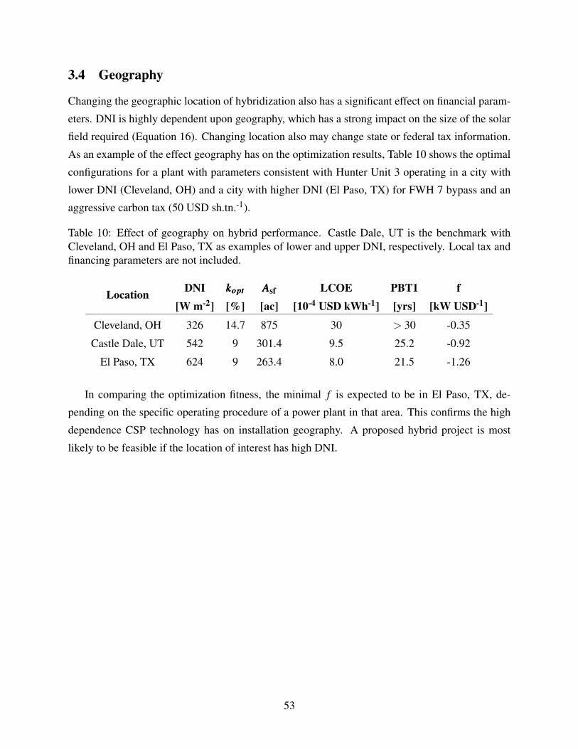
3.4 Geography
Changing the geographic location of hybridization also has a significant effect on financial param-
eters. DNI is highly dependent upon geography, which has a strong impact on the size of the solar
field required (Equation 16). Changing location also may change state or federal tax information.
As an example of the effect geography has on the optimization results, Table 10 shows the optimal
configurations for a plant with parameters consistent with Hunter Unit 3 operating in a city with
lower DNI (Cleveland, OH) and a city with higher DNI (El Paso, TX) for FWH 7 bypass and an
aggressive carbon tax (50 USD sh.tn.-1).
Table 10: Effect of geography on hybrid performance. Castle Dale, UT is the benchmark withCleveland, OH and El Paso, TX as examples of lower and upper DNI, respectively. Local tax andfinancing parameters are not included.
Location DNI[W m-2]
kkkooopppttt
[%]AAAsf
[ac]LCOE
[10-4 USD kWh-1]PBT1[yrs]
f[kW USD-1]
Cleveland, OH 326 14.7 875 30 > 30 -0.35
Castle Dale, UT 542 9 301.4 9.5 25.2 -0.92
El Paso, TX 624 9 263.4 8.0 21.5 -1.26
In comparing the optimization fitness, the minimal f is expected to be in El Paso, TX, de-
pending on the specific operating procedure of a power plant in that area. This confirms the high
dependence CSP technology has on installation geography. A proposed hybrid project is most
likely to be feasible if the location of interest has high DNI.
53

4 Conclusion
The data presented shows that the integration site in the power plant causes the greatest effect on
plant performance; k and CSP technology type have the greatest impact on financial performance.
Hybridization has an impact beyond just plant efficiency and LCOE.
The US Energy Information Administration reports that the amount of CO2 emissions from a
coal power plant can be estimated by the conversion factor 205 lb. CO2 MMBTU-1 for bituminous
coal [12]. With FWH 6 bypass as an example, Table 9 shows that 52 MW worth of coal is offset
during hybrid mode. Using the effective solar time to convert from MW to MMBTU and projecting
throughout the year, the conversion from the Energy Information Administration results in a CO2
emissions reduction of approximately 171 tons per year. According to Bernal et al. [78], a typical
temperate, dry conifer forest (the most prominent forest in UT) removes approximately 6.4 t CO2
ha-1 year-1. Thus, CSP augmentation in UT reduces emissions equivalent to approximately 27,000
ha of dry conifer forest for k = 9% PTC augmentation at FWH 6 bypass.
This study analyzes a retrofit hybrid model operating in fuel saving mode, but Manente showed
that plants constructed with hybrid capabilities, typically operating in power boost mode, can also
see considerable benefits [23]. Manente’s study, focused on integrated solar combined cycles,
shows that the inclusion of solar in the power generation process can add 50 MWe to an exist-
ing plant without changing any equipment. Included in Manente’s study was the requirement to
upgrade the turbine to account for the potential increase in capacity. This suggests that a power
boost analysis is best for initial construction and plants anticipating upgrades to turbines or electri-
cal transformers due to the added capital cost of higher capacity components whereas fuel saving
mode is best for retrofit projects.
The impact of hybridization can be extended with the addition of thermal energy storage (TES).
Storage technology has been studied for use in building energy efficiency [79] as well as CSP.
Common options for storage materials include phase change materials [80,81], large collections of
rock [82], and molten salts [83]. Studies show that TES can add considerably to the hybridization
benefit [84–87]. The inclusion of TES would cause changes in the financial performance of a
hybrid plant necessitating edits to the model presented in the current study. The operation of the
plant would largely be the same with the exception that the hybrid plant would be able to operate
in fuel saving mode for a longer period of time. This increase in effective solar time is expected
to increase the total amount of coal saved over time and cause a potential decrease in LCOE and
PBT1 depending on the selection of TES technology.
While benefits of hybrid technology have been explored in published literature, this study has
contributed a simplified method to evaluate preliminary hybridization feasibility based on a repre-
54

sentative coal power plant. The representative model was shown to be applicable to Hunter Unit 3
in Castle Dale, UT and a separate coal power plant with a different configuration [28]. Using solar
data from NREL and standard equipment dimensions, the solar resource for the hybrid geography
was quantified and combined with the representative model in the solar integration model. The
fraction of power out of the hybrid power plant that can be attributed to the solar integration was
calculated using an exergy analysis. A financial model was used to calculate comparative parame-
ters including LCOE, PBT1, and fuel earnings. The performance of the solar heat exchange model
is combined with the financial performance to define the optimization objective used to find the op-
timal configuration for a proposed hybrid retrofit project. Results from simulating CSP integration
into Hunter Unit 3 suggest that hybridization may be feasible considering the expected thermody-
namic benefits to the power plant and the LCOE and PBT1 for small k. LFR requires less land
for a solar field than PTC, but higher capital costs universally preclude the use of LFR in hybrid
projects according to the assumptions of this analysis. As expected, areas with higher average DNI
are more promising candidates for Ws and areas with lower DNI are less feasibile. It is shown that
for a possible scenario including a carbon tax, the LCOE and PBT1 will decrease accordingly and
increase the feasibility of hybridization. The impact of a green premium on consumer electricity
prices is also demonstrated to have a dramatic effect on decreasing PBT1. Carbon taxes and green
premium prices are common in communities across the world [65, 67], so a combination of both
incentives makes CSP-coal hybridization feasible and competitive with other power generation op-
tions. The method presented in this paper, while simplified, is largely irrespective of any particular
coal plant, geography, or local tax code. The results suggest a generous range of feasible hybrid
configurations, but do not provide an explicit commentary on public policy. While the effects of
carbon tax on feasibility as defined in this analysis are substantial, there are many and various
effects of carbon tax on an economy and social structure such that this study alone cannot be used
to argue for or against the implementation of a carbon tax or other applicable policies. Instead, it
is only suggested that hybridization be considered where such policies may be in place.
55
References
[1] U.S. Energy Information Administration, 2020. Annual Energy Review
https://www.eia.gov/totalenergy/data/annual/ (Accessed on 07 Jan 2021).
[2] Keho, Y., 2016. “What drives energy consumption in developing countries? The
experience of selected African countries.” Energy Policy, 91, 4, pp. 233–246.
[3] U.S. Energy Information Administration, 2016. Carbon Dioxide Emissions Coefficients by
Fuel.
[4] Kostic, M. M., 2015. “Energy: Global and historical background.” Encyclopedia of Energy
Engineering, 06, p. 15.
[5] Stevens, L., Anderson, B., Cowan, C., Colton, K., and Johnson, D., 2017. The Footprint of
Energy: Land Use of U.S. Electricity Production Tech. rep., Strata, 6.
[6] National Renewable Energy Laboratory, 2020. Annual Technology Baseline
https://atb.nrel.gov/electricity/2020/ (Accessed on 09 Oct. 2020.
[7] Zhang, H. L., Baeyens, J., Degreve, J., and Caceres, G., 2013. “Concentrated solar power
plants: Review and design methodology.” Renewable and Sustainable Energy Reviews, 22,
pp. 466–481.
[8] Zoschak, R., and Wu, S., 1975. “Studies of the direct input of solar energy to a
fossil-fueled central station steam power plant.” Solar Energy, 17(5), 11, pp. 297–305.
[9] De Laquil III, P., Kearney, D., Geyer, M., and Diver, R., 1993. “Solar-Thermal Electric
Technology.” In Renewable Energy: Sources for Fuels and Electricity, T. B. Johansson,
H. Kelly, A. K. N. Reddy, and R. H. Williams, eds. Island Press, Washington, D.C., ch. 5,
pp. 234–6.
[10] Turchi, C., Langle, N., Bedilion, R., and Libby, C., 2011. Solar-Augment Potential of U.S.
Fossil-Fired Power Plants Tech. rep., National Renewable Energy Laboratory, Golden, CO.
[11] Pramanik, S., and Ravikrishna, R. V., 2017. “A review of concentrated solar power hybrid
technologies.” Applied Thermal Engineering, 127, pp. 602–637.
[12] U.S. Energy Information Administration, 2016. Carbon Dioxide Emissions Coefficients by
Fuel https://www.eia.gov/environment/emissions/co2 vol mass.php (Accessed on 14 Apr.
2020).
56
[13] New York Times, 1916. American Inventor Uses Egypt’s Sun for Power, 7.
[14] Kalogirou, S., 2007. “Recent Patents in Solar Energy Collectors and Applications.” Recent
Patents on Engineering, 1(1), 2, pp. 23–33.
[15] Peterseim, J. H., White, S., Tadros, A., and Hellwig, U., 2013. “Concentrated solar power
hybrid plants, which technologies are best suited for hybridisation?.” Renewable Energy,
57, pp. 520–532.
[16] Libby, C., Meagher, P., and Cerezo, L., 2010. Solar-Fossil Hybrid Power Plants: Summary
Report on Conceptual Designs, 1022418 Tech. rep., Electric Power Research Institute,
Palo Alto, CA.
[17] Powell, K. M., Rashid, K., Ellingwood, K., Tuttle, J., and Iverson, B. D., 2017. “Hybrid
concentrated solar thermal power systems: A review.” Renewable and Sustainable Energy
Reviews, 80, pp. 215–237.
[18] Li, Y., and Yang, Y., 2014. “Thermodynamic analysis of a novel integrated solar combined
cycle.” Applied Energy, 122, pp. 133–142.
[19] Zhao, Y., Liu, M., Wang, C., Li, X., Chong, D., and Yan, J., 2018. “Increasing operational
flexibility of supercritical coal-fired power plants by regulating thermal system
configuration during transient processes.” Applied Energy, 228(July), pp. 2375–2386.
[20] Mohammadi, K., Khanmohammadi, S., Khorasanizadeh, H., and Powell, K., 2020. “A
comprehensive review of solar only and hybrid solar driven multigeneration systems:
Classifications, benefits, design and prospective.” Applied Energy, 268(March).
[21] Ihsan, A., Jeppesen, M., and Brear, M. J., 2019. “Impact of demand response on the
optimal, techno-economic performance of a hybrid, renewable energy power plant.”
Applied Energy, 238(January), pp. 972–984.
[22] Zhai, R., Li, C., Chen, Y., Yang, Y., Patchigolla, K., and Oakey, J. E., 2016. “Life cycle
assessment of solar aided coal-fired power system with and without heat storage.” Energy
Conversion and Management, 111, pp. 453–465.
[23] Manente, G., 2016. “High performance integrated solar combined cycles with minimum
modifications to the combined cycle power plant design.” Energy Conversion and
Management, 111, pp. 186–197.
57
[24] Behar, O., Khellaf, A., Mohammedi, K., and Ait-Kaci, S., 2014. “A review of integrated
solar combined cycle system (ISCCS) with a parabolic trough technology.” Renewable and
Sustainable Energy Reviews, 39, 7, pp. 223–250.
[25] Rech, S., Lazzaretto, A., and Grigolon, E., 2018. “Optimum integration of concentrating
solar technologies in a real coal-fired power plant for fuel saving.” Energy Conversion and
Management, 178(October), pp. 299–310.
[26] Peng, S., Wang, Z., Hong, H., Xu, D., and Jin, H., 2014. “Exergy evaluation of a typical
330 MW solar-hybrid coal-fired power plant in China.” Energy Conversion and
Management, 85, pp. 848–855.
[27] Zhao, Y., Hong, H., and Jin, H., 2017. “Optimization of the solar field size for the
solar–coal hybrid system.” Applied Energy, 185, pp. 1162–1172.
[28] Adibhatla, S., and Kaushik, S. C., 2017. “Energy, exergy, economic and environmental
(4E) analyses of a conceptual solar aided coal fired 500 MWe thermal power plant with
thermal energy storage option.” Sustainable Energy Technologies and Assessments, 21,
pp. 89–99.
[29] Okoroigwe, E., and Madhlopa, A., 2016. “An integrated combined cycle system driven by
a solar tower: A review.” Renewable and Sustainable Energy Reviews, 57, pp. 337–350.
[30] Binamer, A. O., 2019. “Al-Abdaliya integrated solar combined cycle power plant: Case
study of Kuwait, part I.” Renewable Energy, 131, 2, pp. 923–937.
[31] Sheu, E. J., Mitsos, A., Eter, A. A., Mokheimer, E. M. A., Habib, M. A., and Al-Qutub, A.,
2012. “A Review of Hybrid Solar–Fossil Fuel Power Generation Systems and Performance
Metrics.” Journal of Solar Energy Engineering, 134(4), p. 041006.
[32] Sinha, M., 2017. NTPC’s Dadri unit set to install solar-thermal hybrid power plant
https://energy.economictimes.indiatimes.com/news/renewable/ntpc-dadri-set-to-install-
solar-thermal-hybrid-plant/57804545 (Accessed on 12 Jun.
2020).
[33] National Renewable Energy Laboratory, 2020. Concentrating Solar Power Projects
https://solarpaces.nrel.gov/ (Accessed on 19 Nov. 2020).
58
[34] Madler, M., 2017. Regulators Approve Palmdale Power Plant
https://sfvbj.com/news/2017/aug/11/regulators-approve-palmdale-power-plant/ (Accessed
on 23 Apr. 2019).
[35] Johnson, S., 2018. Plug pulled on Victorville power plant as land lease pursued
https://www.vvdailypress.com/news/20180425/plug-pulled-on-victorville-power-plant-as-
land-lease-pursued (Accessed on 23 Apr.
2019).
[36] New Energy Update, 2017. CSP Today Global Tracker
http://tracker.newenergyupdate.com/tracker/projects (Accessed on 12 Jun. 2020).
[37] Alqahtani, B. J., and Patino-Echeverri, D., 2016. “Integrated Solar Combined Cycle Power
Plants: Paving the way for thermal solar.” Applied Energy, 169.
[38] Abdelhafidi, N., Bachari, N. E. I., Abdelhafidi, Z., Cheknane, A., Mokhnache, A., and
Castro, L., 2019. “Modeling of integrated solar combined cycle power plant (ISCC) of
Hassi R’mel, Algeria.” International Journal of Energy Sector Management, 14(3), p. 22.
[39] Tannous, C., Ahlam, D., and Rosa, M., 2016. “Renewable energy integration into existing
plants: Application: Deir Ammar thermal plant-North Lebanon.” In 2016 3rd International
Conference on Renewable Energies for Developing Countries, REDEC 2016, Institute of
Electrical and Electronics Engineers Inc., p. 9.
[40] Wang, F., Li, H., Zhao, J., Deng, S., and Yan, J., 2016. “Technical and economic analysis
of integrating low-medium temperature solar energy into power plant.” Energy Conversion
and Management, 112, pp. 459–469.
[41] Bakos, G. C., and Tsechelidou, C., 2013. “Solar aided power generation of a 300MW
lignite fired power plant combined with line-focus parabolic trough collectors field.”
Renewable Energy, 60, pp. 540–547.
[42] Zhao, Y., Hong, H., and Jin, H., 2015. “Thermo-economic Optimization of Solar-Coal
Hybrid Systems.” Energy Procedia, 75, pp. 457–461.
[43] Mokheimer, E. M., Dabwan, Y. N., and Habib, M. A., 2017. “Optimal integration of solar
energy with fossil fuel gas turbine cogeneration plants using three different CSP
technologies in Saudi Arabia.” Applied Energy, 185, pp. 1268–1280.
59

[44] Choudhary, T., and Sanjay, 2017. “Thermodynamic assessment of SOFC-ICGT hybrid
cycle: Energy analysis and entropy generation minimization.” Energy.
[45] Cengel, Y. A., and Boles, M. A., 2011. Thermodynamics: An Engineering Approach., 7 ed.
McGraw-Hill, New York, NY.
[46] National Renewable Energy Laboratory, 2018. National Solar Radiation Database
https://maps.nrel.gov/nsrdb-viewer (Accessed on 6 Nov. 2019).
[47] Sengupta, M., Xie, Y., Lopez, A., Habte, A., Maclaurin, G., and Shelby, J., 2018. “The
National Solar Radiation Data Base (NSRDB).” Renewable and Sustainable Energy
Reviews, 89, 6, pp. 51–60.
[48] Sait, H. H., Martinez-Val, J. M., Abbas, R., and Munoz-Anton, J., 2015. “Fresnel-based
modular solar fields for performance/cost optimization in solar thermal power plants: A
comparison with parabolic trough collectors.” Applied Energy, 141, 3, pp. 175–189.
[49] Rovira, A., Barbero, R., Montes, M. J., Abbas, R., and Varela, F., 2016. “Analysis and
comparison of Integrated Solar Combined Cycles using parabolic troughs and linear
Fresnel reflectors as concentrating systems.” Applied Energy.
[50] Moya, E. Z., 2012. “7 - Parabolic-trough concentrating solar power (CSP) systems.” In
Woodhead Publishing Series in Energy, K. Lovegrove and W. B. T. C. S. P. T. Stein, eds.
Woodhead Publishing, pp. 197–239.
[51] Zavoico, A. B., 2001. Solar Power Tower - Design Basis Document Tech. Rep.
SAND2001-2100, Sandia National Laboratories, San Francisco, CA.
[52] Lemmon, E. W., , Bell, I. H., Huber, M. L., and McLinden, M. O., 2018. NIST Standard
Reference Database 23: Reference Fluid Thermodynamic and Transport
Properties-REFPROP, Version 10.0, National Institute of Standards and Technology
https://www.nist.gov/srd/refprop (Accessed on 8 Jun. 2020).
[53] Eastman Chemical Company, 2019. THERMINOL VP-1 heat transfer fluid brochure
https://www.therminol.com/product/71093459?pn=Therminol-VP-1-Heat-Transfer-
Fluid (Accesed on 8 Jun.
2020).
60

[54] Qiu, Y., He, Y. L., Cheng, Z. D., and Wang, K., 2015. “Study on optical and thermal
performance of a linear Fresnel solar reflector using molten salt as HTF with MCRT and
FVM methods.” Applied Energy, 146, pp. 162–173.
[55] Vignarooban, K., Xu, X., Arvay, A., Hsu, K., and Kannan, A. M., 2015. “Heat transfer
fluids for concentrating solar power systems - A review.” Applied Energy, 146,
pp. 383–396.
[56] Channiwala, S. A., and Ekbote, A., 2015. “A Generalized Model to Estimate Field Size for
Solar-Only Parabolic Trough Plant.” Third South African Solar Energy Conference,
3(May), pp. 283–288.
[57] Hou, H., Xu, Z., and Yang, Y., 2016. “An evaluation method of solar contribution in a solar
aided power generation (SAPG) system based on exergy analysis.” Applied Energy, 182,
pp. 1–8.
[58] Freeman, J., Blair, N., Guittet, D., Boyd, M., Neises, T., Wagner, M., Janzou, S., and
Gilman, P., 2018. System Advisor Model.
[59] GmbH, B.-D., Band, D., and Michalzik, R., 2009. BUDGET OFFER REVISION 3 Solar
Steam Generator System PROJECT: SOLANA Tech. rep., SPX, Ratingen.
[60] Montes, M. J., Rovira, A., Munoz, M., and Martınez-Val, J. M., 2011. “Performance
analysis of an Integrated Solar Combined Cycle using Direct Steam Generation in
parabolic trough collectors.” Applied Energy, 88, pp. 3228–3238.
[61] Turchi, C., 2010. Parabolic Trough Reference Plant for Cost Modeling with the Solar
Advisor Model ( SAM ) Tech. Rep. July, National Renewable Energy Laboratory, Golden,
CO.
[62] Tax-Rates, 2020. Utah Property Taxes 2020 http://www.tax-rates.org/ (Accessed on 25
Jan. 2020).
[63] Bailey, N., 2019. Interview With Nathan Bailey from PacifiCorp.
[64] Energysage, 2020. Investment tax credit for solar power
https://www.energysage.com/solar/cost-benefit/solar-investment-tax-credit/ (Accessed on
24 Jan. 2020).
61
[65] Ramstein, C., Dominioni, G., Ettehad, S., Lam, L., Quant, M., Zhang, J., Mark, L., Nierop,
S., Berg, T., Leuschner, P., Merusi, C., Klein, N., and Trim, I., 2019. State and Trends of
Carbon Pricing 2019 Tech. Rep. June 2019, World Bank Group, Washington, D.C.
[66] PacifiCorp IRP Resource Planning, 2019. 2019 Integrated Resource Plan Tech. rep.,
PacifiCorp, Portland, OR.
[67] O’Shaughnessy, E., Heeter, J., Cook, J., and Volpi, C., 2017. Status and Trends in the US
Voluntary Green Power Market (2016 Data) Tech. Rep. TP-6A20-70174, National
Renewable Energy Laboratory, Golden, CO.
[68] Zhai, R., Zhao, M., Tan, K., and Yang, Y., 2015. “Optimizing operation of a solar-aided
coal-fired power system based on the solar contribution evaluation method.” Applied
Energy, 146, 5, pp. 328–334.
[69] Wang, Y., Xu, J., Chen, Z., Cao, H., and Zhang, B., 2017. “Technical and economical
optimization for a typical solar hybrid coal-fired power plant in China.” Applied Thermal
Engineering, 115, pp. 549–557.
[70] Quirante, N., Caballero, J. A., and Grossmann, I. E., 2017. “A novel disjunctive model for
the simultaneous optimization and heat integration.” Computers & Chemical Engineering,
96, 1, pp. 149–168.
[71] Donado, K., Navarro, L., Quintero, M. C. G., and Pardo, M., 2019. “HYRES: A
multi-objective optimization tool for proper configuration of renewable hybrid energy
systems.” Energies, 13(1), 12.
[72] Wang, J., Duan, L., Yang, Y., Yang, Z., and Yang, L., 2019. “Study on the general system
integration optimization method of the solar aided coal-fired power generation system.”
Energy, 2, pp. 660–673.
[73] Baghernejad, A., and Yaghoubi, M., 2011. “Exergoeconomic analysis and optimization of
an Integrated Solar Combined Cycle System (ISCCS) using genetic algorithm.” Energy
Conversion and Management, 52(5), 5, pp. 2193–2203.
[74] Zhong, W., Chen, X., Zhou, Y., Wu, Y., and Lopez, C., 2017. “Optimization of a solar
aided coal-fired combined heat and power plant based on changeable integrate mode under
different solar irradiance.” Solar Energy, 150, pp. 437–446.
62

[75] Bravo, R., and Friedrich, D., 2018. “Two-stage optimisation of hybrid solar power plants.”
Solar Energy, 164(January), pp. 187–199.
[76] Qin, J., Hu, E., and Nathan, G. J., 2016. “The performance of a Solar Aided Power
Generation plant with diverse “configuration-operation” combinations.” Energy
Conversion and Management, 124, pp. 155–167.
[77] Ong, S., Campbell, C., Denholm, P., Margolis, R., and Heath, G., 2013. Land-Use
Requirements for Solar Power Plants in the United States Tech. rep., National Renewable
Energy Laboratory, Golden, CO.
[78] Bernal, B., Murray, L. T., and Pearson, T. R., 2018. “Global carbon dioxide removal rates
from forest landscape restoration activities.” Carbon Balance and Management, 13(1).
[79] Lizana, J., Chacartegui, R., Barrios-Padura, A., and Valverde, J. M., 2017. “Advances in
thermal energy storage materials and their applications towards zero energy buildings: A
critical review.” Applied Energy, 203, pp. 219–239.
[80] Pereira da Cunha, J., and Eames, P., 2016. “Thermal energy storage for low and medium
temperature applications using phase change materials - A review.” Applied Energy, 177,
pp. 227–238.
[81] Xu, B., Li, P., and Chan, C., 2015. “Application of phase change materials for thermal
energy storage in concentrated solar thermal power plants: A review to recent
developments.” Applied Energy, 160, pp. 286–307.
[82] Flueckiger, S., Yang, Z., and Garimella, S. V., 2011. “An integrated thermal and
mechanical investigation of molten-salt thermocline energy storage.” Applied Energy,
88(6), pp. 2098–2105.
[83] Tian, Y., and Zhao, C. Y., 2013. “A review of solar collectors and thermal energy storage in
solar thermal applications.” Applied Energy, 104, pp. 538–553.
[84] Wu, J., Hou, H., Yang, Y., and Hu, E., 2015. “Annual performance of a solar aided
coal-fired power generation system (SACPG) with various solar field areas and thermal
energy storage capacity.” Applied Energy, 157, pp. 123–133.
[85] Reddy, K. S., Mudgal, V., and Mallick, T. K., 2018. “Review of latent heat thermal energy
storage for improved material stability and effective load management.” Journal of Energy
Storage, 15, pp. 205–227.
63

[86] Kumar, A., and Shukla, S. K., 2015. “A Review on Thermal Energy Storage Unit for Solar
Thermal Power Plant Application.” Energy Procedia, 74, pp. 462–469.
[87] Dowling, A. W., Zheng, T., and Zavala, V. M., 2017. “Economic assessment of
concentrated solar power technologies: A review.” Renewable and Sustainable Energy
Reviews, 72(January), pp. 1019–1032.
[88] Zhai, R., Yang, Y., Zhu, Y., and Chen, D., 2013. “The evaluation of solar contribution in
solar aided coal-fired power plant.” International Journal of Photoenergy, 2013.
[89] Hu, E., Yang, Y. P., Nishimura, A., Yilmaz, F., and Kouzani, A., 2010. “Solar thermal
aided power generation.” Applied Energy.
[90] Zhu, G., Neises, T., Turchi, C., and Bedilion, R., 2015. “Thermodynamic evaluation of
solar integration into a natural gas combined cycle power plant.” Renewable Energy, 74,
pp. 815–824.
[91] Zhao, Y., Hong, H., and Jin, H., 2014. “Evaluation criteria for enhanced solar-coal hybrid
power plant performance.” Applied Thermal Engineering, 73(1), pp. 575–585.
[92] Valero, A., Serra, L., and Uche, J., 2006. “Fundamentals of exergy cost accounting and
thermoeconomics. Part II: Applications.” Journal of Energy Resources Technology,
Transactions of the ASME, 128(1), 3, pp. 9–15.
[93] Li, J., Yu, X., Wang, J., and Huang, S., 2016. “Coupling performance analysis of a solar
aided coal-fired power plant.” Applied Thermal Engineering, 106, 8, pp. 613–624.
[94] Cambell, M., 2008. The Drivers of the Levelized Cost of Electricity for Utility-Scale
Photovoltaics Tech. rep., Sunpower Corporation, San Jose, CA.
[95] U.S. Energy Information Administration, 2019. Levelized Cost and Levelized Avoided
Cost of New Generation Resources-AEO2019 Tech. rep., U.S. Energy Information
Administration.
[96] Short, W., Packey, D., and Holt, T., 1995. A manual for the economic evaluation of energy
efficiency and renewable energy technologies Tech. rep., National Renewable Energy
Laboratory (NREL), Golden, CO, 3.
[97] Finance Formulas, 2019. Loan Payment
https://financeformulas.net/Loan Payment Formula.html (Accessed on 25 Jan. 2020).
64
[98] The United States of America Congress, 2016. Consolidated Appropriations Act of 2016.
[99] Turchi, C., Mehos, M., Ho, C. K., and Kolb, G. J., 2010. “Current and future costs for
parabolic trough and power tower systems in the US market.” Renewable Energy(October),
p. 11.
[100] Adibhatla, S., and Kaushik, S. C., 2017. “Energy, exergy, economic and environmental
(4E) analyses of a conceptual solar aided coal fired 500 MWe thermal power plant with
thermal energy storage option.” Sustainable Energy Technologies and Assessments, 21,
pp. 89–99.
[101] Duffie, J. A., and Beckman, W. A., 1985. “Solar Engineering of Thermal Processes.”
American Journal of Physics, 53(4), pp. 382–382.
[102] U.S. Energy Information Association, 2019. Utah State Energy Profile Tech. rep., U.S.
Energy Information Association, Washington, D.C.
[103] World Nuclear Association, 2016. Heat values of various fuels
https://www.world-nuclear.org/information-library/facts-and-figures/heat-values-of-
various-fuels.aspx (Accessed on 29 Jan.
2020).
[104] Lilliestam, J., Thonig, R., Gilmanova, A., Zang, C., and Trondle, T., 2020. CSP Database
csp.guru (Accessed on 06 Jan. 2021).
65

A Solar Contribution
A.1 Introduction
To better understand the benefits of integrating concentrated solar power (CSP) with coal power
generation, a process of estimating the solar contribution (Ws) of a hybrid solar and coal power
plant is developed. Ws is the portion of power generated from the hybrid power plant that can be
directly credited to the CSP augmentation.
To understand the amount of generated electricity that can be attributed to CSP, researchers
have developed various methods to calculate Ws. Based on a study conducted by Zhai et al. [88],
approaches to analyzing Ws have focused primarily on energy balance [28,89–91], exergy balance
[68], and thermoeconomics [92]. Hou et al. [57] states that methods that rely exclusively on energy
flow result in an over estimate of Ws because either the change of coal unit efficiency is ignored or
the difference of quality between solar energy and coal is not considered. To account for energy
grade differences, Hou used a method ”Based on the first and second laws of thermodynamics and
the characteristics of exergy flows crossing the boundaries of the subsystems” [57]. The method
of calculating the solar contribution based primarily off of the method used by Hou with various
changes for use in the optimization of CSP hybridization is discussed below. Results based on
various locations of CSP integration and varying augment fractions are also included.
A.2 Method
The methods used to estimate Ws are based primarily on the method developed by Hou et al. [57].
Hou developed this model for solar contribution by first dividing the power plant into subsystems
and then calculating the portion of solar exergy destruction in each subsystem. The solar contribu-
tion was estimated by determining the difference between solar exergy addition and solar exergy
destruction. This study adapts Hou’s methods for a generalized, non-ideal cycle.
A.2.1 Equation for Calculation of Solar Contribution
Ws is calculated by determining the exergy from the solar field that is converted to usable work.
Equation A.1 from Hou et al. [57] estimates Ws from the sum of the solar proportion of work output
(rs) and exergy destroyed (xd) for the ith subsystem up to N subsystems, the maximum mass flow
rate of steam (mmax), and the exergy transferred from the CSP augmentation (xs).
Ws =1
1000mm(xs−
N
∑i=1
rs,i · xd,i) (A.1)
A-1
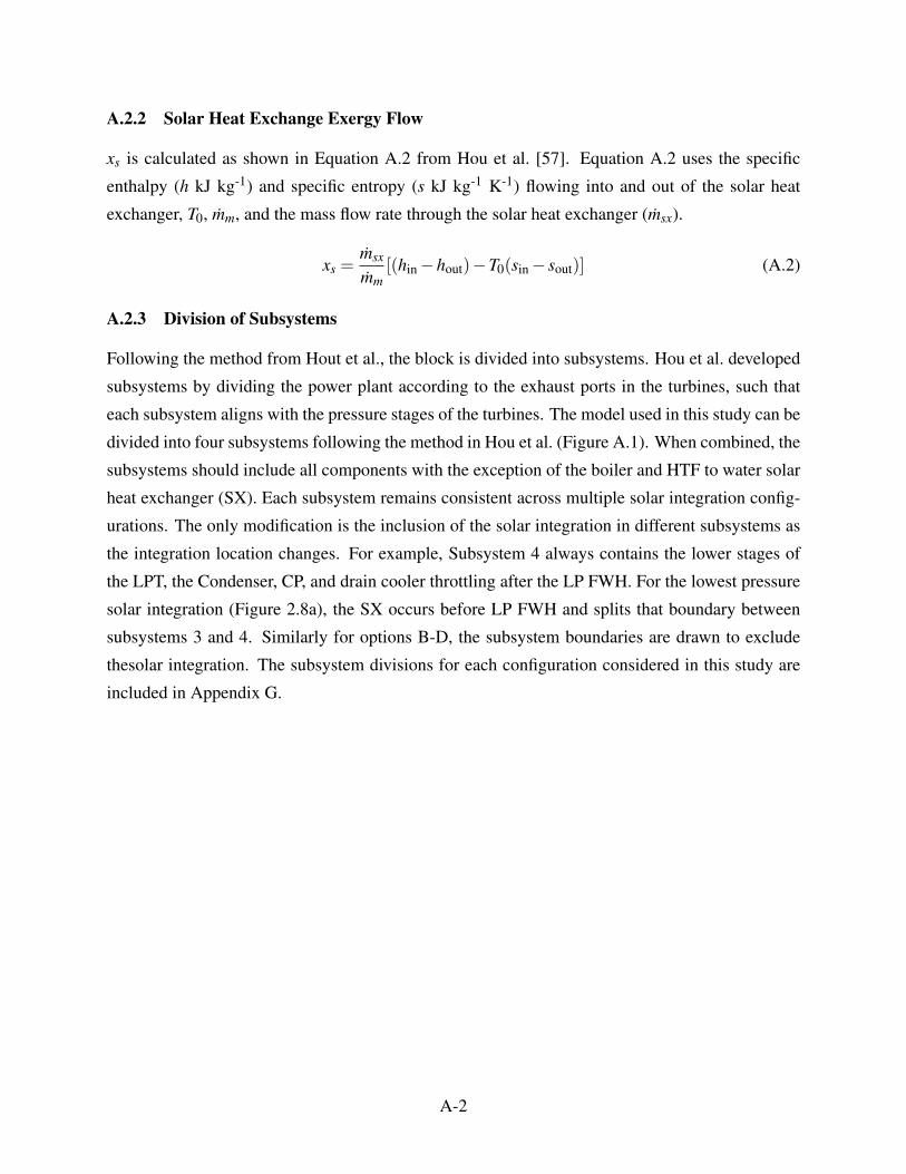
A.2.2 Solar Heat Exchange Exergy Flow
xs is calculated as shown in Equation A.2 from Hou et al. [57]. Equation A.2 uses the specific
enthalpy (h kJ kg-1) and specific entropy (s kJ kg-1 K-1) flowing into and out of the solar heat
exchanger, T0, mm, and the mass flow rate through the solar heat exchanger (msx).
xs =msx
mm[(hin−hout)−T0(sin− sout)] (A.2)
A.2.3 Division of Subsystems
Following the method from Hout et al., the block is divided into subsystems. Hou et al. developed
subsystems by dividing the power plant according to the exhaust ports in the turbines, such that
each subsystem aligns with the pressure stages of the turbines. The model used in this study can be
divided into four subsystems following the method in Hou et al. (Figure A.1). When combined, the
subsystems should include all components with the exception of the boiler and HTF to water solar
heat exchanger (SX). Each subsystem remains consistent across multiple solar integration config-
urations. The only modification is the inclusion of the solar integration in different subsystems as
the integration location changes. For example, Subsystem 4 always contains the lower stages of
the LPT, the Condenser, CP, and drain cooler throttling after the LP FWH. For the lowest pressure
solar integration (Figure 2.8a), the SX occurs before LP FWH and splits that boundary between
subsystems 3 and 4. Similarly for options B-D, the subsystem boundaries are drawn to exclude
thesolar integration. The subsystem divisions for each configuration considered in this study are
included in Appendix G.
A-2
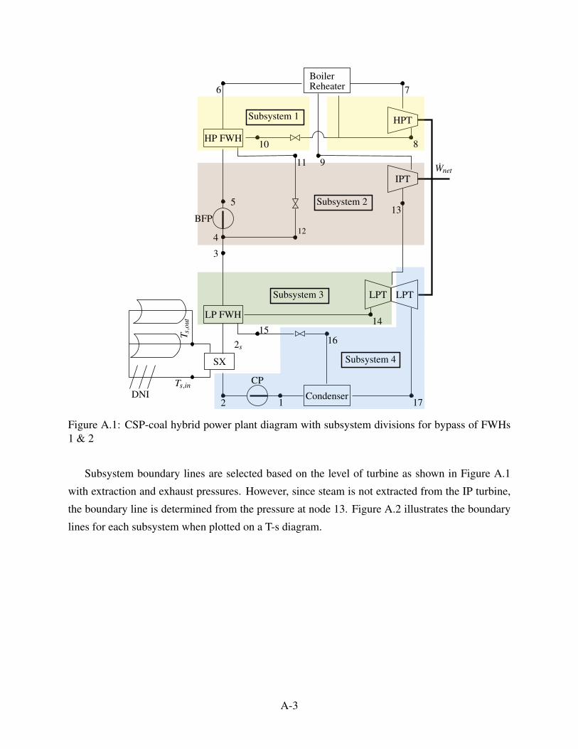
1
5
6
9
10
14
12
13
17
BFP
CP
4
3
1516
LPT
2
HP FWH
LP FWH
LPT
IPT
HPT
Condenser
7
8
11
BoilerReheater
Wnet
2s
T s,o
ut
Ts,in
SX Subsystem 4
Subsystem 3
Subsystem 2
Subsystem 1
DNI
Figure A.1: CSP-coal hybrid power plant diagram with subsystem divisions for bypass of FWHs1 & 2
Subsystem boundary lines are selected based on the level of turbine as shown in Figure A.1
with extraction and exhaust pressures. However, since steam is not extracted from the IP turbine,
the boundary line is determined from the pressure at node 13. Figure A.2 illustrates the boundary
lines for each subsystem when plotted on a T-s diagram.
A-3

0 2 4 6 8
Entropy [kJ kg-1
K-1
]
300
400
500
600
700
800
900
Te
mp
era
ture
[K
]
Subsystem 1
Subsystem 2
Subsystem 3
Subsystem 4
P10
P13
P14
Figure A.2: Temperature vs entropy plot of main loop of CSP-coal hybrid power plant subsystems.
A.2.4 Calculation of Solar Proportion of Work Output
Once subsystems are determined, the next step is to calculate the solar proportion of work out-
put (rs). Equation A.3 defines rs as the ratio of reversible solar work output (ws,rev) to the total
reversible work output (wrev) where wrev is the sum of ws,rev and the coal work output w f ,rev.
rs =ws,rev
wrev=
ws,rev
ws,rev + w f ,rev(A.3)
Hou et al. [57] defines ws,rev and w f ,rev as the integral of the temperature curve through the
solar heat exchange and the boiler respectively. Using the equations for reversible work assumes
that the heat transfer out of the subsystem is negligible compared to the irreversibilities contained
within the subsystem. Equations A.4 and A.5 demonstrate the process to calculate ws,rev and w f ,rev
respectively. Figure A.3 illustrates this process for subsystem 3.
ws,rev,i =ms
mm
∫ Ss,2
Ss,1
[Ti−1(s)−Ti(s)]ds (A.4)
A-4

w f ,rev,i =
∫ S7S6[Ti−1(s)−Ti(s)]ds i = 1
w f ,rev,i =∫ S7
S6[Ti−1(s)−Ti(s)]ds+ mrh
mm
∫ S9S8[Ti−1(s)−Ti(s)]ds i = 2,3,4
(A.5)
0 2 4 6 8
Entropy [kJ kg-1
K-1
]
300
400
500
600
700
800
900
Tem
pera
ture
[K
]
Subsystem 1
Subsystem 2
Subsystem 3
Subsystem 4
Ss,1
Ss,2
S6
S7
S8
S9
Pi-1
Pi
Subsystem 1
Subsystem 2
Subsystem 3
Subsystem 4
Figure A.3: Temperature vs entropy plot of main loop of CSP-coal hybrid power plant subsystemsdemonstrating the calculation of reversible work for subsystem i
Figure A.3 illustrates the process for calculating reversible work for subsystem 3 bounded by
P9 and P14 The boundary line between subsystems 1 and 2 varies due to the throttle between nodes
8 and 10. Since P8 is different than P10, Pi for subsystem 2 is equal to P8 before the throttle and is
throttled down to equal P10 after the throttle. This allows for the temperature curve to account for
the throttling between nodes 8 and 10.
Since the solar integration site changes, the location of Ss,1 and Ss,2 is subject to change. For
the scenario that the solar exchange occurs after node 6, S6 would be adjusted to be equal to Ss,2.
Equations A.4 and A.5 are applied by using the trapezoid rule to estimate the area under the
temperature curves for each constant pressure boundary line. The upper boundary curve for sub-
system 1 cannot be represented by a constant pressure line because of the pressure drop across the
boiler. To account for the pressure drop in subsystem 1, w f ,rev is determined by setting it equal
A-5
to the heat transferred into the water from the boiler. This process is justified by rearranging the
entropy balance and energy balance equations to solve for heat transferred into the boiler [45].
The process for determining the heat transferred into the boiler q is demonstrated in Equation A.6
where T is the temperature curve through the boiler and upper boundary line for subsystem 1.
q =∫
T (s)ds = h7−h6 (A.6)
Equation A.6 shows that q is equal to the integral under the temperature curve through the boiler
which allows for w f ,rev to be determined for subsystem 1 by finding the difference between q
and the area under the lower boundary line of subsystem 1. Equation A.7 solves for w f ,rev by
substituting Equation A.6 for the integral over Ti−1(s) in Equation A.4. For Equation A.7, Ti(s) is
the temperature curve for the the lower boundary line of subsystem 1.
w f ,rev = h7−h6−∫ s7
s6
Ti(s)ds (A.7)
A.2.5 Calculation of Exergy Destruction
Exergy destruction is calculated by treating each subsystem as a control volume and performing
an exergy balance. Equation A.8 expresses the exergy balance for steady flow systems where T0
is the dead state temperature, Tk is the boundary temperature, Qk is the rate of heat crossing the
boundary at Tk, Wout is the rate that work crosses the boundary line, Xin and Xout are respectively
exergy entering and leaving the subsystem through mass flow, and Xd is the exergy destroyed [45].
Qk is assumed to be entering and Wout is assumed to be leaving the subsystem.
N
∑k(1− T0
Tk)Qk−Wout + Xin− Xout− Xd = 0 (A.8)
The only subsystem that has a value for Qb is subsystem 4 as a result of the condenser, however
it is assumed that T0 = Tb for the condenser to include all irreversibilities in the system. Work
leaving each subsystem can be devided into work leaving through the turbine (Wt) and entering
through the pump (Wp). Equation A.8 is simplified to solve for Xd .
Xd = Xin− Xout +Wp−Wt (A.9)
It is important to note that each of the subsystems have multiple mass flow rates (m) crossing
the boundary line. For example, in subsystem 2 m through the IPT is different than m through the
BFP. To allow for the value of Xd in each subsystem to be considered for the solar contribution of
A-6
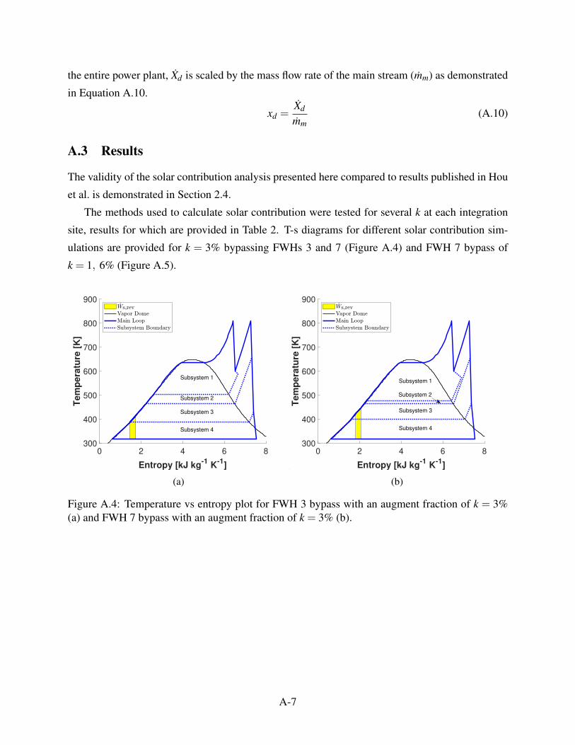
the entire power plant, Xd is scaled by the mass flow rate of the main stream (mm) as demonstrated
in Equation A.10.
xd =Xd
mm(A.10)
A.3 Results
The validity of the solar contribution analysis presented here compared to results published in Hou
et al. is demonstrated in Section 2.4.
The methods used to calculate solar contribution were tested for several k at each integration
site, results for which are provided in Table 2. T-s diagrams for different solar contribution sim-
ulations are provided for k = 3% bypassing FWHs 3 and 7 (Figure A.4) and FWH 7 bypass of
k = 1, 6% (Figure A.5).
0 2 4 6 8
Entropy [kJ kg-1
K-1
]
300
400
500
600
700
800
900
Te
mp
era
ture
[K
]
Subsystem 1
Subsystem 2
Subsystem 3
Subsystem 4
(a)
0 2 4 6 8
Entropy [kJ kg-1
K-1
]
300
400
500
600
700
800
900T
em
pe
ratu
re [
K]
Subsystem 1
Subsystem 3
Subsystem 4
Subsystem 2
(b)
Figure A.4: Temperature vs entropy plot for FWH 3 bypass with an augment fraction of k = 3%(a) and FWH 7 bypass with an augment fraction of k = 3% (b).
A-7
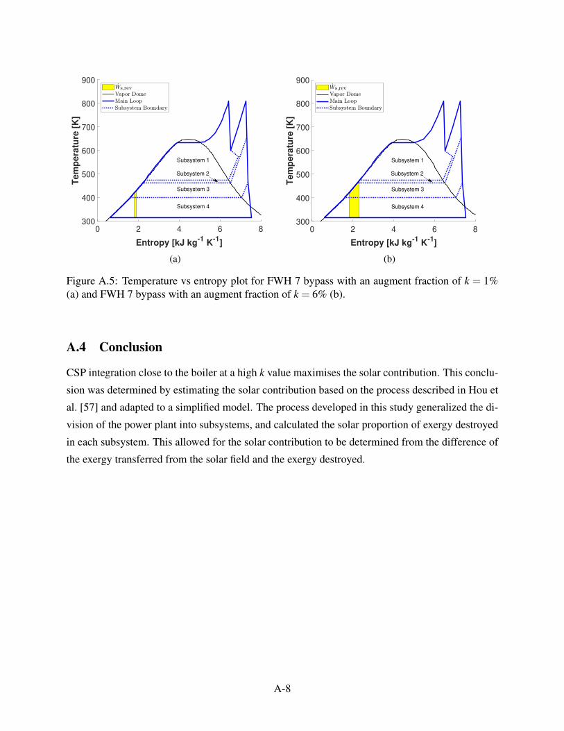
0 2 4 6 8
Entropy [kJ kg-1
K-1
]
300
400
500
600
700
800
900T
em
pe
ratu
re [
K]
Subsystem 1
Subsystem 3
Subsystem 4
Subsystem 2
(a)
0 2 4 6 8
Entropy [kJ kg-1
K-1
]
300
400
500
600
700
800
900
Tem
pera
ture
[K
]
Subsystem 1
Subsystem 3
Subsystem 4
Subsystem 2
(b)
Figure A.5: Temperature vs entropy plot for FWH 7 bypass with an augment fraction of k = 1%(a) and FWH 7 bypass with an augment fraction of k = 6% (b).
A.4 Conclusion
CSP integration close to the boiler at a high k value maximises the solar contribution. This conclu-
sion was determined by estimating the solar contribution based on the process described in Hou et
al. [57] and adapted to a simplified model. The process developed in this study generalized the di-
vision of the power plant into subsystems, and calculated the solar proportion of exergy destroyed
in each subsystem. This allowed for the solar contribution to be determined from the difference of
the exergy transferred from the solar field and the exergy destroyed.
A-8
B State Properties
Simulating the performance of the simplified model requires multiple input values, relationships,
and equations relating to equipment performance or operating behavior of the hardware being
modeled. A derivative of the state postulate requires two independent, intensive properties to fix
the state of a simple compressible system [45]. Thus, for each state in the representative model,
two properties that are independent of each other and do not depend on mass (intensive) must be
provided to determine the other properties of interest at that state.
For the model presented in this work, we are particularly interested in the following properties.
• Pressure (P [MPa])
• Temperature (T [K])
• Specific enthalpy (h [kJ kg-1])
• Specific entropy (s [kJ kg-1 K-1])
• Steam quality (x) mvapormtotal
The information required to obtain these properties can be separated into four categories
1. Correlation provided by user (Table F.1)
2. Process design points
3. Conservation of energy
4. Efficiency
We have selected the HPT 1st stage pressure as the control parameter used to adjust the power
generation of the plant. Because this pressure is the independent variable, all correlations (category
1) used to calculate the properties for the simulation of the Hunter plant are related to the HPT 1st
stage pressure (Table F.1).
The description of state point values are provided sequentially below beginning with state 1.
When the properties of a state are dependent on a process related to a later state, some conditions
are introduced out of order.
The pressure at state 1 is equivalent to the condenser operating pressure, provided as a correla-
tion in Table F.1 (category 1). The water in condensers is designed to exit as a saturated liquid, so
the second property to fix state 1 is x = 0 (category 2).
The feedwater in the condensate stage of real power plants incrementally increases in pressure
as it is heated until it enters the DA. In the simplified model, the condensate stage is assumed to take
place at constant pressure (P2 = P3 = P4), as opposed to the gradual compression experienced in
the real plant. This pressure is approximated using a correlation in Table F.1 for the DA extraction
pressure (category 1). The CP is assumed to have a constant isentropic efficiency. The isentropic
efficiency of a pump is defined as the ratio of the isentropic work (∆s = 0) to the actual work. For
B-1
pumps with an outlet enthalpy (he) and inlet enthalpy (hi), the work done by that pump can be
derived from conservation of energy to get Equation B.1.
Wpump = m(he−hi) (B.1)
The isentropic efficiency can then be written in terms of the actual work (Wa) and isentropic work
(Ws) in Equaion B.2.
ηpump =Ws
Wa=
he,s−hi
he,a−hi(B.2)
After finding the isentropic enthalpy of state 2 (he,s = h(P2,s1)), the actual enthalpy can be calcu-
lated using the isentropic efficiency (Equation B.2), which fixes state 2 (category 4).
The enthalpy of state 3 is determined using the FWH efficiency. This method can be written in
terms of states 2, 14, and 15 in Equation B.3 (category 2).
h3 =ηFWH
m14(h14−h15)+h(2) (B.3)
State 3 is then fixed knowing h3 and that P3 = P2, as stated previously (category 2).
State 4 is a simplified model of the DA used in coal plants to remove air from the feedwater
before it enters the boiler. The ideal version of a DA is a mixing chamber. In the case of state 4,
condensate stream 3 and FWH drain exit (state 12) enter the chamber at equal pressure and exit at
the same pressure (P3 = P4 = P12, category 2). State 4 is fixed after finding the enthalpy of state 4
using the conservation of energy (category 3). For a steady, open system with no external heating
or work interactions, N inlet streams, and M exit streams,
M
∑j(m jh j)exit =
N
∑k(mkhk)in (B.4)
and, therefore,
h4 =1
m4(m3h3 + m12h12) (B.5)
However, h12 is still unknown for this process. In order to calculate states 4, 11, and 12, a
temperature for state 5 is assumed and used with a correlation for pressure in Table F.1 (category 1)
to fix the state. The temperature for state 11 is determined using the Drain Cooler (DC) temperature
difference specification for FWHs. The DC approach assumes that the drain of the FWH exits at
a specified temperature difference above the feedwater inlet temperature. In the case of the HP
FWH, T11 can be related to the assumed T5 using Equation B.6 (category 2).
B-2

T11 = T5 +DC (B.6)
It is assumed that the steam exits the FWH for state 11 at the same pressure as the extraction inlet
(P11 = P10, category 2). State 11 is then fixed and can be used to determine state 12.
It has been identified previously that state 12 is at the same pressure as states 3 and 4. A
relationship for the throttling process is useful to fix state 12 (category 3). A general expression
for a control volume at steady state with no external heating or work interactions is presented in
Equation B.5. Equation B.7 shows the results for a single inlet and exit. Since m12 = m11, the
enthalpy at states 11 and 12 are equivalent.
M
∑j(m jh j)exit =
N
∑k(mkhk)in (B.7)
State 4 is then fixed as previously described and can be used to evaluate the assumed T5. The
new state 5 is fixed using the boiler feed pump (BFP) efficiency (category 4), as described for
state 2 (Equation B.2) and a pressure calculated from a correlation in Table F.1 (category 1). The
temperature from the new state 5 is compared to the assumed state. A tolerance of 0.1% is applied
for sensitivity when comparing the assumed and calculated state 5 temperatures. The properties of
the calculated state 5 are then used to iterate through the calculations for states 4, 11, and 12 until
the tolerance requirement is met.
State 6 is calculated assuming a FWH efficiency (ηFWH) based on the conservation of energy
(category 3). For a FWH, the amount of energy transferred between the streams can be determined
by analyzing the heat transfer material, or the space between the extraction and feedwater streams.
Since the extracted steam and feedwater heat rates are related by ηFWH,
ηFWH m10−11(h10−h11) = m5−6(h6−h5) (B.8)
and, therefore,
h6 = h5 +ηFWHm10−11
m5−6(h10−h11) (B.9)
State 6 can then be fixed using Equation B.9 and the pressure, assuming ηFWH≈ 99%.3 Similar
to the LP FWH, the feedwater exit is assumed to be at the same pressure as the inlet (P6 = P5,
category 2).
State 7 is at the exit of the boiler. For lack of a model for pressure losses in the boiler, a
correlation is provided for the boiler outlet pressure in Table F.1 (category 1). It is assumed that a
3ηFWH = 99% confirmed with operating data from Hunter Unit 3
B-3

boiler operates at constant temperature (category 1).4
The exhaust or extraction properties from a turbine are dependent on turbine pressure limits
and its isentropic efficiency. For the example of the HPT exhaust (state 8), the inlet pressure has
already been calculated (P7). The pressure ratio from the inlet of the HPT to the exhaust varies with
Ps1, but it is assumed that the pressure ratio from Ps1 to the HPT exhaust is constant.5 Since the 1st
stage pressure is set for a plant operating condition, the HPT exhaust pressure can be calculated
using a constant pressure ratio (category 1).
The isentropic efficiency of an adiabatic turbine is similar to Equation B.2 for compressor
efficiency.
ηturb =Wa
Ws=
he,a−hi
he,s−hi(B.10)
For a specified turbine efficiency (category 1), the exit state can be fixed by rearranging Equa-
tion B.10 to solve for he,a (category 4).
The boiler reheating is assumed to be a constant pressure process (P9 = P8, category 2). As
discussed previously, the boiler operates at a consistent temperature, thus it is assumed that T9 = T7
(category 2). As long as the water is not a saturated liquid-vapor mixture, pressure and temperature
are independent and state 9 is fixed.
Multiple options for modeling state 10 have been considered (Appendix C); the selected option
is to throttle a fraction of the steam extracted from the HPT exhaust to the mass-averaged pres-
sure. The process to calculate the mass-averaged pressure is based on a generalized schematic in
Figure B.1.
In the case represented in Figure B.1, there are 3 HP FWHs with a single extraction from the
HPT exhaust (A) and 2 extractions from the IPT (B, C). First, the FWH mass fraction (mf ) is
calculated using a ratio of the respective extraction mass flow rate to the total mass extracted, as in
Equation B.11 for the FWH mass fraction of stream A.
mf A =mA
mA + mB + mC(B.11)
The mass-averaged pressure is assumed to be the combination of each of the individual extraction
pressures (Equation B.12) while the extraction mass flow rate in the simplified model is assumed
to be equal to the sum of the extraction flow rates.
4Data from Hunter Unit 3 confirms constant operating temperature as reported in Table F.1.5The constant Ps1-HPT exhaust pressure ratio is confirmed with data from Hunter Unit 3.
B-4
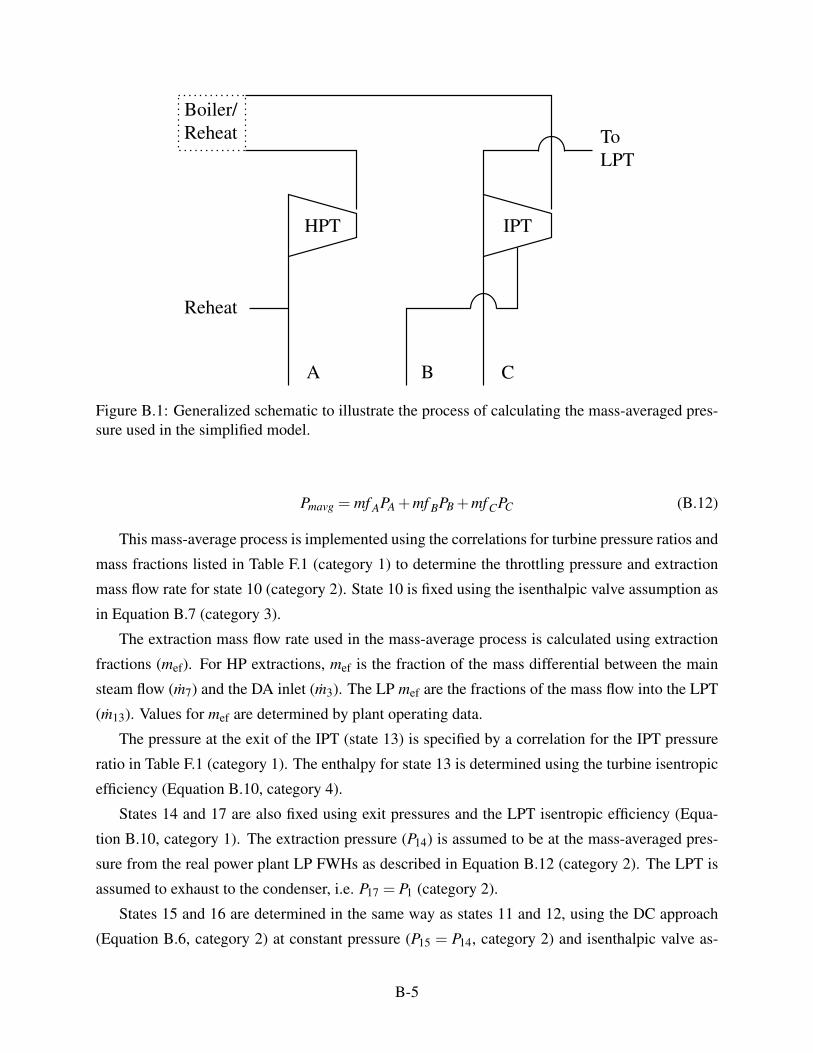
HPT IPT
Boiler/Reheat
A CB
ToLPT
Reheat
Figure B.1: Generalized schematic to illustrate the process of calculating the mass-averaged pres-sure used in the simplified model.
Pmavg = mf APA +mf BPB +mfCPC (B.12)
This mass-average process is implemented using the correlations for turbine pressure ratios and
mass fractions listed in Table F.1 (category 1) to determine the throttling pressure and extraction
mass flow rate for state 10 (category 2). State 10 is fixed using the isenthalpic valve assumption as
in Equation B.7 (category 3).
The extraction mass flow rate used in the mass-average process is calculated using extraction
fractions (mef). For HP extractions, mef is the fraction of the mass differential between the main
steam flow (m7) and the DA inlet (m3). The LP mef are the fractions of the mass flow into the LPT
(m13). Values for mef are determined by plant operating data.
The pressure at the exit of the IPT (state 13) is specified by a correlation for the IPT pressure
ratio in Table F.1 (category 1). The enthalpy for state 13 is determined using the turbine isentropic
efficiency (Equation B.10, category 4).
States 14 and 17 are also fixed using exit pressures and the LPT isentropic efficiency (Equa-
tion B.10, category 1). The extraction pressure (P14) is assumed to be at the mass-averaged pres-
sure from the real power plant LP FWHs as described in Equation B.12 (category 2). The LPT is
assumed to exhaust to the condenser, i.e. P17 = P1 (category 2).
States 15 and 16 are determined in the same way as states 11 and 12, using the DC approach
(Equation B.6, category 2) at constant pressure (P15 = P14, category 2) and isenthalpic valve as-
B-5

sumption (Equation B.7, category 3) exiting at the condenser pressure (P16 = P1, category 2).
In summary, below is a list of inputs the model requires in order to simulate the power plant
performance:
• Condenser pressure
• All FWH extraction pressures
• Boiler inlet pressure
• Boiler outlet pressure
• Boiler operating temperature
• Boiler inlet mass flow rate
• DA inlet water mass flow rate
• Extraction fractions for each FWH
• HPT 1st stage-exhaust pressure ratio
• HPT, IPT, LPT isentropic efficiencies
• IPT, LPT extraction pressure ratios
B-6

C HP FWH Extraction
C.1 Overview
Combining multiple FWHs from a plant schematic into a single FWH in the representative model
simplifies calculations but creates a problem in calculating properties of the extraction steam. The
extraction pressure is calculated using a mass averaged approach as has been discussed. One other
property must be known in order to determine the other properties of the extraction state. Each
state in the representative model is determined by correlations to actual plant data and by operating
relationships for the hardware to which the state relates. In the case of the HP FWH extraction
steam, knowing the pressure from the mass averaged approach is insufficient; the extraction loca-
tion within the cycle must also be known.
C.2 Methods
Each coal plant has a unique FWH configuration, varying the number of heaters, extraction loca-
tions, and extraction pressures. However, HP FWHs are always operated using steam extracted
from either the HPT or IPT. Thus, extraction from the HPT or IPT is considered for the repre-
sentative model. Specifically, the following options were considered for FWH extraction and are
illustrated in Figure C.1:
1. HPT exhaust at HPT exhaust pressure (Figure C.1a)
2. HPT exhaust throttled to mass averaged pressure (Figure C.1b)
3. IPT extraction at mass averaged pressure (Figure C.1c)
Using steam at the HPT exhaust pressure is infeasible because there would be no difference in
plant performance when the FWH number from the real plant is changed. Thus, results from op-
tions 2 and 3 will be reported and discussed in terms of accuracy and computational performance.
C.3 Results
The remaining design options (Figures C.1b and C.1c) were simulated using the solar integration
model for the Hunter Plant (Appendix H.2) assuming an augment fraction k = 0 and no FWH
bypass. State 10 for option 2 is modeled using an isenthalpic valve to throttle the extracted HPT
exhaust steam to the mass averaged pressure calculated from the plant data. For option 3, the
enthalpy at state 10 is calculated using the isentropic efficiency of the IPT and the same mass
averaged pressure. Results for these tests are provided in Table C.1.
C-1

1
5
6
910
14
12
13
BFP
CP
4
3
15
16
LPT
2
HP FWH
LP FWH
LPT
IPT
HPT
Condenser
7
8
11
BoilerReheater
Wnet
(a)
1
5
6
9
10
14
12
13
17
BFP
CP
4
3
1516
LPT
2
HP FWH
LP FWH
LPT
IPT
HPT
Condenser
7
8
11
BoilerReheater
Wnet
(b)
1
5
6
9
10
14
12
13
17
BFP
CP
4
3
1516
LPT
HP FWH
LP FWH
LPT
IPT
HPT
Condenser
7
8
11
BoilerReheater
Wnet
2
(c)
Figure C.1: Schematics for the three options considered for HP FWH extraction modeling: (a)HPT exhaust pressure, (b) throttled steam extracted from HPT exhaust, and (c) extraction fromIPT.
C-2
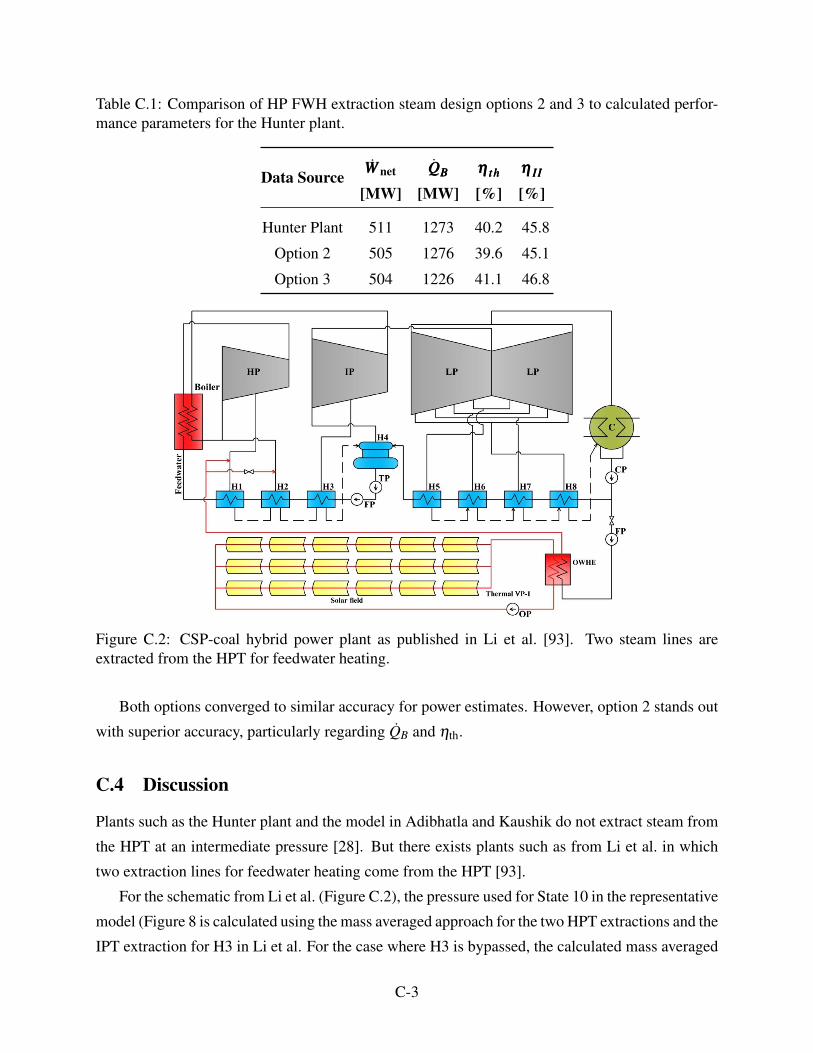
Table C.1: Comparison of HP FWH extraction steam design options 2 and 3 to calculated perfor-mance parameters for the Hunter plant.
Data Source WWW net
[MW]QQQBBB
[MW]ηηη ttthhh
[%]ηηη IIIIII
[%]
Hunter Plant 511 1273 40.2 45.8
Option 2 505 1276 39.6 45.1
Option 3 504 1226 41.1 46.8
Figure C.2: CSP-coal hybrid power plant as published in Li et al. [93]. Two steam lines areextracted from the HPT for feedwater heating.
Both options converged to similar accuracy for power estimates. However, option 2 stands out
with superior accuracy, particularly regarding QB and ηth.
C.4 Discussion
Plants such as the Hunter plant and the model in Adibhatla and Kaushik do not extract steam from
the HPT at an intermediate pressure [28]. But there exists plants such as from Li et al. in which
two extraction lines for feedwater heating come from the HPT [93].
For the schematic from Li et al. (Figure C.2), the pressure used for State 10 in the representative
model (Figure 8 is calculated using the mass averaged approach for the two HPT extractions and the
IPT extraction for H3 in Li et al. For the case where H3 is bypassed, the calculated mass averaged
C-3

pressure would only consider the HPT extractions and would necessarily be greater than the inlet
pressure to the IPT. This eliminates Option 3 for use in systems with multiple HPT extractions. Due
to this complication and the frequency of configurations similar to Li et al., option 2 is selected to
ensure this process can still be widely accessible.
C.5 Conclusion
Option 2 has been shown to be more accurate and option 3 has been shown to be infeasible for
common configurations of coal power plants. Projects with a single HPT extraction line that require
greater modeling accuracy may choose to analyze their system using the approach laid out in option
3. To preserve the scope of this study, option 2 was used for the analysis in this study.
C-4
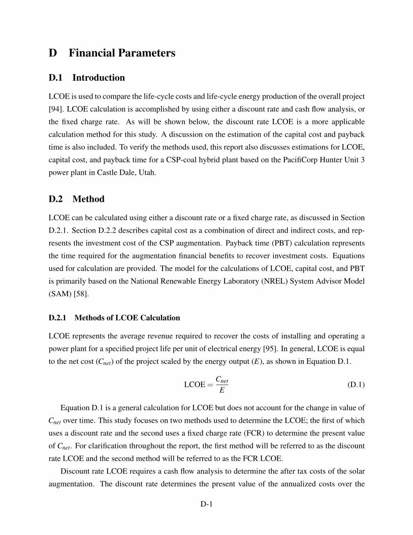
D Financial Parameters
D.1 Introduction
LCOE is used to compare the life-cycle costs and life-cycle energy production of the overall project
[94]. LCOE calculation is accomplished by using either a discount rate and cash flow analysis, or
the fixed charge rate. As will be shown below, the discount rate LCOE is a more applicable
calculation method for this study. A discussion on the estimation of the capital cost and payback
time is also included. To verify the methods used, this report also discusses estimations for LCOE,
capital cost, and payback time for a CSP-coal hybrid plant based on the PacifiCorp Hunter Unit 3
power plant in Castle Dale, Utah.
D.2 Method
LCOE can be calculated using either a discount rate or a fixed charge rate, as discussed in Section
D.2.1. Section D.2.2 describes capital cost as a combination of direct and indirect costs, and rep-
resents the investment cost of the CSP augmentation. Payback time (PBT) calculation represents
the time required for the augmentation financial benefits to recover investment costs. Equations
used for calculation are provided. The model for the calculations of LCOE, capital cost, and PBT
is primarily based on the National Renewable Energy Laboratory (NREL) System Advisor Model
(SAM) [58].
D.2.1 Methods of LCOE Calculation
LCOE represents the average revenue required to recover the costs of installing and operating a
power plant for a specified project life per unit of electrical energy [95]. In general, LCOE is equal
to the net cost (Cnet) of the project scaled by the energy output (E), as shown in Equation D.1.
LCOE =Cnet
E(D.1)
Equation D.1 is a general calculation for LCOE but does not account for the change in value of
Cnet over time. This study focuses on two methods used to determine the LCOE; the first of which
uses a discount rate and the second uses a fixed charge rate (FCR) to determine the present value
of Cnet. For clarification throughout the report, the first method will be referred to as the discount
rate LCOE and the second method will be referred to as the FCR LCOE.
Discount rate LCOE requires a cash flow analysis to determine the after tax costs of the solar
augmentation. The discount rate determines the present value of the annualized costs over the
D-1

project life. FCR LCOE uses the FCR to determine the amount of revenue per dollar of investment
cost that will need to be collected to cover the costs of the investment [96].
Cnet for this study does not account for costs associated with the existing coal plant, rather it
only accounts for the costs the associated with the CSP augmentation. The LCOE of the hybrid
plant can be estimated by the sum of cost of the CSP augmentation and the cost of the existing coal
plant.
Since this study uses a long term analysis, the LCOE is expressed in real dollars rather than
nominal. Real refers to a constant dollar, or an inflation adjusted dollar. This is in contrast to nom-
inal which represents a current dollar value, or a value not adjusted by inflation [58]. Equation D.2
demonstrates the process to convert real rates (rr) to nominal rates (rnom) by using the inflation rate
(ri).
rnom = (ri +1) · (rr +1) (D.2)
Discount Rate LCOE
To generate an accurate LCOE, the net cost is discounted to determine the present value of the
project costs. Equation D.3 uses the nominal discount rate (rd,nom) to determine the present value,
subject to inflation, of Cnet from the after tax costs of the project (Ctot) where N is the analysis
period and n represents the current year. Note that n = 0 represents the initial project investment.
Cnet =N
∑n=0
Cn
(1+ rd,nom)n (D.3)
Discount LCOE is similar to Equation D.1, however Equation D.4 shows that along with the lev-
elized Cnet the real discount rate (rd,r) is applied. Although it appears that E is discounted, the
LCOE is actually the value being discounted. This allows for the money value of the energy load
to be considered at a present day value.
LCOE =Cnet
N∑
n=1
En(1+rr)n
(D.4)
An annualized cash flow analysis is used to determine the variance in Cn over the project life.
The procedure to determine Cn can be separated into four categories: operating expenses, loan
payments, tax credits, and income tax. All formulas for the cash flow analysis, with the exception
of loan payment, were taken from the SAM financial model [58].
Operating and Maintenance Expenses
D-2

Annual operation and maintenance (O&M) expenses (Ctot) include fixed (CFOM) and variable
(CVOM) O&M costs, insurance (Cins), and property tax (Ct,prp). The total expenses for each year
are the sum of the previously mentioned cost values as shown in Equation D.5.
Ctot =CFOM +CVOM +Cins +Ct,prp (D.5)
Loan PaymentsAnnual loan payments are a constant yearly payment that are equal to the sum of the debt interest
and the principle payment. Equation D.6 calculates the principle and interest payment (CP&I) from
the loan rate (rint), initial loan balance (Lnet,0), and loan period (NL) [97].
CP&I =rint ·Lnet,0
1− (1+ rint)NL(D.6)
Tax CreditsTax credits are an important variable when considering renewable energy sources. This study
focuses primarily on the federal Investment Tax Credit (ITC) and Project Tax Credit (PTC). Other
incentives used in the SAM financial model but are not included in this study are: Investment based
incentives, capacity based incentives, and production based incentives [58]. These incentives were
omitted because there is not recent history of them being applicable for CSP in the United States.
ITC is a percentage of the investment for solar energy equipment, and is included in the tax
refund for the year the investment was made. Equation D.7 shows the calculation of the ITC based
off of the capital cost and the ITC rate (rITC).
ITC = CC · rITC (D.7)
The PTC is less relevant for this study since the Consolidated Appropriations Act of 2016
terminated the federal PTC for solar power generation [98]. However, Equation D.8 demonstrates
how to calculate the federal PTC, in the case that it is reinstated or if a similar program is applicable
in other countries, by using the PTC rate (rPTC), the electrical capacity of the solar augmentation
(Ws) and the amount of sunlight hours in a year (365 hsun), where hsun is the multi-year average
daily sunlight hours [hrs day-1]. The PTC is only applied throughout a government specified term.
PTCn = Ws ·365 hsun · rPTC (D.8)
ITC is included in the income tax savings during the first year of the project. PTC is included
in the income tax savings during the duration of time specified by the applicable tax law.
D-3

Income TaxOnce the operating expenses, loan payment, and tax credits have been determined, it is then possi-
ble to calculate the federal and state income taxes. The calculation for both the federal and the state
income taxes are almost identical, however, the state income tax is calculated before the federal
income tax so that the state tax will be considered when calculating federal deductions.
Income taxes, including income tax savings (St), are based on state and federal income tax
rates, depreciation schedule, taxable income, operating expenses, interest payments, and applicable
tax credits. Calculations for St are more thoroughly expressed in the MATLAB code included in
Appendix H and were pulled from SAM [58]; however, equation D.9 shows that in general, it
consists of the sum of ITC, PTC, and federal (St,Fed) and state (St,st) income tax savings.
St = St,Fed +St,st + ITC+PTC (D.9)
After Tax CostsAfter calculating the operating expenses, loan payment, tax credits, and income taxes, Ctot can then
be determined for each year as shown in Equation D.10.
Ctot =Ctot +CP&I−St (D.10)
Input values used to calculate the costs of the project vary depending on the location and the
scale of the project. Default values used in these equations are provided in Table 7.
Fixed Charge Rate LCOEWhen financing is neglected and energy output and O&M costs are assumed to be constant, the
LCOE can be estimated by using the FCR. The FCR is used to estimate the average annual cost of
capital. The benefit to using the FCR method is that it allows for the LCOE to be estimated from
first year inputs without the need for a complete cash flow analysis. This eliminates the possibility
of estimating PBT which is further discussed in Section D.2.2. Equation D.11 estimates the LCOE
by multiplying the FCR by the capital cost (CC). The product of the FCR and CC is added to the
average annual cost which is all scaled by the first year energy output (E0).
LCOE =FCR ·CC+CFOM,0
E0+ rVOM (D.11)
There are two assumptions involved in Equation D.11 that cause it to differ from the discount
LCOE. Since E0 is used instead of a discounted E, the future energy output is not scaled back to
D-4
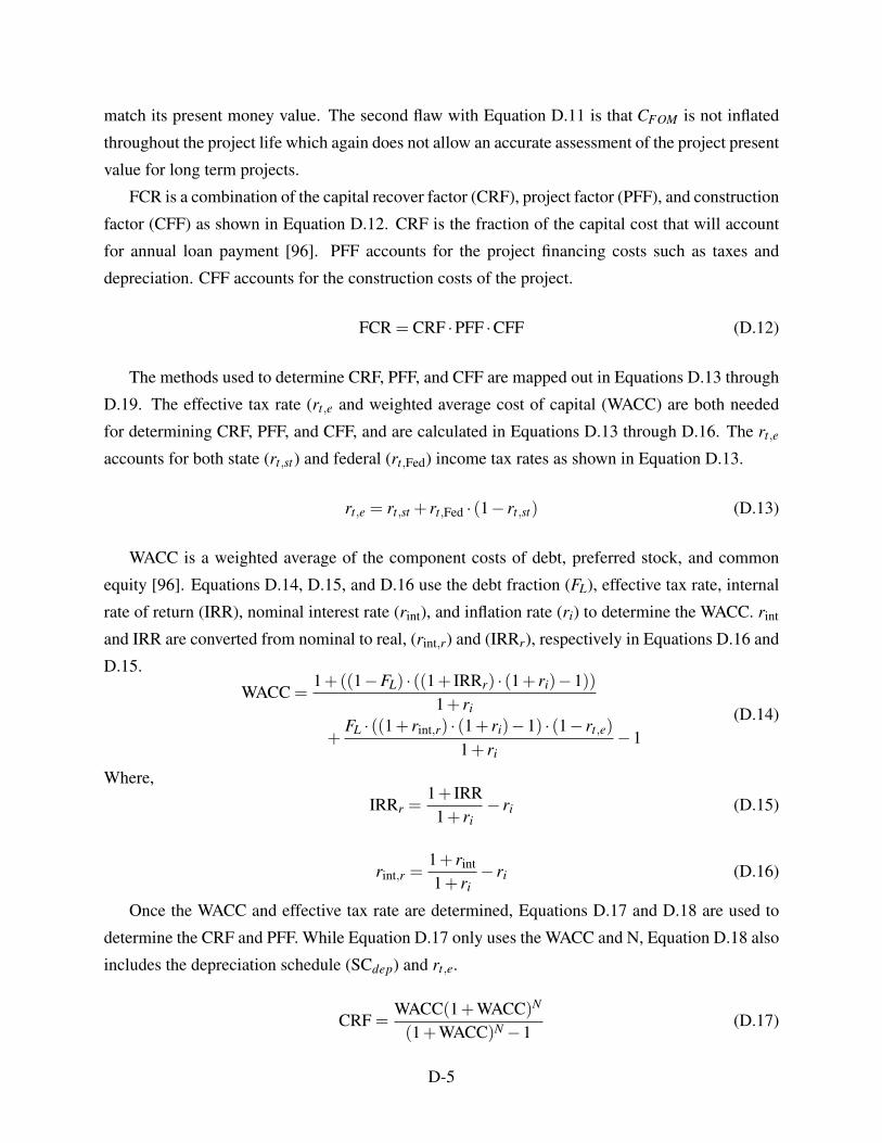
match its present money value. The second flaw with Equation D.11 is that CFOM is not inflated
throughout the project life which again does not allow an accurate assessment of the project present
value for long term projects.
FCR is a combination of the capital recover factor (CRF), project factor (PFF), and construction
factor (CFF) as shown in Equation D.12. CRF is the fraction of the capital cost that will account
for annual loan payment [96]. PFF accounts for the project financing costs such as taxes and
depreciation. CFF accounts for the construction costs of the project.
FCR = CRF ·PFF ·CFF (D.12)
The methods used to determine CRF, PFF, and CFF are mapped out in Equations D.13 through
D.19. The effective tax rate (rt,e and weighted average cost of capital (WACC) are both needed
for determining CRF, PFF, and CFF, and are calculated in Equations D.13 through D.16. The rt,e
accounts for both state (rt,st) and federal (rt,Fed) income tax rates as shown in Equation D.13.
rt,e = rt,st + rt,Fed · (1− rt,st) (D.13)
WACC is a weighted average of the component costs of debt, preferred stock, and common
equity [96]. Equations D.14, D.15, and D.16 use the debt fraction (FL), effective tax rate, internal
rate of return (IRR), nominal interest rate (rint), and inflation rate (ri) to determine the WACC. rint
and IRR are converted from nominal to real, (rint,r) and (IRRr), respectively in Equations D.16 and
D.15.
WACC =1+((1−FL) · ((1+ IRRr) · (1+ ri)−1))
1+ ri
+FL · ((1+ rint,r) · (1+ ri)−1) · (1− rt,e)
1+ ri−1
(D.14)
Where,
IRRr =1+ IRR
1+ ri− ri (D.15)
rint,r =1+ rint
1+ ri− ri (D.16)
Once the WACC and effective tax rate are determined, Equations D.17 and D.18 are used to
determine the CRF and PFF. While Equation D.17 only uses the WACC and N, Equation D.18 also
includes the depreciation schedule (SCdep) and rt,e.
CRF =WACC(1+WACC)N
(1+WACC)N−1(D.17)
D-5

PFF =
1− (rt,e ·Å
N∑
n=0
SCdep,n(1+WACC)·(1+ri)n+1))
ã1− rt,e
(D.18)
Equation D.19 is used to determine the CFF from the construction cost schedule (SCcon), rt,e,
nominal construction financing interest rate (rcon), and construction period in years (Ncon).
CFF =Ncon
∑n=0
SCcon,n · (1+(1− rt,e) · ((1+ rcon)n+ 1
2 −1)) (D.19)
CRF, PFF, and CFF were estimated from the inputs provided in Table D.1 with the exception
of FOC and VOC. The values in Table D.1 were taken from the default values used in SAM.
Table D.1: Default values for FCR LCOE excluded in Table 7
Default Input Value Source
IRR [%/year] 13 [99]
SCcon* [%/year] 80 10 10 [58]
rcon [%/year] 8 [58]
*The construction cost schedule is a vector of percentages of the capital cost thatare used during each year of the construction of the solar augmentation. Thisstudy assumes a three year construction period.
D.2.2 Model and Input Adjustments for Hybridization
SAM was developed to analyze standalone CSP projects. This section will discuss some of the
changes required to allow for the methods used in SAM to be applied to a coal power plant aug-
mented with solar-thermal energy. The areas that require adjustments include capital cost, O&M
costs, and energy output.
Calculation of the Capital CostTotal capital costs are a combination of direct and indirect costs. The process of calculating direct,
indirect, and capital costs are included in Tables D.2 and 7. Both tables show methods and values
provided by SAM [58] and Adibhatla and Kaushik [100]. Some of the direct costs needed to install
a parabolic trough system are based on the total aperture area of the troughs (Section 2.2).
O&M CostsFor a standalone CSP plant, fist year O&M costs CFOM,0 and CVOM,0 would be calculated using the
D-6
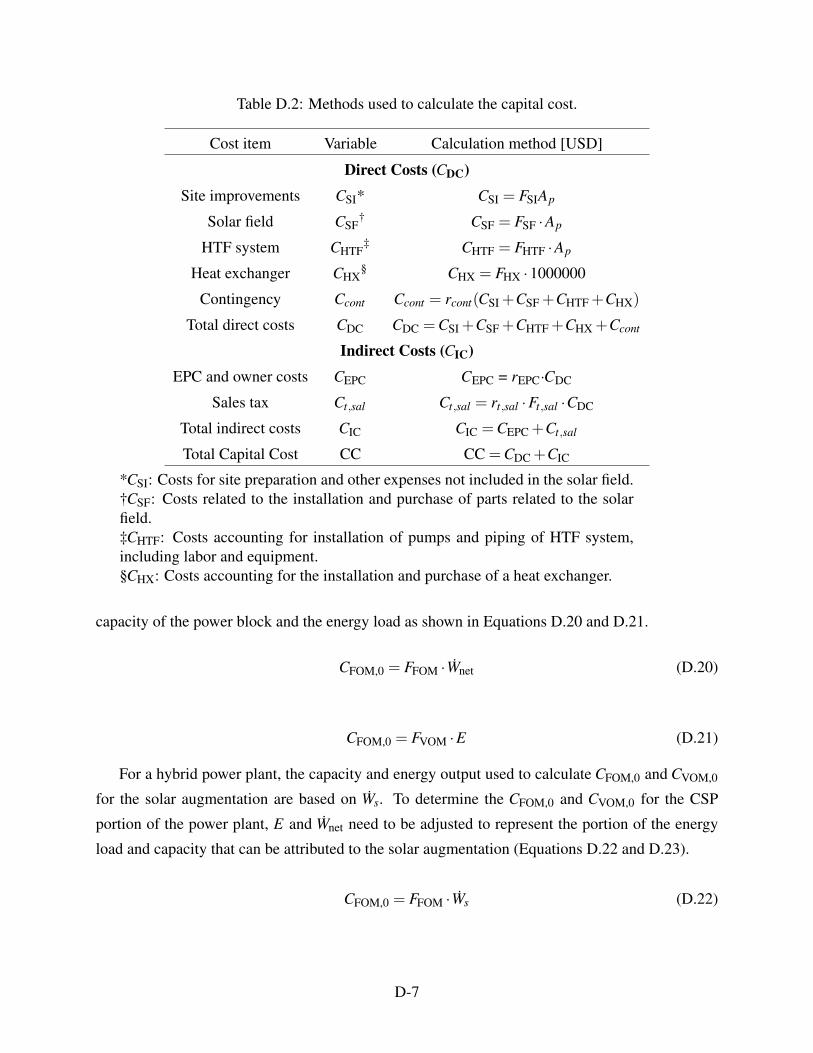
Table D.2: Methods used to calculate the capital cost.
Cost item Variable Calculation method [USD]
Direct Costs (CDC)Site improvements CSI* CSI = FSIAp
Solar field CSF† CSF = FSF ·Ap
HTF system CHTF‡ CHTF = FHTF ·Ap
Heat exchanger CHX§ CHX = FHX ·1000000
Contingency Ccont Ccont = rcont(CSI +CSF +CHTF +CHX)
Total direct costs CDC CDC =CSI +CSF +CHTF +CHX +Ccont
Indirect Costs (CIC)EPC and owner costs CEPC CEPC = rEPC·CDC
Sales tax Ct,sal Ct,sal = rt,sal ·Ft,sal ·CDC
Total indirect costs CIC CIC =CEPC +Ct,sal
Total Capital Cost CC CC =CDC +CIC
*CSI: Costs for site preparation and other expenses not included in the solar field.†CSF: Costs related to the installation and purchase of parts related to the solarfield.‡CHTF: Costs accounting for installation of pumps and piping of HTF system,including labor and equipment.§CHX: Costs accounting for the installation and purchase of a heat exchanger.
capacity of the power block and the energy load as shown in Equations D.20 and D.21.
CFOM,0 = FFOM ·Wnet (D.20)
CFOM,0 = FVOM ·E (D.21)
For a hybrid power plant, the capacity and energy output used to calculate CFOM,0 and CVOM,0
for the solar augmentation are based on Ws. To determine the CFOM,0 and CVOM,0 for the CSP
portion of the power plant, E and Wnet need to be adjusted to represent the portion of the energy
load and capacity that can be attributed to the solar augmentation (Equations D.22 and D.23).
CFOM,0 = FFOM ·Ws (D.22)
D-7

CVOM,0 = FVOMWshsun365 (D.23)
Calculation of Simple Payback TimeWhile LCOE provides important information on the cost of solar and coal hybridization, it does
not provide information on the amount of time it would take to recover the costs. PBT gives further
insight by reporting the time needed to recover associated costs. The definition of PBT can vary
depending on the parameters that are considered and this report focuses on two definitions.
The first definition of PBT (PBT1) is the number of years required for the cumulative fuel
savings (San) to equal the cumulative annual costs (Can) (Equation D.24). San and Can are calculated
by determining the cumulative annual cash flow (Aan) including the capital costs.
Aan = San−Can (D.24)
Equation D.24 is repeated for each year of the project until Aan is equal to 0. The year Aan
is equal to 0 is the projected PBT. It is important to note that Aan includes the capital costs and
neglects the loan payment because this method focuses only on the time required to recover the
initial investment [101].
The second definition of PBT (PBT2) is the time needed for the cumulative fuel savings to
equal the initial investment [101]. Equation D.25 shows that fuel savings (FS) are determined by
converting the fuel offset power (Q f o), applicable only for the time the plant is operating in hybrid
mode (hsun), to the cost of its equivalent coal mass by using the cost (FF ), at 36.3 USD/sh. tn. [102],
and heating value (LHVF) of coal, at 23.9 MJ/kg [103].
FS =365 hsun · Q f o ·FF
LHVF(D.25)
This study only calculates fuel savings as revenue generated from the project, however some
countries implement a carbon tax which, if applicable, would contribute to recovering the costs of
the project. To implement a carbon tax, the tax would be added to the fuel savings. Equation D.26
demonstrates a simple example of how to calculate carbon tax savings (St,CO2) by using a tax rate
(rt,CO2), Esav, the CO2 to coal mass conversion ratio (Fcc), and LHVF.
St,CO2 =rt,CO2 ·Fcc ·Esav
HVF(D.26)
Duffie and Beckman [101] provided a method to calculate PBT2 (Equation D.27) which uses
D-8

0 100 200 300 400
Solar Contribution [MW]
0
500
1000
1500
2000
2500
Ca
pita
l C
ost
[MM
US
D]
CSP Guru Data
CSP Hybrids
Trendline for CSP Guru Data
Financial Model Estimates
Figure D.1: Comparison of capital cost data and calculated capital costs from financial model.
the inflation rate and the capital cost.
PBT2 =ln [CC·ri
FS ]+1ln(1+ ri)
(D.27)
D.3 Results
Actual data for capital costs of CSP power plants is provided by CSP Guru in connection with So-
larPACES [104]. Figure D.1 shows the comparison between the capital costs of actual power plants
and the capital costs estimated using the financial model of this study. The difference between the
values calculated using the financial model and the CSP Guru trend are likely attributed to the
inclusion of all CSP technologies (PTC, LFR, Dish, and Tower) as well as the price of equipment
not considered in the financial model such as turbines, pump for the power block, and a condenser.
Table D.3 was produced using the methods described for calculating LCOE, capital cost, PBT1,
and PBT2, along with the determined input values (Table 7). The model is designed to iterate
based on changes in the net capacity of the power block (Wnet), and the required receiver area (Ar).
D-9

Also included in Table D.3 is the number of the feedwater heater (FWH) that is bypassed and k.
The range for k is 1%, 5%, and the equivalent fraction of that FWH at full operating conditions
(typically 2-3%).
Table D.3: Calculated values for Capital Cost (CC), LCOE, and payback time (PBT).
FWH # k
[%]
AAArrr
[103 m2]
AAAsf
[ac]
CC
[MMUSD]
Discount Rate LCOE
[10-4 USD kWh-1]
FCR LCOE
[10-4 USD kWh-1]
PBT1
[years]
PBT2
[years]
53 6.4 92.1 39.9 4.48 7.6 200 N/A
6 13.3 194.2 80.7 9.11 15 146.4 41.2
10 23.1 337.9 138 16 26 68.35 30
63 6.4 92.1 39.9 4.48 7.62 200 N/A
6 13.3 194.2 80.7 9.12 15 91.5 36.2
10 23.1 337.9 138 16 26 59.9 28.2
73 6.4 92.1 39.9 4.5 7.62 200 N/A
6 13.3 194.2 80.7 9.21 15 90.2 35.2
10 23.1 337.9 138 16 26 61.9 29.5
D.4 Conclusion
Table D.3 demonstrates that the FWH primarily affects the performance of the CSP augmentation,
and k is what primarily affects the LCOE.
The difference in the discount rate and FCR methods for calculating the LCOE are also im-
portant to note. The Discount Rate LCOE varies less than the FCR LCOE and is consistently
separated by about 90%. It is also important to note that the LCOE doesn’t significantly change
for each test. This is most likely a result of scaling by the total energy output of the coal plant
which is very large in comparison to the thermal energy of the CSP.
When comparing the LCOE from the discount rate method and the FCR method, the discount
rate is considered to be more applicable for this study. In addition to providing a cash flow analysis
useful in calculating PBT, discount rate LCOE allows for the present value of future costs to be
considered more accurately. FCR however is less applicable because constant annual costs is a
poor assumption, and future cash flow is not levelized.
D-10
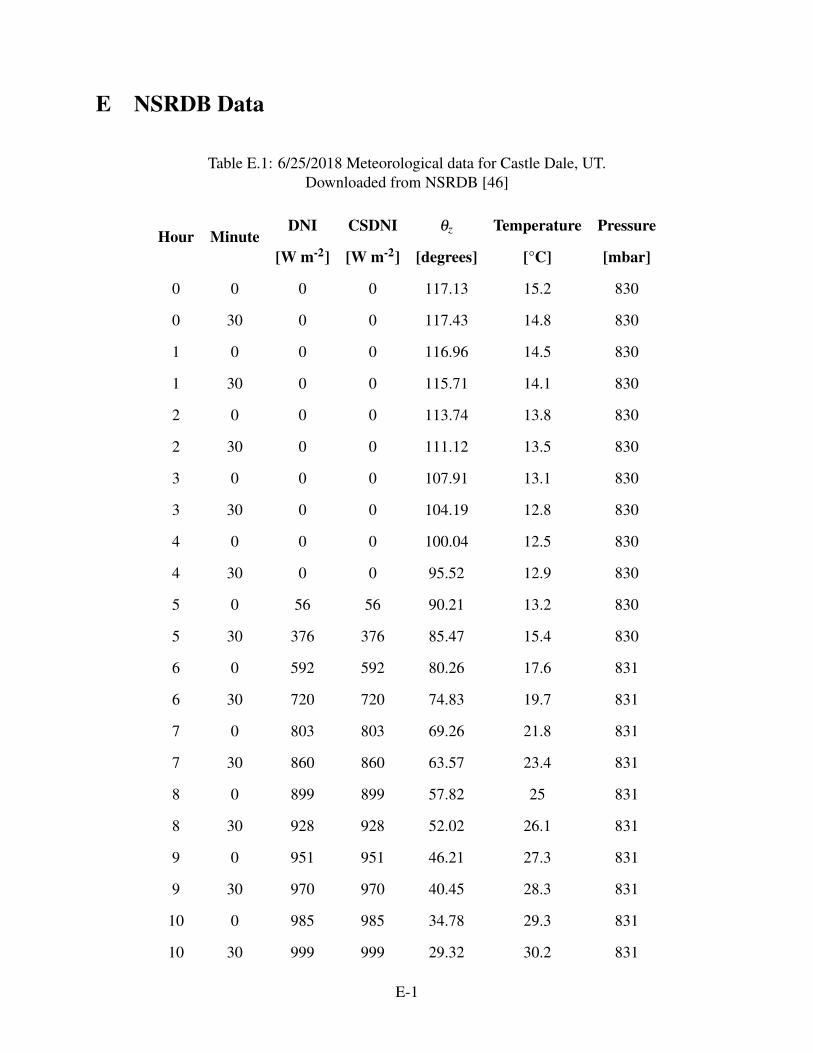
E NSRDB Data
Table E.1: 6/25/2018 Meteorological data for Castle Dale, UT.Downloaded from NSRDB [46]
Hour MinuteDNI
[W m-2]
CSDNI
[W m-2]
θz
[degrees]
Temperature
[°C]
Pressure
[mbar]
0 0 0 0 117.13 15.2 830
0 30 0 0 117.43 14.8 830
1 0 0 0 116.96 14.5 830
1 30 0 0 115.71 14.1 830
2 0 0 0 113.74 13.8 830
2 30 0 0 111.12 13.5 830
3 0 0 0 107.91 13.1 830
3 30 0 0 104.19 12.8 830
4 0 0 0 100.04 12.5 830
4 30 0 0 95.52 12.9 830
5 0 56 56 90.21 13.2 830
5 30 376 376 85.47 15.4 830
6 0 592 592 80.26 17.6 831
6 30 720 720 74.83 19.7 831
7 0 803 803 69.26 21.8 831
7 30 860 860 63.57 23.4 831
8 0 899 899 57.82 25 831
8 30 928 928 52.02 26.1 831
9 0 951 951 46.21 27.3 831
9 30 970 970 40.45 28.3 831
10 0 985 985 34.78 29.3 831
10 30 999 999 29.32 30.2 831
E-1

11 0 1012 1012 24.24 31 831
11 30 1017 1017 19.87 31.7 830
12 0 1020 1020 16.8 32.3 830
12 30 1021 1021 15.82 32.7 830
13 0 1017 1017 17.31 33.1 830
13 30 1012 1012 20.73 33.3 830
14 0 1006 1006 25.3 33.4 830
14 30 998 998 30.48 33.3 830
15 0 986 986 36 33.2 829
15 30 970 970 41.69 32.8 829
16 0 949 949 47.47 32.5 829
16 30 923 923 53.28 32.5 829
17 0 887 887 59.08 31.3 829
17 30 838 838 64.82 30.3 829
18 0 772 772 70.48 29.3 829
18 30 676 676 76.03 26.8 830
19 0 526 526 81.42 24.4 830
19 30 285 285 86.58 23.6 830
20 0 18 18 91.78 22.9 830
20 30 0 0 96.54 22.7 830
21 0 0 0 100.99 22.6 830
21 30 0 0 105.05 22.6 830
22 0 0 0 108.67 22.6 830
22 30 0 0 111.76 22.3 830
23 0 0 0 114.25 22 830
23 30 0 0 116.07 21.3 830
E-2
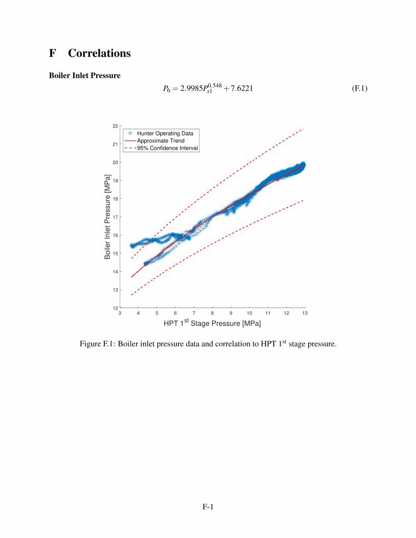
F Correlations
Boiler Inlet PressureP6 = 2.9985P0.548
s1 +7.6221 (F.1)
3 4 5 6 7 8 9 10 11 12 13
HPT 1st
Stage Pressure [MPa]
12
13
14
15
16
17
18
19
20
21
22
Boile
r In
let P
ressure
[M
Pa]
Hunter Operating Data
Approximate Trend
95% Confidence Interval
Figure F.1: Boiler inlet pressure data and correlation to HPT 1st stage pressure.
F-1
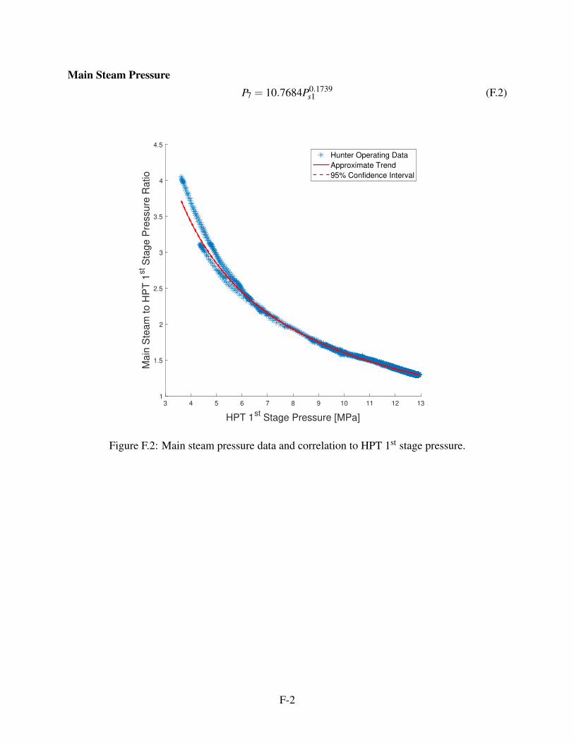
Main Steam PressureP7 = 10.7684P0.1739
s1 (F.2)
3 4 5 6 7 8 9 10 11 12 13
HPT 1st
Stage Pressure [MPa]
1
1.5
2
2.5
3
3.5
4
4.5M
ain
Ste
am
to H
PT
1st S
tage P
ressure
Ratio
Hunter Operating Data
Approximate Trend
95% Confidence Interval
Figure F.2: Main steam pressure data and correlation to HPT 1st stage pressure.
F-2
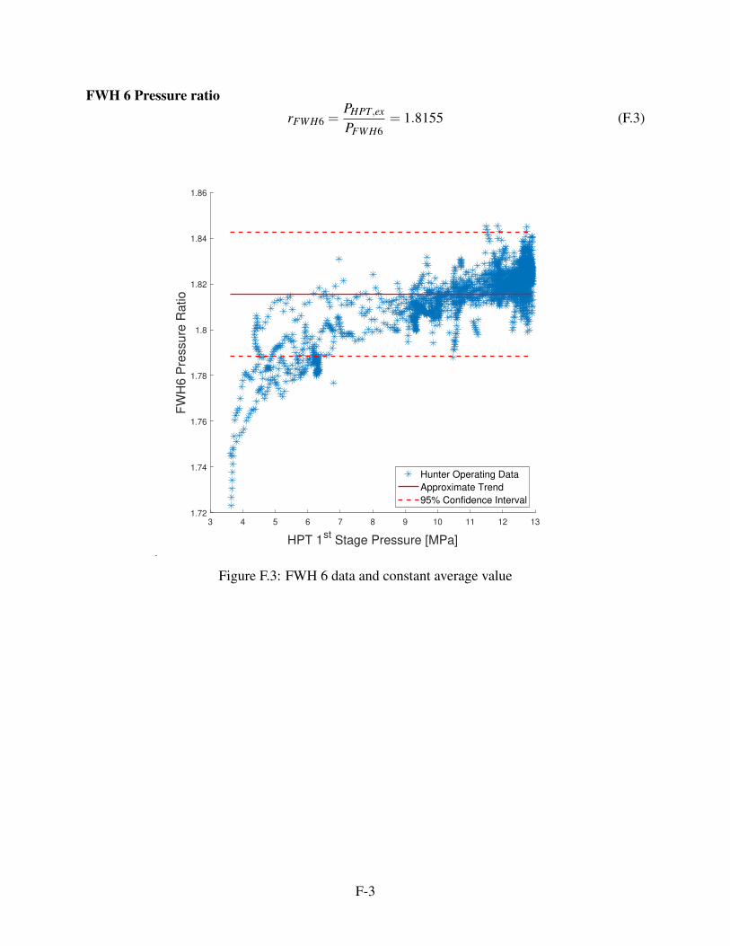
FWH 6 Pressure ratiorFWH6 =
PHPT,ex
PFWH6= 1.8155 (F.3)
3 4 5 6 7 8 9 10 11 12 13
HPT 1st
Stage Pressure [MPa]
1.72
1.74
1.76
1.78
1.8
1.82
1.84
1.86
FW
H6 P
ressure
Ratio
Hunter Operating Data
Approximate Trend
95% Confidence Interval
Figure F.3: FWH 6 data and constant average value
F-3
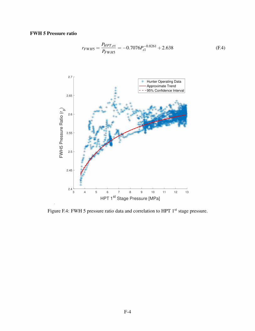
FWH 5 Pressure ratio
rFWH5 =PHPT,ex
PFWH5=−0.7076P−0.8261
s1 +2.638 (F.4)
3 4 5 6 7 8 9 10 11 12 13
HPT 1st
Stage Pressure [MPa]
2.4
2.45
2.5
2.55
2.6
2.65
2.7
FW
H5 P
ressure
Ratio (
r p)
Hunter Operating Data
Approximate Trend
95% Confidence Interval
Figure F.4: FWH 5 pressure ratio data and correlation to HPT 1st stage pressure.
F-4
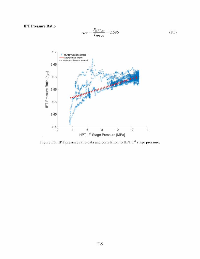
IPT Pressure RatiorIPT =
PHPT,ex
PIPT,ex= 2.586 (F.5)
2 4 6 8 10 12 14
HPT 1st Stage Pressure [MPa]
2.4
2.45
2.5
2.55
2.6
2.65
2.7
IPT
Pre
ssure
Ratio (
r IPT)
Hunter Operating Data
Approximate Trend
95% Confidence Interval
Figure F.5: IPT pressure ratio data and correlation to HPT 1st stage pressure.
F-5

DA Pressure RatiorDA =
PIPT,ex
PDA= 49.7939P−3.4562
s1 +2.2131 (F.6)
3 4 5 6 7 8 9 10 11 12 13
HPT 1st
Stage Pressure [MPa]
2.1
2.2
2.3
2.4
2.5
2.6
2.7
2.8
2.9
DA
Pre
ssure
Ratio (
r DA)
Hunter Operating Data
Approximate Trend
95% Confidence Interval
Figure F.6: DA pressure ratio data and correlation to HPT 1st stage pressure.
F-6
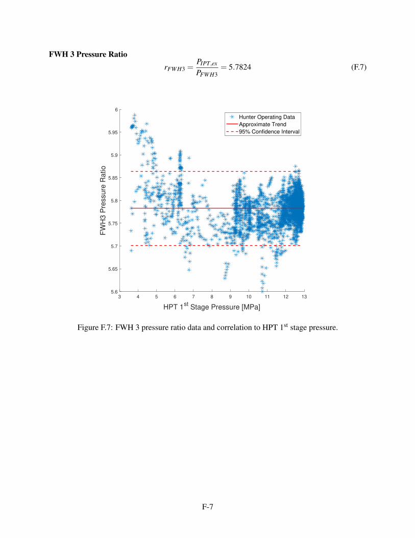
FWH 3 Pressure RatiorFWH3 =
PIPT,ex
PFWH3= 5.7824 (F.7)
3 4 5 6 7 8 9 10 11 12 13
HPT 1st
Stage Pressure [MPa]
5.6
5.65
5.7
5.75
5.8
5.85
5.9
5.95
6
FW
H3 P
ressure
Ratio
Hunter Operating Data
Approximate Trend
95% Confidence Interval
Figure F.7: FWH 3 pressure ratio data and correlation to HPT 1st stage pressure.
F-7
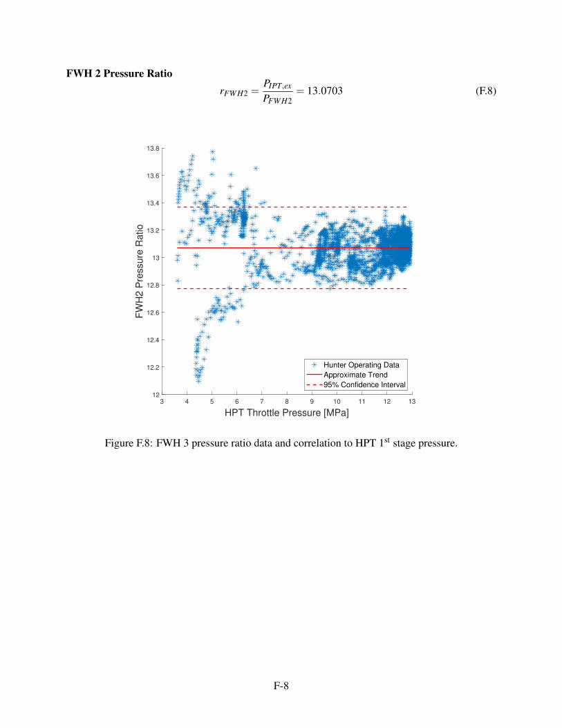
FWH 2 Pressure RatiorFWH2 =
PIPT,ex
PFWH2= 13.0703 (F.8)
3 4 5 6 7 8 9 10 11 12 13
HPT Throttle Pressure [MPa]
12
12.2
12.4
12.6
12.8
13
13.2
13.4
13.6
13.8
FW
H2 P
ressure
Ratio
Hunter Operating Data
Approximate Trend
95% Confidence Interval
Figure F.8: FWH 3 pressure ratio data and correlation to HPT 1st stage pressure.
F-8
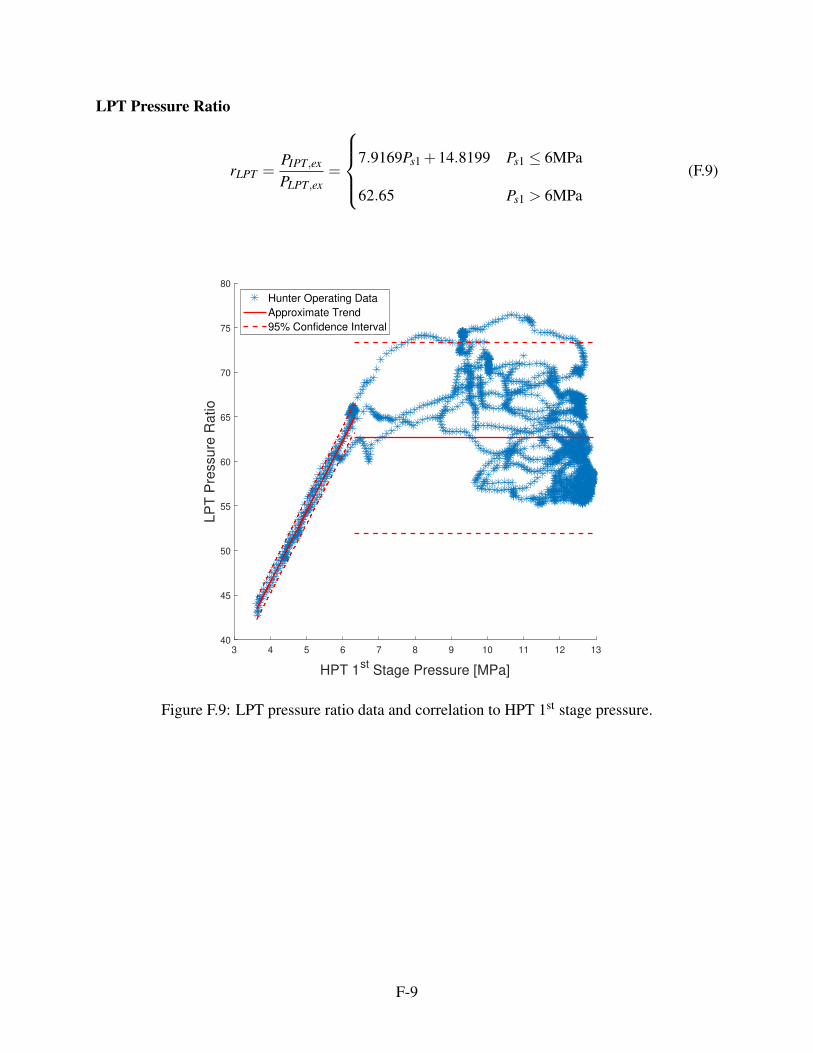
LPT Pressure Ratio
rLPT =PIPT,ex
PLPT,ex=
7.9169Ps1 +14.8199 Ps1 ≤ 6MPa
62.65 Ps1 > 6MPa
(F.9)
3 4 5 6 7 8 9 10 11 12 13
HPT 1st
Stage Pressure [MPa]
40
45
50
55
60
65
70
75
80
LP
T P
ressure
Ratio
Hunter Operating Data
Approximate Trend
95% Confidence Interval
Figure F.9: LPT pressure ratio data and correlation to HPT 1st stage pressure.
F-9
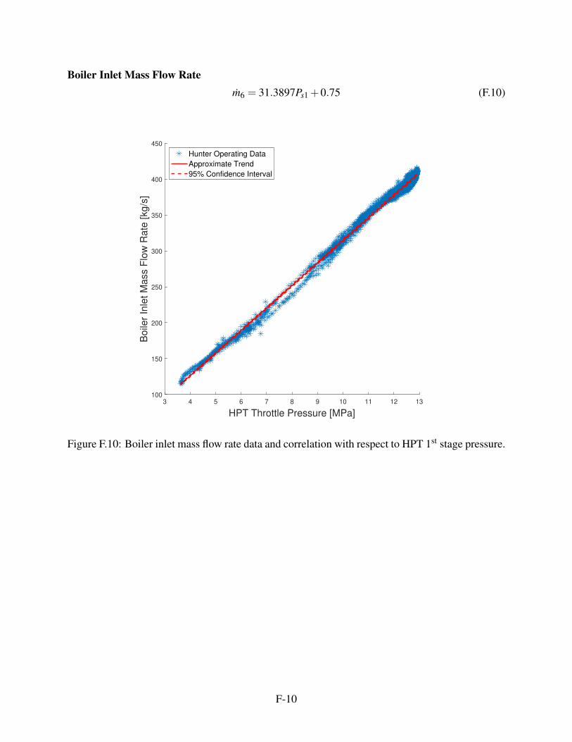
Boiler Inlet Mass Flow Ratem6 = 31.3897Ps1 +0.75 (F.10)
3 4 5 6 7 8 9 10 11 12 13
HPT Throttle Pressure [MPa]
100
150
200
250
300
350
400
450B
oile
r In
let M
ass F
low
Rate
[kg/s
]Hunter Operating Data
Approximate Trend
95% Confidence Interval
Figure F.10: Boiler inlet mass flow rate data and correlation with respect to HPT 1st stage pressure.
F-10
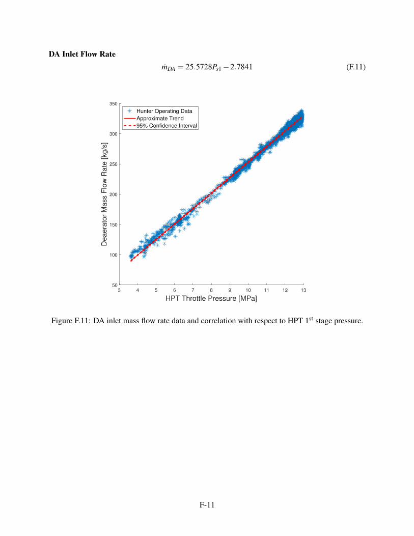
DA Inlet Flow RatemDA = 25.5728Ps1−2.7841 (F.11)
3 4 5 6 7 8 9 10 11 12 13
HPT Throttle Pressure [MPa]
50
100
150
200
250
300
350D
eaera
tor
Mass F
low
Rate
[kg/s
]Hunter Operating Data
Approximate Trend
95% Confidence Interval
Figure F.11: DA inlet mass flow rate data and correlation with respect to HPT 1st stage pressure.
F-11

Tabl
eF.
1:C
orre
latio
npr
oper
tyeq
uatio
nsfo
rus
ein
the
repr
esen
tativ
em
odel
.Pr
oper
ties
gene
rally
follo
wa
pow
erla
wre
latio
nshi
p(P
=aP
b s1+
c)w
here
P s1
isin
MPa
.Con
stan
tpro
pert
ies
are
show
nw
here
a=
b=
0.
Prop
erty
(P)
P 6 [MPa
]r H
PTr F
WH
6r F
WH
5r I
PTr D
Ar F
WH
3r F
WH
2r L
PTm
6
[kg
s-1]
mD
A
[kg
s-1]
T B [K]
P con
d
[MPa
]
ηH
PT
[%]
ηIP
T
[%]
ηL
PT
[%]
aa a2.
9985
10.7
684
0-0
.707
60
49.7
939
00
031
.389
725
.572
80
00
00
bb b0.
548
0.17
390
-0.8
261
0-3
.456
20
00
11
00
00
0
cc c7.
6221
01.
8155
2.68
382.
5860
2.21
315.
7824
13.0
703
62.6
50.
75-2
.784
181
1.8
8.1e
-389
.491
.791
.8
F-12

G Solar Integration Configurations and Subsystems
1
5
6
9
10
14
12
13
17
BFP
CP
4
3
1516
LPT
2
HP FWH
LP FWH
LPT
IPT
HPT
Condenser
7
8
11
BoilerReheater
Wnet
2s
T s,o
ut
Ts,in
SX
DNI
Figure G.1: FWH 1 or FWH 2 bypass solar integration configuration.
G-1
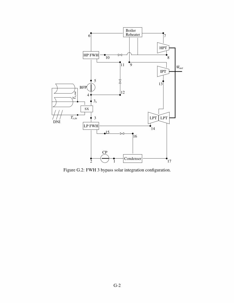
1
5
6
9
10
14
12
13
17
BFP
CP
4
3
1516
LPT
2
HP FWH
LP FWH
LPT
IPT
HPT
Condenser
7
8
11
SX
BoilerReheater
Wnet
3s
T s,o
ut
Ts,inDNI
Figure G.2: FWH 3 bypass solar integration configuration.
G-2
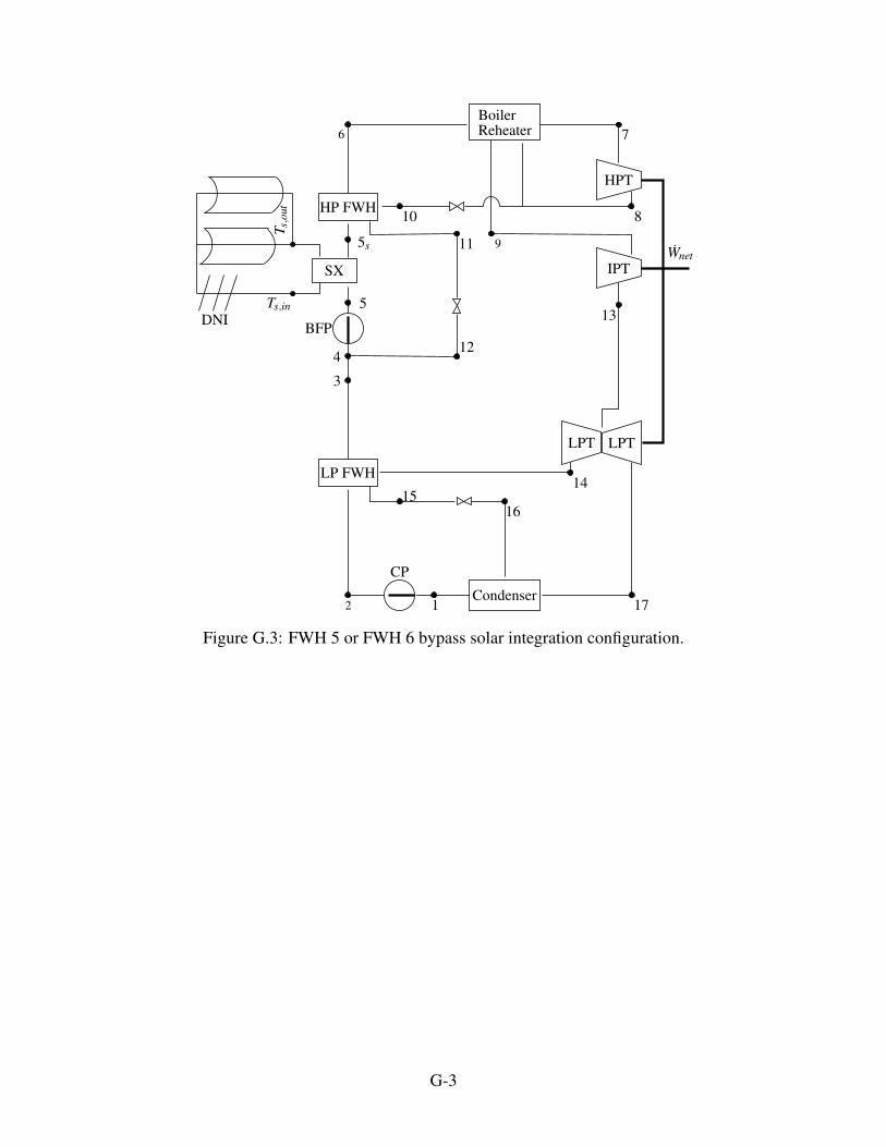
1
5
6
9
10
14
12
13
17
BFP
CP
4
3
1516
LPT
2
HP FWH
LP FWH
LPT
IPT
HPT
Condenser
7
8
11
BoilerReheater
Wnet5s
T s,o
ut
Ts,in
SX
DNI
Figure G.3: FWH 5 or FWH 6 bypass solar integration configuration.
G-3

1
5
6
9
10
14
12
13
17
BFP
CP
4
3
1516
LPT
2
HP FWH
LP FWH
LPT
IPT
HPT
Condenser
7
8
11
SX
BoilerReheater
Wnet
6s
T s,o
ut
Ts,inDNI
Figure G.4: FWH 7 bypass solar integration configuration.
G-4
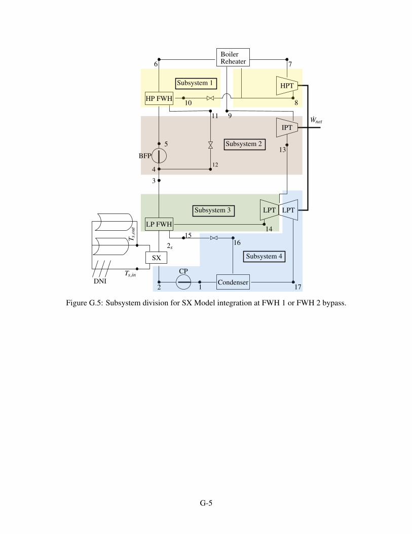
1
5
6
9
10
14
12
13
17
BFP
CP
4
3
1516
LPT
2
HP FWH
LP FWH
LPT
IPT
HPT
Condenser
7
8
11
BoilerReheater
Wnet
2s
T s,o
ut
Ts,in
SX Subsystem 4
Subsystem 3
Subsystem 2
Subsystem 1
DNI
Figure G.5: Subsystem division for SX Model integration at FWH 1 or FWH 2 bypass.
G-5
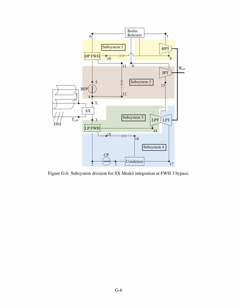
1
5
6
9
10
14
12
13
17
BFP
CP
4
3
1516
LPT
2
HP FWH
LP FWH
LPT
IPT
HPT
Condenser
7
8
11
SX
BoilerReheater
Wnet
3s
T s,o
ut
Ts,in
Subsystem 4
Subsystem 3
Subsystem 2
Subsystem 1
DNI
Figure G.6: Subsystem division for SX Model integration at FWH 3 bypass.
G-6

1
5
6
9
10
14
12
13
17
BFP
CP
4
3
1516
LPT
2
HP FWH
LP FWH
LPT
IPT
HPT
Condenser
7
8
11
BoilerReheater
Wnet5s
T s,o
ut
Ts,in
SX
Subsystem 4
Subsystem 3
Subsystem 2
Subsystem 1
DNI
Figure G.7: Subsystem division for SX Model integration at FWH 5 or FWH 6 bypass..
G-7

1
5
6
9
10
14
12
13
17
BFP
CP
4
3
1516
LPT
2
HP FWH
LP FWH
LPT
IPT
HPT
Condenser
7
8
11
SX
BoilerReheater
Wnet
6sT s,o
ut
Ts,in
Subsystem 4
Subsystem 3
Subsystem 2
Subsystem 1
DNI
Figure G.8: Subsystem division for SX Model integration at FWH 7 bypass.
G-8

H MATLAB Functions
H.1 Optimization
1 % SX opt
2 % Created by Aaron Bame ([email protected])
3 % v1−Initial creation.
4
5 FWHres=zeros(6,2);
6 kres=zeros(6,2);
7 % lambda=
8 zeros(6,2);
9 weights=5;
10 w(1,:)=0:(1/weights):1;
11 % w(1,1)=0.5;
12 w(2,:)=1−w(1,:);
13 %% PTC
14 for i=1:2
15 for j=1:3
16 % [kres((i*j),1),FWHres((i*j),1),˜,˜]=kopt(1,i,j,w);
17 TECH=1
18 i
19 j
20 for l=1:length(w(1,:))
21 w(1,l)
22 [kres((3*(i−1)+j),l),FWHres((3*(i−1)+j),l),˜,˜]=kopt(1,i,j,w(:,l));
23 end
24 end
25 end
26
27 %% LFR
28 for i=1:2
29 i
30 for j=1:3
31 % [kres((i*j),2),FWHres((i*j),2),˜,˜]=kopt(2,i,j,w);
32 j
33 for l=1:length(w(1,:))
34 w(1,l)
35 [kres((6+(3*(i−1)+j)),l),FWHres((6+(3*(i−1)+j)),l),˜,˜]=kopt(2,i,j,w(:,l));
36 end
H-1
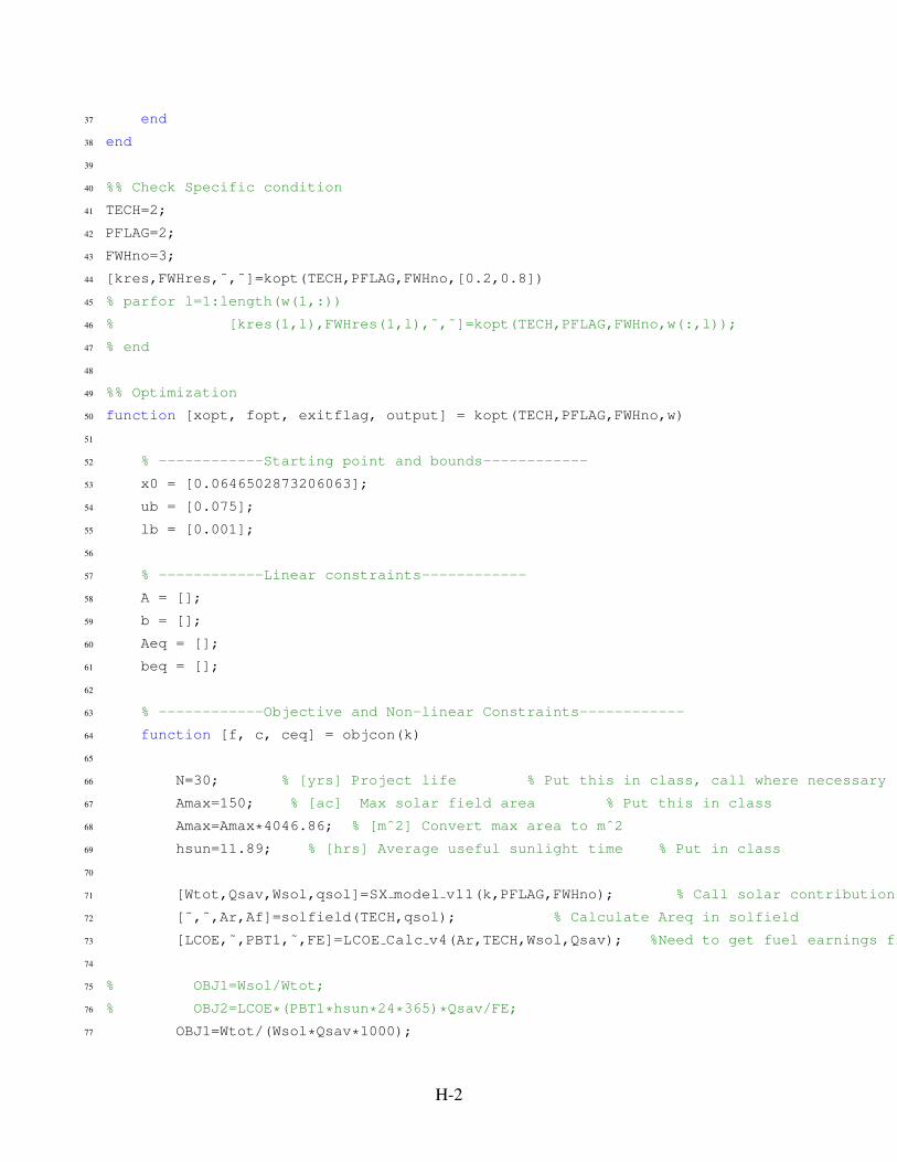
37 end
38 end
39
40 %% Check Specific condition
41 TECH=2;
42 PFLAG=2;
43 FWHno=3;
44 [kres,FWHres,˜,˜]=kopt(TECH,PFLAG,FWHno,[0.2,0.8])
45 % parfor l=1:length(w(1,:))
46 % [kres(1,l),FWHres(1,l),˜,˜]=kopt(TECH,PFLAG,FWHno,w(:,l));
47 % end
48
49 %% Optimization
50 function [xopt, fopt, exitflag, output] = kopt(TECH,PFLAG,FWHno,w)
51
52 % −−−−−−−−−−−−Starting point and bounds−−−−−−−−−−−−
53 x0 = [0.0646502873206063];
54 ub = [0.075];
55 lb = [0.001];
56
57 % −−−−−−−−−−−−Linear constraints−−−−−−−−−−−−
58 A = [];
59 b = [];
60 Aeq = [];
61 beq = [];
62
63 % −−−−−−−−−−−−Objective and Non−linear Constraints−−−−−−−−−−−−
64 function [f, c, ceq] = objcon(k)
65
66 N=30; % [yrs] Project life % Put this in class, call where necessary
67 Amax=150; % [ac] Max solar field area % Put this in class
68 Amax=Amax*4046.86; % [mˆ2] Convert max area to mˆ2
69 hsun=11.89; % [hrs] Average useful sunlight time % Put in class
70
71 [Wtot,Qsav,Wsol,qsol]=SX model v11(k,PFLAG,FWHno); % Call solar contribution from SX model
72 [˜,˜,Ar,Af]=solfield(TECH,qsol); % Calculate Areq in solfield
73 [LCOE,˜,PBT1,˜,FE]=LCOE Calc v4(Ar,TECH,Wsol,Qsav); %Need to get fuel earnings from LCOE calculations
74
75 % OBJ1=Wsol/Wtot;
76 % OBJ2=LCOE*(PBT1*hsun*24*365)*Qsav/FE;
77 OBJ1=Wtot/(Wsol*Qsav*1000);
H-2

78 OBJ2=LCOE*(PBT1*hsun*365)/FE*1e4;
79 f=w(1)*OBJ1+w(2)*OBJ2;
80
81 c=zeros(2,1);
82 c(1)=(Af−Amax)*1e−6;
83 c(2)=(PBT1−N)*1e−2;
84
85 ceq=[];
86
87 end
88
89 % −−−−−−−−−−−−Call fmincon−−−−−−−−−−−−
90 options = optimoptions(@fmincon, 'display', 'iter−detailed');
91 [xopt, fopt, exitflag, output] = fmincon(@obj, x0, A, b, Aeq, beq, lb, ub, @con, options);
92
93
94 % −−−−−−−−−−−−Separate obj/con (do not change)−−−−−−−−−−−−
95 function [f] = obj(x)
96 [f, ˜, ˜] = objcon(x);
97 end
98 function [c, ceq] = con(x)
99 [˜, c, ceq] = objcon(x);
100 end
101 % lambout=lambda.ineqlin';
102 end
H-3
H.2 Solar Integration
1 % Script to test solar exchange
2 % v1: 8/13/2019 Aaron Bame ([email protected])
3 % v2: 12/16/2019 Aaron Bame
4 % Still LPT only
5 % Add pressure ratios from Hunter data (see FWHdata.m)
6 % v3: 1/7/2020 Aaron Bame
7 % Add correlations for boiler temperature, H/IPT pressure ratios
8 % Change file date format to MM.dd.yy
9 % Add boiler outlet and HP FWH throttling valves, update numbering
10 % v4: 1/10/2020 Aaron Bame
11 % Retry constraining power with constant pressure ratios
12 % Corrected y calculation using P(8)
13 % Works well with constant pressure ratios
14 % Updated pressure ratios from FWHdata.m performs better, Qb still high
15 % v5: 4/10/2020 Aaron Bame
16 % Incorporate updated data from FWHdata.m
17 % Include correlation for boiler inlet mass flow
18 % v6: 4/21/2020 Aaron Bame
19 % Include option for HP FWH bypass
20 % Assume constant mass extraction fractions (BAD ASSUMPTION)
21 % v7: 5/16/2020 Aaron Bame
22 % Define mass fractions as constant ratio of the difference between
23 % boiler inlet and DA inlet (HP FWH) and constant fraction of LPT inlet
24 % for LP FWH.
25 % Add correlations for DA inlet flow and boiler inlet pressure
26 % v8: 6/16/2020 Aaron Bame
27 % HP FWH violates conservation of energy. h10 too low. Try moving HP FWH
28 % extraction to IPT extraction at mass averaged pressure.
29 % FWH exits should both exit at the extraction pressure and then throttle
30 % because the same temperature at lower pressure means higher
31 % enthalpy and
32 % v9: 11/6/2020 Aaron Bame
33 % Re−make function for optimization
34 % Use Correlations class
35 % v10: 11/6/2020 Aaron Bame
36 % Set FWH performance to be eta=99%
37 % v11: 11/9/2020 Aaron Bame
38 % Add constraint that the condensate water doesn't boil
H-4

39 function [Wnet,Qsav,Wsol,qs]=SX model v11(k,PFLAG,FWHno)
40
41
42 %% Power Plant Input Parameters
43 %Working fluid
44 flname='water';
45
46 % % Solar Exchange flag
47 % % SX='LP'; %LP = LP FWH Exchange
48 % SX='HP'; %HP = HP FWH Exchange
49 % % SX='SH'; %SH = Superheating after Boiler
50
51 switch PFLAG
52 case 1
53 SX='LP';
54 case 2
55 SX='HP';
56 otherwise
57 SX='SH';
58 end
59
60 N=21;
61 T=zeros(1,N);
62 P=zeros(1,N);
63 h=zeros(1,N);
64 s=zeros(1,N);
65 mdot=zeros(1,N);
66 xd=zeros(1,13); %13 Devices
67
68 %%%%%%%%%%%%%%%%%%%%%%%%%%%%%%%%%%%%%%%%%%%%%%%%%%%%%%%%%%%%%%%%%%%%%%%%%%%
69 % This area needs to be before optimization so the number of FWH's at each%
70 % pressure stage is known %
71 %%%%%%%%%%%%%%%%%%%%%%%%%%%%%%%%%%%%%%%%%%%%%%%%%%%%%%%%%%%%%%%%%%%%%%%%%%%
72 TmaxK=810; %K Boiler temp in Kelvin
73 etalp=0.918187; % Efficiency of turbines
74 etaip=0.917276;
75 etahp=0.894375;
76 etaboil=0.8978694531;
77 TTC LP=25/9;
78 TTC HP=0;
79 DCLP=50/9;
H-5
80 DCHP=50/9;
81 etacp=0.44;
82 etabfp=0.809;
83 Td=300; %K Dead state temperature
84 Tk=2445; %K Boiler flame temperature
85 Tsun=5800; %K Boundary temperature of the sun
86
87 Wmax=525; % MW−Maximum power output
88 HPlim=140;
89 IPlim=110;
90 LPlim=270;
91 BFPTlim=11;
92 Qrate=1273; % MW
93 Q0=1276;
94 % k=0.06; % Solar augment fraction
95 qs=k/(1−k)*Qrate; % MWth transferred to the cycle
96 qs=qs*1000; % convert to kW
97 if (strcmp(SX,'LP'))
98 qsollp=qs;
99 qsolhp=0;
100 else
101 qsollp=0;
102 qsolhp=qs;
103 end
104
105 %% Cycle Analysis
106
107 %List of states in order evaluated
108 % 7−Boiler exit
109 % 8−HPT exhaust
110 % 10−HP FWH extraction throttling
111 % 9−Reheat exit
112 % 13−IPT exhaust
113 % 14−LPT bleed exit
114 % 17−LPT exhaust
115 % 1−Condenser exit
116 % 2−CP exit
117 % 3−LP FWH cold exit
118 % 15−LP FWH hot exit
119 % 16−LP FWH drain cooler
120 % 6−HP FWH cold exit
H-6
121 % Guess 5−HP FWH cold inlet
122 % 11−HP FWH hot exit
123 % 12−HP FWH drain cooler
124 % 4−Mixing/deaerator
125 % Check 5 and iterate
126
127 FLAGpow=0;
128 Ps1=14; %Starting guess for 1st stage pressure (1875 psi)
129
130 rHPs1=2.9909; % Constant pressure ratio from HPT 1st stage to exhaust
131
132 %Mass Extraction fractions
133 mf7=0.37415;
134 mf6=0.150794;
135 mf5=0.188209;
136 mf3=0.037;
137 mf2=0.0355;
138 mf1=0.057;
139
140
141 while(˜FLAGpow)
142 corr=correlations(Ps1);
143 mflow=corr.mdot;
144 mda=corr.mda;
145 PBFP=corr.pbfp;
146 PHP=Ps1*corr.php;
147 rFWH6=corr.rf6;
148 rFWH5=corr.rf5;
149 rDA=corr.rda;
150 rFWH3=corr.rf3;
151 rFWH2=corr.rf2;
152 rFWH1=corr.rf1;
153 rIPT=corr.rip;
154 rRH=corr.rrh;
155 % etahp=eta7 corr(Ps1);
156 % eta6=eta6 corr(Ps1);
157 % eta5=eta5 corr(Ps1);
158 % etaipex=etaip corr(Ps1);
159 % etada=etada corr(Ps1);
160 % eta3=eta3 corr(Ps1);
161 % eta2=eta2 corr(Ps1);
H-7
162 % eta1=eta1 corr(Ps1);
163
164 dm=mflow−mda;
165
166 %Find new bleed values
167 % HP Stage
168 rHP=[rFWH5,rFWH6,rHPs1]; % High to low pressure extraction ratios
169 PHPex=Ps1/rHP(3);
170 PIPi=PHPex/rRH;
171 HPex=[PIPi./rHP(1:2),PHPex];
172 mHP=[mf5,mf6,mf7];
173 mHP=mHP.*dm;
174 % TDHP=[0,0,0];
175 if (strcmp(SX,'HP'))
176 HPex(FWHno)=[];
177 mHP(FWHno)=[];
178 end
179 hp ave=bleedpress(mHP,HPex);
180 hpbleed=hp ave(1);
181 pHPFWH=hp ave(2);
182 % etaip=eta solve([eta6,eta5,etaipex],[mHP(2:3),(mflow−sum(mHP))]);
183
184 mLPi=mflow−sum(mHP);
185 mDAex=dm−sum(mHP);
186
187 % LP Stage
188 rLP=[rFWH1,rFWH2,rFWH3,rDA]; % High to low pressure extraction ratios
189 PLPi=PIPi/rIPT;
190 LPTex=PLPi./rLP;
191 mLP=[mf1,mf2,mf3,mDAex];
192 mLP(1:3)=mLP(1:3).*mLPi;
193 Pmin=LPTex(1);
194 PCP=LPTex(end);
195 if (strcmp(SX,'LP'))
196 LPTex(FWHno)=[];
197 mLP(FWHno)=[];
198 end
199 % TDLP=[25/9,25/9,25/9];
200 lp ave=bleedpress(mLP,LPTex);
201 PLP bleed=lp ave(2);
202 lpbleed=lp ave(1);
H-8
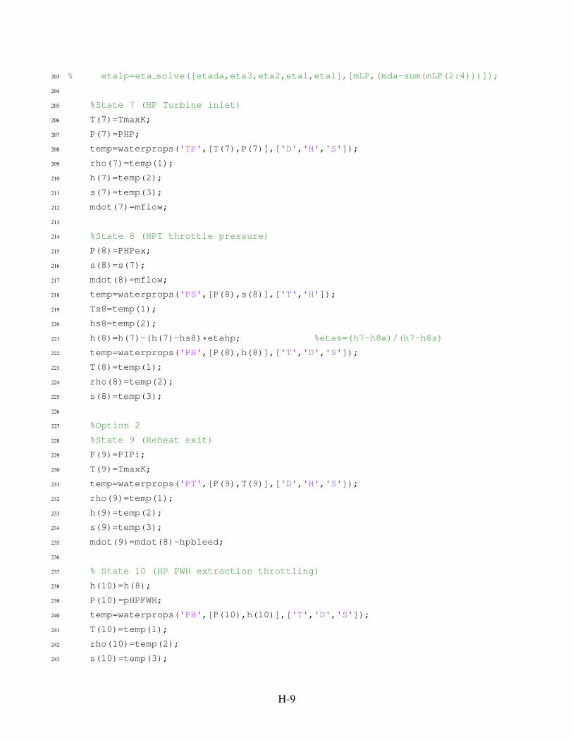
203 % etalp=eta solve([etada,eta3,eta2,eta1,eta1],[mLP,(mda−sum(mLP(2:4)))]);
204
205 %State 7 (HP Turbine inlet)
206 T(7)=TmaxK;
207 P(7)=PHP;
208 temp=waterprops('TP',[T(7),P(7)],['D','H','S']);
209 rho(7)=temp(1);
210 h(7)=temp(2);
211 s(7)=temp(3);
212 mdot(7)=mflow;
213
214 %State 8 (HPT throttle pressure)
215 P(8)=PHPex;
216 s(8)=s(7);
217 mdot(8)=mflow;
218 temp=waterprops('PS',[P(8),s(8)],['T','H']);
219 Ts8=temp(1);
220 hs8=temp(2);
221 h(8)=h(7)−(h(7)−hs8)*etahp; %etas=(h7−h8a)/(h7−h8s)
222 temp=waterprops('PH',[P(8),h(8)],['T','D','S']);
223 T(8)=temp(1);
224 rho(8)=temp(2);
225 s(8)=temp(3);
226
227 %Option 2
228 %State 9 (Reheat exit)
229 P(9)=PIPi;
230 T(9)=TmaxK;
231 temp=waterprops('PT',[P(9),T(9)],['D','H','S']);
232 rho(9)=temp(1);
233 h(9)=temp(2);
234 s(9)=temp(3);
235 mdot(9)=mdot(8)−hpbleed;
236
237 % State 10 (HP FWH extraction throttling)
238 h(10)=h(8);
239 P(10)=pHPFWH;
240 temp=waterprops('PH',[P(10),h(10)],['T','D','S']);
241 T(10)=temp(1);
242 rho(10)=temp(2);
243 s(10)=temp(3);
H-9
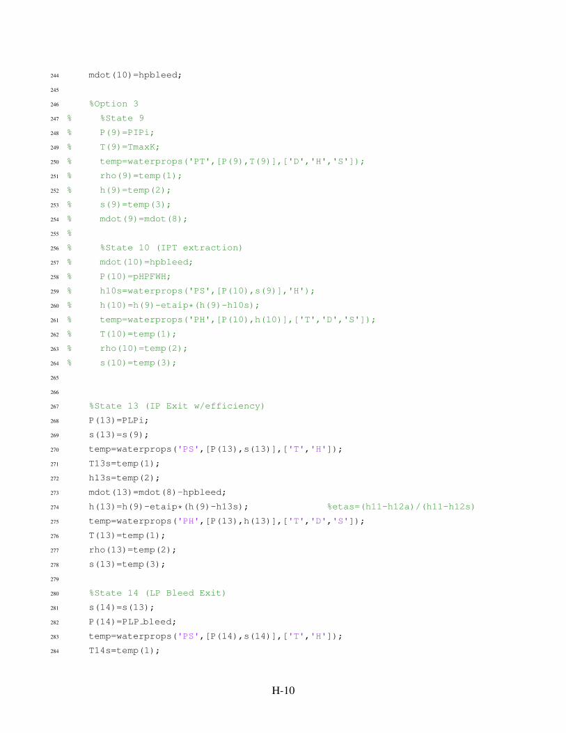
244 mdot(10)=hpbleed;
245
246 %Option 3
247 % %State 9
248 % P(9)=PIPi;
249 % T(9)=TmaxK;
250 % temp=waterprops('PT',[P(9),T(9)],['D','H','S']);
251 % rho(9)=temp(1);
252 % h(9)=temp(2);
253 % s(9)=temp(3);
254 % mdot(9)=mdot(8);
255 %
256 % %State 10 (IPT extraction)
257 % mdot(10)=hpbleed;
258 % P(10)=pHPFWH;
259 % h10s=waterprops('PS',[P(10),s(9)],'H');
260 % h(10)=h(9)−etaip*(h(9)−h10s);
261 % temp=waterprops('PH',[P(10),h(10)],['T','D','S']);
262 % T(10)=temp(1);
263 % rho(10)=temp(2);
264 % s(10)=temp(3);
265
266
267 %State 13 (IP Exit w/efficiency)
268 P(13)=PLPi;
269 s(13)=s(9);
270 temp=waterprops('PS',[P(13),s(13)],['T','H']);
271 T13s=temp(1);
272 h13s=temp(2);
273 mdot(13)=mdot(8)−hpbleed;
274 h(13)=h(9)−etaip*(h(9)−h13s); %etas=(h11−h12a)/(h11−h12s)
275 temp=waterprops('PH',[P(13),h(13)],['T','D','S']);
276 T(13)=temp(1);
277 rho(13)=temp(2);
278 s(13)=temp(3);
279
280 %State 14 (LP Bleed Exit)
281 s(14)=s(13);
282 P(14)=PLP bleed;
283 temp=waterprops('PS',[P(14),s(14)],['T','H']);
284 T14s=temp(1);
H-10
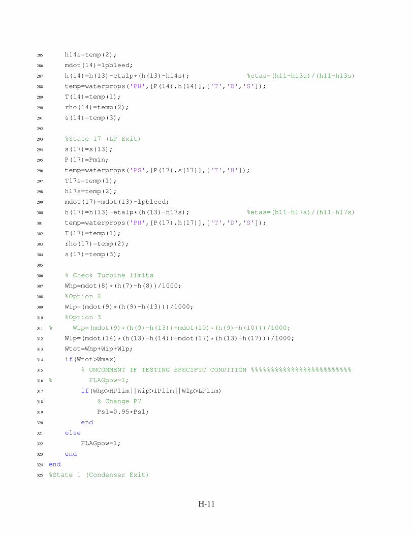
285 h14s=temp(2);
286 mdot(14)=lpbleed;
287 h(14)=h(13)−etalp*(h(13)−h14s); %etas=(h11−h13a)/(h11−h13s)
288 temp=waterprops('PH',[P(14),h(14)],['T','D','S']);
289 T(14)=temp(1);
290 rho(14)=temp(2);
291 s(14)=temp(3);
292
293 %State 17 (LP Exit)
294 s(17)=s(13);
295 P(17)=Pmin;
296 temp=waterprops('PS',[P(17),s(17)],['T','H']);
297 T17s=temp(1);
298 h17s=temp(2);
299 mdot(17)=mdot(13)−lpbleed;
300 h(17)=h(13)−etalp*(h(13)−h17s); %etas=(h11−h17a)/(h11−h17s)
301 temp=waterprops('PH',[P(17),h(17)],['T','D','S']);
302 T(17)=temp(1);
303 rho(17)=temp(2);
304 s(17)=temp(3);
305
306 % Check Turbine limits
307 Whp=mdot(8)*(h(7)−h(8))/1000;
308 %Option 2
309 Wip=(mdot(9)*(h(9)−h(13)))/1000;
310 %Option 3
311 % Wip=(mdot(9)*(h(9)−h(13))+mdot(10)*(h(9)−h(10)))/1000;
312 Wlp=(mdot(14)*(h(13)−h(14))+mdot(17)*(h(13)−h(17)))/1000;
313 Wtot=Whp+Wip+Wlp;
314 if(Wtot>Wmax)
315 % UNCOMMENT IF TESTING SPECIFIC CONDITION %%%%%%%%%%%%%%%%%%%%%%%%%
316 % FLAGpow=1;
317 if(Whp>HPlim | | Wip>IPlim | | Wlp>LPlim)318 % Change P7
319 Ps1=0.95*Ps1;
320 end
321 else
322 FLAGpow=1;
323 end
324 end
325 %State 1 (Condenser Exit)
H-11

326 P(1)=Pmin;
327 x 1=0; %Saturated liquid
328 temp=waterprops('PQ',[P(1),x 1],['T','D','H','S']);
329 T(1)=temp(1);
330 rho(1)=temp(2);
331 h(1)=temp(3);
332 s(1)=temp(4);
333 mdot(1)=lpbleed+mdot(17);
334
335 %State 2 (CP Exit)
336 s(2)=s(1);
337 P(2)=PCP;
338 mdot(2)=mdot(1);
339 temp=waterprops('PS',[P(2),s(2)],['T','H']);
340 Ts2=temp(1);
341 hs2=temp(2);
342 h(2)=h(1)+(hs2−h(1))*1/etacp; %etas=(h2s−h1)/(h2a−h1)
343 temp=waterprops('PH',[P(2),h(2)],['T','D','S']);
344 T(2)=temp(1);
345 rho(2)=temp(2);
346 s(2)=temp(3);
347
348 % State 2sol
349 P(18)=P(2);
350 mdot(18)=mdot(2);
351 if(strcmp(SX,'LP')&&(FWHno<3))
352 h(18)=qsollp/mdot(2)+h(2); %qsol=etasx*mdot(2)*(h2sol−h(2))
353 temp=waterprops('PH',[P(18),h(18)],['T','D','S']);
354 T(18)=temp(1);
355 rho(18)=temp(2);
356 s(18)=temp(3);
357 else
358 h(18)=h(2);
359 T(18)=T(2);
360 rho(18)=rho(2);
361 s(18)=s(2);
362 end
363
364 %State 15
365 mdot(15)=mdot(14);
366 P(15)=P(14);
H-12
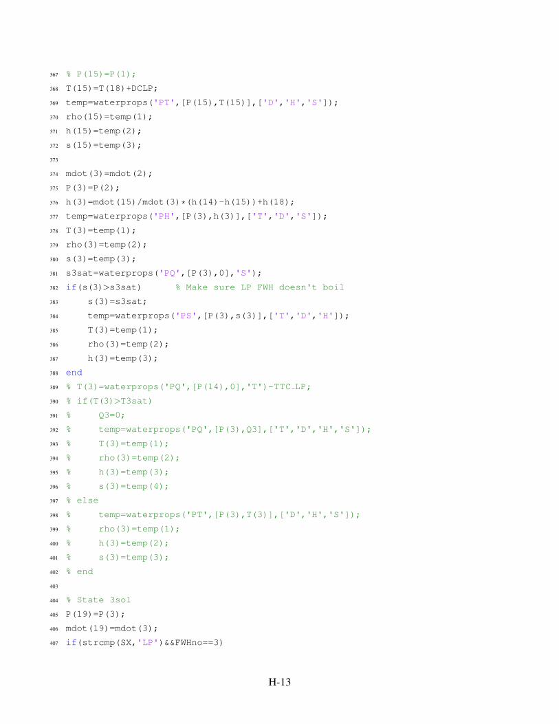
367 % P(15)=P(1);
368 T(15)=T(18)+DCLP;
369 temp=waterprops('PT',[P(15),T(15)],['D','H','S']);
370 rho(15)=temp(1);
371 h(15)=temp(2);
372 s(15)=temp(3);
373
374 mdot(3)=mdot(2);
375 P(3)=P(2);
376 h(3)=mdot(15)/mdot(3)*(h(14)−h(15))+h(18);
377 temp=waterprops('PH',[P(3),h(3)],['T','D','S']);
378 T(3)=temp(1);
379 rho(3)=temp(2);
380 s(3)=temp(3);
381 s3sat=waterprops('PQ',[P(3),0],'S');
382 if(s(3)>s3sat) % Make sure LP FWH doesn't boil
383 s(3)=s3sat;
384 temp=waterprops('PS',[P(3),s(3)],['T','D','H']);
385 T(3)=temp(1);
386 rho(3)=temp(2);
387 h(3)=temp(3);
388 end
389 % T(3)=waterprops('PQ',[P(14),0],'T')−TTC LP;
390 % if(T(3)>T3sat)
391 % Q3=0;
392 % temp=waterprops('PQ',[P(3),Q3],['T','D','H','S']);
393 % T(3)=temp(1);
394 % rho(3)=temp(2);
395 % h(3)=temp(3);
396 % s(3)=temp(4);
397 % else
398 % temp=waterprops('PT',[P(3),T(3)],['D','H','S']);
399 % rho(3)=temp(1);
400 % h(3)=temp(2);
401 % s(3)=temp(3);
402 % end
403
404 % State 3sol
405 P(19)=P(3);
406 mdot(19)=mdot(3);
407 if(strcmp(SX,'LP')&&FWHno==3)
H-13
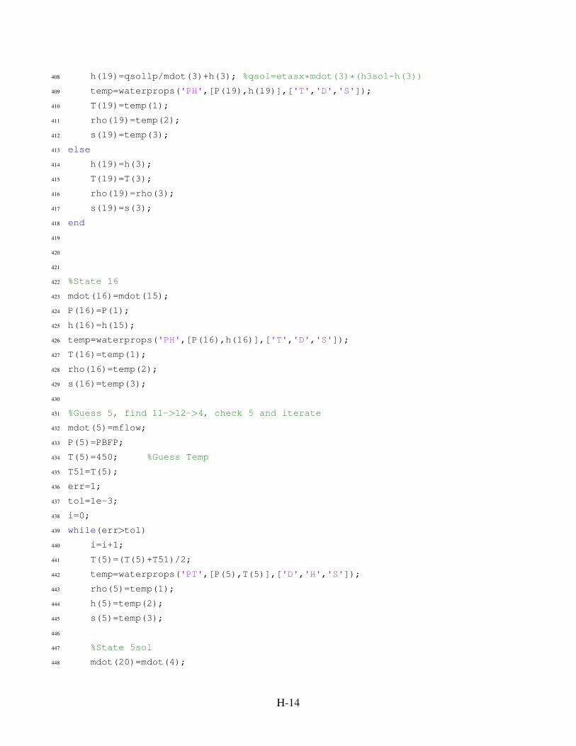
408 h(19)=qsollp/mdot(3)+h(3); %qsol=etasx*mdot(3)*(h3sol−h(3))
409 temp=waterprops('PH',[P(19),h(19)],['T','D','S']);
410 T(19)=temp(1);
411 rho(19)=temp(2);
412 s(19)=temp(3);
413 else
414 h(19)=h(3);
415 T(19)=T(3);
416 rho(19)=rho(3);
417 s(19)=s(3);
418 end
419
420
421
422 %State 16
423 mdot(16)=mdot(15);
424 P(16)=P(1);
425 h(16)=h(15);
426 temp=waterprops('PH',[P(16),h(16)],['T','D','S']);
427 T(16)=temp(1);
428 rho(16)=temp(2);
429 s(16)=temp(3);
430
431 %Guess 5, find 11−>12−>4, check 5 and iterate
432 mdot(5)=mflow;
433 P(5)=PBFP;
434 T(5)=450; %Guess Temp
435 T51=T(5);
436 err=1;
437 tol=1e−3;
438 i=0;
439 while(err>tol)
440 i=i+1;
441 T(5)=(T(5)+T51)/2;
442 temp=waterprops('PT',[P(5),T(5)],['D','H','S']);
443 rho(5)=temp(1);
444 h(5)=temp(2);
445 s(5)=temp(3);
446
447 %State 5sol
448 mdot(20)=mdot(4);
H-14

449 P(20)=P(5);
450 if(strcmp(SX,'HP')&&FWHno<3)
451 h(20)=qsolhp/mdot(5)+h(5);%qsol=mdot*(h5sol−h5)
452 temp=waterprops('PH',[P(20),h(20)],['T','D','S']);
453 T(20)=temp(1);
454 rho(20)=temp(2);
455 s(20)=temp(3);
456 else
457 h(20)=h(5);
458 T(20)=T(5);
459 rho(20)=rho(5);
460 s(20)=s(5);
461 end
462
463 %State 11
464 mdot(11)=mdot(10);
465 P(11)=P(10);
466 T(11)=T(20)+DCHP;
467 temp=waterprops('PT',[P(11),T(11)],['D','H','S']);
468 rho(11)=temp(1);
469 h(11)=temp(2);
470 s(11)=temp(3);
471
472 %State 12
473 mdot(12)=mdot(11);
474 h(12)=h(11);
475 P(12)=P(3);
476 temp=waterprops('PH',[P(12),h(12)],['T','D','S']);
477 T(12)=temp(1);
478 rho(12)=temp(2);
479 s(12)=temp(3);
480
481 %State 4
482 mdot(4)=mdot(12)+mdot(3);
483 P(4)=P(3);
484 h(4)=1/mdot(4)*(mdot(3)*h(19)+mdot(12)*h(12)); %m4*h4=m3*h3+m12*h12
485 temp=waterprops('PH',[P(4),h(4)],['T','D','S']);
486 T(4)=temp(1);
487 rho(4)=temp(2);
488 s(4)=temp(3);
489
H-15

490 %Check state 5
491 h5s=waterprops('PS',[P(5),s(4)],'H');
492 h(5)=(h5s−h(4))/etabfp+h(4); %etabfp=(h5 s−h4)/(h5−h4)
493 temp=waterprops('PH',[P(5),h(5)],['T','D','S']);
494 Tnew=temp(1);
495 rho(5)=temp(2);
496 s(5)=temp(3);
497 err=abs((T51−Tnew)/T51);
498 if(err>tol)
499 T51=Tnew;
500 else
501 T(5)=Tnew;
502 end
503 end
504
505 %State 5sol
506 mdot(20)=mdot(4);
507 P(20)=P(5);
508 if(strcmp(SX,'HP')&&FWHno<3)
509 h(20)=qsolhp/mdot(5)+h(5);%qsol=mdot*(h5sol−h5)
510 temp=waterprops('PH',[P(20),h(20)],['T','D','S']);
511 T(20)=temp(1);
512 rho(20)=temp(2);
513 s(20)=temp(3);
514 else
515 h(20)=h(5);
516 T(20)=T(5);
517 rho(20)=rho(5);
518 s(20)=s(5);
519 end
520
521 %State 6
522 mdot(6)=mflow;
523 P(6)=PBFP;
524 h(6)=mdot(10)/mdot(6)*(h(10)−h(11))+h(20);
525 temp=waterprops('PH',[P(6),h(6)],['T','D','S']);
526 T(6)=temp(1);
527 rho(6)=temp(2);
528 s(6)=temp(3);
529
530 %State 6sol
H-16
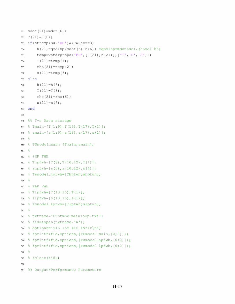
531 mdot(21)=mdot(6);
532 P(21)=P(6);
533 if(strcmp(SX,'HP')&&FWHno==3)
534 h(21)=qsolhp/mdot(6)+h(6); %qsolhp=mdot6sol*(h6sol−h6)
535 temp=waterprops('PH',[P(21),h(21)],['T','D','S']);
536 T(21)=temp(1);
537 rho(21)=temp(2);
538 s(21)=temp(3);
539 else
540 h(21)=h(6);
541 T(21)=T(6);
542 rho(21)=rho(6);
543 s(21)=s(6);
544 end
545
546 %% T−s Data storage
547 % Tmain=[T(1:9),T(13),T(17),T(1)];
548 % smain=[s(1:9),s(13),s(17),s(1)];
549 %
550 % TSmodel main=[Tmain;smain];
551 %
552 % %HP FWH
553 % Thpfwh=[T(8),T(10:12),T(4)];
554 % shpfwh=[s(8),s(10:12),s(4)];
555 % Tsmodel hpfwh=[Thpfwh;shpfwh];
556 %
557 % %LP FWH
558 % Tlpfwh=[T(13:16),T(1)];
559 % slpfwh=[s(13:16),s(1)];
560 % Tsmodel lpfwh=[Tlpfwh;slpfwh];
561 %
562 % txtname='Huntmod mainloop.txt';
563 % fid=fopen(txtname,'w');
564 % options='%16.15f %16.15f\r\n';565 % fprintf(fid,options,[TSmodel main,[0;0]]);
566 % fprintf(fid,options,[Tsmodel hpfwh,[0;0]]);
567 % fprintf(fid,options,[Tsmodel lpfwh,[0;0]]);
568 %
569 % fclose(fid);
570
571 %% Output/Performance Parameters
H-17
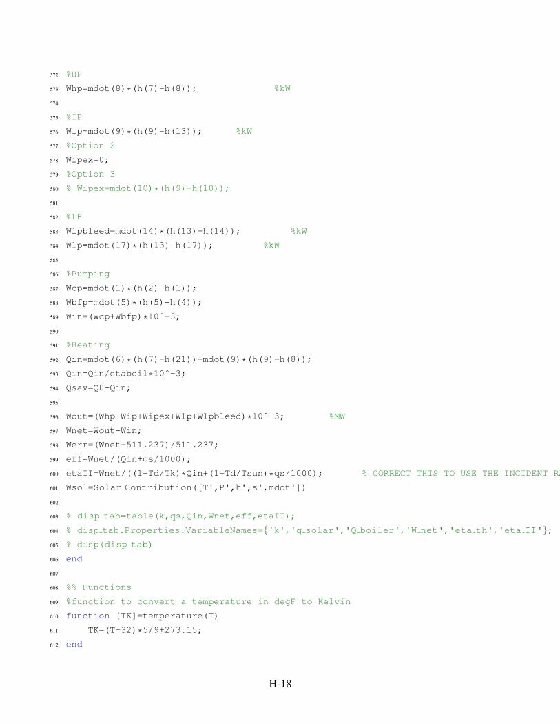
572 %HP
573 Whp=mdot(8)*(h(7)−h(8)); %kW
574
575 %IP
576 Wip=mdot(9)*(h(9)−h(13)); %kW
577 %Option 2
578 Wipex=0;
579 %Option 3
580 % Wipex=mdot(10)*(h(9)−h(10));
581
582 %LP
583 Wlpbleed=mdot(14)*(h(13)−h(14)); %kW
584 Wlp=mdot(17)*(h(13)−h(17)); %kW
585
586 %Pumping
587 Wcp=mdot(1)*(h(2)−h(1));
588 Wbfp=mdot(5)*(h(5)−h(4));
589 Win=(Wcp+Wbfp)*10ˆ−3;
590
591 %Heating
592 Qin=mdot(6)*(h(7)−h(21))+mdot(9)*(h(9)−h(8));
593 Qin=Qin/etaboil*10ˆ−3;
594 Qsav=Q0−Qin;
595
596 Wout=(Whp+Wip+Wipex+Wlp+Wlpbleed)*10ˆ−3; %MW
597 Wnet=Wout−Win;
598 Werr=(Wnet−511.237)/511.237;
599 eff=Wnet/(Qin+qs/1000);
600 etaII=Wnet/((1−Td/Tk)*Qin+(1−Td/Tsun)*qs/1000); % CORRECT THIS TO USE THE INCIDENT RADIATION, NOT JUST WHAT GOES THROUGH THE SX
601 Wsol=Solar Contribution([T',P',h',s',mdot'])
602
603 % disp tab=table(k,qs,Qin,Wnet,eff,etaII);
604 % disp tab.Properties.VariableNames={'k','q solar','Q boiler','W net','eta th','eta II'};605 % disp(disp tab)
606 end
607
608 %% Functions
609 %function to convert a temperature in degF to Kelvin
610 function [TK]=temperature(T)
611 TK=(T−32)*5/9+273.15;
612 end
H-18
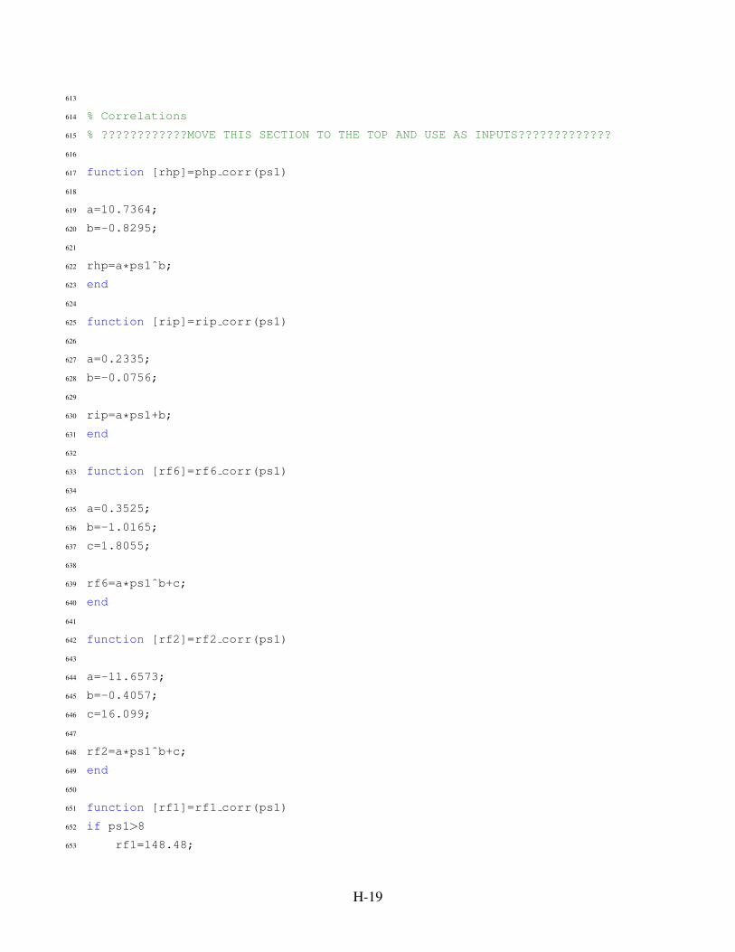
613
614 % Correlations
615 % ????????????MOVE THIS SECTION TO THE TOP AND USE AS INPUTS?????????????
616
617 function [rhp]=php corr(ps1)
618
619 a=10.7364;
620 b=−0.8295;
621
622 rhp=a*ps1ˆb;
623 end
624
625 function [rip]=rip corr(ps1)
626
627 a=0.2335;
628 b=−0.0756;
629
630 rip=a*ps1+b;
631 end
632
633 function [rf6]=rf6 corr(ps1)
634
635 a=0.3525;
636 b=−1.0165;
637 c=1.8055;
638
639 rf6=a*ps1ˆb+c;
640 end
641
642 function [rf2]=rf2 corr(ps1)
643
644 a=−11.6573;
645 b=−0.4057;
646 c=16.099;
647
648 rf2=a*ps1ˆb+c;
649 end
650
651 function [rf1]=rf1 corr(ps1)
652 if ps1>8
653 rf1=148.48;
H-19
654 else
655 a=16.8364;
656 b=−0.5346;
657
658 rf1=a*ps1+b;
659 end
660 end
661
662 function [rf3]=rf3 corr(ps1)
663
664 a=−3.7496;
665 b=−0.5717;
666 c=6.2739;
667
668 rf3=a*ps1ˆb+c;
669 end
670
671 function [mdot]=mdot corr(ps1)
672
673 a=28.977;
674 b=10.1666;
675
676 mdot=a*ps1+b;
677 end
678
679 function [mda]=mda corr(ps1)
680
681 a=25.894;
682 b=8.6345;
683
684 mda=a*ps1+b;
685 end
686
687 function [p]=pbfp corr(ps1)
688
689 a=0.9954;
690 b=0.8236;
691 c=10.8932;
692
693 p=a*ps1ˆb+c;
694 end
H-20

695
696 function [rf5]=rf5 corr(ps1)
697 a=1.5162;
698 b=−1.0184;
699 c=2.5692;
700
701 rf5=a*ps1ˆb+c;
702 end
703
704 function [rda]=rda corr(ps1)
705 a=1.3776e4;
706 b=−7.4916;
707 c=2.4598;
708
709 rda=a*ps1ˆb+c;
710 end
711
712 function [rrh]=rrh corr(ps1)
713 a=0.1011;
714 b=−1.2086;
715 c=1.07411;
716
717 rrh=a*ps1ˆb+c;
718 end
719
720 function [eta]=eta solve(etafwh,mdot)
721 mf=mdot./sum(mdot);
722 eta=sum(mf.*etafwh);
723 end
724
725 function [eta]=eta7 corr(P)
726 a=−1.2936;
727 b=−0.1537;
728 c=1.6859;
729 eta=a*Pˆb+c;
730 end
731
732 function [eta]=eta6 corr(P)
733 if(P>10)
734 eta=0.7436;
735 else
H-21

736 eta=0.7484;
737 end
738 end
739
740 function [eta]=eta5 corr(P)
741 a=−0.2603;
742 b=−0.9235;
743 c=0.9108;
744 eta=a*Pˆb+c;
745 end
746
747 function [eta]=etaip corr(P)
748 if(P>10)
749 eta=0.8689;
750 else
751 eta=0.8358;
752 end
753 end
754
755 function [eta]=etada corr(P)
756 a=−1.5309;
757 b=−2.0704;
758 c=0.5134;
759 eta=a*Pˆb+c;
760 end
761
762 function [eta]=eta3 corr(P)
763 a=0.4879;
764 b=−0.2938;
765 c=0.5004;
766 eta=a*Pˆb+c;
767 end
768
769 function [eta]=eta2 corr(P)
770 a=0.2868;
771 b=−0.3894;
772 c=0.7320;
773 eta=a*Pˆb+c;
774 end
775
776 function [eta]=eta1 corr(P)
H-22

777 a=0.3765;
778 b=0.4210;
779 c=−0.4775;
780 eta=a*Pˆb+c;
781 end
H-23

H.3 Solar Contribution
1 % Function to calculate the solar contribution of the hybrid CSP and coal
2 % power plant
3 % Created 5/13/2020 by Joseph Furner ([email protected])
4
5 % Inputs:
6 % Nodes −type: 21x5 matrix (i.e. [484.02,5.99,3135.3,2.7,470.0;460,2.5,1055.4,2.9,435.4;...])
7 % meaning: state point properties. Colums are in order from
8 % left to right: Temperature [K], pressure [MPa], enthalpy
9 % [kJ/kg], entropy [kJ/kg−K], mass flow rate [kg/s]. Rows are in
10 % order from node 1 to node 17 where the last rows are solar echange outlets.
11 % Outputs:
12 % Wsol −type: double
13 % meaning: Solar contribution [MW]
14 %
15 function [Wsol,eD,sprpo,esol] = Solar Contribution(Nodes)
16
17 state = Nodes(1:17,:);
18 sol = Nodes(18:end,:);
19
20 T0 = 298;
21 T = state(:,1);
22 P = state(:,2);
23 H = state(:,3);
24 S = state(:,4);
25 mdot = state(:,5);
26
27
28 % Subsystem 1
29 in{1} = [H(7) S(7) mdot(7);H(5) S(5) mdot(5)];
30 out{1} = [H(8) S(8) mdot(9);H(6) S(6) mdot(6);H(11) S(11) mdot(11)];
31 % Subsystem 2
32 in{2} = [H(9) S(9) mdot(9);H(3) S(3) mdot(3);H(11) S(11) mdot(11)];
33 out{2} = [H(13) S(13) mdot(13);H(5) S(5) mdot(5)];
34 % Subsystem 3
35 in{3} = [H(13) S(13) mdot(13);H(2) S(2) mdot(2)];
36 out{3} = [H(14) S(14) mdot(17);H(3) S(3) mdot(3);H(15) S(15) mdot(15)];
37 % Subsystem 4
38 in{4} = [H(14) S(14) mdot(17);H(15) S(15) mdot(15)];
H-24
39 out{4} = [H(2) S(2) mdot(2)];
40
41 if sol(1,4) ˜= S(2)
42 used = 1;
43 Hsol = [H(2) sol(1,3)];
44 Ssol = [S(2) sol(1,4)];
45 in{3}(2,1:2) = [Hsol(2) Ssol(2)];
46 msprpo = [mdot(7) mdot(9) mdot(2)];
47 elseif sol(2,4) ˜= S(3)
48 used = 2;
49 Hsol = [H(3) sol(2,3)];
50 Ssol = [S(3) sol(2,4)];
51 in{2}(2,1:2) = [Hsol(2) Ssol(2)];
52 msprpo = [mdot(7) mdot(9) mdot(3)];
53 elseif sol(3,4) ˜= S(5)
54 used = 3;
55 Hsol = [H(5) sol(3,3)];
56 Ssol = [S(5) sol(3,4)];
57 in{1}(2,1:2) = [Hsol(2) Ssol(2)];
58 msprpo = [mdot(7) mdot(9) mdot(5)];
59 elseif sol(4,4) ˜= S(6)
60 used = 4;
61 Hsol = [H(6) sol(4,3)];
62 Ssol = [S(6) sol(4,4)];
63 msprpo = [mdot(7) mdot(9) mdot(6)];
64 end
65
66 liquid = [T(2),S(2);sol(1,1),sol(1,4);T(3),S(3);sol(2,1),sol(2,4);T(4),S(4);T(5),S(5);sol(3,1),sol(3,4);T(6),S(6);sol(4,1),sol(4,4)];
67 Ssprpo = [Ssol(1) Ssol(2) sol(4,4) S(7) S(8) S(9)];
68 m0 = mdot(7);
69 Ps = P(7);
70 Prh = P(9);
71 Pw = [Ps Prh];
72 Sthtl = [S(8) S(10)];
73 Tthtl = [T(8) T(10)];
74 Pcs = [P(6) P(10) P(13) P(14) P(17)];
75 TS = zeros(1,length(Ssprpo));
76 for i = 1:length(Pcs)
77 for j = 1:length(Ssprpo)
78 TS(i,j) = waterprops('PS',[Pcs(i),Ssprpo(j)],'T');
79 % if Pcs(i) <= Psol(1)
H-25

80 % TS(i,j) = waterprops('PS',[Pcs(i),Ssprpo(j)],'T');
81 % else
82 % if j > 2
83 % TS(i,j) = waterprops('PS',[Pcs(i),Ssprpo(j)],'T');
84 % else
85 % TS(i,j) = Tsol(j);
86 % end
87 % end
88 end
89 end
90 WHPT = (H(7) − H(8))*mdot(7);
91 WIPT = (H(9) − H(13))*mdot(9);
92 WLPT1 = (H(13) − H(14))*mdot(13);
93 WLPT2 = (H(14) − H(17))*mdot(17);
94 WBFP = mdot(4)*(H(5)−H(4));
95 WCP = mdot(1)*(H(2) − H(1));
96 Qcon = (mdot(17)*H(17)) + (mdot(16)*H(16)) − (mdot(1)*H(1));
97 Xwq = [WHPT,WIPT − WBFP,WLPT1,WLPT2 + ((1 − (T0/T0))*Qcon) − WCP];
98
99
100
101 eD = zeros(1,4);
102 sprpo = zeros(1,4);
103 for i = 1:4
104 if i > 2
105 Sthtl = [0 0];
106 Tthtl = [0 0];
107 end
108 if used == 1
109 if i < 4
110 sprpo(i) = 0;
111 else
112 [sprpo(i)] = Solar Prop([Pcs(i),Pcs(i+1)],msprpo,Ssprpo,Pw,TS(i:i+1,:),Sthtl,Tthtl,liquid,[H(6),H(7)]);
113 end
114 elseif used == 2
115 if i < 3
116 sprpo(i) = 0;
117 else
118 [sprpo(i)] = Solar Prop([Pcs(i),Pcs(i+1)],msprpo,Ssprpo,Pw,TS(i:i+1,:),Sthtl,Tthtl,liquid,[H(6),H(7)]);
119 end
120 elseif used == 3
H-26
121 if i < 2
122 sprpo(i) = 0;
123 else
124 [sprpo(i)] = Solar Prop([Pcs(i),Pcs(i+1)],msprpo,Ssprpo,Pw,TS(i:i+1,:),Sthtl,Tthtl,liquid,[H(6),H(7)]);
125 end
126 elseif used == 4
127 if i < 1
128 sprpo(i) = 0;
129 else
130 [sprpo(i)] = Solar Prop([Pcs(i),Pcs(i+1)],msprpo,Ssprpo,Pw,TS(i:i+1,:),Sthtl,Tthtl,liquid,[H(6),H(7)]);
131 end
132 end
133 ein = sum((in{i}(:,1) − T0.*(in{i}(:,2))).*in{i}(:,3));134 eout = sum((out{i}(:,1) − T0.*(out{i}(:,2))).*out{i}(:,3));135 eD(i) = (ein − eout − Xwq(i))/m0;
136
137 end
138
139 esol = (msprpo(3)/m0)*((Hsol(2) − Hsol(1)) − T0*(Ssol(2) − Ssol(1)));
140 Wsol = 0.001*m0*(esol − sum(eD.*sprpo));
141 end
H-27
H.4 Solar Data
1 %% Header
2 % Created by Aaron Bame ([email protected])
3 % v1: 12/3/2019
4 % Script to scrub multiple years of solar resource data downloaded from
5 % NREL's NSRDB (https://maps.nrel.gov/nsrdb−viewer)
6
7 % Assumes downloading data for:
8 % yr | month | day | hr | min | DHI | DNI | Clearsky DNI | humid | Temp
9
10 % Currently assumes every 30 minutes
11
12 % v2: 12/6/2019−Aaron Bame
13 % Update downloaded data order:
14 % yr | month | day | hr | min | DNI | CSDNI | zenith | Temp | Pressure
15 % Calculate average daily zenith, correspondingly correct indices
16
17 %% Set up calendar array %calendar=[month; date; DNI; CSDNI; theta; Dayhrs]
18 calendar=zeros([365,6]);
19 begin=1;
20 %January (31 day)
21 jan=31;
22 calendar(begin:(begin+jan−1),1)=1;
23 calendar(begin:(begin+jan−1),2)=[1:1:jan];
24 begin=begin+jan;
25 %February(28 day)
26 feb=28;
27 calendar(begin:(begin+feb−1),1)=2;
28 calendar(begin:(begin+feb−1),2)=[1:1:feb];
29 begin=begin+feb;
30 %March (31 day)
31 mar=31;
32 calendar(begin:(begin+mar−1),1)=3;
33 calendar(begin:(begin+mar−1),2)=[1:1:mar];
34 begin=begin+mar;
35 %April (30 day)
36 apr=30;
37 calendar(begin:(begin+apr−1),1)=4;
38 calendar(begin:(begin+apr−1),2)=[1:1:apr];
H-28

39 begin=begin+apr;
40 %May (31 day)
41 may=31;
42 calendar(begin:(begin+may−1),1)=5;
43 calendar(begin:(begin+may−1),2)=[1:1:may];
44 begin=begin+may;
45 %June (30 day)
46 jun=30;
47 calendar(begin:(begin+jun−1),1)=6;
48 calendar(begin:(begin+jun−1),2)=[1:1:jun];
49 begin=begin+jun;
50 %July (31 day)
51 jul=31;
52 calendar(begin:(begin+jul−1),1)=7;
53 calendar(begin:(begin+jul−1),2)=[1:1:jul];
54 begin=begin+jul;
55 %August (31 day)
56 aug=31;
57 calendar(begin:(begin+aug−1),1)=8;
58 calendar(begin:(begin+aug−1),2)=[1:1:aug];
59 begin=begin+aug;
60 %September (30 day)
61 sep=30;
62 calendar(begin:(begin+sep−1),1)=9;
63 calendar(begin:(begin+sep−1),2)=[1:1:sep];
64 begin=begin+sep;
65 %October (31 day)
66 oct=31;
67 calendar(begin:(begin+oct−1),1)=10;
68 calendar(begin:(begin+oct−1),2)=[1:1:oct];
69 begin=begin+oct;
70 %November (30 day)
71 nov=30;
72 calendar(begin:(begin+nov−1),1)=11;
73 calendar(begin:(begin+nov−1),2)=[1:1:nov];
74 begin=begin+nov;
75 %December (31 day)
76 dec=31;
77 calendar(begin:(begin+dec−1),1)=12;
78 calendar(begin:(begin+dec−1),2)=[1:1:dec];
79 begin=begin+dec;
H-29

80
81 months=[jan,feb,mar,apr,may,jun,jul,aug,sep,oct,nov,dec];
82
83 %% Import the data
84
85 % Asks the user to select file(s)
86 % May select multiple files, must be from the same folder
87 [names,path]=uigetfile('*.csv','MultiSelect','on');
88 files=length(names);
89
90 % Repeat for each year of data
91 for i=1:files
92
93 % Combine the file path and name into a single file name
94 f=fullfile(path,names(i));
95 % Convert filename to a character variable
96 filename=char(f);
97 %Begin reading data from A4 of the .csv file
98 data=csvread(filename,3,0);
99
100 % Assign imported array to column variable names
101 year = data(:,1);
102 month = data(:,2);
103 day = data(:,3);
104 hour = data(:,4);
105 minute = data(:,5);
106 DNI = data(:,6); %W/mˆ2
107 CSDNI = data(:,7); %W/mˆ2
108 thetaz = data(:,8);
109 Temp = data(:,9);
110 Press = data(:,10);
111
112 % Clear temporary variables
113 clearvars data f;
114
115 N=48; %Number of readings in one day (Automate?)
116
117 %% Data Analysis
118 % Find the average for each day and then average across the whole month
119 for j=1:365 %Iterate through each day
120
H-30
121 begin=j*N−47;
122 midnight=j*N;
123
124 rise=find(CSDNI(begin:midnight)>0,1,'first');
125 set=find(CSDNI(begin:midnight)>0,1,'last');
126
127
128 % Daily flux average
129 a=begin+rise−1;
130 b=begin+set−1;
131 calendar(j,3)=calendar(j,3)+avg(DNI(a:b));
132 calendar(j,4)=calendar(j,4)+avg(CSDNI(a:b));
133 calendar(j,5)=calendar(j,5)+avg(thetaz(a:b));
134 calendar(j,6)=calendar(j,6)+(set−rise+1)/2;
135
136
137 end
138 end
139
140 % Calculate the average for each day
141 calendar(:,3)=calendar(:,3)/files;
142 calendar(:,4)=calendar(:,4)/files;
143 calendar(:,5)=calendar(:,5)/files;
144 calendar(:,6)=calendar(:,6)/files;
145
146 %% Data presentation
147 % Yearly average flux [W/mˆ2]
148 yearavg=sum(calendar(:,3))/length(calendar(:,3))
149 % Clear sky yearly average (Maximum solar condition) [W/mˆ2]
150 CSyearavg=sum(calendar(:,4))/length(calendar(:,4))
151 % Average hours of daylight [hrs]
152 hrs=sum(calendar(:,6))/length(calendar(:,6))
153 % Yearly average energy [kWh/mˆ2]
154 yrly energy=yearavg*hrs/1000
155
156 %% Trap Rule Integration
157 function [sum]=traps(light data)
158 N=length(light data);
159 sum=light data(1);
160 for i=2:(N−1)
161 sum=sum+2*light data(i);
H-31
162 end
163 sum=sum+light data(N);
164 sum=sum/4; % When dx=0.5 hrs, dx/2=1/4
165 end
166
167 %% Daily average
168 function [result]=avg(flux)
169 N=length(flux);
170 result=sum(flux)/N;
171 end
H-32
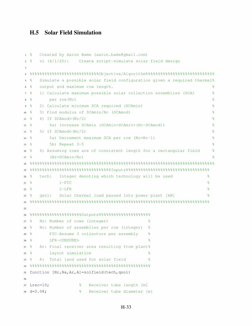
H.5 Solar Field Simulation
1 % Created by Aaron Bame ([email protected])
2 % v1 (4/1/20): Create script−simulate solar field design
3
4 %%%%%%%%%%%%%%%%%%%%%%%%%%%%Objective/Algorithm%%%%%%%%%%%%%%%%%%%%%%%%%%%%
5 % Simulate a possible solar field configuration given a required thermal%
6 % output and maximum row length. %
7 % 1) Calculate maximum possible solar collection assemblies (SCA) %
8 % per row(Nc) %
9 % 2) Calculate minimum SCA required (SCAmin) %
10 % 3) Find modulus of SCAmin/Nc (SCAmod) %
11 % 4) If SCAmod>(Nc/2) %
12 % 4a) Increase SCAmin (SCAmin=SCAmin+(Nc−SCAmod)) %
13 % 5) If SCAmod<(Nc/2) %
14 % 5a) Decrement maximum SCA per row (Nc=Nc−1) %
15 % 5b) Repeat 3−5 %
16 % 6) Assuming rows are of consistent length for a rectangular field %
17 % (Nr=SCAmin/Nc) %
18 %%%%%%%%%%%%%%%%%%%%%%%%%%%%%%%%%%%%%%%%%%%%%%%%%%%%%%%%%%%%%%%%%%%%%%%%%%%
19 %%%%%%%%%%%%%%%%%%%%%%%%%%%%%%%%%Inputs%%%%%%%%%%%%%%%%%%%%%%%%%%%%%%%%%%
20 % tech: Integer denoting which technology will be used %
21 % 1−PTC %
22 % 2−LFR %
23 % qsol: Solar thermal load passed into power plant [kW] %
24 %%%%%%%%%%%%%%%%%%%%%%%%%%%%%%%%%%%%%%%%%%%%%%%%%%%%%%%%%%%%%%%%%%%%%%%%%
25
26 %%%%%%%%%%%%%%%%%%%%%Outputs%%%%%%%%%%%%%%%%%%%%%
27 % Nr: Number of rows (integer) %
28 % Nc: Number of assemblies per row (integer) %
29 % PTC−Assume 3 collectors per assembly %
30 % LFR−<UNSURE> %
31 % Ar: Final receiver area resulting from plant%
32 % layout simulation %
33 % A: Total land used for solar field %
34 %%%%%%%%%%%%%%%%%%%%%%%%%%%%%%%%%%%%%%%%%%%%%%%%%
35 function [Nr,Na,Ar,A]=solfield(tech,qsol)
36
37 Lrec=10; % Receiver tube length [m]
38 d=0.08; % Receiver tube diameter [m]
H-33
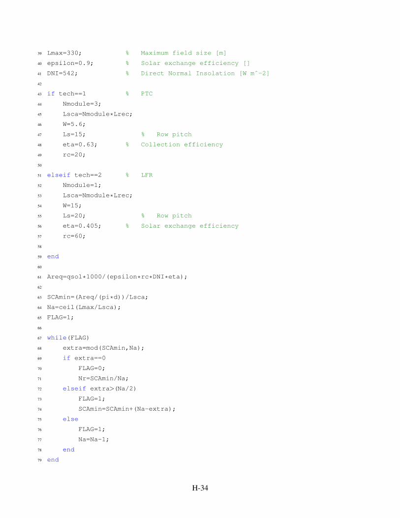
39 Lmax=330; % Maximum field size [m]
40 epsilon=0.9; % Solar exchange efficiency []
41 DNI=542; % Direct Normal Insolation [W mˆ−2]
42
43 if tech==1 % PTC
44 Nmodule=3;
45 Lsca=Nmodule*Lrec;
46 W=5.6;
47 Ls=15; % Row pitch
48 eta=0.63; % Collection efficiency
49 rc=20;
50
51 elseif tech==2 % LFR
52 Nmodule=1;
53 Lsca=Nmodule*Lrec;
54 W=15;
55 Ls=20; % Row pitch
56 eta=0.405; % Solar exchange efficiency
57 rc=60;
58
59 end
60
61 Areq=qsol*1000/(epsilon*rc*DNI*eta);
62
63 SCAmin=(Areq/(pi*d))/Lsca;
64 Na=ceil(Lmax/Lsca);
65 FLAG=1;
66
67 while(FLAG)
68 extra=mod(SCAmin,Na);
69 if extra==0
70 FLAG=0;
71 Nr=SCAmin/Na;
72 elseif extra>(Na/2)
73 FLAG=1;
74 SCAmin=SCAmin+(Na−extra);
75 else
76 FLAG=1;
77 Na=Na−1;
78 end
79 end
H-34

80
81 A=(Na*Nmodule*Lrec)*(W*Nr+(Ls−W)*(Nr−1));
82 Ar=pi*d*Lsca*Nr*Na;
83
84 % N=[Nr,Na,Ar,A];
85
86 end
H-35

H.6 Financial Model
1 function [LCOE,CC,PBT1,PBT2,FE]= LCOE Calc v4(Ar,tech,Wsol,Esav)
2
3 %===============================BEGIN−HEADER===============================
4 % FILE: LCOE Calc.m
5 % AUTHOR: Joseph Furner
6 % DATE: 5/20/2019
7 %
8 % PURPOSE: Calculate the LCOE of a hybrid CSP and coal plant.
9 %
10 %
11 % INPUTS:
12 % Ar −type: double (i.e. 900.0)
13 % meaning: Total heat absorbtion area of the reciever tubes [m2]
14 % tech −type: index (i.e. 1)
15 % meaning: Indicates the technology type,
16 % 1 = parabolic trough,
17 % 2 = linear fresnel
18 % Wsol −type: double(i.e. 18.05)
19 % meaning: Solar contribution [MW]
20 % Esav −type: double(i.e. 220.1)
21 % meaning: Energy reduction beeing transferred into the boiler [MW]
22 %
23 %
24 % OUTPUT:
25 % LCOE −type: double (i.e. 0.001)
26 % meaning: Real Levelized Cost of Electricity [USD/kWh]
27 % CC −type: double (i.e. 60000000)
28 % meaning: Total capital cost for solar portion of project [USD]
29 % PBT1 −type: double (i.e. 10.5)
30 % meaning: Time required for cumulative cash flow to equal zero [yrs]. If PBT1 is
31 % greater than 50 years, the function will return 50.
32 % PBT2 −type: double (i.e. 10.5)
33 % meaning: Time required for cumulative fuel savings to equal the
34 % investment cost [yrs]
35 % FE −type: double (i.e. 1000000)
36 % meaning: Total amount saved from fuel savings after 50 years [USD]
37 %
38 % NOTES:
H-36
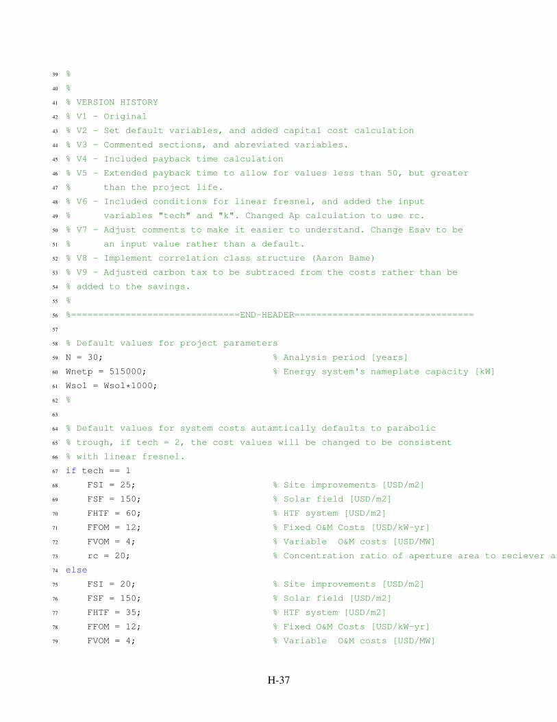
39 %
40 %
41 % VERSION HISTORY
42 % V1 − Original
43 % V2 − Set default variables, and added capital cost calculation
44 % V3 − Commented sections, and abreviated variables.
45 % V4 − Included payback time calculation
46 % V5 − Extended payback time to allow for values less than 50, but greater
47 % than the project life.
48 % V6 − Included conditions for linear fresnel, and added the input
49 % variables "tech" and "k". Changed Ap calculation to use rc.
50 % V7 − Adjust comments to make it easier to understand. Change Esav to be
51 % an input value rather than a default.
52 % V8 − Implement correlation class structure (Aaron Bame)
53 % V9 − Adjusted carbon tax to be subtraced from the costs rather than be
54 % added to the savings.
55 %
56 %===============================END−HEADER=================================
57
58 % Default values for project parameters
59 N = 30; % Analysis period [years]
60 Wnetp = 515000; % Energy system's nameplate capacity [kW]
61 Wsol = Wsol*1000;
62 %
63
64 % Default values for system costs autamtically defaults to parabolic
65 % trough, if tech = 2, the cost values will be changed to be consistent
66 % with linear fresnel.
67 if tech == 1
68 FSI = 25; % Site improvements [USD/m2]
69 FSF = 150; % Solar field [USD/m2]
70 FHTF = 60; % HTF system [USD/m2]
71 FFOM = 12; % Fixed O&M Costs [USD/kW−yr]
72 FVOM = 4; % Variable O&M costs [USD/MW]
73 rc = 20; % Concentration ratio of aperture area to reciever area
74 else
75 FSI = 20; % Site improvements [USD/m2]
76 FSF = 150; % Solar field [USD/m2]
77 FHTF = 35; % HTF system [USD/m2]
78 FFOM = 12; % Fixed O&M Costs [USD/kW−yr]
79 FVOM = 4; % Variable O&M costs [USD/MW]
H-37
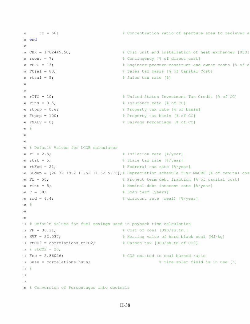
80 rc = 60; % Concentration ratio of aperture area to reciever area
81 end
82
83 CHX = 1782445.50; % Cost unit and installation of heat exchanger [USD]
84 rcont = 7; % Contingency [% of direct cost]
85 rEPC = 13; % Engineer−procure−construct and owner costs [% of direct cost]
86 Ftsal = 80; % Sales tax basis [% of Capital Cost]
87 rtsal = 5; % Sales tax rate [%]
88
89
90 rITC = 10; % United States Investment Tax Credit [% of CC]
91 rins = 0.5; % Insurance rate [% of CC]
92 rtprp = 0.6; % Property tax rate [% of basis]
93 Ftprp = 100; % Property tax basis [% of CC]
94 rSALV = 0; % Salvage Percentage [% of CC]
95 %
96
97
98 % Default Values for LCOE calculator
99 ri = 2.5; % Inflation rate [%/year]
100 rtst = 5; % State tax rate [%/year]
101 rtFed = 21; % Fedreral tax rate [%/year]
102 SCdep = [20 32 19.2 11.52 11.52 5.76];% Depreciation schedule 5−yr MACRS [% of capital cost]
103 FL = 50; % Project term debt fraction [% of capital cost]
104 rint = 5; % Nominal debt interest rate [%/year]
105 P = 30; % Loan term [years]
106 rrd = 6.4; % discount rate (real) [%/year]
107 %
108
109
110 % Default Values for fuel savings used in payback time calculation
111 FF = 36.31; % Cost of coal [USD/sh.tn.]
112 HVF = 22.037; % Heating value of hard black coal [MJ/kg]
113 rtCO2 = correlations.rtCO2; % Carbon tax [USD/sh.tn.of CO2]
114 % rtCO2 = 20;
115 Fcc = 2.86026; % CO2 emitted to coal burned ratio
116 Suse = correlations.hsun; % Time solar field is in use [h]
117 %
118
119
120 % Conversion of Percentages into decimals
H-38

121 rcont = rcont/100;
122 rEPC = rEPC/100;
123 Ftsal = Ftsal/100;
124 rtsal = rtsal/100;
125 rITC = rITC/100;
126 ri = ri/100;
127 rtst = rtst/100;
128 rtFed = rtFed/100;
129 SCdep = SCdep./100;
130 FL = FL/100;
131 rint = rint/100;
132 rins = rins/100;
133 rtprp = rtprp/100;
134 Ftprp = Ftprp/100;
135 rSALV = rSALV/100;
136 rrd = rrd/100;
137 %
138
139
140 % Calculation of nominal discount rate
141 rnomd = ((ri + 1)*(rrd + 1) − 1);
142 %
143
144
145
146
147 % Calculation of Aperture Area
148 Ap = Ar*rc;
149 %
150
151
152 % Capital cost calculation
153 % Calculate Direct Capital Cost
154 Subtotal = (FSI*Ap) + (FSF*Ap) + (FHTF*Ap) + CHX;
155 CDC = Subtotal*(1 + rcont);
156 %
157
158
159 % Calculate Indirect Capital Cost
160 CIC = (rEPC*CDC) + (Ftsal*rtsal*CDC);
161 %
H-39
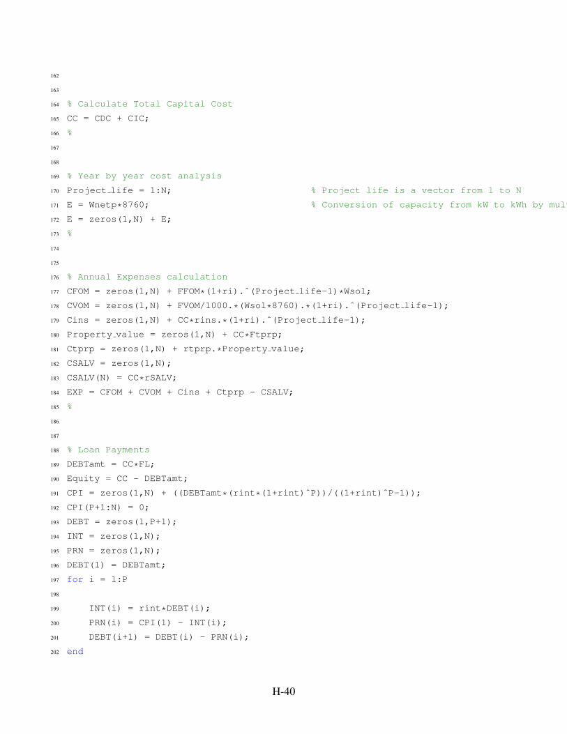
162
163
164 % Calculate Total Capital Cost
165 CC = CDC + CIC;
166 %
167
168
169 % Year by year cost analysis
170 Project life = 1:N; % Project life is a vector from 1 to N
171 E = Wnetp*8760; % Conversion of capacity from kW to kWh by multiplying by 8760 [h/yr].
172 E = zeros(1,N) + E;
173 %
174
175
176 % Annual Expenses calculation
177 CFOM = zeros(1,N) + FFOM*(1+ri).ˆ(Project life−1)*Wsol;
178 CVOM = zeros(1,N) + FVOM/1000.*(Wsol*8760).*(1+ri).ˆ(Project life−1);
179 Cins = zeros(1,N) + CC*rins.*(1+ri).ˆ(Project life−1);
180 Property value = zeros(1,N) + CC*Ftprp;
181 Ctprp = zeros(1,N) + rtprp.*Property value;
182 CSALV = zeros(1,N);
183 CSALV(N) = CC*rSALV;
184 EXP = CFOM + CVOM + Cins + Ctprp − CSALV;
185 %
186
187
188 % Loan Payments
189 DEBTamt = CC*FL;
190 Equity = CC − DEBTamt;
191 CPI = zeros(1,N) + ((DEBTamt*(rint*(1+rint)ˆP))/((1+rint)ˆP−1));
192 CPI(P+1:N) = 0;
193 DEBT = zeros(1,P+1);
194 INT = zeros(1,N);
195 PRN = zeros(1,N);
196 DEBT(1) = DEBTamt;
197 for i = 1:P
198
199 INT(i) = rint*DEBT(i);
200 PRN(i) = CPI(1) − INT(i);
201 DEBT(i+1) = DEBT(i) − PRN(i);
202 end
H-40

203 Pretax cashflow = −(CPI + EXP);
204 %
205
206
207 % State income tax
208 taxable income = zeros(1,N);
209 ITCbas = CC;
210 DEPbas = ITCbas − 0.5*(rITC*CC);
211 STATE DEP = zeros(1,N);
212 STATE DEP(1:length(SCdep)) = (SCdep*DEPbas);
213 STATE total Deductions = EXP + INT + STATE DEP;
214 STATE without deductions = taxable income−STATE total Deductions;
215 STATE = rtst*STATE without deductions;
216 STATEsav = 0 − STATE;
217 %
218
219
220 % Fedreral income tax
221 DEPbas = ITCbas − 0.5*(rITC*CC);
222 FED DEP = zeros(1,N);
223 FED DEP(1:length(SCdep)) = (SCdep*DEPbas);
224 FED total Deductions = EXP + INT + FED DEP + STATE;
225 FED without deductions = taxable income−FED total Deductions;
226 FED = rtFed*FED without deductions;
227 FED ITC = rITC*ITCbas;
228 FEDsav = 0 − FED;
229 FEDsav(1) = 0 + (FED ITC) − FED(1);
230 %
231
232 % Fuel savings and carbon tax calculation
233 FF = FF/977.4216; % Conversion from USD/sh.tn. to USD/kg
234 HVF = HVF/3.6; % Conversion from MJ/kg to kWh/kg
235 Esav = Esav*1000*Suse*365; % Conversion from MW to kWh. 365 days/yr
236 rtCO2 = rtCO2*Fcc; % Conversion from USD/sh.tn.CO2 to USD/sh.tn coal
237 rtCO2 = rtCO2/977.4216; % Conversion from USD/sh.tn to USD/kg
238 FS = FF*Esav/HVF; % Calculates fuel savings [USD]
239 TAX = rtst+rtFed*(1−rtst); % Calculates effective tax rate
240 CO2TAXsav = (rtCO2*Esav/HVF)*(1−TAX);
241 %
242
243 % Calculation of after tax costs
H-41
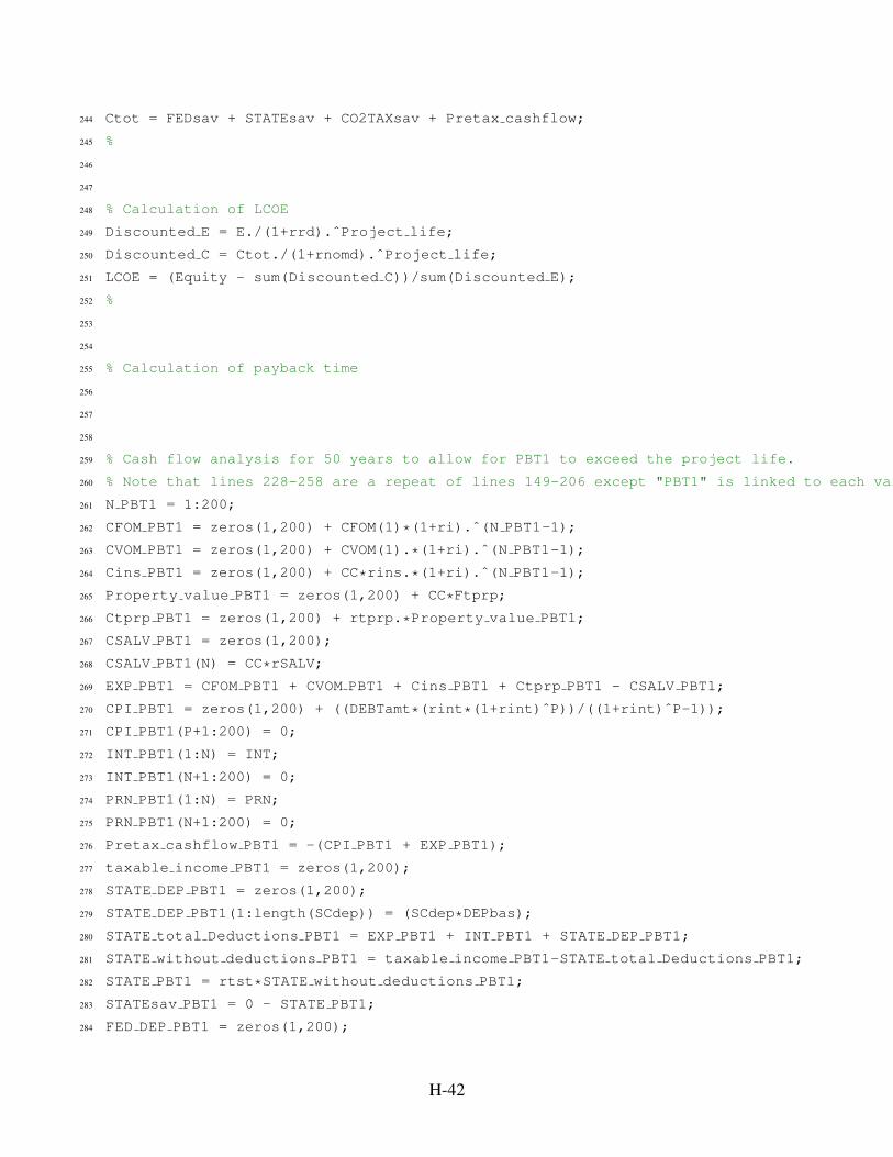
244 Ctot = FEDsav + STATEsav + CO2TAXsav + Pretax cashflow;
245 %
246
247
248 % Calculation of LCOE
249 Discounted E = E./(1+rrd).ˆProject life;
250 Discounted C = Ctot./(1+rnomd).ˆProject life;
251 LCOE = (Equity − sum(Discounted C))/sum(Discounted E);
252 %
253
254
255 % Calculation of payback time
256
257
258
259 % Cash flow analysis for 50 years to allow for PBT1 to exceed the project life.
260 % Note that lines 228−258 are a repeat of lines 149−206 except "PBT1" is linked to each variable
261 N PBT1 = 1:200;
262 CFOM PBT1 = zeros(1,200) + CFOM(1)*(1+ri).ˆ(N PBT1−1);
263 CVOM PBT1 = zeros(1,200) + CVOM(1).*(1+ri).ˆ(N PBT1−1);
264 Cins PBT1 = zeros(1,200) + CC*rins.*(1+ri).ˆ(N PBT1−1);
265 Property value PBT1 = zeros(1,200) + CC*Ftprp;
266 Ctprp PBT1 = zeros(1,200) + rtprp.*Property value PBT1;
267 CSALV PBT1 = zeros(1,200);
268 CSALV PBT1(N) = CC*rSALV;
269 EXP PBT1 = CFOM PBT1 + CVOM PBT1 + Cins PBT1 + Ctprp PBT1 − CSALV PBT1;
270 CPI PBT1 = zeros(1,200) + ((DEBTamt*(rint*(1+rint)ˆP))/((1+rint)ˆP−1));
271 CPI PBT1(P+1:200) = 0;
272 INT PBT1(1:N) = INT;
273 INT PBT1(N+1:200) = 0;
274 PRN PBT1(1:N) = PRN;
275 PRN PBT1(N+1:200) = 0;
276 Pretax cashflow PBT1 = −(CPI PBT1 + EXP PBT1);
277 taxable income PBT1 = zeros(1,200);
278 STATE DEP PBT1 = zeros(1,200);
279 STATE DEP PBT1(1:length(SCdep)) = (SCdep*DEPbas);
280 STATE total Deductions PBT1 = EXP PBT1 + INT PBT1 + STATE DEP PBT1;
281 STATE without deductions PBT1 = taxable income PBT1−STATE total Deductions PBT1;
282 STATE PBT1 = rtst*STATE without deductions PBT1;
283 STATEsav PBT1 = 0 − STATE PBT1;
284 FED DEP PBT1 = zeros(1,200);
H-42
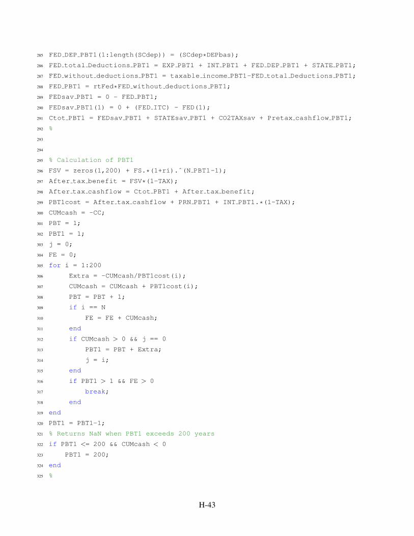
285 FED DEP PBT1(1:length(SCdep)) = (SCdep*DEPbas);
286 FED total Deductions PBT1 = EXP PBT1 + INT PBT1 + FED DEP PBT1 + STATE PBT1;
287 FED without deductions PBT1 = taxable income PBT1−FED total Deductions PBT1;
288 FED PBT1 = rtFed*FED without deductions PBT1;
289 FEDsav PBT1 = 0 − FED PBT1;
290 FEDsav PBT1(1) = 0 + (FED ITC) − FED(1);
291 Ctot PBT1 = FEDsav PBT1 + STATEsav PBT1 + CO2TAXsav + Pretax cashflow PBT1;
292 %
293
294
295 % Calculation of PBT1
296 FSV = zeros(1,200) + FS.*(1+ri).ˆ(N PBT1−1);
297 After tax benefit = FSV*(1−TAX);
298 After tax cashflow = Ctot PBT1 + After tax benefit;
299 PBT1cost = After tax cashflow + PRN PBT1 + INT PBT1.*(1−TAX);
300 CUMcash = −CC;
301 PBT = 1;
302 PBT1 = 1;
303 j = 0;
304 FE = 0;
305 for i = 1:200
306 Extra = −CUMcash/PBT1cost(i);
307 CUMcash = CUMcash + PBT1cost(i);
308 PBT = PBT + 1;
309 if i == N
310 FE = FE + CUMcash;
311 end
312 if CUMcash > 0 && j == 0
313 PBT1 = PBT + Extra;
314 j = i;
315 end
316 if PBT1 > 1 && FE > 0
317 break;
318 end
319 end
320 PBT1 = PBT1−1;
321 % Returns NaN when PBT1 exceeds 200 years
322 if PBT1 <= 200 && CUMcash < 0
323 PBT1 = 200;
324 end
325 %
H-43

326
327
328 % Calculation of PBT2
329 PBT2 = log(((CC*ri)/(FS + CO2TAXsav))+1)/log(1+ri);
330 %
331
332 end
H-44