steady-state simulation of queueing processes: a survey of
TRANSCRIPT

Steady-State Simulation of Queueing Processes: A Survey of Problems and Solutions
KRZYSZTOF PAWLIKOWSKI
Department of Computer Science, University of Canterbury, Christchurch, New Zealand
For years computer-based stochastic simulation has been a commonly used tool in the performance evaluation of various systems. Unfortunately, the results of simulation studies quite often have little credibility, since they are presented without regard to their random nature and the need for proper statistical analysis of simulation output data.
This paper discusses the main factors that can affect the accuracy of stochastic simulations designed to give insight into the steady-state behavior of queuing processes. The problems of correctly starting and stopping such simulation experiments to obtain the required statistical accuracy of the results are addressed. In this survey of possible solutions, the emphasis is put on possible applications in the sequential analysis of output data, which adaptively decides about continuing a simulation experiment until the required accuracy of results is reached. A suitable solution for deciding upon the starting point of a steady-state analysis and two techniques for obtaining the final simulation results to a required level of accuracy are presented, together with pseudocode implementations.
Categories and Subject Descriptors: G.3 [Probability and Statistics]: Statistical Computing, Statistical Software; G.4 [Mathematical Software]: Efficiency, Reliability and Robustness; G.m [Miscellaneous]: Queuing Theory; 1.6.4 [Simulation and Modeling]: Model Validation and Analysis
General Terms: Algorithms, Performance, Theory
Additional Key Words and Phrases: Automation of simulation experiments, initial transient period, precision of simulation results, sequential analysis of confidence intervals, statistical analysis of simulation output data, stopping rules for steady-state simulation
INTRODUCTION
Computer-based stochastic simulation, tra- ditionally regarded as a last resort tool (if analytical methods fail), has become a valid and commonly used method of performance evaluation. This popularity is due to the continuing development of more powerful and less expensive computers, as well as significant achievements in software engi- neering. One can observe a trend toward integrating simulation methodology with
concepts and methods of artificial intelli- gence [Artificial Intelligence 19881. Various user-friendly simulation packages offer vi- sual interactive capabilities; traditional discrete-event simulation modeling is more and more frequently supported by ob- ject and logic-oriented programming and various concepts of artificial intelligence [Bell and O’Kneefe 1987; Gates et al. 1988; Jackman and Medeiros 1988; Kerckhoffs and Vansteenkiste 1986; Knapp 1986; Oren and Zeigler 1987; Reedy 1987; Ruiz-Mier
Permission to copy without fee all or part of this material is granted provided that the copies are not made or distributed for direct commercial advantage, the ACM copyright notice and the title of the publication and its date appear, and notice is given that copying is by permission of the Association for Computing Machinery. To copy otherwise, or to republish, requires a fee and/or specific permission. 0 1990 ACM 0360-0300/90/0600-0123 $01.50
ACM Computing Surveys, Vol. 22, No. 2, June 1990

124 . Krzysztof Pawlikowski
CONTENTS
INTRODUCTION 1. METHODS OF DATA COLLECTION AND
ANALYSIS 2. PROBLEM OF INITIALIZATION
2.1 Duration of the Initial Transient Period 3. SEQUENTIAL PROCEDURES FOR STEADY-
STATE SIMULATION: EXAMPLES 3.1 Detecting the Length of the Initial Transient
Period 3.2 Sequential Testing for a Required Precision of
Results 4. SUMMARY AND GENERAL COMMENTS APPENDIX A. Elementary Statistical Concepts APPENDIX B. Spectral Analysis of Variance ACKNOWLEDGMENTS REFERENCES
and Talavage 1987; Stairmand and Kreutzer 1988; Zeigler 19871. All of these developments offer users increasingly pow- erful and versatile techniques for per- formance evaluation, leading toward automatic, knowledge-based simulation packages. Simulation programming tech- niques and languages are discussed in nu- merous publications including textbooks by Bulgren [ 19821, Kreutzer [ 19861, Law and Kelton [1982a], and Payne [1982].
Applying simulation to the modeling and performance analysis of complex systems can be compared to using the surgical scal- pel [Shannon 19811, whereby “in the right hand [it] can accomplish tremendous good, but it must be used with great care and by someone who knows what they are doing.” One of the applications in which simulation has become increasingly popular is the class of dynamic systems with random input and output processes, represented for example by computer communication networks. In such cases, regardless of how advanced the programming methodology applied to sim- ulation modeling is, since simulated events are controlled by random numbers, the results produced are nothing more than statistical samples. Therefore, various sim- ulation studies, frequently reported in tech- nical literature, can be regarded as programming exercises only. The authors
of such studies, after putting much intellec- tual effort and time into building simula- tion models and then writing and running programs, have very little or no interest in a proper analysis of the simulation results. It is true that “the purpose of modeling is insight, not numbers” [Hamming 19621, but proper insight can only be obtained from correctly analyzed numbers. Other modes of presenting results, for example, animation, can be very attractive and useful when the model is validated, but nothing can substitute the need for statistical analysis of simulation output data in stud- ies aimed at performance analysis; see also Schruben [ 19871.
In the stochastic simulation of, for ex- ample, queuing systems “computer runs yield a mass of data but this mass may turn into a mess.” If the random nature of the results is ignored, “instead of an expensive simulation model, a toss of the coin had better be used” [Kleijnen, 19791. Statistical inference is an absolute necessity in any situation when the same (correct) program produces different (but correct) output data from each run. Any sequence x1, x2, . . . , x, of such output data simply consists of re- alizations of random variables X1, X2, , . . , X,. Examples illustrating this fact may be found in Kelton [ 19861, Law [ 19831, Law and Keiton [1982a], and Welch [1983, Sec. 6.11.
The simplest objective of simulation studies is the estimation of the mean CL, of an analyzed process from the sequence of collected observations 3tl, x2, . . . , x,, by calculating the average as follows:
X(n) = ,il ;. (1)
Such an average assumes a random value, which depends on the sequence of obser- vations. The accuracy with which it esti- mates an unknown parameter px can be assessed by the probability
P(]X(n)-p,]<A,)=l-(Y (2a)
or
P@?(n) - A, I /Jo 5 X(n) + A,) (2b)
=l-01,
ACM Computing Surveys, Vol. 22, No. 2, June 1990

Simulation of Queueing Processes . 125
Figure 1. PITnvl c t “-,, 1-J = 1 - 42.
where A, is the half-width of the confidence interval for the estimator and (1 - cy) is the confidence level, 0 < cy < 1. Thus, if the width 2A, of the confidence interval is found for an assumed confidence level of (1 - a) and the simulation experiment were repeated a number of times, the interval (X(n) - A,, X(n) + A,) would contain an unknown average II, in lOO( 1 - cy)% of cases and would not in lOOcu% of cases. It is well known that if observations x1, x2, . . . , x, can be regarded as realizations of indepen- dent and normally distributed random vari- ables X1, X2, . . . , X,, then
where
A, = tn-pa,z~[%)l, (3)
n {xi - X(n))” ~2E(~)l = c n(n _ 1) (4)
i=l
is the (unbiased) estimator’ of the vari- ance of X(n), and tn-1,1-,/2 is the upper (1 - a/2) critical point obtained from the t-distribution with (n - 1) degrees of free- dom. In other words, for given 1 - (~12, assuming the t-distribution for the random variable T,-, = (X(n) - pJ/G[X(n)], we get PITnpl 5 t] = 1 - CY/~ for t = tn-l,l--a,2; see Figure 1 and Appendix A. For this rea- son, tn--l,l--a,2 is also called the (1 - a/2) quantile, or percentile, of the t-distribution with (n - 1) degrees of freedom. For
’ Following standard notation, 6 means an estimator of the parameter a.
n > 30, the t-distribution can be replaced by the standard normal distribution. In that case tn-1,1-,/2 in Equation (3) should be replaced by .21--a/21 which is the upper (1 - CY/~) critical point obtained from the standard normal distribution or, equiva- lently, the (1 - 01/2) quantile of the stan- dard normal distribution; see Appendix A. Commonly used values of tn-l,l-,~2 and 21-,/Z have been tabularized and can be found in many textbooks; see, for example, Trivedi [1982, Appendix 3, and p. 4891. (Warning: The definitions used for obtain- ing tabularized values should always be checked. For example, t,,-l,l-,12 and 21-,/Z are sometimes denoted as tn-l,u,2 and z,,/~, respectively.)
Equation (3) can also be applied if the observations x1, 1c2, . . . , 3c, represent ran- dom variables that are not normally dis- tributed. That is, if the observations are realizations of independent and identically distributed (i.i.d.) random variables X,, X2, . . . , X,,, then according to the central limit theorem (see Appendix A), the distribution of the variable x(n) tends to the normal distribution as the number of collected ob- servations n increases. In practice, Equa- tion (3) gives a good approximation for n > 100. Results obtained from Equations (1) and (3) are called point and interval esti- mates, respectively. Both of them are im- portant: The former characterizes the system analyzed, and the latter states the accuracy of the obtained characteristics.
If observations lcl, x2, . . . , x, cannot be regarded as realizations of i.i.d. random
ACM Computing Surveys, Vol. 22, No. 2, June 1990

126 l Krzysztof Pawlikowski
variables, we have to consider some modi- fications to the above estimators. This raises the problem of measuring the quality of estimators. There are three common measures of estimator effectiveness:
(1) The bias, which measures the system- atic deviation of the estimator from the true value of the estimated parameter; for ex- ample, in the case of X(n),
Bias[X(n)] = E[X(n) - ~~1. (5)
(2) The uariance, which measures the mean (squared) deviation of the estimator from its mean value; that is,
a2[X(n)] = E@(n) - E[X(n)])2]. (6)
(3) The mean square error (MSE) of the estimator, defined as
MSE[X(n)] = E@?(n) - ~zl~). (7)
Note that from these definitions,
MSE[R(n)]
= {Bias[X(n)]12 + a2[X(n)]. (8)
The main analytical problem encoun- tered in the analysis of simulation results is that they are usually highly correlated and thus do not satisfy the precondition of statistical independence. If observations lcl, x2, ..-, n, represent an autocorrelated and stationary sequence of random variables Xl, x2, f. *, X,, then the variance of X(n) is given by the formula
a2[X(n)] = R(0) + 2
* ;< (1 - $W]/n, (‘) where
is the autocovariance of order k (the lag k component of the autocorrelation function (R(k))) of the sequence. The autocovari- antes defined in Equation (10) are indepen- dent of the index i because of the assumed
stationarity of the analyzed processes. Note that the variance a2[X(n)] can be reduced to R(O)/n, and consequently could be esti- mated by Equation (4), if and only if the observations are uncorrelated. Neglecting the existing statistical correlation is equiv- alent to removing all the components ex- cept R(0) from Equation (9). Such an approximation is usually unacceptable. For example, in an M/M/l queuing system with 90% utilization, the variance of the mean queue length calculated according to Equa- tion (9) is 367 times greater than that from Equation (4) [Blomqvist 19671; see Law and Kelton [1982a, p. 1461 for another ex- ample. Any variance analysis disregarding correlations among the observations would lead either to an excessively optimistic con- fidence interval for Pi, in the case of posi- tively correlated observations, or to an excessively pessimistic confidence interval for pux, in the case of negatively correlated observations; see Equation (3). A positive correlation between observations is typical in simple queuing systems without feed- back connections and is stronger for higher system utilization; see, for example, Daley [1968] for correlation analysis of the M/M/l queue.
Generally, the analysis of variance of cor- related processes, and the analysis of their autocorrelation functions in particular, is a complex statistical problem and therefore creates a major difficulty in the statistical analysis of simulation output data. In ter- minating (or finite-horizon) simulation used for studying the behavior of systems during specified intervals of time, the above problem can be overcome by making a number of independent replications of the simulation experiment. In that case the means of individual observations collected during different simulation runs can be re- garded as a sequence of independent (sec- ondary) output data, and Equation (4) can be applied. Exhaustive discussions on the statistical analysis of output data from terminating simulation can be found, for example, in Kleijnen [1979, 19871, Law [ 19801, and Law and Kelton [1982a, Sec. 8.51.
In this paper, we discuss steady-state (infinite-horizon) simulation, aimed to give insight into the behavior of queuing
ACM Computing Surveys, Vol. 22, No. 2, June 1990

Simulation of Queueing Processes l 127
processes after a long period of time. The methodology for this kind of simulation study is complicated. After launching, a queuing process is initially in a nonstation- ary phase (warm-up period). Then, if the process is stable, it moves asymptotically toward a steady state (statistical equilib- rium), although different parameters usu- ally tend to the steady state with different rates. Since observations gathered during the initial transient periods do not charac- terize the steady state, a natural idea is to discard all such observations before further analysis. This requires an estimation of the effective length of the initial transient period. Ignoring the existence of this period can lead to a significant bias of the final results. On the other hand, the removal of any observations increases the variance of estimates, which in turn can increase the value of the mean-square error [Donnelly and Shannon 1981; Fishman 1972; Turn- quist and Sussman 1977; Wilson and Prit- sker 1978a]. Thus, a decision of whether to delete or not to delete initial observations depends on the assumed criterion of good- ness of the estimators. This also affects methods used to collect observations, which are discussed in Section 1. These and other aspects of the problem of initialization are presented broadly in Section 2.
Several methods of data collection and analysis have been proposed to overcome the theoretical problems that arise from the correlated nature of observations collected during steady-state simulation. We survey these methods in Section 1. They are dis- tinguished by the way they estimate the variance of observed processes; the esti- mate is needed for determining the width of the confidence intervals. Usually, the methods impose special requirements on how the output data from simulation ex- periments should be collected and prepro- cessed, which depends on whether they attempt to weaken or even remove statis- tical dependencies among observations or take the actual correlations among obser- vations into consideration. The following methods can be distinguished:
l The method of independent replications l The method of batch means l The method of overlapping batch means
Figure 2. Valid and invalid confidence in- tervals for p, in coverage analysis (in this example the coverage equals 80%).
l The method of uncorrelated sampling l The method of regenerative cycles l The method based on spectral analysis l The method based on autoregressive
representation l The method based on standardized time
series
Various approximations assumed during statistical analysis of simulation output data may bias both point and interval es- timates. For example, the final confidence interval should theoretically contain the true value of the estimated parameter with probability (1 - CY) or, equivalently, if an experiment is repeated many times, in (1 - cr)lOO% of cases; but various difficul- ties in satisfying theoretical assumptions can cause the real rate of the confidence intervals containing the true parameter to differ significantly from (1 - CX). The ro- bustness of the above methods of data col- lection and analysis is usually measured by the coverage of confidence intervals, defined as the frequency with which the intervals (X(n) - A,, X(n) + A,) contain the true parameter pcL, at a given confidence level (1 - CY), 0 < CY < 1; see Figure 2. Thus, the coverage analysis can be applied only to systems with theoretically well-known be- havior, since the value of pX has to be known. Any analyzed method must be ap- plied in a statistically significant number of repeated simulation experiments (usu- ally 200 or more replications) to determine the fraction of experiments producing the final confidence intervals covering the true mean value of the estimated parameter.
The coverage error and its main sources were theoretically analyzed by Glynn
ACM Computing Surveys, Vol. 22, No. 2, June 1990

128 l Krzysztof Pawlikowski
[ 19821, Kang and Goldsman [1985], and Schruben [1980]. Generally, a given method of data collection and analysis can be considered as producing valid lOO(1 - a)% confidence intervals (for, say, the mean delay) if the upper bound of the confidence intervals for the coverage is at least (1 - LY). Otherwise, confidence inter- vals for the estimated parameter should be regarded as invalid and the method as in- accurate. A few additional measures for the effectiveness of methods used for data col- lection and analysis were proposed in Schruben [ 19811. The weakest point of such an approach is that there is no theoretical basis for extrapolating results found for simple, analytically tractable systems to more complex systems, which are the real subjects of simulation studies; see Fox [1978].
Some conclusions on the quality of the methods can be also obtained from the analysis of the asymptotic properties of the variance estimators ~‘[X(IZ)] used by par- ticular methods for determining the width of confidence intervals. Namely, the quality of various variance estimators can be com- pared by comparing the limit values of their bias,
Bias(G2[X(rz)])
= E{G2[W(n)] - a2[X(n)]), (11)
and variance, Var{a2[X(n)]), as the number of observations tends to infinity; that is, as n 3 ~0; see Goldsman and Meketon [1985] and Goldsman et al. [1986]. Alternatively, Schmeiser [ 19821 proposed studying the asymptotic properties of the expected val- ues and variances of the halfwidth of con- fidence intervals A, generated by a method; see also Glynn and Iglehart [1985] and Goldsman and Schruben [ 19841. Following such criteria, one can say that the method using the variance estimator with the smallest bias and smallest variance, or us- ing the estimator of the width of confidence interval having the smallest expected value and smallest variance, is (asymptotically) superior to others. Unfortunately, these cri- teria are not universal since a small bias can be accompanied by large variance or vice versa. In terms of confidence intervals,
it can mean wide and very variable confi- dence intervals giving good coverage, or, conversely, stable and narrow confidence intervals giving poor coverage.
Even if we were able to collect indepen- dent and identically distributed output data from simulation runs, we cannot be fully protected from erroneous conclusions be- cause of inherent variations of simulation output data caused by the pseudorandom nature of input data; see Pidd [1984, Sec. 8.4.21 for a more detailed discussion. Certainly, one of the most important issues of any simulation experiment is to use proper input data. In the case of queuing processes this usually means se- lecting a good generator of uniformly dis- tributed (pseudo)random numbers. The state of art in this area is summarized in Park and Miller [ 19881.
The experimental accuracy of simulation can be further improved by using variance reduction techniques (VRT) developed for reducing the variance of recorded results without affecting their mean values. Sur- veys of variance reduction techniques may be found in Bratley et al. [1983, Sec. 21, Cheng [1986], Frost et al. [1988], Kleijnen [1974, Chap. 31, Law and Kelton [1982a, Chap. 111, Nelson and Schmeiser [1986], Wilson [1983, 19841. Although all of these techniques can be applied to the method of independent replications, only some of them can be fitted into other methods of data collection and analysis. Two VRTs, known as the method of control variables (or control variates) and importance sam- pling, seem to be the most frequently advocated; see, for example, Anonuevo and Nelson [ 19861, Frost et al. [ 19881, Izydorczyk et al. [1984], Lavenberg and Welch [1981], Lavenberg et al. [1982], and Venkatraman and Wilson [1985], for dis- cussion of these methods and their appli- cations. Unfortunately, despite the fact that various VRTs have been extensively studied theoretically since the beginning of digital simulation [Harling 19581, most of them have found only limited practical ap- plication. The reason is that they can be difficult to implement in simulation studies of even moderately complex systems, since they are strongly model dependent and/or
ACM Computing Surveys, Vol. 22, No. 2, June 1990

Simulation of Queueing Processes l 129
require a substantial amount of computing resources. The simplest VRT in the context of queuing processes [Law 19751, consists of a direct estimation of the mean time in queue (without service time), since this es- timator usually has a smaller variance than (direct) estimators of the mean time in the system or the mean queue length. Next, the estimates of the latter group of parameters can be obtained indirectly by applying, for example, Little’s formula. The efficiency of this approach has been proved for G/G/c queuing systems [Carson and Law 19801. A variance reduction as high as 90% has been reported, although generally the reduction tends to 0 as the system utilization tends to 100%. Indirect estimation has been found justifiable even for more complex queuing systems, provided that the inter- arrival and waiting times are negatively correlated [Glynn and Whitt 19891. An- other VRT, for achieving more stable con- fidence ktervals by reducing the variance Var(G’[X(n)]), has been proposed by Meketon and Schmeiser [1984]. They showed that the variance reduction can be achieved by calculating estimators from overlapping subsequences of output data; see the method of overlapping batch means in Section 1.
The methods for data collection and analysis can be used either in their fixed- sample-size versions or in their sequential versions. In the former case, statistical analysis is performed once at the end of the simulation experiment when a predeter- mined number of observations, assumed to be sufficient to get results of a required accuracy, has been collected. The present survey of methods for data collection and analysis, used in steady-state simulation, focusses on their sequential versions, in which the length of simulation is increased sequentially from one checkpoint to the next until a prespecified accuracy of the point estimators is obtained. Such proce- dures, which automatically control the length of simulation experiments, are very desirable in user-friendly simulation pack- ages. Sequential statistical analysis is also more efficient, since it is usually difficult to determine a priori the length of simula- tion needed by a fixed-size procedure that
would be sufficient to obtain a required width of confidence intervals at the as- sumed level of confidence [Law and Kelton 198213, 19841.
Among the few possible criteria for stop- ping the simulation, probably the most use- ful one is based on the relative (half) width of the confidence interval at a given confi- dence level (1 - a) defined as the ratio
A, ’ = X(n)
O<c<l; (12)
c.f. Equation (2). The above ratio is also called the relative
precision of the confidence interval. The simulation experiment is stopped at the first checkpoint for which E 5 E,,,, where emax is the required limit relative precision of the results at the lOO( 1 - LY) % confidence level, 0 < E,,, < 1. Note that if
l-a!
5 P[IX(n) -P,I 5 EIXbdIl, (13)
then, for pL, # 0,
PIIX(n)-pUxI 5~I-7bdll
= PI I X(n) - wx I 5 E I X(n) - px + k II
sP[IX(n)-CL,II~IX(n)-CL,I +~li.hIl,
and, finally,
l-~%P[]X(n)-~cL,] 5tlX(n)l]
where
IX(d--rzI,c 1 (14)
I CL, I -1-c ’
I X(n) - pLx I I CL, I
(15)
is called the relative error of the confidence interval.
Sequential reasoning about the statisti- cal accuracy of results is particularly advis- able if higher precision is required. There is a danger, however, since when precision requirements are increased, the resulting confidence intervals have a greater chance of not containing the true value of param- eters (the narrower the confidence interval, the worse the coverage effect). One can also
ACM Computing Surveys, Vol. 22, No. 2, June 1990

130 l Krzysztof Pawlikowski
expect that lower coverage is more probable in the case of negatively correlated obser- vations for which it is more likely to get an underestimated value of their variance. Higher accuracy requirements can also un- acceptably lengthen simulation runs con- trolled by a sequential procedure. In this context, any variance reduction technique can be regarded as a technique for speeding up the simulation, since any decrease in the value of the variance decreases the width of the resulting confidence intervals, and a specified accuracy can be met more quickly.
The sequential approach is regarded by some as the only alternative to steady- state simulation; see Bratley et al. [1983, p. 1011. Some statisticians believe that it is possible to devise a procedure that would automatically conduct data collection and analysis using a sequential rule for assess- ing the accuracy of estimates; however, a fully acceptable solution has not yet been invented. Relatively few commercially available simulation packages offer some degree of automation of statistical analysis; c.f. Catalog of Simulation Software [ 19871. For example, sequential procedures, auto- mated to some extent and based on inde- pendent replications, regenerative, and spectral methods of data collection and analysis are implemented in Research Queuing Package (RESQ), [MacNair 1985; Sauer et al. 19841, and in its network- oriented extension Performance Evalua- tion Tool (PET) [Bharath-Kumar and Kermani 19841. A method of batch means is incorporated in SIMSCRIPT II.5 [Mills 19871 and its specialized variations such as Network II.5 and COMNET 11.5. Partial automation of data analysis is also offered in Queuing Network Analysis Package Ver- sion 2 (QNAP2) [Potier 1984, 19861.
The effectiveness of proposed methods generally depends on the level of a priori knowledge of the system’s behavior. Suc- cessful fully automated implementations have been reported only for some restricted classes of queuing processes. A fully auto- mated procedure that could be used in sto- chastic simulation studies of a broader class of systems by users having little knowledge or interest in the statistical analysis of the output data is a matter for future investi-
gation. The quality of presently known methods depends on the selection of values for the various parameters involved, which requires some knowledge of the analyzed systems’ dynamics. In Section 3 we present details of two sequential procedures for data collection and analysis that were im- plemented in simulation studies of data communication protocols reported in Asgarkhani and Pawlikowski [1989] and Pawlikowski and Asgarkhani [ 19881.
This report is not addressed to statisti- cians. We avoid the strict mathematical formulation of the problems and use basic statistical terminology. Readers are re- ferred to the references for more details.
1. METHODS OF DATA COLLECTION AND ANALYSIS
During the last 25 years of discussion on the methodology of statistical analysis of output data from steady-state simulation, initiated by Conway’s [1963] “Some Tacti- cal Problems in Digital Simulation,” a va- riety of methods for data collection and analysis has been proposed to circumvent the nonstationarity of simulated queuing processes (especially the initial nonstation- arity caused by the existence of the initial transient period) and the autocorrelation of events (correlations among collected ob- servations). As has been mentioned, these methods either try to weaken (or remove) autocorrelations among observations or to exploit the correlated nature of observa- tions in analysis of variance needed for determining confidence intervals for the estimated parameters.
In the method of replications, adopted from terminating simulation, the problem with the autocorrelated nature of the orig- inal output data is overcome in a concep- tually simple way: The simulation is repeated a number of times, each time using a different, independent sequence of ran- dom numbers, and the mean value of ob- servations collected during each run is computed. These means are used in further statistical analysis as secondary, evidently independent and identically distributed output data. By the central limit theorem (see Appendix A), such data also become
ACM Computing Surveys, Vol. 22, No. 2, June 1990

Simulation of Queueing Processes l 131
approximately normally distributed. Fol- lowing these motivations, if m observations are collected during each replication, the sequence of n primary observations from kb = n/m replications (xii, 3~~2, . . . , x&, (x21, x22, . . . , X2m), . . . , bkbl, Xkb2, . . . , Xk,m)
is replaced by the sequence of their means Xl(m), X2(m), . . . , Xk,(m), where
Xi(m) = i jil xij, (16)
which are used to obtain the point and interval estimates of the process. Namely, adopting Equations (l)-(4), we get the es- timator of the mean pcL, as
Z(kb, m) = 6 ,g Xi(m), (17) b& 1
which for n = kbm is numerically equivalent to x(n). We also set the lOO(1 - a)‘% confidence interval of pL, as
%h,, m) +: tkb-1,1-a,26[fl(kb, m)], (18)
where
G2[jf(k,, m)] (19)
= $ {xi(m) - z(kb, m))’
i=l h&b - 1)
ig the estimator of the variance of X(kb, m), and tkb-l,l--a/2, for 0 C (Y < 1, is the upper (1 - a/2) critical point from the t-distribution with kb - 1 degrees of freedom.
There are different opinions on the effec- tiveness of this method as compared to other methods of data collection and analy- sis, all of which are based on a single (longer) run of the simulation experiment. Arguments defending the method of repli- cations are provided by the results of Kelton and Law [1984], Lavenberg [1981, p. 1141, and Turnquist and Sussman [ 19771, which reveal that better accuracy of the point estimator measured by its MSE [see Equation (7)] can be achieved if the simulation is run a few times rather than if it is run only one time. But Cheng 119761 argues that such a policy cannot always be correct; see also Madansky [1976]. On the other hand, the method of replications ap-
pears to be much more sensitive to the nonstationarity of observations collected during the initial transient period than methods based on single simulation runs, since any new replication begins with a new garm-up period. If the bias of the estimator X(kb, m) is our main concern, then data collected during the initial transient period should be discarded (see Section 2), and in Equation (17) Xi(m) should be replaced by
1 J&(rn - n,;) = ~ iz
m - noi j=n,,+l xij, (20)
where n,i is the number of observations discarded from the ith replication. Thus, the total number of initial observations dis- carded from kb replications would be about kb - 1 times larger than in corresponding single run methods. In the sequential ver- sion of the method, new replications are generated until the required accuracy is reached. It was found that proper estima- tion of the length of the initial transient period can significantly improve the final coverage of confidence intervals obtained by the method of replications. There is a trade-off between the number of replica- tions and their length for achieving a re- quired accuracy of estimators. Fishman [1978, p. 1221 suggests using at least 100 observations in each replication (i.e., m - n,; 2 100) to secure normality of the repli- cation means. Moreover, results of Law [1977] and Kelton and Law [1984] show that it is better to keep replications longer than to make more replications, since that will usually improve the final coverage too.
All other methods of data collection and analysis have been developed for obtaining steady-state estimators from single simu- lation runs rather than from multiple rep- lications. In the method of batch means, first mentioned by Blackman and Tuckey [1958] and Conway et al. [1959], the re- corded sequence of n original observations Xl, 3c2, . . . , x, is divided into a series of nonoverlapping batches (xll, x12, . . . , x~,,J, (x2,, xz2, . . . , xZm), . . . , of size m, and batch means Xl(m), x2(m), . . . , xk,(m) corre- sponding to the means over replications from Equation (16) are next used as (sec- ondary) output data in statistical analysis
ACM Computing Surveys, Vol. 22, No. 2, June 1990

132 . Krzysztof Pawlikowski
of the simulation results. The mean px is estimated by x(n) = z(kb, m) [see Equa- tion (17)], and the confidence interval is given by Equations (18) and (19), and with kb now meaning the number of batches and m meaning the batch size, kb = n/m. This approach is based on the assumption that observations more separated in time are less correlated. Thus, for sufficiently long batches of observations, batch means should be (almost) uncorrelated; see Bril- linger [1973] for a formal justification. By the central limit theorem (see Appendix A), batch means can also be regarded as ap- proximately normally distributed, which justifies the application of Equation (18). If the bias of the estimator g(kb, m) is our main concern, then again the effective length of the initial transient period should be determined (see Section 2), and the first n, observations collected during this period should be deleted. Thus, the division of observations into kb batches of size m should begin with setting xl1 = x,~+~.
Selection of a batch size that ensures uncorrelated batch means appears to be the main problem associated with this method. Another problem is selecting a suitable length of the initial transient period. A natural solution is to estimate correlation between batch means starting from an ini- tial batch size ml, and if the correlation cannot be ignored, increase the batch size and repeat the test. At this stage, the method in its sequential version requires two procedures: the first sequentially test- ing for an acceptable batch size and the second sequentially testing the accuracy of estimators. Correlation between the means of batches of size m can be mea- sured by estimators of the autocorrelation coefficients
@k, m) i(k, m) = I NO, m)
(21)
where
f-l(k, m) = (22)
- X(n)][&k(m) - W(n)]
is the estimator of autocovariance of lag, k = 0, 1_! 2, . . .-, in the sequence of batch means Xi(m), &(m), . . . , x&(m). The se- quence of batch means can be regarded as nonautocorrelated when all i(k, m), k = 1, 2 they a;e
assume small magnitudes, say, if less than 0.05.
One can also determine the threshold for neglecting the autocorrelations in a statis- tical way, by testing their values at an assumed level of significance; see Adam [1983] and Welch [1983, p. 3061. The main analytical problem is caused by the fact that i(k, m)‘s of higher order are less reli- able since they are calculated from fewer data points.’ The higher the lag of an au- tocovariance, the fewer the observations available to estimate this autocovariance within a batch. Usually it is suggested to consider autocovariances of the lag not greater than 25% of the sample size [Box and Jenkins 1970, p. 331 or even of &lo% (c.f., Geisler [1964]). Law and Carson [1979] have proposed a procedure for se- lecting the batch size for processes with autocovariances monotonically decreasing with the value of the lag; see also Law and Kelton [1982a]. In such a case, only the lag 1 autocorrelations has to be taken into ac- count. In this procedure three types of be- havior of i(1, m) as a function of m are distinguished. In the same class of pro- cesses Fishman [1978b] has proposed test- ing batch means against autocorrelation using von Neumann’s [ 19411 statistic. One version of Fishman’s procedure can be ap- plied to processes with positive values of i(1, m), which decrease monotonically with m, whereas another includes cases when i(1, m) is a function oscillating in a damped harmonic fashion, assuming both positive and negative values [Fishman 1978, p. 2401. A sequential procedure using the for- mer version together with the control var- iates variance reduction technique is presented in Anonuevo and Nelson [1986].
’ The variance of the estimator R (k, m) is reduced if the factor l/(k, - k) in Equation (22) is replaced by l/kb. But this variance reduction is followed by an increase of the bias of the estimator; see Parzen [1961].
ACM Computing Surveys, Vol. 22, No. 2, June 1990

Simulation of Queueing Processes l 133
In this procedure observations are batched not by count but by time, that is, over equal time intervals, whose length is specially selected, giving uncorrelated sequence of time means over the intervals.
Procedures proposed for selecting the batch size m* use various statistical tech- niques and various criteria, hence they usu- ally lead to very different batch sizes. The statistical tests involved typically require many more batch means to be tested against autocorrelation than is needed for getting results with a required precision. Consequently, it has been reported that some of these procedures can lead to inter- val estimates with very poor coverage, caused, among other reasons, by accepting batch sizes that are too small. For example, the above-mentioned Fishman’s procedures can select batches of as few as eight obser- vations. Law [1983] refers to simulation studies of M/M/l queues in which the method of batch means with the procedure proposed in Law and Carson [1979] was used. Using kb = 10 batches of size m = 32, for system utilization p = 0.9, and 500 repeated simulation experiments, the achieved coverage of the nominal 90% con- fidence intervals was only 63%. For these reasons, Kleijnen et al. [1982] suggest the use of a modified Fishman’s procedure ac- cepting batches at least 100 observations long, whereas Welch [1983, p. 3071 recom- mends constructing batches at least five times larger than the size m* given by a test against autocorrelation, provided that at least 10 such batches can be recorded.
Schmeiser [ 19821 theoretically analyzed the trade-off between the number of batches, the batch size, and the coverage of confidence intervals. The results show that usually the number of batches used in the analysis of confidence intervals should be not less than 10, and need not be greater than 30, if the simulation run is long enough to secure an adequate degree of normality and independency of batch means. This means that having determined a batch size that gives negligibly correlated and approximately normal batch means (which can sometimes require even a few hundred batches to be tested), there is no
need to use more than kb = 30 batches to obtain confidence intervals with a good coverage. Thus, confidence intervals can be analyzed by constructing a smaller number of longer batches. Such a transformation improves the normality and independence of batch means and, as such, usually yields better coverage of the confidence intervals. Although the problem of selecting a suit- able batch size has not yet been satisfac- torily solved, the above method of batch means generally behaves better than the method of replications [Law 19771 and is quite often applied in practice. An example of its sequential version, offering auto- mated analysis of simulation output data, is presented in Section 3.
As mentioned in the introduction, to gen- erate short and stable confidence intervals an estimator of variance g2[X(n)] should have a small variance itself. The theory of statistics says that this requirement is equivalent to using variance estimators with high degrees of freedom, since the number of degrees of freedom is inversely proportional to the variance of such esti- mators. Meketon and Schmeiser have shown that the variance of the variance estimator can be reduced by introducing overlapping batches of observations [Meketon 1980; Meketon and Schmeiser 19841. This solution is applied in the method of overlapping batch means, a modification of the previous method, which in this context is known as the method of nonoverlapping batch means.
Following Meketon and Schmeiser, the variance of X(n) is estimated as
( ) -1
L%[X(n)] = i - 1
. n-g+’ (Xj(m) -X(n))”
j=l n-m+1
where
(23)
(24)
is the batch mean of size m beginning with the observation xj, and X(n) is the overall mean, averaged over all observations, [see
ACM Computing Surveys, Vol. 22, No. 2, June 1990

134 l Krzysztof Pawlikowski
Equation (l)]. Then the confidence interval can be approximated as
X(n) f tK,I-~,z&bLQ~)l, (25)
where t, ,1 --a/2 is the upper (1 - a/Z) criti- cal point of the t-distribution with K =
1.5(Ln/nl - 1) degrees of freedom; Lal denotes the floor function of a, the greatest integer not greater than a. Thus the num- ber of degrees of freedom is 1.5 times greater here than in the method of non- overlapping batch means [c.f. Equation WI, with kb = n/m nonoverlapping batches. It can be proved that if each new observation starts the next batch of obser- vations, then, assuming the same batch size m, the method of overlapping batch means gives asymptotically (as n + w) more stable confidence intervals, since the variance of &[iii(n)] equals 2/3 of the variance of G2[??(kb, m)] for nonoverlapping batch means [Meketon and Schmeiser 19841. The bias of both variance estimators re- mains practically the same [Goldsman et al. 19861. It has been shown that even overlap- ping batches only by half of their size gives an asymptotic variance of &[X(n)] equal to 75% of the variance of the estimator calculated from nonoverlapping batches with the same batch size [Welch 19871. An important feature of this technique is that it makes it possible to increase the size of batches within a given length of simulation run without decreasing the number of batches. All of this makes the estimator given by Equation (23) quite attractive, despite it being computationally more com- plex, although it remains computationally tractable. The optimal batch size for this estimator (and for others), in terms of its asymptotic mean square error, was ana- lyzed by Goldsman and Meketon [1989] and Song [ 19881.
Since the method of batch means was originally invented to obtain less correlated data, discarding some observations between consecutive batches should be a natural and effective way to obtain additional decrease in the correlation between batch means. An extreme solution is applied in the method of uncorrelated sampling in which only single observations, each of v observations apart, are retained and all other observa-
tions are discarded; see Schmidt and Ho [1988] and Solomon [1983, p. 2001. The distance between consecutive retained ob- servations should be selected large enough to make the correlation between them neg- ligible. When this is done and the initial n, observations from the transient period are discarded, the sequence of K retained ob- servations xn +I, x, +“+I, . . . , h,+(~-~)~+l contains real&ationl of (almost) indepen- dent and identically distributed random variables. Thus, the mean pL, can be esti- mated by
-%W) = ; ;Y1 %o+i”+l. (26) , 0 Its confidence interval is
-%,(K) + tK-l,l-n,2~us[~~s(K)l, (27)
where
and tK-l,l--a,2 is the upper (1 - cu/2) critical point obtained from the t-distribution with (K - 1) degrees of freedom. The size v of separating intervals can be selected sequen- tially, applying the same tests as for deter- mining the batch size in the method of (nonoverlapping) batch means, although one can expect that the size of intervals used for removing correlations between in- dividual observations will usually be smaller than the batch size required for making batch means uncorrelated. In the example considered in Solomon [ 19831, the separating intervals of length v = 25 were selected by applying the Spearman rank correlation test. No results on effectiveness of this method are available, but some con- sider that it wastes too many observations. In fact, as shown by Conway 119631, the benefit of introducing the separating inter- vals is doubtful since it increases the vari- ance of estimates. Let us also note that one of the reasons for batching observations is to make them more normally distributed. Thus, Equation (27) can give quite a poor approximation to the confidence interval if the analyzed process is not a normal one.
In the regenerative method observa- tions are also grouped into batches, but the
ACM Computing Surveys, Vol. 22, No. 2, June 1990

Simulation of Queueing Processes 135
batches are of random length, determined by successive instants of time at which the simulated process starts afresh (in the probabilistic sense), that is, at which its future state transitions do not depend on the past. In the theory of regenerative pro- cesses (see, e.g., Shedler [1987]), which gives the theoretical support for this method, such instants of time are called regeneration points, and the states of the processes at these points are called regen- eration states. The special nature of the process behavior after each regeneration point-its fresh rebirth-causes batches of observations collected during different re- generative cycles (i.e., within periods of time bounded by consecutive regeneration points) to be statistically independent and identically distributed. So are the means of these batches. For example, the regenera- tion points in the behavior of simple single- server queuing systems are clearly the time instants at which newly arriving customers find the system empty and idle. From any such moment on, no event from the past influences the future evolution of the sys- tem. More examples are given in Welch [1983, p. 3171 and Shedler [1987, Sec. 2.11. Note that usually a few, or even infinitely many, different sequences of regeneration points (for different types of regeneration states) can be distinguished in the behavior of a system.
As a consequence of the identical distri- butions of output data collected within con- secutive regenerative cycles, the problem of initialization vanishes if a simulation ex- periment commences from a selected regen- eration point. The regenerative method was first suggested by Cox and Smith [1961, p. 1361, then independently developed by Fishman [1973b, 19741, and by Crane and Iglehart [1974, 1975a]. Because of the ran- dom length of batches, these methods re- quire special estimators, usually in the form of a ratio of two variables. In particular, if observations x1, x2, . . . , x, are collected during N consecutive regenerative cycles, then the mean pcL+ of the observed process is estimated by
Xr,(N) = g, (29)
where
y(N)= ; 3, ix1 N
(30)
T(N) = ; 3. i=l N
(31)
In the above equations,
Ti = ni+l - n; (32)
is the length of the ith regenerative cycle or, equivalently, the number of observa- tions collected during the cycle i; ni is the serial number of an observation collected at the ith regeneration point, and
%+I-1 Yi = C Xj. (33)
j=n,
Thus, Yi is the sum of observations col- lected during the ith regenerative cycle. If sufficiently many regenerative cycles are recorded, then the lOO(1 - a)% confidence interval of unknown parameter pL, is bounded by
-%(N) + ~I-a,z&e[~re(N)l, (34)
where z1--a/2 is the upper (1 - a/2) critical point from the standard normal distribu- tion, and
ZJ%W)l (s$- 2xrJN)sy~+ [~~e(N)]%~) (35) =
T(N) d’?? f
(36) iv (Yi- P(N)12
s2y= c i=l N-l ’
syT= i (Yi- P(N)lITi- T(N)) (37)
i=l N-l ’
s2T= E (T’i-T(N)l’
i=l N-l ’ (33)
It can be shown that xre(N) given by Equa- tion (29) is a biased estimator of pL, (the mean value of the ratio of two variables is approximated by the ratio of their mean values, which generally is not correct), al- though it is a consistent estimator, which means that x,,(N) tends to CL, with proba- bility 1, as N + 03. Additionally, the asymp- totic normality of the ratio estimator
ACM Computing Surveys, Vol. 22, No. 2, June 1990

136 l Krzysztof Pawlikowski
x&V), on which the formula given by Equation (34) is based, is questionable even for relatively large N. Thus, this method eliminates the bias of initialization but in- troduces new sources of systematic errors caused by special forms of estimators. Some efforts have been made to obtain less biased estimators than those of Equations (29) and (34). Less biased estimators of pcL, have been proposed in Fishman [1977] (Tin’s estimator), [Iglehart 19751 (the “jackknife” estimator) and Minh [ 19871. Comparative studies reported in Gunther and Wolff [1980], Iglehart [1975, 19781, and Law and Kelton [1982b] show that using the jack- knife approach for the mean and variance estimation can significantly improve the accuracy of the estimates, although some question the generality of these results [Bratley et al. 1983, p. 921. In some reported cases, especially if a small number of regen- erative cycles is recorded, the performance of the regenerative method appears to be poor indeed, worse than that of the method of (nonoverlapping) batch means (see Law and Kelton [ 1982b, 19841).
An effective sequential, regenerative pro- cedure for output data analysis has been proposed by Fishman [ 19771. Because of reservations about the appropriateness of the assumption of the approximate nor- mality of xr,(N), the procedure is equipped with a statistical test for normality of the collected data (the Shapiro-Wilk test; see Shapiro and Wilk [1965] or Bratley et al. [1983, App. A]). This normality test re- quires grouping output data (means over observations collected during consecutive regenerative cycles) into fixed size batches. Fishman [1977] proposed using batches containing data collected during at least 100 cycles and increasing the size of batches if the normality test fails. Results presented in Law and Kelton [1982b] show that this method, although rather more compli- cated numerically because of testing for normality, produces more accurate results in comparison with both a sequential “plain” regenerative method proposed by Lavenberg and Sauer [1977] and a sequential method of (nonoverlapping) batch means proposed by Law and Carson [ 19791. A sophisticated modification of the
regenerative method was also proposed by Heidelberger and Lewis [ 19811, who suggest interactive intervention by users in the pro- cess of data collection and analysis for achieving better accuracy. The regenerative method of data collection and analysis re- quires a regeneration state to be well chosen so as to ensure that a sufficient number of output data can be collected for statistical analysis. To satisfy this requirement, a few approximations to the method have been proposed; see Crane and Iglehart [1975b], Crane and Lemoine [1977], Gunther and Wolff [ 19801, Heidelberger [ 19791. Gunther and Wolff [ 19801 proposed replacing single regeneration states by sets of states and defining (almost) regenerative cycles bounded by entries of the simulated process to such sets of states rather than to a single regeneration state as in the original method. Such modification can lead to even better accuracy of results than that ob- tained by the original (accurate) regenera- tive method, at least in the cases reported in Gunther and Wolff [1980]. But users must still select a proper set of (almost) regenerative states, which can sometimes involve substantial preparatory work. This approach certainly deserves to be more thoroughly compared with others. On the other hand, selecting the most frequently occurring regeneration states does not guarantee the best quality of the estimator. For example, Calvin [ 19881 has shown that such a selection may even result in the estimator with the largest variance. Thus, a general criterion for selecting regenera- tion states still remains an open question. The random length of regenerative cycles makes the control of the accuracy of results more difficult, since stopping the simula- tion at a nonregenerative point can cause a substantial additional bias [ Meketon and Heidelberger 19821. Any variant of the re- generative method offers very attractive so- lution to the main “tactical” problems of stochastic simulation, but it requires a deeper a priori knowledge of the simulated processes.
As has been said, one can also try to take into account the correlated nature of observations when the variance, needed for the analysis of confidence intervals, is
ACM Computing Surveys, Vol. 22, No. 2, June 1990

Simulation of Queueing Processes l 137
estimated. The simplest, but usually heav- ily biased, estimator of the variance a’[X(n)] can be obtained directly from Equation (9). Namely,
G*[X(n)J
+o, +2;iy(1 -$i(k)], (3g) where
R(k) = + n-
(40)
* ji+, 1% - X(n)l[Gk - X(41,
for 0 5 lz 5 n - 1. This estimator can be improved by discarding R(K)‘s of higher order since, as has been mentioned discuss- ing the problem of selecting the batch size in the method of batch means, they are less reliable because they are calculated from fewer data points. Since the above formulas assume that the analyzed observations are taken from a stationary process, the esti- mation should be forwarded by detecting the effective length of the initial transient period to discard initial nonstationary data.
The serial correlation of observations collected during simulation experiments is more effectively exploited in the method based on spectral analysis, first pro- posed by Fishman [ 19671 and Fishman and Kiviat [1967]. The method assumes that observations represent the stationary and autocorrelated sequence X,, X2, . . . , X,,, and shifts their analysis into the frequency domain by applying a Fourier transforma- tion to the autocorrelation function {R(k)], k = 0, 1, 2, , . . , yielding the spectral density function
p,(f) = R(O) + 2 $ R(i)cosWfj), (41) j=l
for --03 5 f I +w [Brillinger 1981; Jenkins and Watts 19681.
Note that because of the randomness of the collected observations, the spectral density function is a random function too. Comparing Equations (41) and (9) one can
see that, for sufficiently large n,
&c(n)] E p,(o). n
Thus, the estimator of a2[X(n)] can be obtained from an estimator px( f ) at f = 0. Several techniques have been proposed for obtaining good estimators of the spectral density function px( f ). Most of them follow classical techniques of spectral estimation based on the concept of spectral windows (special weighting functions introduced for lowering the final bias of the estimators) [Fishman 1973a, 1987a; Jenkins and Watts 1968; Marks 19811. It can be shown that applying a modification of the so-called Bartlett window gives an estimator of the variance from Equation (42) equivalent to that from the overlapping batch means [Damerdji 1978; Welch 19871. The best re- sults in the sense of coverage were reported by applying the so-called Tukey-Hanning window [Jenkins and Watts 1968; Law and Kelton 19841. Using this approach, one can determine the confidence interval of CL,
X(n) -+ t,,~-,j2&Jfi(n)l,
assuming
(43)
and Ll-,p as the upper (1 - a/2) critical point of the t-distribution with K degrees of freedom. The value of K depends here on the ratio of n/k,,,, where k,,, is the value of the upper lag considered in the autocor- relation function (R(k)) [Bratley et al. 1983, p. 97; Fishman 1973a]. This approach can sometimes produce quite accurate final re- sults (see Law and Kelton [1984]), but it cannot be regarded as a good candidate for a more user friendly implementation be- cause of its rather sophisticated nature. In particular, there is no definitive method for choosing the parameter K [Bratley 1983, p. 97; Fishman 1978a, p. 265; Law and Kelton 19841.
The usefulness of spectral windows in reducing the bias of the estimate fix(O) has been questioned in Duket and Pritsker [ 19781, Heidelberger and Welch [1981a, 1981b], Wahba [1980]. The last three
ACM Computing Surveys, Vol. 22, No. 2, June 1990

138 l Krzysztof Pawlikowski
papers propose estimating p,(O) from the periodogram {lII(j/n)), j = 0, 1, . . . , of the sequence of observations xi, x2, . . . , x,. This periodogram is a function of the dis- crete Fourier transforms (Ax(j)) of the ob- servations x1, x2, . . . , x,; namely,
n i = IM)12,
0
(45) n n
and R
A,(j) = C s=l
2xi(s - 1)j
I , (46) n
where3 i = &i. It can be shown that for O<j<n/2
ox = +I ($1. (47)
To find an unbiased estimate of p,(O) the periodogram is transformed into a smoother function, namely, into the loga- rithm of the averaged periodogram
L(h)
= log{[r+) + n(;)]/2$ (48)
for f; = (4j - 1)/n. Next, this smoother function (but still not the smoothest one) is approximated by a polynomial to get its value at zero. The whole approach is dis- cussed in detail in Heidelberger and Welch [1981a] together with a method for calcu- lating K, the number of degrees of freedom needed in Equation (43); see also the Ap- pendix B. Despite a number of approxima- tions involved, the method produces quite accurate results, in particular in terms of coverage.
Heidelberger and Welch [1981a] pro- posed a sequential version of their method that uses a limited number of (aggregated) output data points instead of a growing number of individual observations, since, as they show, both individual observations and their batch means (of arbitrary size) can be used in the variance analysis. Namely, if n observations are grouped into
b batches4 of m observations each, then for n=bm
p,(O) p‘%,(O) -=- n b ’
where, for --03 5 f 5 +w,
Pxdf I= HO, ml
+ 2 $ R( j, m)cos(aIIfj) j=l
(50)
is the spectral density function of the autocorrelation function {R(k, m)) (k = 0, 1, 2, . . .) of the batch means; see Equa- tion (22). This insensitivity of the method to batching the observations allows the batch size to be increased dynamically (starting from m = l), keeping in memory only a limited number of the batch means. A special batchinglrebatching procedure is presented in Heidelberger and Welch [1981a, 1981b]. It appears to be an efficient way of limiting the required memory space. A modified version of this method is pre- sented in Section 3. The method has dem- onstrated a good coverage of confidence intervals in various applications, even if data are collected asynchronously in time [Asgarkhani and Pawlikowski 19891, de- spite claims based on the basic assumption of discrete Fourier transformation that it should be applied only in simulation exper- iments in which observations are collected at equally spaced time intervals [Bratley et al. 1983, p. 961.
Another approach for estimating the variance of correlated observations col- lected during a single simulation run is applied in the method based on autore- gressive representation developed by Fishman [1971, 1973a, 1978a]. Again it is assumed that after having decided about observations gathered during the initial transient period, the analyzed sequence of observations 3c1, x2, . . . , x, represents a stationary process. The main assumption of the method is that such a sequence of originally correlated observations can be
3 The symbol i has this special meaning only in Equa- 4 The symbol b, instead of kb, is used here to emphasize the insensitivity of the method to the number of
tion (46). batches.
ACM Computing Surveys, Vol. 22, No. 2, June 1990

Simulation of Queueing Processes l 139
transformed into a sequence of indepen- dent and identically distributed random variables, called its autoregressive represen- tation. The autoregressive representation Yp+l, Y*+2, . . a, y,, of order q is defined by the transformation
Yi = 5 Ckbi-k - PA (51) k=O
for i = q + 1, q + 2, . . . , n. It can be shown, [Fishman 19781 that
Wyil = 0, (52)
EL% - 41
= i=t+l & = CIX(n) - ~~1, (53)
and
a’[P(n - q)] = C2a&[X(n)], (54)
where C = co + cl + . . . + c,, co = 1. a2[P(n - q)], as the variance of the mean of i.i.d. random variables, can be estimated using Equation (4), provided the coeffi- cients q, c,, c2, . . . , c, are known. The correct autoregressive order q can be deter- mined by examining the convergence of the distribution of a test statistic to an F dis- tribution (also known as the Fisher distri- bution, or the Snedecor distribution, or the variance-ratio distribution) [Bratley 1983; Hannan 1970, p. 3361 or to a x2 distribution [Fishman 1978a, p. 251; Hannan 1970, p. 3361. Having selected q, the estimates of the coefficients of c, , c2, . . . , cq can be found from a set of q linear equations of the form
$) iifi(k - i) = -a(k), (55) i=l
for k = 1, 2, . . . , q, where R(k) is the estimate of the lag k autocovariance from the sequence of original observations x1, 22, . . . ) X, [Fishman 1978a, p. 2491. Next, hav- ing determined G”[ P(n - q)], one can find the estimate of the variance of X(n), since from Equation (54),
G’[P(n - q)] &L[if(n)l = c2 . (56)
Finally, assuming that the variable & (X(n) - &/G,,[X(n)] is governed by the
t-distribution with
n=n~[~o(q-2j)F,~ (57)
degrees of freedom (see arguments given in Fishman [1978a, p. 252]), the resulting con- fidence interval of pL, is determined as
X(n) + t+-&L[X(n)l. (58)
The main restriction of the last method seems to be the required existence of an autoregressive representation of the simu- lated process. Results of empirical studies of the method’s efficiency published in Fishman [ 19711 were not very encouraging, since the final coverage was frequently be- low 80%. These results were, however, achieved in short simulation runs. Andrews and Schriber, in their studies of the auto- regressive method reported in Andrews and Schriber [ 19781 and Schriber and Andrews [1979, 19811, observed a significant varia- bility in the average widths of confidence intervals in simulation experiments. Law and Kelton [ 19841, after comparative stud- ies of different fixed-size methods of data analysis, also found that the autoregressive approach does not offer better results than other, computationally simpler methods of data analysis. And, in contrast to both the method of batch means and the method of spectral analysis, the improvement of the final coverage when increasing the number of collected observations was very slow. Continuous execution of the test for deter- mining the autoregressive order q and solv- ing the sets of equations for determining the coefficients cl, c2, . . . , c, can be time consuming in a sequential version, espe- cially if longer sequences of observations have to be collected.
The method of standardized time se- ries, originally proposed by Schruben [1983, 19851, relies on the convergence of standardized random processes to a Wiener random process with independent incre- ments, also known as a Brownian bridge process. It is an application of the theory of dependent random processes [Billingsley 1968, Chaps. 20 and 211 and its functional central limit theorem, which is a generali- zation of the (scalar) central limit theorem
ACM Computing Surveys, Vol. 22, No. 2, June 1990

140 l Krzysztof Pawlikowski
presented in Appendix A. According to this approach, an analyzed sequence of obser- vations is first divided into subsequences (batches) of observations, and each of them is transformed into its standard form re- quired by the functional central limit theo- rem. Next, various functions of the transformed sequence can be analyzed to construct the confidence interval of X(n). The method requires that the analyzed pro- cess be stationary; thus, initial observations representing its nonstationary warm-up period should be discarded before the se- quence of n remaining observations is divided into kb nonoverlapping batches, each of size m. The ith batch, containing the observations X(i-i)m+l, X(i-l)m+z, . . . , X(i-l)m+m, i = 1, 2, . . . , kg, is transformed into the standardized process Ti(t), 0 5 t 5 1, where
where
k,max = min(k: k[jfi(m) - Xi(k)]
Zj[Xi(m) - Xi(j)]; (62)
j = 1,2,. . . , m)
is the location of the (first if ties occur) maximum of Z’i(k/m) as a function of k, Goldsman and Schruben [ 19841, and gives the confidence interval of vcL,,
X(n) f t3kb,l--w/Z%mx A E(n)l, (63)
where the constant t3kb,1--a/2 is from the t- distribution with 3kb degrees of freedom. The latter function is used in the area estimator
Gh[X(n)] = (64)
T,(t) = Lmtl[Xitm) --%(Lmtl)l where
1 fG[Xi(m)] JG
(59) m Ai = C (J - O.Wn + l))X(i-l)m+j (65)
for 0 < t 5 1 (La1 denotes the greatest j=l
integer not greater than a), and Ti(0) = 0. [Song 19881. It gives the confidence In this formula, interval
- 1 k Xi(k) =- C x(i-l)m+j
kj=l (60)
is the cumulative average of the first k observations in the ith batch, and G2[X(m)] is the variance estimator of the ith batch mean. The functional central limit theorem says that in the limit, as m + 03, any standardized process Ti(t)p 0 5 t 5 1, for i = 1, 2, . . . . becomes the Brownian bridge process (a mathematical model of Brownian motion on the [0, l] interval [Billingsley 19681). This fact has been used by Schruben [ 19831, who proposed to use two functions of Ti(t) to estimate the vari- ance of X(n):*(i) the maximum of Ti(t), 0 5 t 5 1, and (ii) the sum of Ti(k/m), from k = 1 to m. The former function is used in the maximum estimator of a2[W(41, &LD(n)l
kb k,max = jsl3Mm - ki,max) [-K(m) - ~~(h,max)12,
(61)
X(n) + tkb.I-,,2(TdX(n)I. (66)
Goldsman and Schruben [1984] showed that the former estimator is asymptotically superior to the later one in the sense that as m + 03, it produces narrower and more stable confidence intervals. On the other hand, it can perform poorly when batches are short. They also showed that if m is large, the method of standardized time se- ries is superior to the method of nonover- lapping batch means. Another positive feature of this method is that despite the sophisticated statistical techniques in- volved, the estimators have simple numer- ical forms. For a further improvement of their quality, Damerdji [1987] proposed to use overlapping batches of observations as is done in the method of overlapping batch means, and Foley and Goldsman [1988] have modified Equation (59), introducing the so-called orthonormally weighted standardized time series, which gives asymptotically narrower and more stable confidence intervals than the original one. Unfortunately, no simple rule for selecting
ACM Computing Surveys, Vol. 22, No. 2, June 1990

Simulation of Queueing Processes l 141
the batch size is available, and only a few practical implementations of the method of standardized time series have been re- ported. Theoretical analysis of asymptotic cases shows that the method usually re- quires longer batches than the method of nonoverlapping or overlapping batch means [Song 19881.
The estimators of variance that have been presented in this section require var- ious, more or less complex ways of data collection. They also have their own statis- tical strengths and weaknesses. This has led to the idea of finding a robust method of simulation output data analysis by com- bining different estimators of variance a2[X(n)] into a composite estimator, since, by theoretical arguments, combinations of independent variance estimators should have a smaller variance and, consequently, give better coverage of confidence intervals than its components. Such an effect has been achieved by Schruben [1983], with a linear combination of the area estimator (64), or the maximum estimator (61), and the estimator calculated from nonoverlap- ping batch means; see results of the quality analysis in [Goldsman and Schruben 1984; Goldsman et al. 1986; Song 19881. The first of these two combined estimators has been applied in a sequential procedure for the analysis of simulation output data de- scribed in Duersch and Schruben [1986]. More sophisticated linear combinations of estimators are discussed in Schmeiser and Song [1987] and Song and Schmeiser [ 19881.
Research in the area of variance estima- tion continues. The diversity of existing methods of data collection and analysis, and the variance estimators they use, re- quires a more thorough comparison of their quality. Some results of comparative stud- ies can be found in Glynn and Iglehart [1985], Goldsman and Meketon [1985, 19891, Goldsman and Schruben [1984], Goldsman et al. [1986], Kang and Golds- man [1985], and Song [1988]. Readers in- terested in current developments in this area are encouraged to browse through re- cent publications in, for example, “Opera- tions Research, ” “Management Science,”
and the annual Proceedings of the Winter Simulation Conference.
2. PROBLEM OF INITIALIZATION
It is well known that just after initialization any queuing process with nondeterministic, random streams of arrival and/or random service times is in a transient phase, during which its (stochastic) characteristics vary with time. This is caused by the fact that, like any (stochastic) dynamic system, such queuing systems or networks initially “move” along nonstationary trajectories. After a period time, the system approaches its statistical equilibrium on a stationary trajectory if the system is stable, or remains permanently on a nonstationary trajectory if the system is unstable.5 Note that in practice only queuing systems with infinite populations of customers and unlimited queue capacities can never enter a station- ary trajectory, and this happens if the average request for service is equal to or greater than the average supply of service; that is, if
if 2 CA, (67)
where X is the mean arrival rate, l/p, is the mean service time, and c is the number of service facilities. In such a case, the queues will eventually increase in length with time and the system becomes permanently con- gested. On the other hand, queuing systems with limited queue capacities always reach an (inner) statistical equilibrium, even if the system’s load expressed by the traffic intensity p = A/cpCL, is much greater than 1. In such a case, internally stationary queuing systems are in the nonstationary environment of streams of rejected cus- tomers. Of course, output data collected during transient periods do not characterize steady-state behavior of simulated systems, so they can cause quite significant devia- tion of the final “steady-state” results from their true values. Although it seems quite natural that the deletion of untypical initial observations should result in better
5 We could also mention the periodic limiting behavior of D/D/c queuing systems and their networks.
ACM Computing Surveys, Vol. 22, No. 2, June 1990
142 . Krzysztof Pawlikowski
steady-state estimators, the problem to de- lete or not to delete is a perennial dilemma of stochastic simulation practice. Each of these two alternatives has its advocates. The answer depends on the assumed mea- sure of goodness and the resource limita- tions of simulation experiments (the maximum possible number of recorded ob- servations). The influence that the initial transient data can have on the final results is a function of the strength of the autocor- relation of collected observations. With no restrictions imposed on the length of the simulation run, this influence can be arbi- trarily weakened by running the simulating program sufficiently longer. But in most practical situations simulation experiments are more or less restricted in time, and that time can be more or less effectively used to calculate estimators. If all initial output data are retained, the bias of the point estimator X(n) is greater than if they were deleted.
Contrary opinions on the usefulness of deletion are caused by the fact that it in- creases the variance of the point estimator [Fishman 1972,1973a, Sec. 10.3; Turnquist and Sussman 19771 and, in effect, can in- crease its MSE; see Equation (8). Let us note that an increase of the variance can be compensated for by applying one of the variance reduction techniques. Deletion of initial observations seems to be justified if the variance of the estimator is smaller than the squared bias and/or if observa- tions are strongly correlated (the initial conditions have a longer effect on the evo- lution of the system in time). On the other hand, Blomqvist [1970] showed that for long run simulations of GI/G/l queuing systems the minimum MSE of the mean delay usually occurs for the truncation point n, = 0, which supports the thesis that no initial observations need to be de- leted. Results of experiments conducted by Turnquist and Sussman [ 19771 and Wilson and Pritsker [1978b] provide the same argument.
The usefulness/uselessness of data dele- tion also depends on methods used for data collection and analysis. Independent repli- cations give much more “contaminated” data than methods of data collection based
on single runs, since each replication begins with a new initial transient period. Conse- quently, data deletion seems to be more crucial for plurality of transient periods than for just one transient period in one long run. In an example discussed in Kelton and Law [ 19831 the estimator of mean delay in an M/M/l queue obtained from repli- cations of 500 observations, without initial deletions, was biased -43.2%, for p = 0.95. In the case of higher accuracy require- ments, a significant bias of estimators will normally increase their chances of being outside the theoretical confidence intervals, thus it will decrease the coverage of confi- dence intervals. Law [ 19831 and Kelton and Law [ 19841 analyzed the influence of initial data deletion on the coverage of the final results in the case of the method of inde- pendent replications and stated a clear improvement of the actual coverage (experimental values of confidence levels) to levels near nominal theoretical values (1 - a), without unduly widening confi- dence intervals, especially if replications were not too long and/or not too many observations were deleted. In methods of data analysis based on single runs and an assumption that the observed process is stationary, deletion of data from the initial nonstationary period improves approxi- mate stationarity of the remaining process.
The nature of the convergence of simu- lated processes to steady state depends on many factors; the initial conditions of sim- ulation are one of them. Conway [1963] advised a careful selection of starting states (typical ones for steady state of the simu- lated process) to shorten the duration of the initial transient phase. Since then many trials have been undertaken to deter- mine the optimal initial conditions in the sense that they would cause the weakest influence of the transient phase on the steady-state results, but ambiguous conclu- sions have been reached. Madansky [1976] proved that the MSE of the mean queue length in simulation studies of M/M/l queuing systems (without data deletion) can reach its minimum value if they are initialized as empty and idle, that is, in their modal states. Wilson and Pritsker [ 1978b], having examined a slightly broader
ACM Computing Surveys, Vol. 22, No. 2, June 1990

Simulation of Queueing Processes l 143
class of queuing processes, concluded that the optimal (in the MSE sense) initial state is the most likely state in statistical equi- librium (the mode of the steady-state dis- tribution) if it differs from the empty- and-idle state. Moreover they found that a judicious selection of initial conditions can be more effective than the deletion of initial data. Similar conclusions were reached by Donnelly and Shannon [ 19811 after a more methodical investigation. Following this line of reasoning, Murray and Kelton [1988] proposed to use the method of in- dependent replications with randomly se- lected initial states taken from an initial state distribution. Such a distribution could be constructed during the first k, replica- tions (the pilot phase of the simulation experiment) and used during the remaining kb - kO replications (the productive phase). Results reported in Murray and Kelton [1988] show that such an approach can be effective both for reducing the bias of point estimates and for increasing the coverage of confidence intervals, without unduly in- creasing the variance or mean square error of estimates.
On the other hand, Kelton and Law showed experimentally by investigating queuing systems with exponential and Erlangian distributions of interarrival and service times that the shortest transient periods occur if the simulated processes start from states slightly larger than their steady-state means [Kelton 1985; Kelton and Law 19851. For example, in the M/M/l queue the mean delay reaches its steady state in the shortest time (with accu- racy +O.Ol, p = 0.9) if the initial queue length is 15, while the steady-state mean queue length equals 9. These results were theoretically justified by Abate and Whitt [1987b], who indicated that the optimal initial state when the mean value is esti- mated is about one-and-a-half times the steady-state mean. It was also shown that starting from a state much larger than the mean can result in a very long transient period. Thus, because in real situations the steady-state mean is unknown, it is much safer to initialize systems as empty and idle, particularly if the bias of an estimator con- cerns us more than its MSE.
Having decided to discard data collected during transient periods, we face the next problem: how long such periods last. In simulation practice we can encounter both very short initial transient effects and t.ran- sient effects that are spread over tens of thousands of observations [Heidelberger and Welch 19831.
2.1 Duration of the Initial Transient Period
The problem of determining the duration of the initial transient period in simulation runs appears to be complicated, even if we restrict ourselves to estimators of means values only. The first rules of thumb were proposed by Conway [1963] and Tocher [ 19631. Conway suggested the following rule:
Rl. In a time series of observations x1, x2, . . . ) x, the initial transient lasts until the first of the series is neither the maximum nor minimum of the rest.
This rule of thumb, associating the be- ginning of steady state with the occurrence of the first “typical” observation, appears to give a poor approximation of the dura- tion of the initial transient. As was shown in Gafarian et al. [1978], using this rule we can significantly overestimate the length of the initial transient for small p and under- estimate it for high p; see also [Wilson and Pritsker 1978b].
The performance of a system can be regarded as a cyclic evolution of system’s basic operations. For this reason, Tocher [1963, p. 1761 suggested this rule:
R2. The initial transient period is over if the longest cycle distinguished in the behav- ior of the simulated system has been exe- cuted at least three or four times.
No results concerning the effectiveness of this rule are available. The duration of the initial transient period is also analyzed in the queuing theory. It has been shown that the rate at which the mean queue lengths or the mean delays tend to their steady state is, after some period of time, dominated by a term of the form exp(-t/T), where T is called the relaxation time of the queue. Thus, the constant r
ACM Computing Surveys, Vol. 22, No. 2, June 1990
144 l Krzysztof Pawlikowski
may be used for specifying an upper bound on the length of time after which the influ- ence of the initial state is negligible. For example, one can conclude this rule:
R3. The initial transient period is over after the time to = -r In @, where p is the permissible relative residue of the initial state, 0 < /3 < 1.
Thus, assuming /3 5 0.02, at t = 47 we find that the queue characteristics are within 2% of their steady-state values; or in other words, output data collected from that point of time should be biased by ini- tial states by less than 2%. The analysis of relaxation times was initiated by Morse ww, who considered the correlation function of the M/M/l queue length. Cohen [ 19821 analyzed transient distribu- tions of queue lengths and determined the relaxation time for GI/G/l queuing sys- tems. These appear to be from 9 to 2 times greater than Morse’s results for M/M/l systems, as p changes from 0.1 to 1.0. This diversity of results has stimulated search for approximate formulas for relaxation times, such as Newell’s result for GI/G/l under heavy traffic queues [Newell 19711 and results for Markovian queuing systems obtained by Odoni and Roth [1983]. The latter, having studied various Markovian systems, proposed to approximate the re- laxation times by
c:+c: T = 2.8/.&(1 - 4,” ’
(68)
where CX and CI are the coefficients of variation for the interarrival and service times, respectively, and l/pus is the mean service time. The usefulness of the last formula in simulation has been studied in the case of M/M/l and M/Ek/l queuing systems [Roth 1985; Roth and Rutan 19851. More detailed analysis of the tran- sient behavior of some stochastic processes has been reported by Abate and Whitt [1987a, 198713, 1987c, 19881, who analyzed the relaxation times in the M/M/l queues and Brownian motion processes (the latter are used to approximate queuing processes in a heavy traffic scenario [Kleinrock 19761). All these results show that more
heavily loaded systems tend more slowly to their statistical equilibrium. Abate and Whitt have also proved that higher mo- ments of queue parameters have longer re- laxations times than corresponding lower moment [Abate and Whitt 1987a]. Thus, mean values tend to a steady state faster than, for example, variances.
Relaxation times have also been analyzed theoretically for some simple queuing net- works; for example, Blanc [1985a] analyzed the relaxation time in an open network of K service centers with a Poisson arrival stream, an unlimited number of servers at each center, general distribution of service times, and a homogenous transition matrix. He showed that the relaxation time in such a network has an upper limit, namely,
K i-s-. (69)
Equality occurs for tandem connections of queuing systems. The case of two queuing systems in series has been analyzed in more detail in Blanc [1985b].
In addition, a conjectural relaxation time for Jacksonian queuing networks with K single server centers has been proposed. For more complex queuing networks the relax- ation times have not yet been theoretically determined. But the usefulness of even known formulas for relaxation times can be questioned in simulation studies. They can be used only as first approximations of the duration of simulated initial transients, since it has been shown that estimators of the mean values from simulation tend to their steady state more slowly than expo- nentially; for example, Anderson [ 19851 showed that in queuing systems with lim- ited queue capacities the rate at which the estimator of mean queue length tends to its steady state eventually becomes inversely proportional to time. It has also been shown that the standard deviation of estimators converges even more slowly, namely, in in- verse proportion to the square root of time [Anderson 1985; Fishman 19671. Both of these facts have found application in var- ious heuristic rules proposed for determin- ing the duration of the initial transient period.
ACM Computing Surveys, Vol. 22, No. 2, June 1990

Simulation of Queueing Processes l 145
Studying the convergence of a moving average of output data to determine a pos- sible end of the initial transient period is attributable to Gordon [1969, p. 2851 and Emshoff and Sisson [1970, Sec. 8.21; see Solomon [1983, p. 1951. The simplest way would be to find an instant of time at which the running mean X(n) [Equation (l)] approaches a constant level with a given accuracy 6, 6 > 0. Thus, we can assume the following rules:
R4. In a time series of observations xl, x2, e.0) Xi, easy the initial transient period is over after n, observations if k consecutive values of the running mean x(i) recorded after the observation n, differ less than 1006% from X(n, -t k); that is, for all i, n, < i I n, + k,
I X(n, + k) - x(i) I < b
IX& + k) I ’ (76)
The stabilization of X(n) should be tested over a sufficiently long sequence of observations, so the parameter k should be large (in the statistical sense); that is, k 2 30. The above rule has two weaknesses. First, as has been indicated by Conway [ 19631, accumulative statistics such as run- ning means usually stabilize very slowly with time, and therefore usually give over- estimated values of n,. Second, fluctuations of the running mean x(n), calculated over data collected during a single simulation run, can continue for a long time. For these reasons the above rule and its various mod- ifications are usually used with the method of replications, and the inequality (70) is applied to the running mean after having additionally smoothed it by averaging over replications. Despite this, the resulting length of the initial transient period is still usually overestimated [Gafarian et al. 1978; Roth 1985; Roth and Rutan 1985; Wilson and Pritsker 1978a]. Welch proposed a spe- cial technique for smoothing running mean that uses the concept of a moving window within which mean values over replications are additionally averaged, producing a smoother (but still highly correlated) pro- cess [Welch 1983, p. 2931. No results on the effectiveness of this technique have been published.
Another rule of thumb can be based on the supposition that in steady state typical observations are evenly dispersed around the mean value. For example, Fishman [ 1973b, p. 2751 proposed the following:
R5. The initial transient period is over after n, observations if the time series x1, x2, . . . , x,,~ crosses the mean X(q) k times.
This rule is sensitive to the value of k [Gafarian et al. 19781. Too large a value will usually lead to an overestimated value of n,, regardless of system’s utilization, whereas too small a value can result in an underestimated n, in more heavily loaded systems. In Gafarian et al. [1978], k = 25 was recommended for M/M/l/w queuing systems, whereas in Wilson and Pritsker [1978b] k = 7 was chosen for the M/M/1/15 system. The system-dependent selection of the parameter k in rule R5 seems to be too arduous for potential users.
Yet another approach, which Solomon [1983] attributes to Emshoff and Sisson [1970], is based on the x2 goodness-of-fit test applied for selecting a time from which the numbers of observations below and above the running mean are equal (in the statistical sense). According to this test, the sequence of observations should be par- titioned into batches of at least m, = 10 observations each (Solomon selected m, = 30). Then one can conclude the following rule:
R6. In a time series of observations x1, x2, . ..) x, the initial transient is over after n, observations if the x2 goodness-of-fit test confirms that in the batch of observations Xn,+1, xno+2, * * * , &lo+m, following the obser- vation n, the numbers of observations above and below the running mean X(q) are about the same.
Rule R6 seems to be quite simple and independent of any system-related param- eter. No results are available on its effec- tiveness and relationship to other criteria. For reducing the fluctuations of analyzed sequences and saving memory space if long transient periods are expected, batches of individual observations can be replaced by their mean values. Note that such batches
ACM Computing Surveys, Vol. 22, No. 2, June 1990

146 . Krzysztof Pawlikowski
must be introduced before the procedures for selecting the size of uncorrelated batch means discussed in Section 1 can be ap- plied. There are no established rules in this case for selecting the batch size. If a statis- tical test is used to help decide about the length of the initial transient, we should follow the requirements of the test or use statistically large batches, which usually means taking m, > 30. Otherwise, the only recommendation is to select a batch size that gives the desired data reduction while retaining the stabilizing trend of the origi- nal sequence. After the batch size m, is selected, the sequence of batch means X,(m,), X2(m0), . . . , can be tested in a similar way to the sequence of the original observations. For example, Wilson and Pritsker [1978a] formulated the following rule, which they attributed to Schriber [1974] (Solomon [1983, p. 1951 attributed it to Emshoff and Sisson [1970]):
R7. In a time series of batch means X1(m,), -%h), . . . , the initial transient is over after b, batches, that is, after n, = born0 observa- tions, if the k most recent batch means all fall within an interval of width &; that is, if
I XL~~--~(~O> - ~ho-j(~o) I < 61, C71)
forO<i<k-l,O<j<k-1.
This rule, like rule R4, is sensitive to the value of the parameter k, which should depend on the variability of the observed process. A small value for k, for example k = 2, as was assumed in [Wilson and Pritsker [1978a] and Solomon [1983, p. 1961, can lead to an underestimation of n,, since the difference between averages, hav- ing dropped only k times below &, can easily rise again to an unacceptable level, as in an example considered in Solomon [1983, p. 1971.
For further data reduction and additional smoothing of the tested sequence, Kelton and Law [1983] proposed applying such a batching technique in connection with the method of independent replications; see Section 1. Namely, they batched the sequence of mean observations (means over replications) and then analyzed the sequence of the means of these batches,
assuming rule R8:
R8. In a time series xl(m,), x.Jrn,), . . . , the initial transient period is over after the batch b,, that is, after n, = mob0 observa- tions, if the sequence of the batch means after the batch b, can be approximated by a straight line with zero slope.
Rule R8 can be applied only in the case of monotonic convergence to steady state but, as was proved by Kiefer and Wolfowitz [1955], in any stable, initially empty-and- idle GI/G/c queuing system the mean delay in queue grows monotonically in time. Kelton and Law [1983] proposed testing the slope of the regression line backwards after collecting an assumed number of ob- servations. The test for zero slope is over a fixed number of batch means (if zero slope is confirmed, the test is repeated over an earlier sequence of batch means to find whether the initial transient period had expired earlier). If the test fails at the beginning, a new checkpoint is chosen after gathering further output data from the simulation. Note that this requires that the process of collecting new observations in all previously stopped replications be continued again. Because correlations be- tween batch means can still be significant, they are approximated by a straight line using a generalized least-squares procedure proposed by Amemiya [ 19731, which allows for autocorrelation of the analyzed data. For additional saving of memory space, the number of batches could be kept constant by allowing the size of batches to grow when simulation runs are continued. The proce- dure implementing rule R8 appears to be quite effective, especially in lowering the MSE of estimators [Roth 1985; Roth and Rutan 19851.
Rules R4-R8 are based on the conver- gence of the mean of observations to its steady-state value. Other criteria of con- vergence are also possible. For example, because the variance of the mean of observations taken from a stationary pro- cess is approximately inversely propor- tional to the number of observations [Fishman 1973a, p. 281; Gafarian et al.
ACM Computing Surveys, Vol. 22, No. 2, June 1990

Simulation of Queueing Processes 147
19781; that is,
(72)
[cf., Equation (9)J where C, is a positive constant and n is the number of observa- tions, Gordon [1969] proposed rule R9:
R9. Inatimeseriesx,,xz ,..., x, the initial transient is over after the observation n, if the graph (log n, log &[X(n)]), becomes ap- proximately linear with slope -0.5 from this observation on.
To smooth variations of the analyzed curve, Gordon [ 19691 proposed analyzing the variance of the mean of observations averaged over a number of replications. This rule was analyzed in Gafarian et al. [1978] and Wilson and Pritsker [1978a], using Equation (4) to calculate ?[X(n)], thus rejecting existing correlations between observations. In this case rule R9 can give an overestimated value of n,. No results have been published on the effectiveness of this rule when more accurate estimators of a2[X(n)] are applied.
Fishman [1971, p. 291 proposed equating the variance of the mean of autocorrelated observations with the variance of the mean of a hypothetical sequence of inde- pendent observations to find the number of collected (autocorrelated) observations equivalent, in the above sense, to one independent (hypothetical) observation. After some simplification we get the follow- ing rule:
RlO. In a time series of observations x1, x2, . . . ) x,, . . . , the initial transient is over after
(73)
observations, where fi(k) is the estimator of the autocorrelation of the lag k, 0 5 k 5 n - 1; see Equation (40).
The sequence of observations collected after the observation n, should be (approx- imately) independent of the initial condi- tions. The autocovariance estimators R(k)
should be analyzed with caution; see the comments after Equation (22). Comparing this with the results given for the example in Roth and Rutan [1985], one can state that Rule RlO usually gives underestimated values of n,; no exhaustive comparisons of this rule with other rules are available.
As an example of more sophisticated truncation rules let us mention the rule proposed in Beall [1982] based on the analysis of the convergence of the distri- bution functions to their steady-state forms. The rule has been analyzed in the context of autoregressive moving average (ARMA) processes [Brockwell and Davis 1987, Chap. 31. All the above-mentioned rules proposed for determining the length of the initial transient periods are either quite elaborate and, as such, do not ensure an accurate control of the initialization bias, or can determine precisely the length of the initial transient period but only for restricted classes of simulated processes and/or by applying sophisticated tech- niques to collect and analyze the output data. This can unnecessarily lengthen the time of simulation experiments, especially if the required accuracy is tested sequen- tially; cf. rule R8. Usually the effectiveness of these rules also strongly depends on the specific parameters they use, but little or no guidance is available on how to select values for these parameters. Some of the rules have been implemented as built-in options offered in simulation packages such as GPSS, SLAM, and SIMSCRIPT II.5 [Law and Kelton 1982a]. Thus, potential users should be aware of their limitations.
A promising approach for detecting the expiration of the initial transient period is offered by statistical stationarity tests based on the theory of dependent stochastic processes developed by Billingsley [ 19681. According to this approach, we have the following rule: Rll:
R 11. The initial transient data have been removed from a given sequence of observa- tions if the (standardized) sequence deter- mined over the remaining observations behaves in a way consistent with a standard (stationary) stochastic process.
ACM Computing Surveys, Vol. 22, No. 2, June 1990

148 ’ Krzysztof Pawlikowski
Such tests were first invented by Schru- ben [1982] and Schruben et al. [1983] as a special application of the same theory that is applied in the method of standardized time series for generating confidence inter- vals; see Section 1. These tests are based on the high sensitivity of the sequence of partial sums
Sk = X(n) - x(k), (74)
k = 0, 1, 2, . . . , and So = S, = 0, to the presence of initialization bias in X(n); X(n) and x(k) are means over n and k first observations, respectively; see Equation (1). Following this phenomenon, tests pro- posed in Schruben [1982] and Schruben et al. [1983] analyze the convergence of a standardized sequence (T(t)), 0 I t 5 1, to the Brownian bridge process with zero mean and variance equal 1. The sequence (T(t)) is the standardized sequence of the partial sums Sk, namely,
T(t) = LntJSLntJ
G[X(n)]JfE, (75)
for 0 < t I 1 (where LaJ denotes the greatest integer not greater than a), and T(0) = 0.
Heidelberger and Welch [1983] listed a few other standardized sequences that can be used to find statistics for the above rule. Rejection or acceptance of the hypothesis that a given subsequence of observations is stationary or, equivalently, that the initial transient period is not included in the observations, depends on the probability characterizing the scalar value calculated from the considered sequence. Despite the sophisticated theory hidden behind these tests, they appear to be simple numerically and can be applied to a wide class of simu- lated processes. A sequential version of one of the tests proposed by Schruben et al. [1983] is presented in Section 3. The main practical problem with their implementa- tions is that they require a priori knowledge of the variance estimator G”[x(,)] of the simulated process in steady state. To esti- mate this variance, one can use a sequence of observations collected at some distance from an assumed truncation point, assum- ing that the process is then at least closer to steady state. Schruben [1982] also de-
scribes a test that does not require the variance a2[X(n)], suggesting that it should perform not worse than others. No results of its evaluation are available. Note that searching for the beginning of the station- ary phase by means of any statistical test can be shortened if it is preceded by one of the rules of thumb, for example, rule Rl or R6, to find a rough approximation of the length of the initial transient period.
Recently, Vassilacopoulos [ 19891 pro- posed a new, simple statistical test, which does not require the calculation of the vari- ance of the simulated process. But as its author stated, the test should be evaluated extensively before it is adopted into simu- lation practice.
3. SEQUENTIAL PROCEDURES FOR STEADY-STATE SIMULATION: EXAMPLES
This section presents in detail two sequen- tial procedures for stopping the simulation experiment when the required relative pre- cision of confidence intervals is achieved. The first procedure is based on the method of spectral analysis; the second applies the method of the nonoverlapping batch means. Since both of these procedures re- quire the analyzed sequence of observations to be stationary, each of them has to be preceded by a sequential procedure for de- tecting the length of the initial transient (nonstationary) period. Thus, when these procedures are applied, simulation experi- ments comprise two stages: stage 1 for de- termining the length of the initial transient period and stage 2 during which the steady- state behavior is simulated and analyzed, as illustrated in Figure 3.
3.1 Detecting the Length of the Initial Transient Period
The sequential procedure presented here is based on a stationarity test proposed by Schruben et al. [1983]. It is used to test the hypothesis that a sufficient number of ini- tial transient data has been (or has not been) discarded. As in any statistical test, the value of a chosen statistic calculated from the tested sequence of observations is
ACM Computing Surveys, Vol. 22, No. 2, June 1990
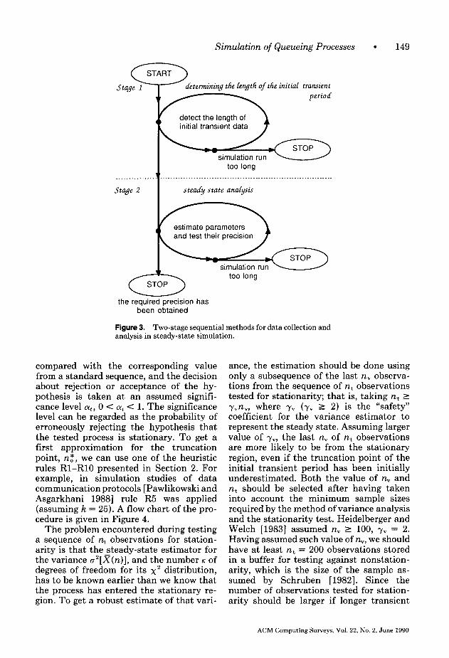
Simulation of Queueing Processes l 149
&tenining the Gqgth qf the initiaf transient
detect the length of initial transient data
simulation run too long
1’ _____.._........ . . . . . . . . . . . . . . . . . . . . . . . . . . . . . . . . . . . . . . . . . . . . . . . . . . . . . . . . . . . . . . . . . . .
Stage 2 steady state analysis
estimate parameters and test their precision
the required precision has been obtained
Figure 3. Two-stage sequential methods for data collection and analysis in steady-state simulation.
compared with the corresponding value from a standard sequence, and the decision about rejection or acceptance of the hy- pothesis is taken at an assumed signifi- cance level Q, 0 < CY~ < 1. The significance level can be regarded as the probability of erroneously rejecting the hypothesis that the tested process is stationary. To get a first approximation for the truncation point, n,*, we can use one of the heuristic rules Rl-RlO presented in Section 2. For example, in simulation studies of data communication protocols [Pawlikowski and Asgarkhani 19881 rule R5 was applied (assuming k = 25). A flow chart of the pro- cedure is given in Figure 4.
The problem encountered during testing a sequence of n, observations for station- arity is that the steady-state estimator for the variance a2[X(n)], and the number K of degrees of freedom for its x2 distribution, has to be known earlier than we know that the process has entered the stationary re- gion. To get a robust estimate of that vari-
ance, the estimation should be done using only a subsequence of the last n, observa- tions from the sequence of n, observations tested for stationarity; that is, taking n, 2 yvnv, where yV (7” > 2) is the “safety” coefficient for the variance estimator to represent the steady state. Assuming larger value of yV, the last n, of n, observations are more likely to be from the stationary region, even if the truncation point of the initial transient period has been initially underestimated. Both the value of n, and n, should be selected after having taken into account the minimum sample sizes required by the method of variance analysis and the stationarity test. Heidelberger and Welch [1983] assumed n, 2 100, yV = 2. Having assumed such value of n,,, we should have at least n, = 200 observations stored in a buffer for testing against nonstation- arity, which is the size of the sample as- sumed by Schruben [1982]. Since the number of observations tested for station- arity should be larger if longer transient
ACM Computing Surveys, Vol. 22, No. 2, June 1990

150 l Krzysztof Pawlikowski
apply a heuristic rule for discarding observations collected during the initial transient period
collect new observations
4
Welch [1981a], based on the spectral analy- sis of observations, was used in simulation studies of data communication protocols [Asgarkhani and Pawlikowski 1989; Paw- likowski and Asgarkhani 19881 and is sum- marized in Appendix B.
Having estimated the variance, which by assumption represents steady state of the process, we can start testing the first n, observations for stationarity. If the test accepts the hypothesis that the end of the initial transient has been detected correctly and the process has already entered its stationary region, this stage of analysis of the simulation output results is finished and the program may start to analyze con- fidence intervals; see Section 3.2. Otherwise transient effects have still been detected. Consequently, additional rno* observations
test stationarity of the next from the beginning of the test sequence are
nt observations discarded, rno* new observations are col- lected, the last n, observations are again used to estimate (~‘[X(n,)l, and the first n, observations in the stored sequence are
discard a number of observations
tested for stationarity. This procedure is
l from beginning of continued until the stationarity of the tested sequence sequence of observations is confirmed or
n O,mBx (the upper limit of the number of tested observations) is reached. As the
the length of the initial longest acceptable length of the initial tran- transient has been found,
start steady state simulation sient period, one can assume no,max = 0.5nmax, where nmax is the maximum length of the simulation run. If the transient phase
Figure4. Sequential analysis of the length of the extends beyond no,,,ax observations, either initial transient period. the allowed maximum length of the simu-
lation run is too short or the system is unstable.
periods are suspected, one can assume that Summing, up, the procedure requires the
nt = max(wb, v-0, (76) following parameters:
where rnt is the smallest length of one step nmax The maximum allowed length of the
in sequential testing for stationarity for a simulation run measured in the number
given n,*, y > 0. of recorded observations (to be decided
Thus, after having discarded n,* obser- in advance. In simulation studies re-
vations, the next n, observations are col- ported in Asgarkhani and Pawlikowski
lected and the last nv observations are used [ 19891 and Pawlikowski and Asgarkhani
to find G2[x(n)] and K. The variance and [ 19881 nmax was not less than 100,000);
the degrees of freedom of its x2 distribution kmax The maximum allowed length of the can be estimated using a few differ- initial transient period (the default value ent methods, presented, for example, in is no,msx = 0.5%& Fishman [1973a, p. 2891, Heidelberger and n, The length of the sequence used for Welch [1981a], and Schruben [1982]. The estimating the steady-state variance method described by Heidelberger and a2[X(n)] (the default value is n, = 100).
ACM Computing Surveys, Vol. 22, No. 2, June 1990

Simulation of Queueing Processes l 151
n, The length of the sequence tested for stationarity; see Equation (76).
LY~ The significance level of the station- arity test (0 < olt < 1; the default value is q = 0.05).
yV The “safety” coefficient for the esti- mator of variance a’[X(n)] to represent the steady state (yy z 2; the default value is yV = 2).
y The “exchange” coefficient, determin- ing the number of new observations included in each sequential test for stationarity (y > 0; the default value is y = 0.5).
The procedure can be described as follows:
procedure DetectInitial Transient; {determine the length of the initial period apply- ing the Schruben’s test preceded by an heuristic rule of truncation)
Step 1 Start the simulation run from the empty-and-
idle state; apply one of the heuristic deletion rules Rl-
RlO (see Section 2) to determine n,*; (no* is the first approximation of the number of observations to be deleted)
if (the initial transient period embraces more than no.max observations) then goto Step 6
else n, := n,*; discard first n, observations endif; if yvn,, 2 ynz then nt := yvn, else n, := -ynX
endif; A, := yn,*; (n, observations will be tested for
stationarity, A,, old observations will be replaced by new ones)
at, := a,; (the initial value of significance level of the test for stationarity; see Step 4 )
Step 2 If n, + n, 5 qmax then
append A,, observations to the tested se- quence; (some of these observations may have been already collected when the heuristic deletion rule was applied)
got0 Step 3 else (if n, + nt > nO,m.xl
goto Step 6 endif;
Step 3 Determine the variance ?[X(n,)] and K, the
degrees of freedom of the variance distri- bution, using the last n, collected observa- tions starting from the observation (n, + n, - n, + 1);
(for example, apply the procedure Spectral- Variance Analysis described in Appendix B, as- suming I, = x,~+ n,--ny +s, for s = 1, 2, . . . , n,)
Step 4 (the test for stationarity [Schruben et al. 1983, p. 117311
Take all n, observations, starting from the ob- servation (n, + l), and calculate the test sta- tistic
T= JZ
z k nt%~5G[X(n,)] A=1
",-tL
where x(i) = C ?; j=no+l 1
if (a negative bias of the mean X(n,) is sus- pected)
then goto Step 5 elsif (a positive bias is suspected) then T := -T (the reason for considering bias of an assumed sign is that one-sided tests are usually more powerful than their two-sided correspondents) else (if a sign of the initial bias is difficult to
predict, then prepare data for a two-sided test)
T:= 1 TI; atI := a,/2 endif;
Step 5 if T 5 t,,l-,,, then
k-a,, is the upper (1 - a,J critical point from the t-distribution with K degrees of freedom)
write (‘the initial transient period is not longer than n, observations’);
start sequential analysis of confidence inter- vals
(call one of procedures presented in Section 3.2)
else {if T > tx.l-n,,l discard first rn$ observations from the tested
sequence; no := n, + yn,*; A,, := yn,*; goto Step 2
endif
Step 6 (if the initial transient period embraces more than no,max observations)
stop the simulation run; write (‘the initial transient period embraces
more than no,mex observations, or the simulated process is unstable ‘)
end DetectInitialTransient.
ACM Computing Surveys, Vol. 22, No. 2, June 1990

152 l Krzysztof Pawlikowski
The effectiveness of this procedure strongly depends on the effectiveness of the variance estimator G2[X(n)]. transient period have been
3.2 Sequential Testing for a Required Precision of Results
Both sequential procedures for stopping a simulation experiment that are presented here require the analyzed sequence of observations to be representative of steady state, so no observations representing the initial transient period have to have been discarded beforehand.
The first procedure is a modified version of the spectral method of analysis proposed by Heidelberger and Welch [1981a, 1981b, 19831. Its simplified flow chart is given in Figure 5. As mentioned in Section 1, the method allows the reduction of the number of individual data items stored in memory during a simulation experiment by batching individual observations into batches of size 2m, m = 1,2, . . . , and replacing them with
collect more observations 1
1 determine steady state estimators and test their
precision
Yes
parameters have been The required precision
the batch means. These means are stored in the buffer AnalysedSequence of size 2M. Whenever 2M batch means over batches of m observations are recorded, they are con- solidated into M means over batches of size
can not be reached
Figure 5. Flow chart for the spectral method.
2m. Subsequent observations are lumped into M successive batches of size 2m. If utive checkpoints, one can assume w1 =
more than M such new batches are needed, max(2M, 2nJ and a constant value for the
the rebatching procedure is repeated. Thus, step between checkpoints above a threshold
the buffer AnalysedSequence can be imple- point. Following a different reasoning, se-
mented simply as a one-dimensional array lection of the value of u1 satisfying the
of size 2M. The accuracy of estimators is inequality
measured by the relative precision E of con- fidence intervals, defined in Equation (12), and the simulation is stopped if E % emax, where t,,, is the acceptable maximum value of the relative precision of the final results. The current values of 6 are evaluated at consecutive checkpoints wk (k = 1, 2, . . . ; Ok 5 nmax); that is, each time (wk+l - wk) new observations have been collected. To limit the number of possible checkpoints, one can assume that they are geometrically distributed; that is, for a given wi,
where k = 1,2, . . . ; L3cJ denotes the greatest integer not greater than x and y. > 1. To avoid too large a distance between consec-
ok+1 = minil-fduk - n& + no, nmaxj, (77)
LO.l(n,,, - n,)l
+ n, 5 01 5 LO.2(12,,, - n,)J + n, (78)
was suggested in Heidelberger and Welch [1983]. The estimator of variance a2[X(n)]
n,,
and the number K of its degrees of freedom needed in analysis of confidence intervals
The number of discarded initial obser-
are calculated here using the procedure SpectralVarianceAnaiysis. It requires at
vations (determined by the procedure
least n, > 100 batch means to be available (see Appendix B). This approach is de-
DetectInitialTransient).
scribed below by a pseudocode procedure that uses the following parameters:
ACM Computing Surveys, Vol. 22, No. 2, June 1990

Simulation of Queueing Processes l 153
nmax The maximum allowed length of the simulation run, measured in the num- ber of recorded observations (nmax 2 max(3n,, n, + 2M); to be decided in advance).
n, The length of the sequence used for estimating the variance 02[X(n)] (G 2 100; the default value is n, = 100).
ya The checkpoint incremental coeffi- cient for sequential testing for accuracy (ya > 1; the default value is ya = 1.5).
(1 - a) The assumed confidence level of the final results (0 < 01 < 1; the default value is 01 = 0.05).
t,,, The maximum acceptable value of the relative precision of confidence inter- vals (0 < emax < 1; the default value is: emax = 0.05).
procedure SpectralAnalysis; (sequential analysis of simulation output data based on spectral analysis of the series of col- lected obseruations)
const M = 100; (the default value of the minimum number of data points for the analysis of confidence in- tervals; M z n, 2 100; see Section 3.1)
procedure Batching; (preparation of secondary output data; transfor- mation of individual observations into the se- quence of no more than 2M batch means of sequentially increasing batch size)
begin (calculate the batch mean xj(m), and store it as the jth data item in the buffer AnalysedSequence)
Xj(l72) := sum/m; if j = 2M then {consolidate 2M means of
batches of site m into M means of batches of size 24
for s := 1 to M do XJ2m) := 0.5(Xz~-,.-,(m) + X&m))
enddo
m:=2m;j:=M endif j:=j+l;sum:=O
{start to calculate the next batch mean end Batching;
procedure Estimation; (sequentially calculate estimates and test their precision until the required precision is reached)
begin find the estimator G2[X(n,)] for the sequence
xj-nv+,(m), . . . , Xj(m), the last n, batch
means stored in the buffer Analysed- Sequence, and determine K, the degrees of freedom of the distribution of f3Xh)l; (apply the procedure SpectralVariance- Analysis; see Appendix B ) calculate the relative half width of the confidence interval at the confidence level (1 - LY) for the current check- point wk:
c = tK,I-,~2~[X(nv)llX( jm),
where x( jm) = CJ’=, xs(m)/j
is the current value of the estimated mean after jm observations, and t.,l-.,2 is the upper (1 - a/2) critical point of the t- distribution with K degrees of freedom;
(test conditions of stopping the simulation run) if (t 5 fmax) then
(print the final results and stop the simula- tion)
StopSimulation := true else (the required precision has not been
reached yet; determine the next, (k + l)st, checkpoint)
k := k + 1; wk := min(ty.(w&l - &,)A + n,,, nmax)
endif end Estimation;
begin (main procedure) m := 1; {the initial batch size) k := 1;
(the initial checkpoint is after 6& = w1 obser- vations)
w, := n,; i := 1; (having discarded n, observations, collect next observations starting from the obser- vation (w, + i))
w1 := max(2M, 2n,); (the default location of the first checkpoint]
sum := 0; j := 1; (start calculating the 1st batch mean)
StopSimulation := false; {a condition of stopping the simulation has not been met yet)
while (not StopSimulation) do (collect and process new (wk - w&-l) obser- uations)
get the observation x,~+;; sum := sum + x,~+,; if (i mod m = 0) then Batching endif; if (i = WJ then Estimation endif; if (not StopSimulation) then
i := i + 1; if (i > nmsx - n,) then
write (‘the required accuracy cannot be reached; either restart the simulation
ACM Computing Surveys, Vol. 22, No. 2, June 1990

154 l Krzysztof Pawlikowski
using a new seed (seeds) of random number generator, or increase n,ax, or zncrease a, or mcrease cmax 7;
{for obtaining a new sequence of pseu- dorandom numbers, independent from the previous one, assume the last num- ber from the previous sequence as the first number of the new sequence] StopSimulation := true
endif endif
enddo; write (‘the required precison of results has
been obtained having collected’, n, + jm, ‘observations; the final relative precision:‘, loot%, ‘the final (1 - a)lOO% confidence interval:‘, X( jm)[l f t])
end SpectralAnalysis.
The next sequential procedure for stop- ping simulation experiments when the re- quired precision of results is reached is based on the method of nonoverlapping batch means. Its simplified flow chart is given in Figure 6 (only the main loops of computations are depicted). As in the case of the procedure SpectralAnalysis, the initial nonstationary sequence of n, ob- servations should have been discarded earlier, applying, for example, the proce- dure DetectInitialTransient. For weaken- ing serial correlations of analyzed output data, individual observations are replaced here by the less correlated means of their batches. Thus, the problem of direct analy- sis of confidence intervals from correlated observations is replaced by the problem of determining the batch size m*, such that batch means are (almost) uncorrelated at a given level of significance. Generally, in a sequence of correlated data the autocorre- lation coefficients of lag k, k = 1, 2, . . . , [see Equations (21) and (22)] are not nec- essarily decreasing as the lag increases, al- though all autocorrelation coefficients are zero if the sequence contains uncorrelated observations. For this reason, we follow the test proposed by Adam [1983]: A given batch size can be accepted as the batch size for approximately uncorrelated batch means if all L autocorrelation coefficients of lag k (k = 1, 2, . . . , L) are statistically negligible at a given significance level Pk, 0 c /3k < 1. The analytical problems en- countered during estimation of the auto-
correlation coefficients suggest that the number of considered lags should be limited to L = 0.1 kbo, where kbo is the number of batch means tested for autocorrelation; see comments in Section 1. The autocorrela- tion coefficients can be better estimated by the so-called jackknife estimators [Miller 19741, which are usually less biased than the ordinary estimators defined by Equa- tions (21) and (22). A jackknife estimator of autocorrelation coefficient of lag k for a sequence of batch means of size m is cal- culated from the following formula:
F(k, m)
?‘(k, m) + i”(k, m) (79) = 2i(k, m) -
2 ,
where the estimators on the right-hand- side are calculated like ordinary estimators of autocorrelation coefficients [see Equa- tions (21) and (22)], except that i(k, m) is the estimator over all kbo batch means, whereas i’(k, m) and i”(k, m) are esti- mators over the first and the second half of the analyzed sequence of kbo batch means, respectively.
Let us note the following:
(i) To get acceptable estimators of the au- tocorrelation coefficients, at least 50 batch means should be available [Box and Jenkins 1970, p. 331; thus, in the case of jackknife estimators one should assume kbO 2 100. (ii) To ensure approximate normality of batch means, the size of considered batches should not be less than 50 [Adams 19831. (iii) To get an acceptable overall signifi- cance level p when testing the value of L autocorrelation coefficients of lag k (k = 1, 2 > .-., L), each at the significance level Pk, we have to assume
PC c Pk, k=l
hence in practice L should not be too large. This restriction is irrelevant if the autocor- relation coefficients decrease monotoni- cally with the value of the lag, since then only F(1, m) has to be considered.
ACM Computing Surveys, Vol. 22, No. 2, June 1990

Simulation of Queueing Processes l 155
test autocorrelation within the FHpi2iips
estimated with
Figure 6. Flow chart for the method of batch means.
To avoid wastefully collecting an exces- (s = 1, 2, . . .), formed from the batch means sive number of observations, especially kept in the Referencesequence. Thus, since when testing batch sizes, the procedure the number of data items collected in the BatchMeansAnalysis uses two buffers for Referencesequence grows in time during a storing batch means: A buffer called simulation run, a linked list of batch means Referencesequence is used to store the seems to be a proper data structure for this batch means X(m,), x2(mO), . . . of a batch buffer. The number of data items in the srze m,, and a buffer AnalysedSequence is AnalysedSequence is limited to kbo, so used for storing an assumed number kbo of it can be implemented as an ordinary batch means over batches of size m, = sm, one-dimensional array. By selecting m,
ACM Computing Surveys, Vol. 22, No. 2, June 1990
156 . Krzysztof Pawlikowski
properly, we can secure a sequential in- crease of tested batch sizes slower than in the batching schemes proposed in Adam [ 19831, Fishman [1973a], Law and Carson [1979] to reduce the resultant simulation run length. For neutralizing the observed randomness of the estimators of correlation coefficients, m* = m, is selected as the final batch size of weakly correlated means iff the hypothesis of all zero autocorrelation coefficients is accepted in two succesive tests, both for the batch size rnSml and m,.
Having selected the batch size m*, one can sequentially analyze the accuracy of results by calculating confidence intervals from Equations (18) and (19), which are valid for independent and identically dis- tributed batch means. The sequence of batch means for batch size m* kept in the buffer ReferenceSequence can be sequen- tially appended by new batch means if more observations are needed to improve the ac- curacy of results. As mentioned in Section 1, Schmeiser [1982] showed that using 10 to 30 batch means over longer batches can give more accurate results (and a better coverage of the estimators) than using more batch means over smaller batches. Follow- ing these recommendations, when the ac- curacy test of the estimator from kbe batch means stored in the ReferenceSequence fails, these kbe batch means are used to form kbo = 30 batch means in the Analysed- Sequence buffer for the additional accuracy test. Such a test is done before a new batch mean is appended to the Reference- Sequence.
The whole method can be summarized by the following pseudocode procedure, which requires these parameters:
rz, The number of discarded initial obser- vations (determined by the procedure DetectInitialTransient).
nmax The maximum allowed length of the simulation run, measured as the number of recorded observations (r~,~, > n, + m,kbo; to be determined in advance).
1-CY The assumed confidence level of the final results (0 < cy < 1; the default value is o( = 0.05).
emax The maximum acceptable value of the relative precision of confidence inter- vals (0 < t,,, < 1; the default value is Emax = 0.05).
The initial values of other parameters are given in the procedure.
procedure BatchMeansAnalysis; (sequential analysis of simulation output data based on analysis of uncorrelated means of non- overlapping batches of observations)
const m, = 50; (the default value of the batch size for means stored in the ReferenceSequence)
kb, = 100; (the default value of the number of batch means stored in the AnalysedSequence]
procedure DetermineBatchSize; (determine the batch size for approximately un- correlated batch means)
begin s:=l;j:=l;sum:=O;
{these are the initial values of parameters for determining x,(mJ, the jth batch mean of size m,, at the sth sequential step)
while ((not StopSimulation) and (not Un- correlated)) do
((i - 1) observations have been already re- corded)
for v := i to i + k&m, - 1 do {collect new kbomo observations for the next kbo batch means of size m, to be stored in the Referencesequence)
get the observation x,~+,; (the initial n, observations have been discarded)
sum := sum + x, +“; if (v mod m, = 6) then
(calculate the batch mean jrj(m,J; the jth data item in the Reference- Sequence]
Xj(m,) = sum/m,; sum := 0; j := j + 1 endif {the next batch mean has been
determined) enddo (the next kbo batch means have been
determined) for v := 1 to kbo do
(consolidate skb, batch means X,(m,), -%hL . . . , from the ReferenceSequence into kbo batch means P,(sm,), y2(sm,,), . . . . in the AnalysedSequence, which will be tested for autocorrelation)
TV(sm,) := CL XCv-l~s+r(mo)ls
ACM Computing Surveys, Vol. 22, No. 2, June 1990

Simulation of Queueing Processes l 157
enddo TestCorrelation; i := i + kbm,;
(r~,+~-, observations have been collected) if (not Uncorrelated) then
(re-initialize the counter variable for the next autocorrelation test 1
s := s + 1 endif if (not Uncorrelated) and (n, + i + k,m,
- 1 > nmax) then (stop selecting the batch size if the next test requires more than nmax observations]
write (‘the batch size of uncorrelated batch means cannot be determined tncrease nmax or p’); (p is the significance level of tests against autocorrelation used in the procedure TestCorrelation; see Eq. (80) I
StopSimulation := true endif
enddo (of search for the batch size of uncor- related batch means]
end DetermineBatchSize;
procedure TestCorrelation; (test significance of autocorrelations between batch means for a given batch size)
const L = 10; (the default number of autocorrelation coeffi- cients; if autocorrelation coefficients mono- tonically decrease with the value of lag take L = 1, else L := 0.1 kb,]
f3 = 0.1; {the default value of the overall signif- icance level of L tests against autocor- relation]
begin Correlation := 0; (the initial value for testing
L correlation coefficients) for k := 1 to L do
(test whether all L autocorrelation coeffi- cients are statistically negligible each at the ,& significance level)
calculate the jackknife estimator ;(k, sm,) of the autocorrelation coefficient of lag k for the sequence yI,(sm,), ~Jsm,), . . . , ~k,(sm,) stored in the Analyzed- Sequence; (apply Eq. (79) for m = sm,) Pk := P/L; P[i(k, sm,)] :=
if (k = 1) then (l/k,) else ([l + 2 C&i ?(u, sm,)]/kbO)
endif {the variance of the autocorrelation coef- ficient of lag k [Bartlett 194611
if ( I b, sm,) I < .G-P,/Z G[h smJ1) bw2 is the upper (1 - P&/2) critical point of the standard normal distribution)
then i(k, sm,) := 0 endif (the lag k autocorrelation is statisti-
cally negligible at the confidence level 1 - &)
Correlation := Correlation + ) i(k, sm,) ]; enddo if ((Correlation = 0) and AcceptableSize)
then {accept the current batch size since the pre- vious batch size has already given negligible correlations]
m* := sm,; Uncorrelated := true {the batch size m* of uncorrelated batch means has been selected 1
elsif (Correlation = 0) then (start collecting next observations for testing larger batch size)
AcceptableSize := true (autocorrelations for the current batch size are negligible but they were not negligible for the previous batch size, thus the next batch size should be considered)
endif end TestCorrelation;
procedure Estimation; (sequentially calculate estimates and test their precision until the required precision is reached) begin
calculate the mean %(k&, m), its variance
(TP[??(kbe, m)], and the relative half width e of the confidence intervals at the confidence level (1 - a):
using the whole sequence of kbe data items stored in the Referencesequence: {apply Eqs. (17)-(19), for kb := kbe, m := m* and xi(m) := x;(rn*))
if ((t > emax) and (kb mod 30 = 0)) then (the additional test of accuracy of estimators after consolidation of k& batch means from the ReferenceSequence into kbo = 30 means of longer batches stored in the Analysed- Sequence; see the recommendations in Schmeiser [1982] )
m := kb,/30;
ACM Computing Surveys, Vol. 22, No. 2, June 1990

158 l Krzysztof Pawlikowski
forj:=lto30do
calculate the mean x( kbo, mm*), its vari- =
ante G2[X(kb0, mm*)], and the relative half width 6 of the confidence interval at the confidence level (1 - a):
t :=
tkb--l.l-a,24~(kbo, mm*)ll~(kh, mm*),
from the sequence of 30 data items stored in the AnalyzedSequence; (apply Eqs. (17)-(19), for kbo := 30, m := mm*, X,(m) := Ti(mm*))
enddo endif if (6 5 t,,& (the required precision has been
reached 1 then write (‘the required precision of re- sults has been obtained after’, n, + kbem*, ‘observations recorded ‘); StopSimulation := true
elsif (n, +,(kbe + l)m* I n,,,) then (kbe batch means of size m* have been used to estimate the mean FU, but the required precision has not been reached yet; collect the next batch of m* observations and store their mean in the ReferenceSequence]
sum := 0; for j := 1 to m* do
get the observation xkbm*+j; sum := sum + Xk,,*+j
enddo k, := kbe + 1; &Jm*) := sum/m*
else (the required precision has not been reachecl, too short the simulation run assumed )
write (‘the required accuracy cannot be reached; either restart the simulation using a new seed (seeds) of random number generator, or increase nmsX, or Lncrease a, or mcrease cmex ‘1;
(for obtaining a new sequence of pseu- dorandom numbers, independent from the previous one, assume the last num- ber from the previous sequence as the first number of the new sequence)
StopSimulation := true endif
end Estimation;
ACM Computing Surveys, Vol. 22, No. 2, June 1990
begin (main procedure] StopSimulation := false;
(a condition of stopping the simulation has not been met yet}
AcceptableSize := false; {a batch size for uncorrelated batch means has not been found yet)
Uncorrelated := false; (the batch size for uncorrelated batch means has not been determined yet]
t := 1 - t,.,; (the initial precision t > cmor ] i := 1; (having discarded n, observations, col-
lect the next observations starting from the observation (n, + 1)st)
DetermineBatchSize; {if the batch size m* has been selected then the ReferenceSequence contains skbo batch means of size m*/s and the AnalysedSequence contains kbo batch means of size m*)
kbe := k,,; (the size of the ReferenceSequence at the beginning of estimation)
for j := 1 to kbe do (prepare data for estimation; consolidate skbo batch means of size m, = m*/s in the ReferenceSequence into kbe = kbo batch means of site m*)
xj(m*) := CF=I ~tj-l)s+r(mo)/S
enddo while (Uncorrelated and
(not StopSimulation)) do
(sequentially test the precision of the esti- mators until the required precision or the maximum length of simulation run is reached)
Estimation; enddo write (‘the final relative precision:‘, loot%,
‘the final lOO(1 - a)% confidence inter-
val: ‘, .??(kbe, m*)[l + t]); end BatchMeansAnalysis.
In practice, the last procedure often uses a sequential search for the batch size of uncorrelated batch means rather than the sequential stopping rule for the simulation run (sequential testing the precision of es- timates). This happens because usually many more batch means have to be tested

Simulation of Queueing Processes l 159
during the first stage (testing against au- tocorrelation) than during the second stage (testing the precision of the results). The number of observations recorded, kbom*, when the mean and the width of confidence intervals are to be calculated for the first time is usually much larger than is required for obtaining the required level of accuracy [Schmeiser 19821. From this point of view, the spectral method of analysis is more thrifty. On the other hand, the method of batch means uses a very simple estimator of the variance when the width of confi- dence intervals is analyzed. Exhaustive comparative studies of both procedures have not been performed yet, but the re- ported results indicate that the spectral method is usually more efficient, both in the sense of the coverage recorded in ref- erence experiments and in the sense of the final simulation run lengths for obtaining the required accuracy of the results, at least in investigated classes of processes [Pawlikowski and Asgarkhani 19881.
4. SUMMARY AND GENERAL COMMENTS
We have discussed in detail methods for dealing with the main phenomena encoun- tered in steady-state simulation of queuing processes: the inherent initial nonstation- arity and the permanent autocorrelation of collected observations. The emphasis is on methods for the sequential analysis of sim- ulation output data, bearing in mind their possible implementation in user-friendly simulation packages, which would produce results automatically. In such a context, methods of analysis based on single simu- lation runs seem to be more attractive than the methods of independent replications.
This survey has been limited to analysis of a single measure of performance, namely, the point and interval estimates of the sam- ple mean. Nevertheless, this methodology can easily be modified to estimate other performance measures, as long as their es- timators are based on cumulative statistics. For example, sequential analysis of simu- lation output data can easily be applied to estimate the variance, or the probability that the analyzed variate lies in some fixed
interval [Welch 1983, Sec. 6.31. It cannot be applied directly to estimate quantiles, since their estimators require that se- quences of collected observations be pre- sorted and as such are not amenable to cumulative statistics calculated while the simulation is in progress. Estimation of quantiles by using the method of spectral analysis is discussed in Heidelberger and Lewis [1984]; the same application of the regenerative method is considered in Igle- hart [1976] and Seila [1982a]. Computa- tional problems associated with quantile estimation are discussed in Jain and Chlamtac [ 19851 and Raatikainen [ 1987, 19881.
The methodology of simultaneous analy- sis of more than one measure of perfor- mance during one simulation experiment is much less advanced than the methodology of univariate estimation discussed in this paper. The main theoretical problems of multivariate estimation and the methods that can be used for determining the con- fidence regions in such multiresponse sim- ulation experiments are discussed in Charnes and Kelton [1988], Chen and Seila [ 19871, Friedman [ 19841, Law and Kelton [1982a, p. 3081, and Seila [1982b, 19831. The initialization bias in multiresponse simulation can be controlled by applying a statistical test proposed by Schruben [ 19811. Various variance reduction tech- niques that are applicable in this kind of simulation experiments are discussed in Bauer et al. [ 19871, Rubinstein and Marcus [ 19851, Venkatraman and Wilson [ 19861, and Yang and Nelson [ 19881.
Specific statistical problems accompa- nying comparative simulation studies of al- ternative systems are surveyed in Law and Kelton [1982a, Chap. 91; see also Balmer [ 19871, Clark [1986], Friedman and Fried- man [ 19861, and Goldsman [ 1983, 19861. (Note that in these applications the bias of estimators is not important, as long as the estimators are equally biased.) Stochastic simulation is also used for sensitivity analy- sis of performance measures and optimi- zation of various systems and processes under uncertainty. Special methods for es- timating the gradient of a performance measure with respect to a selected input
ACM Computing Surveys, Vol. 22, No. 2, June 1990

160 l Krzysztof Pawlikowski
parameter (e.g., the changes of the mean delay of messages in a communication net- work with respect to the mean message length) during a single simulation run are discussed in [Ho 1987; Ho and Cao 1983; Ho et al. 1983; Reiman and Weiss 1986; Rubinstein 1989; Suri and Zazanis 19881.
This paper is restricted to the statistical analysis of simulation output data, but practitioners are aware that that is not the only problem that must be overcome in obtaining useful results. Before observa- tions are collected, the processes for which performance is to be investigated have to be properly modeled, and each model should be validated and verified to make the simulation experiments credible. Var- ious aspects of the validation and verifica- tion of simulation models are discussed in [Banks and Carson 1984; Bulgren 1982; Law and Kelton 1982a; Sargent 1986; Shannon 1981; Velayas and Levary 19871.
Having presented methods of data collec- tion and analysis that are used in stochastic steady-state simulation, one can conclude that no definite conclusions can be made about their applicability. The need for more exhaustive comparative studies expressed by Schriber and Andrews [ 19811 still seems to be a live issue.
The length of simulation runs remains a critical issue, especially in the case of sim- ulation studies of complex systems, which often can be performed only if a technique for speeding up the process of data collec- tion is applied. In this context an important role could be played by the variance reduc- tion techniques, which, by reducing the variance, narrow confidence intervals and consequently reduce the number of steps needed by sequential procedures for reach- ing the required accuracy of results. But, as was mentioned in the Introduction, practi- cal implementations of variance reduction techniques have been reported infre- quently. Among the recently published ones are those in Izydorczyk et al. [1984] and Walrand [ 19881. Another area in which the duration of simulation can be very crit- ical is the analysis of performance measures that depend on events occurring infre- quently. Some techniques proposed for speeding up rare events simulation are
discussed in Cottrell [1983], Parekh and Walrand [1989], and Shahabuddin et al. [1988].
Performance evaluation studies based on simulation experiments can be accelerated by the decomposition of analyzed systems into subsystems, which are modeled sepa- rately, applying both simulation and ana- lytical models, mutually interacting if necessary. The efficiency of such an ap- proach was studied extensively in Blum et al. [ 19851 in the context of queuing network models of computer systems. A survey of hybrid techniques can be found in Shan- thikumar and Sargent [ 19831; see also Frost et al. [1988] and Kurose and Mouftah [1988]. The time needed for simulation studies can also be significantly reduced in multiprocessor systems. In such an envi- ronment individual processors can be used for running independent replications of one simulation experiment, or, in a more sophisticated solution, logical processes occurring during one simulation run can be executed in parallel by different proces- sors. The main problem encountered in the latter case is the synchronization among processes run on different processors. There exists a danger that the contribution of large synchronization overheads will actually slow the simulation experiment. Various techniques of distributed and par- allel simulation are discussed in Chandy and Misra [ 19811, Fujimoto [ 19881, Misra [ 19861, Nicol [1988a, 1988b], Reynolds [ 19881, Unger [ 19881, and Wagner and Lazowsa [1989]. See also Baik and Zeigler [ 19851, DeCegama [ 19871, Krishnamurthy et al. [ 19851, Kumar [ 19861, and Kurose and Mouftah [ 19881. Specific problems re- lating to the statistical analysis of output data that accompany distributed simula- tion are discussed in Heidelberger [ 19861.
The diversity of methodological ap- proaches and the complexity of some sta- tistical techniques used in simulation output analysis has motivated attempts to develop expert systems that give advice on selecting the best simulation methodology for accomplishing the required statistical computations; see, for example, Haddock [ 19871, Hahn [ 19851, Hand [ 19851, Nielsen [ 19861, and O’Keefe [ 19861. One of the first
ACM Computing Surveys, Vol. 22, No. 2, June 1990

Simulation of Queueing Processes l 161
statistical expert systems specifically ori- ented toward steady-state simulation is dis- cussed in Mellichamp and Park [1989]. It is hoped that further developments in the area of expert systems and applied statis- tics will make it possible to design fully automated, knowledge-based simulation packages.
APPENDIX A. ELEMENTARY STATISTICAL CONCEPTS
Appendix A contains elementary statistical concepts needed to understand the prob- lems discussed in this paper. A deeper and more detailed discussion of the subject can be found in the numerous textbooks such as [Trivedi 19821 on applied probability theory and statistics.
Stochastic simulation involves experi- ments that mimic various events by means of numbers generated by (pseudo)-random numbers generators. Therefore, it is natu- ral that the analysis of the output data should be based on the methods of statis- tical inference. These methods are applied to estimate the characteristics and/or pa- rameters of simulated processes. Accepting the random nature of simulation output data, one should consider any sequence x1, x2, -.*, x, of observations collected during such experiments as the sequence of reali- zations of random variables X, , XZ, . . . , X,, sampled from a stochastic process X(t) at instants of time t = ti, i = 1, 2, . . . , n. If the process X(t) is stationary, which means that its stochastic characteristics are time invariant, then the random variables X1, x2, ***, X,, have the same (but unknown) probability distribution. In the context of this paper, the process is stationary if it enters its steady-state region, and steady- state simulation is concerned with model- ing and analysis of such processes only.
Any function f (X, , X2, . . . , X,) of ran- dom variables X,, X2, . . . , X, is called a statistic. A statistic 0(X,, X,, . . . , X,) used for estimating a parameter 0 of the distri- bution of the analyzed process X(t) is called an estimator of 0. The number of independent random variables used in the definition of a statistic is called its number of degrees of freedom or, simply, its degrees
of freedom. The value 0(x,, x2, . . . , x,), that is, the value of function 0(X,, X2, . . . , X,) for a given sequence of observations x1, x2, . . . , x, is known as an estimate of 8. It means that estimators, as functions of ran- dom variables, are random variables them- selves, and estimates are simply reali- zations of these random variables.
A good estimator should be unbiased; see [Trivedi 19821 for other desired properties of estimators. If the estimator e^* = 6*(X1, x2, * * . , X,) of the parameter 0 is unbiased, then its statistical average
E[$*(X,, X,, . . . , X,)] = 0. (Al)
For example, it can be shown that the estimator it(n) given in Equation (1) is an unbiased estimator of the averageHpx of a stationary process X(t), since E[X(n)] = px. Similarly, one can show that if random variables X1, X2, . . . , X,, are independent and identically distributed, then the un- biased estimator of the variance u”[X] of the stationary process X(t) is
n (Xi - X(n))2 G”[X] = c (-42)
i=l n-l ’
while the unbiased estimator of the vari- ance of the estimator w(n) is
G”[X] G2[X(n)] = - *
n ’ (-43)
see Equation (4). Theoretical justification for using X(n)
as the estimator of y, is provided by the law of large numbers, which states that if ob- servations xl, x2, . . . , x, are realizations of independent random variables, taken from a stationary process X(t), then
lim P[] X(n) - pz 1 I C] = 1, (A4) n-m
for any c > 0. To construct confidence intervals for
X(n), we have to assume a probability dis- tribution for X(n). If x(n) is the weighted sum of independent and normally distrib- uted random variables Xi, i = 1, 2, . . . , n, with unknown variance u”[X], then it can be proved that the statistic
T _ = x(n) - P., n 1 G(n)1 W)
ACM Computing Surveys, Vol. 22, No. 2, June 1.990
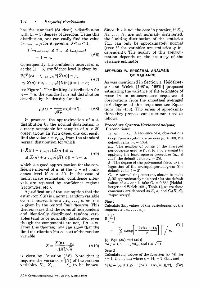
162 l Krzysztof Pawlikowski
has the standard (Student) t-distribution with (n - 1) degrees of freedom. Using this distribution, one can easily find the value t = tn--l,l--ai2 for it, given 01, 0 < o( C 1,
W-tn-p-n,2 -( Tn-, 5 tn--l,wd
= 1 - a!. (A@
Consequently, the confidence interval of p, at the (1 - a) confidence level is given by
RX(n) - LI,I-,,2m~)l 5 Px 5 X(n) + t,-l,J-,,~cqX(n)]) = 1 - a;
b47)
see Figure 1. The limiting t-distribution for n + ~0 is the standard normal distribution described by the density function
1 I&) = E exp(-z2). (A@
In practice, the approximation of a t- distribution by the normal distribution is already acceptable for samples of n > 30 observations. In such cases, one can easily find the value z = z~-,/~ from the standard normal distribution for which
5 X(n) + Z1--n,2G[x(n)]) = 1 - Ly. 649)
which is a good approximation for the con- fidence interval of pu, at the (1 - 01) confi- dence level if n > 30. In the case of multivariate estimation, confidence inter- vals are replaced by confidence regions (rectangles, etc.).
A justifi@ion of the assumption that the estimator X(n) is a normal random variable even if observations x1, x2, . . . , x, are not is given by the central limit theorem. This theorem says that the sums of independent and identically distributed random vari- ables tend to be normally distributed, even though the components are not, if n + to. From this theorem, one can show that the limit distribution (for n + 03) of the random variable
is given by Equation (A8). Note that it requires the variance u’[X] of the random variables Xi, X2, . . . , X,, to be known.
Since this is not the case in practice, if X1, x2, .*-, X,, are not normally distributed, the limiting distribution of the statistics T,-* can only be approximately normal (even if the variables are statistically in- dependent). The quality of this approxi- mation depends on the accuracy of the variance estimator.
APPENDIX 6. SPECTRAL ANALYSIS OF VARIANCE
As was mentioned in Section 1, Heidelber- ger and Welch [1981a, 1981b] proposed estimating the variance of the estimator of mean in an autocorrelated sequence of observations from the smoothed averaged periodogram of this sequence; see Equa- tions (45)-(50). The series of approxima- tions they propose can be summarized as follows.
Procedure SpectralVarianceAnalysis; (Preconditions:
Xl, x2,. . ., X”” A sequence of n, observations taken from a stationary process (n, 2 100, the default value: n, = 100). rzap The number of points of the averaged periodogram used to fit it to a polynomial by applying the least squares procedure (tzsp 5 rz,/4, the default value nap = 25). 6 The degree of the polynomial fitted to the logarithm of the averaged periodogram (the default value 6 = 2). C, A normalizing constant, chosen to make 6,(O) approximately unbiased (for the default values of nap and 6, take C, = 0.882 [Heidel- berger and Welch 1981, Table 11, where these constants are denoted as K, d, and C1(K, d), respectively) ]
Step 1 Calculate 2nnP values of the periodogram of the sequence x1, x2, . . . , x,“:
2xi(s - l)j ’
II/ W)
n” & {cf. Eqs. (45) and (46)) for j = 1, 2, . . . , 2nap, and i = &;
Step 2 Calculate nap values of the function (L(h)}, for j = 1, 2, . . . , n.,; where t; = (4j - l)/2nv, and
L(h) = log{[n(@j - l)/ny) + n(2j/ny)l/21; UW
ACM Computing Surveys, Vol. 22, No. 2, June 1990

Simulation of Queueing Processes l 163
Step 3 Apply the least squares extrapolation procedure {see, for example, Press et al. [1986, p. 5091) for determining the coefficient a, in the polynomial
(B3)
fitted to the function {L(f;) + 0.2701, j = 1, 2,
i thd :zLe a, is an unbiased estimate of log px (0) ]
Step 4 Calculate
fix(O) = C,e”o ; 034)
~:p[Xh)l = rjx(0)l%,; EW determine K;
(the degrees of freedom K for the x2 distribution of G&[X(n,,)], for given nap and 6, are given in Heidelberger and Welch 11981, Table 11 and de- noted there by C,(K, d ); for n, = 100, nap = 25 and 6 = 2: K = 7) end SpectralVarianceAnalysis.
If an analyzed sequence of output data consists of n, batch means XI(m), x,(m), . . . ) X,,” (m), each over m observations, in- stead of n, individual observations x1, x2, . . . , x,,” as above, the batch means should replace individual observations in Equation (Bl). Then the periodogram (II(j/n)) and the logarithm of the averaged periodogram (L(h)] are functions of the sequence XI(m), X2(m), . . . , XfV (m), and Equation (B4) gives us the estimate &cm,(O), the spectral density function of this sequence of batch means at f = 0. Now, with n, meaning the number of batch means, each over m obser- vations, we obtain
A(O) = wkd0); 036)
see Equation (49). Thus,-the estimator of the variance of the mean X(n,m), over n,m individual observations, is
G&[X(n,m)] = pxcm,o. (B7) n,
The degrees of freedom can be determined as in the previous case; see the comment in Step 4 of the procedure.
ACKNOWLEDGMENTS
I wish to thank my colleagues Tim Bell, Rod Harries, and Don McNickle for helpful comments during prep-
aration of this paper and Mehdi Asgarkhani and Tim Street for testing the sequential procedures presented. Special thanks are also due to two anonymous referees, whose comments greatly improved the final presen- tation.
REFERENCES
ABATE, J., AND WHITT, W. 1987a. Transient behav- ior of regulated brownian motion, I: Starting at the origin. Adv. Appl. Probab. 19, 560-598.
ABATE, J., AND WHITT, W. 198713. Transient behav- ior of regulated brownian motion, II: Non-zero initial conditions. Adv. Appl. Probab. 19,599-631.
ABATE, J., AND WHITT, W. 1987c. Transient behav- ior of the M/M/l queue: Starting at the origin. Queue. Syst. 2, 41-65.
ABATE, J., AND WHITT, W. 1988. Transient behavior of the M/M/l queue via Laplace transform. Adv. Appl. Probab. 20, 145-178.
ADAM, N. R. 1983. Achieving a confidence interval for parameters estimated by simulation. Manage. Sci., 29, 856-866.
AMEMIYA, T. 1973. Generalized least squares with an estimated autocovariance matrix. Econometria 41,723-732.
ANDERSON, K. 1985. Some steady-state problems in simulation. In Proceedings of the Annual Simu- lation Symposium (Tampa, Fla.). IEEE Computer Society, New York, 79-93.
ANDREWS, R. W., AND SCHRIBER, T. J. 1978. Interactive analysis of output from GPSS-based simulations. In Proceedings of the 1978 Winter Simulation Conference (Miami Beach, Fla.). ACM/IEEE, New York, 267-278.
ANONUEVO, R., AND NELSON, B. L. 1986. Auto- mated estimation and variance reduction for steady state simulation. In Proceedings of the 1986 Winter Simulation Conference (Washington, D.C.). ACM/IEEE, New York, 871-875.
Artificial intelligence and simulation: The diversity of applications. 1988. In Proceedings of the SCS Multiconference (San Diego, Calif.). Society for Computer Simulation.
ASGARKHANI, M., AND PAWLIKOWSKI, K. 1989. Simulation studies of mixed traffic on satellite channels using TDMA-reservation protocol. In Proceedings of the 8th Phoenix International Conference on Computers and Communications (Scottsdale, Ariz.). IEEE, Washington, D.C., 195-200.
BAIK, D., AND ZEIGLER, B. P. 1985. Performance evaluation of hierarchical distributed simulators. In Proceedings of the 1985 Winter Simulation Conference (San Francisco, Calif.). ACM/IEEE, New York, 421-427.
BALMER, D. W. 1987. Polishing the analysis of the statistical output of comparative simulation ex- periments. Simulation, 49, 123-126.
BANKS, J., AND CARSON, J. S. 1984. Discrete Event System Simulation. Prentice-Hall, Englewood Cliffs, N.J.
ACM Computing Surveys, Vol. 22, No. 2, June 1990

164 . Krzysztof Pawlikowski
BARTLETT, M. S. 1946. On the theoretical specifi- cation of the sampling properties of autocorre- lated time series. J. Roy. Stat. SOC. Ser. B, 8, 27-41.
BAUER, K. W., VENKATRAMAN, S., AND WILSON, J. R. 1987. Estimation procedures based on con- trol variates with known covariance matrix. In Proceedings of the 1987 Winter Simulation Con- ference (Atlanta, Ga.). ACM/IEEE, New York, 334-341.
BEALL, C. W. 1982. A regression technique or deter- mining steady state conditions in time series sim- ulations. In Proceedings of the 1982 Winter Simulation Conference (San Diego, Calif.). ACM/ IEEE, New York, 439-448.
BELL, P. C., AND O’KNEEFE, R. M. 1987. Visual interactive simulation: History, recent develop- ments, and major issues. Simulation, 49, 1099116.
BHARATH-KUMAR, K., AND KERMANI, P. 1984. Performance evaluation tool (PET): An analysis tool for computer communication networks. IEEE J. Select. Areas Commun. SAC-2, 220-225.
BILLINGSLEY, P. 1968. Conuergence of Probability Measures. Wiley, New York.
BLACKMAN, R. B., AND TUCKEY, J. W. 1958. The measurement of power spectra from the point of view of communications engineering (Part 1 and Part 2). Bell Syst. Tech. J. 37, 185-282, 485-569.
BLANC, J. P. C. 1985a. The transient behaviour of networks with infinite servers nodes. In Perfor- mance ‘84, E. Gelenbe, Ed. North Holland, Amsterdam, 159-174.
BLANC, J. P. C. 1985b. The relaxation time of two queueing systems in series. Commun. Statist. Sto- chastic Models 1, 1-16.
BLOMQVIST, N. 1967. The covariance function of the M/G/l queueing system. Skandinavisk Aktuarie- tidskrift, 6, 157-174.
BLOMQVIST, N. 1970. On the transient behavior of the GI/G/l waiting-times. Skandinavisk Aktua- rietidskrift, 53. 118-129.
BLUM, A., ET AL. 1985. Experiments with decompo- sition of extended queueing network models. In Modelling Techniques and Toots for Performance Analysis, D. Potier, Ed. North-Holland, The Netherlands, 623-638.
Box, G. E. P., AND JENKINS, G. M. 1970. Time Series Analysis, Forecasting and Control. Holden- Day, San Francisco.
BRATLEY, P., Fox, B. L., AND SCHRAGE, L. E. 1983. A Guide to Simulation. Springer-Verlag, New York.
BRILLINGER. D. R. 1973. Estimation of the mean of
BULGREN, W. G. 1982. Discrete System Simulation. Prentice-Hall, Englewood Cliffs, N.J.
CALVIN, J. M. 1988. Covariance of regenerative mean and variance estimators for the Markov chains. In Proceedings of the 1988 Winter Simu- lation Conference (San Diego, Calif.). ACM/ IEEE, New York, 473-475.
CARSON, J. S., AND LAW, A. M. 1980. Conservation Equations and Variance Reduction in Queueing Simulations. Oper. Res., 28, 535-546.
Catalog of simulation software. 1987. Simulation, 49, 165-181.
CHANDY, K. M., AND MISRA, J. 1981. Asynchronous distributed simulation via a sequence of parallel computations. Commun. ACM, 24,198-205.
CHARNES, J. M., AND KELTON, W. D. 1988. A com- parison of confidence region estimators for mul- &variate simulation output. In Proceedings of the 1988 Winter Simulation Conference (San Dieno. Calif.). ACM/IEEE, New Yo;k, 458-465. - ’
CHEN, D. R., AND SEILA, A. F. 1987. Multivariate inference in stationary simulation using batch means. In Proceedings of the 1987 Winter Simu- lation Conference (Atlanta, Ga.). ACM/IEEE, New York, 302-304.
CHENG, R. C. H. 1976. A note on the effect of initial conditions on a simulation run. Oper. Res. Quart., 24,467-470.
CHENG, R. C. H. 1986. Variance reduction methods. In Proceedings of the 1986 Winter Simulation Conference (Washington, D.C.). ACM/IEEE, New York, 60-68.
CLARK, G. M. 1986. A Bonferroni selection proce- dure when using common numbers with unknown variances. In Proceedings of the 1987 Winter Sim- ulation Conference (Washington, D.C.). ACM/ IEEE, New York, 313-315.
COHEN, J. W. 1982. The Single Sewer Queue. North- Holland, Amsterdam.
CONWAY, R. W. 1963. Some tactical problems in digital simulation. Manage. Sci., 10, 47-61.
CONWAY, R. W., JOHNSON, B. M., AND MAXWELL, W. C. 1959. Some problems of digital systems simulation. Manage. Sci. 6, 92-110.
COTTRELL, M., FORT, J. C., AND MALGOUYRES, G. 1983. Large deviations and rare events in the study of stochastic algorithms. IEEE Trans. Automatic Control, AC-28, 907-918.
Cox, D. R., AND SMITH, S. W. L. 1961. Queues. Wiley, New York.
CRANE, M., AND IGLEHART, D. L. 1974. Simulating stable stochastic systems: I. General multiserver aueues. J. ACM. 21, 103-113.
a stationary time series by sampling. J. Appl. Prob., 20, 419-431.
CRANE, M. A., AND IGLEHART, D. L. 1975a. Simulatine stable stochastic svstems: III. Resen-
BRILLINGER, D. R. 1981. Time Series: Data Analysis erative processes and discrete-event simulations. and Theory Holden-Day, San Francisco. Oper. Res., 23, 33-45.
BROCKWELL, P. J., AND DAVIS, R. A. 1987. Time CRANE, M. A., AND IGLEHART, D. L. 1975b. Series: Theory and Methods. Springer-Verlag, Simulating stable stochastic systems. IV: Approx- New York. imation techniques. Manage. Sci., 21, 1215-1224.
ACM Computing Surveys, Vol. 22, No. 2, June 1990

Simulation of Queueing Processes 165
CRANE, M. A., AND LEMOINE, A. J. 1977. An Intro- duction to the Regenerative Method for Simulation Analysis. Lecture Notes in Control and Informa- tion Science, No. 4, A. W. Balakrishnan and M. Thoma, Eds. Springer-Verlag, New York.
DALEY, D. J. 1968. The serial correlation coefficients of waiting times in a stationary simple server queue. J. Austral. Math. SOC., 8, 683-699.
DAMERDJI, H. 1987. On strong consistency of the variance estimator. In Proceedings of the 1987 Winter Simulation Conference (Atlanta, Ga.). ACM/IEEE, New York, 305-308.
DECEGAMA, A. 1987. Parallel processing simulation of large computer networks. In Proceedings of the 1987 Symposium on the Simulation of Computer Networks (Colorado). ACM/IEEE, New York, 51-62.
DONNELLY, J. N., AND SHANNON, R. E. 1981. Minimum mean-squared error estimates for simulation experiments. Commun. ACM, 24, 253-259.
DUERSCH, R. R., AND SCHRUBEN, L. W. 1986. An interactive run length control for simulations on PCs. In Proceedings of the 1986 Winter Simula- tion Conference (Washington, D.C.). ACM/IEEE, New York, 866-870.
DUKET, S. D., AND PRITSKER, A. A. B. 1978. Examination of simulation output using spectral methods. Math. Comput. Simul., 20, 53-60.
EMSHOFF, J. R., AND SISSON, R. L. 1970. Design and Use of Computer Simulation Models. Mac- millan, New York.
FISHMAN, G. S. 1967. Problems in the statistical analysis of simulation experiments: The compar- ison of means and the length of sample records. Commun. ACM, 10,94-99.
FISHMAN, G. S. 1971. Estimating sample size in computing simulation experiments. Manage. Sci., 18,21-38.
FISHMAN, G. S. 1972. Bias considerations in simu- lation experiments. Oper. Res., 20, 685-790.
FISHMAN, G. S. 1973a. Concepts and Methods in Discrete Event Digital Simulation. John Wiley, New York.
FISHMAN, G. S. 1973b. Statistical analysis for queueing simulation. Manage. Sci., 20, 363-369.
FISHMAN, G. S. 1974. Estimation in multiserver queueing simulations. Oper. Res., 22, 72-78.
FISHMAN, G. S. 1977. Achieving specific accuracy in simulation output analysis. Commun. ACM, 20,310-315.
FISHMAN, G. S. 1978a. Principles of Discrete Event Simulation. John Wiley, New York.
FISHMAN, G. S. 1978b. Grouping observations in digital simulation. Manage. Sci., 24, 510-521.
FISHMAN, G. S., AND KIVIAT, P. J. 1967. The analy- sis of simulation-generated time series. Manage. Sci., 13, 525-557.
FOLEY, R. D., AND GOLDSMAN, D. 1988. Confidence intervals and orthonormally weighted standard-
ized time series. In Proceedings of the 1988 Winter Simulation Conference (San Diego, Calif.). ACM/ IEEE, New York, 422-424.
FOX, B. 1978. Estimation and simulation. Manage. Sci., 24,860-861.
FRIEDMAN, L. W., AND FRIEDMAN, H. H. 1986. Comparing simulated alternatives using a distri- bution-free statistic with blocking by random number stream. Simulation, 48, 68-70.
FRIEDMAN, L. W. 1984. Multivariate simulation output analysis: Past, present, and future. In Proceedings of the 1984 Winter Simulation Conference (Dallas, Tex.). ACM/IEEE, New York, 277-281.
FROST, V. S., LAURE, W. W., AND SHANMUGAN, K. S. 1988. Efficient techniques for simulation of computer communication networks. IEEE J. Selected Areas Commun., SAC-8, 146-157.
FUJIMOTO, R. M. 1988. Performance measurements of distributed simulation strategies. In Proceed- ings of Distributed Simulation 1988 (San Diego, Calif.). Society for Computer Simulation, 14-20.
GAFARIAN, A. V., ANCKER C. J., AND MORISAKU, T. 1978. Evaluation of commonly used rules for detecting “steady state” in computer simulation. Naval Res. Log&. Quart. 78, 511-529.
GATES, B., CAMMARATA, S., AND ROTHENBERG, J. 1988. A demon facility for object-oriented sim- ulation language. In Proceedings of the 1988 Sum- mer Simulation Conference (Seattle, Wash.). Society for Computer Simulation, San Diego, Calif., 667-673.
GEISLER, M. A. 1964. The size of simulation samples required to compute certain inventory character- istics with stated precision and confidence. Manage. Sci., 10, 261-271.
GLYNN, P. W. 1982. Coverage error for confidence intervals arising in simulation output analysis. In Proceedings of the 1982 Winter Simulation Con- ference (San Diego, Calif.). ACM/IEEE, New York, 369-375.
GLYNN, P. W., AND IGLEHART, D. L. 1985. Large- sample theory for standardized time series: An overview. In Proceedings of the 1985 Winter Sim- ulation Conference (San Francisco, Calif.). ACM/ IEEE, New York, 129-134.
GLYNN, P. W., AND WHITT, W. 1989. Indirect esti- mation via L = X W. Manage. Sci., 36, 82-103.
GOLDSMAN, D. 1983. Ranking and selection in simulation. In Proceedings of the 1983 Winter Simulation Conference (Arlington, Va.). ACM/ IEEE, New York, 387-393.
GOLDSMAN, D. 1986. Tutorial on indifference-zone normal means ranking and selection procedures. In Proceedings of the 1986 Winter Simulation Conference (Washington, D.C.). ACM/IEEE, New York, 370-375.
GOLDSMAN, D., AND MEKETON, M. S. 1985. A com- parison between standardized time series and overlapping batched means. In Proceedings of the
ACM Computing Surveys, Vol. 22, No. 2, June 1990
166 l Krzysztof Pawlikowski
1985 Winter Simulation Conference. IEEE, New York, 208-210.
GOLDSMAN, D., AND MEKETON, M. S. 1990. A com- parison of several variance estimators. Oper. Res. (to be published).
GOLDSMAN, D., KANG, K., AND SARGENT, R. G. 1986. Large and small sample comparisons of various variance estimators. In Proceedings of the 2986 Winter Simulation Conference (Washington, D.C.). ACM/IEEE, New York, 278-284.
GOLDSMAN, D., AND SCHRUBEN, L. 1984. Asymptotic properties of some confidence inter- val estimators for simulation output. Manage. Ski., 30, 1217-1225.
GORDON, G. 1969. System Simulation. Prentice Hall, Englewood Cliffs, N.J.
GRO$D., AND HARRIS, C. M. 1974. Fundamentab of Queueing Theory. John Wiley, New York.
GUNTHER, F. L., AND WOLFF, R. W. 1980. The almost regenerative method for stochastic system simulations. Oper. Res., 28, 375-386.
HADDOCK, J. 1987. An expert system framework based on a simulation generator. Simulation, 49, 45-53.
HAHN, G. J. 1985. More intelligent statistical soft- ware and statistical expert systems: Future direc- tions. Am. Stat., 39, l-16.
HAMMING, R. W. 1962. Numerical Methods for Sci- entists and Engineers. McGraw-Hill, New York.
HAND, D. J. 1985. Statistical expert systems: Nec- essary attributes. J. Appl. Stat., 12, 19-27.
HANNAN, E. J. 1970. Multiple Time Series. John Wiley, New York.
HARLING, J. 1985. Simulation techniques in opera- tions research: A review. Oper. Res., 33, 307-319.
HEIDELBERGER, P. 1979. A variance reduction tech- nique that increases regeneration frequency. In Current Issues in Computer Simulation. Aca- demic Press, New York, 257-269.
HEIDELBERGER, P. 1986. Statistical analysis of par- allel simulation. In Proceedings of the I986 Win- ter Simulation Conference (Washington, D.C.). ACM/IEEE, New York, 290-295.
HEIDELBERGER, P., AND LEWIS, P. A. W. 1981. Regression: Adjusted estimates for regenerative simulations, with graphics. Commun. ACM, 24, 260-273.
HEIDELBERGER, P., AND LEWIS, P. A. W. 1984. Quantile estimation in dependent sequences. Oper. Res., 32, 185-209.
HEIDELBERGER, P., AND WELCH, P. D. 1981a. A spectral method for confidence interval genera- tion and run length control in simulations. Com- mun. ACM, 24,233-245.
HEIDELBERGER, P., AND WELCH, P. D. 1981b. Adaptive spectral methods for simulation output analysis. IBM J. Res. Deu., 25, 860-876.
HEIDELBERGER, P., AND WELCH, P. D. 1983. Simulation run length control in the presence of an initial transient. Oper. Res., 31, 1109-1144.
HO, Y. C. 1987. Performance evaluation and pertur- bation analysis of discrete event dynamic sys- tems. IEEE Trans. Automat. Control, AC-32, 563-572.
Ho, Y. C., AND CAO, X. 1983. Perturbation analysis and optimization of queueing networks. J. Optim. Theory Appl., 40, 559-582.
Ho, Y. C., CAO, X., AND CASSANDRAS, C. 1983. Infinitesimal and finite perturbation analysis for queueing networks. Automatica, 4, 439-445.
IGLEHART, D. L. 1975. Simulating stable stochastic systems. V: Comparison of ratio estimators. Naval Res. Logist. Quart., 22, 553-565.
IGLEHART, D. L. 1976. Simulating stable stochastic systems VI: Quantile estimation. J. ACM 347-360.
IGLEHART, D. L. 1978. The regenerative method for simulation analysis. In Current Trends in Pro- gramming Methodology. Vol. III, Software Mod- elinp. K. M. Chandv and P. T. Yeh, Eds., Prentice Hali,’ Englewood Cliffs, N.J., 52-71.
IZYDORCZYK, J., MIERZWA, J., AND WOLISZ, A. 1984. A control variable method for increasing the efficiency of multiple access protocol simula- tion. In Performance of Computer-Communica- tion Systems, H. Rudin and W. Bux, Eds., North- Holland, Amsterdam, 95-108.
JACKMAN, J., AND MEDEIROS, D. J. 1988. A graph- ical methodology for simulating communication networks. IEEE Trans. Commun., ACOM-36, 459-464.
JAIN, R., AND CHLAMTAC, I. 1985. The P* algorithm for dynamic calculation of quantiles and histo- grams without storing observations. Commun. ACM, 28, 1076-1085.
JENKINS, G. M., AND WATTS, D. G. 1968. Spectral Analysis and Its Applications. Holden-Day, San Francisco.
KANG, K., AND GOLDSMAN, D. 1985. The correlation between mean and variance estimators. In Pro- ceedings of the 1985 Winter Simulation Confer- ence (San Francisco, Calif.). ACM/IEEE, New York, 211-216.
KELTON, W. D. 1986. Statistical design and analysis. In Proceedings of the 1986 Winter Simulation Conference (Washington, D.C.). ACM/IEEE, New York, 45-51.
KELTON, W. D. 1985. Transient exponential-Erlang queues and steady-state simulation. Commun. ACM, 28,741-749.
KELTON, W. D., AND LAW. A. M. 1985. The tran- sient behaviour of the M/M/S queue, with impli- cations for steady-state simulation. Oper. Res., 33,378-396.
KELTON, W. D., AND LAW, A. M. 1984. An analytical evaluation of alternative strategies in steady- state simulation. Oper. Res., 32, 169-184.
KELTON, W. D., AND LAW, A. M. 1983. A new approach for dealing with the startup problem in discrete event simulation. Naval Res. Logist. Quart., 30, 641-658.
ACM Computing Surveys, Vol. 22, No. 2, June 1990

Simulation of Queueing Processes 167
KERCKHOFFS, E. J. H., AND VANSTEENKISTE, G. C. 1986. The impact of advanced information pro- cessing on simulation: An illustrative review. Simulation, 48, 17-26.
KIEFER, J., AND WOLFOWITZ, J. 1955. On the theory of queues with many servers. Trans. Am. Math. SOC., 78, 1-18.
KLEIJNEN, J. P. C. 1974. Statistical Techniques in Simulation, Vol. 1. Marcel Dekker, New York.
KLEIJNEN, J. P. C. 1979. The role of statistical methodology in simulation. In Methodology in Systems Modelling and Simulation, B. P. Zeigler, M. S. Elzas, G. J. Klir, and T. I. Oren, Eds. North-Holland, Amsterdam.
KLEIJNEN, J. P. C. 1987. Statistical Tools for Simu- lation Practitioners. Marcel Dekker, New York.
KLEIJNEN, J. P. C., VAN DER VEN, R., AND SAUNDER, B. 1982. Testing independence of simulation subruns: A note on the power of the von Neu- mann test. Eur. J. Oper. Res., 9, 92-93.
KLEINROCK, L. 1976. Queueing Systems. Vol. 2, Computer Applications. John Wiley, New York.
KNAPP, V. 1986. The smalltalk simulation environ- ment. In Proceedings of the 1986 Winter Simula- tion Conference (Washington, D.C.). ACM/IEEE, New York, 125-128.
KREUTZER, W. 1986. System Simulation. Program- ming Styles and Languages. Addison Wesley, Sydney.
KRISHNAMURTHY, M., CHANDRASEKARAN, U., AND SHEPPARD, S. 1985. Two approaches to the im- plementation of a distributed simulation system. In Proceedings of the 1985 Winter Simulation Conference (San Francisco, Calif.). ACM/IEEE, New York, 435-443.
KUMAR, D. 1986. A novel approach to sequential simulation. IEEE Softw., 3, 25-33.
KUROSE, J. F., AND MOUFTAH, H. T. 1988. Computer-aided modeling, analysis, and design of communication networks. IEEE J. Select. Areas Commun., SAC-6 130-145.
LAVENBERG, S. S., AND SAUER, C. H. 1977. Sequential stopping rules for the regenerative method of simulation. IBM J. Res. Deu., 21, 545-558.
LAVENBERG, S. S., AND WELCH, P. D. 1981. A per- spective on the use of control variables to increase the efficiency of Monte Carlo simulations. Manage. Sci., 27, 322-335.
LAVENBERG, S. S., MOELLER, T. L., AND WELCH, P. D. 1982. Statistical results on control vari- ables with application to queueing network sim- ulation. Oper. Res., 30, 182-202.
LAVENBERG, S. S., ET AL. 1981. The initial transient in steady state simulation (panel discussion). In Proceedings of the 1981 Winter Simulation Con- ference (Atlanta, Ga.). ACM/IEEE, New York, 113-120.
LAW, A. M. 1975. Efficient estimators for simulated queueing systems. Manage. Sci., 22, 30-41.
LAW, A. M. 1977. Confidence interval in discrete event simulation: A comparison of replication and batch means. Naval Res. Logist. Quart., 24, 667-678.
LAW, A. M. 1980. Statistical analysis of the output data from terminating simulations. Naval Res. Logist. Quart., 27, 131-143.
LAW, A. M. 1983. Statistical analysis of simulation output data. Oper. Res., 31, 983-1029.
LAW, A. M., AND CARSON, J. C. 1979. A sequential procedure for determining the length of a st,eady state simulation. Oper. Res., 27, 1011-1025.
LAW, A. M., AND KELTON, W. D. 1982a. Simulation, Modeling and Analysis. McGraw-Hill, New York.
LAW, A. M., AND KELTON, W. D. 1982b. Confidence intervals for steady state simulations. II: A survey of sequential procedures. Manage. Sci., 28, 550-562.
LAW, A. M., AND KELTON, W. D. 1984. Confidence intervals for steady state simulations. I: A sur- vey of fixed sample size procedures. Oper. Res. 1221-1239.
MACNAIR, E. A. 1985. An introduction to the re- search queueing package. In Proceedings of the 1985 Winter Simulation Conference (San Fran- cisco, Calif.). ACM/IEEE, New York, 257-262.
MADANSKY, A. 1976. Optimal initial conditions for a simulation problem. Oper. Res., 24, 172-577.
MARKS, N. B. 1981. Further investigation into spec- tral analysis for confidence intervals in steady state simulation. In Proceedings of the 1981 Win- ter Simulation Conference (Atlanta, Ga.). ACM/ IEEE, New York, 461-464.
MEKETON, M. S. 1980. The variance time-curve: Theory, estimation, and application. Ph.D. dis- sertation, School of Operations Research and In- dustrial Engineering, Cornell Univ., Ithaca, N.Y.
MEKETON, M. S., AND HEIDELBERGER, P. 1982. A renewal theoretic approach to bias reduction on regenerative simulations. Manage. Sci., 28, 173-181.
MEKETON, M. S., AND SCHMEISER, B. 1984. Overlapping batch means: Something for noth- ing? In Proceedings of the 1984 Winter Simulation Conference (Dallas, Tex.). ACM/IEEE, New York, 227-230.
MELLICHAMP, J. M., AND PARK, Y. H. 1989. A sta- tistical expert system for simulation analysis. Simulation, 51, 134-139.
MILLER, R. G. 1974. The Jackknife: A Review. Biometrika, 61, l-15.
MILLS, R. 1987. Statistical Analysis of Steady State Simulation Output Data with SZMSCRZPT 11.5. CACI, Los Angeles.
MINH, D. L. 1987. Simulating GI/G/k queues in heavy traffic. Manage. Sci., 34, 1192-1199.
MISRA, J. 1986. Distributed discrete event simula- tion. ACM Comput. Sure., 18, 39-66.
ACM Computing Surveys, Vol. 22, No. 2, June 1990
168 l Krzysztof Pawlikowski
MITRANI, I. 1982. Simulation techniques for dis- crete event systems. Cambridge University Press, Cambridge, U.K.
MORSE, P. M. 1955. Stochastic processes of waiting lines. Oper. Res., 1, 255-261.
MURRAY, J. R., AND KELTON, W. D. 1988. Initializing for bias reduction: Some analytical considerations. In Proceedings of the 1988 Winter Simulation Conference (San Diego, Calif.). ACM/ IEEE, New York, 546-548.
NELSON, B. L., AND SCHMEISER, B. W. 1986. Decomposition of some well-known variance re- duction techniques. J. Stat. Comput. Simul., 23, 183-209.
NEWELL, G. F. 1971. Applications of Queueing The- ory. Chapman & Hall, London.
NICOL, D. M. 1988. Parallel discrete event simula- tion of FCFS stochastic queueing networks. In Parallel Programming: Experience with Applica- tions, Languages and Systems, ACM SIGPLAN, 124-137.
NICOL, D. M. 1988. High performance parallelized discrete-event simulation of stochastic queueing networks. In Proceedings of the 1988 Winter Sim- ulation Conference (San Diego, Calif.). ACM/ IEEE, New York, 237-241.
NIELSEN, N. R. 1986. Expert systems and simula- tion. In Computer Networks and Simulation III, S. Schoemaker, Ed., North-Holland, Amsterdam, 41-52.
ODONI, A. R., AND ROTH, E. 1983. An empirical investigation of the transient behaviour of stationary queueing systems. Oper. Res., 34, 306-314.
O’KEEFE, R. M. 1986. Simulation and expert sys- tems: A taxonomy and some examples. Simula- tion, 48, 10-16.
GREN, T. I., AND ZEIGLER, B. P. 1987. Artificial intelligence in modelling and simulation: Direc- tions to explore. Simulation, 49, 131-134.
PAREKH, S., AND WALRAND, J. 1989. A quick simu- lation of excessive backlogs in networks of queues. IEEE Trans. Automatic Control, AC-34, 54-66.
PARK, S. K., AND MILLER, K. W. 1988. Random number generators: Good ones are hard to find. Commun. ACM, 31,1192-1201.
PARZEN, E. 1961. Mathematical consideration in the estimation of spectra. Technometrics, 3, 167-190.
PAWLIKOWSKI, K., AND ASGARKHANI, M. 1988. Sequential procedures in simulation studies of satellite protocols. In Proceedings of the ITC’ZZ (Torino, Italy), Int. Advisory Council of ITC vol. 6, 4.3B.3.1-4.3B.3.7. (Also in Teletruffic Science for New Cost-Effective Systems, Systems and Services. Vol. 12, Studies in Telecommunication. North-Holland, Amsterdam, 1989.)
PAYNE, J. A. 1982. Introduction to Simulation. McGraw-Hill, New York.
PIDD, M. 1984. Computer Simulation in Munage- ment Science. Wiley, Chichester.
POTIER, D. 1984. New user’s introduction to QNAP2. Rapport Technique INRIA, No. 40.
POTIER, D. 1986. The modeling package QNAPB and applications to computer networks simulation. In Computer Networks and Simulation III. North- Holland, Amsterdam, 235-265.
PRESS, W. H., FLANNERY, B. P., TENKOLSKY, S. A. AND VATTERLING, W. T. 1986. Numerical Rec- ipes, The Art of Scientific Computing. Cambridge University Press, Cambridge, U.K.
RAATIKAINEN, K. E. E. 1987. Simultaneous estima- tion of several percentiles. Simulation, 49, 159-164.
RAATIKAINEN, K. E. E. 1988. Validating percentiles of response times in queueing network models. In Proceedings of 1988 Summer Simulation Confer- ence (Seattle, Wash.). Society for Computer Sim- ulation, San Diego, Calif., 136-141.
REDDY, R. 1987. Epistemology of knowledge based simulation. Simulation, 48, 162-166.
REIMAN, M. I., AND WEISS, A. 1986. Sensitivity analysis via likelihood ratios. In Proceedings of the 2986 Winter Simulation Conference (Wash- ington, D.C.). ACM/IEEE, New York, 285-289.
REYNOLDS, P. F. 1988. A spectrum of options for parallel simulation. In Proceedings of the 1988 Winter Simulation Conference (San Diego, Calif.). ACM/IEEE, New York, 325-332.
ROTH, E. 1985. A relaxation time heuristic for reducing initialization bias in simulation of M/E,/1 queueing systems. In Proceedings of the 1985 Winter Simulation Conference (San Fran- cisco, Calif.). ACM/IEEE, New York, 263-268.
ROTH, E., AND RUTAN, A. H. 1985. A relaxation time approach for reducing initialization bias in simulation. In Proceedings, Annual Simulation Symp. (Tampa, Fla.). IEEE Computer Society, New York, 189-203.
RUBINSTEIN, R. Y. 1989. Sensitivity analysis and performance extrapolation for computer simula- tion models. Oper. Res., 37, 72-81.
RUBINSTEIN, R. Y., AND MARCUS, R. 1985. Efficiency of multivariate control variates in Monte Carlo simulation. Oper. Res., 33, 661-677.
RUIZ-MIER, S., AND TALAVAGE, J. 1987. A hybrid paradigm for modeling of complex systems. Simulation, 49, 135-141.
SARGENT, R. G. 1986. The use of graphical models in model validation. In Proceedings of the 1986 Winter Simulation Conference (Washington, D.C.). ACM/IEEE, New York, 237-241.
SAUER, C. H., MACNAIR, E. A., AND KUROSE, J. K. 1984. Queueing network simulations of com- puter communications. IEEE J. Select. Areas Commun., SAC-l, 203-220.
SCHMEISER, B. 1982. Batch size effects in the analy- sis of simulation output. Oper. Res., 30, 556-568.
SCHMEISER, B., AND SONG, W. T. 1987. Correlation among estimators of the variance of the sample mean. In Proceedings of the 1987 Winter Simu- lation Conference (Atlanta, Ga.). ACM/IEEE, New York, 309-317.
ACM Computing Surveys, Vol. 22, No. 2, June 1990

Simulation of Queueing Processes l 169
SCHMIDT, J. W., AND Ho, C. 1988. An algorithm for testing dependence of simulation output data. In Proceedings of the 1988 Winter Simulation Con- ference (San Diego, Calif.). ACM/IEEE, New York, 532-539.
SCHRIBER, T. 1974. Simulation Using GPSS. Wiley, New York.
SCHRIBER, T. J., AND ANDREWS, R. W. 1979. Interactive analysis of simulation output by the method of batch means. In Proceedings of the 1979 Winter Simulation Conference (San Diego, Calif.). ACM/IEEE, New York, 512-524.
SCHRIBER, T. J., AND ANDREWS, R. W. 1981. A conceptual framework for research in the anal- ysis of simulation output. Commun. ACM, 24, 218-232.
SCHRUBEN, L. W. 1980. A coverage function for interval estimators of simulation response. Manage. Sci., 26, 18-27.
SCHRUBEN, L. W. 1981. Control of initialization bias in multivariate simulation response. Commun. ACM, 24,246-252.
SCHRUBEN, L. W. 1982. Detecting initialisation bias in simulation output. Oper. Res. 569-590.
SCHRVBEN, L. W. 1983. Confidence interval esti- mation using standardised time series. Oper. Res., 30, 1090-1108.
SCHRUB~N, L. W. 1985. Overview of standardized time series. In Proceedings of the 1985 Winter Simulation Conference (San Francisco, Calif.). ACM/IEEE, New York, 115-118.
SCHRUBEN, L. W. 1987. Using simulation to solve problems: A tutorial on the analysis of simulation output. In Proceedings of the 1987 Winter Simu- lation Conference (Atlanta, Ga.). ACM/IEEE. New York,.40-42.
SCHRUBEN, L. W., SINGH, H., AND TIERNEY, L. 1983. Optimal tests for initialisation bias in simulation output. Oper. Res., 32, 1167-1178.
SEILA, A. F. 1982. A batching approach to quantile estimation in regenerative simulation. Manage. Sci., 28, 573-581.
SEILA, A. F. 1982. Multivariate estimation in regen- erative simulation. Oper. Res. L&t., 1, 153-156.
SEILA, A. F. 1983. Multivariate estimation in simu- lation. In Proceedings of the 1983 Winter Simu- lation Conference (Arlington, Va.). ACM/IEEE, New York, 693-696.
SHAHABUDDIN, P., ET AL. 1988. Variance reduction in mean time to failure simulation. In Proceedings of the 1988 Winter Simulation Conference (San Diego, Calif.). ACM/IEEE, New York, 491-499.
SHANNON, R. E. 1981. Test for the verification and validation of computer simulation models. In
SHAPIRO, S. S., AND WILK, M. B. 1965. An analysis of variance test for normality (complete) samples. Biometrika, 52, 591-611.
SHEDLER, G. S. 1987. Regeneration and Networks of Queues. Springer-Verlag, New York.
SOLOMON, S. L. 1983. Simulation of Waiting-Line Systems. Prentice-Hall, Englewood Cliffs, N.J.
SONG, W. T. 1988. Estimators of the Variance of the Simple Mean: Quadratic Forms, Optimal Batch Sizes. and Linear Combinations. Ph.D. Disserta- tion, ‘School of Industrial Engineering, Purdue University, West Lafayette, Indiana, 1988.
SONG, W. T., AND SCHMEISER, B. 1988. Minimal MSE linear combinations of variance estimators of the sample mean. In Proceedings of the 1988 Winter Simulation Conference (San Diego, Calif.). ACM/IEEE, New York, 414-421.
STAIRMAND, M. C., AND KREUTZER, W. 1988. POSE: A process-oriented simulation environ- ment embedded in scheme. Simulation, 50, 143-153.
SURI, R., AND ZAZANIS, M. A. 1988. Perturbation analysis gives strongly consistent sensitivity estimates for the M/G/l queue. Manage. Sci., 3539-64.
TOCHER, K. D. 1963. The Art of Simulation. The English Universities Press Ltd., London.
TRIVEDJ, K. S. 1982. Probability and Statistics with Reliability, Queueing, and Computer Science Ap- plications. Prentice-Hall, Englewood Cliffs, N.J.
TURNQUIST, M. A., AND SUSSMAN, J. M. 1977. Toward guidelines for designing experiments in queuing simulation. Simulation, 28, 137-144.
UNGER, B. W. 1988. Distributed simulation. In Pro- ceedings of the 1988 Winter Simulation Confer- ence (San Diego, Calif.). ACM/IEEE, New York, 198-205.
VASSILACOPOULOS, G. 1989. Testing for initial- ization bias in simulation output. Simulation, 52,151-153.
VELAYAS, J. M., AND LEVARY, R. R. 1987. Validation of simulation models using decision theory. Simulation, 48, 87-92.
VENKATRAMAN, S., AND WILSON, J. R. 1985. Using path control variates in activity network simula- tion. In Proceedines of the 1985 Winter Simula- tion Conference (San. Francisco, Calif.). ACM/ IEEE, New York, 217-222.
VENKATRAMAN, S., AND WILSON, J. R. 1986. The efficiency of control variates in multiresponse simulation. Oper. Res. Lett. 5, 37-42.
VON NEUMANN, J. 1941. Distribution of the ratio of the mean square successive difference to the vari- ance. Ann. Math. Stat., 12, 367-395.
Proceedings of the i981 Winter Simulation Con- WAGNER, D. B., AND LAZOWSKA, E. D. 1989. ference (Atlanta, Ga.). ACM/IEEE. New York. Parallel simulation of queueing networks: Limi- 573-577: tations and potentials-Perform. Eval. Rev., 17,
SHANTHIKUMAR, J., AND SARGENT, R. 1983. A 146-155.
unifying view of hybrid simulation/analytic WAHBA, G. 1980. Automatic smoothing of the log models and modeling. Oper. Res., 31, 1030-1052. periodogram. 3. Am. Stat. Assoc., 57, 122-132.
ACM Computing Surveys, Vol. 22, No. 2, June 1990

170 l Krzysztof Pawlikowski
WALRAND, J. 1988. Computer Performance and Re- liability: Proceedings of the 2nd Int. NCPR Work- shop (Rome). North-Holland, Amsterdam, 275-286.
WELCH, P. D. 1983. Statistical Analysis of Simula- tion Results. In Computer Performance Modelling Handbook, S. S. Lavenberg, Ed. Academic Press, New York, Chap. 6.
WELCH, P. D. 1987. On the relationship between batch means, overlapping batch means and spec- tral estimation. In Proceedings of the 1987 Winter Simulation Conference (Atlanta, Ga.). ACM/ IEEE, New York, 320-323.
WILSON, J. R. 1984. Variance reduction techniques for digital simulation. Am. J. Math. Manage. Sci., 4,277-312.
WILSON, J. R. 1983. Variance reduction: The current state. Math. Comput. Simul., 26, 55-59.
WILSON, J. R., AND PRITSKER, A. A. B. 1978a. A survey of research on the simulation startup prob- lem. Simulation, 31, 55-58.
WILSON, J. R., AND PRITSKER, A. A. B. 1978b. Evaluation of startup policies in simulation ex- periments. Simulation, 31, 79-89.
YANG, W., AND NELSON, B. L. 1988. Multivariate estimation and variance reduction in terminating and steady state simulation. In Proceedings of the 2988 Winter Simcdation Conference (San Diego, Calif.). ACM/IEEE, New York, 466-472.
ZEIGLER, B. P. 1987. Hierarchical, modular discrete- event modelling in an object-oriented environ- ment. Simulation, 49, 219-230.
Received July 1988; final revision accepted December 1989.