statistics meets machine learning: the example of …statistics meets machine learning: the example...
TRANSCRIPT

Statistics meets machine learning: the example ofstatistical boosting
Riccardo De Bin
Workshop of the 16th Applied Statistics 2019 International Conference 1/ 71

Statistics meets machine learning: the example of statistical boosting
Outline of the lecture
Data science, statistics, machine learning
Some theory
Towards boosting
Boosting
Workshop of the 16th Applied Statistics 2019 International Conference 2/ 71
Statistics meets machine learning: the example of statistical boosting
Data science, statistics, machine learning: what is “data science”?
Carmichael & Marron (2018) stated: “Data science is the businessof learning from data”, immediately followed by “which istraditionally the business of statistics”.
What is your opinion?
‚ “data science is simply a rebranding of statistics”(“data science is statistics on a Mac”, Bhardwaj, 2017)
‚ “data science is a subset of statistics”(“a data scientist is a statistician who lives in San Francisco”,Bhardwaj, 2017)
‚ “statistics is a subset of data science”(“statistics is the least important part of data science”,Gelman, 2013)
Workshop of the 16th Applied Statistics 2019 International Conference 3/ 71
Statistics meets machine learning: the example of statistical boosting
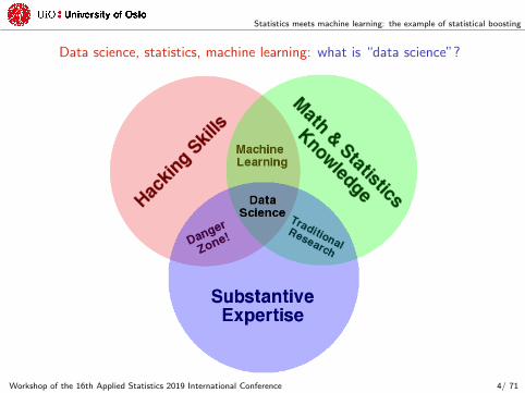
Data science, statistics, machine learning: what is “data science”?
Workshop of the 16th Applied Statistics 2019 International Conference 4/ 71
Statistics meets machine learning: the example of statistical boosting
Data science, statistics, machine learning: statistics vs machine learning
What about differences between statistics and machine learning?
‚ “Machine learning is essentially a form of applied statistics”;
‚ “Machine learning is glorified statistics”;
‚ “Machine learning is for Computer Science majors whocouldn’t pass a Statistics course”;
‚ “Machine learning is statistics scaled up to big data”;
‚ “The short answer is that there is no difference”;
Actually...
‚ “I don’t know what Machine Learning will look like in tenyears, but whatever it is I’m sure Statisticians will be whiningthat they did it earlier and better”.
(https://www.svds.com/machine-learning-vs-statistics)Workshop of the 16th Applied Statistics 2019 International Conference 5/ 71
Statistics meets machine learning: the example of statistical boosting
Data science, statistics, machine learning: statistics vs machine learning
“The difference, as we see it, is not one of algorithms or practicesbut of goals and strategies.Neither field is a subset of the other, and neither lays exclusiveclaim to a technique. They are like two pairs of old men sitting ina park playing two different board games. Both games use thesame type of board and the same set of pieces, but each plays bydifferent rules and has a different goal because the games arefundamentally different. Each pair looks at the other’s board withbemusement and thinks they’re not very good at the game.”
“Both Statistics and Machine Learning create models from data,but for different purposes.”
(https://www.svds.com/machine-learning-vs-statistics)
Workshop of the 16th Applied Statistics 2019 International Conference 6/ 71
Statistics meets machine learning: the example of statistical boosting
Data science, statistics, machine learning: statistics vs machine learning
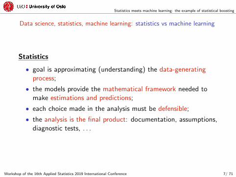
Statistics
‚ goal is approximating (understanding) the data-generatingprocess;
‚ the models provide the mathematical framework needed tomake estimations and predictions;
‚ each choice made in the analysis must be defensible;
‚ the analysis is the final product: documentation, assumptions,diagnostic tests, . . .
Workshop of the 16th Applied Statistics 2019 International Conference 7/ 71
Statistics meets machine learning: the example of statistical boosting
Data science, statistics, machine learning: statistics vs machine learning
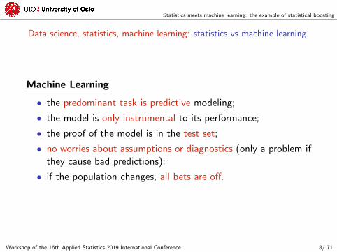
Machine Learning
‚ the predominant task is predictive modeling;
‚ the model is only instrumental to its performance;
‚ the proof of the model is in the test set;
‚ no worries about assumptions or diagnostics (only a problem ifthey cause bad predictions);
‚ if the population changes, all bets are off.
Workshop of the 16th Applied Statistics 2019 International Conference 8/ 71
Statistics meets machine learning: the example of statistical boosting
Data science, statistics, machine learning: statistics vs machine learning
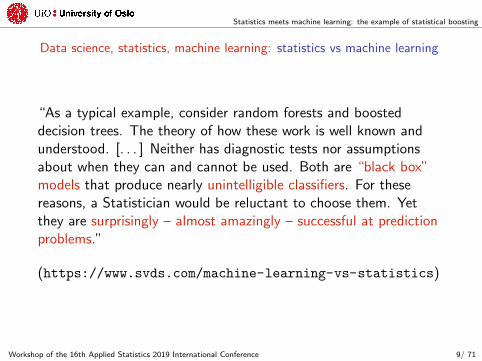
“As a typical example, consider random forests and boosteddecision trees. The theory of how these work is well known andunderstood. [. . . ] Neither has diagnostic tests nor assumptionsabout when they can and cannot be used. Both are “black box”models that produce nearly unintelligible classifiers. For thesereasons, a Statistician would be reluctant to choose them. Yetthey are surprisingly – almost amazingly – successful at predictionproblems.”
(https://www.svds.com/machine-learning-vs-statistics)
Workshop of the 16th Applied Statistics 2019 International Conference 9/ 71

Statistics meets machine learning: the example of statistical boosting
Some theory: statistical decision theory
Statistical decision theory gives a mathematical framework forfinding the optimal learner.
Let:
‚ X P IRp be a p-dimensional random vector of inputs;
‚ Y P IR be a real value random response variable;
‚ ppX,Y q be their joint distribution;
Our goal is to find a function fpXq for predicting Y given X:
‚ we need a loss function LpY, fpXqq for penalizing errors infpXq when the truth is Y ,
§ example: squared error loss, LpY, fpXqq “ pY ´ fpXqq2.
Workshop of the 16th Applied Statistics 2019 International Conference 10/ 71
Statistics meets machine learning: the example of statistical boosting
Some theory: statistical decision theory
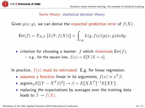
Given ppx, yq, we can derive the expected prediction error of fpXq:
Errpfq “ EX,Y rLpY, fpXqqs “
ż
x,yLpy, fpxqqppx, yqdxdy;
‚ criterion for choosing a learner: f which minimizes Errpfq;§ e.g., for the square loss, fpxq “ ErY |X “ xs.
In practice, fpxq must be estimated. E.g, for linear regression:
‚ assumes a function linear in its arguments, fpxq « xTβ;
‚ argminβErpY ´XTβq2s Ñ β “ ErXXT s´1ErXY s;
‚ replacing the expectations by averages over the training dataleads to β Ñ fpXq.
Workshop of the 16th Applied Statistics 2019 International Conference 11/ 71
Statistics meets machine learning: the example of statistical boosting
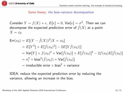
Some theory: the bias–variance decomposition
Consider Y “ fpXq ` ε, Erεs “ 0, Varrεs “ σ2. Then we candecompose the expected prediction error of fpXq at a pointX “ x0
Errpx0q “ ErpY ´ fpXqq2|X “ x0s
“ ErY 2s ` Erfpx0q2s ´ 2ErY fpx0qqs
“ VarrY s ` fpx0q2 ` Varrfpx0qs ` Erfpx0qs
2 ´ 2fpx0qErfpx0qs
“ σ2ε ` bias2pfpx0qq ` Varrfpx0qs
“ irreducible error` bias2 ` variance
IDEA: reduce the expected prediction error by reducing thevariance, allowing an increase in the bias.
Workshop of the 16th Applied Statistics 2019 International Conference 12/ 71

Statistics meets machine learning: the example of statistical boosting
Some theory: Hastie et al. (2009, Fig. 7.1)
Workshop of the 16th Applied Statistics 2019 International Conference 13/ 71
Statistics meets machine learning: the example of statistical boosting
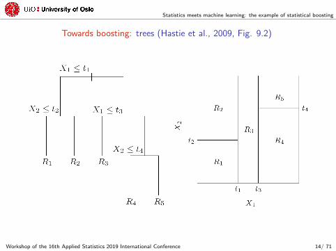
Towards boosting: trees (Hastie et al., 2009, Fig. 9.2)
Workshop of the 16th Applied Statistics 2019 International Conference 14/ 71
Statistics meets machine learning: the example of statistical boosting
Towards boosting: trees
Advantages:
‚ fast to construct, interpretable models;
‚ can incorporate mixtures of numeric and categorical inputs;
‚ immune to outliers, resistant to irrelevant inputs.
Disadvantages:
‚ lack of smoothness;
‚ difficulty in capturing additive structures;
‚ highly unstable (high variance).
Workshop of the 16th Applied Statistics 2019 International Conference 15/ 71
Statistics meets machine learning: the example of statistical boosting
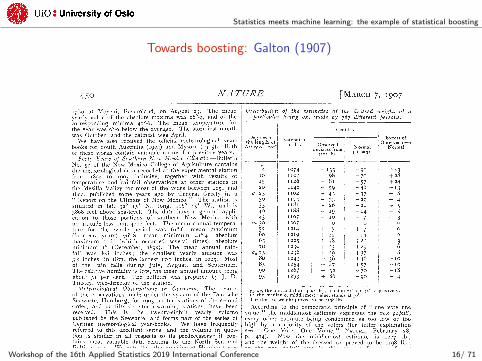
Towards boosting: Galton (1907)
© 1907 Nature Publishing Group
Workshop of the 16th Applied Statistics 2019 International Conference 16/ 71
Statistics meets machine learning: the example of statistical boosting
Towards boosting: Galton (1907)
In 1907, Sir Francis Galton visited a country fair:
A weight-judging competition was carried on at the annual show ofthe West of England Fat Stock and Poultry Exhibition recentlyheld at Plymouth. A fat ox having been selected, competitorsbought stamped and numbered cards [. . . ] on which to inscribetheir respective names, addresses, and estimates of what the oxwould weigh after it had been slaughtered and “dressed”. Thosewho guessed most successfully received prizes. About 800 ticketswere issued, which were kindly lent me for examination after theyhad fulfilled their immediate purpose.
Workshop of the 16th Applied Statistics 2019 International Conference 17/ 71
Statistics meets machine learning: the example of statistical boosting
Towards boosting: Galton (1907)
After having arrayed and analyzed the data, Galton (1907) stated:
It appears then, in this particular instance, that the vox populi iscorrect to within 1 per cent of the real value, and that theindividual estimates are abnormally distributed in such a way thatit is an equal chance whether one of them, selected at random,falls within or without the limits of -3.7 per cent and +2.4 per centof their middlemost value.
Concept of “Wisdom of Crowds” (or, as Schapire & Freund,2014, “how it is that a committee of blockheads can somehowarrive at a highly reasoned decision, despite the weak judgement ofthe individual members.”)
Workshop of the 16th Applied Statistics 2019 International Conference 18/ 71
Statistics meets machine learning: the example of statistical boosting
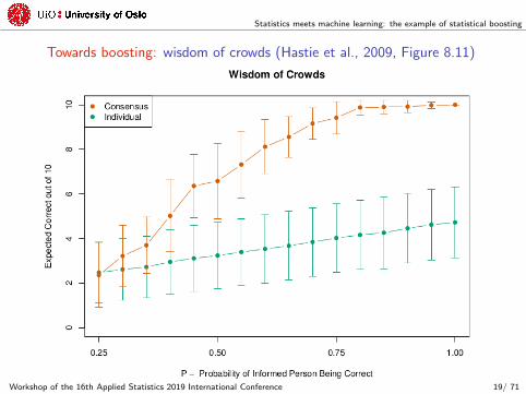
Towards boosting: wisdom of crowds (Hastie et al., 2009, Figure 8.11)
Workshop of the 16th Applied Statistics 2019 International Conference 19/ 71
Statistics meets machine learning: the example of statistical boosting
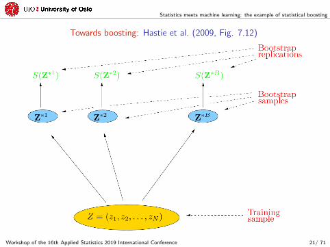
Towards boosting: translate this message into trees
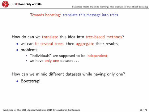
How do can we translate this idea into tree-based methods?
‚ we can fit several trees, then aggregate their results;
‚ problems:§ “individuals” are supposed to be independent;§ we have only one dataset . . .
How can we mimic different datasets while having only one?
‚ Bootstrap!
Workshop of the 16th Applied Statistics 2019 International Conference 20/ 71
Statistics meets machine learning: the example of statistical boosting
Towards boosting: Hastie et al. (2009, Fig. 7.12)
Workshop of the 16th Applied Statistics 2019 International Conference 21/ 71
Statistics meets machine learning: the example of statistical boosting
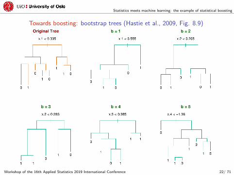
Towards boosting: bootstrap trees (Hastie et al., 2009, Fig. 8.9)
Workshop of the 16th Applied Statistics 2019 International Conference 22/ 71

Statistics meets machine learning: the example of statistical boosting
Towards boosting: bootstrap trees (Hastie et al., 2009, Fig. 8.9)
Workshop of the 16th Applied Statistics 2019 International Conference 23/ 71
Statistics meets machine learning: the example of statistical boosting
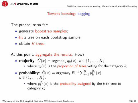
Towards boosting: bagging
The procedure so far:
‚ generate bootstrap samples;
‚ fit a tree on each bootstrap sample;
‚ obtain B trees.
At this point, aggregate the results. How?
‚ majority: Gpxq “ argmaxk qkpxq, k P t1, . . . ,Ku,§ where qkpxq is the proportion of trees voting for the category k;
‚ probability: Gpxq “ argmaxk B´1
řBb“1 p
rbsk pxq,
k P t1, . . . ,Ku,
§ where prbsk pxq is the probability assigned by the b-th tree to
category k;
Workshop of the 16th Applied Statistics 2019 International Conference 24/ 71
Statistics meets machine learning: the example of statistical boosting
Towards boosting: bagging
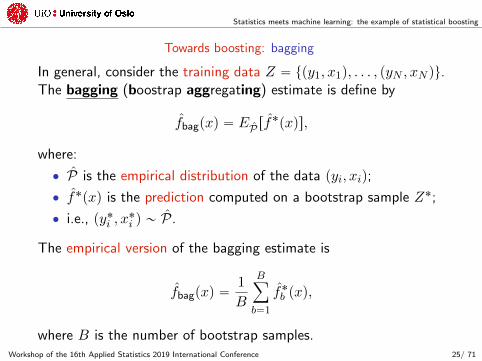
In general, consider the training data Z “ tpy1, x1q, . . . , pyN , xN qu.The bagging (boostrap aggregating) estimate is define by
fbagpxq “ EP rf˚pxqs,
where:
‚ P is the empirical distribution of the data pyi, xiq;
‚ f˚pxq is the prediction computed on a bootstrap sample Z˚;
‚ i.e., py˚i , x˚i q „ P.
The empirical version of the bagging estimate is
fbagpxq “1
B
Bÿ
b“1
f˚b pxq,
where B is the number of bootstrap samples.Workshop of the 16th Applied Statistics 2019 International Conference 25/ 71

Statistics meets machine learning: the example of statistical boosting
Towards boosting: bagging
Bagging has smaller prediction error because it reduces thevariance component,
EP rpY ´ f˚pxqq2s “ EP rpY ´ fbagpxq ` fbagpxq ´ f
˚pxqq2s
“ EP rpY ´ fbagpxqq2s ` EP rpfbagpxq ´ f
˚pxqq2s
ě EP rpY ´ fbagpxqq2s,
where P is the data distribution.
Note that this does not work for 0-1 loss:
‚ due to non-additivity of bias and variance;
‚ bagging makes better a good classifier, worse a bad one.
Workshop of the 16th Applied Statistics 2019 International Conference 26/ 71

Statistics meets machine learning: the example of statistical boosting
Towards boosting: from bagging to random forests
The average of B identically distributed r.v. with variance σ2 andpositive pairwise correlation ρ has variance
ρσ2 `1´ ρ
Bσ2.
‚ as B increases, the second term goes to 0;
‚ the bootstrap trees are p. correlated Ñ first term dominates.
Ó
construct bootstrap tree as less correlated as possible
Ó
random forests
Workshop of the 16th Applied Statistics 2019 International Conference 27/ 71
Statistics meets machine learning: the example of statistical boosting
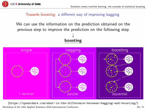
Towards boosting: a different way of improving bagging
We can use the information on the prediction obtained on theprevious step to improve the prediction on the following step
Ó
boosting
(https://quantdare.com/what-is-the-difference-between-bagging-and-boosting/)Workshop of the 16th Applied Statistics 2019 International Conference 28/ 71
Statistics meets machine learning: the example of statistical boosting
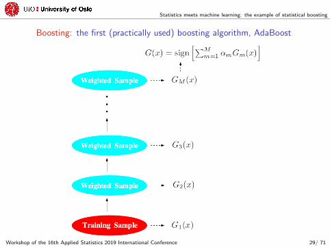
Boosting: the first (practically used) boosting algorithm, AdaBoost
Workshop of the 16th Applied Statistics 2019 International Conference 29/ 71
Statistics meets machine learning: the example of statistical boosting
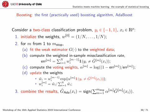
Boosting: the first (practically used) boosting algorithm, AdaBoost
Consider a two-class classification problem, yi P t´1, 1u, xi P Rp:
1. initialize the weights, wr0s “ p1{N, . . . , 1{Nq;
2. for m from 1 to mstop,
(a) fit the weak estimator Gp¨q to the weighted data;
(b) compute the weighted in-sample missclassification rate,
errrms “řNi“1 w
rm´1si 1pyi ‰ Grmspxiqq;
(c) compute the voting weights, αrms “ logpp1´ errrmsq{errrmsq;
(d) update the weights
§ wi “ wrm´1si exptαrms1pyi ‰ Grmspxiqqu;
§ wrmsi “ wi{
řNi“1 wi;
3. combine the results, GAdapxiq “ signpřmstop
m“1 αrmsGrmspxiqq.
Workshop of the 16th Applied Statistics 2019 International Conference 30/ 71
Statistics meets machine learning: the example of statistical boosting
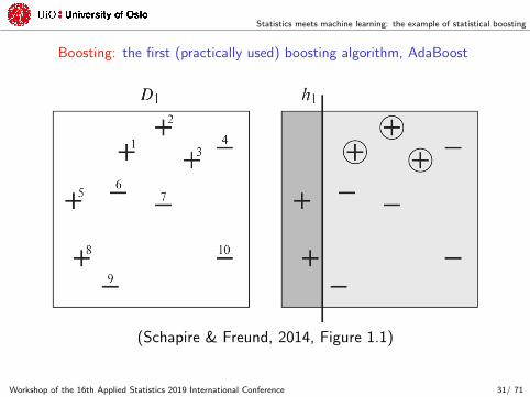
Boosting: the first (practically used) boosting algorithm, AdaBoost
(Schapire & Freund, 2014, Figure 1.1)
Workshop of the 16th Applied Statistics 2019 International Conference 31/ 71
Statistics meets machine learning: the example of statistical boosting
Boosting: the first (practically used) boosting algorithm, AdaBoost
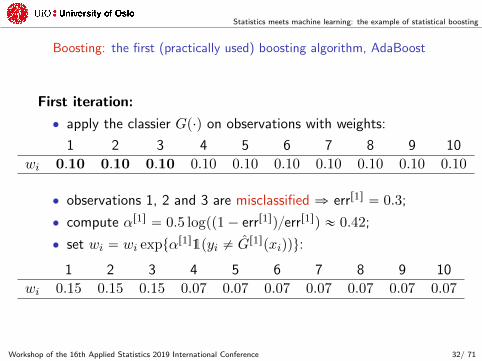
First iteration:
‚ apply the classier Gp¨q on observations with weights:
1 2 3 4 5 6 7 8 9 10
wi 0.10 0.10 0.10 0.10 0.10 0.10 0.10 0.10 0.10 0.10
‚ observations 1, 2 and 3 are misclassified ñ errr1s “ 0.3;
‚ compute αr1s “ 0.5 logpp1´ errr1sq{errr1sq « 0.42;
‚ set wi “ wi exptαr1s1pyi ‰ Gr1spxiqqu:
1 2 3 4 5 6 7 8 9 10
wi 0.15 0.15 0.15 0.07 0.07 0.07 0.07 0.07 0.07 0.07
Workshop of the 16th Applied Statistics 2019 International Conference 32/ 71

Statistics meets machine learning: the example of statistical boosting
Boosting: the first (practically used) boosting algorithm, AdaBoost
(Schapire & Freund, 2014, Figure 1.1)
Workshop of the 16th Applied Statistics 2019 International Conference 33/ 71
Statistics meets machine learning: the example of statistical boosting
Boosting: the first (practically used) boosting algorithm, AdaBoost
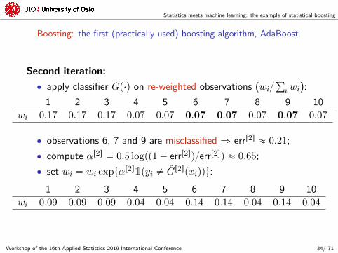
Second iteration:
‚ apply classifier Gp¨q on re-weighted observations (wi{ř
iwi):
1 2 3 4 5 6 7 8 9 10
wi 0.17 0.17 0.17 0.07 0.07 0.07 0.07 0.07 0.07 0.07
‚ observations 6, 7 and 9 are misclassified ñ errr2s « 0.21;
‚ compute αr2s “ 0.5 logpp1´ errr2sq{errr2sq « 0.65;
‚ set wi “ wi exptαr2s1pyi ‰ Gr2spxiqqu:
1 2 3 4 5 6 7 8 9 10
wi 0.09 0.09 0.09 0.04 0.04 0.14 0.14 0.04 0.14 0.04
Workshop of the 16th Applied Statistics 2019 International Conference 34/ 71
Statistics meets machine learning: the example of statistical boosting
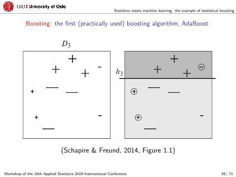
Boosting: the first (practically used) boosting algorithm, AdaBoost
(Schapire & Freund, 2014, Figure 1.1)
Workshop of the 16th Applied Statistics 2019 International Conference 35/ 71
Statistics meets machine learning: the example of statistical boosting
Boosting: the first (practically used) boosting algorithm, AdaBoost
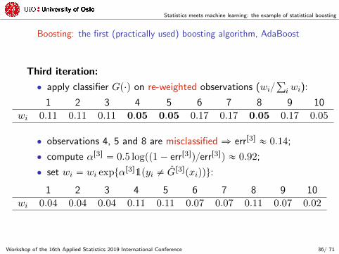
Third iteration:
‚ apply classifier Gp¨q on re-weighted observations (wi{ř
iwi):
1 2 3 4 5 6 7 8 9 10
wi 0.11 0.11 0.11 0.05 0.05 0.17 0.17 0.05 0.17 0.05
‚ observations 4, 5 and 8 are misclassified ñ errr3s « 0.14;
‚ compute αr3s “ 0.5 logpp1´ errr3sq{errr3sq « 0.92;
‚ set wi “ wi exptαr3s1pyi ‰ Gr3spxiqqu:
1 2 3 4 5 6 7 8 9 10
wi 0.04 0.04 0.04 0.11 0.11 0.07 0.07 0.11 0.07 0.02
Workshop of the 16th Applied Statistics 2019 International Conference 36/ 71

Statistics meets machine learning: the example of statistical boosting
Boosting: the first (practically used) boosting algorithm, AdaBoost
(Schapire & Freund, 2014, Figure 1.2)
Workshop of the 16th Applied Statistics 2019 International Conference 37/ 71
Statistics meets machine learning: the example of statistical boosting
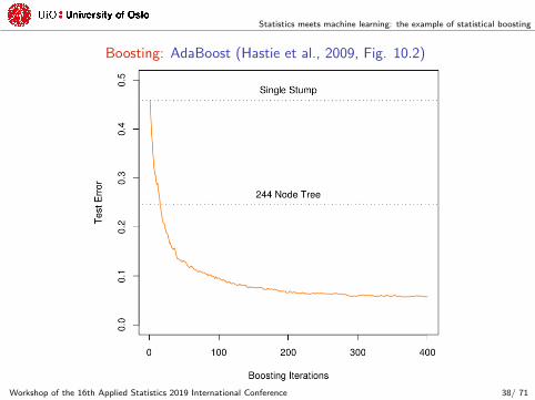
Boosting: AdaBoost (Hastie et al., 2009, Fig. 10.2)
Workshop of the 16th Applied Statistics 2019 International Conference 38/ 71

Statistics meets machine learning: the example of statistical boosting
Boosting: functional gradient descent algorithm
Friedman et al. (2000) showed that AdaBoost simply minimizes aspecific (exponential) loss function,
Lpy, fpXqq “ Ere´fpXqys,
through a functional gradient descent algorithm:
1. inizialize fpXqr0s, e.g. fpXqr0s ” 0;
2. for m “ 1, . . . ,mstop,
2.1 compute the negative gradient,
um “ ´BLpy,fpXqqBfpXq
ˇ
ˇ
ˇ
fpXq“fm´1pXq;
2.2 fit the weak estimator to the negative gradient, hmpum, Xq;
2.3 update the estimate, f rmspXq “ f rm´1spXq ` νhmpum, Xq;
3. final estimate, fboostpXq “řmstop
m“1 νhmpum, Xq.
Workshop of the 16th Applied Statistics 2019 International Conference 39/ 71
Statistics meets machine learning: the example of statistical boosting
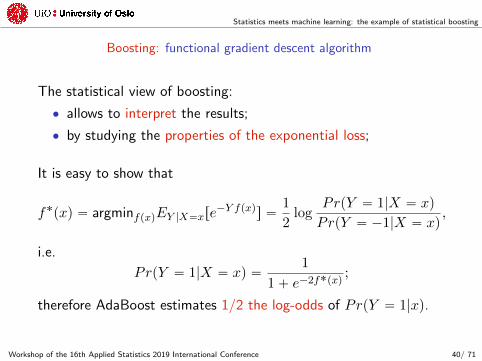
Boosting: functional gradient descent algorithm
The statistical view of boosting:
‚ allows to interpret the results;
‚ by studying the properties of the exponential loss;
It is easy to show that
f˚pxq “ argminfpxqEY |X“xre´Y fpxqs “
1
2log
PrpY “ 1|X “ xq
PrpY “ ´1|X “ xq,
i.e.
PrpY “ 1|X “ xq “1
1` e´2f˚pxq;
therefore AdaBoost estimates 1/2 the log-odds of PrpY “ 1|xq.
Workshop of the 16th Applied Statistics 2019 International Conference 40/ 71
Statistics meets machine learning: the example of statistical boosting
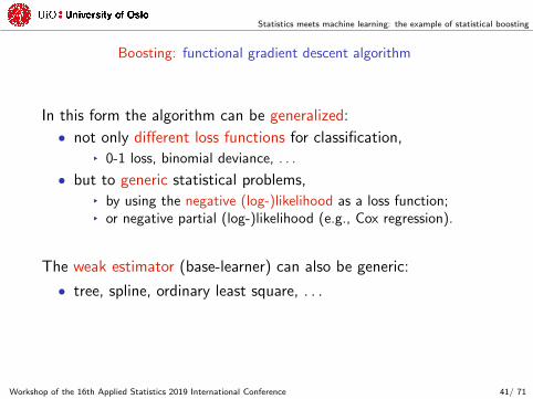
Boosting: functional gradient descent algorithm
In this form the algorithm can be generalized:
‚ not only different loss functions for classification,§ 0-1 loss, binomial deviance, . . .
‚ but to generic statistical problems,§ by using the negative (log-)likelihood as a loss function;§ or negative partial (log-)likelihood (e.g., Cox regression).
The weak estimator (base-learner) can also be generic:
‚ tree, spline, ordinary least square, . . .
Workshop of the 16th Applied Statistics 2019 International Conference 41/ 71

Statistics meets machine learning: the example of statistical boosting
Boosting: example with linear Gaussian regression
Consider the linear Gaussian regression case, with, w.l.g. y “ 0:
‚ Lpy, fpXqq “ 12
řNi“1pyi ´ fpxiqq
2;‚ hpy,Xq “ XpXTXq´1XT y.
Therefore:
‚ initialize the estimate, e.g., f0pXq “ y “ 0;‚ m “ 1,
§ u1 “ ´BLpy,fpXqqBfpXq
ˇ
ˇ
ˇ
fpXq“f0pXq“ py ´ 0q “ y;
§ h1pu1, Xq “ XpXTXq´1XT y;§ f1pxq “ 0` νXpXTXq´1XT y.
‚ m “ 2,§ u2 “ ´
BLpy,fpXqqBfpXq
ˇ
ˇ
ˇ
fpXq“f1pXq“ py ´ νXpXTXq´1XT yq;
§ h2pu2, Xq “ XpXTXq´1XT py ´ νXpXTXq´1XT yq;§ update the estimate, f2pX,βq “ νXpXTXq´1XT y `νXpXTXq´1XT py ´ νXpXTXq´1XT yq.
Workshop of the 16th Applied Statistics 2019 International Conference 42/ 71

Statistics meets machine learning: the example of statistical boosting
Statistical Boosting: Gradient boosting
Gradient boosting algorithm:
1. initialize the estimate, e.g., f0pxq “ 0;
2. for m “ 1, . . . ,mstop,
2.1 compute the negative gradient vector,
um “ ´BLpy,fpxqqBfpxq
ˇ
ˇ
ˇ
fpxq“fm´1pxq;
2.2 fit the base learner to the negative gradient vector, hmpum, xq;
2.3 update the estimate, fmpxq “ fm´1pxq ` νhmpum, xq.
3. final estimate, fmstoppxq “řmstop
m“1 νhmpum, xq
Note:
‚ X must be centered;
‚ fmstoppxq is a GAM.
Workshop of the 16th Applied Statistics 2019 International Conference 43/ 71
Statistics meets machine learning: the example of statistical boosting
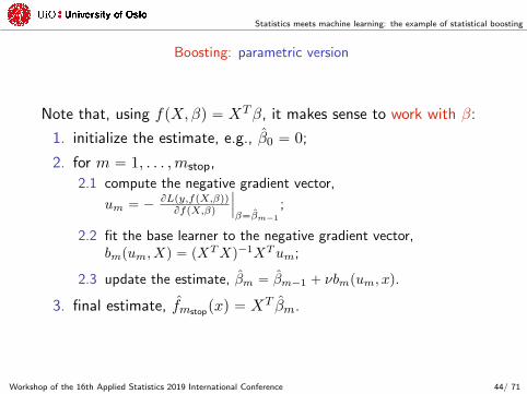
Boosting: parametric version
Note that, using fpX,βq “ XTβ, it makes sense to work with β:
1. initialize the estimate, e.g., β0 “ 0;
2. for m “ 1, . . . ,mstop,
2.1 compute the negative gradient vector,
um “ ´BLpy,fpX,βqqBfpX,βq
ˇ
ˇ
ˇ
β“βm´1
;
2.2 fit the base learner to the negative gradient vector,bmpum, Xq “ pX
TXq´1XTum;
2.3 update the estimate, βm “ βm´1 ` νbmpum, xq.
3. final estimate, fmstoppxq “ XT βm.
Workshop of the 16th Applied Statistics 2019 International Conference 44/ 71
Statistics meets machine learning: the example of statistical boosting
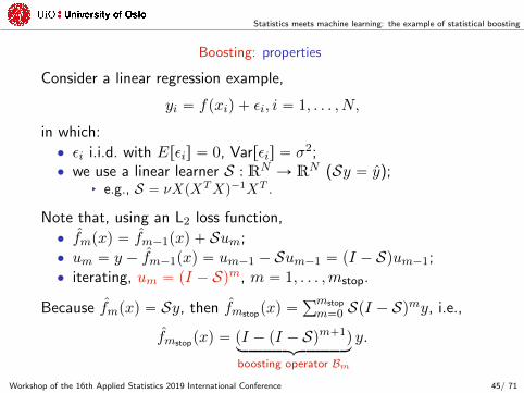
Boosting: properties
Consider a linear regression example,
yi “ fpxiq ` εi, i “ 1, . . . , N,
in which:
‚ εi i.i.d. with Erεis “ 0, Varrεis “ σ2;‚ we use a linear learner S : RN Ñ RN (Sy “ y);
§ e.g., S “ νXpXTXq´1XT .
Note that, using an L2 loss function,
‚ fmpxq “ fm´1pxq ` Sum;‚ um “ y ´ fm´1pxq “ um´1 ´ Sum´1 “ pI ´ Squm´1;‚ iterating, um “ pI ´ Sqm, m “ 1, . . . ,mstop.
Because fmpxq “ Sy, then fmstoppxq “řmstop
m“0 SpI ´ Sqmy, i.e.,
fmstoppxq “ pI ´ pI ´ Sqm`1qlooooooooomooooooooon
boosting operator Bm
y.
Workshop of the 16th Applied Statistics 2019 International Conference 45/ 71

Statistics meets machine learning: the example of statistical boosting
Boosting: properties
Consider a linear learner S (e.g., least square). Then
Proposition 1 (Buhlmann & Yu, 2003): The eigenvalues of theL2Boost operator Bm are
1´ p1´ λkqmstop`1, k “ 1, . . . , N
(
.
If S “ ST (i.e., symmetric), then Bm can be diagonalized with anorthonormal transformation,
Bm “ UDmUT , Dm “ diagp1´ p1´ λkq
mstop`1q
where UUT “ UTU “ I.
Workshop of the 16th Applied Statistics 2019 International Conference 46/ 71
Statistics meets machine learning: the example of statistical boosting
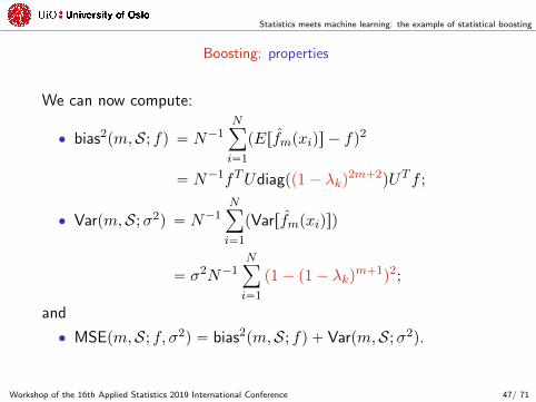
Boosting: properties
We can now compute:
‚ bias2pm,S; fq “ N´1Nÿ
i“1
pErfmpxiqs ´ fq2
“ N´1fTUdiagpp1´ λkq2m`2qUT f ;
‚ Varpm,S;σ2q “ N´1Nÿ
i“1
pVarrfmpxiqsq
“ σ2N´1Nÿ
i“1
p1´ p1´ λkqm`1q2;
and
‚ MSEpm,S; f, σ2q “ bias2pm,S; fq ` Varpm,S;σ2q.
Workshop of the 16th Applied Statistics 2019 International Conference 47/ 71
Statistics meets machine learning: the example of statistical boosting
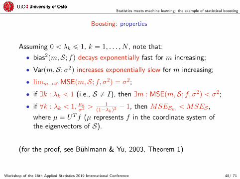
Boosting: properties
Assuming 0 ă λk ď 1, k “ 1, . . . , N , note that:
‚ bias2pm,S; fq decays exponentially fast for m increasing;
‚ Varpm,S;σ2q increases exponentially slow for m increasing;
‚ limmÑ8 MSEpm,S; f, σ2q “ σ2;
‚ if Dk : λk ă 1 (i.e., S ‰ I), then Dm : MSEpm,S; f, σ2q ă σ2;
‚ if @k : λk ă 1, µkσ2 ą
1p1´λkq2
´ 1, then MSEBm ăMSES ,
where µ “ UT f (µ represents f in the coordinate system ofthe eigenvectors of S).
(for the proof, see Buhlmann & Yu, 2003, Theorem 1)
Workshop of the 16th Applied Statistics 2019 International Conference 48/ 71

Statistics meets machine learning: the example of statistical boosting
Boosting: properties
About µkσ2 ą
1p1´λkq2
´ 1:
‚ a large left side means that f is relatively complex comparedwith the noise level σ2;
‚ a small right side means that λk is small, i.e. the learnershrinks strongly in the direction of the k-th eigenvector;
‚ therefore, to have boosting bringing improvements:§ there must be a large signal to noise ratio;§ the value of λk must be sufficiently small;
Ó
use a weak learner!!!
Workshop of the 16th Applied Statistics 2019 International Conference 49/ 71
Statistics meets machine learning: the example of statistical boosting
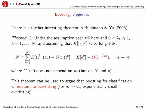
Boosting: properties
There is a further intersting theorem in Buhlmann & Yu (2003),
Theorem 2: Under the assumption seen till here and 0 ă λk ď 1,k “ 1, . . . , N , and assuming that Er|ε1|
ps ă 8 for p P N,
N´1Nÿ
i“1
Erpfmpxiq ´ fpxiqqps “ Erεp1s `Ope
´Cmq, mÑ8
where C ą 0 does not depend on m (but on N and p).
This theorem can be used to argue that boosting for classificationis resistant to overfitting (for mÑ8, exponentially smalloverfitting).
Workshop of the 16th Applied Statistics 2019 International Conference 50/ 71
Statistics meets machine learning: the example of statistical boosting
Boosting: high-dimensional settings
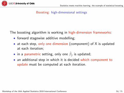
The boosting algorithm is working in high-dimension frameworks:
‚ forward stagewise additive modelling;
‚ at each step, only one dimension (component) of X is updatedat each iteration;
‚ in a parametric setting, only one βj is updated;
‚ an additional step in which it is decided which component toupdate must be computed at each iteration.
Workshop of the 16th Applied Statistics 2019 International Conference 51/ 71
Statistics meets machine learning: the example of statistical boosting
Boosting: component-wise boosting algorithm
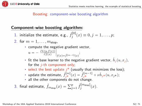
Component-wise boosting algorithm:
1. initialize the estimate, e.g., fr0sj pxq ” 0, j “ 1, . . . , p;
2. for m “ 1, . . . ,mstop,§ compute the negative gradient vector,
u “ ´ BLpy,fpxqqBfpxq
ˇ
ˇ
ˇ
fpxq“f rm´1spxq;
§ fit the base learner to the negative gradient vector, hjpu, xjq,for the j-th component only;
§ select the best update j˚ (usually that minimizes the loss);§ update the estimate, f
rmsj˚ pxq “ f
rm´1sj˚ ` νhj˚pu, xj˚q;
§ all the other componets do not change.
3. final estimate, fmstoppxq “řpj“1 f
rmstops
j pxq.
Workshop of the 16th Applied Statistics 2019 International Conference 52/ 71
Statistics meets machine learning: the example of statistical boosting
Boosting: component-wise boosting with linear learner
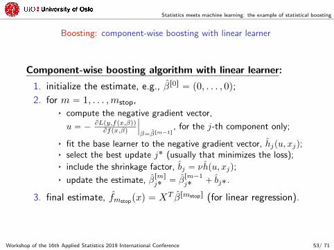
Component-wise boosting algorithm with linear learner:
1. initialize the estimate, e.g., βr0s “ p0, . . . , 0q;
2. for m “ 1, . . . ,mstop,§ compute the negative gradient vector,
u “ ´ BLpy,fpx,βqqBfpx,βq
ˇ
ˇ
ˇ
β“βrm´1s, for the j-th component only;
§ fit the base learner to the negative gradient vector, hjpu, xjq;§ select the best update j˚ (usually that minimizes the loss);§ include the shrinkage factor, bj “ νhpu, xjq;
§ update the estimate, βrmsj˚ “ β
rm´1j˚ ` bj˚ .
3. final estimate, fmstoppxq “ XT βrmstops (for linear regression).
Workshop of the 16th Applied Statistics 2019 International Conference 53/ 71

Statistics meets machine learning: the example of statistical boosting
Boosting: minimization of the loss function
β1
β 2
−250
−250
−240
−240
−230
−230
−220
−220
−210
−210
−200
−200
−190
−190
−180
−180
−170 −160
−150
−140 −130
−120
−110 −100
−90
−80
−70
−60
−50
−40
−30
−20
−10
0 1 2 3 4
01
23
4
Workshop of the 16th Applied Statistics 2019 International Conference 54/ 71
Statistics meets machine learning: the example of statistical boosting
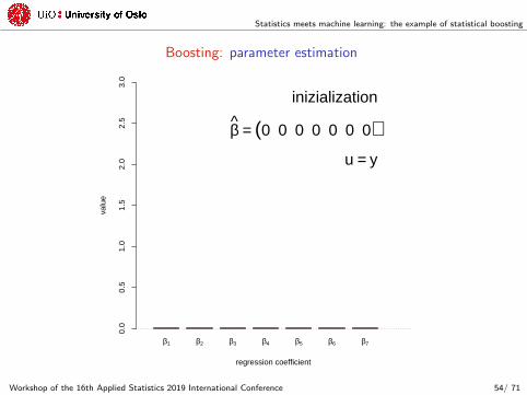
Boosting: parameter estimation
β1 β2 β3 β4 β5 β6 β7
regression coefficient
valu
e
0.0
0.5
1.0
1.5
2.0
2.5
3.0
inizialization
β = (0 0 0 0 0 0 0)u = y
Workshop of the 16th Applied Statistics 2019 International Conference 54/ 71
Statistics meets machine learning: the example of statistical boosting
Boosting: parameter estimation
β1 β2 β3 β4 β5 β6 β7
regression coefficient
valu
e
0.0
0.5
1.0
1.5
2.0
2.5
3.0
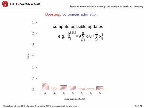
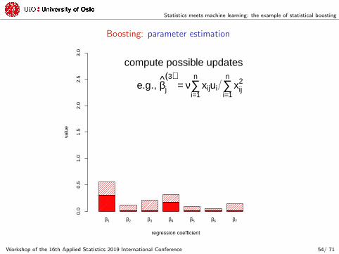
compute possible updates
e.g., βj
(1)= ν∑
i=1
nxijui ∑
i=1
nxij
2
Workshop of the 16th Applied Statistics 2019 International Conference 54/ 71
Statistics meets machine learning: the example of statistical boosting
Boosting: parameter estimation
β1 β2 β3 β4 β5 β6 β7
regression coefficient
valu
e
0.0
0.5
1.0
1.5
2.0
2.5
3.0
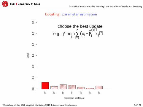
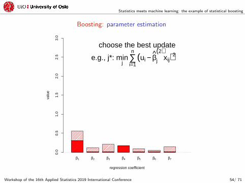
choose the best update
e.g., j*: minj
∑i=1
n(ui − βj
(1)xij)2
Workshop of the 16th Applied Statistics 2019 International Conference 54/ 71
Statistics meets machine learning: the example of statistical boosting
Boosting: parameter estimation
β1 β2 β3 β4 β5 β6 β7
regression coefficient
valu
e
0.0
0.5
1.0
1.5
2.0
2.5
3.0
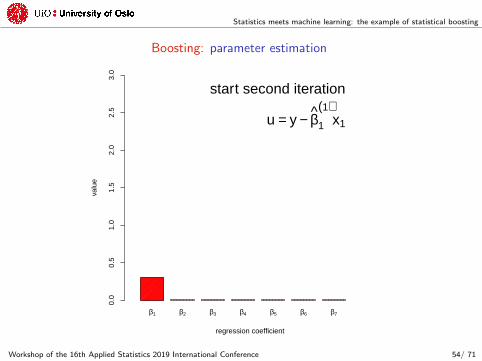
start second iteration
u = y − β1
(1)x1
Workshop of the 16th Applied Statistics 2019 International Conference 54/ 71
Statistics meets machine learning: the example of statistical boosting
Boosting: parameter estimation
β1 β2 β3 β4 β5 β6 β7
regression coefficient
valu
e
0.0
0.5
1.0
1.5
2.0
2.5
3.0
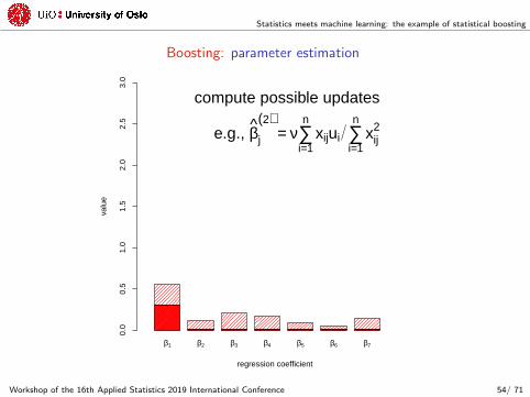
compute possible updates
e.g., βj
(2)= ν∑
i=1
nxijui ∑
i=1
nxij
2
Workshop of the 16th Applied Statistics 2019 International Conference 54/ 71
Statistics meets machine learning: the example of statistical boosting
Boosting: parameter estimation
β1 β2 β3 β4 β5 β6 β7
regression coefficient
valu
e
0.0
0.5
1.0
1.5
2.0
2.5
3.0
choose the best update
e.g., j*: minj
∑i=1
n(ui − βj
(2)xij)2
Workshop of the 16th Applied Statistics 2019 International Conference 54/ 71
Statistics meets machine learning: the example of statistical boosting
Boosting: parameter estimation
β1 β2 β3 β4 β5 β6 β7
regression coefficient
valu
e
0.0
0.5
1.0
1.5
2.0
2.5
3.0
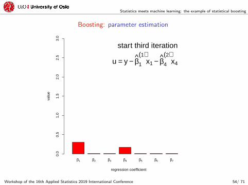
start third iteration
u = y − β1
(1)x1 − β4
(2)x4
Workshop of the 16th Applied Statistics 2019 International Conference 54/ 71
Statistics meets machine learning: the example of statistical boosting
Boosting: parameter estimation
β1 β2 β3 β4 β5 β6 β7
regression coefficient
valu
e
0.0
0.5
1.0
1.5
2.0
2.5
3.0
compute possible updates
e.g., βj
(3)= ν∑
i=1
nxijui ∑
i=1
nxij
2
Workshop of the 16th Applied Statistics 2019 International Conference 54/ 71

Statistics meets machine learning: the example of statistical boosting
Boosting: parameter estimation
β1 β2 β3 β4 β5 β6 β7
regression coefficient
valu
e
0.0
0.5
1.0
1.5
2.0
2.5
3.0
choose the best update
e.g., j*: minj
∑i=1
n(ui − βj
(3)xij)2
Workshop of the 16th Applied Statistics 2019 International Conference 54/ 71
Statistics meets machine learning: the example of statistical boosting
Boosting: parameter estimation
β1 β2 β3 β4 β5 β6 β7
regression coefficient
valu
e
0.0
0.5
1.0
1.5
2.0
2.5
3.0
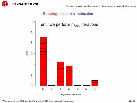
until we perform mstop iterations
Workshop of the 16th Applied Statistics 2019 International Conference 54/ 71
Statistics meets machine learning: the example of statistical boosting
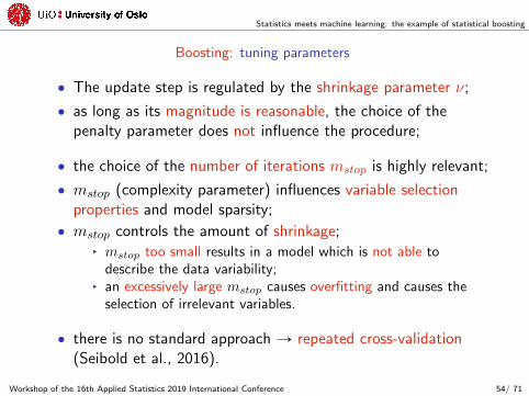
Boosting: tuning parameters
‚ The update step is regulated by the shrinkage parameter ν;
‚ as long as its magnitude is reasonable, the choice of thepenalty parameter does not influence the procedure;
‚ the choice of the number of iterations mstop is highly relevant;
‚ mstop (complexity parameter) influences variable selectionproperties and model sparsity;
‚ mstop controls the amount of shrinkage;§ mstop too small results in a model which is not able to
describe the data variability;§ an excessively large mstop causes overfitting and causes the
selection of irrelevant variables.
‚ there is no standard approach Ñ repeated cross-validation(Seibold et al., 2016).
Workshop of the 16th Applied Statistics 2019 International Conference 54/ 71
Statistics meets machine learning: the example of statistical boosting
Boosting: likelihood-based
A different version of boosting is the so-called likelihood-basedboosting (Tutz & Binder, 2006):
‚ based on the concept of GAM as well;
‚ loss function as a negative log-likelihood;
‚ uses standard statistical tools (Fisher scoring, basically aNewton-Raphson algorithm) to minimize the loss function;
‚ likelihood-based boosting and gradient boosting are equal onlyin Gaussian regression (De Bin, 2016).
Workshop of the 16th Applied Statistics 2019 International Conference 55/ 71
Statistics meets machine learning: the example of statistical boosting
Boosting: likelihood-based
The simplest implementation of the likelihood-based boosting isBoostR, based on the ridge estimator:
see also Tutz & Binder (2007).
In the rest of the lecture we will give the general idea and see itsimplementation as a special case of gradient boosting.
Workshop of the 16th Applied Statistics 2019 International Conference 56/ 71
Statistics meets machine learning: the example of statistical boosting
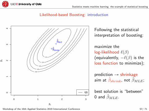
Likelihood-based Boosting: introduction
β1
β 2
−10
−20
−30
−40
−50
01
23
4
0 1 2 3
βMLE
βshrink
l(β)
Following the statisticalinterpretation of boosting:
maximize thelog-likelihood `pβq(equivalently, ´`pβq is theloss function to minimize);
prediction Ñ shrinkageaim at βshrink, not βMLE ;
best solution is “between”0 and βMLE .
Workshop of the 16th Applied Statistics 2019 International Conference 57/ 71
Statistics meets machine learning: the example of statistical boosting
Boosting: likelihood-based
β1
β 2
−10
−20
−30
−40
−50
01
23
4
0 1 2 3
βMLE
βshrink
β(0)
l(β)
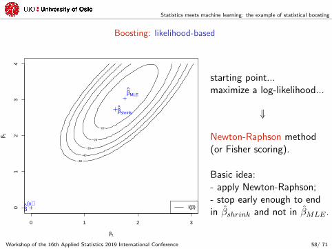
starting point...maximize a log-likelihood...
ó
Newton-Raphson method(or Fisher scoring).
Basic idea:- apply Newton-Raphson;- stop early enough to endin βshrink and not in βMLE .
Workshop of the 16th Applied Statistics 2019 International Conference 58/ 71
Statistics meets machine learning: the example of statistical boosting
Boosting: likelihood-based
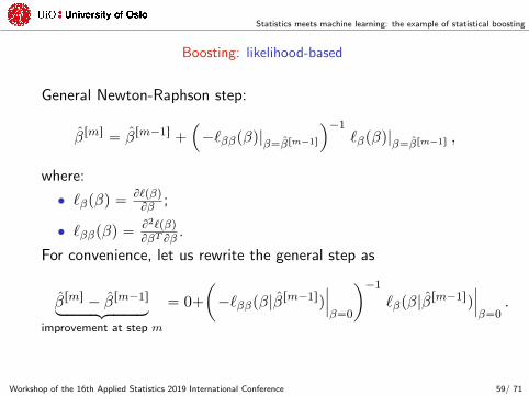
General Newton-Raphson step:
βrms “ βrm´1s `´
´`ββpβq|β“βrm´1s
¯´1`βpβq|β“βrm´1s ,
where:
‚ `βpβq “B`pβqBβ ;
‚ `ββpβq “B2`pβqBβT Bβ
.
For convenience, let us rewrite the general step as
βrms ´ βrm´1slooooooomooooooon
improvement at step m
“ 0`
ˆ
´`ββpβ|βrm´1sq
ˇ
ˇ
ˇ
β“0
˙´1
`βpβ|βrm´1sq
ˇ
ˇ
ˇ
β“0.
Workshop of the 16th Applied Statistics 2019 International Conference 59/ 71
Statistics meets machine learning: the example of statistical boosting
Boosting: likelihood-based
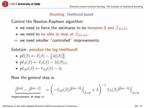
Control the Newton-Raphson algorithm:
‚ we need to force the estimates to be between 0 and βMLE ;
‚ we need to be able to stop at βshrink.
ñ we need smaller “controlled” improvements.
Solution: penalize the log-likelihood!
‚ p`pβq Ð `pβq ´ 12λ||β||
22;
‚ p`βpβq Ð `βpβq ´ λ||β||1;
‚ p`ββpβq Ð `ββpβq ´ λ;
Now the general step is:
βrms ´ βrm´1slooooooomooooooon
improvement at step m
“
ˆ
´`ββpβ|βrm´1sq
ˇ
ˇ
ˇ
β“0` λ
˙´1
`βpβ|βrm´1sq
ˇ
ˇ
ˇ
β“0
Workshop of the 16th Applied Statistics 2019 International Conference 60/ 71
Statistics meets machine learning: the example of statistical boosting
Boosting: likelihood-based
β1
β 2
−10
−20
−30
−40
−50
01
23
4
0 1 2 3
−10
−20
−30
−40
−50
β(0)
β1
(1)
β 2(1)
β(1)
−10
−20 −30 −40 −50
β1
(2)
β 2(2) β
(2)
βMLE
βshrink
l(β)
pl(β|β=β(0)
)
pl(β|β=β(1)
)boosting learning path
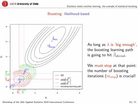
As long as λ is ‘big enough’,the boosting learning pathis going to hit βshrink.
We must stop at that point:the number of boostingiterations (mstop) is crucial!
Workshop of the 16th Applied Statistics 2019 International Conference 61/ 71
Statistics meets machine learning: the example of statistical boosting
Boosting: likelihood-based
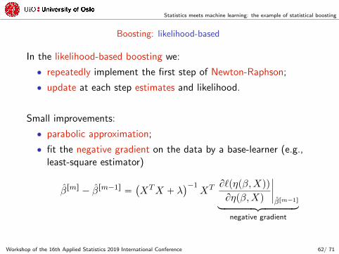
In the likelihood-based boosting we:
‚ repeatedly implement the first step of Newton-Raphson;
‚ update at each step estimates and likelihood.
Small improvements:
‚ parabolic approximation;
‚ fit the negative gradient on the data by a base-learner (e.g.,least-square estimator)
βrms ´ βrm´1s “`
XTX ` λ˘´1
XT B`pηpβ,Xqq
Bηpβ,Xq
ˇ
ˇ
ˇ
ˇ
βrm´1slooooooooooomooooooooooon
negative gradient
Workshop of the 16th Applied Statistics 2019 International Conference 62/ 71
Statistics meets machine learning: the example of statistical boosting
Boosting: likelihood-based vs gradient
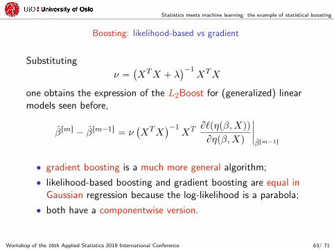
Substituting
ν “`
XTX ` λ˘´1
XTX
one obtains the expression of the L2Boost for (generalized) linearmodels seen before,
βrms ´ βrm´1s “ ν`
XTX˘´1
XT B`pηpβ,Xqq
Bηpβ,Xq
ˇ
ˇ
ˇ
ˇ
βrm´1s
‚ gradient boosting is a much more general algorithm;
‚ likelihood-based boosting and gradient boosting are equal inGaussian regression because the log-likelihood is a parabola;
‚ both have a componentwise version.
Workshop of the 16th Applied Statistics 2019 International Conference 63/ 71

Statistics meets machine learning: the example of statistical boosting
Boosting: likelihood-based vs gradient
Alternatively (more correctly) we can see the likelihood-basedboosting as a special case of the gradient boosting (De Bin, 2016):
1. initialize β “ p0, . . . , 0q;
2. for m “ 1, . . . ,mstop
§ compute the negative gradient vector, u “ B`pfpx,βqqBfpx,βq
ˇ
ˇ
ˇ
β“β§ compute the update,
bLB “
˜
Bfpx, βq
Bβ
ˇ
ˇ
ˇ
ˇ
J
β“0
u
¸
{
¨
˝´BBfpx,βqBβ
Bβ
ˇ
ˇ
ˇ
ˇ
ˇ
J
β“0
u` λ
˛
‚;
§ update the estimate, βrms “ βrm´1s ` bLB .
3. compute the final prediction, e.g., for lin. regr. y “ XT βrmstops
Workshop of the 16th Applied Statistics 2019 International Conference 64/ 71
Statistics meets machine learning: the example of statistical boosting
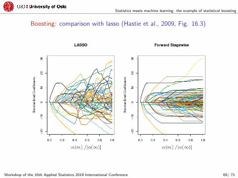
Boosting: comparison with lasso (Hastie et al., 2009, Fig. 16.3)
Workshop of the 16th Applied Statistics 2019 International Conference 65/ 71
Statistics meets machine learning: the example of statistical boosting
Boosting: back to trees
The base (weak) learner in a boosting algorithm can be a tree:
‚ largely used in practice;
‚ very powerful and fast algorithm;
‚ R package XGBoost;
‚ we lose part of the statistical interpretation.
Workshop of the 16th Applied Statistics 2019 International Conference 66/ 71
Statistics meets machine learning: the example of statistical boosting
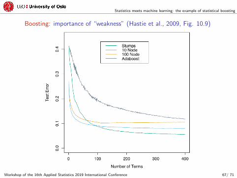
Boosting: importance of “weakness” (Hastie et al., 2009, Fig. 10.9)
Workshop of the 16th Applied Statistics 2019 International Conference 67/ 71
Statistics meets machine learning: the example of statistical boosting
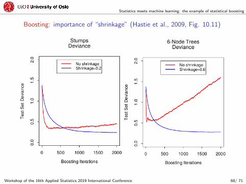
Boosting: importance of “shrinkage” (Hastie et al., 2009, Fig. 10.11)
Workshop of the 16th Applied Statistics 2019 International Conference 68/ 71
Statistics meets machine learning: the example of statistical boosting
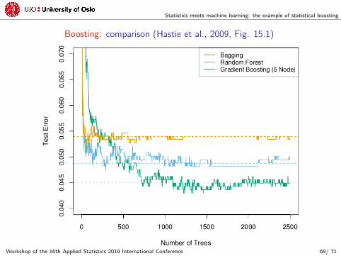
Boosting: comparison (Hastie et al., 2009, Fig. 15.1)
Workshop of the 16th Applied Statistics 2019 International Conference 69/ 71
Statistics meets machine learning: the example of statistical boosting
References I
Bhardwaj, A. (2017). What is the difference between data science andstatistics? Inhttps://priceonomics.com/whats-the-difference-between-data-science-and/.
Buhlmann, P. & Yu, B. (2003). Boosting with the L2 loss: regression andclassification. Journal of the American Statistical Association 98, 324–339.
Carmichael, I. & Marron, J. S. (2018). Data science vs. statistics: twocultures? Japanese Journal of Statistics and Data Science , 1–22.
De Bin, R. (2016). Boosting in Cox regression: a comparison between thelikelihood-based and the model-based approaches with focus on theR-packages CoxBoost and mboost. Computational Statistics 31, 513–531.
Friedman, J., Hastie, T. & Tibshirani, R. (2000). Additive logisticregression: a statistical view of boosting. The Annals of Statistics 28,337–407.
Galton, F. (1907). Vox populi. Nature 75, 450–451.
Workshop of the 16th Applied Statistics 2019 International Conference 70/ 71
Statistics meets machine learning: the example of statistical boosting
References II
Gelman, A. (2013). Statistics is the least important part of data science. Inhttp://andrewgelman.com/2013/11/14/statistics-least-important-part-data-science/.
Hastie, T., Tibshirani, R. & Friedman, J. (2009). The Elements ofStatistical Learning: Data Mining, Inference and Prediction (2nd Edition).Springer, New York.
Schapire, R. E. & Freund, Y. (2014). Boosting: Foundations andAlgorithms. MIT Press, Cambridge.
Seibold, H., Bernau, C., Boulesteix, A.-L. & De Bin, R. (2016). Onthe choice and influence of the number of boosting steps. Tech. Rep. 188,University of Munich.
Tutz, G. & Binder, H. (2006). Generalized additive modeling with implicitvariable selection by likelihood-based boosting. Biometrics 62, 961–971.
Tutz, G. & Binder, H. (2007). Boosting ridge regression. ComputationalStatistics & Data Analysis 51, 6044–6059.
Workshop of the 16th Applied Statistics 2019 International Conference 71/ 71