data analysis, statistics, machine learning
TRANSCRIPT

Data Analysis, Statistics, Machine Learning
Leland Wilkinson Adjunct Professor UIC Computer Science Chief Scien<st H2O.ai [email protected]
2
Grouping o We can create groups of variables or groups of cases o These methods involve what we call Cluster Analysis
o Hierarchical methods make trees of nested clusters o Non-‐hierarchical methods group cases into k clusters
o These k clusters may be discrete or overlapping
o Two considera<ons are especially important for hierarchical o Distance/Dissimilarity measure o Agglomera<on or spliMng rule
o The collec<on of clustering methods is huge o Early applica<ons were for numerical taxonomy in biology
Copyright © 2016 Leland Wilkinson
3
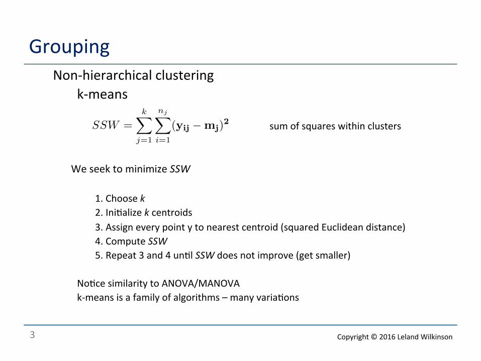
Grouping Non-‐hierarchical clustering
k-‐means o o We seek to minimize SSW
o 1. Choose k o 2. Ini<alize k centroids o 3. Assign every point y to nearest centroid (squared Euclidean distance) o 4. Compute SSW o 5. Repeat 3 and 4 un<l SSW does not improve (get smaller)
No<ce similarity to ANOVA/MANOVA k-‐means is a family of algorithms – many varia<ons
SSW =k�
j=1
nj�
i=1
(yij −mj)2 sum of squares within clusters
Copyright © 2016 Leland Wilkinson
4
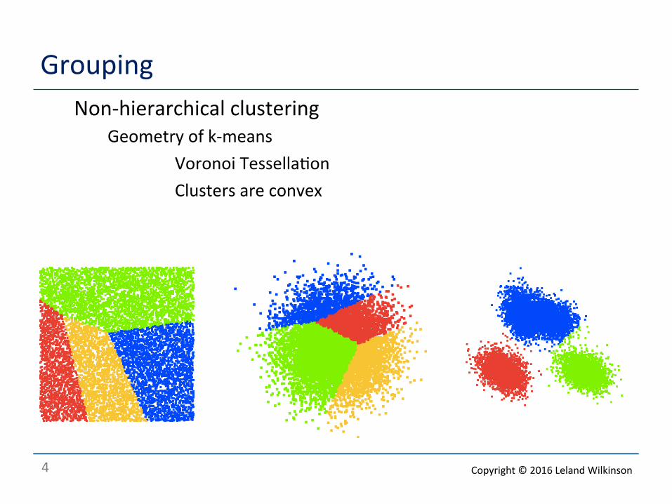
Grouping Non-‐hierarchical clustering
Geometry of k-‐means Voronoi Tessella<on Clusters are convex
o
Copyright © 2016 Leland Wilkinson
Grouping Aspects of the algorithm
Quan<za<on Even if there are no clusters, k-‐means can be used to par<<on
Detec<on of outliers Compute outliers rela<ve to cluster centroids
Clusters are convex
If a case is a weighted average of cases in the cluster, the case also lies in the cluster
k-‐means demo haps://www.cs.uic.edu/~wilkinson/Applets/cluster.html
Copyright © 2016 Leland Wilkinson 5
Grouping Non-‐hierarchical clustering
Picking k Run k-‐means from 1 to kmax Plot SSW against index and look for elbow Or, (Har<gan, 1975) SSW is distributed approximately as chi-‐square So are differences between SSWk-‐1 and SSWk Examine chi-‐square sta<s<cs for these differences (Hamerly and Elkan did something like this in 2003) They didn’t seem to be aware of Har<gan Or, compute a measure of clumpiness from minimum spanning tree (MST) Har<gan RUNT sta<s<c or Stuetzle & Nugent
Copyright © 2016 Leland Wilkinson 6
Grouping Non-‐hierarchical clustering
Picking star<ng centroids Random centroids (ugh!) Har<gan run k-‐means from 1 to k split on variable with largest variance from previous solu<on
Evalua<ng k-‐means solu<ons Can do F-‐tests on each variable (forget about p values) Can do MANOVA on groups (you’re kidding, right?) Use visualiza<on (we’ll talk about that later)
Copyright © 2016 Leland Wilkinson 7
8
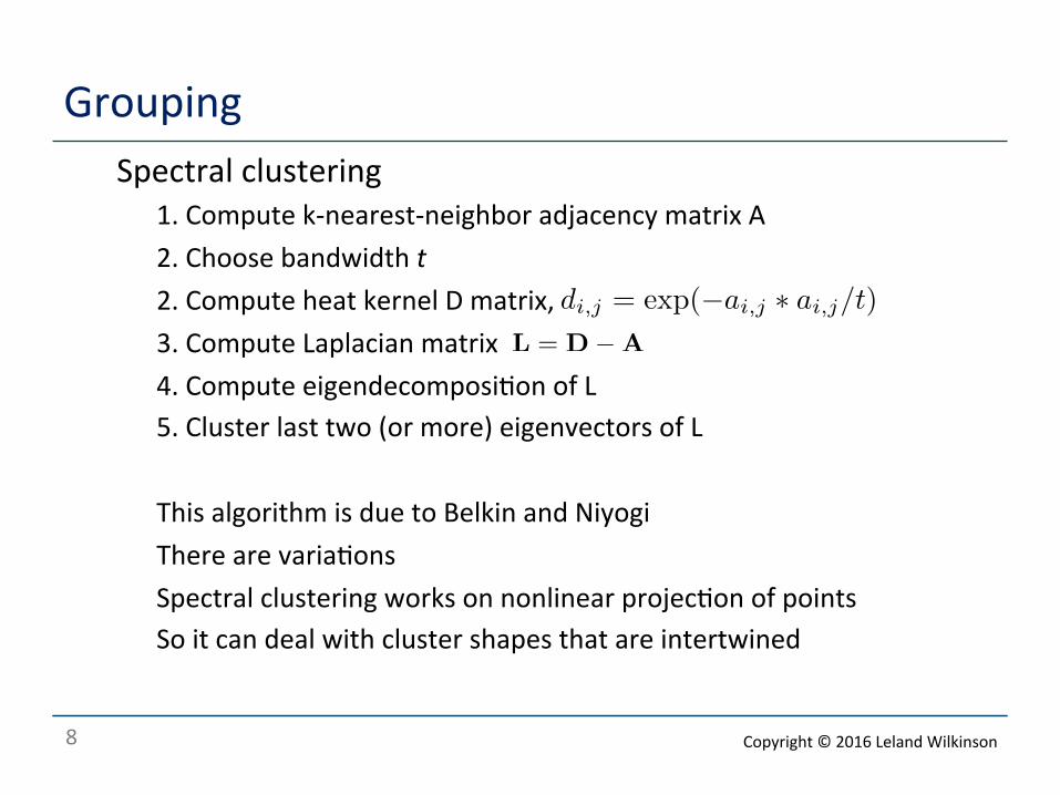
Grouping o Spectral clustering
o 1. Compute k-‐nearest-‐neighbor adjacency matrix A o 2. Choose bandwidth t o 2. Compute heat kernel D matrix, o 3. Compute Laplacian matrix o 4. Compute eigendecomposi<on of L o 5. Cluster last two (or more) eigenvectors of L o o This algorithm is due to Belkin and Niyogi o There are varia<ons o Spectral clustering works on nonlinear projec<on of points o So it can deal with cluster shapes that are intertwined
di,j = exp(−ai,j ∗ ai,j/t)L = D−A
Copyright © 2016 Leland Wilkinson
9
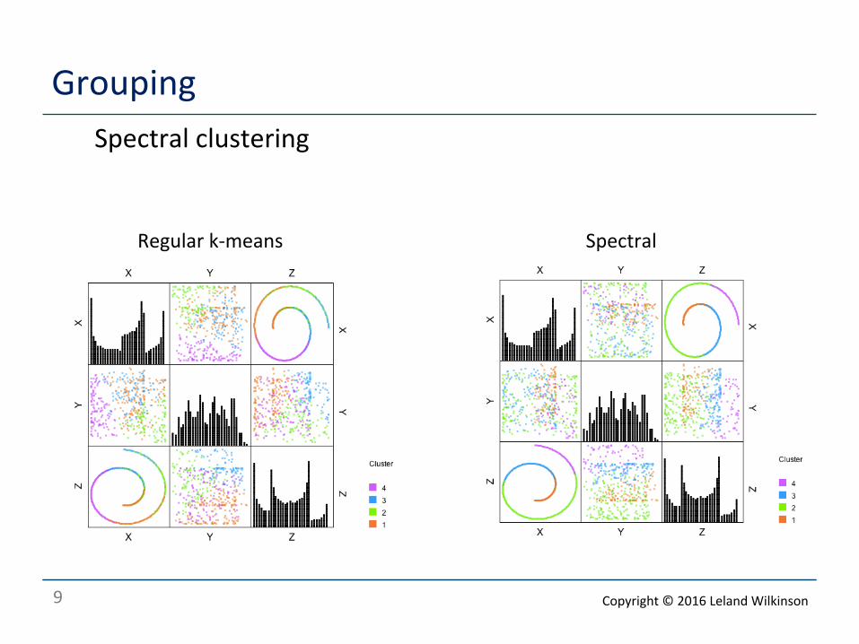
Grouping o Spectral clustering
Regular k-‐means Spectral
Copyright © 2016 Leland Wilkinson
10
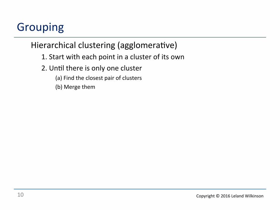
Grouping o Hierarchical clustering (agglomera<ve)
o 1. Start with each point in a cluster of its own o 2. Un<l there is only one cluster
o (a) Find the closest pair of clusters o (b) Merge them
Copyright © 2016 Leland Wilkinson
11
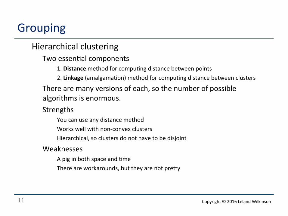
Grouping o Hierarchical clustering
o Two essen<al components o 1. Distance method for compu<ng distance between points o 2. Linkage (amalgama<on) method for compu<ng distance between clusters
o There are many versions of each, so the number of possible algorithms is enormous.
o Strengths o You can use any distance method o Works well with non-‐convex clusters o Hierarchical, so clusters do not have to be disjoint
o Weaknesses o A pig in both space and <me o There are workarounds, but they are not preay
Copyright © 2016 Leland Wilkinson
12
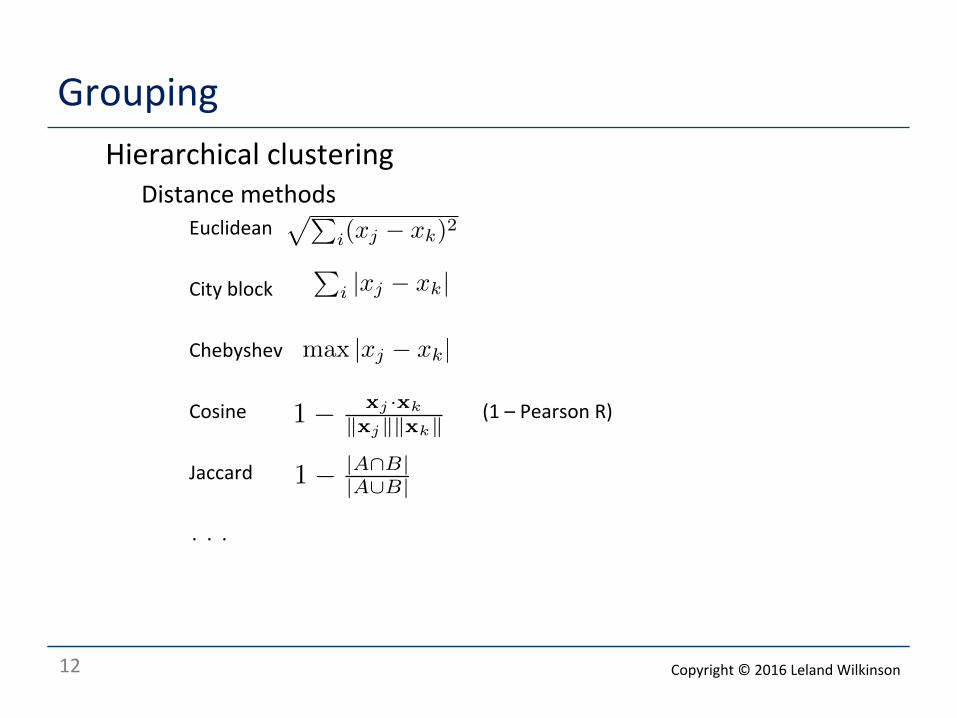
Grouping o Hierarchical clustering
o Distance methods o Euclidean
o City block
o Chebyshev
o Cosine (1 – Pearson R)
o Jaccard
. . .
��i(xj − xk)2
�i |xj − xk|
max |xj − xk|
1− xj ·xk
�xj��xk�
1− |A∩B||A∪B|
Copyright © 2016 Leland Wilkinson
13
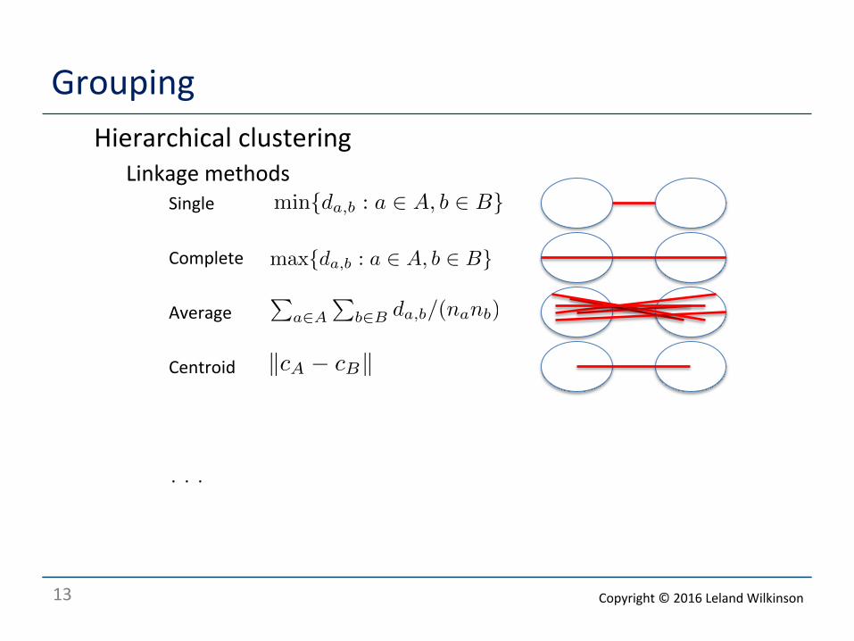
Grouping o Hierarchical clustering
o Linkage methods o Single
o Complete
o Average
o Centroid
. . .
min{da,b : a ∈ A, b ∈ B}
max{da,b : a ∈ A, b ∈ B}�
a∈A
�b∈B da,b/(nanb)
�cA − cB�
Copyright © 2016 Leland Wilkinson
14
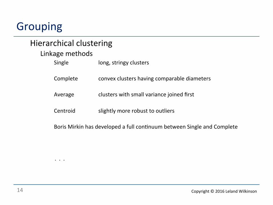
Grouping o Hierarchical clustering
o Linkage methods o Single long, stringy clusters
o Complete convex clusters having comparable diameters
o Average clusters with small variance joined first
o Centroid slightly more robust to outliers
o Boris Mirkin has developed a full con<nuum between Single and Complete
. . .
Copyright © 2016 Leland Wilkinson
15
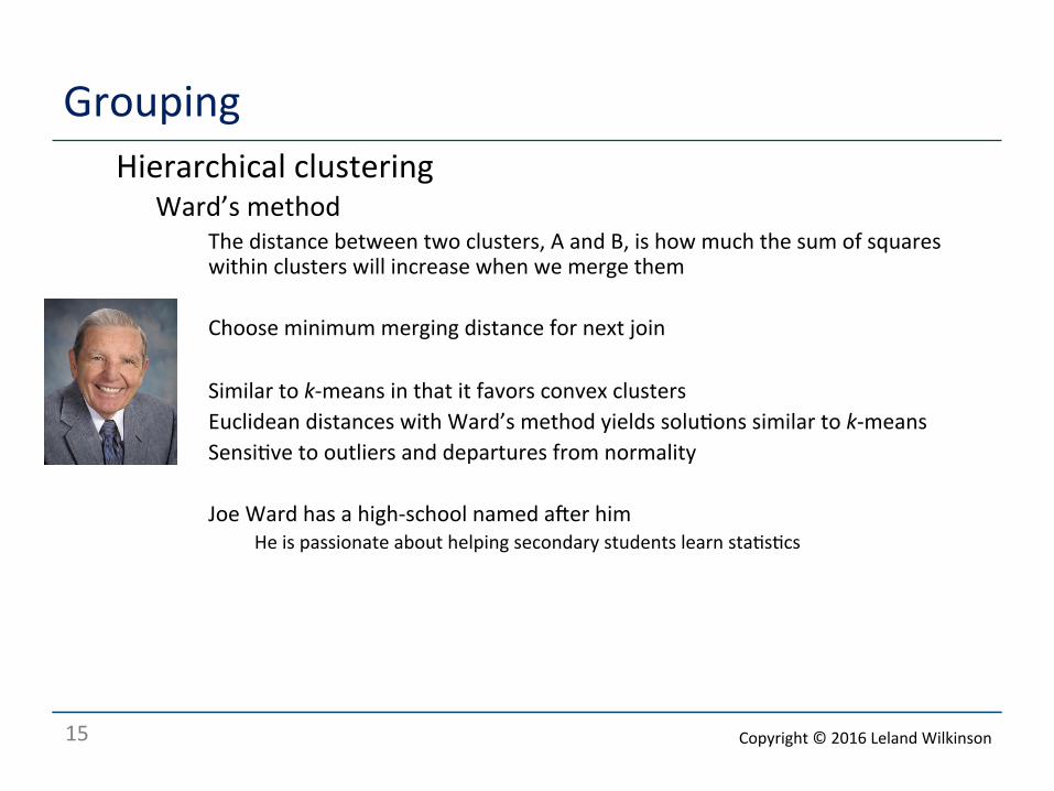
Grouping o Hierarchical clustering
o Ward’s method o The distance between two clusters, A and B, is how much the sum of squares
within clusters will increase when we merge them
o Choose minimum merging distance for next join
o Similar to k-‐means in that it favors convex clusters o Euclidean distances with Ward’s method yields solu<ons similar to k-‐means o Sensi<ve to outliers and departures from normality
o Joe Ward has a high-‐school named aqer him o He is passionate about helping secondary students learn sta<s<cs
Copyright © 2016 Leland Wilkinson
16
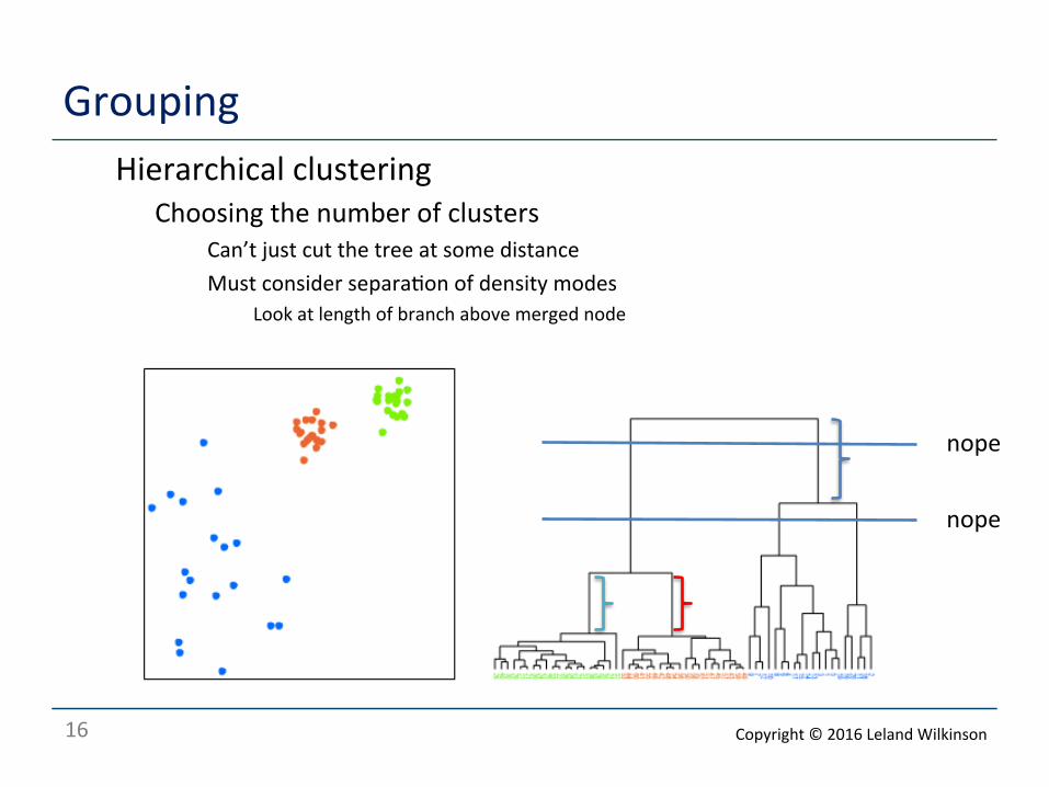
Grouping o Hierarchical clustering
o Choosing the number of clusters o Can’t just cut the tree at some distance o Must consider separa<on of density modes
o Look at length of branch above merged node
nope
nope
Copyright © 2016 Leland Wilkinson
17
Grouping o Hierarchical clustering
o Choosing the number of clusters o Can compute margin to other clusters o Silhoueae method of Rousseeuw works as well
o Includes <ghtness as well as separa<on
o Methods based on Har<gan RUNT sta<s<c work well too (Stuetzle) o Forget SS(Within) methods unless you have Gaussian clusters o Forget looking for elbow in SS plot
o You never see them with real data
Copyright © 2016 Leland Wilkinson
18
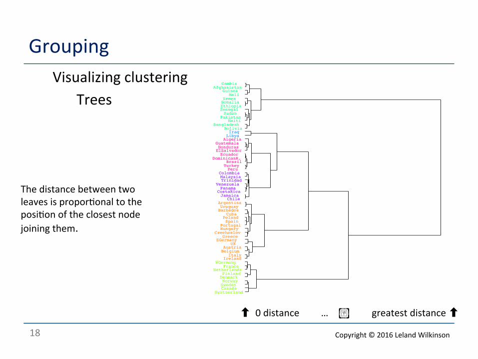
Grouping Visualizing clustering
Trees
SwitzerlandCanadaSwedenNorwayDenmarkFinland
NetherlandsFrance
WGermanyIrelandItaly
BelgiumAustria
UKEGermany
GreeceCzechoslov
HungaryPortugalSpainPolandCuba
BarbadosUruguayArgentina
ChileJamaica
CostaRicaPanama
VenezuelaTrinidadMalaysiaColombia
PeruTurkeyBrazil
DominicanR.Ecuador
ElSalvadorHondurasGuatemala
AlgeriaLibyaIraq
BoliviaBangladesh
HaitiPakistanSudan
SenegalEthiopiaSomaliaYemen
MaliGuinea
AfghanistanGambia
The distance between two leaves is propor<onal to the posi<on of the closest node joining them.
⬆ 0 distance … ︀︁︂︃︄︅︆︇︈︉︊︋︌︍︎️ greatest distance ⬆
Copyright © 2016 Leland Wilkinson
19
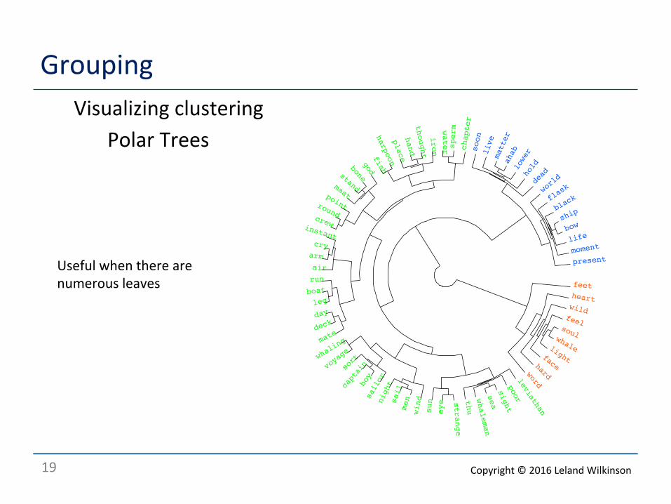
Grouping Visualizing clustering
Polar Trees
presentmomentlifebowshi
pblackfl
askwo
rldde
adholdlower
ahabmatter
live
soon
chapter
spermw
ater
iron
thought
hand
place
harpoonfish
godbonestandmastpointroundcrewinstantcry
arm
air
run
boat
leg
day
deck
mate
whaling
voyage
sort
captain
boy
sailor
night
sail
men
wind
sun
eye s
trange
thu
whaleman
sea
sightpoor
leviathan
word
hard
face
light
whale
soul
feel
wild
heart
feet
Useful when there are numerous leaves
Copyright © 2016 Leland Wilkinson
20
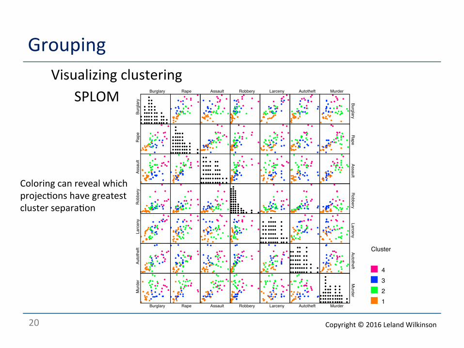
Grouping Visualizing clustering
SPLOM
Burglary
Burglary Rape Assault Robbery Larceny Autotheft Murder
Burglary
Rape Rape
Assault Assault
Robbery Robbery
Larce
ny Larceny
Autotheft
Autotheft
Burglary
Murder
Rape Assault Robbery Larceny Autotheft Murder
Murder
1234
Cluster
Coloring can reveal which projec<ons have greatest cluster separa<on
Copyright © 2016 Leland Wilkinson
21
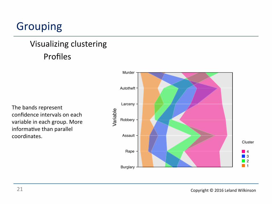
Grouping Visualizing clustering
Profiles
Burglary
Rape
Assault
Robbery
Larceny
Autotheft
Murder
Variable
1234
Cluster
The bands represent confidence intervals on each variable in each group. More informa<ve than parallel coordinates.
Copyright © 2016 Leland Wilkinson
22
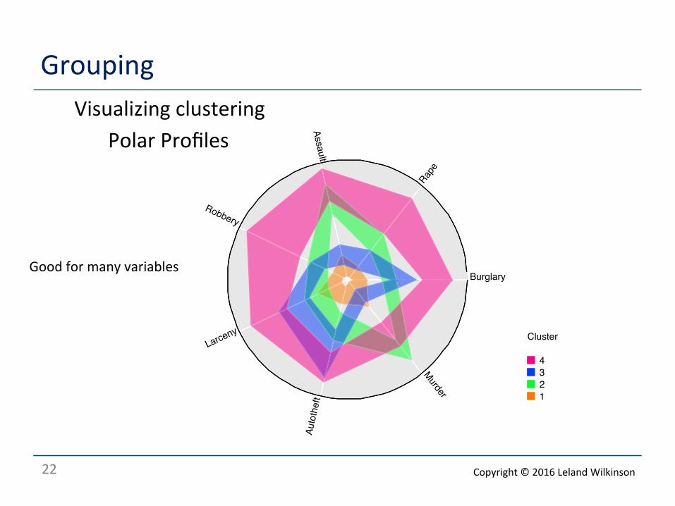
Grouping Visualizing clustering
Polar Profiles
Burglary
Rape
Assault
Robbery
Larceny
Autotheft
Murder 1234
Cluster
Good for many variables
Copyright © 2016 Leland Wilkinson
23
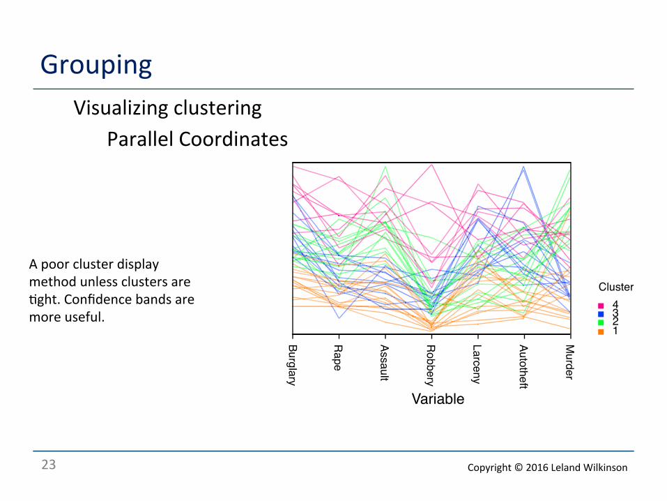
Grouping Visualizing clustering
Parallel Coordinates
Burglary
Rape
Assault
Robbery
Larceny
Autotheft
Murder
Variable
1234
ClusterA poor cluster display method unless clusters are <ght. Confidence bands are more useful.
Copyright © 2016 Leland Wilkinson
24
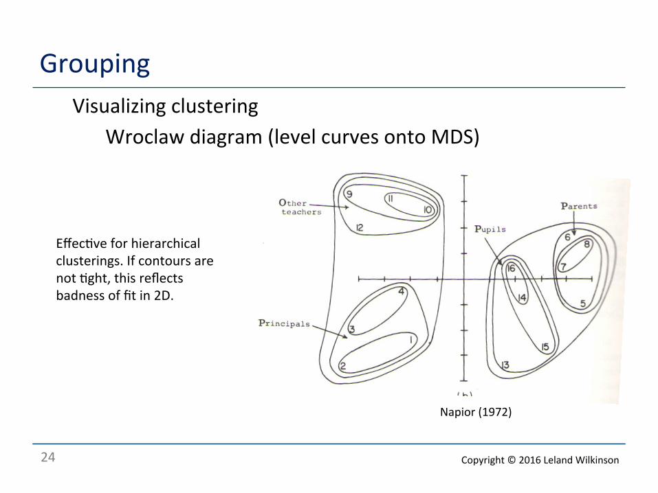
Grouping Visualizing clustering
Wroclaw diagram (level curves onto MDS)
Napior (1972)
Effec<ve for hierarchical clusterings. If contours are not <ght, this reflects badness of fit in 2D.
Copyright © 2016 Leland Wilkinson

25
Grouping Visualizing clustering
Projec<ons
-12 -6 0 6 12Component 1
-5.0
-2.5
0.0
2.5
5.0
Comp
onen
t 2
1234
cluster
-12 -6 0 6 12Component 1
-5.0
-2.5
0.0
2.5
5.0
Comp
onen
t 2
1234
cluster
-12 -6 0 6 12Component 1
-5.0
-2.5
0.0
2.5
5.0
Comp
onen
t 2
1234
cluster
-12 -6 0 6 12Component 1
-5.0
-2.5
0.0
2.5
5.0
Comp
onen
t 2
1234
cluster
Convex hulls (upper right) Alpha shapes (lower leq) Kernels (lower right) Alpha shapes are nonconvex hulls. They reveal shape of clusters beaer. Best to project these on MDS, but principal components will do OK.
Copyright © 2016 Leland Wilkinson
26
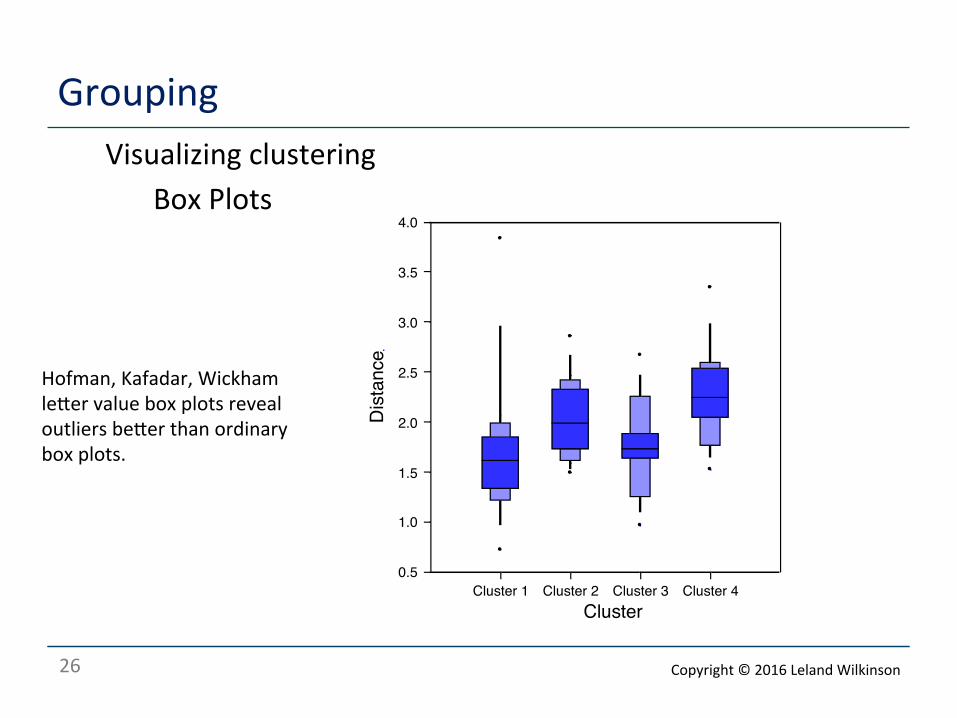
Grouping Visualizing clustering
Box Plots
Cluster 1 Cluster 2 Cluster 3 Cluster 4Cluster
0.5
1.0
1.5
2.0
2.5
3.0
3.5
4.0
Dista
nce
Hofman, Kafadar, Wickham leaer value box plots reveal outliers beaer than ordinary box plots.
Copyright © 2016 Leland Wilkinson

27
Grouping Visualizing clustering
Cluster Heatmap hap://www.datavis.ca/papers/HeatmapHistory-‐tas.2009.pdf
hsa-miR-18a hsa-miR-377 hsa-miR-147 hsa-miR-337-3p hsa-miR-212 hsa-miR-188-5p hsa-miR-141 hsa-miR-127-3p hsa-miR-381 hsa-miR-323-3p hsa-miR-299-5p hsa-miR-106a hsa-miR-382 hsa-miR-198 hsa-miR-383 hsa-miR-20a hsa-miR-376a hsa-miR-124 hsa-miR-370 hsa-miR-24-1* hsa-miR-211 hsa-miR-302b* hsa-miR-1 hsa-miR-375 hsa-miR-380* hsa-miR-219-5p hsa-miR-346 hsa-miR-92a hsa-miR-182* hsa-miR-133a hsa-miR-379 hsa-miR-326 hsa-miR-129-5p hsa-miR-203 hsa-miR-369-3p hsa-miR-208b hsa-miR-128 hsa-miR-302a* hsa-miR-154* hsa-miR-215 hsa-miR-325 hsa-miR-154 hsa-miR-194 hsa-miR-216a hsa-miR-192 hsa-miR-19b hsa-miR-19a hsa-miR-200a hsa-miR-9* hsa-miR-17 hsa-miR-200c hsa-miR-338-3p hsa-miR-136 hsa-miR-206 hsa-miR-133b hsa-miR-134 hsa-miR-17* hsa-miR-9
hsa-miR-342-3phsa-miR-208bhsa-miR-103hsa-miR-152hsa-miR-15bhsa-miR-126*hsa-miR-374ahsa-miR-370hsa-miR-203hsa-miR-200ahsa-miR-187hsa-miR-23ahsa-miR-138hsa-miR-184hsa-miR-214
hsa-miR-199b-5phsa-miR-199a-3p
hsa-miR-143hsa-miR-369-3phsa-miR-154*hsa-miR-124hsa-miR-383hsa-miR-1
hsa-miR-198hsa-miR-219-5p
hsa-miR-25hsa-miR-30ahsa-miR-182hsa-miR-125bhsa-miR-221hsa-miR-99b
hsa-let-7ehsa-miR-216ahsa-miR-93hsa-miR-136
hsa-miR-140-5phsa-miR-326hsa-miR-381hsa-miR-206hsa-miR-372
hsa-miR-371-3phsa-miR-133ahsa-miR-106bhsa-miR-182*
hsa-miR-590-5phsa-miR-100hsa-miR-29ahsa-miR-99ahsa-miR-34ahsa-miR-218hsa-miR-9
hsa-miR-30e*hsa-miR-133b
hsa-miR-125a-5phsa-miR-137hsa-miR-382hsa-miR-95hsa-miR-210hsa-miR-196b
hsa-miR-331-3phsa-miR-339-5p
hsa-miR-18ahsa-miR-134
hsa-let-7chsa-let-7b
hsa-miR-373hsa-miR-19bhsa-miR-346hsa-miR-186hsa-miR-190hsa-miR-126hsa-miR-26a
hsa-miR-28-5phsa-miR-154
hsa-miR-24-1*hsa-let-7a
hsa-miR-34c-5phsa-miR-204
hsa-miR-338-3phsa-miR-211hsa-miR-320ahsa-miR-135bhsa-miR-128hsa-miR-147hsa-miR-345hsa-miR-378*hsa-miR-135a
hsa-let-7fhsa-miR-197hsa-miR-33a
hsa-miR-181a*hsa-miR-30chsa-miR-183hsa-miR-148b
hsa-miR-423-3phsa-miR-199a-5p
hsa-miR-302bhsa-miR-10bhsa-miR-340*hsa-miR-196ahsa-miR-146ahsa-miR-155
hsa-miR-296-5phsa-miR-29bhsa-miR-10ahsa-miR-24hsa-miR-26b
hsa-miR-361-5phsa-miR-181ahsa-miR-325hsa-miR-593*hsa-miR-16hsa-miR-17*
hsa-miR-376ahsa-miR-194hsa-miR-30a*hsa-miR-367hsa-miR-153hsa-miR-222hsa-miR-379
hsa-miR-129-5phsa-miR-188-5phsa-miR-130a
hsa-miR-299-5phsa-miR-302b*hsa-miR-181b
hsa-miR-330-3phsa-miR-148ahsa-miR-30dhsa-miR-375hsa-miR-23bhsa-miR-185
hsa-miR-302a*hsa-miR-328
hsa-let-7ihsa-miR-378hsa-miR-20ahsa-miR-92ahsa-miR-98hsa-let-7g
hsa-miR-422ahsa-miR-22hsa-miR-424
hsa-miR-550a*hsa-miR-27b
hsa-miR-323-3phsa-miR-31
hsa-miR-302ahsa-miR-7hsa-let-7d
hsa-miR-17hsa-miR-193a-3p
hsa-miR-106ahsa-miR-181chsa-miR-29c
hsa-miR-127-3phsa-miR-192hsa-miR-215hsa-miR-191hsa-miR-21
hsa-miR-302dhsa-miR-30bhsa-miR-30ehsa-miR-212hsa-miR-9*
hsa-miR-200chsa-miR-141
hsa-miR-151-3phsa-miR-324-3phsa-miR-324-5phsa-miR-301ahsa-miR-15ahsa-miR-195hsa-miR-425*hsa-miR-32hsa-miR-377hsa-miR-607hsa-miR-132hsa-miR-149hsa-miR-380*hsa-miR-302chsa-miR-96hsa-miR-27ahsa-miR-130bhsa-miR-34b*hsa-miR-205hsa-miR-223hsa-miR-19ahsa-miR-150hsa-miR-107hsa-miR-145hsa-miR-335hsa-miR-101hsa-miR-224
hsa-miR-142-3phsa-miR-142-5phsa-miR-337-3p
hsa-miR-105hsa-miR-139-5p
Copyright © 2016 Leland Wilkinson
28
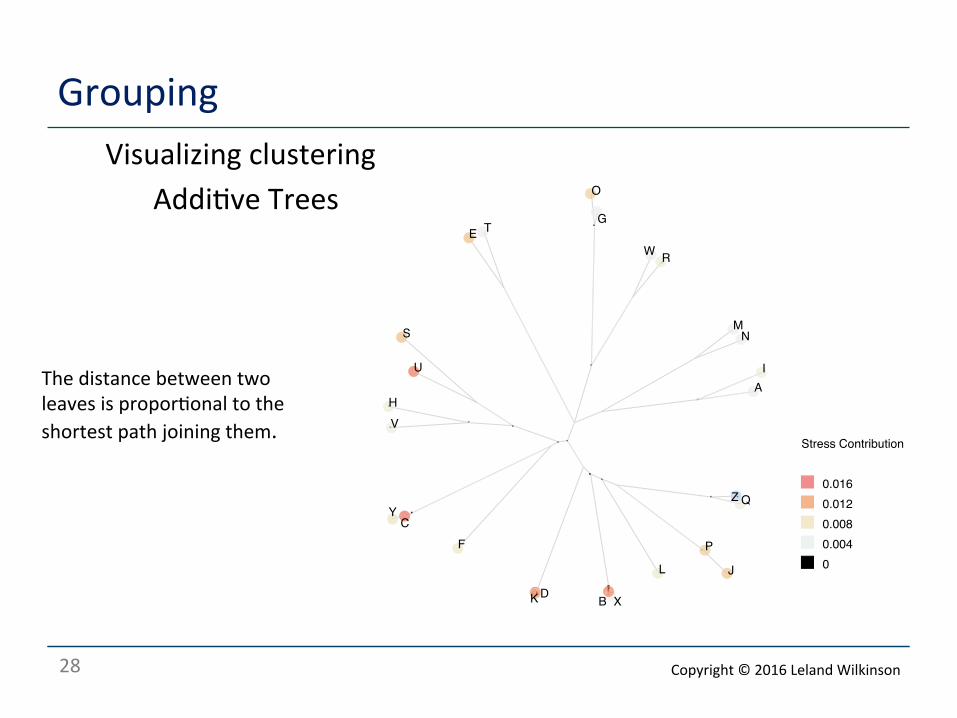
Grouping Visualizing clustering
Addi<ve Trees
D
E
F
G
A
B
C
L
MN
O
H
I
J
K
U
TW
V
Q
P
S
R
Y
X
Z
00.0040.0080.0120.016
Stress Contribution
The distance between two leaves is propor<onal to the shortest path joining them.
Copyright © 2016 Leland Wilkinson
29
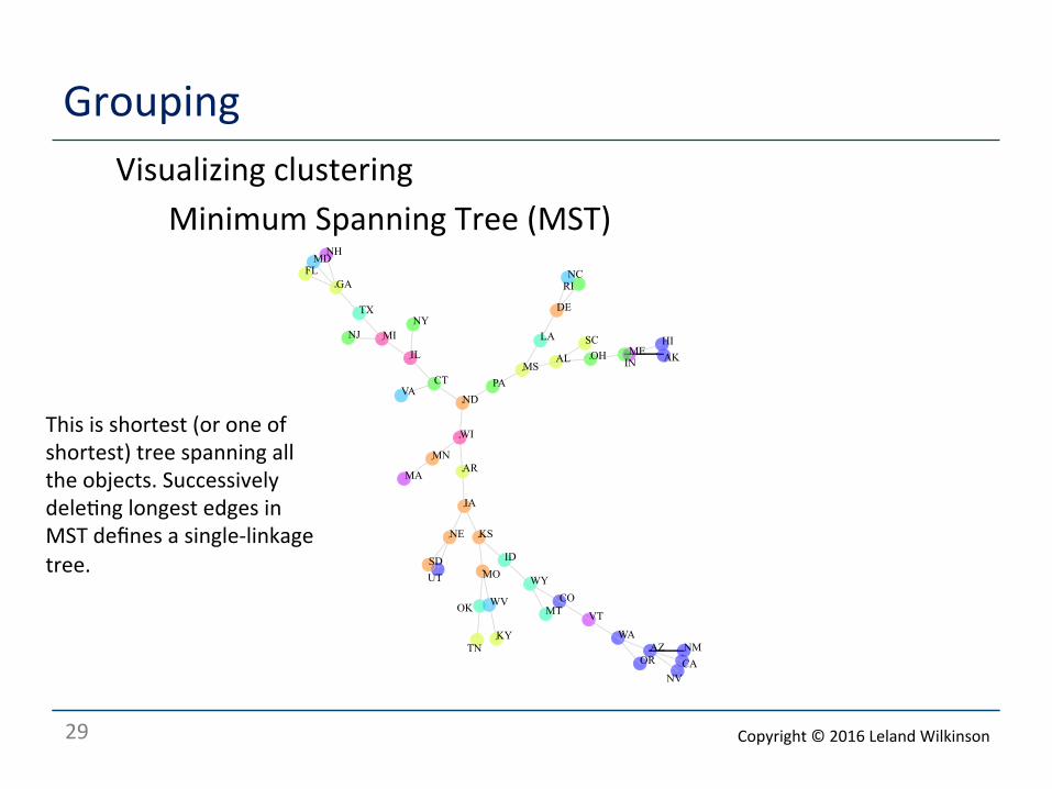
Grouping Visualizing clustering
Minimum Spanning Tree (MST)
RI
VT
HIME
VA
MI
DE
ID
IA
MD
MA AR
IL
UT
IN
MN
AZ
MO
MT
MS
NH
NJ
NM
AK
TX
AL
NC
ND
NE
NY
GA
NV
TNCA
OK
OH
WY
FL
SD
SC
CT
WV
WI
KY
KS
OR
LA
WA
CO
PA
This is shortest (or one of shortest) tree spanning all the objects. Successively dele<ng longest edges in MST defines a single-‐linkage tree.
Copyright © 2016 Leland Wilkinson

30
Grouping Visualizing clustering
Maps
12
Cluster
Drawing clusters on maps is a natural way to display geographic clusters. Clustering by state, however, can be misleading. The level of aggrega<on conceals city-‐rural differences.
Copyright © 2016 Leland Wilkinson

31
Grouping o References
o Fisher, L. and Van Ness, J.W. (1971). Admissible clustering procedures. Biometrika, 58, 91-104. o Gower, J.C. (1967). A comparison of some methods of cluster analysis. Biometrics, 23, 623-637. o Gruvaeus, G. and Wainer, H. (1972). Two additions to hierarchical cluster analysis. The British
Journal of Mathematical and Statistical Psychology, 25, 200-206. o Hartigan, J.A. (1975). Clustering algorithms. New York: John Wiley & Sons. o Hartigan, J.A., and Mohanty, S. (1992), The RUNT Test for Multi-modality, Journal of
Classification, 9, 63-70. o Johnson, S.C. (1967). Hierarchical clustering schemes. Psychometrika, 32, 241-254. o Lance, G.N., and Williams, W.T. (1967), A general theory of classificatory sorting strategies, I.
Hierarchical Systems. Computer Journal, 9, 373-380. o Milligan, G.W. (1980). An examination of the effects of six types of error perturbation on fifteen
clustering algorithms. Psychometrika, 45, 325-342. o Milligan, G.W. and Cooper, M. C. (1985). An examination of procedures for determining number of
clusters in a data set. Psychometrika, 50, 159-179. o Milligan, G.W. and Cooper, M.C. (1988). A study of standardization of variables in cluster analysis.
Journal of Classification, 45, 181-204. o Sattath, S., & Tversky, A. (1977). Additive similarity trees. Psychometrika, 42, 319-345. o Sokal, R.R. and Sneath, P.H.A. (1963). Principles of numerical taxonomy. San Francisco: W. H.
Freeman and Company. o Stuetzle, W. and Nugent, R. (2010). A generalized single linkage algorithm for estimating the cluster
tree of a density. Journal of Computational and Graphical Statistics, 19, 397-418. o Ward, J.H. (1963). Hierarchical grouping to optimize an objective function. Journal of the American
Statistical Association, 58, 236-244.
Copyright © 2016 Leland Wilkinson