statistics and probability (teaching guide)
TRANSCRIPT
TEACHING GUIDE FOR SENIOR HIGH SCHOOL
Statistics and Probability CORE SUBJECT
This Teaching Guide was collaboratively developed and reviewed by educators from public and private schools, colleges, and universities. We encourage teachers and other education
stakeholders to email their feedback, comments, and recommendations to the Commission on Higher Education, K to 12 Transition Program Management Unit - Senior High School
Support Team at [email protected]. We value your feedback and recommendations.
Commission on Higher Education in collaboration with the Philippine Normal University
INITIAL RELEASE: 13 JUNE 2016
This Teaching Guide by the Commission on Higher Education is licensed under a Creative Commons Attribution-NonCommercial-ShareAlike 4.0 International License. This means you are free to:
Share — copy and redistribute the material in any medium or format
Adapt — remix, transform, and build upon the material.
The licensor, CHED, cannot revoke these freedoms as long as you follow the license terms. However, under the following terms:
Attribution — You must give appropriate credit, provide a link to the license, and indicate if changes were made. You may do so in any reasonable manner, but not in any way that suggests the licensor endorses you or your use.
NonCommercial — You may not use the material for commercial purposes.
ShareAlike — If you remix, transform, or build upon the material, you must distribute your contributions under the same license as the original.
Printed in the Philippines by EC-TEC Commercial, No. 32 St. Louis Compound 7, Baesa, Quezon City, [email protected]
Published by the Commission on Higher Education, 2016 Chairperson: Patricia B. Licuanan, Ph.D.
Commission on Higher Education K to 12 Transition Program Management Unit Office Address: 4th Floor, Commission on Higher Education, C.P. Garcia Ave., Diliman, Quezon City Telefax: (02) 441-1143 / E-mail Address: [email protected]
DEVELOPMENT TEAM
Team Leader: Jose Ramon G. Albert, Ph.D.
Writers:Zita VJ Albacea, Ph.D., Mark John V. Ayaay
Isidoro P. David, Ph.D., Imelda E. de Mesa
Technical Editors: Nancy A. Tandang, Ph.D., Roselle V. Collado
Copy Reader: Rea Uy-Epistola
Illustrator: Michael Rey O. Santos
Cover Artists: Paolo Kurtis N. Tan, Renan U. Ortiz
CONSULTANTS THIS PROJECT WAS DEVELOPED WITH THE PHILIPPINE NORMAL UNIVERSITY.University President: Ester B. Ogena, Ph.D. VP for Academics: Ma. Antoinette C. Montealegre, Ph.D. VP for University Relations & Advancement: Rosemarievic V. Diaz, Ph.D.
Ma. Cynthia Rose B. Bautista, Ph.D., CHEDBienvenido F. Nebres, S.J., Ph.D., Ateneo de Manila University Carmela C. Oracion, Ph.D., Ateneo de Manila University Minella C. Alarcon, Ph.D., CHEDGareth Price, Sheffield Hallam University Stuart Bevins, Ph.D., Sheffield Hallam University
SENIOR HIGH SCHOOL SUPPORT TEAM CHED K TO 12 TRANSITION PROGRAM MANAGEMENT UNIT
Program Director: Karol Mark R. Yee
Lead for Senior High School Support: Gerson M. Abesamis
Lead for Policy Advocacy and Communications: Averill M. Pizarro
Course Development Officers: John Carlo P. Fernando, Danie Son D. Gonzalvo
Teacher Training Officers: Ma. Theresa C. Carlos, Mylene E. Dones
Monitoring and Evaluation Officer: Robert Adrian N. Daulat
Administrative Officers: Ma. Leana Paula B. Bato, Kevin Ross D. Nera, Allison A. Danao, Ayhen Loisse B. Dalena
IntroductionAs the Commission supports DepEd’s implementation of Senior High School (SHS), it upholds the vision and mission of the K to 12 program, stated in Section 2 of Republic Act 10533, or the Enhanced Basic Education Act of 2013, that “every graduate of basic education be an empowered individual, through a program rooted on...the competence to engage in work and be productive, the ability to coexist in fruitful harmony with local and global communities, the capability to engage in creative and critical thinking, and the capacity and willingness to transform others and oneself.”
To accomplish this, the Commission partnered with the Philippine Normal University (PNU), the National Center for Teacher Education, to develop Teaching Guides for Courses of SHS. Together with PNU, this Teaching Guide was studied and reviewed by education and pedagogy experts, and was enhanced with appropriate methodologies and strategies.
Furthermore, the Commission believes that teachers are the most important partners in attaining this goal. Incorporated in this Teaching Guide is a framework that will guide them in creating lessons and assessment tools, support them in facilitating activities and questions, and assist them towards deeper content areas and competencies. Thus, the introduction of the SHS for SHS Framework.
The SHS for SHS Framework The SHS for SHS Framework, which stands for “Saysay-Husay-Sarili for Senior High School,” is at the core of this book. The lessons, which combine high-quality content with flexible elements to accommodate diversity of teachers and environments, promote these three fundamental concepts:
SAYSAY: MEANING Why is this important?
Through this Teaching Guide, teachers will be able to facilitate an understanding of the value of the lessons, for each learner to fully engage in the content on both the cognitive and affective levels.
HUSAY: MASTERY How will I deeply understand this?
Given that developing mastery goes beyond memorization, teachers should also aim for deep understanding of the subject matter where they lead learners to analyze and synthesize knowledge.
SARILI: OWNERSHIP What can I do with this?
When teachers empower learners to take ownership of their learning, they develop independence and self-direction, learning about both the subject matter and themselves.
The Parts of the Teaching Guide This Teaching Guide is mapped and aligned to the DepEd SHS Curriculum, designed to be highly usable for teachers. It contains classroom activities and pedagogical notes, and integrated with innovative pedagogies. All of these elements are presented in the following parts:
1. INTRODUCTION • Highlight key concepts and identify the
essential questions
• Show the big picture
• Connect and/or review prerequisite knowledge
• Clearly communicate learning competencies and objectives
• Motivate through applications and connections to real-life
2. INSTRUCTION/DELIVERY • Give a demonstration/lecture/simulation/
hands-on activity
• Show step-by-step solutions to sample problems
• Use multimedia and other creative tools
• Give applications of the theory
• Connect to a real-life problem if applicable
3. PRACTICE • Discuss worked-out examples
• Provide easy-medium-hard questions
• Give time for hands-on unguided classroom work and discovery
• Use formative assessment to give feedback
4. ENRICHMENT • Provide additional examples and
applications
• Introduce extensions or generalisations of concepts
• Engage in reflection questions
• Encourage analysis through higher order thinking prompts
5. EVALUATION • Supply a diverse question bank for written
work and exercises
• Provide alternative formats for student work: written homework, journal, portfolio, group/individual projects, student-directed research project
Pedagogical Notes The teacher should strive to keep a good balance between conceptual understanding and facility in skills and techniques. Teachers are advised to be conscious of the content and performance standards and of the suggested time frame for each lesson, but flexibility in the management of the lessons is possible. Interruptions in the class schedule, or students’ poor reception or difficulty with a particular lesson, may require a teacher to extend a particular presentation or discussion.
Computations in some topics may be facilitated by the use of calculators. This is encour- aged; however, it is important that the student understands the concepts and processes involved in the calculation. Exams for the Basic Calculus course may be designed so that calculators are not necessary.
Because senior high school is a transition period for students, the latter must also be prepared for college-level academic rigor. Some topics in calculus require much more rigor and precision than topics encountered in previous mathematics courses, and treatment of the material may be different from teaching more elementary courses. The teacher is urged to be patient and careful in presenting and developing the topics. To avoid too much technical discussion, some ideas can be introduced intuitively and informally, without sacrificing rigor and correctness.
The teacher is encouraged to study the guide very well, work through the examples, and solve exercises, well in advance of the lesson. The development of calculus is one of humankind’s greatest achievements. With patience, motivation and discipline, teaching and learning calculus effectively can be realized by anyone. The teaching guide aims to be a valuable resource in this objective.
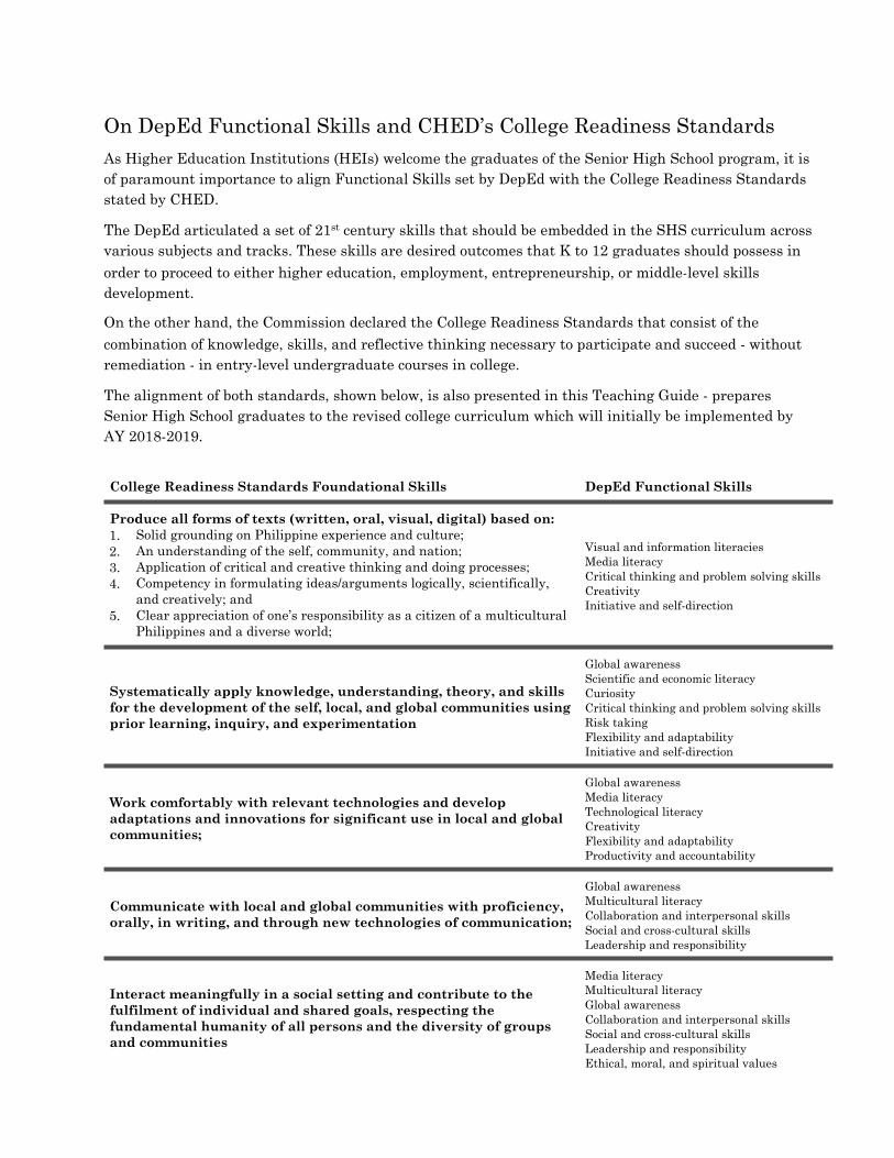
On DepEd Functional Skills and CHED’s College Readiness Standards As Higher Education Institutions (HEIs) welcome the graduates of the Senior High School program, it is of paramount importance to align Functional Skills set by DepEd with the College Readiness Standards stated by CHED.
The DepEd articulated a set of 21st century skills that should be embedded in the SHS curriculum across various subjects and tracks. These skills are desired outcomes that K to 12 graduates should possess in order to proceed to either higher education, employment, entrepreneurship, or middle-level skills development.
On the other hand, the Commission declared the College Readiness Standards that consist of the combination of knowledge, skills, and reflective thinking necessary to participate and succeed - without remediation - in entry-level undergraduate courses in college.
The alignment of both standards, shown below, is also presented in this Teaching Guide - prepares Senior High School graduates to the revised college curriculum which will initially be implemented by AY 2018-2019.
College Readiness Standards Foundational Skills DepEd Functional Skills
Produce all forms of texts (written, oral, visual, digital) based on: 1. Solid grounding on Philippine experience and culture; 2. An understanding of the self, community, and nation; 3. Application of critical and creative thinking and doing processes; 4. Competency in formulating ideas/arguments logically, scientifically,
and creatively; and 5. Clear appreciation of one’s responsibility as a citizen of a multicultural
Philippines and a diverse world;
Visual and information literacies Media literacy Critical thinking and problem solving skills Creativity Initiative and self-direction
Systematically apply knowledge, understanding, theory, and skills for the development of the self, local, and global communities using prior learning, inquiry, and experimentation
Global awareness Scientific and economic literacy Curiosity Critical thinking and problem solving skills Risk taking Flexibility and adaptability Initiative and self-direction
Work comfortably with relevant technologies and develop adaptations and innovations for significant use in local and global communities;
Global awareness Media literacy Technological literacy Creativity Flexibility and adaptability Productivity and accountability
Communicate with local and global communities with proficiency, orally, in writing, and through new technologies of communication;
Global awareness Multicultural literacy Collaboration and interpersonal skills Social and cross-cultural skills Leadership and responsibility
Interact meaningfully in a social setting and contribute to the fulfilment of individual and shared goals, respecting the fundamental humanity of all persons and the diversity of groups and communities
Media literacy Multicultural literacy Global awareness Collaboration and interpersonal skills Social and cross-cultural skills Leadership and responsibility Ethical, moral, and spiritual values
PrefacePrior to the implementation of K-12, Statistics was taught in public high schools in the Philippines typically in the last quarter of third year. In private schools, Statistics was taught as either an elective, or a required but separate subject outside of regular Math classes. In college, Statistics was taught practically to everyone either as a three unit or six unit course. All college students had to take at least three to six units of a Math course, and would typically “endure” a Statistics course to graduate. Teachers who taught these Statistics classes, whether in high school or in college, would typically be Math teachers, who may not necessarily have had formal training in Statistics. They were selected out of the understanding (or misunderstanding) that Statistics is Math. Statistics does depend on and uses a lot of Math, but so do many disciplines, e.g. engineering, physics, accounting, chemistry, computer science. But Statistics is not Math, not even a branch of Math. Hardly would one think that accounting is a branch of mathematics simply because it does a lot of calculations. An accountant would also not describe himself as a mathematician.
Math largely involves a deterministic way of thinking and the way Math is taught in schools leads learners into a deterministic way of examining the world around them. Statistics, on the other hand, is by and large dealing with uncertainty. Statistics uses inductive thinking (from specifics to generalities), while Math uses deduction (from the general to the specific).
“Statistics has its own tools and ways of thinking, and statisticians are quite insistent that those of us who teach mathematics realize that statistics is not mathematics, nor is it even a branch of mathematics. In fact, statistics is a separate discipline with its own unique ways of thinking and its own tools for approaching problems.” - J. Michael Shaughnessy, “Research on Students’ Understanding of Some Big Concepts in Statistics” (2006)
Statistics deals with data; its importance has been recognized by governments, by the private sector, and across disciplines because of the need for evidence-based decision making. It has become even more important in the past few years, now that more and more data is being collected, stored, analyzed and re-analyzed. From the time when humanity first walked the face of the earth until 2003, we created as much as 5 exabytes of data (1 exabyte being a billion “gigabytes”). Information communications technology (ICT) tools have provided us the means to transmit and exchange data much faster, whether these data are in the form of sound, text, visual images, signals or any other form or any combination of those forms using desktops, laptops, tablets, mobile phones, and other gadgets with the use of the internet, social media (facebook, twitter). With the data deluge arising from using ICT tools, as of 2012, as much as 5 exabytes were being created every two days (the amount of data created from the beginning of history up to 2003); a year later, this same amount of data was now being created every ten minutes.
In order to make sense of data, which is typically having variation and uncertainty, we need the Science of Statistics, to enable us to summarize data for describing or explaining phenomenon; or to make predictions (assuming trends in the data continue). Statistics is the science that studies data, and what we can do with data. Teachers of Statistics and Probability can easily spend much time on the formal methods and computations, losing sight of the real applications, and taking the excitement out of things. The eminent statistician Bradley Efron mentioned how diverse statistical applications are:
“During the 20th Century statistical thinking and methodology has become the scientific framework for literally dozens of fields including education, agriculture, economics, biology, and medicine, and with increasing influence recently on the hard sciences such as astronomy, geology, and physics. In other words, we have grown from a small obscure field into a big obscure field.”
In consequence, the work of a statistician has become even fashionable. Google’s chief economist Hal Varian wrote in 2009 that “the sexy job in the next ten years will be statisticians.” He went on and mentioned that “The ability to take data - to be able to understand it, to process it, to extract value from it, to visualize it, to communicate it's going to be a hugely important skill in the next decades, not only at the professional level but even at the educational level for elementary school kids, for high school kids, for college kids. “
This teaching guide, prepared by a team of professional statisticians and educators, aims to assist Senior High School teachers of the Grade 11 second semester course in Statistics and Probability so that they can help Senior High School students discover the fun in describing data, and in exploring the stories behind the data. The K-12 curriculum provides for concepts in Statistics and Probability to be taught from Grade 1 up to Grade 8, and in Grade 10, but the depth at which learners absorb these concepts may need reinforcement. Thus, the first chapter of this guide discusses basic tools (such as summary measures and graphs) for describing data. While Probability may have been discussed prior to Grade 11, it is also discussed in Chapter 2, as a prelude to defining Random Variables and their Distributions. The next chapter discusses Sampling and Sampling Distributions, which bridges Descriptive Statistics and Inferential Statistics. The latter is started in Chapter 4, in Estimation, and further discussed in Chapter 5 (which deals with Tests of Hypothesis). The final chapter discusses Regression and Correlation.
Although Statistics and Probability may be tangential to the primary training of many if not all Senior High School teachers of Statistics and Probability, it will be of benefit for them to see why this course is important to teach. After all, if the teachers themselves do not find meaning in the course, neither will the students. Work developing this set of teaching materials has been supported by the Commission on Higher Education under a Materials Development Sub-project of the K-12 Transition Project. These materials will also be shared with Department of Education.
Writers of this teaching guide recognize that few Senior High School teachers would have formal training or applied experience with statistical concepts. Thus, the guide gives concrete suggestions on classroom activities that can illustrate the wide range of processes behind data collection and data analysis.
It would be ideal to use technology (i.e. computers) as a means to help teachers and students with computations; hence, the guide also provides suggestions in case the class may have access to a computer room (particularly the use of spreadsheet applications like Microsoft Excel). It would be unproductive for teachers and students to spend too much time working on formulas, and checking computation errors at the expense of gaining knowledge and insights about the concepts behind the formulas.
The guide gives a mixture of lectures and activities, (the latter include actual collection and analysis of data). It tries to follow suggestions of the Guidelines for Assessment and Instruction in Statistics Education (GAISE) Project of the American Statistical Association to go beyond lecture methods, and instead exercise conceptual learning, use active learning strategies and focus on real data. The guide suggests what material is optional as there is really a lot of material that could be taught, but too little time. Teachers will have to find a way of recognizing that diverse needs of students with variable abilities and interests.
This teaching guide for Statistics and Probability, to be made available both digitally and in print to senior high school teachers, shall provide Senior High School teachers of Statistics and Probability with much-needed support as the country’s basic education system transitions into the K-12 curriculum. It is earnestly hoped that Senior High School teachers of Grade 11 Statistics and Probability can direct students into examining the context of data, identifying the consequences and implications of stories behind Statistics and Probability, thus becoming critical consumers of information. It is further hoped that the competencies gained by students in this course will help them become more statistical literate, and more prepared for whatever employment choices (and higher education specializations) given that employers are recognizing the importance of having their employee know skills on data management and analysis in this very data-centric world.
C h a p t e r ( 1 : ( E x p l o r i n g ( D a t a ( – ( L e s s o n ( 1 ( Page(1((
Chapter 1: Exploring Data Lesson 1: Introducing Statistics TIME FRAME:1 hour session
OVERVIEW OF LESSON
In decision making, we use statistics although some of us may not be aware of it. In this lesson, we make the students realize that to decide logically, they need to use statistics. An inquiry could be answered or a problem could be solved through the use of statistics. In fact, without knowing it we use statistics in our daily activities.
LEARNING COMPETENCIES: At the end of the lesson, the learner should be able to identify questions that could be answered using a statistical process and describe the activities involved in a statistical process.
LESSON OUTLINE:
1. Motivation 2. Statistics as a Tool in Decision-Making 3. Statistical Process in Solving a Problem
DEVELOPMENT OF THE LESSON
A. Motivation
You may ask the students, a question that is in their mind at that moment. You may write their answers on the board. (Note: You may try to group the questions as you write them on the board into two, one group will be questions that are answerable by a fact and the other group are those that require more than one information and needs further thinking).
The following are examples of what you could have written on the board:
Group 1: • How old is our teacher? • Is the vehicle of the Mayor of our city/town/municipality bigger than the vehicle used by
the President of the Philippines? • How many days are there in December? • Does the Principal of the school has a post graduate degree? • How much does the Barangay Captain receive as allowance? • What is the weight of my smallest classmate?
Group 2: • How old are the people residing in our town?
C h a p t e r ( 1 : ( E x p l o r i n g ( D a t a ( – ( L e s s o n ( 1 ( Page(2((
• Do dogs eat more than cats? • Does it rain more in our country than in Thailand? • Do math teachers earn more than science teachers? • How many books do my classmates usually bring to school? • What is the proportion of Filipino children aged 0 to 5 years who are underweight or
overweight for their age?
The first group of questions could be answered by a piece of information which is considered always true. There is a correct answer which is based on a fact and you don’t need the process of inquiry to answer such kind of question. For example, there is one and only one correct answer to the first question in Group 1 and that is your age as of your last birthday or the number of years since your birth year. On the other hand, in the second group of questions one needs observations or data to be able to respond to the question. In some questions you need to get the observations or responses of all those concerned to be able to answer the question. On the first question in the second group, you need to ask all the people in the locality about their age and among the values you obtained you get a representative value. To answer the second question in the second group, you need to get the amount of food that all dogs and cats eat to respond to the question. However, we know that is not feasible to do so. Thus what you can do is get a representative group of dogs and another representative group for the cats. Then we measure the amount of food each group of animal eats. From these two sets of values, we could then infer whether dogs do eat more than cats. So as you can see in the second group of questions you need more information or data to be able to answer the question. Either you need to get observations from all those concerned or you get representative groups from which you gather your data. But in both cases, you need data to be able to respond to the question. Using data to find an answer or a solution to a problem or an inquiry is actually using the statistical process or doing it with statistics. Now, let us formalize what we discussed and know more about statistics and how we use it in decision-making. B. Main Lesson
1. Statistics as a Tool in Decision-Making
Statistics is defined as a science that studies data to be able to make a decision. Hence, it is a tool in decision-making process. Mention that Statistics as a science involves the methods of collecting, processing, summarizing and analyzing data in order to provide answers or solutions to an inquiry. One also needs to interpret and communicate the results of the methods identified above to support a decision that one makes when faced with a problem or an inquiry.
Trivia: The word “statistics” actually comes from the word “state”— because governments have been involved in the statistical activities, especially the conduct of censuses either for military or taxation purposes. The need for and conduct of censuses are recorded in the pages of holy texts. In the Christian Bible, particularly the Book of Numbers, God is reported to have instructed Moses to carry out a census. Another census mentioned in the
C h a p t e r ( 1 : ( E x p l o r i n g ( D a t a ( – ( L e s s o n ( 1 ( Page(3((
Bible is the census ordered by Caesar Augustus throughout the entire Roman Empire before the birth of Christ.
Inform students that uncovering patterns in data involves not just science but it is also an art, and this is why some people may think “Stat is eeeks!” and may view any statistical procedures and results with much skepticism. (See Figure 1-1.)
Make known to students that Statistics enable us to • characterize persons, objects, situations, and phenomena; • explain relationships among variables; • formulate objective assessments and comparisons; and, more importantly • make evidence-based decisions and predictions.
And to use Statistics in decision-making there is a statistical process to follow which is to be discussed in the next section.
2. Statistical Process in Solving a Problem
You may go back to one of the questions identified in the second group and use it to discuss the components of a statistical process. For illustration on how to do it, let us discuss how we could answer the question “Do dogs eat more than cats?”
As discussed earlier, this question requires you to gather data to generate statistics which will serve as basis in answering the query. There should be plan or a design on how to collect the data so that the information we get from it is enough or sufficient for us to minimize any bias in responding to the query. In relation to the query, we said earlier that we cannot gather the data from all dogs and cats. Hence, the plan is to get representative group of dogs and another representative group of cats. These representative groups were observed for some characteristics like the animal weight, amount of food in grams eaten per day and breed of the animal. Included in the plan are factors like how many dogs and cats are included in the group, how to select those included in the representative groups and when to observe these animals for their characteristics.
After the data were gathered, we must verify the quality of the data to make a good decision. Data quality check could be done as we process the data to summarize the information extracted from the data. Then using this information, one can then make a decision or provide answers to the problem or question at hand.
To summarize, a statistical process in making a decision or providing solutions to a problem include the following:
• Planning or designing the collection of data to answer statistical questions in a way that maximizes information content and minimizes bias;
• Collecting the data as required in the plan; • Verifying the quality of the data after they were collected; • Summarizing the information extracted from the data; and • Examining the summary statistics so that insight and meaningful information can be
produced to support decision-making or solutions to the question or problem at hand.
C h a p t e r ( 1 : ( E x p l o r i n g ( D a t a ( – ( L e s s o n ( 1 ( Page(4((
Hence, several activities make up a statistical process which for some the process is simple but for others it might be a little bit complicated to implement. Also, not all questions or problems could be answered by a simple statistical process. There are indeed problems that need complex statistical process. However, one can be assured that logical decisions or solutions could be formulated using a statistical process.
KEY POINTS • Difference between questions that could be and those that could not answered using
Statistics. • Statistics is a science that studies data. • There are many uses of Statistics but its main use is in decision-making. • Logical decisions or solutions to a problem could be attained through a statistical process.
REFERENCES
Albert, J. R. G. (2008).Basic Statistics for the Tertiary Level (ed. Roberto Padua, Welfredo Patungan, Nelia Marquez), published by Rex Bookstore.
Handbook of Statistics 1 (1st and 2nd Edition), Authored by the Faculty of the Institute of Statistics, UP Los Baños, College Laguna 4031
Workbooks in Statistics 1 (From 1st to 13th Edition), Authored by the Faculty of the Institute of Statistics, UP Los Baños, College Laguna 4031
https://www.illustrativemathematics.org/content-standards/tasks/703
http://www.cartoonstock.com
ASSESSMENT Note: Answers are provided inside the parentheses and in bold face.
1. Identify which of the following questions are answerable using a statistical process. a. What is a typical size of a Filipino family? (answerable through a statistical process) b. How many hours in a day? (not answerable through a statistical process) c. How old is the oldest man residing in the Philippines? (answerable through a
statistical process) d. Is planet Mars bigger than planet Earth? (not answerable through a statistical
process) e. What is the average wage rate in the country? (answerable through a statistical
process) f. Would Filipinos prefer eating bananas rather than apple? (answerable through a
statistical process) g. How long did you sleep last night? (not answerable through a statistical process)
C h a p t e r ( 1 : ( E x p l o r i n g ( D a t a ( – ( L e s s o n ( 1 ( Page(5((
h. How much a newly-hired public school teacher in NCR earns in a month? (not answerable through a statistical process)
i. How tall is a typical Filipino? (answerable through a statistical process) j. Did you eat your breakfast today? (not answerable through a statistical process)
2. For each of the identified questions in Number 1 that are answerable using a statistical
process, describe the activities involved in the process.
For a. What is a typical size of a Filipino family? (The process includes getting a representative group of Filipino families and ask the family head as to how many members do they have in their family. From the gathered data which had undergone a quality check a typical value of the number of family members could be obtained. Such typical value represents a possible answer to the question.)
For c. How old is the oldest man residing in the Philippines? (The process includes getting the ages of all residents of the country. From the gathered data which had undergone a quality check the highest value of age could be obtained. Such value is the answer to the question.)
For e. What is the average wage rate in the country? (The process includes getting all prevailing wage rates in the country. From the gathered data which had undergone a quality check a typical value of the wage rate could be obtained. Such value is the answer to the question.)
For f. Would Filipinos prefer eating bananas rather than apple? (The process includes getting a representative group of Filipinos and ask each one of them on what fruit he/she prefers, banana or apple? From the gathered data which had undergone a quality check the proportion of those who prefers banana and proportion of those who prefer apple will be computed and compared. The results of this comparison could provide a possible answer to the question.)
For i. How tall is a typical Filipino? (The process includes getting a representative group of Filipinos and measure the height of each member of the representative group. From the gathered data which had undergone a quality check a typical value of the height of a Filipino could be obtained. Such typical value represents a possible answer to the question.)
Note: Tell the students that getting a representative group and obtaining a typical value are to be learned in subsequent lessons in this subject.
C h a p t e r ( 1 ( E x p l o r i n g ( D a t a ( – ( L e s s o n ( 2 ( Page(1((
Chapter 1: Exploring Data Lesson 2: Data Collection Activity TIME FRAME:1 hour session
OVERVIEW OF LESSON
As we have learned in the previous lesson, Statistics is a science that studies data. Hence to teach Statistics, real data set is recommend to use. In this lesson,we present an activity where the students will be asked to provide some data that will be submitted for consolidation by the teacher for future lessons. Data on heights and weights, for instance, will be used for calculating Body Mass Index in the integrative lesson. Students will also be given the perspective that the data they provided is part of a bigger group of data as the same data will be asked from much larger groups (the entire class, all Grade 11 students in school, all Grade 11 students in the district). The contextualization of data will also be discussed.
LEARNING COMPETENCIES: At the end of the lesson, the learner should be able to: • Recognize the importance of providing correct information in a data collection activity; • Understand the issue of confidentiality of information in a data collection activity; • Participate in a data collection activity; and • Contextualize data LESSON OUTLINE: 1. Preliminaries in a Data Collection Activity 2. Performing a Data Collection Activity 3. Contextualization of Data
DEVELOPMENT OF THE LESSON A. Preliminaries in a Data Collection Activity
Before the lesson, prepare a sheet of paper listing everyone’s name in class with a “Class Student Number” (see Attachment A for the suggested format). The class student number is a random number chosen in the following fashion:
(a) Make a box with “tickets” (small pieces of papers of equal sizes) listing the numbers 1 up to the number of students in the class.
(b) Shake the box, get a ticket, and assign the number in the ticket to the first person in the list.
(c) Shake the box again, get another ticket, and assign the number of this ticket to the next person in the list.
(d) Do (c) until you run out of tickets in the box.
C h a p t e r ( 1 ( E x p l o r i n g ( D a t a ( – ( L e s s o n ( 2 ( Page(2((
At this point all the students have their corresponding class student number written across their names in the prepared class list. Note that the preparation of the class list is done before the class starts.
At the start of the class, inform each student confidentially of his/her class student number. Perhaps, when the attendance is called, each student can be provided a separate piece of paper that lists her/his name and class student number. Tell students to remember their class student number, and to always use this throughout the semester whenever data are requested of them. Explain to students that in data collection activity, specific identities like their names are not required, especially because people have a right to confidentiality, but there should be a way to develop and maintain a database to check quality of data provided, and verify from respondent in a data collection activity the data that they provided (if necessary).
These preliminary steps for generating a class student number and informing students confidentially of their class student number are essential for the data collection activities to be performed in this lesson and other lessons so that students can be uniquely identified, without having to obtain their names. Inform also the students that the class student numbers they were given are meant to identify them without having to know their specific identities in the class recording sheet (which will contain the consolidated records that everyone had provided). This helps protect confidentiality of information.
In statistical activities, facts are collected from respondents for purposes of getting aggregate information, but confidentiality should be protected. Mention that the agencies mandated to collect data is bound by law to protect the confidentiality of information provided by respondents. Even market research organizations in the private sector and individual researchers also guard confidentiality as they merely want to obtain aggregate data. This way, respondents can be truthful in giving information, and the researcher can give a commitment to respondents that the data they provide will never be released to anyone in a form that will identify them without their consent.
B. Performing a Data Collection Activity Explain to the students that the purpose of this data collection activity is to gather data that they could use for their future lessons in Statistics. It is important that they do provide the needed information to the best of their knowledge. Also, before they respond to the questionnaire provided in the Attachment B as Student Information Sheet (SIS), it is recommended that each item in the SIS should be clarified. The following are suggested clarifications to make for each item: 1. CLASS STUDENT NUMBER: This is the number that you provided confidentially to the
student at the start of the class.
2. SEX: This is the student’s biological sex and not their preferred gender. Hence, they have to choose only one of the two choices by placing a check mark (√) at space provided before the choices.
3. NUMBER OF SIBLINGS: This is the number of brothers and sisters that the student has
in their nuclear or immediate family. This number excludes him or her in the count. Thus, if the student is the only child in the family then he/she will report zero as his/her number of siblings.
C h a p t e r ( 1 ( E x p l o r i n g ( D a t a ( – ( L e s s o n ( 2 ( Page(3((
4. WEIGHT (in kilograms): This refers to the student’s weight based on the student’s knowledge. Note that the weight has to be reported in kilograms. In case the student knows his/her weight in pounds, the value should be converted to kilograms by dividing the weight in pounds by a conversion factor of 2.2 pounds per kilogram.
5. HEIGHT (in centimeters): This refers to the student’s height based on the student’s
knowledge. Note that the height has to be reported in centimeters. In case the student knows his/her height in inches, the value should be converted to centimeters by multiplying the height in inches by a conversion factor of 2.54 centimeters per inch.
6. AGE OF MOTHER (as of her last birthday in years): This refers to the age of the
student’s mother in years as of her last birthday, thus this number should be reported in whole number. In case, the student’s mother is dead or nowhere to be found, ask the student to provide the age as if the mother is alive or around.You could help the student in determining his/her mother’s age based on other information that the student could provide like birth year of the mother or student’s age. Note also that a zero value is not an acceptable value.
7. USUAL DAILY ALLOWANCE IN SCHOOL (in pesos): This refers to the usual
amount in pesos that the student is provided for when he/she goes to school in a weekday. Note that the student can give zero as response for this item, in case he/she has no monetary allowance per day.
8. USUAL DAILY FOOD EXPENDITURE IN SCHOOL (in pesos): This refers to the
usual amount in pesos that the student spends for food including drinks in school per day. Note that the student can give zero as response for this item, in case he/she does not spend for food in school.
9. USUAL NUMBER OF TEXT MESSAGES SENT IN A DAY: This refers to the usual
number of text messages that a student send in a day. Note that the student can give zero as response for this item, in case he/she does not have the gadget to use to send a text message or simply he/she does not send text messages.
10. MOST PREFERRED COLOR: The student is to choose a color that could be considered
his most preferred among the given choices. Note that the student could only choose one. Hence, they have to place a check mark (√) at space provided before the color he/she considers as his/her most preferred color among those given.
11. USUAL SLEEPING TIME: This refers to the usual sleeping time at night during a
typical weekday or school day. Note that the time is to be reported using the military way of reporting the time or the 24-hour clock (0:00 to 23:59 are the possible values to use)
12. HAPPINESS INDEX FOR THE DAY : The student has to response on how he/she feels
at that time using codes from 1 to 10. Code 1 refers to the feeling that the student is very unhappy while Code 10 refers to a feeling that the student is very happy on the day when the data are being collected.
After the clarification, the students are provided at most 10 minutes to respond to the questionnaire. Ask the students to submit the completed SIS so that you could consolidate the data gathered using a formatted worksheet file provided to you as Attachment C. Having the
C h a p t e r ( 1 ( E x p l o r i n g ( D a t a ( – ( L e s s o n ( 2 ( Page(4((
data in electronic file makes it easier for you to use it in the future lessons. Be sure that the students provided the information in all items in the SIS.
Inform the students that you are to compile all their responses and compiling all these records from everyone in the class is an example of a census since data has been gathered from every student in class. Mention that the government, through the Philippine Statistics Authority (PSA), conducts censuses to obtain information about socio-demographic characteristics of the residents of the country. Census data are used by the government to make plans, such as how many schools and hospitals to build. Censuses of population and housing are conducted every 10 years on years ending in zero (e.g., 1990, 2000, 2010) to obtain population counts, and demographic information about all Filipinos. Mid-decade population censuses have also been conducted since 1995. Censuses of Agriculture, and of Philippine Business and Industry, are also conducted by the PSA to obtain information on production and other relevant economic information.
PSA is the government agency mandated to conduct censuses and surveys. Through Republic Act 10625 (also referred to as The Philippine Statistical Act of 2013), PSA was created from four former government statistical agencies, namely: National Statistics Office (NSO), National Statistical Coordination Board (NSCB), Bureau of Labor and Employment of Statistics (BLES) and Bureau of Agricultural Statistics (BAS). The other agency created through RA 10625 is the Philippine Statistical Research and Training Institute (PSRTI) which is mandated as the research and training arm of the Philippine Statistical System. PSRTI was created from its forerunner the former Statistical Research and Training Center (SRTC). C. Contextualization of Data
Ask students what comes to their minds when they hear the term “data” (which may be viewed as a collection of facts from experiments, observations, sample surveys and censuses, and administrative reporting systems).
Present to the student the following collection of numbers, figures, symbols, and words, and ask them if they could consider the collection as data.
3, red, F, 156, 4, 65, 50, 25, 1, M, 9, 40, 68, blue, 78, 168, 69, 3, F, 6, 9, 45, 50, 20, 200, white, 2, pink, 160, 5, 60, 100, 15, 9, 8, 41, 65, black, 68, 165, 59, 7, 6, 35, 45,
Although the collection is composed of numbers and symbols that could be classified as numeric or non-numeric, the collection has no meaning or it is not contextualized, hence it cannot be referred to as data.
Tell the students that data are facts and figures that are presented, collected and analyzed. Data are either numeric or non-numeric and must be contextualized. To contextualize data, we must identify its six W’s or to put meaning on the data, we must know the following W’s of the data:
1. Who? Who provided the data?
2. What? What are the information from the respondents and What is the unit of measurement used for each of the information (if there are any)?
3. When? When was the data collected?
C h a p t e r ( 1 ( E x p l o r i n g ( D a t a ( – ( L e s s o n ( 2 ( Page(5((
4. Where? Where was the data collected?
5. Why? Why was the data collected?
6. HoW? HoW was the data collected?
Let us take as an illustration the data that you have just collected from the students, and let us put meaning or contextualize it by responding to the questions with the Ws. It is recommended that the students answer theW-questions so that they will learn how to do it.
1. Who? Who provided the data? • The students in this class provided the data.
2. What? What are the information from the respondents and What is the unit of measurement used for each of the information (if there are any)? • The information gathered include Class Student Number, Sex, Number of Siblings,
Weight, Height, Age of Mother, Usual Daily Allowance in School, Usual Daily Food Expenditure in School, Usual Number of Text Messages Sent in a Day, Most Preferred Color, Usual Sleeping Time and Happiness Index for the Day.
• The units of measurement for the information on Number of Siblings, Weight, Height, Age of Mother, Usual Daily Allowance in School, Usual Daily Food Expenditure in School, and Usual Number of Text Messages Sent in a Day are person, kilogram, centimeter, year, pesos, pesos and message, respectively.
3. When? When was the data collected?
• The data was collected on the first few days of classes for Statistics and Probability.
4. Where? Where was the data collected? • The data was collected inside our classroom.
5. Why? Why was the data collected? • As explained earlier, the data will be used in our future lessons in Statistics and
Probability
6. HoW? HoW was the data collected? • The students provided the data by responding to the Student Information Sheet
prepared and distributed by the teacher for the data collection activity.
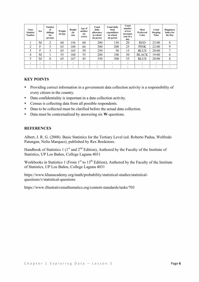
Once the data are contextualized, there is now meaning to the collection of number and symbols which may now look like the following which is just a small part of the data collected in the earlier activity.
C h a p t e r ( 1 ( E x p l o r i n g ( D a t a ( – ( L e s s o n ( 2 ( Page(6((
Class Student Number
Sex
Number of
siblings (in
person)
Weight (in kg)
Height (in cm)
Age of mother
(in years)
Usual daily
allowance in school (in pesos)
Usual daily food
expenditure in school (in pesos)
Usual number of text
messages sent in a
day
Most Preferred
Color
Usual Sleeping
Time
Happiness Index for the Day
1 M 2 60 156 60 200 150 20 RED 23:00 8 2 F 5 63 160 66 300 200 25 PINK 22:00 9 3 F 3 65 165 59 250 50 15 BLUE 20:00 7 4 M 1 55 160 55 200 100 30 BLACK 19:00 6 5 M 0 65 167 45 350 300 35 BLUE 20:00 8 : : : : : : : : : : : : : : : : : : : : : : : :
KEY POINTS
• Providing correct information in a government data collection activity is a responsibility of every citizen in the country.
• Data confidentiality is important in a data collection activity. • Census is collecting data from all possible respondents. • Data to be collected must be clarified before the actual data collection. • Data must be contextualized by answering six W-questions.
REFERENCES
Albert, J. R. G. (2008). Basic Statistics for the Tertiary Level (ed. Roberto Padua, Welfredo Patungan, Nelia Marquez), published by Rex Bookstore.
Handbook of Statistics 1 (1st and 2nd Edition), Authored by the Faculty of the Institute of Statistics, UP Los Baños, College Laguna 4031
Workbooks in Statistics 1 (From 1st to 13th Edition), Authored by the Faculty of the Institute of Statistics, UP Los Baños, College Laguna 4031
https://www.khanacademy.org/math/probability/statistical-studies/statistical-questions/v/statistical-questions
https://www.illustrativemathematics.org/content-standards/tasks/703
C h a p t e r ( 1 ( E x p l o r i n g ( D a t a ( – ( L e s s o n ( 2 ( Page(7((
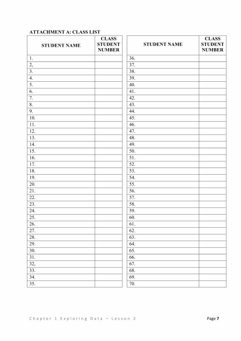
ATTACHMENT A: CLASS LIST
STUDENT NAME CLASS
STUDENT NUMBER
STUDENT NAME CLASS
STUDENT NUMBER
1. 36.
2, 37.
3. 38.
4. 39.
5. 40.
6. 41.(
7. 42.(
8. 43.(
9. 44.(
10. 45.(
11. 46.(
12. 47.(
13. 48.(
14. 49.(
15. 50.(
16. 51.(
17. 52.(
18. 53.(
19. 54.(
20. 55.(
21. 56.(
22. 57.(
23. 58.(
24. 59.(
25. 60.(
26. 61.(
27. 62.(
28. 63.(
29. 64.(
30. 65.(
31. 66.(
32, 67.(
33. 68.(
34. 69.(
35. 70.(
C h a p t e r ( 1 ( E x p l o r i n g ( D a t a ( – ( L e s s o n ( 2 ( Page(8((
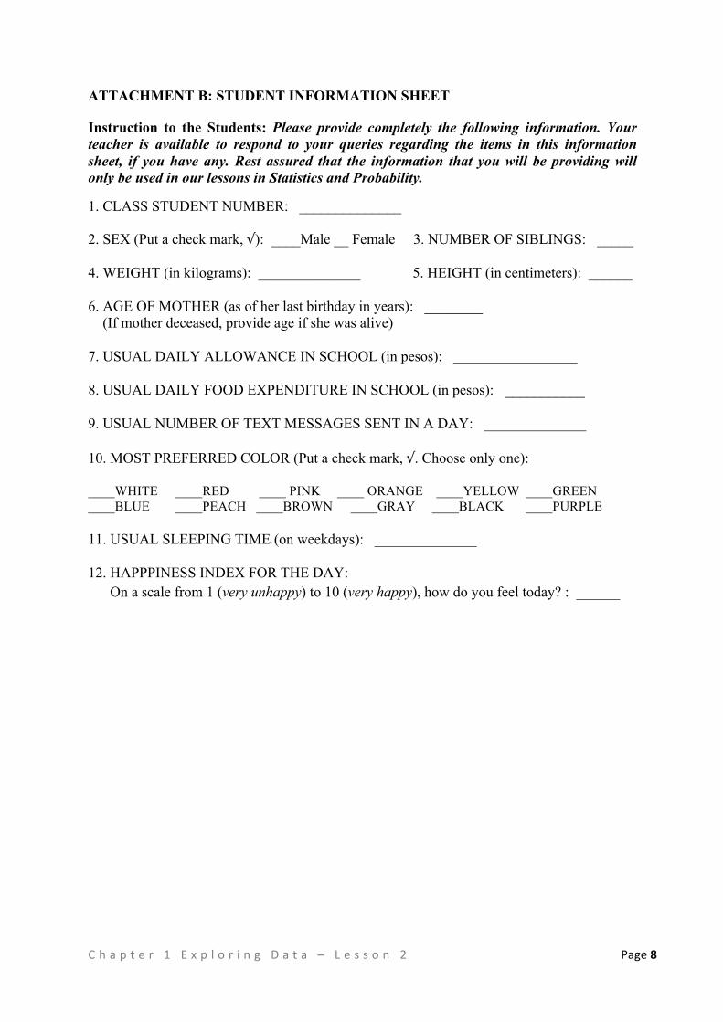
ATTACHMENT B: STUDENT INFORMATION SHEET
Instruction to the Students: Please provide completely the following information. Your teacher is available to respond to your queries regarding the items in this information sheet, if you have any. Rest assured that the information that you will be providing will only be used in our lessons in Statistics and Probability.
1. CLASS STUDENT NUMBER: ______________
2. SEX (Put a check mark, √): ____Male __ Female 3. NUMBER OF SIBLINGS: _____ 4. WEIGHT (in kilograms): ______________ 5. HEIGHT (in centimeters): ______ 6. AGE OF MOTHER (as of her last birthday in years): ________ (If mother deceased, provide age if she was alive) 7. USUAL DAILY ALLOWANCE IN SCHOOL (in pesos): _________________ 8. USUAL DAILY FOOD EXPENDITURE IN SCHOOL (in pesos): ___________ 9. USUAL NUMBER OF TEXT MESSAGES SENT IN A DAY: ______________ 10. MOST PREFERRED COLOR (Put a check mark, √. Choose only one): ____WHITE ____RED ____ PINK ____ ORANGE ____YELLOW ____GREEN ____BLUE ____PEACH ____BROWN ____GRAY ____BLACK ____PURPLE 11. USUAL SLEEPING TIME (on weekdays): ______________ 12. HAPPPINESS INDEX FOR THE DAY:
On a scale from 1 (very unhappy) to 10 (very happy), how do you feel today? : ______
C h a p t e r ( 1 ( E x p l o r i n g ( D a t a ( – ( L e s s o n ( 2 ( Page(9((
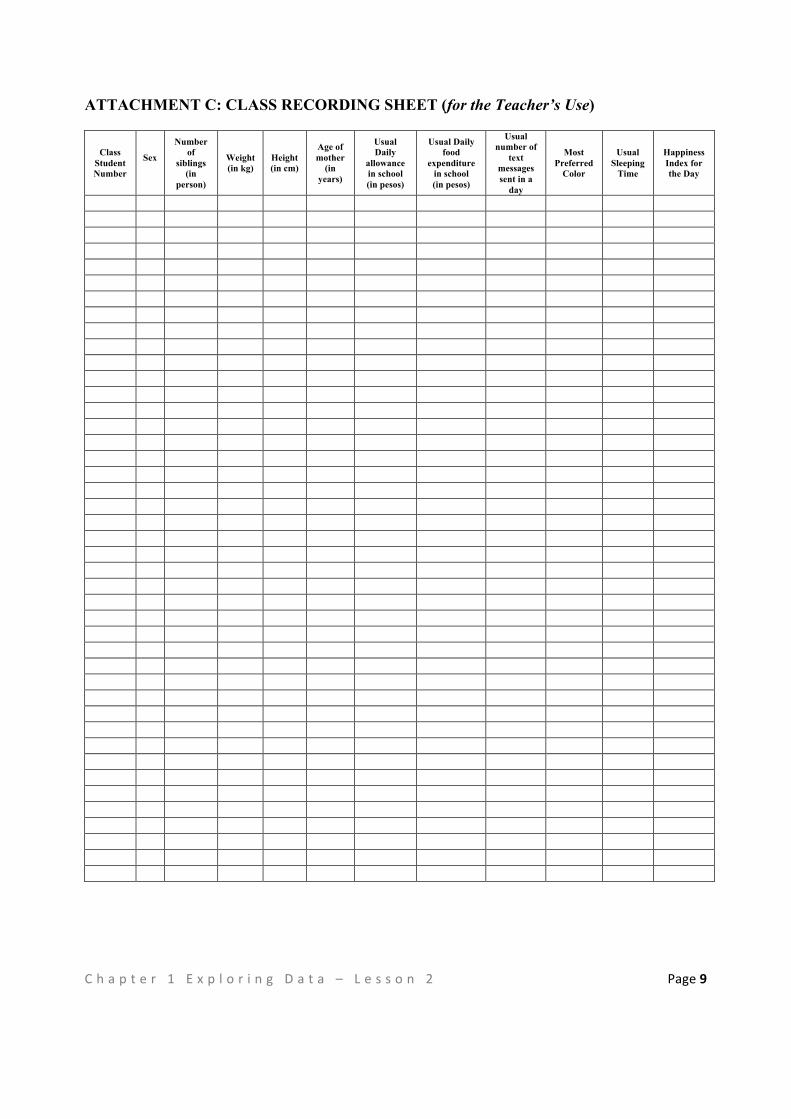
ATTACHMENT C: CLASS RECORDING SHEET (for the Teacher’s Use)
Class Student Number
Sex
Number of
siblings (in
person)
Weight (in kg)
Height (in cm)
Age of mother
(in years)
Usual Daily
allowance in school (in pesos)
Usual Daily food
expenditure in school (in pesos)
Usual number of
text messages sent in a
day
Most Preferred
Color
Usual Sleeping
Time
Happiness Index for the Day
!C h a p t e r ! 1 ! E x p l o r i n g ! D a t a ! – ! L e s s o n ! 3 ! Page!1"! !!!!
Chapter 1:Exploring Data Lesson 3: Basic Terms in Statistics
TIME FRAME:1 hour session OVERVIEW OF LESSON
As continuation of Lesson 2 (where we contextualize data) in this lesson we define basic terms in statistics as we continue to explore data. These basic terms include the universe, variable, population and sample. In detail we will discuss other concepts in relation to a variable.
LEARNING OUTCOME(S): At the end of the lesson, the learner is able to • Define universe and differentiate it with population; and • Define and differentiate between qualitative and quantitative variables, and between
discrete and continuous variables (that are quantitative);
LESSON OUTLINE:
1. Recall previous lesson on ‘Contextualizing Data’ 2. Definition of Basic Terms in Statistics (universe, variable, population and sample) 3. Broad of Classification of Variables(qualitative and quantitative, discrete and continuous)
DEVELOPMENT OF THE LESSON
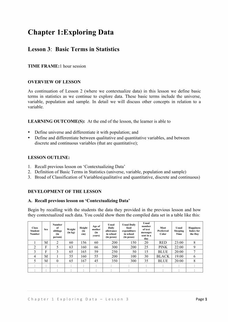
A. Recall previous lesson on ‘Contextualizing Data’
Begin by recalling with the students the data they provided in the previous lesson and how they contextualized such data. You could show them the compiled data set in a table like this:
Class Student Number
Sex
Number of
siblings (in
person)
Weight (in kg)
Height (in cm)
Age of mother
(in years)
Usual Daily
allowance in school (in pesos)
Usual Daily food
expenditure in school (in pesos)
Usual number of text
messages sent in a
day
Most Preferred
Color
Usual Sleeping
Time
Happiness Index for the Day
1 M 2 60 156 60 200 150 20 RED 23:00 8 2 F 5 63 160 66 300 200 25 PINK 22:00 9 3 F 3 65 165 59 250 50 15 BLUE 20:00 7 4 M 1 55 160 55 200 100 30 BLACK 19:00 6 5 M 0 65 167 45 350 300 35 BLUE 20:00 8 : : : : : : : : : : : : : : : : : : : : : : : :
!C h a p t e r ! 1 ! E x p l o r i n g ! D a t a ! – ! L e s s o n ! 3 ! Page!2"! !!!!
Recall also their response on the first Ws of the data, that is, on the question “Who provided the data?” We said last time the students of the class provided the data or the data were taken from the students.
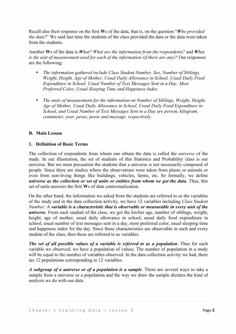
Another Ws of the data is What? What are the information from the respondents? and What is the unit of measurement used for each of the information (if there are any)? Our responses are the following:
• The information gathered include Class Student Number, Sex, Number of Siblings, Weight, Height, Age of Mother, Usual Daily Allowance in School, Usual Daily Food Expenditure in School, Usual Number of Text Messages Sent in a Day, Most Preferred Color, Usual Sleeping Time and Happiness Index.
• The units of measurement for the information on Number of Siblings, Weight, Height, Age of Mother, Usual Daily Allowance in School, Usual Daily Food Expenditure in School, and Usual Number of Text Messages Sent in a Day are person, kilogram, centimeter, year, pesos, pesos and message, respectively.
B. Main Lesson
1. Definition of Basic Terms
The collection of respondents from whom one obtain the data is called the universe of the study. In our illustration, the set of students of this Statistics and Probability class is our universe. But we must precaution the students that a universe is not necessarily composed of people. Since there are studies where the observations were taken from plants or animals or even from non-living things like buildings, vehicles, farms, etc. So formally, we define universe as the collection or set of units or entities from whom we got the data. Thus, this set of units answers the first Ws of data contextualization.
On the other hand, the information we asked from the students are referred to as the variables of the study and in the data collection activity, we have 12 variables including Class Student Number. A variable is a characteristic that is observable or measurable in every unit of the universe. From each student of the class, we got the his/her age, number of siblings, weight, height, age of mother, usual daily allowance in school, usual daily food expenditure in school, usual number of text messages sent in a day, most preferred color, usual sleeping time and happiness index for the day. Since these characteristics are observable in each and every student of the class, then these are referred to as variables.
The set of all possible values of a variable is referred to as a population. Thus for each variable we observed, we have a population of values. The number of population in a study will be equal to the number of variables observed. In the data collection activity we had, there are 12 populations corresponding to 12 variables.
A subgroup of a universe or of a population is a sample. There are several ways to take a sample from a universe or a population and the way we draw the sample dictates the kind of analysis we do with our data.
!C h a p t e r ! 1 ! E x p l o r i n g ! D a t a ! – ! L e s s o n ! 3 ! Page!3"! !!!!
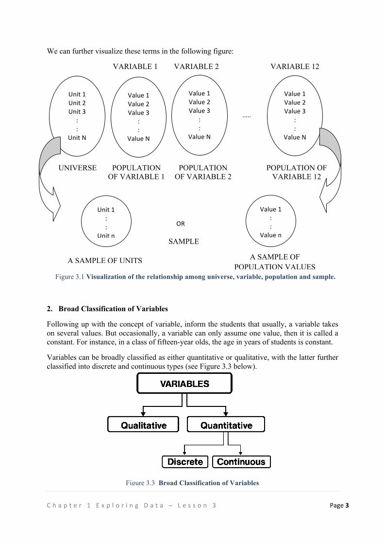
We can further visualize these terms in the following figure:
VARIABLE 1 VARIABLE 2 VARIABLE 12
UNIVERSE POPULATION OF VARIABLE 1
POPULATION OF VARIABLE 2
POPULATION OF VARIABLE 12
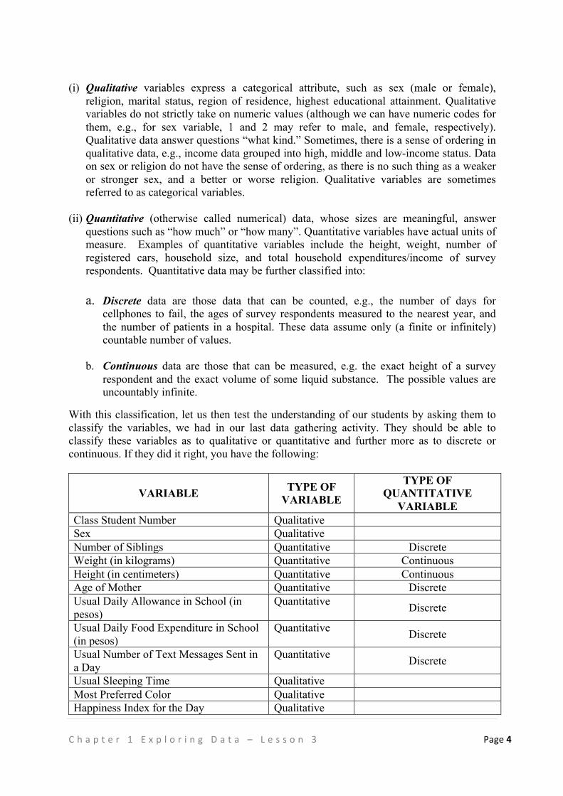
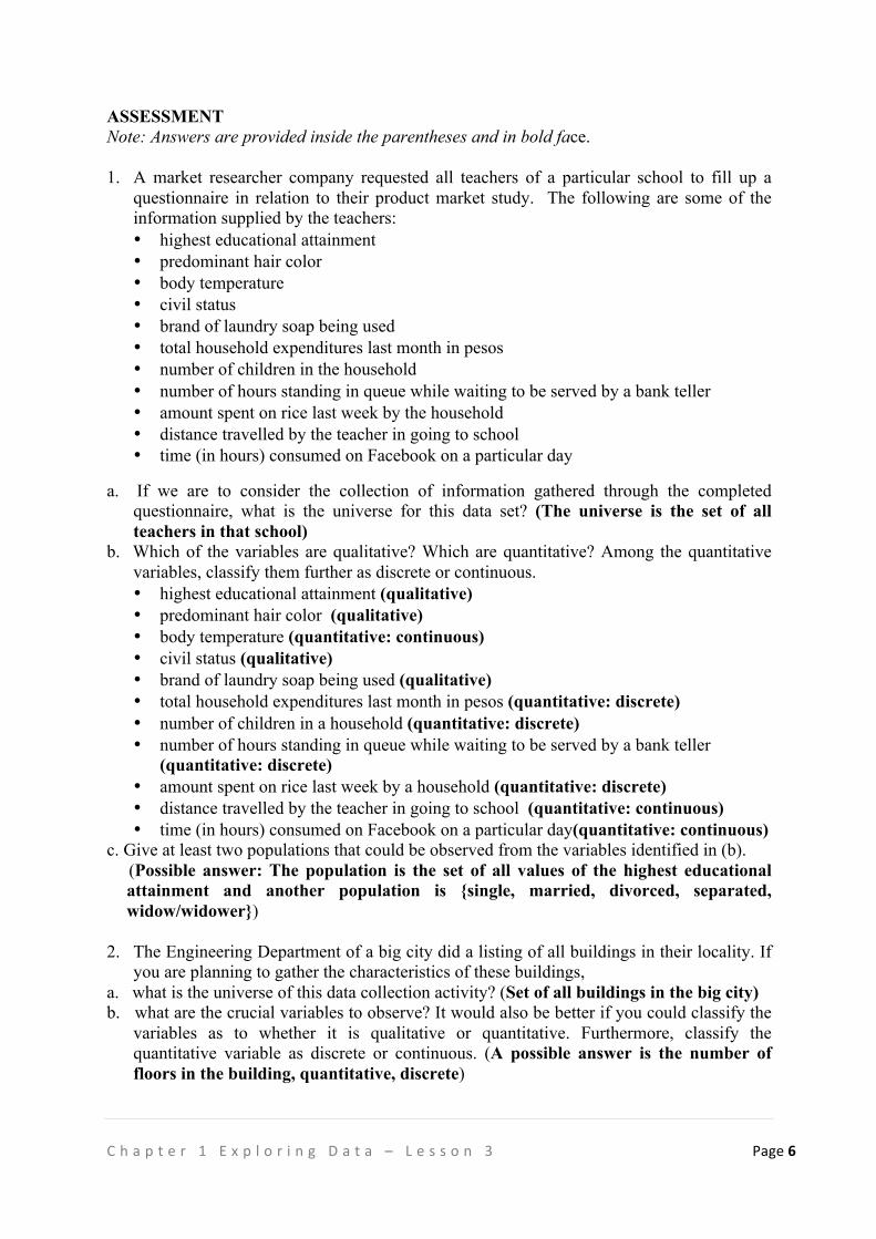
2. Broad Classification of Variables
Following up with the concept of variable, inform the students that usually, a variable takes on several values. But occasionally, a variable can only assume one value, then it is called a constant. For instance, in a class of fifteen-year olds, the age in years of students is constant.
Variables can be broadly classified as either quantitative or qualitative, with the latter further classified into discrete and continuous types (see Figure 3.3 below).
Unit!1!Unit!2!Unit!3!
:!:!
Unit!N!
Value!1!Value!2!Value!3!
:!:!
Value!N!
Value!1!Value!2!Value!3!
:!:!
Value!N!!
Value!1!Value!2!Value!3!
:!:!
Value!N!!
…..!
OR!
Unit!1!:!:!
Unit!n!
Value!1!:!:!
Value!n!SAMPLE
Figure 3.3 Broad Classification of Variables
A SAMPLE OF UNITS A SAMPLE OF POPULATION VALUES
Figure 3.1 Visualization of the relationship among universe, variable, population and sample.
!C h a p t e r ! 1 ! E x p l o r i n g ! D a t a ! – ! L e s s o n ! 3 ! Page!4"! !!!!
(i) Qualitative variables express a categorical attribute, such as sex (male or female),
religion, marital status, region of residence, highest educational attainment. Qualitative variables do not strictly take on numeric values (although we can have numeric codes for them, e.g., for sex variable, 1 and 2 may refer to male, and female, respectively). Qualitative data answer questions “what kind.” Sometimes, there is a sense of ordering in qualitative data, e.g., income data grouped into high, middle and low-income status. Data on sex or religion do not have the sense of ordering, as there is no such thing as a weaker or stronger sex, and a better or worse religion. Qualitative variables are sometimes referred to as categorical variables.
(ii) Quantitative (otherwise called numerical) data, whose sizes are meaningful, answer questions such as “how much” or “how many”. Quantitative variables have actual units of measure. Examples of quantitative variables include the height, weight, number of registered cars, household size, and total household expenditures/income of survey respondents. Quantitative data may be further classified into:
a. Discrete data are those data that can be counted, e.g., the number of days for
cellphones to fail, the ages of survey respondents measured to the nearest year, and the number of patients in a hospital. These data assume only (a finite or infinitely) countable number of values.
b. Continuous data are those that can be measured, e.g. the exact height of a survey
respondent and the exact volume of some liquid substance. The possible values are uncountably infinite.
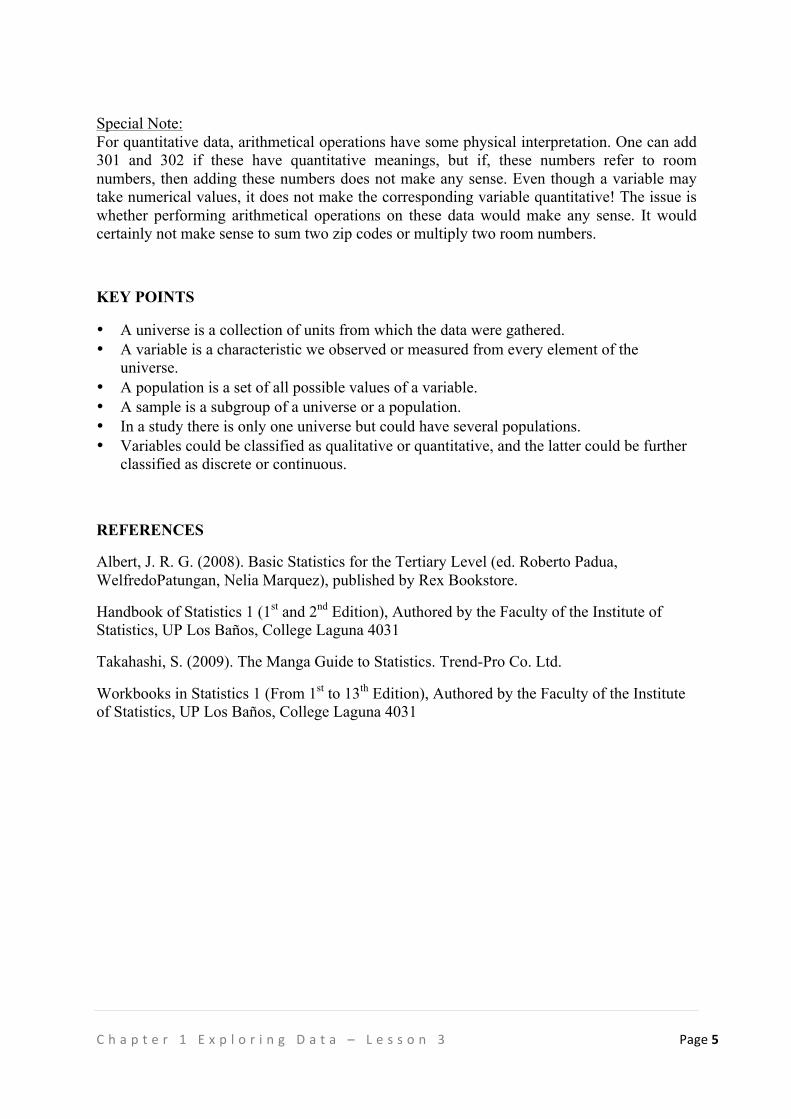
With this classification, let us then test the understanding of our students by asking them to classify the variables, we had in our last data gathering activity. They should be able to classify these variables as to qualitative or quantitative and further more as to discrete or continuous. If they did it right, you have the following:
VARIABLE TYPE OF VARIABLE
TYPE OF QUANTITATIVE
VARIABLE Class Student Number Qualitative Sex Qualitative Number of Siblings Quantitative Discrete Weight (in kilograms) Quantitative Continuous Height (in centimeters) Quantitative Continuous Age of Mother Quantitative Discrete Usual Daily Allowance in School (in pesos)
Quantitative Discrete
Usual Daily Food Expenditure in School (in pesos)
Quantitative Discrete
Usual Number of Text Messages Sent in a Day
Quantitative Discrete
Usual Sleeping Time Qualitative Most Preferred Color Qualitative Happiness Index for the Day Qualitative
!C h a p t e r ! 1 ! E x p l o r i n g ! D a t a ! – ! L e s s o n ! 3 ! Page!5"! !!!!
Special Note: For quantitative data, arithmetical operations have some physical interpretation. One can add 301 and 302 if these have quantitative meanings, but if, these numbers refer to room numbers, then adding these numbers does not make any sense. Even though a variable may take numerical values, it does not make the corresponding variable quantitative! The issue is whether performing arithmetical operations on these data would make any sense. It would certainly not make sense to sum two zip codes or multiply two room numbers.
KEY POINTS
• A universe is a collection of units from which the data were gathered. • A variable is a characteristic we observed or measured from every element of the
universe. • A population is a set of all possible values of a variable. • A sample is a subgroup of a universe or a population. • In a study there is only one universe but could have several populations. • Variables could be classified as qualitative or quantitative, and the latter could be further
classified as discrete or continuous.
REFERENCES
Albert, J. R. G. (2008). Basic Statistics for the Tertiary Level (ed. Roberto Padua, WelfredoPatungan, Nelia Marquez), published by Rex Bookstore.
Handbook of Statistics 1 (1st and 2nd Edition), Authored by the Faculty of the Institute of Statistics, UP Los Baños, College Laguna 4031
Takahashi, S. (2009). The Manga Guide to Statistics. Trend-Pro Co. Ltd.
Workbooks in Statistics 1 (From 1st to 13th Edition), Authored by the Faculty of the Institute of Statistics, UP Los Baños, College Laguna 4031
!C h a p t e r ! 1 ! E x p l o r i n g ! D a t a ! – ! L e s s o n ! 3 ! Page!6"! !!!!
ASSESSMENT Note: Answers are provided inside the parentheses and in bold face. 1. A market researcher company requested all teachers of a particular school to fill up a
questionnaire in relation to their product market study. The following are some of the information supplied by the teachers: • highest educational attainment • predominant hair color • body temperature • civil status • brand of laundry soap being used • total household expenditures last month in pesos • number of children in the household • number of hours standing in queue while waiting to be served by a bank teller • amount spent on rice last week by the household • distance travelled by the teacher in going to school • time (in hours) consumed on Facebook on a particular day
a. If we are to consider the collection of information gathered through the completed questionnaire, what is the universe for this data set? (The universe is the set of all teachers in that school)
b. Which of the variables are qualitative? Which are quantitative? Among the quantitative variables, classify them further as discrete or continuous. • highest educational attainment (qualitative) • predominant hair color (qualitative) • body temperature (quantitative: continuous) • civil status (qualitative) • brand of laundry soap being used (qualitative) • total household expenditures last month in pesos (quantitative: discrete) • number of children in a household (quantitative: discrete) • number of hours standing in queue while waiting to be served by a bank teller
(quantitative: discrete) • amount spent on rice last week by a household (quantitative: discrete) • distance travelled by the teacher in going to school (quantitative: continuous) • time (in hours) consumed on Facebook on a particular day(quantitative: continuous)
c. Give at least two populations that could be observed from the variables identified in (b). (Possible answer: The population is the set of all values of the highest educational
attainment and another population is {single, married, divorced, separated, widow/widower})
2. The Engineering Department of a big city did a listing of all buildings in their locality. If
you are planning to gather the characteristics of these buildings, a. what is the universe of this data collection activity? (Set of all buildings in the big city) b. what are the crucial variables to observe? It would also be better if you could classify the
variables as to whether it is qualitative or quantitative. Furthermore, classify the quantitative variable as discrete or continuous. (A possible answer is the number of floors in the building, quantitative, discrete)
!C h a p t e r ! 1 ! E x p l o r i n g ! D a t a ! – ! L e s s o n ! 3 ! Page!7"! !!!!
3. A survey of students in a certain school is conducted. The survey questionnaire details the information on the following variables. For each of these variables, identify whether the variable is qualitative or quantitative, and if the latter, state whether it is discrete or continuous. a. number of family members who are working (quantitative: discrete) b. ownership of a cell phone among family members (qualitative) c. length (in minutes) of longest call made on each cell phone owned per month
(quantitative: continuous) d. ownership/rental of dwelling (qualitative) e. amount spent in pesos on food in one week (quantitative: discrete) f. occupation of household head (qualitative) g. total family income (quantitative: discrete) h. number of years of schooling of each family member (quantitative: discrete) i. access of family members to social media (qualitative) j. amount of time last week spent by each family member using the internet
(quantitative: continuous)
Explanatory Note:
• Teachers have the option to just ask this assessment orally to the entire class, or to group students and ask them to identify answers, or to give this as homework, or to use some questions/items here for a chapter examination.
!C h a p t e r ! 1 ! E x p l o r i n g ! D a t a ! – ! L e s s o n ! 4 ! Page!1"! !!!!
Chapter 1: Exploring Data Lesson 4: Levels of Measurement
TIME FRAME:1 hour session OVERVIEW OF LESSON
In this lesson we discuss the different levels of measurement as we continue to explore data. Knowing such will enable us to plan the data collection process we need to employ in order to gather the appropriate data for analysis.
LEARNING OUTCOME(S): At the end of the lesson, the learner is able to identify and differentiate the different levels of measurement and methods of data collection LESSON OUTLINE:
1. Motivational Activity 2. Levels of Measurement 3. Data Collection Methods
DEVELOPMENT OF THE LESSON
A. Motivational Activity
Ask the students first if they believe the following statement: “Students who eat a healthy breakfast will do best on a quiz, students who eat an unhealthy breakfast will get an average performance, and students who do not eat anything for breakfast will do the worst on a quiz” You could further ask one or more students who have different answers to defend their answers. Then challenge the students to apply a statistical process to investigate on the validity of this statement. You could enumerate on the board the steps in the process to undertake like the following: 1. Plan or design the collection of data to verify the validity of the statement in a way that
maximizes information content and minimizes bias; 2. Collect the data as required in the plan; 3. Verify the quality of the data after it was collected; 4. Summarize the information extracted from the data; and 5. Examine the summary statistics so that insight and meaningful information can be
produced to support your decision whether to believe or not the given statement.
!C h a p t e r ! 1 ! E x p l o r i n g ! D a t a ! – ! L e s s o n ! 4 ! Page!2"! !!!!
Let us discuss in detail the first step. In planning or designing the data collection activity, we could consider the set of all the students in the class as our universe. Then let us identify the variables we need to observe or measure to verify the validity of the statement. You may ask the students to participate in the discussion by asking them to identify a question to get the needed data. The following are some possible suggested queries: 1. Do you usually have a breakfast before going to school?
(Note: This is answerable by Yes or No) 2. What do you usually have for breakfast?
(Note: Possible responses for this question are rice, bread, banana, oatmeal, cereal, etc)
The responses in Questions Numbers 1 and 2 could lead us to identify whether a student in the class had a healthy breakfast, an unhealthy breakfast or no breakfast at all.
Furthermore, there is a need to determine the performance of the student in a quiz on that day. The score in the quiz could be used to identify the student’s performance as best, average or worst.
As we describe the data collection process to verify the validity of the statement, there is also a need to include the levels of measurement for the variables of interest.
B. Main Lesson:
1. Levels of Measurement
Inform students that there are four levels of measurement of variables: nominal, ordinal, interval and ratio. These are hierarchical in nature and are described as follows:
Nominal level of measurement arises when we have variables that are categorical and non-numeric or where the numbers have no sense of ordering. As an example, consider the numbers on the uniforms of basketball players. Is the player wearing a number 7 a worse player than the player wearing number 10? Maybe, or maybe not, but the number on the uniform does not have anything to do with their performance. The numbers on the uniform merely help identify the basketball player. Other examples of the variables measured at the nominal level include sex, marital status, religious affiliation. For the study on the validity of the statement regarding effect of breakfast on school performance, students who responded Yes to Question Number 1 can be coded 1 while those who responded No, code 0 can be assigned. The numbers used are simply for numerical codes, and cannot be used for ordering and any mathematical computation. Ordinal level also deals with categorical variables like the nominal level, but in this level ordering is important, that is the values of the variable could be ranked. For the study on the validity of the statement regarding effect of breakfast on school performance, students who had healthy breakfast can be coded 1, those who had unhealthy breakfast as 2 while those who had no breakfast at all as 3. Using the codes the responses could be ranked. Thus, the students who had a healthy breakfast are ranked first while those who had no breakfast at all are ranked last in terms of having a healthy breakfast. The numerical codes here have a meaningful sense of ordering, unlike basketball player uniforms, the numerical codes suggest that one student is having a healthier breakfast than another student. Other examples of the ordinal scale include socio economic status (A to E, where A is wealthy, E is poor), difficulty
!C h a p t e r ! 1 ! E x p l o r i n g ! D a t a ! – ! L e s s o n ! 4 ! Page!3"! !!!!
of questions in an exam (easy, medium difficult), rank in a contest (first place, second place, etc.), and perceptions in Likert scales. Note to Teacher: Let us also emphasize to the students that while there is a sense or ordering, there is no zero point in an ordinal scale. In addition, there is no way to find out how much “distance” there is between one category and another. In a scale from 1 to 10, the difference between 7 and 8 may not be the same difference between 1 and 2. Interval level tells us that one unit differs by a certain amount of degree from another unit. Knowing how much one unit differs from another is an additional property of the interval level on top of having the properties posses by the ordinal level. When measuring temperature in Celsius, a 10 degree difference has the same meaning anywhere along the scale – the difference between 10 and 20 degree Celsius is the same as between 80 and 90 centigrade. But, we cannot say that 80 degrees Celsius is twice as hot as 40 degrees Celsius since there is no true zero, but only an arbitrary zero point. A measurement of 0 degrees Celsius does not reflect a true "lack of temperature." Thus, Celsius scale is in interval level. Other example of a variable measure at the interval is the Intelligence Quotient (IQ) of a person. We can tell not only which person ranks higher in IQ but also how much higher he or she ranks with another, but zero IQ does not mean no intelligence. The students could also be classified or categorized according to their IQ level. Hence, the IQ as measured in the interval level has also the properties of those measured in the ordinal as well as those in the nominal level.
Special Note: Inform also the students that the interval level allows addition and subtraction operations, but it does not possess an absolute zero. Zero is arbitrary as it does not mean the value does not exist. Zero only represents an additional measurement point.
Ratio level also tells us that one unit has so many times as much of the property as does another unit. The ratio level possesses a meaningful (unique and non-arbitrary) absolute, fixed zero point and allows all arithmetic operations. The existence of the zero point is the only difference between ratio and interval level of measurement. Examples of the ratio scale include mass, heights, weights, energy and electric charge. With mass as an example, the difference between 120 grams and 135 grams is 15 grams, and this is the same difference between 380 grams and 395 grams. The level at any given point is constant, and a measurement of 0 reflects a complete lack of mass. Amount of money is also at the ratio level. We can say that 2000 pesos is twice more than 1,000 pesos. In addition, money has a true zero point: if you have zero money, this implies the absence of money. For the study on the validity of the statement regarding effect of breakfast on school performance, the student’s score in the quiz is measured at the ratio level. A score of zero implies that the student did not get a correct answer at all.
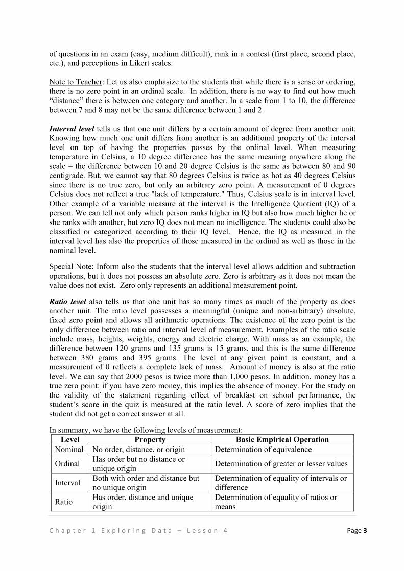
In summary, we have the following levels of measurement: Level Property Basic Empirical Operation
Nominal No order, distance, or origin Determination of equivalence
Ordinal Has order but no distance or unique origin Determination of greater or lesser values
Interval Both with order and distance but no unique origin
Determination of equality of intervals or difference
Ratio Has order, distance and unique origin
Determination of equality of ratios or means
!C h a p t e r ! 1 ! E x p l o r i n g ! D a t a ! – ! L e s s o n ! 4 ! Page!4"! !!!!
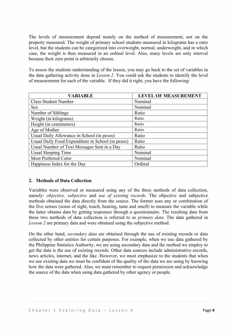
The levels of measurement depend mainly on the method of measurement, not on the property measured. The weight of primary school students measured in kilograms has a ratio level, but the students can be categorized into overweight, normal, underweight, and in which case, the weight is then measured in an ordinal level. Also, many levels are only interval because their zero point is arbitrarily chosen. To assess the students understanding of the lesson, you may go back to the set of variables in the data gathering activity done in Lesson 2. You could ask the students to identify the level of measurement for each of the variable. If they did it right, you have the following:
VARIABLE LEVEL OF MEASUREMENT
Class Student Number Nominal Sex Nominal Number of Siblings Ratio Weight (in kilograms) Ratio Height (in centimeters) Ratio Age of Mother Ratio Usual Daily Allowance in School (in pesos) Ratio Usual Daily Food Expenditure in School (in pesos) Ratio Usual Number of Text Messages Sent in a Day Ratio Usual Sleeping Time Nominal Most Preferred Color Nominal Happiness Index for the Day Ordinal
2. Methods of Data Collection
Variables were observed or measured using any of the three methods of data collection, namely: objective, subjective and use of existing records. The objective and subjective methods obtained the data directly from the source. The former uses any or combination of the five senses (sense of sight, touch, hearing, taste and smell) to measure the variable while the latter obtains data by getting responses through a questionnaire. The resulting data from these two methods of data collection is referred to as primary data. The data gathered in Lesson 2 are primary data and were obtained using the subjective method. On the other hand, secondary data are obtained through the use of existing records or data collected by other entities for certain purposes. For example, when we use data gathered by the Philippine Statistics Authority, we are using secondary data and the method we employ to get the data is the use of existing records. Other data sources include administrative records, news articles, internet, and the like. However, we must emphasize to the students that when we use existing data we must be confident of the quality of the data we are using by knowing how the data were gathered. Also, we must remember to request permission and acknowledge the source of the data when using data gathered by other agency or people.
!C h a p t e r ! 1 ! E x p l o r i n g ! D a t a ! – ! L e s s o n ! 4 ! Page!5"! !!!!
KEY POINTS
• Four levels of measurement: Nominal, Ordinal, Interval and Ratio • Knowing what level the variable was measured or observed will guide us to know the
type of analysis to apply. • Three methods of data collection include objective, subjective and use of existing records. • Using the data collection method as basis, data can be classified as either primary or
secondary data.
REFERENCES
Albert, J. R. G. (2008). Basic Statistics for the Tertiary Level (ed. Roberto Padua, Welfredo Patungan, Nelia Marquez), published by Rex Bookstore.
Handbook of Statistics 1 (1st and 2nd Edition), Authored by the Faculty of the Institute of Statistics, UP Los Baños, College Laguna 4031
Takahashi, S. (2009). The Manga Guide to Statistics. Trend-Pro Co. Ltd.
Workbooks in Statistics 1 (From 1st to 13th Edition), Authored by the Faculty of the Institute of Statistics, UP Los Baños, College Laguna 4031
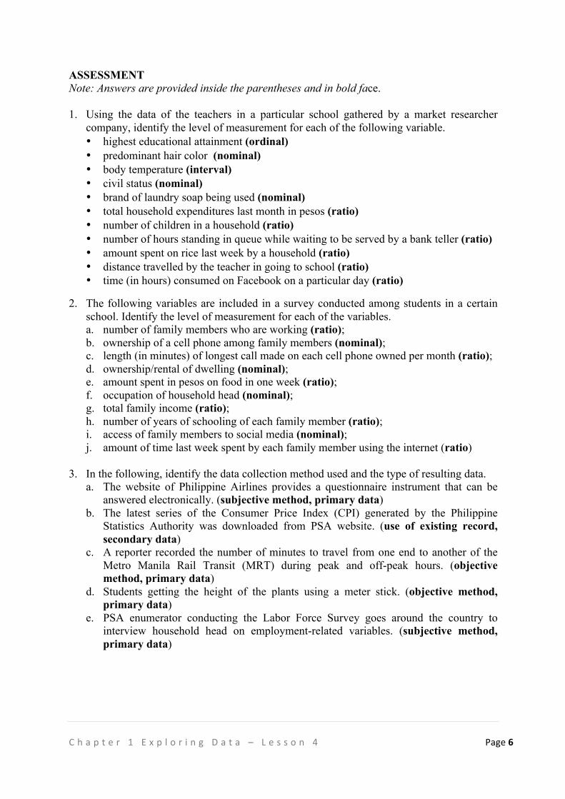
!C h a p t e r ! 1 ! E x p l o r i n g ! D a t a ! – ! L e s s o n ! 4 ! Page!6"! !!!!
ASSESSMENT Note: Answers are provided inside the parentheses and in bold face. 1. Using the data of the teachers in a particular school gathered by a market researcher
company, identify the level of measurement for each of the following variable. • highest educational attainment (ordinal) • predominant hair color (nominal) • body temperature (interval) • civil status (nominal) • brand of laundry soap being used (nominal) • total household expenditures last month in pesos (ratio) • number of children in a household (ratio) • number of hours standing in queue while waiting to be served by a bank teller (ratio) • amount spent on rice last week by a household (ratio) • distance travelled by the teacher in going to school (ratio) • time (in hours) consumed on Facebook on a particular day (ratio)
2. The following variables are included in a survey conducted among students in a certain school. Identify the level of measurement for each of the variables. a. number of family members who are working (ratio); b. ownership of a cell phone among family members (nominal); c. length (in minutes) of longest call made on each cell phone owned per month (ratio); d. ownership/rental of dwelling (nominal); e. amount spent in pesos on food in one week (ratio); f. occupation of household head (nominal); g. total family income (ratio); h. number of years of schooling of each family member (ratio); i. access of family members to social media (nominal); j. amount of time last week spent by each family member using the internet (ratio)
3. In the following, identify the data collection method used and the type of resulting data. a. The website of Philippine Airlines provides a questionnaire instrument that can be
answered electronically. (subjective method, primary data) b. The latest series of the Consumer Price Index (CPI) generated by the Philippine
Statistics Authority was downloaded from PSA website. (use of existing record, secondary data)
c. A reporter recorded the number of minutes to travel from one end to another of the Metro Manila Rail Transit (MRT) during peak and off-peak hours. (objective method, primary data)
d. Students getting the height of the plants using a meter stick. (objective method, primary data)
e. PSA enumerator conducting the Labor Force Survey goes around the country to interview household head on employment-related variables. (subjective method, primary data)
!C h a p t e r ! 1 ! E x p l o r i n g ! D a t a ! – ! L e s s o n ! 5 ! Page!1"! !!!!
Chapter 1: Exploring Data Lesson 5: Data Presentation
TIME FRAME:1 hour session OVERVIEW OF LESSON
In this lesson we enrich what the students have already learned from Grade 1 to 10 about presenting data. Additional concepts could help the students to appropriately describe further the data set.
LEARNING OUTCOME(S): At the end of the lesson, the learner is able to identify and use the appropriate method of presenting information from a data set effectively. LESSON OUTLINE:
1. Review of Lessons in Data Presentation taken up from Grade 1 to 10. 2. Methods of Data Presentation 3. The Frequency Distribution Table and Histogram
DEVELOPMENT OF THE LESSON
A. Review of Lessons in Data Presentation taken up from Grade 1 to 10.
You could assist the students to recall what they have learned in Grade 1 to 10 regarding data presentation by asking them to participate in an activity. The activity is called ‘Toss the Ball’. This is actually a review and wake-up exercise. Toss a ball to a student and he/she will give the most important concept he/she learned about data presentation. You may list on the board their responses. You could summarize their responses to be able to establish what they already know about data presentation techniques and from this you could build other concepts on the topic. A suggestion is to classify their answers according to the three methods of data presentation, i.e. textual, tabular and graphical. A possible listing will be something like this:
Textual or Narrative Presentation: • Detailed information are given in textual presentation • Narrative report is a way to present data.
Tabular Presentation: • Numerical values are presented using tables. • Information are lost in tabular presentation of data. • Frequency distribution table is also applicable for qualitative variables
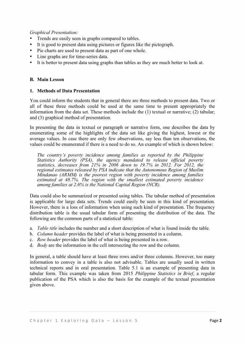
!C h a p t e r ! 1 ! E x p l o r i n g ! D a t a ! – ! L e s s o n ! 5 ! Page!2"! !!!!
Graphical Presentation: • Trends are easily seen in graphs compared to tables. • It is good to present data using pictures or figures like the pictograph. • Pie charts are used to present data as part of one whole. • Line graphs are for time-series data. • It is better to present data using graphs than tables as they are much better to look at. B. Main Lesson
1. Methods of Data Presentation
You could inform the students that in general there are three methods to present data. Two or all of these three methods could be used at the same time to present appropriately the information from the data set. These methods include the (1) textual or narrative; (2) tabular; and (3) graphical method of presentation.
In presenting the data in textual or paragraph or narrative form, one describes the data by enumerating some of the highlights of the data set like giving the highest, lowest or the average values. In case there are only few observations, say less than ten observations, the values could be enumerated if there is a need to do so. An example of which is shown below:
The country’s poverty incidence among families as reported by the Philippine Statistics Authority (PSA), the agency mandated to release official poverty statistics, decreases from 21% in 2006 down to 19.7% in 2012. For 2012, the regional estimates released by PSA indicate that the Autonomous Region of Muslim Mindanao (ARMM) is the poorest region with poverty incidence among families estimated at 48.7%. The region with the smallest estimated poverty incidence among families at 2.6% is the National Capital Region (NCR).
Data could also be summarized or presented using tables. The tabular method of presentation is applicable for large data sets. Trends could easily be seen in this kind of presentation. However, there is a loss of information when using such kind of presentation. The frequency distribution table is the usual tabular form of presenting the distribution of the data. The following are the common parts of a statistical table:
a. Table title includes the number and a short description of what is found inside the table. b. Column header provides the label of what is being presented in a column. c. Row header provides the label of what is being presented in a row. d. Body are the information in the cell intersecting the row and the column. In general, a table should have at least three rows and/or three columns. However, too many information to convey in a table is also not advisable. Tables are usually used in written technical reports and in oral presentation. Table 5.1 is an example of presenting data in tabular form. This example was taken from 2015 Philippine Statistics in Brief, a regular publication of the PSA which is also the basis for the example of the textual presentation given above.
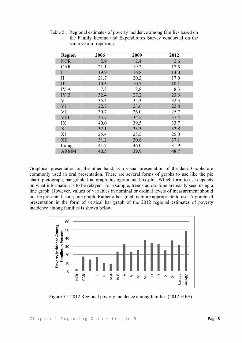
!C h a p t e r ! 1 ! E x p l o r i n g ! D a t a ! – ! L e s s o n ! 5 ! Page!3"! !!!!
Table 5.1 Regional estimates of poverty incidence among families based on the Family Income and Expenditures Survey conducted on the same year of reporting.
Region 2006 2009 2012 NCR 2.9 2.4 2.6 CAR 21.1 19.2 17.5 I 19.9 16.8 14.0 II 21.7 20.2 17.0 III 10.3 10.7 10.1 IV A 7.8 8.8 8.3 IV B 32.4 27.2 23.6 V 35.4 35.3 32.3 VI 22.7 23.6 22.8 VII 30.7 26.0 25.7 VIII 33.7 34.5 37.4 IX 40.0 39.5 33.7 X 32.1 33.3 32.8 XI 25.4 25.5 25.0 XII 31.2 30.8 37.1 Caraga 41.7 46.0 31.9 ARMM 40.5 39.9 48.7
Graphical presentation on the other hand, is a visual presentation of the data. Graphs are commonly used in oral presentation. There are several forms of graphs to use like the pie chart, pictograph, bar graph, line graph, histogram and box-plot. Which form to use depends on what information is to be relayed. For example, trends across time are easily seen using a line graph. However, values of variables in nominal or ordinal levels of measurement should not be presented using line graph. Rather a bar graph is more appropriate to use. A graphical presentation in the form of vertical bar graph of the 2012 regional estimates of poverty incidence among families is shown below:
Figure 5.1 2012 Regional poverty incidence among families (2012 FIES).
0!
10!
20!
30!
40!
50!
60!
NCR
!
CAR! I! II! III!
IV!A!
IV!B! V! VI!
VII!
VIII! IX! X! XI!
XII!
Caraga!
ARMM!
Poverty"Incide
nce"Am
ong"
Families"in"Percent"
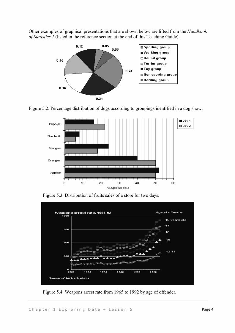
!C h a p t e r ! 1 ! E x p l o r i n g ! D a t a ! – ! L e s s o n ! 5 ! Page!4"! !!!!
Other examples of graphical presentations that are shown below are lifted from the Handbook of Statistics 1 (listed in the reference section at the end of this Teaching Guide).
Figure 5.2. Percentage distribution of dogs according to groupings identified in a dog show.
Figure 5.3. Distribution of fruits sales of a store for two days.
Figure 5.4 Weapons arrest rate from 1965 to 1992 by age of offender.
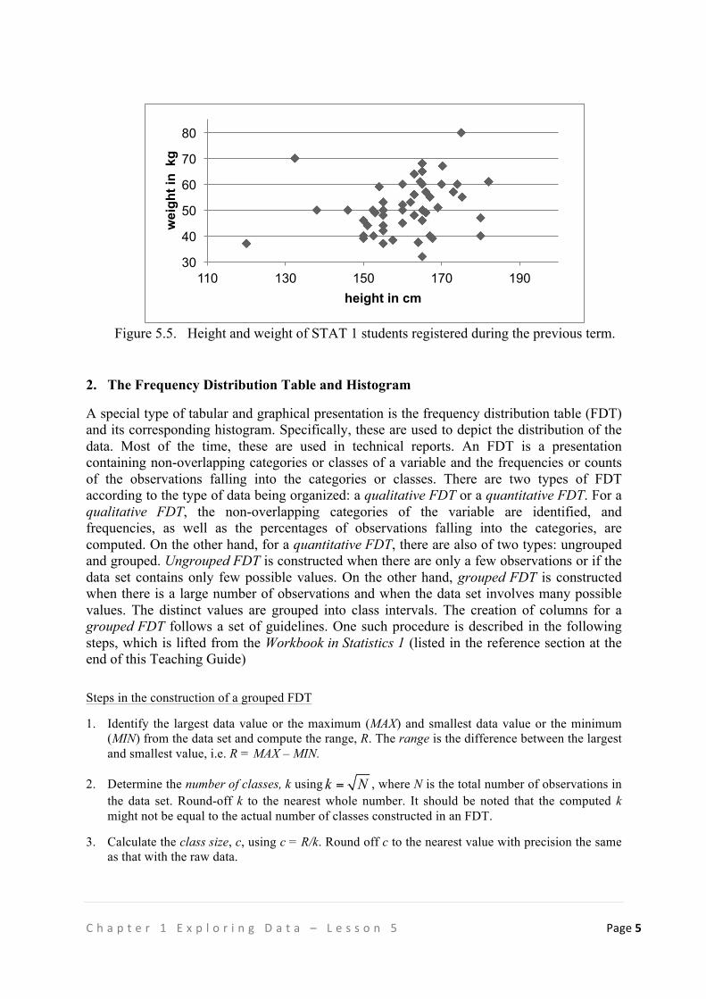
!C h a p t e r ! 1 ! E x p l o r i n g ! D a t a ! – ! L e s s o n ! 5 ! Page!5"! !!!!
Figure 5.5. Height and weight of STAT 1 students registered during the previous term.
2. The Frequency Distribution Table and Histogram
A special type of tabular and graphical presentation is the frequency distribution table (FDT) and its corresponding histogram. Specifically, these are used to depict the distribution of the data. Most of the time, these are used in technical reports. An FDT is a presentation containing non-overlapping categories or classes of a variable and the frequencies or counts of the observations falling into the categories or classes. There are two types of FDT according to the type of data being organized: a qualitative FDT or a quantitative FDT. For a qualitative FDT, the non-overlapping categories of the variable are identified, and frequencies, as well as the percentages of observations falling into the categories, are computed. On the other hand, for a quantitative FDT, there are also of two types: ungrouped and grouped. Ungrouped FDT is constructed when there are only a few observations or if the data set contains only few possible values. On the other hand, grouped FDT is constructed when there is a large number of observations and when the data set involves many possible values. The distinct values are grouped into class intervals. The creation of columns for a grouped FDT follows a set of guidelines. One such procedure is described in the following steps, which is lifted from the Workbook in Statistics 1 (listed in the reference section at the end of this Teaching Guide)
Steps in the construction of a grouped FDT 1. Identify the largest data value or the maximum (MAX) and smallest data value or the minimum
(MIN) from the data set and compute the range, R. The range is the difference between the largest and smallest value, i.e. R = MAX – MIN.
2. Determine the number of classes, k using k N= , where N is the total number of observations in the data set. Round-off k to the nearest whole number. It should be noted that the computed k might not be equal to the actual number of classes constructed in an FDT.
3. Calculate the class size, c, using c = R/k. Round off c to the nearest value with precision the same
as that with the raw data.
30
40
50
60
70
80
110 130 150 170 190
wei
ght i
n k
g
height in cm
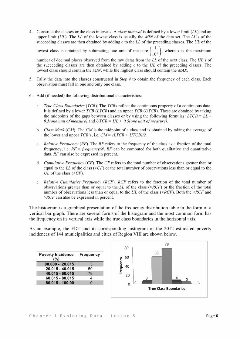
!C h a p t e r ! 1 ! E x p l o r i n g ! D a t a ! – ! L e s s o n ! 5 ! Page!6"! !!!!
4. Construct the classes or the class intervals. A class interval is defined by a lower limit (LL) and an upper limit (UL). The LL of the lowest class is usually the MIN of the data set. The LL’s of the succeeding classes are then obtained by adding c to the LL of the preceding classes. The UL of the
lowest class is obtained by subtracting one unit of measure 110x! "# $% &
, where x is the maximum
number of decimal places observed from the raw data) from the LL of the next class. The UL’s of the succeeding classes are then obtained by adding c to the UL of the preceding classes. The lowest class should contain the MIN, while the highest class should contain the MAX.
5. Tally the data into the classes constructed in Step 4 to obtain the frequency of each class. Each
observation must fall in one and only one class. !
6. Add (if needed) the following distributional characteristics:
a. True Class Boundaries (TCB). The TCBs reflect the continuous property of a continuous data. It is defined by a lower TCB (LTCB) and an upper TCB (UTCB). These are obtained by taking the midpoints of the gaps between classes or by using the following formulas: LTCB = LL – 0.5(one unit of measure) and UTCB = UL + 0.5(one unit of measure).
b. Class Mark (CM). The CM is the midpoint of a class and is obtained by taking the average of
the lower and upper TCB’s, i.e. CM = (LTCB + UTCB)/2. c. Relative Frequency (RF). The RF refers to the frequency of the class as a fraction of the total
frequency, i.e. RF = frequency/N. RF can be computed for both qualitative and quantitative data. RF can also be expressed in percent.
d. Cumulative Frequency (CF). The CF refers to the total number of observations greater than or
equal to the LL of the class (>CF) or the total number of observations less than or equal to the UL of the class (<CF).
e. Relative Cumulative Frequency (RCF). RCF refers to the fraction of the total number of
observations greater than or equal to the LL of the class (>RCF) or the fraction of the total number of observations less than or equal to the UL of the class (<RCF). Both the <RCF and >RCF can also be expressed in percent.
The histogram is a graphical presentation of the frequency distribution table in the form of a vertical bar graph. There are several forms of the histogram and the most common form has the frequency on its vertical axis while the true class boundaries in the horizontal axis.
As an example, the FDT and its corresponding histogram of the 2012 estimated poverty incidences of 144 municipalities and cities of Region VIII are shown below.
Poverty Incidence (%)
Frequency
00.000 - 20.015 3 20.015 - 40.015 59 40.015 - 60.015 78 60.015 - 80.015 4 80.015 - 100.00 0
0!
20!
40!
60!
80!
3!
59!
78!
4! 0!
Freq
uency"
True"Class"Boundaries"
!C h a p t e r ! 1 ! E x p l o r i n g ! D a t a ! – ! L e s s o n ! 5 ! Page!7"! !!!!
KEY POINTS
• Three methods of data presentation: textual, tabular and graphical • Two or all the methods could be combined to fully describe the data at hand. • Distribution of data is presented using frequency distribution table and histogram.
REFERENCES
Albert, J. R. G. (2008). Basic Statistics for the Tertiary Level (ed. Roberto Padua, Welfredo Patungan, Nelia Marquez), published by Rex Bookstore.
Handbook of Statistics 1 (1st and 2nd Edition), Authored by the Faculty of the Institute of Statistics, UP Los Baños, College Laguna 4031
Takahashi, S. (2009). The Manga Guide to Statistics. Trend-Pro Co. Ltd.
Workbooks in Statistics 1 (From 1st to 13th Edition), Authored by the Faculty of the Institute of Statistics, UP Los Baños, College Laguna 4031
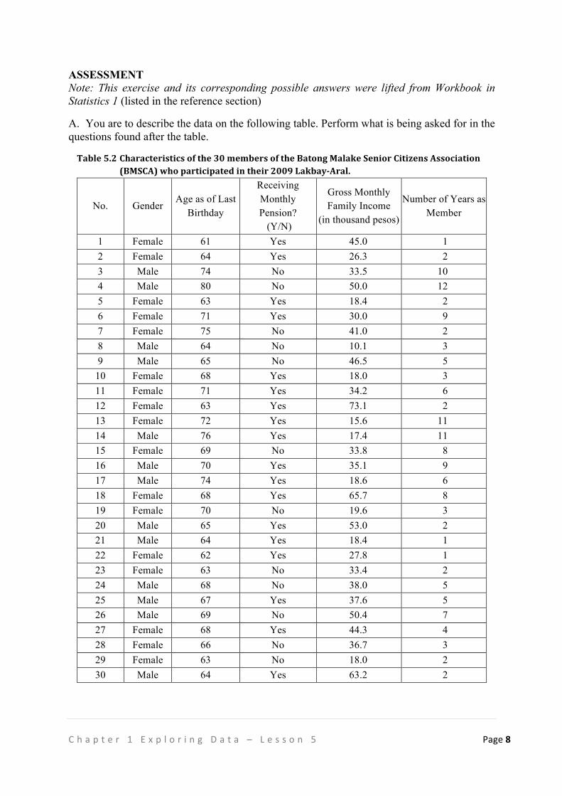
!C h a p t e r ! 1 ! E x p l o r i n g ! D a t a ! – ! L e s s o n ! 5 ! Page!8"! !!!!
ASSESSMENT Note: This exercise and its corresponding possible answers were lifted from Workbook in Statistics 1 (listed in the reference section)
A. You are to describe the data on the following table. Perform what is being asked for in the questions found after the table.
!!!!Table!5.2!!Characteristics!of!the!30!members!of!the!Batong!Malake!Senior!Citizens!Association!(BMSCA)!who!participated!in!their!2009!LakbayFAral.!
No. Gender Age as of Last
Birthday
Receiving Monthly Pension? (Y/N)
Gross Monthly Family Income
(in thousand pesos)
Number of Years as Member
1 Female 61 Yes 45.0 1 2 Female 64 Yes 26.3 2 3 Male 74 No 33.5 10 4 Male 80 No 50.0 12 5 Female 63 Yes 18.4 2 6 Female 71 Yes 30.0 9 7 Female 75 No 41.0 2 8 Male 64 No 10.1 3 9 Male 65 No 46.5 5
10 Female 68 Yes 18.0 3 11 Female 71 Yes 34.2 6 12 Female 63 Yes 73.1 2 13 Female 72 Yes 15.6 11 14 Male 76 Yes 17.4 11 15 Female 69 No 33.8 8 16 Male 70 Yes 35.1 9 17 Male 74 Yes 18.6 6 18 Female 68 Yes 65.7 8 19 Female 70 No 19.6 3 20 Male 65 Yes 53.0 2 21 Male 64 Yes 18.4 1 22 Female 62 Yes 27.8 1 23 Female 63 No 33.4 2 24 Male 68 No 38.0 5 25 Male 67 Yes 37.6 5 26 Male 69 No 50.4 7 27 Female 68 Yes 44.3 4 28 Female 66 No 36.7 3 29 Female 63 No 18.0 2 30 Male 64 Yes 63.2 2 !
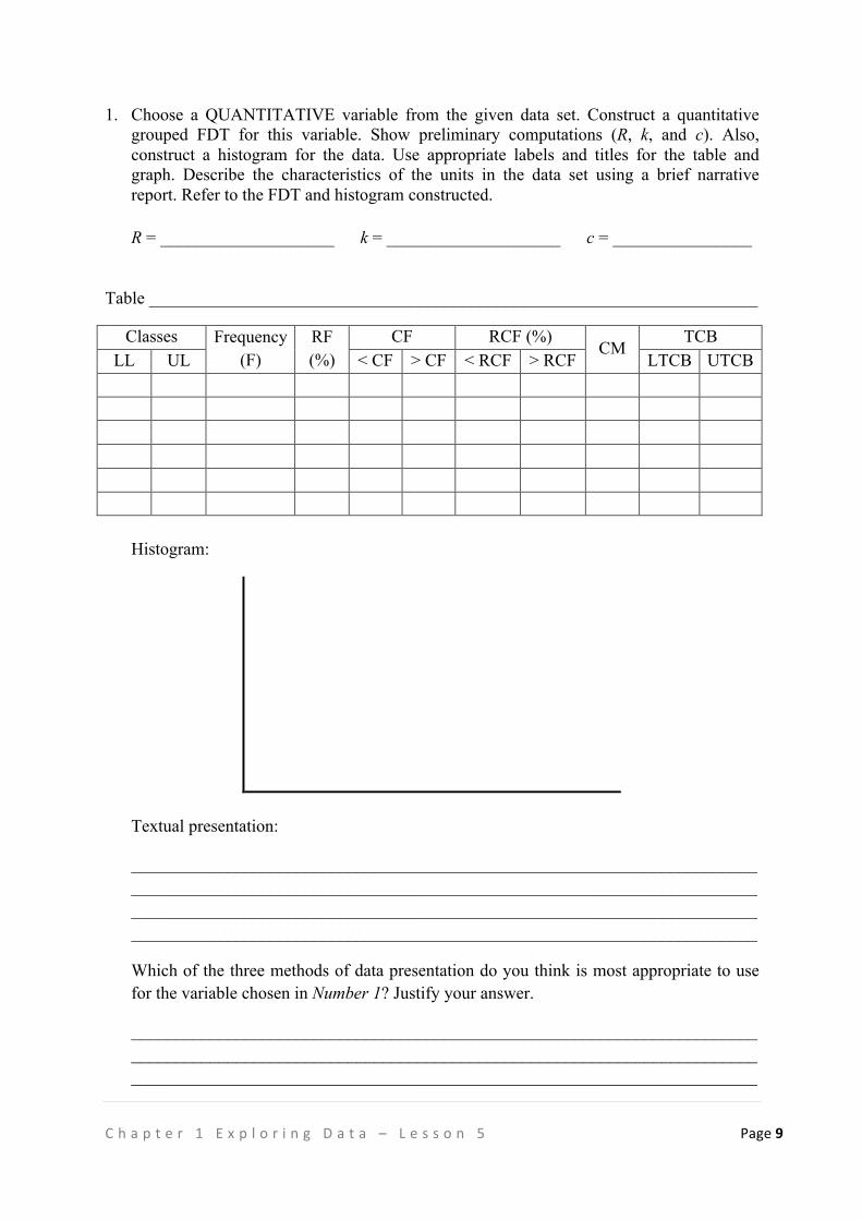
!C h a p t e r ! 1 ! E x p l o r i n g ! D a t a ! – ! L e s s o n ! 5 ! Page!9"! !!!!
1. Choose a QUANTITATIVE variable from the given data set. Construct a quantitative grouped FDT for this variable. Show preliminary computations (R, k, and c). Also, construct a histogram for the data. Use appropriate labels and titles for the table and graph. Describe the characteristics of the units in the data set using a brief narrative report. Refer to the FDT and histogram constructed.
R = ____________________ k = ____________________ c = ________________
Table ______________________________________________________________________
Classes Frequency (F)
RF (%)
CF RCF (%) CM
TCB LL UL < CF > CF < RCF > RCF LTCB UTCB
Histogram:
Textual presentation:
________________________________________________________________________ ________________________________________________________________________ ________________________________________________________________________ ________________________________________________________________________
Which of the three methods of data presentation do you think is most appropriate to use for the variable chosen in Number 1? Justify your answer.
________________________________________________________________________________________________________________________________________________________________________________________________________________________
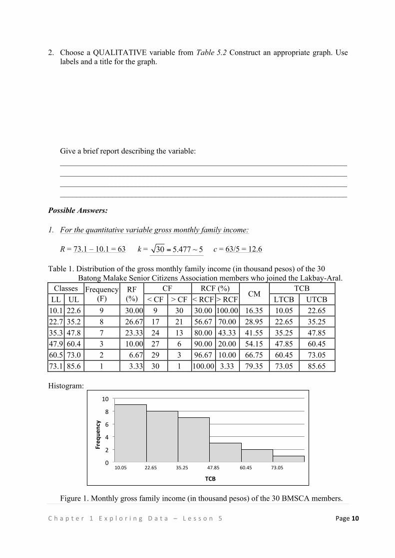
!C h a p t e r ! 1 ! E x p l o r i n g ! D a t a ! – ! L e s s o n ! 5 ! Page!10"! !!!!
2. Choose a QUALITATIVE variable from Table 5.2 Construct an appropriate graph. Use labels and a title for the graph.
Give a brief report describing the variable: ________________________________________________________________________ ________________________________________________________________________ ________________________________________________________________________ ________________________________________________________________________
Possible Answers: 1. For the quantitative variable gross monthly family income:
R = 73.1 – 10.1 = 63 k = 30 5.477 ~ 5= c = 63/5 = 12.6
Table 1. Distribution of the gross monthly family income (in thousand pesos) of the 30 Batong Malake Senior Citizens Association members who joined the Lakbay-Aral.
Classes Frequency (F)
RF (%)
CF RCF (%) CM
TCB LL UL < CF > CF < RCF > RCF LTCB UTCB
10.1 22.6 9 30.00 9 30 30.00 100.00 16.35 10.05 22.65 22.7 35.2 8 26.67 17 21 56.67 70.00 28.95 22.65 35.25 35.3 47.8 7 23.33 24 13 80.00 43.33 41.55 35.25 47.85 47.9 60.4 3 10.00 27 6 90.00 20.00 54.15 47.85 60.45 60.5 73.0 2 6.67 29 3 96.67 10.00 66.75 60.45 73.05 73.1 85.6 1 3.33 30 1 100.00 3.33 79.35 73.05 85.65 Histogram:
!
Figure 1. Monthly gross family income (in thousand pesos) of the 30 BMSCA members.
0!
2!
4!
6!
8!
10!
1! 2! 3! 4! 5! 6!
Freq
uency"
TCB"
10.05!!!!!!!!!!!!!!!22.65!!!!!!!!!!!!!!!!35.25!!!!!!!!!!!!!!!!47.85!!!!!!!!!!!!!!!!!60.45!!!!!!!!!!!!!!!!73.05!!!!!!!!!!!!!!!!!85.65!
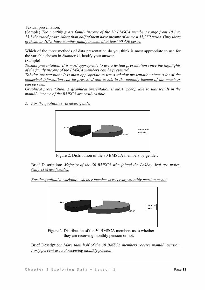
!C h a p t e r ! 1 ! E x p l o r i n g ! D a t a ! – ! L e s s o n ! 5 ! Page!11"! !!!!
Textual presentation: (Sample) The monthly gross family income of the 30 BMSCA members range from 10.1 to 73.1 thousand pesos. More than half of them have income of at most 35,250 pesos. Only three of them, or 10%, have monthly family income of at least 60,450 pesos. Which of the three methods of data presentation do you think is most appropriate to use for the variable chosen in Number 1? Justify your answer. (Sample) Textual presentation: It is most appropriate to use a textual presentation since the highlights of the family income of the BMSCA members can be presented. Tabular presentation: It is most appropriate to use a tabular presentation since a lot of the numerical information can be presented and trends in the monthly income of the members can be seen. Graphical presentation: A graphical presentation is most appropriate so that trends in the monthly income of the BMSCA are easily visible. 2. For the qualitative variable: gender
!! Figure 2. Distribution of the 30 BMSCA members by gender. ! !
Brief Description: Majority of the 30 BMSCA who joined the Lakbay-Aral are males. Only 43% are females. For the qualitative variable: whether member is receiving monthly pension or not
! Figure 2. Distribution of the 30 BMSCA members as to whether
they are receiving monthly pension or not. Brief Description: More than half of the 30 BMSCA members receive monthly pension. Forty percent are not receiving monthly pension.
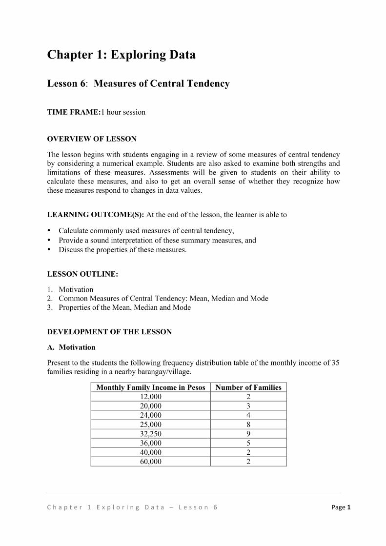
!C h a p t e r ! 1 ! E x p l o r i n g ! D a t a ! – ! L e s s o n ! 6 ! Page!1"! !!!!
Chapter 1: Exploring Data Lesson 6: Measures of Central Tendency
TIME FRAME:1 hour session OVERVIEW OF LESSON
The lesson begins with students engaging in a review of some measures of central tendency by considering a numerical example. Students are also asked to examine both strengths and limitations of these measures. Assessments will be given to students on their ability to calculate these measures, and also to get an overall sense of whether they recognize how these measures respond to changes in data values.
LEARNING OUTCOME(S): At the end of the lesson, the learner is able to
• Calculate commonly used measures of central tendency, • Provide a sound interpretation of these summary measures, and • Discuss the properties of these measures.
LESSON OUTLINE:
1. Motivation 2. Common Measures of Central Tendency: Mean, Median and Mode 3. Properties of the Mean, Median and Mode
DEVELOPMENT OF THE LESSON
A. Motivation
Present to the students the following frequency distribution table of the monthly income of 35 families residing in a nearby barangay/village.
Monthly Family Income in Pesos Number of Families 12,000 2 20,000 3 24,000 4 25,000 8 32,250 9 36,000 5 40,000 2 60,000 2
!C h a p t e r ! 1 ! E x p l o r i n g ! D a t a ! – ! L e s s o n ! 6 ! Page!2"! !!!!
You may ask the students the following to pick up their interest and at the same time introduce to them some summary statistics.
1. What is the highest monthly family income? Lowest?
Answer: Highest monthly family income is 60,000 pesos while the lowest is 12,000
pesos. You may emphasize that the highest and lowest values, which are commonly known as maximum and minimum, respectively are summary measures of a data set. They represent important location values in the distribution of the data. However, these measures do not give a measure of location in the center of the distribution. 2. What monthly family income is most frequent in the village?
Answer: Monthly family income that is most frequent is 32,250 pesos.
The value of 32,250 occurs most often or it is the value with the highest frequency. This is called the modal value or simply the mode. In this data set, the value of 32,250 is found in the center of the distribution.
3. If you list down individually the values of the monthly family income from lowest to highest, what is the monthly family income where half of the total number of families have monthly family income less than or equal to that value while the other half have monthly family income greater than that value?
Answer: When arranged in increasing order or the data come in an array as in the following:
12,000; 12,000; 20,000; 20,000; 20,000; 24,000; 24,000; 24,000; 24,000; 25,000; 25,000;25,000; 25,000; 25,000; 25,000; 25,000; 25,000; 32,250; 32,250; 32,250; 32,250; 32,250; 32,250; 32,250; 32,250; 32,250; 36,000; 36,000; 36,000; 36,000; 36,000; 40,000; 40,000; 60,000; 60,000; there are 17 values that are less than the middle value while another 17 values are higher or equal to the middle value. That middle value is the 18th observation and it is equal to 32,250 pesos. The middle value is called the median and is found in the center of the distribution.
4. What is the average monthly family income?
Answer: When computed using the data values, the average is 30,007.14 pesos.
The average monthly family income is commonly referred to as the arithmetic mean or simply the mean which is computed by adding all the values and then the sum is divided by
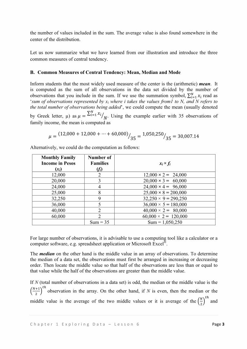
!C h a p t e r ! 1 ! E x p l o r i n g ! D a t a ! – ! L e s s o n ! 6 ! Page!3"! !!!!
the number of values included in the sum. The average value is also found somewhere in the center of the distribution. Let us now summarize what we have learned from our illustration and introduce the three common measures of central tendency. B. Common Measures of Central Tendency: Mean, Median and Mode Inform students that the most widely used measure of the center is the (arithmetic) mean. It is computed as the sum of all observations in the data set divided by the number of observations that you include in the sum. If we use the summation symbol, !!!
!!! read as ‘sum of observations represented by xi where i takes the values from1 to N, and N refers to the total number of observations being added’, we could compute the mean (usually denoted
by Greek letter, µ) as ! = !!!!!! !. Using the example earlier with 35 observations of
family income, the mean is computed as
! = 12,000+ 12,000+⋯+ 60,00035 =
1,050,25035 = 30,007.14
Alternatively, we could do the computation as follows:
Monthly Family Income in Pesos
(xi)
Number of Families
(fi)
xi × fi
12,000 2 12,000 × 2 = 24,000 20,000 3 20,000 × 3 = 60,000 24,000 4 24,000 × 4 = 96,000 25,000 8 25,000 × 8 = 200,000 32,250 9 32,250 × 9 = 290,250 36,000 5 36,000 × 5 = 180,000 40,000 2 40,000 × 2 = 80,000 60,000 2 60,000 × 2 = 120,000
Sum = 35 Sum = 1,050,250
For large number of observations, it is advisable to use a computing tool like a calculator or a computer software, e.g. spreadsheet application or Microsoft Excel®.
The median on the other hand is the middle value in an array of observations. To determine the median of a data set, the observations must first be arranged in increasing or decreasing order. Then locate the middle value so that half of the observations are less than or equal to that value while the half of the observations are greater than the middle value. If N (total number of observations in a data set) is odd, the median or the middle value is the !!!!
!!!observation in the array. On the other hand, if N is even, then the median or the
middle value is the average of the two middle values or it is average of the !!
!! and
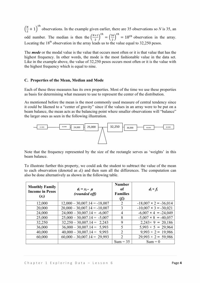
!C h a p t e r ! 1 ! E x p l o r i n g ! D a t a ! – ! L e s s o n ! 6 ! Page!4"! !!!!
!! + 1
!!!observations. In the example given earlier, there are 35 observations so N is 35, an
odd number. The median is then the !!!!
!!= !"
!!!= 18!! observation in the array.
Locating the 18th observation in the array leads us to the value equal to 32,250 pesos. The mode or the modal value is the value that occurs most often or it is that value that has the highest frequency. In other words, the mode is the most fashionable value in the data set. Like in the example above, the value of 32,250 pesos occurs most often or it is the value with the highest frequency which is equal to nine. C. Properties of the Mean, Median and Mode Each of these three measures has its own properties. Most of the time we use these properties as basis for determining what measure to use to represent the center of the distribution.
As mentioned before the mean is the most commonly used measure of central tendency since it could be likened to a “center of gravity” since if the values in an array were to be put on a beam balance, the mean acts as the balancing point where smaller observations will “balance” the larger ones as seen in the following illustration.
Note that the frequency represented by the size of the rectangle serves as ‘weights’ in this beam balance. To illustrate further this property, we could ask the student to subtract the value of the mean to each observation (denoted as di) and then sum all the differences. The computation can also be done alternatively as shown in the following table.
Monthly Family Income in Pesos
(xi)
di = xi - µ (rounded off)
Number of
Families (fi)
di × fi
12,000 12,000 – 30,007.14 = -18,007 2 -18,007 × 2 = -36,014 20,000 20,000 – 30,007.14 = -10,007 3 -10,007 × 3 = -30,021 24,000 24,000 – 30,007.14 = -6,007 4 -6,007 × 4 = -24,049 25,000 25,000 – 30,007.14 = -5,007 8 -5,007 × 8 = -40,057 32,250 32,250 – 30,007.14 = 2,243 9 2,243× 9 = 20,186 36,000 36,000 – 30,007.14 = 5,993 5 5,993 × 5 = 29,964 40,000 40,000 – 30,007.14 = 9,993 2 9,993 × 2 = 19,986 60,000 60,000 – 30,007.14 = 29,993 2 29,993 × 2 = 59,986
Sum = 35 Sum = 0
12,000! 20,000!
!24,000! 25,000! 32,250! 36,000! 40,000! 60,000!
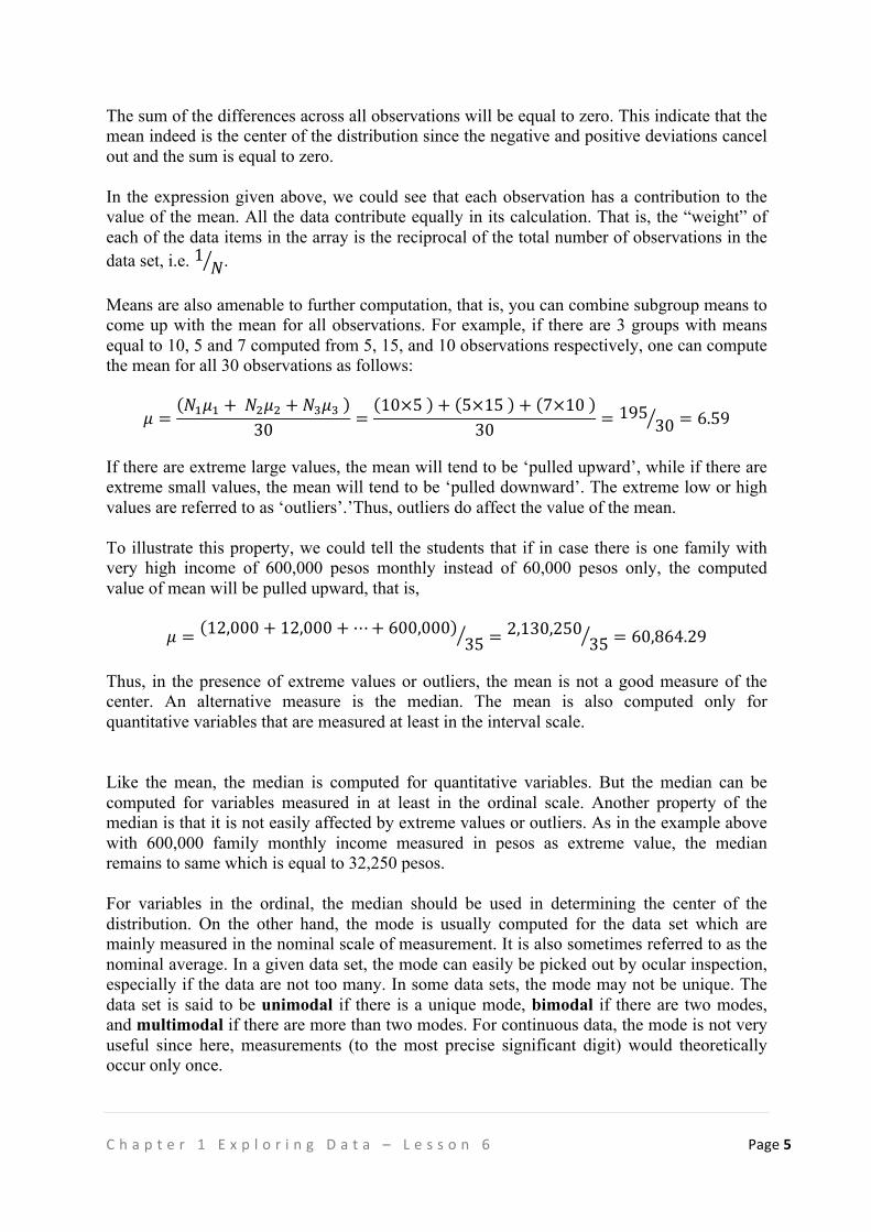
!C h a p t e r ! 1 ! E x p l o r i n g ! D a t a ! – ! L e s s o n ! 6 ! Page!5"! !!!!
The sum of the differences across all observations will be equal to zero. This indicate that the mean indeed is the center of the distribution since the negative and positive deviations cancel out and the sum is equal to zero. In the expression given above, we could see that each observation has a contribution to the value of the mean. All the data contribute equally in its calculation. That is, the “weight” of each of the data items in the array is the reciprocal of the total number of observations in the data set, i.e. 1 !. Means are also amenable to further computation, that is, you can combine subgroup means to come up with the mean for all observations. For example, if there are 3 groups with means equal to 10, 5 and 7 computed from 5, 15, and 10 observations respectively, one can compute the mean for all 30 observations as follows:
! = !!!! + !!!!! + !!!!!30 = 10×5! + 5×15! + 7×10!
30 = 195 30 = 6.59 If there are extreme large values, the mean will tend to be ‘pulled upward’, while if there are extreme small values, the mean will tend to be ‘pulled downward’. The extreme low or high values are referred to as ‘outliers’.’Thus, outliers do affect the value of the mean. To illustrate this property, we could tell the students that if in case there is one family with very high income of 600,000 pesos monthly instead of 60,000 pesos only, the computed value of mean will be pulled upward, that is,
! = 12,000+ 12,000+⋯+ 600,00035 =
2,130,25035 = 60,864.29
Thus, in the presence of extreme values or outliers, the mean is not a good measure of the center. An alternative measure is the median. The mean is also computed only for quantitative variables that are measured at least in the interval scale. Like the mean, the median is computed for quantitative variables. But the median can be computed for variables measured in at least in the ordinal scale. Another property of the median is that it is not easily affected by extreme values or outliers. As in the example above with 600,000 family monthly income measured in pesos as extreme value, the median remains to same which is equal to 32,250 pesos. For variables in the ordinal, the median should be used in determining the center of the distribution. On the other hand, the mode is usually computed for the data set which are mainly measured in the nominal scale of measurement. It is also sometimes referred to as the nominal average. In a given data set, the mode can easily be picked out by ocular inspection, especially if the data are not too many. In some data sets, the mode may not be unique. The data set is said to be unimodal if there is a unique mode, bimodal if there are two modes, and multimodal if there are more than two modes. For continuous data, the mode is not very useful since here, measurements (to the most precise significant digit) would theoretically occur only once.
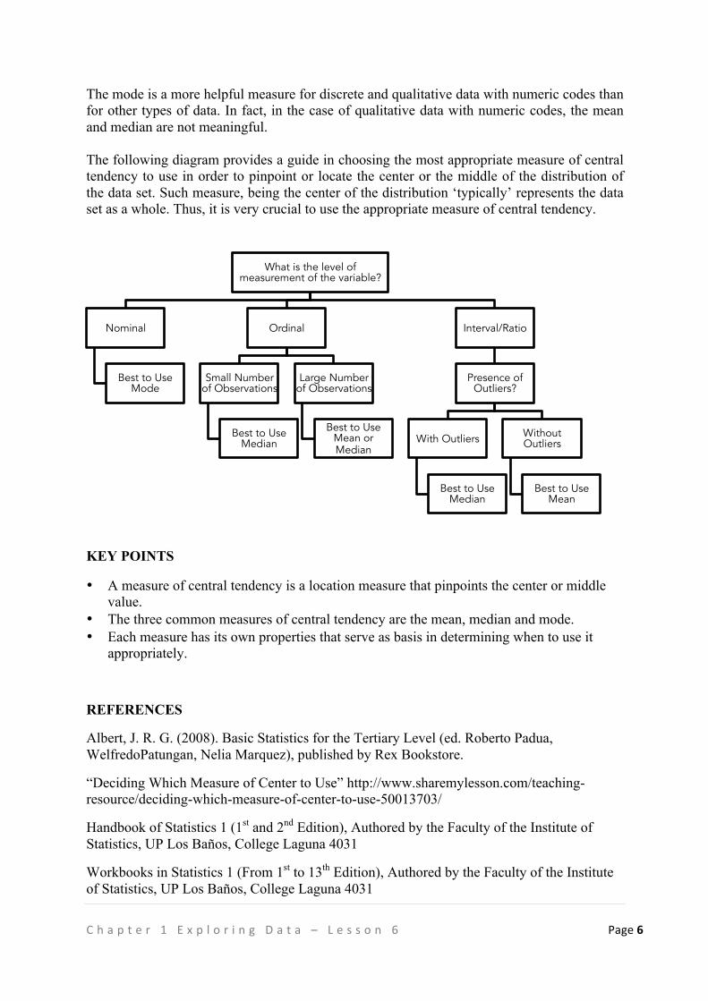
!C h a p t e r ! 1 ! E x p l o r i n g ! D a t a ! – ! L e s s o n ! 6 ! Page!6"! !!!!
The mode is a more helpful measure for discrete and qualitative data with numeric codes than for other types of data. In fact, in the case of qualitative data with numeric codes, the mean and median are not meaningful. The following diagram provides a guide in choosing the most appropriate measure of central tendency to use in order to pinpoint or locate the center or the middle of the distribution of the data set. Such measure, being the center of the distribution ‘typically’ represents the data set as a whole. Thus, it is very crucial to use the appropriate measure of central tendency.
KEY POINTS
• A measure of central tendency is a location measure that pinpoints the center or middle value.
• The three common measures of central tendency are the mean, median and mode. • Each measure has its own properties that serve as basis in determining when to use it
appropriately.
REFERENCES
Albert, J. R. G. (2008). Basic Statistics for the Tertiary Level (ed. Roberto Padua, WelfredoPatungan, Nelia Marquez), published by Rex Bookstore.
“Deciding Which Measure of Center to Use” http://www.sharemylesson.com/teaching-resource/deciding-which-measure-of-center-to-use-50013703/
Handbook of Statistics 1 (1st and 2nd Edition), Authored by the Faculty of the Institute of Statistics, UP Los Baños, College Laguna 4031
Workbooks in Statistics 1 (From 1st to 13th Edition), Authored by the Faculty of the Institute of Statistics, UP Los Baños, College Laguna 4031
What is the level of measurement of the variable?
Nominal
Best to Use Mode
Ordinal
Small Number of Observations
Best to Use Median
Large Number of Observations
Best to Use Mean or Median
Interval/Ratio
Presence of Outliers?
With Outliers
Best to Use Median
Without Outliers
Best to Use Mean
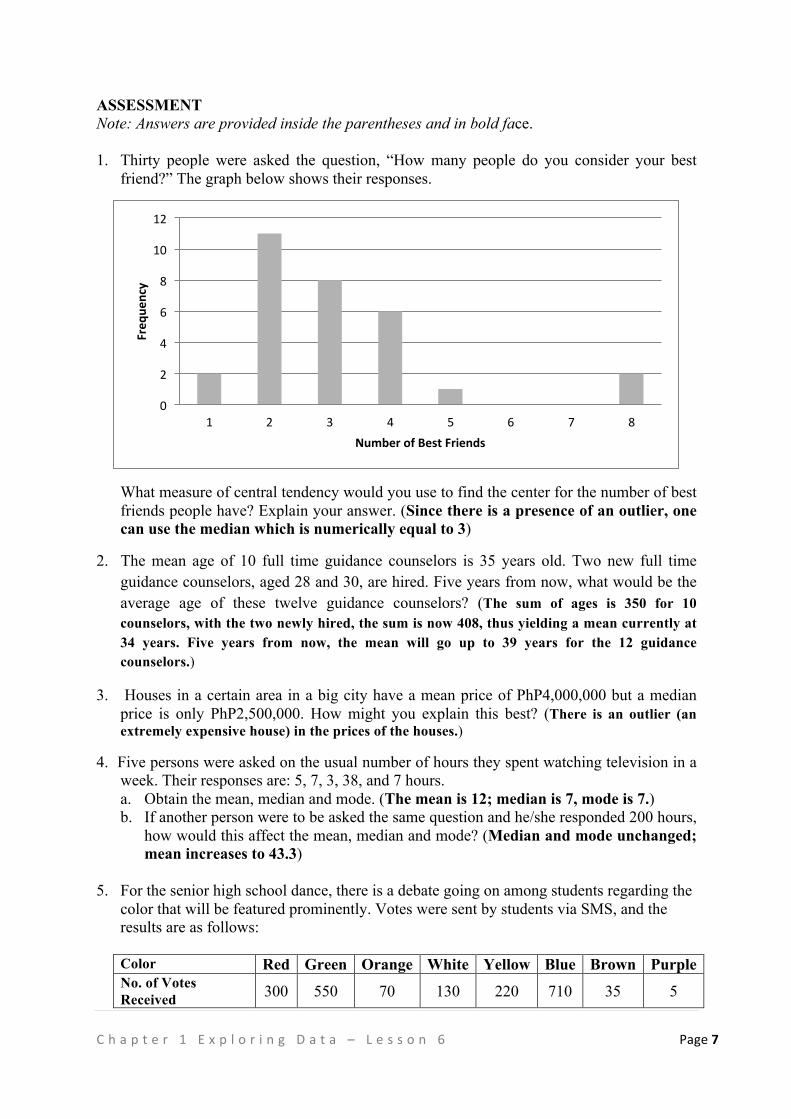
!C h a p t e r ! 1 ! E x p l o r i n g ! D a t a ! – ! L e s s o n ! 6 ! Page!7"! !!!!
ASSESSMENT Note: Answers are provided inside the parentheses and in bold face. 1. Thirty people were asked the question, “How many people do you consider your best
friend?” The graph below shows their responses.
What measure of central tendency would you use to find the center for the number of best friends people have? Explain your answer. (Since there is a presence of an outlier, one can use the median which is numerically equal to 3)
2. The mean age of 10 full time guidance counselors is 35 years old. Two new full time guidance counselors, aged 28 and 30, are hired. Five years from now, what would be the average age of these twelve guidance counselors? (The sum of ages is 350 for 10 counselors, with the two newly hired, the sum is now 408, thus yielding a mean currently at 34 years. Five years from now, the mean will go up to 39 years for the 12 guidance counselors.)
3. Houses in a certain area in a big city have a mean price of PhP4,000,000 but a median price is only PhP2,500,000. How might you explain this best? (There is an outlier (an extremely expensive house) in the prices of the houses.)
4. Five persons were asked on the usual number of hours they spent watching television in a week. Their responses are: 5, 7, 3, 38, and 7 hours. a. Obtain the mean, median and mode. (The mean is 12; median is 7, mode is 7.) b. If another person were to be asked the same question and he/she responded 200 hours,
how would this affect the mean, median and mode? (Median and mode unchanged; mean increases to 43.3)
5. For the senior high school dance, there is a debate going on among students regarding the color that will be featured prominently. Votes were sent by students via SMS, and the results are as follows: Color Red Green Orange White Yellow Blue Brown Purple No. of Votes Received 300 550 70 130 220 710 35 5
0!
2!
4!
6!
8!
10!
12!
1! 2! 3! 4! 5! 6! 7! 8!
Freq
uency"
Number"of"Best"Friends"
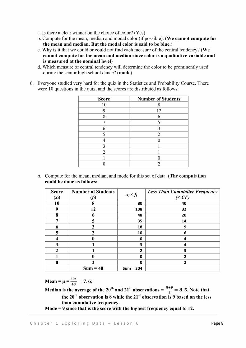
!C h a p t e r ! 1 ! E x p l o r i n g ! D a t a ! – ! L e s s o n ! 6 ! Page!8"! !!!!
a. Is there a clear winner on the choice of color? (Yes) b. Compute for the mean, median and modal color (if possible). (We cannot compute for
the mean and median. But the modal color is said to be blue.) c. Why is it that we could or could not find each measure of the central tendency? (We
cannot compute for the mean and median since color is a qualitative variable and is measured at the nominal level)
d. Which measure of central tendency will determine the color to be prominently used during the senior high school dance? (mode)
6. Everyone studied very hard for the quiz in the Statistics and Probability Course. There
were 10 questions in the quiz, and the scores are distributed as follows:
Score Number of Students 10 8 9 12 8 6 7 5 6 3 5 2 4 0 3 1 2 1 1 0 0 2
a. Compute for the mean, median, and mode for this set of data. (The computation
could be done as follows:
Score (xi)
Number of Students (fi)
xi × fi Less Than Cumulative Frequency
(< CF) 10 8 80" 40"9 12 108" 32"8 6 48" 20"7 5 35" 14"6 3 18" 9"5 2 10" 6"4 0 0" 4"3 1 3" 4"2 1 2" 3"1 0 0" 2"0 2 0" 2" Sum = 40 Sum"="304" "
Mean = µ = !"#!" = !.!;
Median is the average of the 20th and 21st observations = !!!! = !.!. Note that the 20th observation is 8 while the 21st observation is 9 based on the less than cumulative frequency.
Mode = 9 since that is the score with the highest frequency equal to 12.
!C h a p t e r ! 1 ! E x p l o r i n g ! D a t a ! – ! L e s s o n ! 6 ! Page!9"! !!!!
c. Suppose the teacher said “Everyone in the class will be getting either the mean,
median, or mode for their official score.” i. What would students want to receive (mean, median, or mode)? (Mode) ii. Which would students want to receive the least (mean, median or mode)? (Mean) iii What is the fairest score to receive would be? Ask students to explain their
answers. (Note: There is no right or wrong answer for this question. It all depends on the reasoning of the students)
!C h a p t e r ! 1 ! E x p l o r i n g ! D a t a ! – ! L e s s o n ! 7 ! Page!1"! !!!!
Chapter 1: Exploring Data Lesson 7: Other Measures of Location
TIME FRAME:1 hour session OVERVIEW OF LESSON
In the previous lesson we discussed a measure of location known as the measure of central tendency. There are other measures of location which are useful in describing the distribution of the data set. These measures of location include the maximum, minimum, percentiles, deciles and quartiles. How to compute and interpret these measures are also discussed in this lesson.
LEARNING OUTCOME(S): At the end of the lesson, the learner is able to
• Calculate measures of location other than the measure of central tendency, and • Provide a sound interpretation of these summary measures.
LESSON OUTLINE:
1. Motivation 2. Measures of Location: Maximum, Minimum, Percentiles, Deciles and Quartiles
DEVELOPMENT OF THE LESSON
A. Motivation
In the previous lesson, we ask the students to identify the highest and lowest family income, and emphasized that that the highest and the lowest values, which are commonly known as maximum and minimum, respectively are important summary measures of a data set. They represent important location values in the distribution of the data. However, these measures do not give a measure of location in the center of the distribution. Instead, these two location measures give extreme locations or points in a distribution.
For example, after a long test or examination, we are interested what is the highest score or lowest score and of course who got these scores. These are in addition to knowing the average, median and modal scores. These measures tell us how the students perform in the long test. Knowing these measures, we could do further actions like reward the student(s) who got the highest score and assist those student(s) who got the lowest score. In addition, these measures also indicate if the long test is difficult or easy and the measures may also indicate the level of understanding of the students in the concepts that are covered in the test.
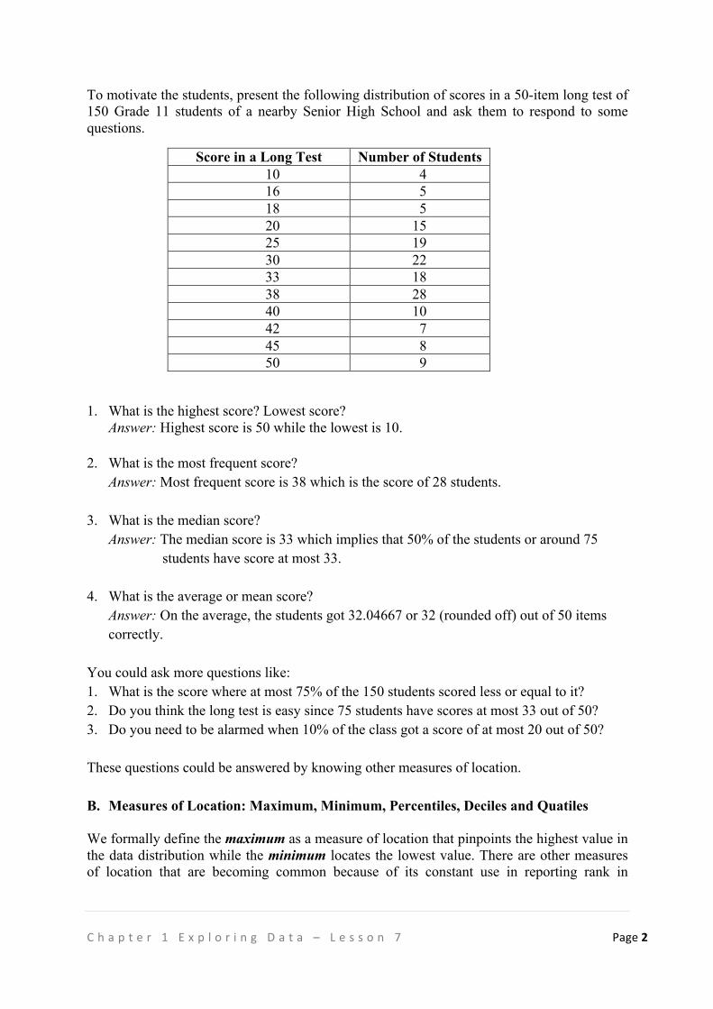
!C h a p t e r ! 1 ! E x p l o r i n g ! D a t a ! – ! L e s s o n ! 7 ! Page!2"! !!!!
To motivate the students, present the following distribution of scores in a 50-item long test of 150 Grade 11 students of a nearby Senior High School and ask them to respond to some questions.
Score in a Long Test Number of Students 10 4 16 5 18 5 20 15 25 19 30 22 33 18 38 28 40 10 42 7 45 8 50 9
1. What is the highest score? Lowest score? Answer: Highest score is 50 while the lowest is 10.
2. What is the most frequent score?
Answer: Most frequent score is 38 which is the score of 28 students.
3. What is the median score? Answer: The median score is 33 which implies that 50% of the students or around 75
students have score at most 33.
4. What is the average or mean score? Answer: On the average, the students got 32.04667 or 32 (rounded off) out of 50 items correctly.
You could ask more questions like: 1. What is the score where at most 75% of the 150 students scored less or equal to it? 2. Do you think the long test is easy since 75 students have scores at most 33 out of 50? 3. Do you need to be alarmed when 10% of the class got a score of at most 20 out of 50? These questions could be answered by knowing other measures of location. B. Measures of Location: Maximum, Minimum, Percentiles, Deciles and Quatiles We formally define the maximum as a measure of location that pinpoints the highest value in the data distribution while the minimum locates the lowest value. There are other measures of location that are becoming common because of its constant use in reporting rank in
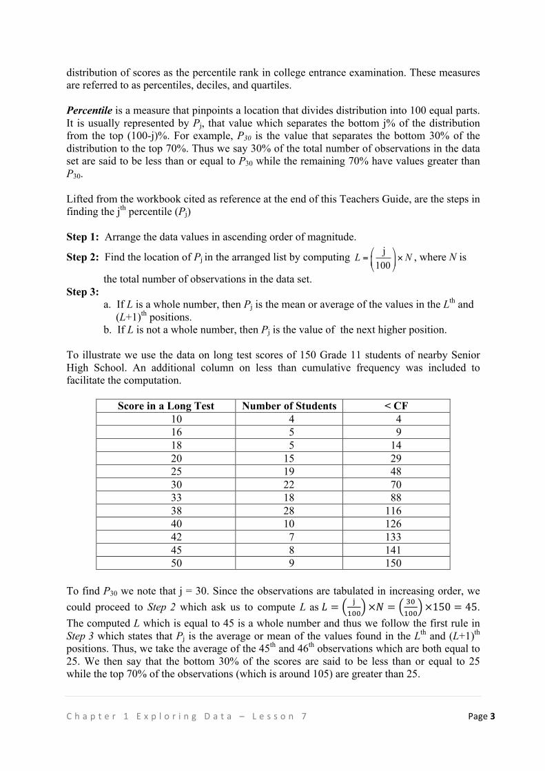
!C h a p t e r ! 1 ! E x p l o r i n g ! D a t a ! – ! L e s s o n ! 7 ! Page!3"! !!!!
distribution of scores as the percentile rank in college entrance examination. These measures are referred to as percentiles, deciles, and quartiles. Percentile is a measure that pinpoints a location that divides distribution into 100 equal parts. It is usually represented by Pj, that value which separates the bottom j% of the distribution from the top (100-j)%. For example, P30 is the value that separates the bottom 30% of the distribution to the top 70%. Thus we say 30% of the total number of observations in the data set are said to be less than or equal to P30 while the remaining 70% have values greater than P30. Lifted from the workbook cited as reference at the end of this Teachers Guide, are the steps in finding the jth percentile (Pj) Step 1: Arrange the data values in ascending order of magnitude.
Step 2: Find the location of Pj in the arranged list by computing j100
L N! "= ×$ %& '
, where N is
the total number of observations in the data set. Step 3:
a. If L is a whole number, then Pj is the mean or average of the values in the Lth and (L+1)th positions.
b. If L is not a whole number, then Pj is the value of the next higher position. To illustrate we use the data on long test scores of 150 Grade 11 students of nearby Senior High School. An additional column on less than cumulative frequency was included to facilitate the computation.
Score in a Long Test Number of Students < CF 10 4 4 16 5 9 18 5 14 20 15 29 25 19 48 30 22 70 33 18 88 38 28 116 40 10 126 42 7 133 45 8 141 50 9 150
To find P30 we note that j = 30. Since the observations are tabulated in increasing order, we could proceed to Step 2 which ask us to compute L as ! = !
!"" ×! = !"!"" ×150 = 45.
The computed L which is equal to 45 is a whole number and thus we follow the first rule in Step 3 which states that Pj is the average or mean of the values found in the Lth and (L+1)th
positions. Thus, we take the average of the 45th and 46th observations which are both equal to 25. We then say that the bottom 30% of the scores are said to be less than or equal to 25 while the top 70% of the observations (which is around 105) are greater than 25.
!C h a p t e r ! 1 ! E x p l o r i n g ! D a t a ! – ! L e s s o n ! 7 ! Page!4"! !!!!
Deciles and quartiles are then defined in relation to percentile. If the percentile divides the distribution into 100 equal parts, deciles divide the distribution into 10 equal parts while quartiles divide the distribution into 4 equal parts. Thus, we say that 10th Percentile is the same as the 1st Decile, 20th Percentile same as 2nd Decile, 25th Percentile same as 1st Quartile, 50th Percentile same as 5th Decile or 2nd Quartile and so forth. Note also that by definition of the median in previous lesson, we could say that the median value is equal to the 50th Percentile or 5th Decile or 2nd Quartile. Because of this relationship, the computation of the quartile and decile could be coursed through the computation of the percentile.
To illustrate, if we want to compute the 3rd Decile or D3 then we compute 30th Percentile or P30. In other words, D3 = P30 = 25 based on our earlier computation. The 3rd Quartile or Q3 is equal to P75. To compute L as ! = !
!"" ×! = !"!"" ×150 = 112.5. The computed L which
is equal to 112.5 is not a whole number and thus we follow the second rule in Step 3 which states that Pj is the value found in the next higher position, specifically, in 113th position, the next higher position after 112.5. Thus, we take the 113th observation which is equal to 38 as the value of P75. We then say that 75% of the class of 150 students or around 113 students correctly answered at most 38 out of the 50 items.
The median which is equal to P50 is computed as the mean or average of the 75th and 76th observations which are both equal to 33. Hence, we did get the same value as the one we obtained using the definition we had in the previous lesson.
KEY POINTS • There are other measures of location that could further describe the distribution of the
data set. • The maximum and minimum values are measures of location that pinpoints the extreme
values which are the highest and lowest values, respectively. • Percentiles, quartiles and deciles are measures of locations that divide the distribution into
100, 4 and 10 equal parts, respectively.
REFERENCES “Deciding Which Measure of Center to Use” http://www.sharemylesson.com/teaching-resource/deciding-which-measure-of-center-to-use-50013703/
Albert, J. R. G. (2008). Basic Statistics for the Tertiary Level (ed. Roberto Padua, WelfredoPatungan, Nelia Marquez), published by Rex Bookstore.
Handbook of Statistics 1 (1st and 2nd Edition), Authored by the Faculty of the Institute of Statistics, UP Los Baños, College Laguna 4031
Moore, D.S. (2007). The Basic Practice of Statistics, Fourth Edition W.H. Freeman and Company.
Workbooks in Statistics 1 (From 1st to 13th Edition), Authored by the Faculty of the Institute of Statistics, UP Los Baños, College Laguna 4031
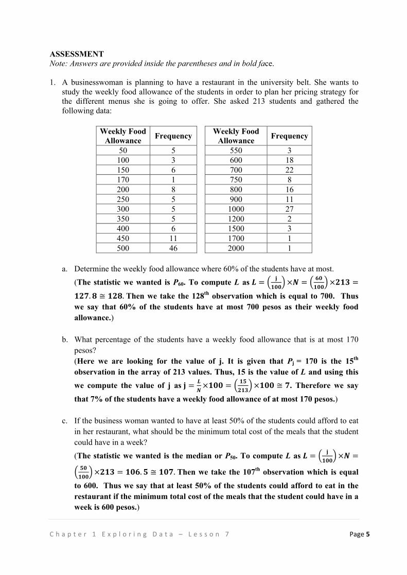
!C h a p t e r ! 1 ! E x p l o r i n g ! D a t a ! – ! L e s s o n ! 7 ! Page!5"! !!!!
ASSESSMENT Note: Answers are provided inside the parentheses and in bold face. 1. A businesswoman is planning to have a restaurant in the university belt. She wants to
study the weekly food allowance of the students in order to plan her pricing strategy for the different menus she is going to offer. She asked 213 students and gathered the following data:
Weekly Food Allowance Frequency Weekly Food
Allowance Frequency
50 5 550 3 100 3 600 18 150 6 700 22 170 1 750 8 200 8 800 16 250 5 900 11 300 5 1000 27 350 5 1200 2 400 6 1500 3 450 11 1700 1 500 46 2000 1
a. Determine the weekly food allowance where 60% of the students have at most.
(The statistic we wanted is P60. To compute L as ! = !!"" ×! = !"
!"" ×!"# =!"#.! ≅ !"#. Then we take the 128th observation which is equal to 700. Thus we say that 60% of the students have at most 700 pesos as their weekly food allowance.)
b. What percentage of the students have a weekly food allowance that is at most 170 pesos? (Here we are looking for the value of j. It is given that Pj = 170 is the 15th observation in the array of 213 values. Thus, 15 is the value of L and using this
we compute the value of j as ! = !!×!"" =
!"!"# ×!"" ≅ !. Therefore we say
that 7% of the students have a weekly food allowance of at most 170 pesos.)
c. If the business woman wanted to have at least 50% of the students could afford to eat in her restaurant, what should be the minimum total cost of the meals that the student could have in a week?
(The statistic we wanted is the median or P50. To compute L as ! = !!"" ×! =
!"!"" ×!"# = !"#.! ≅ !"#. Then we take the 107th observation which is equal
to 600. Thus we say that at least 50% of the students could afford to eat in the restaurant if the minimum total cost of the meals that the student could have in a week is 600 pesos.)
!C h a p t e r ! 1 ! E x p l o r i n g ! D a t a ! – ! L e s s o n ! 8 ! Page!1"! !!!!
Chapter 1: Exploring Data Lesson 8: Measures of Variation
TIME FRAME:1 hour session OVERVIEW OF LESSON
In this lesson, students will be shown that it is not enough to get measures of central tendency in a data set by scrutinizing two different data sets with the same measures of central tendency. We illustrate this using data on the returns on stocks where it is not only the mean, median and mode which are the same, it is also true for other measures of location like its minimum and maximum. However, the spread of observations are different which means that to further describe the data sets we need additional measures like a measure about the dispersion of the data, i.e. range, interquartile range, variance, standard deviation, and coefficient of variation. Also, the standard deviation, as a measure of dispersion can be viewed as a measure of risk, specifically in the case of making investments in stock market. The smaller the value of the standard deviation, the smaller is the risk.
LEARNING OUTCOME(S): At the end of the lesson, the learner is able to
• Calculate some measures of dispersion; • Think of the strengths and limitations of these measures; and • Provide a sound interpretation of these measures.
LESSON OUTLINE:
1. Introduction: The Case of the Returns on Stocks 2. Absolute Measures of Dispersion: Range, Interquartile Range, Variance, Standard
Deviation and Coefficient of Variation 3. Relative Measure of Dispersion: Coefficient of Variation
DEVELOPMENT OF THE LESSON
A. Introduction: The Case of the Returns on Stocks.
To introduce this lesson, tell the students the importance of thinking about their future, of saving, and of wealth generation. Explain that a number of people invest money into the stock market as an alternative financial instrument to generate wealth from savings.
Explanatory Note: Stocks are shares of ownership in a company. When people buy stocks they become part owners of the company, whether in terms of profits or losses of the company.
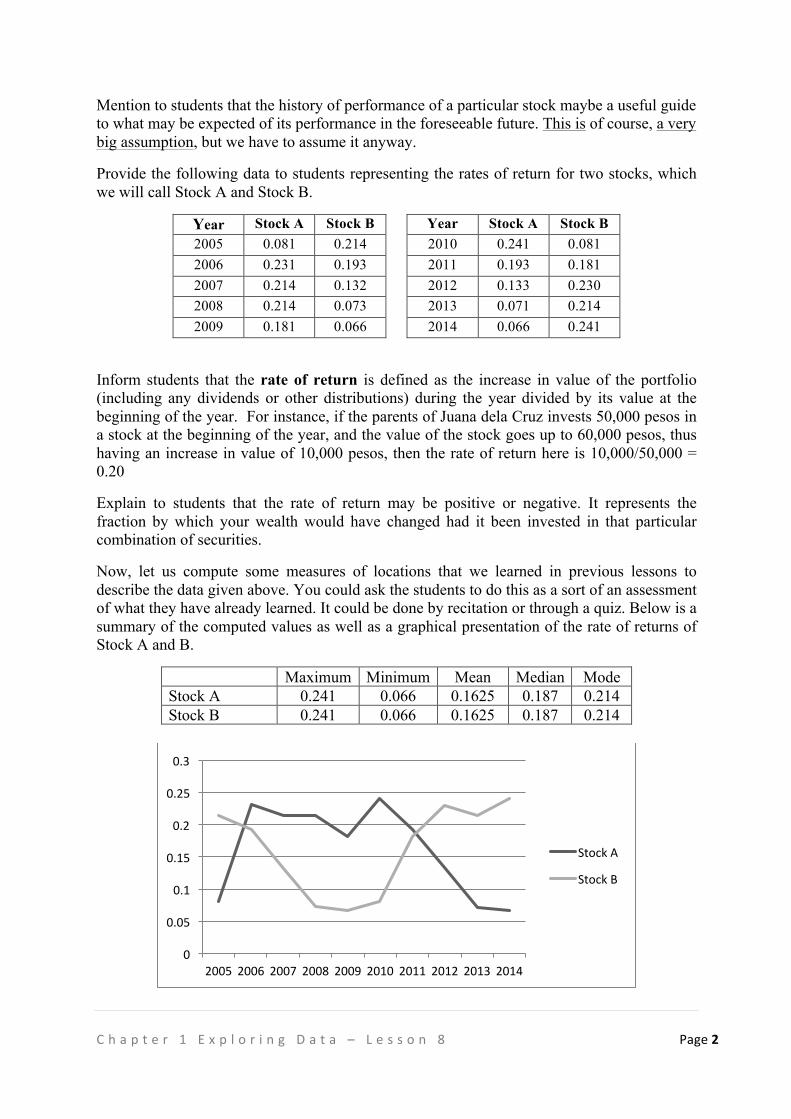
!C h a p t e r ! 1 ! E x p l o r i n g ! D a t a ! – ! L e s s o n ! 8 ! Page!2"! !!!!
Mention to students that the history of performance of a particular stock maybe a useful guide to what may be expected of its performance in the foreseeable future. This is of course, a very big assumption, but we have to assume it anyway.
Provide the following data to students representing the rates of return for two stocks, which we will call Stock A and Stock B.
Year Stock A Stock B Year Stock A Stock B 2005 0.081 0.214 2010 0.241 0.081 2006 0.231 0.193 2011 0.193 0.181 2007 0.214 0.132 2012 0.133 0.230 2008 0.214 0.073 2013 0.071 0.214 2009 0.181 0.066 2014 0.066 0.241
Inform students that the rate of return is defined as the increase in value of the portfolio (including any dividends or other distributions) during the year divided by its value at the beginning of the year. For instance, if the parents of Juana dela Cruz invests 50,000 pesos in a stock at the beginning of the year, and the value of the stock goes up to 60,000 pesos, thus having an increase in value of 10,000 pesos, then the rate of return here is 10,000/50,000 = 0.20
Explain to students that the rate of return may be positive or negative. It represents the fraction by which your wealth would have changed had it been invested in that particular combination of securities.
Now, let us compute some measures of locations that we learned in previous lessons to describe the data given above. You could ask the students to do this as a sort of an assessment of what they have already learned. It could be done by recitation or through a quiz. Below is a summary of the computed values as well as a graphical presentation of the rate of returns of Stock A and B.
Maximum Minimum Mean Median Mode Stock A 0.241 0.066 0.1625 0.187 0.214 Stock B 0.241 0.066 0.1625 0.187 0.214
0!
0.05!
0.1!
0.15!
0.2!
0.25!
0.3!
2005! 2006! 2007! 2008! 2009! 2010! 2011! 2012! 2013! 2014!
Stock!A!
Stock!B!
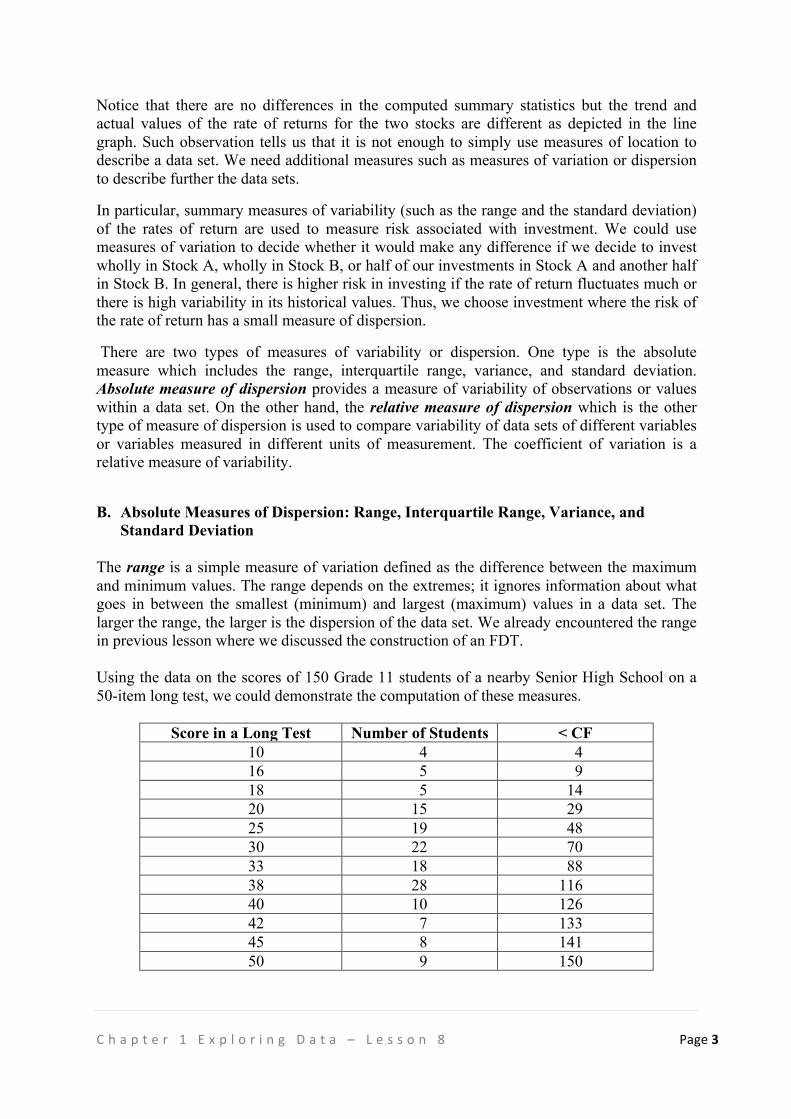
!C h a p t e r ! 1 ! E x p l o r i n g ! D a t a ! – ! L e s s o n ! 8 ! Page!3"! !!!!
Notice that there are no differences in the computed summary statistics but the trend and actual values of the rate of returns for the two stocks are different as depicted in the line graph. Such observation tells us that it is not enough to simply use measures of location to describe a data set. We need additional measures such as measures of variation or dispersion to describe further the data sets.
In particular, summary measures of variability (such as the range and the standard deviation) of the rates of return are used to measure risk associated with investment. We could use measures of variation to decide whether it would make any difference if we decide to invest wholly in Stock A, wholly in Stock B, or half of our investments in Stock A and another half in Stock B. In general, there is higher risk in investing if the rate of return fluctuates much or there is high variability in its historical values. Thus, we choose investment where the risk of the rate of return has a small measure of dispersion.
There are two types of measures of variability or dispersion. One type is the absolute measure which includes the range, interquartile range, variance, and standard deviation. Absolute measure of dispersion provides a measure of variability of observations or values within a data set. On the other hand, the relative measure of dispersion which is the other type of measure of dispersion is used to compare variability of data sets of different variables or variables measured in different units of measurement. The coefficient of variation is a relative measure of variability.
B. Absolute Measures of Dispersion: Range, Interquartile Range, Variance, and Standard Deviation
The range is a simple measure of variation defined as the difference between the maximum and minimum values. The range depends on the extremes; it ignores information about what goes in between the smallest (minimum) and largest (maximum) values in a data set. The larger the range, the larger is the dispersion of the data set. We already encountered the range in previous lesson where we discussed the construction of an FDT. Using the data on the scores of 150 Grade 11 students of a nearby Senior High School on a 50-item long test, we could demonstrate the computation of these measures.
Score in a Long Test Number of Students < CF 10 4 4 16 5 9 18 5 14 20 15 29 25 19 48 30 22 70 33 18 88 38 28 116 40 10 126 42 7 133 45 8 141 50 9 150
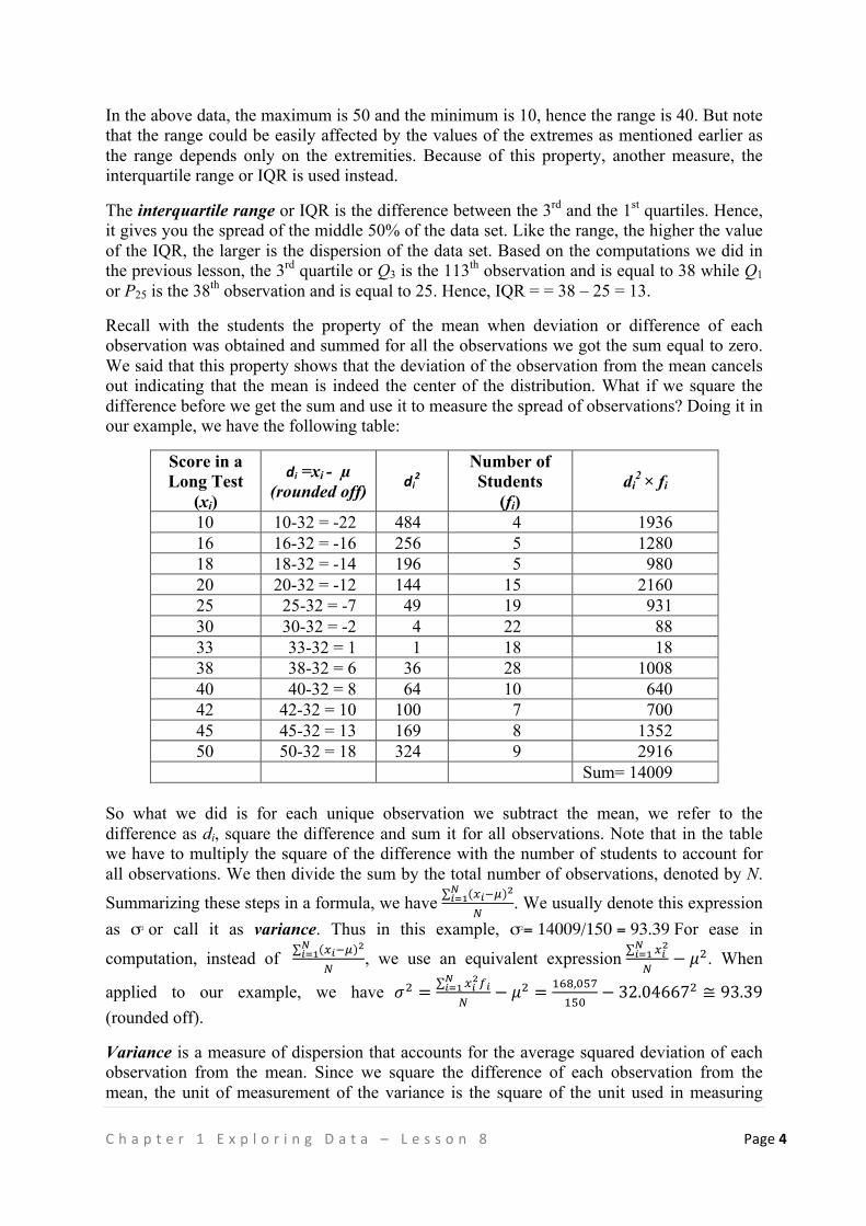
!C h a p t e r ! 1 ! E x p l o r i n g ! D a t a ! – ! L e s s o n ! 8 ! Page!4"! !!!!
In the above data, the maximum is 50 and the minimum is 10, hence the range is 40. But note that the range could be easily affected by the values of the extremes as mentioned earlier as the range depends only on the extremities. Because of this property, another measure, the interquartile range or IQR is used instead.
The interquartile range or IQR is the difference between the 3rd and the 1st quartiles. Hence, it gives you the spread of the middle 50% of the data set. Like the range, the higher the value of the IQR, the larger is the dispersion of the data set. Based on the computations we did in the previous lesson, the 3rd quartile or Q3 is the 113th observation and is equal to 38 while Q1 or P25 is the 38th observation and is equal to 25. Hence, IQR = = 38 – 25 = 13.
Recall with the students the property of the mean when deviation or difference of each observation was obtained and summed for all the observations we got the sum equal to zero. We said that this property shows that the deviation of the observation from the mean cancels out indicating that the mean is indeed the center of the distribution. What if we square the difference before we get the sum and use it to measure the spread of observations? Doing it in our example, we have the following table:
Score in a Long Test
(xi)
di =xi - µ (rounded off) di
2 Number of Students
(fi) di
2 × fi
10 10-32 = -22 484 4 1936 16 16-32 = -16 256 5 1280 18 18-32 = -14 196 5 980 20 20-32 = -12 144 15 2160 25 25-32 = -7 49 19 931 30 30-32 = -2 4 22 88 33 33-32 = 1 1 18 18 38 38-32 = 6 36 28 1008 40 40-32 = 8 64 10 640 42 42-32 = 10 100 7 700 45 45-32 = 13 169 8 1352 50 50-32 = 18 324 9 2916 Sum= 14009
So what we did is for each unique observation we subtract the mean, we refer to the difference as di, square the difference and sum it for all observations. Note that in the table we have to multiply the square of the difference with the number of students to account for all observations. We then divide the sum by the total number of observations, denoted by N.
Summarizing these steps in a formula, we have !!!! !!!!!
! . We usually denote this expression as σ2 or call it as variance. Thus in this example, σ2= 14009/150 = 93.39 For ease in
computation, instead of !!!! !!!!!
! , we use an equivalent expression !!!!!!!! − !!. When
applied to our example, we have !! = !!!!!!!!!! − !! = !"#,!"#
!"# − 32.04667! ≅ 93.39 (rounded off).
Variance is a measure of dispersion that accounts for the average squared deviation of each observation from the mean. Since we square the difference of each observation from the mean, the unit of measurement of the variance is the square of the unit used in measuring
!C h a p t e r ! 1 ! E x p l o r i n g ! D a t a ! – ! L e s s o n ! 8 ! Page!5"! !!!!
each observation. Such property is a little bit problematic in interpretation. For example, point2 or kilogram2 is difficult to interpret compared to inches2.
Hence, instead of the variance the standard deviation is computed which is the positive square of the variance, that is, ! = !!. In the example,!! = 93.3933 = 9.6640. To interpret, we say that on the average, the scores of the students deviate from the mean score of 32 points by as much as 9.6640 or approximately 10 points.
If all the observations are equal to a constant, then the mean is that constant, and the measure of variation is zero. Furthermore, if for a given data set, the variance and standard deviation turn out to be zero, then all the deviations from the average must be zero, which means that all observations are equal. Note that if a data set were rescaled, that is if the observations were multiplied by some constant, then the standard deviation of the new data set is merely the scaling factor multiplied to the standard deviation of the original data set. The variance and standard deviation are based on all the observations items in the data set, and each item is given a proper weight. They are extremely useful measures of variability as they measure the average scattering of the data around the mean, that is how large data fluctuate above and below the mean. The variance and standard deviation increase with an increase in the deviations about the mean, and decrease with decreases in these deviations. A small standard deviation (and variance) means a high degree of uniformity in the observations and of homogeneity in a series. The variance is the most suitable for algebraic manipulations but as was pointed out earlier, its value is in squared unit of measurements. On the other hand, the standard deviation has unit of measure same as with that of the observations. Thus, standard deviation serves as the primary measure of variation, just as the mean is the primary measure of central location. Going back to the motivation example on the stocks where in we have two stocks, A and B. Both stocks have same expected return measured by the mean. However, the standard deviation of the rates of return for Stock A is 0.0688 while that for Stock B is 0.0685, indicating that Stock A has higher risk compared to Stock B although the difference is not that large. C. Relative Measure of Dispersion: Coefficient of Variation To compare variability between or among different data sets, that is, the data sets are for different variables or same variables but measured in different unit of measurement, the coefficient of variation (CV) is used as measure of relative dispersion. It is usually expressed as percentage and is computed as CV = !
!×100%. CV is a measure of dispersion relative to the mean of the data set. With and having same unit of measurement, CV is unit less or it does not depend on the unit of measurement. Hence, it is used compare the variability across the different data sets. As an example, the CV of the scores of the students in the long test is computed as CV = !
!×100% = ! !.!!"#!".!"##$×100% = 30.16% while the CV of the rate of returns of Stock A
is CV = !.!"##!.!"#$×100% = 42.34%. Thus, we say the rate of returns of Stock A is more
!C h a p t e r ! 1 ! E x p l o r i n g ! D a t a ! – ! L e s s o n ! 8 ! Page!6"! !!!!
variable than the scores of the students in the test. Here, we used the CV to compare the variability of two different data sets. KEY POINTS • Measure of dispersion is used to further describe the distribution of the data set. • Absolute measures of variation include range, interquartile range, variance and standard
deviation. • A relative measure of dispersion is provided by the coefficient of variation.
REFERENCES Albert, J. R. G. (2008). Basic Statistics for the Tertiary Level (ed. Roberto Padua, WelfredoPatungan, Nelia Marquez), published by Rex Bookstore.
Bryant−Smith (2009): Practical Data Analysis, Second Edition. McGraw-Hill/Irvine, USA.
Handbook of Statistics 1 (1st and 2nd Edition), Authored by the Faculty of the Institute of Statistics, UP Los Baños, College Laguna 4031
Moore, D.S. (2007). The Basic Practice of Statistics, Fourth Edition W.H. Freeman and Company.
“Range as a Measure of Variation” http://www.sharemylesson.com/teaching-resource/range-as-a-measure-of-variation-50009362
Workbooks in Statistics 1 (From 1st to 13th Edition), Authored by the Faculty of the Institute of Statistics, UP Los Baños, College Laguna 4031
!C h a p t e r ! 1 ! E x p l o r i n g ! D a t a ! – ! L e s s o n ! 8 ! Page!7"! !!!!
ASSESSMENT Note: Answers are provided inside the parentheses and in bold face. 1. Three friends, Gerald, Carmina, and Rodolfo are planning their business of selling homemade peanut butter. They start the planning by doing a market study where they obtained the prices (in pesos) of a 250-gram jar of several known brands of peanut butter. Below is the data set they have collected:
100.80 197.60 158.00 131.60 184.40 149.20 136.00 109.60 360.40 122.80 131.60
After studying the data, Gerald said, “The prices of peanut butter are pretty similar. The range is only PhP 30.80.” Carmina said, “You are mistaken! The prices are very different. The range is PhP 259.60. Rodolfo said, “I think you are both mistaken. The range isn’t a useful measure to describe the variation of the data set. a. Explain what you think is the basis used by each person in support of their claims. (Gerald did not arrange the data set from smallest to largest, and erroneously subtracted the first value (100.80) from the last value (131.60) in the data set. Carmina found the range correctly by subtracting the smallest value (100.80) from the largest value (360.40). Rodolfo noticed that the maximum 360.80 is an outlier. As a result, the computed range of PhP259.60 roughly describe the variation of the observations as it was unduly increased by the extreme value.) b. Who should we agree with? Why? (We can agree with both Carmina and Rodolfo. Carmina correctly calculated the range; Rodolfo intelligently observed that while Carmina was correct in her calculation, the range is not very useful in describing the variability of the observations, as the range would only be PHP 96.80 if the outlier were removed from the data set.) 2. Three hundred students taking a basic course in Statistics are given similar final examination. After checking the papers and while the professor is studying the distribution of the final examination scores, he taught of several scenarios which are described below: a. Suppose the professor will give 30% weight to the final examination, what effect would multiplying 30% on all the final scores have on the mean of the final exam scores? On the standard deviation of the final exam scores? (The mean will also get rescaled by 30%, so with the standard deviation.)
b. Suppose the professor wants to bloat the final examination scores, what will be the effect to the mean of the final exam scores if 5 points will be added to each of the final score? On the standard deviation of the final exam scores? (The mean will also go up by 5 points; while standard deviation stays the same.) 3. In a fitness center, weights of a certain group of students were taken resulting to a common weight of 140 pounds. What would be the standard deviation of the distribution of weights? (Zero, since the observations do not vary.)
!C h a p t e r ! 1 ! E x p l o r i n g ! D a t a ! – ! L e s s o n ! 8 ! Page!8"! !!!!
4. Determine which of the following statements is (are) TRUE or FALSE. Explain briefly your answer. a. If each observation in a data set is doubled, then the standard deviation would also be
doubled. (True, since the variance would be quadrupled and taking the square root of the resulting variance, will result to twice the standard deviation.)
b. If in a set of data, positive numbers are changed to negative, while negative are
changed to positive, then the standard deviation changes its sign as well. (False, since standard deviation is always nonnegative.)
Explanatory Note:
Teachers have the option to ask this assessment orally to the entire class to either introduce or recall the notions of computing the range and of computing the standard deviation, or to group students and ask them to identify answers, or to give this as homework, or to use some questions/items here for a chapter examination.
C h a p t e r ( 1 ( E x p l o r i n g ( D a t a ( – ( L e s s o n ( 9 ( Page(1"((
Chapter 1: Exploring Data Lesson 9: More on Describing Data: SummaryMeasures and
Graphs
TIME FRAME:1 hour session
OVERVIEW OF LESSON: In this lesson, students will do an activity that will use the data on heights and weights which were collected in Lesson 2. They will construct box plots and calculate the summary measures they have learned in previous lessons. These computed summary measures and constructed boxplot will be used to describe fully the data set so as to provide simple analysis of the data at hand.
LEARNING OUTCOME(S): At the end of the lesson, the learner is able to • Construct and interpret box plots; and • Provide simple analysis of a data set based on its descriptive measures.
LESSON OUTLINE: 1. Preliminaries: Teacher’s Preparation for the Lesson 2. Motivation: The Student’s Height and Weight and Corresponding BMI 3. Construction and Interpretation of a Box-plot
DEVELOPMENT OF THE LESSON
A. Preliminaries: Teacher’s Preparation for the Lesson Note: This is an activity that the teacher has to do in preparation for the lesson.
A day before the actual schedule for this lesson, you should review some information about the body mass index (BMI) so that you could compute the BMI of each student in the class based on the students’ weights and heights collected in Lesson 2. This will also make you more confident to discuss BMI in the class as well as use it to integrate the lessons learned in this chapter. The following discussion provides useful information about BMI.
The BMI, devised by Adolphe Quetelet, is defined as the body mass divided by the square of the body height, and is universally expressed in units of kg/m2, using weight in kilograms and height in meters. When the term BMI is used informally, the units are usually omitted. A high BMI can be an indicator of high body fatness. The BMI can be used to screen for weight categories that may lead to health problems.
The BMI provides a simple numeric measure of a person's thickness or thinness, allowing medical and health professionals to discuss weight problems more objectively with the adult
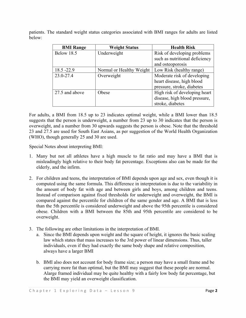
C h a p t e r ( 1 ( E x p l o r i n g ( D a t a ( – ( L e s s o n ( 9 ( Page(2"((
patients. The standard weight status categories associated with BMI ranges for adults are listed below:
BMI Range Weight Status Health Risk Below 18.5 Underweight Risk of developing problems
such as nutritional deficiency and osteoporosis
18.5 -22.9 Normal or Healthy Weight Low Risk (healthy range) 23.0-27.4 Overweight Moderate risk of developing
heart disease, high blood pressure, stroke, diabetes
27.5 and above Obese High risk of developing heart disease, high blood pressure, stroke, diabetes
For adults, a BMI from 18.5 up to 23 indicates optimal weight, while a BMI lower than 18.5 suggests that the person is underweight, a number from 23 up to 30 indicates that the person is overweight, and a number from 30 upwards suggests the person is obese. Note that the threshold 23 and 27.5 are used for South East Asians, as per suggestion of the World Health Organization (WHO), though generally 25 and 30 are used.
Special Notes about interpreting BMI:
1. Many but not all athletes have a high muscle to fat ratio and may have a BMI that is misleadingly high relative to their body fat percentage. Exceptions also can be made for the elderly, and the infirm.
2. For children and teens, the interpretation of BMI depends upon age and sex, even though it is
computed using the same formula. This difference in interpretation is due to the variability in the amount of body fat with age and between girls and boys, among children and teens. Instead of comparison against fixed thresholds for underweight and overweight, the BMI is compared against the percentile for children of the same gender and age. A BMI that is less than the 5th percentile is considered underweight and above the 95th percentile is considered obese. Children with a BMI between the 85th and 95th percentile are considered to be overweight.
3. The following are other limitations in the interpretation of BMI.
a. Since the BMI depends upon weight and the square of height, it ignores the basic scaling law which states that mass increases to the 3rd power of linear dimensions. Thus, taller individuals, even if they had exactly the same body shape and relative composition, always have a larger BMI
b. BMI also does not account for body frame size; a person may have a small frame and be carrying more fat than optimal, but the BMI may suggest that these people are normal. Alarge framed individual may be quite healthy with a fairly low body fat percentage, but the BMI may yield an overweight classification.
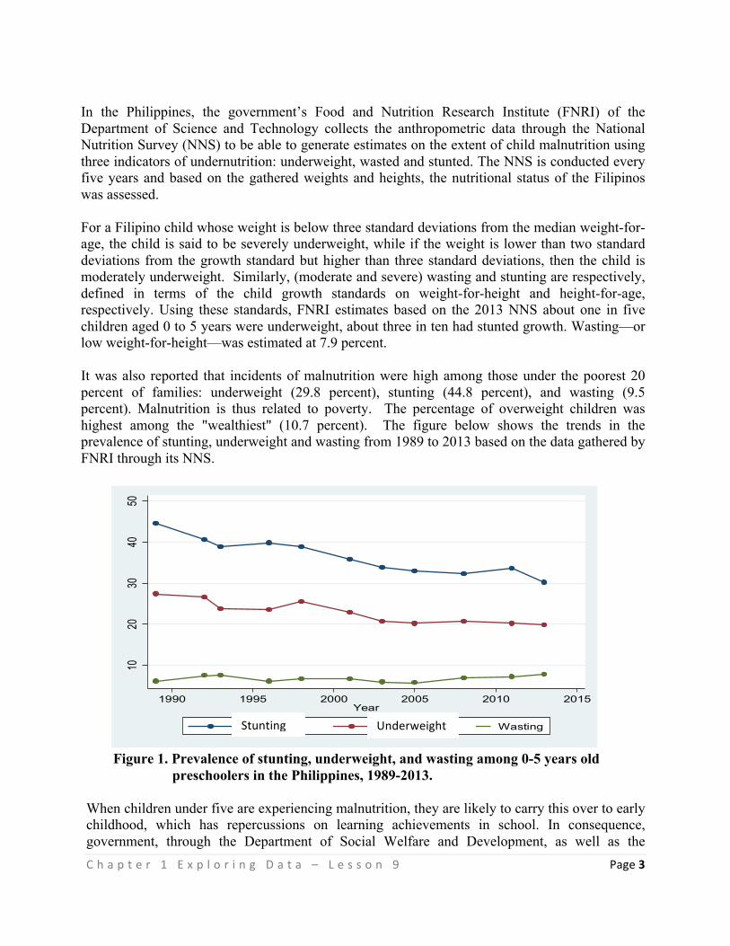
C h a p t e r ( 1 ( E x p l o r i n g ( D a t a ( – ( L e s s o n ( 9 ( Page(3"((
In the Philippines, the government’s Food and Nutrition Research Institute (FNRI) of the Department of Science and Technology collects the anthropometric data through the National Nutrition Survey (NNS) to be able to generate estimates on the extent of child malnutrition using three indicators of undernutrition: underweight, wasted and stunted. The NNS is conducted every five years and based on the gathered weights and heights, the nutritional status of the Filipinos was assessed. For a Filipino child whose weight is below three standard deviations from the median weight-for-age, the child is said to be severely underweight, while if the weight is lower than two standard deviations from the growth standard but higher than three standard deviations, then the child is moderately underweight. Similarly, (moderate and severe) wasting and stunting are respectively, defined in terms of the child growth standards on weight-for-height and height-for-age, respectively. Using these standards, FNRI estimates based on the 2013 NNS about one in five children aged 0 to 5 years were underweight, about three in ten had stunted growth. Wasting—or low weight-for-height—was estimated at 7.9 percent. It was also reported that incidents of malnutrition were high among those under the poorest 20 percent of families: underweight (29.8 percent), stunting (44.8 percent), and wasting (9.5 percent). Malnutrition is thus related to poverty. The percentage of overweight children was highest among the "wealthiest" (10.7 percent). The figure below shows the trends in the prevalence of stunting, underweight and wasting from 1989 to 2013 based on the data gathered by FNRI through its NNS.
Figure 1. Prevalence of stunting, underweight, and wasting among 0-5 years old
preschoolers in the Philippines, 1989-2013.
When children under five are experiencing malnutrition, they are likely to carry this over to early childhood, which has repercussions on learning achievements in school. In consequence, government, through the Department of Social Welfare and Development, as well as the
1020
3040
50
1990 1995 2000 2005 2010 2015Year
Underweight Stunting Wasting (Stunting( Underweight(
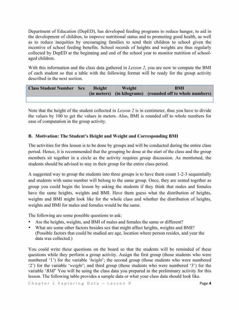
C h a p t e r ( 1 ( E x p l o r i n g ( D a t a ( – ( L e s s o n ( 9 ( Page(4"((
Department of Education (DepED), has developed feeding programs to reduce hunger, to aid in the development of children, to improve nutritional status and to promoting good health, as well as to reduce inequities by encouraging families to send their children to school given the incentive of school feeding benefits. School records of heights and weights are thus regularly collected by DepED at the beginning and end of the school year to monitor nutrition of school-aged children.
With this information and the class data gathered in Lesson 2, you are now to compute the BMI of each student so that a table with the following format will be ready for the group activity described in the next section.
Class Student Number Sex Height (in meters)
Weight (in kilograms)
BMI (rounded off to whole numbers)
Note that the height of the student collected in Lesson 2 is in centimeter, thus you have to divide the values by 100 to get the values in meters. Also, BMI is rounded off to whole numbers for ease of computation in the group activity.
B. Motivation: The Student’s Height and Weight and Corresponding BMI
The activities for this lesson is to be done by groups and will be conducted during the entire class period. Hence, it is recommended that the grouping be done at the start of the class and the group members sit together in a circle as the activity requires group discussion. As mentioned, the students should be advised to stay in their group for the entire class period.
A suggested way to group the students into three groups is to have them count 1-2-3 sequentially and students with same number will belong to the same group. Once, they are seated together as group you could begin the lesson by asking the students if they think that males and females have the same heights, weights and BMI. Have them guess what the distribution of heights, weights and BMI might look like for the whole class and whether the distribution of heights, weights and BMI for males and females would be the same.
The following are some possible questions to ask: • Are the heights, weights, and BMI of males and females the same or different? • What are some other factors besides sex that might affect heights, weights and BMI?
(Possible factors that could be studied are age, location where person resides, and year the data was collected.)
You could write these questions on the board so that the students will be reminded of these questions while they perform a group activity. Assign the first group (those students who were numbered ‘1’) for the variable ‘height’; the second group (those students who were numbered ‘2’) for the variable ‘weight’; and third group (those students who were numbered ‘3’) for the variable ‘BMI’ You will be using the class data you prepared in the preliminary activity for this lesson. The following table provides a sample data or what your class data should look like.
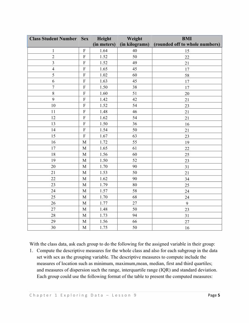
C h a p t e r ( 1 ( E x p l o r i n g ( D a t a ( – ( L e s s o n ( 9 ( Page(5"((
Class Student Number Sex Height
(in meters) Weight
(in kilograms) BMI
(rounded off to whole numbers) 1 F 1.64 40 15 2 F 1.52 50 22 3 F 1.52 49 21 4 F 1.65 45 17 5 F 1.02 60 58 6 F 1.63 45 17 7 F 1.50 38 17 8 F 1.60 51 20 9 F 1.42 42 21
10 F 1.52 54 23 11 F 1.48 46 21 12 F 1.62 54 21 13 F 1.50 36 16 14 F 1.54 50 21 15 F 1.67 63 23 16 M 1.72 55 19 17 M 1.65 61 22 18 M 1.56 60 25 19 M 1.50 52 23 20 M 1.70 90 31 21 M 1.53 50 21 22 M 1.62 90 34 23 M 1.79 80 25 24 M 1.57 58 24 25 M 1.70 68 24 26 M 1.77 27 9 27 M 1.48 50 23 28 M 1.73 94 31 29 M 1.56 66 27 30 M 1.75 50 16
With the class data, ask each group to do the following for the assigned variable in their group: 1. Compute the descriptive measures for the whole class and also for each subgroup in the data
set with sex as the grouping variable. The descriptive measures to compute include the measures of location such as minimum, maximum,mean, median, first and third quartiles; and measures of dispersion such the range, interquartile range (IQR) and standard deviation. Each group could use the following format of the table to present the computed measures:
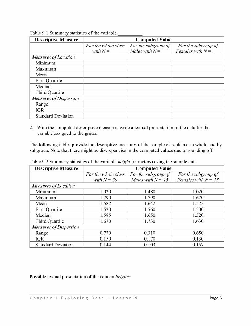
C h a p t e r ( 1 ( E x p l o r i n g ( D a t a ( – ( L e s s o n ( 9 ( Page(6"((
Table 9.1 Summary statistics of the variable __________. Descriptive Measure Computed Value
For the whole class with N = ___
For the subgroup of Males with N = ___
For the subgroup of Females with N = ___
Measures of Location Minimum Maximum Mean First Quartile Median Third Quartile Measures of Dispersion Range IQR Standard Deviation
2. With the computed descriptive measures, write a textual presentation of the data for the
variable assigned to the group. The following tables provide the descriptive measures of the sample class data as a whole and by subgroup. Note that there might be discrepancies in the computed values due to rounding off. Table 9.2 Summary statistics of the variable height (in meters) using the sample data.
Descriptive Measure Computed Value For the whole class
with N = 30 For the subgroup of Males with N = 15
For the subgroup of Females with N = 15
Measures of Location Minimum 1.020 1.480 1.020 Maximum 1.790 1.790 1.670 Mean 1.582 1.642 1.522 First Quartile 1.520 1.560 1.500 Median 1.585 1.650 1.520 Third Quartile 1.670 1.730 1.630 Measures of Dispersion Range 0.770 0.310 0.650 IQR 0.150 0.170 0.130 Standard Deviation 0.144 0.103 0.157
Possible textual presentation of the data on heights:
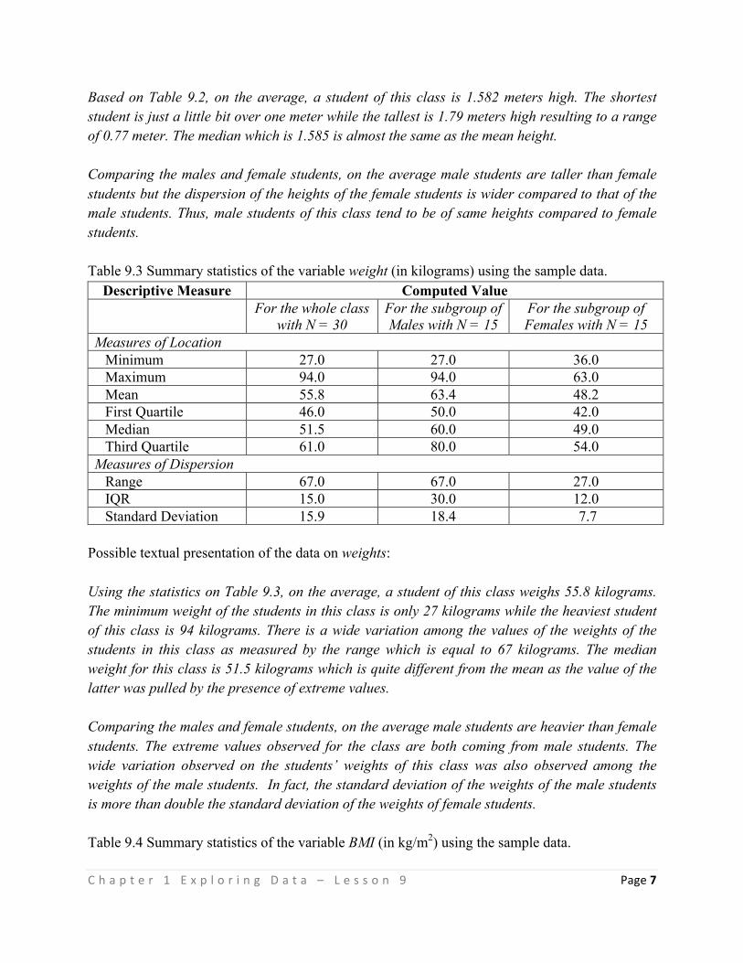
C h a p t e r ( 1 ( E x p l o r i n g ( D a t a ( – ( L e s s o n ( 9 ( Page(7"((
Based on Table 9.2, on the average, a student of this class is 1.582 meters high. The shortest student is just a little bit over one meter while the tallest is 1.79 meters high resulting to a range of 0.77 meter. The median which is 1.585 is almost the same as the mean height. Comparing the males and female students, on the average male students are taller than female students but the dispersion of the heights of the female students is wider compared to that of the male students. Thus, male students of this class tend to be of same heights compared to female students. Table 9.3 Summary statistics of the variable weight (in kilograms) using the sample data.
Descriptive Measure Computed Value For the whole class
with N = 30 For the subgroup of Males with N = 15
For the subgroup of Females with N = 15
Measures of Location Minimum 27.0 27.0 36.0 Maximum 94.0 94.0 63.0 Mean 55.8 63.4 48.2 First Quartile 46.0 50.0 42.0 Median 51.5 60.0 49.0 Third Quartile 61.0 80.0 54.0 Measures of Dispersion Range 67.0 67.0 27.0 IQR 15.0 30.0 12.0 Standard Deviation 15.9 18.4 7.7
Possible textual presentation of the data on weights: Using the statistics on Table 9.3, on the average, a student of this class weighs 55.8 kilograms. The minimum weight of the students in this class is only 27 kilograms while the heaviest student of this class is 94 kilograms. There is a wide variation among the values of the weights of the students in this class as measured by the range which is equal to 67 kilograms. The median weight for this class is 51.5 kilograms which is quite different from the mean as the value of the latter was pulled by the presence of extreme values. Comparing the males and female students, on the average male students are heavier than female students. The extreme values observed for the class are both coming from male students. The wide variation observed on the students’ weights of this class was also observed among the weights of the male students. In fact, the standard deviation of the weights of the male students is more than double the standard deviation of the weights of female students. Table 9.4 Summary statistics of the variable BMI (in kg/m2) using the sample data.
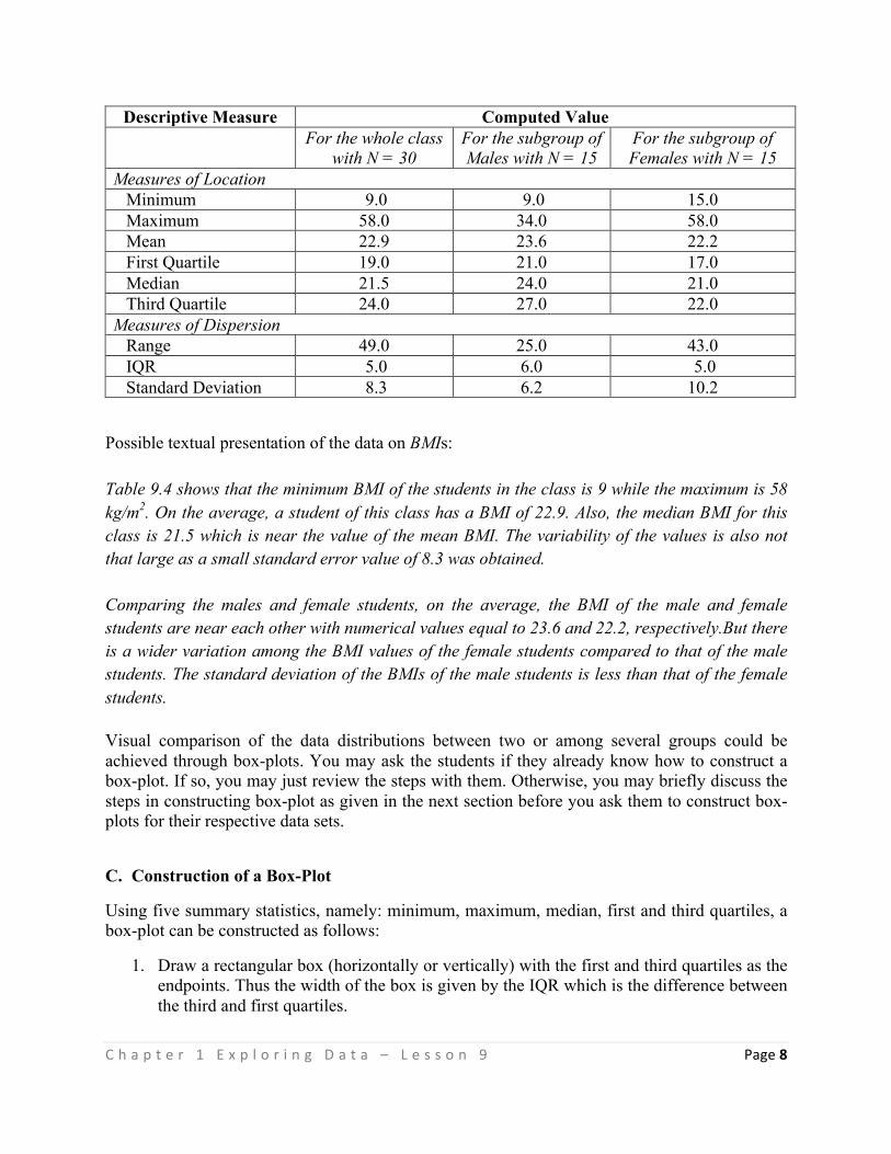
C h a p t e r ( 1 ( E x p l o r i n g ( D a t a ( – ( L e s s o n ( 9 ( Page(8"((
Descriptive Measure Computed Value For the whole class
with N = 30 For the subgroup of Males with N = 15
For the subgroup of Females with N = 15
Measures of Location Minimum 9.0 9.0 15.0 Maximum 58.0 34.0 58.0 Mean 22.9 23.6 22.2 First Quartile 19.0 21.0 17.0 Median 21.5 24.0 21.0 Third Quartile 24.0 27.0 22.0 Measures of Dispersion Range 49.0 25.0 43.0 IQR 5.0 6.0 5.0 Standard Deviation 8.3 6.2 10.2
Possible textual presentation of the data on BMIs: Table 9.4 shows that the minimum BMI of the students in the class is 9 while the maximum is 58 kg/m2. On the average, a student of this class has a BMI of 22.9. Also, the median BMI for this class is 21.5 which is near the value of the mean BMI. The variability of the values is also not that large as a small standard error value of 8.3 was obtained. Comparing the males and female students, on the average, the BMI of the male and female students are near each other with numerical values equal to 23.6 and 22.2, respectively.But there is a wider variation among the BMI values of the female students compared to that of the male students. The standard deviation of the BMIs of the male students is less than that of the female students. Visual comparison of the data distributions between two or among several groups could be achieved through box-plots. You may ask the students if they already know how to construct a box-plot. If so, you may just review the steps with them. Otherwise, you may briefly discuss the steps in constructing box-plot as given in the next section before you ask them to construct box-plots for their respective data sets.
C. Construction of a Box-Plot
Using five summary statistics, namely: minimum, maximum, median, first and third quartiles, a box-plot can be constructed as follows:
1. Draw a rectangular box (horizontally or vertically) with the first and third quartiles as the endpoints. Thus the width of the box is given by the IQR which is the difference between the third and first quartiles.
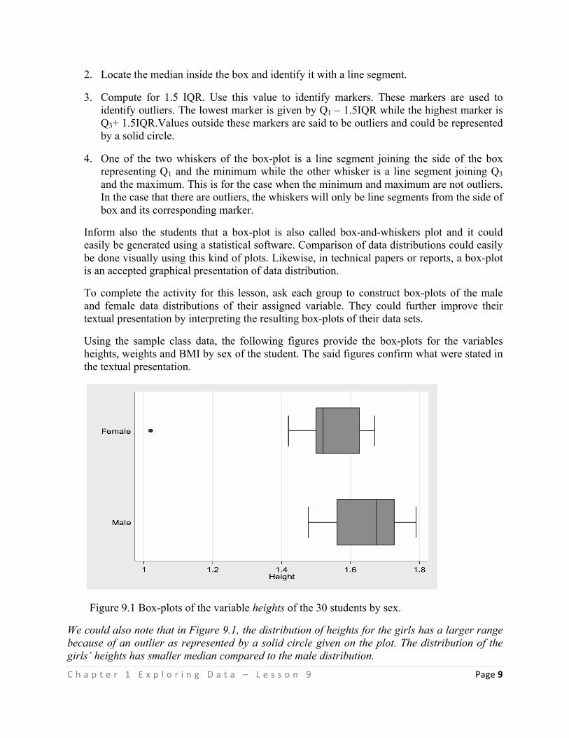
C h a p t e r ( 1 ( E x p l o r i n g ( D a t a ( – ( L e s s o n ( 9 ( Page(9"((
2. Locate the median inside the box and identify it with a line segment.
3. Compute for 1.5 IQR. Use this value to identify markers. These markers are used to identify outliers. The lowest marker is given by Q1 – 1.5IQR while the highest marker is Q3+ 1.5IQR.Values outside these markers are said to be outliers and could be represented by a solid circle.
4. One of the two whiskers of the box-plot is a line segment joining the side of the box representing Q1 and the minimum while the other whisker is a line segment joining Q3 and the maximum. This is for the case when the minimum and maximum are not outliers. In the case that there are outliers, the whiskers will only be line segments from the side of box and its corresponding marker.
Inform also the students that a box-plot is also called box-and-whiskers plot and it could easily be generated using a statistical software. Comparison of data distributions could easily be done visually using this kind of plots. Likewise, in technical papers or reports, a box-plot is an accepted graphical presentation of data distribution.
To complete the activity for this lesson, ask each group to construct box-plots of the male and female data distributions of their assigned variable. They could further improve their textual presentation by interpreting the resulting box-plots of their data sets.
Using the sample class data, the following figures provide the box-plots for the variables heights, weights and BMI by sex of the student. The said figures confirm what were stated in the textual presentation.
Figure 9.1 Box-plots of the variable heights of the 30 students by sex.
We could also note that in Figure 9.1, the distribution of heights for the girls has a larger range because of an outlier as represented by a solid circle given on the plot. The distribution of the girls’ heights has smaller median compared to the male distribution.
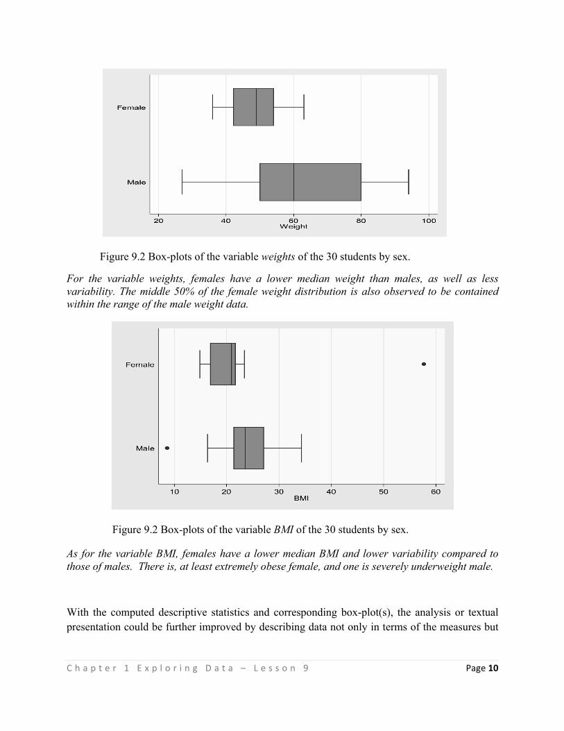
C h a p t e r ( 1 ( E x p l o r i n g ( D a t a ( – ( L e s s o n ( 9 ( Page(10"((
Figure 9.2 Box-plots of the variable weights of the 30 students by sex.
For the variable weights, females have a lower median weight than males, as well as less variability. The middle 50% of the female weight distribution is also observed to be contained within the range of the male weight data.
Figure 9.2 Box-plots of the variable BMI of the 30 students by sex.
As for the variable BMI, females have a lower median BMI and lower variability compared to those of males. There is, at least extremely obese female, and one is severely underweight male.
With the computed descriptive statistics and corresponding box-plot(s), the analysis or textual presentation could be further improved by describing data not only in terms of the measures but
C h a p t e r ( 1 ( E x p l o r i n g ( D a t a ( – ( L e s s o n ( 9 ( Page(11"((
also in terms of the interpretation of box plots. Furthermore, these measures allow us to answer the guide questions provided at the start of the class.
KEY POINTS
• Descriptive measures are important statistics required in simple data analysis. • Groups of data could be compared in terms of their descriptive measures. • A box-plot is an approach to compare visually data distributions.
REFERENCES
Albert, J. R. G. (2008). Basic Statistics for the Tertiary Level (ed. Roberto Padua, WelfredoPatungan, Nelia Marquez), published by Rex Bookstore.
“Armspans” inSTatistics Education Web (STEW) http://www.amstat.org/education/stew/pdfs/Armspans.docx “Deciding Which Measure of Center to Use” http://www.sharemylesson.com/teaching-resource/deciding-which-measure-of-center-to-use-50013703/
Handbook of Statistics 1 (1st and 2nd Edition), Authored by the Faculty of the Institute of Statistics, UP Los Baños, College Laguna 4031
Workbooks in Statistics 1 (From 1st to 13th Edition), Authored by the Faculty of the Institute of Statistics, UP Los Baños, College Laguna 4031
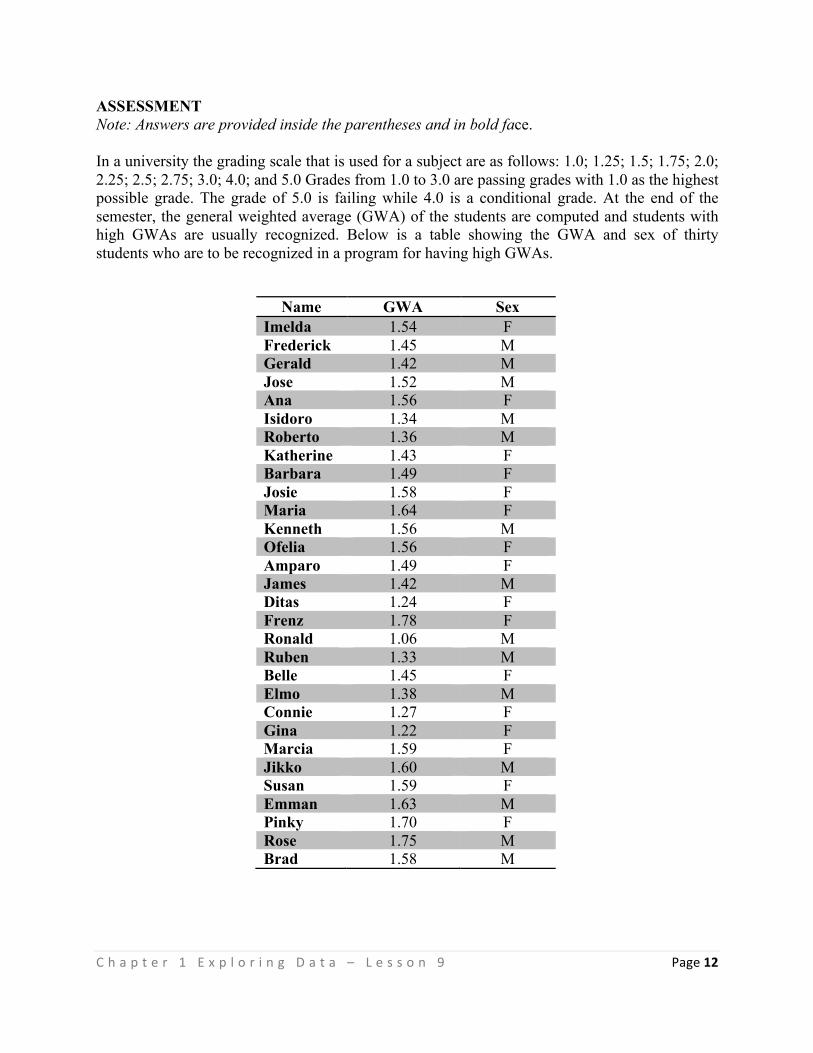
C h a p t e r ( 1 ( E x p l o r i n g ( D a t a ( – ( L e s s o n ( 9 ( Page(12"((
ASSESSMENT Note: Answers are provided inside the parentheses and in bold face. In a university the grading scale that is used for a subject are as follows: 1.0; 1.25; 1.5; 1.75; 2.0; 2.25; 2.5; 2.75; 3.0; 4.0; and 5.0 Grades from 1.0 to 3.0 are passing grades with 1.0 as the highest possible grade. The grade of 5.0 is failing while 4.0 is a conditional grade. At the end of the semester, the general weighted average (GWA) of the students are computed and students with high GWAs are usually recognized. Below is a table showing the GWA and sex of thirty students who are to be recognized in a program for having high GWAs.
Name GWA Sex
Imelda 1.54 F Frederick 1.45 M Gerald 1.42 M Jose 1.52 M Ana 1.56 F Isidoro 1.34 M Roberto 1.36 M Katherine 1.43 F Barbara 1.49 F Josie 1.58 F Maria 1.64 F Kenneth 1.56 M Ofelia 1.56 F Amparo 1.49 F James 1.42 M Ditas 1.24 F Frenz 1.78 F Ronald 1.06 M Ruben 1.33 M Belle 1.45 F Elmo 1.38 M Connie 1.27 F Gina 1.22 F Marcia 1.59 F Jikko 1.60 M Susan 1.59 F Emman 1.63 M Pinky 1.70 F Rose 1.75 M Brad 1.58 M
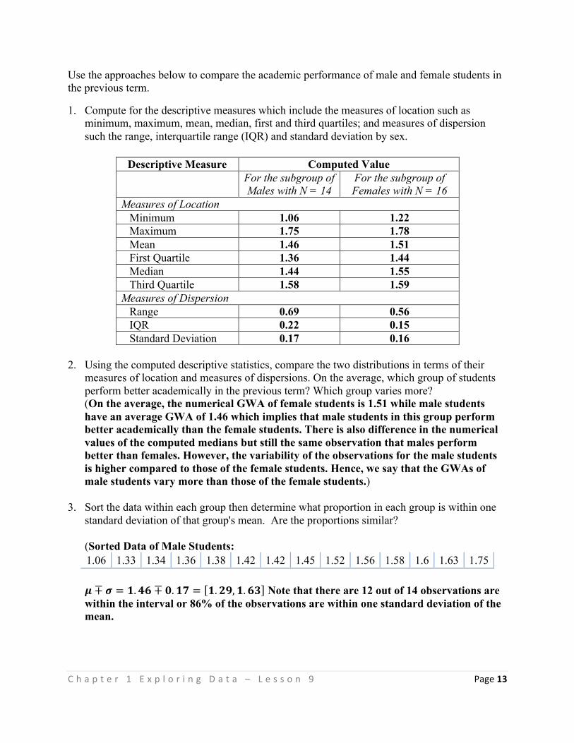
C h a p t e r ( 1 ( E x p l o r i n g ( D a t a ( – ( L e s s o n ( 9 ( Page(13"((
Use the approaches below to compare the academic performance of male and female students in the previous term.
1. Compute for the descriptive measures which include the measures of location such as minimum, maximum, mean, median, first and third quartiles; and measures of dispersion such the range, interquartile range (IQR) and standard deviation by sex.
Descriptive Measure Computed Value For the subgroup of
Males with N = 14 For the subgroup of Females with N = 16
Measures of Location Minimum 1.06 1.22 Maximum 1.75 1.78 Mean 1.46 1.51 First Quartile 1.36 1.44 Median 1.44 1.55 Third Quartile 1.58 1.59 Measures of Dispersion Range 0.69 0.56 IQR 0.22 0.15 Standard Deviation 0.17 0.16
2. Using the computed descriptive statistics, compare the two distributions in terms of their
measures of location and measures of dispersions. On the average, which group of students perform better academically in the previous term? Which group varies more? (On the average, the numerical GWA of female students is 1.51 while male students have an average GWA of 1.46 which implies that male students in this group perform better academically than the female students. There is also difference in the numerical values of the computed medians but still the same observation that males perform better than females. However, the variability of the observations for the male students is higher compared to those of the female students. Hence, we say that the GWAs of male students vary more than those of the female students.)
3. Sort the data within each group then determine what proportion in each group is within one standard deviation of that group's mean. Are the proportions similar? (Sorted Data of Male Students: 1.06 1.33 1.34 1.36 1.38 1.42 1.42 1.45 1.52 1.56 1.58 1.6 1.63 1.75 !∓ ! = !.!"∓ !.!" = !.!",!.!" Note that there are 12 out of 14 observations are within the interval or 86% of the observations are within one standard deviation of the mean.
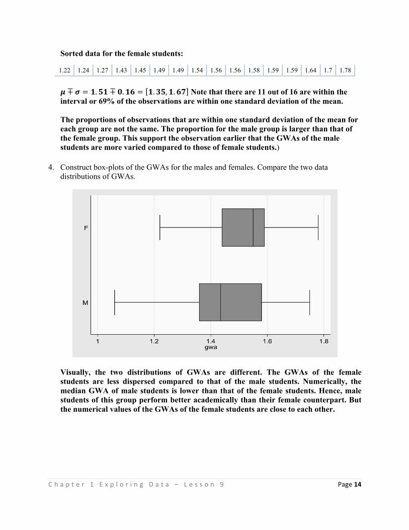
C h a p t e r ( 1 ( E x p l o r i n g ( D a t a ( – ( L e s s o n ( 9 ( Page(14"((
Sorted data for the female students:
1.22 1.24 1.27 1.43 1.45 1.49 1.49 1.54 1.56 1.56 1.58 1.59 1.59 1.64 1.7 1.78
!∓ ! = !.!"∓ !.!" = !.!",!.!" Note that there are 11 out of 16 are within the interval or 69% of the observations are within one standard deviation of the mean. The proportions of observations that are within one standard deviation of the mean for each group are not the same. The proportion for the male group is larger than that of the female group. This support the observation earlier that the GWAs of the male students are more varied compared to those of female students.)
4. Construct box-plots of the GWAs for the males and females. Compare the two data distributions of GWAs.
Visually, the two distributions of GWAs are different. The GWAs of the female students are less dispersed compared to that of the male students. Numerically, the median GWA of male students is lower than that of the female students. Hence, male students of this group perform better academically than their female counterpart. But the numerical values of the GWAs of the female students are close to each other.