engg2450 probability and statistics for...

ENGG2450 Probability and Statistics for EngineersENGG2450 Probability and Statistics for Engineers1 Introduction3 Probabilityy4 Probability distributions5 Probability Densities5 Probability Densities2 Organization and description of data6 Sampling distributions6 Sampling distributions7 Inferences concerning a mean

C8 Comparing two treatments9 Inferences concerning variancesA Random Processes

7 Inferences concerning a mean

7.1 Point estimation

1 Introduction3 Probability4 Probability distributions5 Probability densities2 Organization & description

7.2 Interval estimation2 Organization & description6 Sampling distributions7 Inferences .. mean8 Comparing 2 treatments9 Inferences .. variancesA Random processes

7.4 Tests of hypotheses

7 5 Null hypotheses and tests of

A Random processes

7.5 Null hypotheses and tests of hypotheses

7.6 Hypotheses concerning one mean

7 7 The relation between tests and7.7 The relation between tests and confidence intervals

7.4 Tests of hypotheses (3)

Th bl t d id h th t t tThere are many problems we must decide whether a statement concerning a parameter is true or false; that is, we must test a hypothesis about a parameter.

e.g. Consider the problem of monitoring the quality of water leaving a plant Why does evaluating a sample of specimens not

yp p

leaving a plant. Why does evaluating a sample of specimens not always lead to correct conclusions regarding water quality?

sln. The observed values of water quality depends on the particular specimens in the sample. These values vary from sample to sample Some samples can produce misleadingsample to sample. Some samples can produce misleading values and hence incorrect decisions.

The possibility of making a mistake about water quality, on the basis of test specimens, cannot be completely eliminated nless all ater co ld be acc ratel meas red for the entireunless all water could be accurately measured for the entire

report period.

Suppose that a consumer protection agency wants to test a paint manufacturer’s claim that the average drying time of its new “fast-drying” paint is 20 minutes The agency instructs a research assistant to paint eachpaint is 20 minutes. The agency instructs a research assistant to paint each of 36 boards using a different 1-gallon can of the paint.If the mean of the drying times exceeds 20.75 minutes, then the claim is rejected. If not, the claim is accepted.

This procedure is clear-cut but not infallible. There is a possibility that the sample mean exceeds 20.75 minutes even though the true mean drying time (i.e. population mean ) is 20 minutes.

0-XZThus, we need to know what is that probability.

Assume (1) it is known from past n0Z

That probabilityis

experience that =2.4 minutes, (2) the population is infinite.

is0.0304

=20 20.75

4.0364.2

nx

X

Accept the claimthat =20

Reject the claimthat =20

875.14.0

2075.20

nxz

-

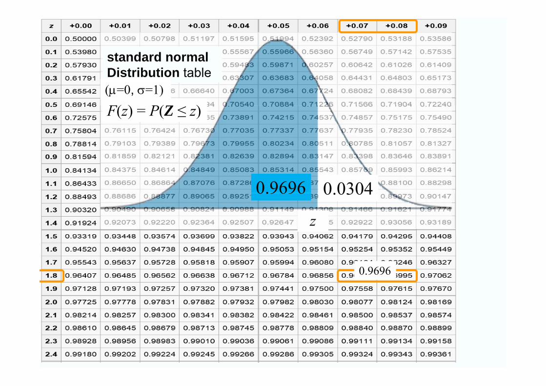
standard normal Distribution table(=0, =1)

F( ) P(Z )F(z) = P(Z ≤ z)

0.9696 0.0304

z

0.9696 0.0304

0.9696

continued: Suppose that a consumer protection agency wants to test a paint manufacturer’s claim that the average drying time of its new “fast-drying” paint is 20minutes. The agency instructs a research assistant to paint each of 36 boards usingminutes. The agency instructs a research assistant to paint each of 36 boards using a different 1-gallon can of the paint. If the mean of the drying times exceeds 20.75minutes, then the claim is rejected. If not, the claim is accepted.

Also, there is a possibility that the sample mean does not exceed 20.75minutes even though the true mean drying time (i.e. population mean ) is 21 minutesis 21 minutes.

What is that probability ?

Assume (1) it is known that =2.4 minutes,(2) the population is infinite. That

probability

0.26604.0

364.2

nX is

X20.75 =21

Accept the claim Reject the claim

625.04.0

2175.20

nxz

-

Accept the claimthat =20

Reject the claimthat =20

2660.0)6250( z.-P

Hypothesis H: the average drying time of the new “fast-drying” paint is 20 min.

The test: If the mean of the drying times exceeds 20.75 minutes, then the claim is rejected. If not, the claim is accepted.

0 0304Accept H Reject H

Correct d i i

Type I

0.0304

=20 20.75A t H R j t H

Case 1 H is true

decision error

T II C t

Accept Hthat =20

Reject Hthat =20

Type II error

Correct decision

Case 2H is false

0.2660

20.75 =21

Accept Hthat =20

Reject Hthat =20

There are infinite many other alternatives with equal to other values.


7.5 Null hypotheses and tests of hypotheses (8)

or less.yp g y g y g p

The test: If the mean of the drying times exceeds 20.75 min, then the claim is rejected. If not, the claim is accepted.

0 03040.0304

=20 20.75A t H R j t H

e.g.1 H is true

Accept H Reject H

Correct d i i

Type I Accept Hthat =20

Reject Hthat =20

decision error

T II C te.g.2H is false

Type II error

Correct decision

0.2660

20.75 =21

Accept Hthat =20

Reject Hthat =20

go to slide 4


The test: If the mean of the drying times exceeds 20.75 min, then the claim is rejected. If not, the

We often formulate hypotheses to be tested as a single value for a t h ibl

claim is accepted.

parameter whenever possible.

This usually requires we hypothesize the opposite of what we hope to

1 We formulate a null hypothesis and an appropriate alternative

prove.

1. We formulate a null hypothesis and an appropriate alternative hypothesis which we accept when the null hypothesis must be rejected.

e.g. Hypothesis H: the average drying time of the new “fast-drying” paint is 20 min.

The null hypothesis is =20 min.

The alternative hypothesis such as >20 min is called one-sided alternative.

The alternative hypothesis such as 20 min. is called two-sided alternative.

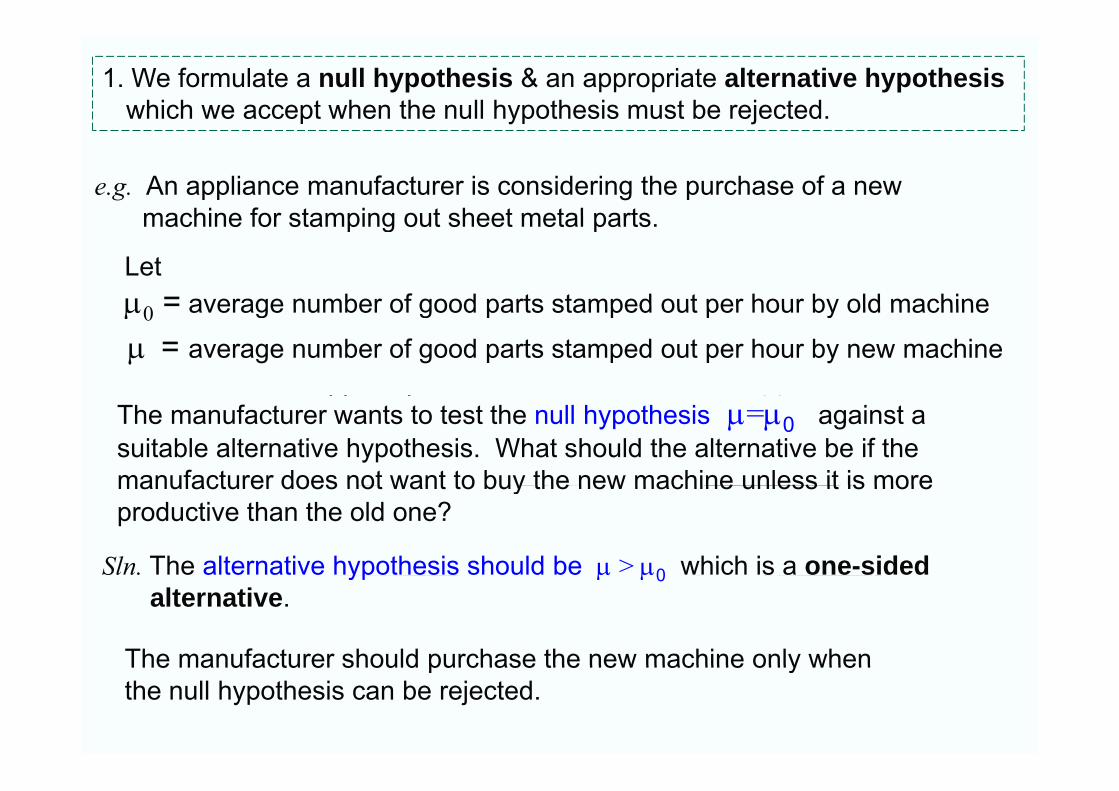
1. We formulate a null hypothesis & an appropriate alternative hypothesiswhich we accept when the null hypothesis must be rejected.

e.g. An appliance manufacturer is considering the purchase of a new machine for stamping out sheet metal partsmachine for stamping out sheet metal parts.

Let = average number of good parts stamped out per hour by old machine

ld hi

0 = average number of good parts stamped out per hour by old machine

= average number of good parts stamped out per hour by new machine

old machine new machineThe manufacturer wants to test the null hypothesis =0 against a suitable alternative hypothesis. What should the alternative be if the manufacturer does not want to buy the new machine unless it is moremanufacturer does not want to buy the new machine unless it is more productive than the old one?

Sln. The alternative hypothesis should be > 0 which is a one-sided yp 0alternative.

The manufacturer should purchase the new machine only whenThe manufacturer should purchase the new machine only when the null hypothesis can be rejected.

2. We specify the probability of a Type I error. If possible, desired, or necessary, we may also specify the probabilities of Type II errors for particular alternatives.

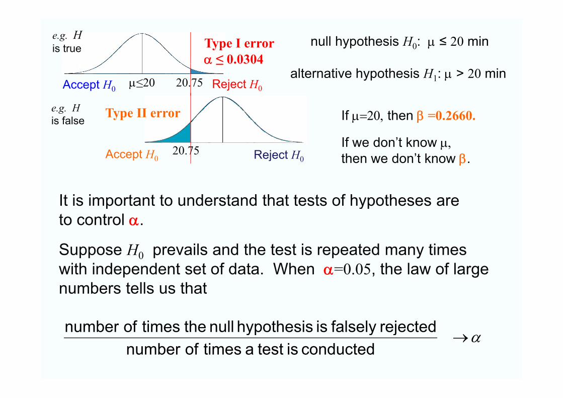
Null Hypothesis H : = 20 min

e.g.1 H is true

yp

= probability of a Type I error= level of significant

0.0304=20 20 75 = level of significant=20 20.75

Accept Hthat =20

Reject Hthat =20 Usually set at 0.05 or 0.01

probability of a Type II error = 0 2660

e.g.2 H is false

We should not specify a Type IType II error =

because that will make the

0.2660

20.75 =21

We should not specify a Type I error that is too small

because that will make the Type II error too big.Accept H

that =20Reject Hthat =20

2. We specify the probability of a Type I error. If possible, desired, or necessary, we may also specify the probabilities of Type II errors for particular alternatives.

Null Hypothesis H: = 20 min Null Hypothesis H: ≤ 20 minAlternative Hypothesis : > 20 min.

Accept H Reject H

y

T I

Correct decision

Type I error

0.0304=20 20 75

e.g.1 His true

≤ 20

Type I error≤ 0.0304

decision error

T II C t

=20 20.75Accept Hthat =20

Reject Hthat =20

≤ 20

Type II error

Correct decision

probability of a Type II error = 0 2660

e.g.2 His false

Type II error = 0.2660

20.75 =21Accept Hthat =20

Reject Hthat =20

3. Based on the sampling distribution of an appropriate statistics, we construct a criterion for testing the null hypothesis against the given g yp g galternative.

e.g.1 H is true

0.0304=20

If the mean of the drying times exceeds 20.75 min, then the claim is rejected20.75

Accept Hthat =20

Reject Hthat =20

then the claim is rejected.If not, the claim is accepted.

20.75

This is called one-sided criterion (one-sided test or one-tailed test).

A test is said to be a two-sided criterion (two-sided test or two-tailed test) if the null-hypothesis is rejected for values of the test statistics falling into either tail of its sampling distributionfalling into either tail of its sampling distribution.


2. We specify the probability of a Type I error. If possible, desired, or necessary, we may2. We specify the probability of a Type I error. If possible, desired, or necessary, we may also specify the probabilities of Type II errors for particular alternatives.

3. Based on the sampling distribution of an appropriate statistics, we construct a criterion for testing the null hypothesis against the given alternative. g yp g g

4. We calculate from the data the value of the statistic on which the decision is to be based.

5. We decide whether to i) reject the null hypothesis or ii) fail to reject it.

Type I error = 0.0304

e.g. His true

=20 20.75Accept H Reject H Instead of selecting the threshold 20.75 subjectively, th ifType II error

=0.2660e.g. His false

the agency may specify values of and to control the risk20.75 =21Accept H Reject Hthe risk.

Type I error = 0.0304

e.g. His true

Instead of selecting the threshold 20.75 subjectively, 0.0304

=20 20.75Accept H Reject H

j y,the agency may specify values of and to control the risk.

Type II error =0.2660

e.g. His false The values could be based on

the consequences of making 20.75 =21Accept H Reject H that kind of errors.

Consequences of making Type I errori) the manufacturer’s cost of having a good product condemned,ii) th f t ’ t f il dj ti hi hiii) the manufacturer’s cost of unnecessarily adjusting his machinery,iii) the cost to the public of not having the product available when needed,

..etc.

Consequences of making Type II errori) the manufacturer’s saving in using inferior ingredients but loss in

d illgood will,ii) the cost to the public of buying an inferior product, … etc.

Type I error ≤ 0.0304

e.g. His true null hypothesis H: ≤ 20 min

≤ 0.0304

≤20 20.75Accept H Reject Halternative hypothesis: > 20 min

In this approach, the maximum value of is controlled over the null h th i F l if th ll h th i i ≤ th

Classical theory of testing hypothesis

hypothesis. For example, if the null hypothesis is ≤ 0, then as well as is unspecified. This is a composite hypothesis.

Otherwise, if all the parameters are completely specified, it is a simple hypothesis.

Because the probability of falsely rejecting the null hypothesis is controlled, the null hypothesis is retained unless the observations strongly contradict it.

Consequently, if the goal of an experiment is to establish a hypothesis, Co seque t y, t e goa o a e pe e t s to estab s a ypot es s,that hypothesis must be taken as the alternative hypothesis.


e.g. His true null hypothesis H0: ≤ 20 min

≤ 0.0304

≤20 20.75Accept H Reject Halternative hypothesis H1: > 20 min

When the goal of an experiment is to establish an assertion, the

Guideline for selecting the null hypothesis

When the goal of an experiment is to establish an assertion, the negation of the assertion should be taken as the null hypothesis. The assertion becomes the alternative hypothesis.

e.g. The goal of the experiment is to establish the assertion that the average drying time of the new “fast-drying”that the average drying time of the new fast drying paint is longer than 20 min so that the agency can issue a warning to the public.

The probability of falsely rejecting the null hypothesis is controlled. In other words the agency can reject the null hypothesis with greatother words, the agency can reject the null hypothesis with great confidence (a controlled or very small type I error).



≤ 0.0304

≤20 20.75Accept H0 Reject H0

alternative hypothesis H1: > 20 min

T IIe g H Type II error

20.75Accept H Reject H

e.g. His false If then =0.2660.

If we don’t know th d ’t k

Notation for the hypothesis

20.75Accept H0 Reject H0 then we don’t know .

H1: The alternative hypothesis is the claim we wish to establish.

H0: The null hypothesis is the negation of the claim.

The errors and their probabilities

Type I error: Rejection of H0 when H0 is true.Type II error: Non-rejection of H0 when H1 is true.= probability of making a Type I error (level of significance)= probability of making a Type I error (level of significance) = probability of making a Type II error



≤ 0.0304

≤20 20.75Accept H0 Reject H0

alternative hypothesis H1: > 20 min

T IIe g H Type II error

20.75Accept H Reject H

e.g. His false If then =0.2660.

If we don’t know th d ’t k

20.75Accept H0 Reject H0 then we don’t know .

It is important to understand that tests of hypotheses areIt is important to understand that tests of hypotheses are to control .

S il d th t t i t d tiSuppose H0 prevails and the test is repeated many times with independent set of data. When =0.05, the law of large numbers tells us thatnumbers tells us that

rejectedfalsely is hypothesisnullthetimes of number

conducted is test a times of numberjyyp

e.g. We want to establish that the thermal conductivity of a certain

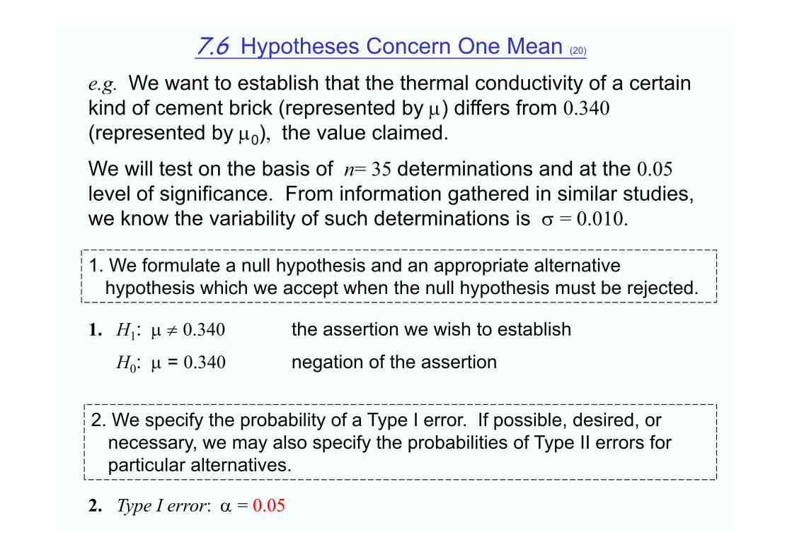
7.6 Hypotheses Concern One Mean (20)

e.g. We want to establish that the thermal conductivity of a certain kind of cement brick (represented by ) differs from 0.340 (represented by 0), the value claimed.

We will test on the basis of n= 35 determinations and at the 0.05level of significance. From information gathered in similar studies, we know the variability of such determinations is 0 010we know the variability of such determinations is = 0.010.


1. H1: 0.340 the assertion we wish to establish

H0: = 0.340 negation of the assertion

2. We specify the probability of a Type I error. If possible, desired, or necessary, we may also specify the probabilities of Type II errors for particular alternatives.particular alternatives.

2. Type I error: = 0.05

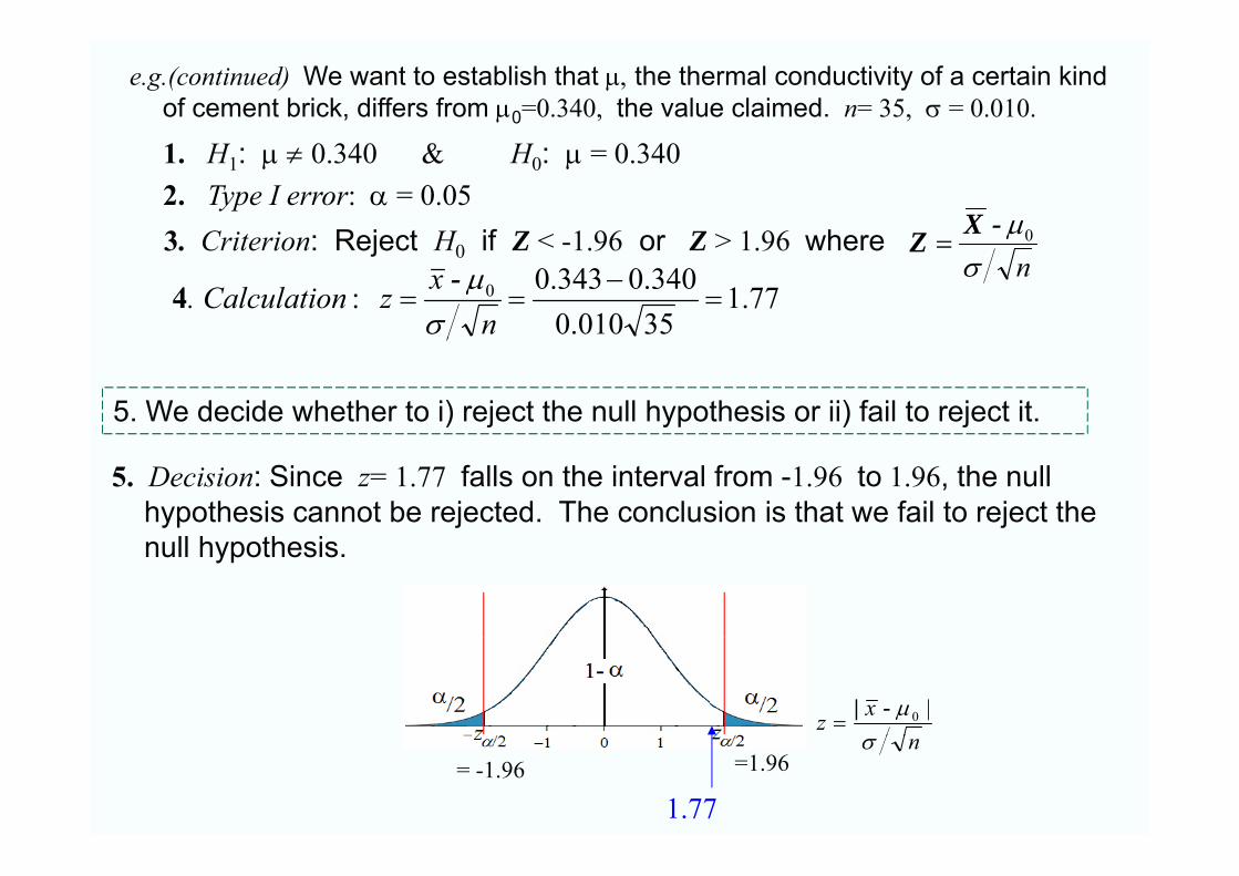
e.g.(continued) We want to establish that the thermal conductivity of a certain kind of cement brick, differs from 0=0.340, the value claimed. n= 35, = 0.010.

1. H1: 0.340 & H0: = 0.3402. Type I error: = 0.05

3. We construct a criterion for testing the null hypothesis against the given alternative.

n0-XZ 3. Criterion: Reject H0 if Z < -1.96 or Z > 1.96 where

= 0.05 so the dividing lines, or critical values, of the criteria are -1.96 and 1.96 for the two-sided alternative.criteria are 1.96 and 1.96 for the two sided alternative.

nxz

|0-|

n

1.96-1.96


1. H1: 0.340 & H0: = 0.3402. Type I error: = 0.05

3. We construct a criterion for testing the null hypothesis against the given alternative.g

alternative hypothesis

reject null hypothesis if

-z Z < -z Z > z

Z < -z or Z > z z

nx

|0-|


1. H1: 0.340 & H0: = 0.3402. Type I error: = 0.05

0-XZ3 Criterion: Reject H if Z < 1 96 or Z > 1 96 wheren0Z 3. Criterion: Reject H0 if Z < -1.96 or Z > 1.96 where

4. We calculate from the data the value of the statistic on which the decision is to be based.

34003430x

Suppose that the mean of the 35 determinations is = 0.343.x

77.135010.0340.0343.0: 0

nx zion. Calculat

-4


1. H1: 0.340 & H0: = 0.3402. Type I error: = 0.05

0-XZ3 Criterion: Reject H if Z < 1 96 or Z > 1 96 wheren0Z 3. Criterion: Reject H0 if Z < -1.96 or Z > 1.96 where

77.135010.0340.0343.0: 0

nx zion. Calculat

-4

5. We decide whether to i) reject the null hypothesis or ii) fail to reject it.

5. Decision: Since z= 1.77 falls on the interval from -1.96 to 1.96, the null hypothesis cannot be rejected. The conclusion is that we fail to reject the

ll h th inull hypothesis.

xz |0-|

n=1.96= -1.96

1.77

5 Decision: Since z= 1 77 falls on the 0 02=0 025

1. H1: 0.340 & H0: = 0.340:

5. Decision: Since z= 1.77 falls on the interval from -1.96 to 1.96, the null hypothesis cannot be rejected.

nxz

|0-|

=1.96= -1.96 1.77

0.025==0.025

The P –value is the probability of obtaining a value for the test statistic P-value for a given test statistic and null hypothesis

that is as extreme or more extreme than the value actually observed.

Probability is calculated under the null hypothesis.

0.0384 0.0384Under the null hypothesis H0: =0.340, obtaining a value for the test statistic that is

z =1.77-1.77The P –value is

obtaining a value for the test statistic that is as extreme or more extreme than the observed value z=1.77 means

0.0768=0.0384+0.0384|Z|≥ 1.77 in this example.

The event that is as extreme or more extreme than that observed may have other meaning.

The P –value is the probability of obtaining a value for the test statistic that is as extreme or more

P-value for a given test statistic and null hypothesis

extreme than the value actually observed. Probability is calculated under the null hypothesis.

0 0384 0 0384alternative hypothesis H1: =0 340

z=1.77

0.0384 0.0384

The P value is 0 0768=0 0384+0 0384

alternative hypothesis H1: 0.340obtaining a value for the test statistic that is as extreme or more extreme than z =1.77 means |Z|≥ 1 77 The P –value is 0.0768=0.0384+0.0384means |Z|≥ 1.77.

alternative hypothesis H1: >,

z=1.77

0.0384alternative hypothesis H1: , obtaining a value for the test statistic that is as extreme or more extreme than z =1.77 means Z ≥ 1 77 The P –value is 0.0384

alternative hypothesis H : <

means Z ≥ 1.77.

alternative hypothesis H1: <, obtaining a value for the test statistic that is as extreme or more extreme than z =-1.77

Z ≤ 1 77z=--1.77

0.0384

means Z ≤ -1.77.The P –value is 0.0384

e.g. We want to establish that the thermal conductivity of a certain kind of cement brick, differs from 0=0.340, the value claimed. n= 35, = 0.010.

1. H1: 0.340 & H0: = 0.3402. Type I error: = 0.05

0-XZ 3 Criterion: Reject H if Z < 1 96 or Z > 1 96 wheren

Z 3. Criterion: Reject H0 if Z < -1.96 or Z > 1.96 where

77.135010.0340.0343.0: 0

nx zion. Calculat

-4

5. Decision: z= 1.77 falls on the interval from -1.96 to 1.96. The conclusion is that we fail to reject the null hypothesis. 1 96 zto reject the null hypothesis. =1.96= -1.96 z = 1.77

The test described above is exact only when the population is normal and is known.

In many practical situations is unknown but sample size n is largeIn many practical situations, is unknown but sample size n is large.

We must make further approximation of substituting by the

.0

nS-XZ sample standard deviation S and so

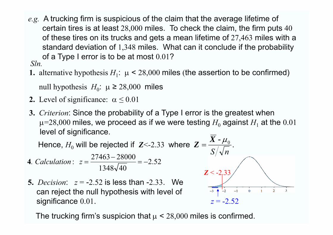
e.g. A trucking firm is suspicious of the claim that the average lifetime of certain tires is at least 28,000 miles. To check the claim, the firm puts 40 of these tires on its trucks and gets a mean lifetime of 27 463 miles with a

Sln

of these tires on its trucks and gets a mean lifetime of 27,463 miles with a standard deviation of 1,348 miles. What can it conclude if the probability of a Type I error is to be at most 0.01?

Sln.1. alternative hypothesis H1: < 28,000 miles (the assertion to be confirmed)

null hypothesis H0: ≥ 28,000 milesyp 0

2. Level of significance: ≤ 0.01

3. Criterion: Since the probability of a Type I error is the greatest when=28,000 miles, we proceed as if we were testing H0 against H1 at the 0.01level of significance.Hence H will be rejected if Z< 2 33 where 0-XZ

Z < 2 33

Hence, H0 will be rejected if Z<-2.33 where

52.2401348

2800027463:

zion. Calculat4

.nS

Z

Z < -2.335. Decision: z = -2.52 is less than -2.33. We

can reject the null hypothesis with level of significance 0.01. z = -2.52

The trucking firm’s suspicion that < 28,000 miles is confirmed.

e.g. A trucking firm is suspicious of the claim that the average lifetime of certain tires is at least 28,000 miles. To check the claim, the firm puts 40 of these tires on its trucks and gets a mean lifetime of 27 463 miles with a standard deviation of 1 348 miles Whatgets a mean lifetime of 27,463 miles with a standard deviation of 1,348 miles. What can it conclude if the probability of a Type I error is to be at most 0.01?

If th l i i ll d i k th t t j tIf the sample size is small and is unknown, the test just described cannot be used.

However, if the sample comes from a normal population (to within a reasonable degree of approximation), we can base the test of the null hypothesis on the statistictest of the null hypothesis on the statistic

nS0-Xt

nS

which is a random variable having the t distribution ith 1 d f f dwith n-1 degree of freedom.

engg2450 probability and statistics for...

Documents