statistical properties of dark matter mini-haloes and ... · amount of hd that forms in primordial...
TRANSCRIPT

Dissertationsubmitted to the
Combined Faculty ofNatural Sciences and Mathematics
of theRuperto-Carola-University of Heidelberg,
Germanyfor the degree of
Doctor of Natural Sciences
Put forward by
M. Sc. Mei Sasakiborn in: Tokyo, Japan
Oral examination: 4 February 2015


Statistical properties of dark matter mini-haloes andthe criterion for HD formation in the early universe
Referees:
Prof. Dr. Ralf S. Klessen
Prof. Dr. Norbert Christlieb


Dedicated to my parents, my sister, and my fiance Takashi Moriya.


Abstract
The aim of this work is to explore how dark matter structures and astronomical ob-jects (the first generation of stars) formed in the high-redshift universe. We investigateproperties of dark matter mini-haloes and clarify the process of primordial star forma-tion that takes place in different dark matter mini-haloes. The specific questions thatwe aim to answer in this work include how dark matter mini-haloes found at z ≥ 15differ from their more massive lower-redshift counterparts and what determines theamount of HD that forms in primordial gas at the initial stage of protostellar collapse.We ran a high-resolution N -body simulation that has the highest mass resolution everachieved for a representative cosmological volume at these high redshifts, and madeprecision measurements of various physical properties that characterise dark matterhaloes. As expected from the differences in the slope of the dark matter densitypower spectrum, the dependence of formation time on dark matter halo mass is veryweak in the case of the haloes that we study here. Despite this difference, dark mat-ter structures at high redshift share many properties with their much more massivecounterparts that form at later times. We ran a separate set of cosmological hydrody-namical simulations to study gas starting to collapse in dark matter haloes. We foundthat in some of our simulated mini-haloes, HD cooling became important during theinitial collapse, and investigated in detail why this occurred. We compared HD-richand HD-poor mini-haloes in our simulations and found that the amount of HD thatforms is linked to the speed of the gravitational collapse. If the collapse is rapid,dynamical heating prevents the gas from cooling to temperatures low enough for HDcooling to become important, but if the collapse is slow, HD cooling can come todominate, resulting in a minimum gas temperature which is lower by a factor of two.We investigated what properties of the mini-haloes were responsible for determiningthe collapse time, and showed that, contrary to previous suggestions, the mass of themini-halo and the rotational energy of the gas appear to have little influence on thespeed of the collapse. We therefore suspect that the main factor determining whetherthe collapse is slow or rapid, and hence whether HD cooling becomes important ornot, is the degree of turbulence in the gas.


Zusammenfassung
Das Ziel dieser Arbeit ist es, die Struktur von Dunkler Materie und astronomischenObjekten (der ersten Generation von Sternen), die im fruhen Universum entstandensind, zu erforschen. Wir untersuchen die Eigenschaften von Dunkle Materie Mini-Halos und den Prozess der primordialen Sternentstehung, der in den verschiedenenMini-Halos stattfindet. Die genauen Fragestellungen, die wir in dieser Arbeit verfol-gen, beinhalten, ob sich Mini-Halos bei einer Rotverschiebung von z ≥ 15 von ihrenmassiveren Gegenstucken zu spateren Zeiten unterscheiden und was die Menge anHD bestimmt, die sich im primordialen Gas am Beginn des protostellaren Kollapsbildet. Wir haben eine hochaufgeloste N -Korper Simulation durchgefuhrt, welche diehochste jemals erreichte Massen-Auflosung in einem reprasentativen kosmologischenVolumen bei dieser hohen Rotverschiebung hat und prazise Messungen von verschiede-nen physikalischen Großen durchgefuhrt, welche die Eigenschaften der Dunkle MaterieHalos charakterisieren. In den hier untersuchten Halos hangt die Entstehungszeit nurschwach von der Masse der Dunkle Materie Halos ab, wie aus den unterschiedlichenSteigungen der Dichte-Leistungsspektren zu erwarten war. Trotz dieses Unterschiedsteilen die Dunkle Materie Strukturen bei hoher Rotverschiebung viele Eigenschaftenmit ihren massiveren Gegenstucken, die spater entstehen. Wir haben zusatzlich eineReihe von kosmologischen hydrodynamischen Simulationen durchgefuhrt, um Gas zuuntersuchen, das gerade beginnt, in den Halos zu kollabieren. In einigen unserersimulierten Mini-Halos wurde Kuhlen durch HD wahrend des anfanglichen Kollapswichtig, und wir verfolgen den Grund dafur im Detail. Aus dem Vergleich von HD-reichen und HD-armen Mini-Halos in unserer Simulation ergibt sich, dass die Mengevon HD, die gebildet wird, mit der Geschwindigkeit des Gravitations-Kollapses zusam-menhangt. Wenn der Kollaps schnell verlauft, verhindert dynamisches Heizen, dassHD-Kuhlen wichtig wird, das erst bei niedrigen Temperaturen einsetzt. Falls derKollaps langsam ist, kann HD-Kuhlen dominant werden, wodurch minimale Gastem-peraturen, die um einen Faktor zwei niedriger liegen, erreicht werden konnen. Wiruntersuchten, welche Eigenschaften der Mini-Halos die Kollapszeit bestimmen, undzeigen, im Gegensatz zu fruheren Erwartungen, dass die Masse und die Rotationsen-ergie wenig bis gar keinen Einfluss auf die Kollaps-Geschwindigkeit haben. Dahervermuten wir, dass der Faktor, der bestimmt, ob ein Kollaps langsam oder schnellverlauft, und damit, ob HD-Kuhlung wichtig wird, der Grad der Turbulenz des Gasesist.

Acknowledgements
To be honest, my PhD experience was one of those that made me consider quitting ona regular basis. I am not sure if I enjoyed doing it—I would have continued astronomythe rest of my life if things worked out a little easier. However, I am certain I couldnot have finished my PhD without the help and encouragement from the followingpeople.
First of all, I would like to express my gratitude to my supervisor, Prof. RalfKlessen, who offered me an opportunity to work on an interesting topic in Heidelberg,for all the support he has offered me through my PhD. He introduced me to manyastronomers, sent me to conferences, thus offering opportunities to interact with manyastronomers, and organised many informal meetings for science discussions. He is afriendly group leader interested in many things, which allows many junior membersof the group to pursue their scientific interest. I cannot thank enough to Dr. SimonGlover and Dr. Paul Clark, for having lots of scientific discussions and being patientand encouraging throughout. Things have been much more difficult if it were not forSimon’s wisdom or Paul’s hacking skills. I learnt a lot from stimulating discussionswith them. Chapter 4 would not have existed without Paul or Simon.
I am also grateful to Prof. Volker Springel, who have offered me the codes that I havebased my scientific work on, and gave me professional pieces of advice. OccasionallyI contacted him for help when I felt I was stuck, and always felt smarter after writingto/discussing with him. If I were to work in a leading position in my future job someday, I would like to treat junior members in the group like Volker does his people. Iwould also like to thank Prof. Matthias Bartelmann, who have offered me valuablepieces of advice especially when I was working on my structure formation paper.He helped me figure out small but important questions in structure formation. He isalways encouraging when I drop in his office to discuss something. The same gratitudegoes to Prof. Bjorn Malte Schafer. I am grateful to Dr. Thomas Greif for offeringhis expertise in the field of primordial star formation and sharing his experience withthe moving mesh code. I also thank Dr. Federico Marinacci for answering my simplequestions on the AREPO code. My sincere thanks also goes to Prof. Norbert Christlieband Prof. Luca Amendola, for being part of my defence committee.
In some respects, I deeply thank my former supervisor, Prof. Naoki Yoshida, forbeing a characteristic supervisor. I probably could not have made up my mind to‘escape’ to Germany to do a PhD if it were not for him. I learnt to maintain sanityand keep struggling even in the most desperate and helpless situations from workingwith him.
This dissertation would have been impossible without financial support from theBaden-Wurttemberg Foundation in the program Internationale Spitzenforschung (con-tract research grant P-LS-SPII/18) or a Distinguished Doctoral fellowship from the

HGSFP.I thank my former and current colleagues in ITA for their friendship including but
not limited to (allow me to dispense with titles): Gustavo Dopcke, Jayanta Dutta,Faviola Molina, Philipp Girichidis, Svitlana Zhukovska, Volker Gaibler, Jon Ramsey,Laszlo Szucs, Joanna Drazkowska, Sebastian Stammler, Sareh Ataiee, Fredrik Wind-mark, Tilman Hartwig, Jennifer Schober, Lukas Konstandin, Juan Ibanez, ChristianBaczynski, Rahul Shetty, Rowan Smith, Erik Bertram, Maria Jimenez, Anna Schauer,Katharina Wollenberg. I am also thankful to the staffs at Caffe MORO for providingus with high quality coffee and also offering us places to waste 15 minutes when wedidn’t feel like working. I thank Sven Weinmann for technical support with com-puters in ITA, and Anna Zacheus and Sylvia Matyssek for administrative support. Ithank the IMPRS coordinator Christian Fendt and all the people from IMPRS, espe-cially from the 7th generation for having fun together. I especially thank Jan Rybizkifor teaching me how to climb, and Salvatore Cielo for hanging around together inconferences and having discussions about dark matter haloes.
I am thankful to all my friends from Japan for wishing me good luck in this en-deavour. I thank my friends from Oin Junior & Senior High School, and friends fromclass of SI-17 in the University of Tokyo for continued friendship. I also greatly thankfellow grad students from Japan for having fun together and also listening to lots ofmy complaints on skype. I am also grateful to former members of Jun Makino’s groupat NAOJ. I thank Yoshimasa Kubo and all other readers of my anonymous blog forsharing their experiences in their PhD program in Europe/US. I think I felt a littleeasier when I realised I am not alone in this struggle towards my PhD degree on theother side of the globe. I hope all of you get a Doctoral degree in the near future.I thank Yumi Chang, my best friend from Karachi American School for continuedfriendship.
I am grateful to my parents and my sister for being supportive throughout. It wasassuring to know that there is always one place I can go back to.
I am thankful to my fiance Takashi Moriya for being with me since we were un-dergrads, for all the support and patience he has offered me despite the long distancebetween Heidelberg and Japan in the first 2.5 years in my PhD, and also for makinga lot of effort in being with me and eventually finding a post-doc position in Bonn.This thesis has been impossible without him.
List of publications
Refereed publications
• Sasaki, Mei, Clark, Paul C., Springel, Volker, Klessen, Ralf S., Glover, Si-mon C. O. Statistical properties of dark matter mini-haloes at z >= 15, 2014,Monthly Notices of the Royal Astronomical Society, Volume 442, Issue 3, p.1942-1955
• Sasaki, Mei, et al. 2015. The criterion for HD formation in the early universe- in prep.
Conference proceedings
• Sasaki, Mei, Clark, Paul C., Klessen, Ralf S., Glover, Simon C. O., Springel,Volker, Yoshida, Naoki. Statistical properties of dark matter mini-halos, 2012,FIRST STARS IV - FROM HAYASHI TO THE FUTURE -. AIP ConferenceProceedings, Volume 1480, pp. 409-411


Contents
1 Introduction 11.1 CDM universe . . . . . . . . . . . . . . . . . . . . . . . . . . . . . . . . 1
1.2 Equations that govern the density peak evolution in the universe . . . 2
1.3 Power spectrum, transfer function, initial conditions . . . . . . . . . . 3
1.4 Spherical collapse model . . . . . . . . . . . . . . . . . . . . . . . . . . 5
1.5 Press-Schechter mass functions . . . . . . . . . . . . . . . . . . . . . . 7
1.6 N -body simulations . . . . . . . . . . . . . . . . . . . . . . . . . . . . 8
1.7 Relaxation time . . . . . . . . . . . . . . . . . . . . . . . . . . . . . . . 9
1.8 Identification of structure in cosmological simulations . . . . . . . . . . 12
1.9 Condition for star formation . . . . . . . . . . . . . . . . . . . . . . . . 12
1.10 Pop III - Pop II transition . . . . . . . . . . . . . . . . . . . . . . . . . 14
1.11 Reactions involving H2 in the primordial gas . . . . . . . . . . . . . . 15
1.12 Protostellar collapse . . . . . . . . . . . . . . . . . . . . . . . . . . . . 16
1.13 Accretion phase . . . . . . . . . . . . . . . . . . . . . . . . . . . . . . . 16
1.14 Observational signatures . . . . . . . . . . . . . . . . . . . . . . . . . . 18
1.15 Structure of this thesis . . . . . . . . . . . . . . . . . . . . . . . . . . . 20
2 Small-scale structure formation 212.1 Introduction . . . . . . . . . . . . . . . . . . . . . . . . . . . . . . . . . 21
2.2 Methods . . . . . . . . . . . . . . . . . . . . . . . . . . . . . . . . . . . 23
2.2.1 Merger trees . . . . . . . . . . . . . . . . . . . . . . . . . . . . 24
2.3 Results . . . . . . . . . . . . . . . . . . . . . . . . . . . . . . . . . . . . 24
2.3.1 Spin parameter . . . . . . . . . . . . . . . . . . . . . . . . . . . 26
2.3.2 Virial ratios . . . . . . . . . . . . . . . . . . . . . . . . . . . . . 27
2.3.3 Mass function . . . . . . . . . . . . . . . . . . . . . . . . . . . . 30
2.3.4 Formation time . . . . . . . . . . . . . . . . . . . . . . . . . . . 32
2.3.5 Halo shape . . . . . . . . . . . . . . . . . . . . . . . . . . . . . 33
2.3.6 Correlation between formation time and virial ratio / formationtime and halo shape . . . . . . . . . . . . . . . . . . . . . . . . 36
2.3.7 Correlation function . . . . . . . . . . . . . . . . . . . . . . . . 38
2.4 Conclusions . . . . . . . . . . . . . . . . . . . . . . . . . . . . . . . . . 40
3 Improving the Arepo code 453.1 Numerical methods . . . . . . . . . . . . . . . . . . . . . . . . . . . . . 45
3.2 Technical challenges . . . . . . . . . . . . . . . . . . . . . . . . . . . . 48
3.3 Results . . . . . . . . . . . . . . . . . . . . . . . . . . . . . . . . . . . . 49
3.3.1 Idealised tests . . . . . . . . . . . . . . . . . . . . . . . . . . . . 49
xv

Contents
3.3.2 Collapse tests . . . . . . . . . . . . . . . . . . . . . . . . . . . . 54
4 HD formation 614.1 Introduction . . . . . . . . . . . . . . . . . . . . . . . . . . . . . . . . . 614.2 Numerical methods . . . . . . . . . . . . . . . . . . . . . . . . . . . . . 634.3 Results . . . . . . . . . . . . . . . . . . . . . . . . . . . . . . . . . . . . 634.4 Numerical convergence . . . . . . . . . . . . . . . . . . . . . . . . . . . 694.5 Conclusion . . . . . . . . . . . . . . . . . . . . . . . . . . . . . . . . . 69
5 Conclusion 735.1 Small-scale structure formation . . . . . . . . . . . . . . . . . . . . . . 735.2 Criterion for HD formation in primordial gas . . . . . . . . . . . . . . 74
A Appendix 75A.1 Comparison of structure formation simulation at large and small scales. 75A.2 Influence of particle numbers on calculating sphericity parameter. . . . 77A.3 Resolution study of the non-dimensional spin parameter . . . . . . . . 79A.4 Non-dimensional spin parameter calculated for FOF haloes . . . . . . 80A.5 Density slice through the whole box. . . . . . . . . . . . . . . . . . . . 80
Bibliography 83
xvi

1 Introduction
Where did we come from? Where are we going? Thanks to the advances in naturalsciences, scientists today can do a much better job in answering such fundamentalquestions than in the past. We have a common understanding that the universe wasmuch smaller in size, hotter, and denser when it was born in a Big Bang about 13.8Gyrs ago, and that it continues to expand at an increasing rate. We also know that thefirst generation of stars contributed significantly in changing the simple homogeneousstate of the universe at the time of its birth to the more complex and diverse state asit is today.
The goal of this thesis is to make a small advancement in the fields of first starformation and structure formation.
Stars are divided into three populations according to the amount of ‘metals’, i.e.elements heavier than lithium (Li) they contain: Population I (metal-rich), Popu-lation II (metal-poor), and Population III (metal-free). Since metals did not existimmediately after the Big Bang, the first stars to form in the universe were Popu-lation III (Pop III) stars. Once the Pop III stars have formed, at the end of theirlives, elements synthesised at the centres of the stars were distributed by supernovaexplosions. Therefore, it is believed that there is a gradual transition from Pop III toPop II stars. Pop II stars are most often found in the bulge and halo of galaxies. PopI stars are mostly found in the disks of galaxies. The Sun is an example of a Pop Istar.
In this chapter, we will first summarise the key concepts in structure formation.Then we will briefly explain baryonic physics which is relevant for Pop III star forma-tion.
1.1 CDM universe
If we consider the line element ds of the form
ds2 = gµνdxµdxν , (1.1)
under the assumptions of homogeneity and isotropy, we arrive at the below metric(Robertson-Walker metric):
ds2 = −c2dt2 + a2(t)
[dr2
1−Kr2+ r2(dθ2 + sin2 θdφ2)
]. (1.2)
The Einstein’s equations read
Rµν −1
2Rgµν + Λgµν =
8πG
c4Tµν , (1.3)
1

1 Introduction
where Rµν is the Ricci tensor, R (= gµνRµν) is the Ricci scalar, Λ is the cosmologicalconstant, and Tµν is the energy-momentum tensor (T00 = ρc2, Tij = pδij where 1 ≤i, j ≤ 3). Substituting this metric (equation (1.2)) in the Einstein equations (equa-tion (1.3)) we obtain Friedman equation,
H(a)
H0=
√Ωr
a4+
Ωm
a3+
ΩK
a2+ ΩΛ
H(a) = a/a
(1.4)
where ΩK = −Kc2/H20 , ΩΛ = Λc2
8πG/ρcr,0, and Ωm (Ωr) denotes the density of matter(radiation) scaled by critical density of the universe at present, ρcr,0 = 3H2
0/8πG. Thisequation tells us the scale factor a at a given time. It is used to convert scale factorand physical time inside our cosmological simulations. The phases usually studied byN -body or hydrodynamical simulations is either matter-dominated or cosmological-constant-dominated era (meaning either the term Ωm/a
3 or the term ΩΛ is dominantin the rhs of equation (1.4)), therefore, the radiation and curvature terms are ac-tually not included in the code. The precise values of the cosmological parametersthat appear in these equations are known, for example, by measuring the height andlocations of peaks in the angular power spectrum of anisotropies in cosmic microwavebackground (Komatsu et al., 2011). We know that a large portion of the matter com-ponent of Friedmann equations is cold dark matter (CDM), meaning that the velocitydispersions of the dark matter particles at the time they became non-relativistic wasnot big enough to erase the density perturbations already present at that time.
1.2 Equations that govern the density peak evolution in theuniverse
If we rewrite the continuity equation and equation of motion in comoving coordinates,it reads:
∂ρ
∂t+ 3Hρ+∇ · (ρu) = 0 (1.5)
∂u
∂t+ 2Hu + (u · ∇)u = − 1
a2∇(φ+
1
2aax2
)− ∇pa2ρ
, (1.6)
where r is the physical coordinates, x = r/a is comoving coordinates, and u = xis the velocity in comoving coordinates, ρ is the density, p is the pressure, φ is thegravitational potential. The gravitational potential φ is given by Poisson equation,which is expressed in the following equation when differentiated in proper coordinates,
4 φ = 4πGρ. (1.7)
There is no general analytical solution for this equation. When the density pertur-bations are still small, it is possible to perturb equations (1.5) and (1.6) and keep onlylinear terms to follow the evolution of density peaks. Of course, for the dark matter
2

1.3 Power spectrum, transfer function, initial conditions
component, the last term in equation (1.6) is not present. Let us define density per-turbation by δ(x) ≡ (ρ(x)− ρ)/ρ where ρ is the background density at a given time.Then, in the linear regime, if we assume δ(x) ∝ exp(ik · x), the evolution of δ(x) isdescribed by
∂2δ
∂t2+ 2H
∂δ
∂t−(
4πGρ− c2sk
2
a2
)δ = 0. (1.8)
This shows that the modes with 4πGρ− c2sk
2/a2 > 0 keeps growing in the presenceof a small initial positive perturbation. This corresponds to density perturbationswith wavelength λ ≡ 2π/k > cs/a
√π/Gρ, or in proper wavelength, λp > cs
√π/Gρ
(the Jeans length, see also Section 1.9). However, this tactics would not work whenthe density perturbations have grown too big.
1.3 Power spectrum, transfer function, initial conditions
The power spectrum for density perturbations is given by
P (k) = 〈|δk|2〉, (1.9)
where δk is the Fourier transformation of density perturbation δ(x). In fact, thepower spectrum is a variable with dimensions of (length)3, and to evaluate its value,the non-dimensional quantity
∆2(k) ≡ k3P (k)
2π2(1.10)
is used. We can write d3kP (k)/(2π)3 = d ln k∆2(k) assuming isotropy and thusreplacing the integral d3k by 4πk2dk. Therefore, equation (1.10) shows the powerpresent in a logarithmic bin.
The initial conditions for our cosmological simulations are generated in the followingway:First the linear power spectrum is given by
P (k) = A k T (k)2, (1.11)
where A is the normalisation factor, which depends on both cosmological parametersused and the redshift the power spectrum is calculated. T (k) gives the amplitude ofdensity perturbations relative to the largest scales (e.g. normalised such that T (k)→ 1as k → 0). This transfer function has the approximate form of
T (k)
1 (k kH(teq))k−2 (k kH(teq))
, (1.12)
where kH(teq) denotes the wavenumber that corresponds to the Hubble radius (rH ≡c/H) at the time of matter-radiation equality (meaning when Ωr/a
4 = Ωm/a3 in
equation (1.4)). For the density perturbations that ‘enter the horizon’ (i.e. wavelength
3

1 Introduction
Figure 1.1: The linearly extrapolated power spectrum of dark matter at z = 0 for thecosmological parameters adopted in Sasaki et al. (2014) and in Chapter 2.The critical slope of k−3 is shown with dark blue line.
becomes equal to the Hubble radius) in the radiation-dominated era, the densityperturbations stop growing. This functional form accounts for the fact that the modesthat enter the horizon earlier (smaller modes) are more suppressed. As a result of thisk-dependence in the transfer function, the power spectrum of density perturbationshave a turnover (see Fig. 1.1).
The exact functional form of T (k) often used are,
T (k) =
1 +[ak + (bk)3/2 + (ck)2
]ν−1/ν, (1.13)
where
a = 6.4(Ω0h2)−1 (1.14)
b = 3.0(Ω0h2)−1 (1.15)
c = 1.7(Ω0h2)−1 (1.16)
ν = 1.13, (1.17)
as derived by Bond and Efstathiou (1984) and
T (k) = T0(q) =L0
L0 + C0q2, (1.18)
with L0(q) and C0(q) of the form
L0(q) = ln(2e+ 1.8q), (1.19)
C0(q) = 14.2 +731
1 + 62.5q, (1.20)
4

1.4 Spherical collapse model
where q = k/hMpc−1Θ22.7Γ, with Γ = Ω0h and Θ2.7 = TCMB/2.7 [K] as derived by
Eisenstein and Hu (1998) (note that we followed the notation of the original paperand used Ω0 instead of Ωm here). The latter is used for generating initial conditionsfor simulations presented in Chapter 2. For the initial condition generator we used,it is also possible to adopt an arbitrary form of transfer function that is provided bythe user.
Then by applying Fourier transform, it is possible to get particle dispositions inreal space that has a Power spectrum P (k).
The transfer functions that are used here are valid when the density perturbationsare still small (δ(x) ∼ 1). However, we need different methods to probe the densestregions in the universe at later times. Therefore, this prescription is widely used togenerate initial conditions (particle distributions for N -body simulations) in the earlyuniverse when the density is uniform. We find the evolution of dense structures laterin cosmic history by numerically integrating the equation of motion over time.
1.4 Spherical collapse model
The simplest model to explain formation of dense structures is the spherical collapsemodel. We here consider time evolution of spherically symmetric density perturba-tions with radius R(t) that contains total mass of M (= const.)
d2R
dt2= −GM
R2. (1.21)
Time integrating equation (1.21), we obtain
(dR
dt
)2
=2GM
R+ 2E, (1.22)
where E is an integration constant. We see from equation (1.22) that the sign of Edecides on the fate of this sphere. If E > 0, then the rhs of equation (1.22) is always> 0, and the radius of sphere will monotonically increase (non-bound solution). IfE < 0, then initially the rhs of equation (1.22) is > 0, however, at R = −GM
E ,becomes equal to 0, and the expansion of R(t) stops, and after that, the sphere startsto fall inside (bound solution). Therefore, depending on the initial state, there aretwo different kinds of regions inside the universe. Those with E > 0 that continue toexpand, and those with E < 0 that stop to expand and starts to fall back at somepoint.
The solutions to these equations are given in the formR = A2(1− cos θ)
t = A3√GM
(θ − sin θ)(E < 0) (1.23)
R = A2(cosh θ − 1)
t = A3√GM
(sinh θ − θ) (E > 0) (1.24)
5

1 Introduction
where A is an integration constant and θ is the intervening variable.For the bound solution, the maximum value in R(t) is achieved (the sphere stops
expanding) when θ = π. According to equation (1.23) this is when
tturn =πA3
√GM
, Rturn = 2A2 (1.25)
and the sphere collapses to a point when θ = 2π
tcoll =2πA3
√GM
, Rcoll = 0. (1.26)
From the above equation, if we adopt an Einstein-de Sitter universe (Ωm = 1,Ωr =ΩΛ = ΩK = 0 in equation (1.4)) for simplicity, then the background density is givenby ρ = 1/(6πGt2). Substituting the density inside the sphere, ρ = M/(4πR3/3),density perturbations (= ρ/ρ− 1) can be formulated as
δ(t) =9GMt2
2R3− 1 =
92
(θ−sin θ)2
(1−cos θ)3− 1(E < 0)
92
(sinh θ−θ)2(cosh θ−1)3
− 1(E > 0)(1.27)
If we consider that the sphere virializes between the turn around point and the col-lapse point, then the kinetic energy and potential energy at this virialization satisfies
2Kvir + Uvir = 0 (virial equilibrium) (1.28)
and
Kvir + Uvir =3
5GM2
Rturn(energy conservation). (1.29)
We assumed constant density inside the sphere in deriving equation (1.29). Thus weobtain
Uvir =6
5GM2
Rturn=
3
5G
M2
Rturn/2. (1.30)
Therefore, when virialized, the radius of the sphere is Rvir = Rturn/2 = A2, whenθ = 3π/2. The time required for the mass inside the sphere to virialize is the order oftcoll, therefore, the density perturbation at this point is
δvir =M/(4πR3
vir/3)
ρ(tcoll)− 1 = 18π2 − 1 ' 177. (1.31)
In the spherical model, gravitationally collapsed regions have density contrast of ∼177 compared to the mean background density. Even if we adopt different cosmologies,this resulting value changes little (Peebles, 1980). Inspired by this spherical collapsemodel, the overdensity of 200 is widely used as a threshold to identify virializedregions in three-dimensional collisionless simulations intended to follow the structure
6

1.5 Press-Schechter mass functions
formation in a cosmological context. ρ200 (R200) is often used to represent the density(radius) of such regions.
Let us look at the spherical collapse model when the density perturbations are stillsmall and compare it with linear theory. By expanding equation (1.27) in terms of θ,we obtain
δ =3
20θ2 +O(θ4) (1.32)
t =A3
6√GM
θ3 +O(θ5) (1.33)
To lowest order, δ ∝ t2/3. If we note linear density perturbation by δL, we can write
δL(t) =3
20
(6√GM
A3t
)2/3
. (1.34)
To compare values of δ and δL, the linear density perturbations at the point of collapseis
δL(tcoll) =3(12π)2/3
20' 1.69. (1.35)
The Press-Schechter theory explained in the next section is based on the idea thatonce the linear density perturbations reach the value of 1.69, the structure has formed.
1.5 Press-Schechter mass functions
We hereby describe a popular analytical model to predict the number of objects withcertain mass (Press and Schechter, 1974).
In this model, the critical value of density perturbations to form astronomical ob-jects are assumed to be δc ' 1.69, which is taken from a spherical collapse model (seeSection 1.4).
If we assume that the density perturbations follow a Gaussian distribution, thenthe probability distribution function for the density perturbations averaged over massof M is expressed as
P (δM )dδM =1√
2πδ2(M)exp
(−
δ2M
2σ2(M)
). (1.36)
The assumption of Gaussianity is reasonable since recent measurements in the cosmicmicrowave background suggest very low non-Gaussianity (Planck Collaboration et al.,2014) and most simple form of inflation theory predicts Gaussian density perturba-tions. Even if the density perturbations are not exactly Gaussian, we can considerthem as sums of a large number of different modes in k-space that are independentof each other, which, by the central limit theorem, suggests that the density pertur-bations in real space approach asymptotically to a Gaussian distribution.
7

1 Introduction
Therefore, the fraction that exceeds the critical value when averaged over a regionwith mass M is
P>δc(M) =
∫ ∞δc
P (δM )dδM =1√2π
∫ ∞δc/σ(M)
e−x2/2dx, (1.37)
where σ(M) is the overdensity in a sphere of mass M and given by
σ(M) ≡∫dx′δ(x′)WR(x− x′), (1.38)
where WR and R is defined by
WR(x) =
1 (|x| < R)0 (|x| > R)
, M =4π
3R3ρ. (1.39)
If we represent the number of objects with masses between M and M + dM per unitvolume by n(M)dM , and multiply the rhs by a factor of 2 to account for mass thatreside in under-dense regions, we arrive at
n(M)MdM = 2ρ
∣∣∣∣dP>δcdM
∣∣∣∣ dM. (1.40)
Combining equations (1.37) and (1.40), we obtain the following equation:
n(M) =
√2
π
ρ
M2
∣∣∣∣d lnσ(M)
d lnM
∣∣∣∣ δcσ(M)
exp
(− δ2
c
2σ2(M)
). (1.41)
This is known to be in good match with the results of numerical simulations for abroad mass range. For the mass function at the smallest mass ranges, see the plot inChapter 2.
1.6 N-body simulations
N -body simulations are the primary tool to investigate the formation of gravitation-ally bound objects in the universe, once the density perturbations have become solarge that the perturbation theory does not work. (See Section 1.3 for one definitionwhen the density perturbation is large.) In this approach, by using large number ofparticles, the acceleration due to gravitational force is obtained for each particle byadding up contributions from all other particles. Perhaps this is conceptually themost straightforward way to follow the evolution of collisionless self-gravitating sys-tems and thus has a long history. There are in principle other ways such as solving theBoltzmann equation in phase space (Yoshikawa et al., 2013). Note this is an expensiveoperation that scales as O(N6)(!) for 3D case.
In modelling the smooth underlying dark matter distribution with a finite num-ber of particles in the simulation, in order to prevent artificial two-body interactions,softening length ε is widely used in the field to smooth gravitational forces when two
8

1.7 Relaxation time
particles become too close to each other. Suppose we are calculating the gravitationalforce between i-th particle and j-th particle, the gravitational force proportional to
1|ri−rj |2 is modified to 1
|ri−rj |2+ε2, where ri and rj represent the positions of the par-
ticles in proper coordinates. ε is typically set to a few percent of the mean particleseparation in the simulation box.
In order to calculate gravitational forces that work on particles, it is necessary tosum up contributions from all other particles for each timestep. This is an O(N2)calculation, and can become increasingly time-consuming as the number of particlesincreases. The astrophysical community has developed several ways to solve thisproblem. Calculating the gravitational force is much more expensive in terms of com-putational time than in any other operations in many-body simulations. One solutionis to build a special purpose computer dedicated to accelerate this operation (Makinoet al., 1997). Another way is to reduce the cost of force calculation by groupingparticles far away from the particle on which we are to calculate the gravitationalforces (for example, tree method; originally from Barnes and Hut 1986). This methodscales as O(N logN). However, even with special purpose computer, the maximumnumber of particles we can plausibly solve by direct summation is ∼ 106 (Makino,2002). Therefore in modern structure formation simulations, approximate methodsto reduce the cost of force calculation is essential.
1.7 Relaxation time
Following the discussions of Binney and Tremaine (2008) and lecture slides for anastrophysical school1, let us consider a system that consists of N particles (‘stars’)with mass m, and estimate the time it takes for a star for its velocity to be changedsignificantly by encounters with other stars. Here we would like to estimate thetimescale at which we start to see numerical artifacts resulting from the discretisationof the underlying smooth dark matter density field by finite number of particles inour N -body simulations. We would like to study the change of velocity of a pointmass (‘subject star’) with uniform mass m by an encounter with another point mass(‘field star’). If we assume that the subject star travels along a straight trajectorywhile passing along the field star with speed v, impact parameter b, that the positionof the field star does not change throughout this encounter, and that the change invelocity is small (|δv|/v 1) (see how we defined the coordinates in Fig. 1.2), thenthe perpendicular component of the force on the subject star can be written as
F⊥ =Gm2
b2 + x2cos θ =
Gm2b
(b2 + x2)3/2=Gm2
b2[1 + (vt/b)2
]−3/2. (1.42)
The parallel component of force vanishes when integrated over time.
By time integrating this force (setting the origin of time to the moment of closest
1http://obswww.unige.ch/lastro/conferences/sf2013/pdf/lecture1.pdf
9

1 Introduction
r
bx
F⊥
θ
Figure 1.2: Coordinates adopted in calculating the velocity change of the subject star.The subject star is represented with a blue circle, the field star with a redcircle. The trajectory of the subject star is demonstrated with a solid linehere.
approach of two stars), the change in velocity is
δv =1
m
∫ ∞−∞
dtF⊥ =GM
b2
∫ ∞−∞
dt
[1 + (vt/b)2]3/2
=Gm
bv
∫ ∞−∞
ds
(1 + s2)3/2=
2Gm
bv.
(1.43)
The assumption that the change in velocity is small breaks down when δv ' v (*),namely, when b . 2Gm/v2. The typical speed v of field star is given by
v2 ≈ GNm
R. (1.44)
Substituting equation (1.44) to expression (*), we find that the minimum value allowedfor the impact parameter is bmin = 2R/N .
Suppose N stars are located in a disk of radius R. The surface density of stars isN/(πR2), and therefore the expected number of encounters for this subject star percrossing with impact parameter in the range b and b+ db is
dn =N
πR22πbdb =
2N
R2bdb (1.45)
By adding up different encounters, after one crossing, the change in mean-squarevelocity becomes
(∆v)2 =
∫ (2Gm
bv
)dn = 8N
Gm2
Rv
∫db
b= 8N
Gm2
Rvln Λ, (1.46)
10

1.7 Relaxation time
where
ln Λ ≡ ln
(bmax
bmin
). (1.47)
Using equation (1.44) to eliminate R in equation (1.46), we get
(∆v)2
v2≈ 8 ln Λ
N(1.48)
Since equation (1.48) gives the change in velocity after one crossing, the number ofcrossings nrelax that is required for the velocity of subject star to change by of orderitself is
nrelax 'N
8 ln Λ. (1.49)
The relaxation time is defined as trelax = nrelaxtcross, where tcross = R/v, therefore,
trelax =N
8 ln Λtcross. (1.50)
Now if we evaluate the minimum and maximum value for the impact parameter,
bmax = R, (1.51)
bmin =2R
N, (1.52)
Λ = lnR
2R/N= ln
(N
2
), (1.53)
thus we obtain
trelax 'N
8 lnNtcross. (1.54)
If we replace stars by dark matter particles, this equation can be used to evaluatethe relaxation time for dark matter haloes in structure formation simulations. Herewe consider the region that is factor of 200 denser than the critical density (this isfrom analogy with the spherical collapse model, see Section 1.4 for an explanation ofwhy regions ∼ 200 times denser than the background density is relevant). It followsfrom
M200 =4π
3200ρcritR
3200, (1.55)
v200 =
√GM200
R200, (1.56)
and
ρcrit =3H2
8πG(1.57)
11

1 Introduction
that
tcross 'R200
v200∼ 1
2H. (1.58)
Plugging equation (1.58) into equation (1.54) yields
trelax 'N
16 lnN
(1
H
), (1.59)
which shows, for systems that is reasonably well resolved (N > 100), relaxation timeis longer than the age of the universe (∼ 1
H ), and that the output of our collisionlesssimulations are not just artifacts resulting from two-body interactions.
1.8 Identification of structure in cosmological simulations
In a simulation using collisionless particles to represent dark matter density, themethod to identify structures that have formed inside the simulation domain canbe problematic. Different groups have adopted different methods and this is one ofthe factors that make comparison of the works from different groups difficult. Mostof the structure-finding algorithms adopted today are descendants of either of the twomethods: the friends-of-friends (FOF) method (Davis et al., 1985) and the spherical-overdensity (SO) method (Lacey and Cole, 1994). Methods based on SO first identifydensity peaks, and then grow shells around these peaks until the density drops undersome predefined lower limit. This limit is usually taken from the spherical collapsemodel. Methods based on FOF tries to link together particles that are located closeto each other (either in 3D space or in 6D phase-space). In the work presented inChapter 2, an additional algorithm to spot dense regions inside FOF haloes is used(SUBFIND). A summary of various different approaches to identify structures is givenin Knebe et al. (2013). They find that when comparing properties of correspond-ing objects identified by different algorithms, directly measurable properties such asposition, bulk velocity, maximum velocity have scatter of only a few percent, whilederived properties such as shape or spin have a much larger scatter. For an exam-ple on how halo identification affects the value of spin parameter, compare Fig. 2.3with A.5. Measuring the shape of haloes (i.e. fitting the particle distribution withan ellipsoid) is difficult, because the shape of haloes we find in structure formationsimulations are not exactly ellipsoids. Instead, their shapes change as a function ofradius (we checked that for the data analysed in Chapter 2, the inner parts of thehalo are more spherical).
1.9 Condition for star formation
In Fig. 1.3, the cooling functions for various elements in atomic gas with solar com-position is shown. In the early universe, when the first generation of stars form in aregion where there was no preceding generations of stars, elements heavier than Li areabsent. Therefore most of the elements relevant for cooling in the local interstellarmedium (ISM) (e.g. C+, Si+, Fe+, O, S+) are absent. Cooling due to atomic hydrogen
12

1.9 Condition for star formation
Figure 1.3: Cooling functions of various elements weighted by their abundance. Takenfrom Fig.1 in Dalgarno and McCray (1972)
Figure 1.4: Cooling function of H atom and He atom in primordial gas. Taken fromFig.1 in Nishi (2002)
13

1 Introduction
and atomic helium is effective only at T > 104 K (Nishi, 2002, and Fig. 1.4). In sucha case, H2 line cooling is the primary physical process that lowers the temperaturesof gas to T 104 K.
In order for the gas to start collapsing inside the centres of the dark matter haloes,several conditions have to be met.
In Section 1.2 we introduced the Jeans length in a cosmological context, however,the formulation is the same even in proper coordinates. Thus, the minimum gas massin haloes required to start a run-away collapse (the Jeans mass) is:
MJ ≡ 4π
3ρ
(λJ
2
)3
, (1.60)
where
λJ = cs
√π
Gρ. (1.61)
Otherwise, the collapse will be halted by the internal pressure.For T = 200 K, n = 104 cm−3, the Jeans mass is > 100 M. The clump with this
mass may fragment into smaller pieces later in the collapse, so this mass cannot bedirectly associated with the masses of resulting stars.
The criterion tcool = ε/ε ∼ 32nkT/Λ(T ) < tff ∼ 1√
Gρ, tH ≡ a/a also has to be
met (Tegmark et al., 1997), where T is the temperature of gas, Λ represents coolingfunction, and ε represents the thermal energy. This gives a minimum mass of the halofor primordial gas to collapse inside it. The exact lower mass depends on the reactionrates adopted. However, by assuming the virial temperature of primordial gas to be1000 K, Glover (2013) calculates the critical halo mass as:
Mcrit ' 6× 10⁵h−1( µ
1.2
)−3/2Ω−1/2m
(1 + z
10
)−3/2
. (1.62)
If this condition is not met, the gas collapse is either prevented by thermal pressureor the expansion of the universe. Yoshida et al. (2003) has shown this explicitly withdirect hydrodynamical simulations in a cosmological context. The latter also suggeststhat dynamical heating from mergers could delay the initial collapse of primordialgas.
1.10 Pop III - Pop II transition
The transition in the characteristic mass for different populations of stars can beunderstood to lowest order by the argument of Jeans masses. As heavy elementsproduced inside the stars and dust that is formed out of these metals are distributedto the interstellar medium, there are more coolants and the Jeans masses becomelower.
There are two main theories about the main driver for transition from Pop III toPop II stars. There are works that argue C+ and O produced as a result of earlier
14

1.11 Reactions involving H2 in the primordial gas
Figure 1.5: Thermal evolution of gas with different metallicities. The second troughin temperatures is induced by dust cooling. Taken from Fig.1 in Omukai(2000)
generation of stars lowers the characteristic masses of Pop II stars (Bromm et al., 2001;Bromm and Loeb, 2003; Santoro and Shull, 2006). Theoretically, there is a concept of‘critical metallicity’, Zcrit, above which the mode of star formation changes from PopIII stars to Pop II stars. In this theory, the critical metallicity Zcrit is found to be∼ 10−3Z. On the other hand, Omukai (2000) and Schneider et al. (2003) emphasisesthe importance of dust, which could be produced from supernova explosions of thefirst stars (Todini and Ferrara, 2001; Nozawa et al., 2003). They followed the thermalevolution of gas with different metallicities and demonstrated that the dust grains aremostly responsible for the fragmentation which is taking place in the enriched gas(see Fig. 1.5). Based on works of Clark et al. (2008), Dopcke et al. (2011, 2013) haveimproved on the treatment of dust and found formation of low-mass stars. For thisdust cooling scenario, Zcrit = 10−6 − 10−4 Z is considered to be capable of changingthe characteristic mass of stars.
1.11 Reactions involving H2 in the primordial gas
As discussed in Section 1.9, H2 plays an important role in the cooling of the metal-freegas. In primordial gas, the chemical reactions that is relevant for the formation of H2
at densities higher than ∼ 108 cm−3 is
H + H + H→ H2 + H, (1.63)
15

1 Introduction
as can be seen from the fact that the speed at which this reaction proceeds increasesrapidly as density increases (proportional to the cube of number density of hydrogenatoms).
Other important channels in which H2 forms at lower densities are
H + e− → H− + γ (1.64)
H− + H → H2 + e− (1.65)
and
H + H+ → H+2 + γ (1.66)
H+2 + H → H2 + H+. (1.67)
The processes presented here are less efficient than H2 formation in the local interstel-lar medium, where H2 molecules typically form on dust grains. In the absence of dustgrains, H + H → H2 + γ is an inefficient process since H2 molecules cannot radiateaway excess energy because they do not possess a dipole moment.
1.12 Protostellar collapse
The capital letters in square brackets in this paragraph represent different points in theρ-T diagram demonstrated in Fig. 1.6 and correspond to different physical processes.At densities < 1cm−3, compressional heating is more efficient than H2 line cooling, sothe temperature increases [A]. After that, the temperature decreases due to H2 linecooling (there is also small amount of contribution from HD) [B]. The temperaturereaches the minimum at ∼ 104 cm−3. This is because at n ∼ 104 cm−3 the energylevels of H2 that are relevant for cooling reach local thermal equilibrium (LTE)[C]. Itmeans each energy level is populated according to its local thermal equilibrium valuewhich depends only on temperature and the cooling rate no longer scales as ∝ n2 andonly as ∝ n. According to reaction (1.63), the fraction of hydrogen molecules startsto increase rapidly at n ∼ 1010 cm−3 from 10−3 to unity. At n ∼ 1010–1012 cm−3, H2
cooling starts to become optically thick [E]. Collisionally induced emission/absorptionbecomes important [F]. As the temperature rises, H2 starts to dissociate at densitiesaround ∼ 1020 cm−3 [G].
First Omukai and Nishi (1998) in one-dimensional calculations and then Yoshidaet al. (2008) in three-dimensions have demonstrated that from primordial gas, proto-stars of size ∼ 0.1 AU form.
1.13 Accretion phase
The Jeans mass gives an estimate of the protostar mass. However, the final mass ofstars is determined by the accretion phase that follows this initial collapse. By di-mensional analysis, we find that the accretion rate Macc ∼MJ/tff ∼ c3
s/G. Therefore,the mass accretion is expected to be higher during Pop III star formation, where thetemperature remains higher than during present day star formation.
16

1.13 Accretion phase
Figure 1.6: Temperature and molecular fraction as a function of number density.Taken from Fig. 3 in Yoshida et al. (2006)
17

1 Introduction
As shown in Fig. 1.7, what influences Pop III stars have on the surrounding ISMis different depending on their final mass. Here, ‘final mass’ refers to the mass of thestar when it has stopped accreting matter. Note that this ‘final mass’ is referred toas ‘initial mass’ in Heger and Woosley (2002) and in Fig. 1.7, meaning the mass ofthe star before it undergoes subsequent stages of evolution.
Stars with final mass (‘initial mass’ according to Heger and Woosley 2002) M <10 M result in white dwarf, those in the mass range 10 M < M < 25 M explode assupernovae and results in neutron stars, those in the mass range 25M < M < 100Mexplode as supernovae and result in black holes. For those with mass M > 100 M,first the pulsational pair instability destroys the outer layers of the stars, then theyend up as black holes. Stars in the mass range 140 M < M < 260 M end their livesas pair instability supernovae, and nothing is left behind. In the cases of stars withmass M > 260 M, after pair instability takes place, the stars end up in black holes.Therefore, knowing the final mass of Population III stars is the ultimate goal for theresearch on Population III stars. This is still under investigation today.
Early works on the evolution of protostars include Stahler et al. (1986b), Stahleret al. (1986a), Omukai and Palla (2001), Omukai and Palla (2003). They solved stellarstructure equations by assuming a constant accretion onto the hydrostatic core. Theirmain finding is that there is a critical mass accretion value Mcrit ∼ 4× 10⁻³ M yr−1,above which the mass accretion is stopped shortly after.
Some authors have made use of sink particles to study the mass accretion ontoPop III stars (Bromm and Loeb, 2004; Clark et al., 2008; Stacy et al., 2010; Smithet al., 2011). Sink particles are point masses to approximate mass in regions withina predetermined radius. Sink particle technique prevents timesteps imposed by theCourant criterion to become too small and allows us to follow the growth of stars fora longer time. Once the sink particles are formed, they are decoupled from the gasand only affect gas through gravitational forces and by accretion of gas. The massand the velocity of a sink particle is calculated from the mass and the momentumof gas particles/cells they have accreted. This allows multiple stars to be formed ina single simulation domain and allows statistical study on the mass of Pop III stars.Clark et al. (2011b) has shown that the disks form around the first generation of stars,and since the mass of these disks keep increasing, at some point, the disks start tofragment and result in multiple Pop III stars that have a broad range of masses.
Recent simulations include radiation from protostars in calculating the accretionrates (Stacy et al., 2012; Susa, 2013; Hirano et al., 2014). The picture that emergesfrom Hirano et al. (2014) is that there is a wide range in the mass of Pop III starsand that the low mass Pop III stars can form by radiation halting accretion onto thecentral star.
1.14 Observational signatures
Although the luminosity of single Population III star is not enough to be observed(Wiggins et al., 2014), the SNe resulting from Population III stars are consideredto be a promising channel for observing the distant universe (Weinmann and Lilly,
18

1.14 Observational signatures
Figure 1.7: Relation between the initial and the final stellar mass. Taken from Fig. 2in Heger and Woosley (2002)
19
1 Introduction
2005; Meiksin and Whalen, 2013; de Souza et al., 2014). Gamma-Ray Busts (GRBs)are especially favoured because of their high luminosity and have long been studiedas a probe of the distant universe (Bromm and Loeb, 2006). The difficulty in usingGRB observation to constrain theory of Pop III star formation is that the luminosityfunction of GRBs is poorly determined (McLure et al., 2010; Bouwens et al., 2011) andthat in metal-free stars GRBs may be much less common than in higher metallicitystars (Matzner, 2003).
There are also some attempts made to search for metal-poor stars in the Galaxy, thefield known as ‘stellar archaeology’ (Frebel, 2010). By looking at a pattern in chemicalabundances, they provide valuable information about properties of the interstellarmedium from which they formed. By finding many samples of low-metallicity stars,we get stricter constraints on the model for first star formation and the later processesthat produce heavy elements. A successful model would have to explain the correlationbetween [Fe/H] and other elements, as well as the scatter in the correlation. There hasbeen some success in explaining observed abundances of elements by modelling yieldsof Pop III Supernovae or hypernovae (Tominaga et al., 2007; Heger and Woosley,2010).
Another interesting possibility may be the 21-cm line of neutral hydrogen. Thisoffers rich information about the state of the universe at high-redshift that is inacces-sible using other methods (see e.g. Furlanetto et al., 2006).
1.15 Structure of this thesis
In Chapter 2 of this thesis, we investigate the properties of less massive dark matterstructures than studied previously. Since such structure correspond to higher k inthe power spectrum, the initial density perturbations are statistically different fromtheir massive counterparts, and therefore it is worthwhile making a comparison withtheir lower-redshift counterparts. Another motivation to study dark matter mini-haloes are that they are the cites where Pop III star formation takes place. Chapter 3briefly explains the principles of the moving-mesh code and describes the necessarymodification we have made to the code to study the initial collapse of primordialgas. In Chapter 4, we focus on the early protostellar collapse stage of Pop III starformation, which takes place deep inside the gravitational potential well of dark mattermini-haloes, and demonstrate what decides on the abundance of HD that is formedduring this phase. Chapter 5 summarises the results of this thesis.
20

2 Statistical properties of dark mattermini-haloes at z >= 15
The co-authors of this study are Paul C. Clark, Volker Springel, Ralf S. Klessen, andSimon C. O. Glover (Sasaki et al., 2014).
Understanding the formation of the first objects in the universe critically dependson knowing whether the properties of small dark matter structures at high-redshift(z ≥ 15) are different from their more massive lower-redshift counterparts. To clar-ify this point, we performed a high-resolution N -body simulation of a cosmologicalvolume 1h−1Mpc comoving on a side, reaching the highest mass resolution to datein this regime. We make precision measurements of various physical properties thatcharacterise dark matter haloes (such as the virial ratio, spin parameter, shape, andformation times, etc.) for the high-redshift (z ≥ 15) dark matter mini-haloes we findin our simulation, and compare them to literature results and a moderate-resolutioncomparison run within a cube of side-length 100h−1Mpc. We find that dark matterhaloes at high-redshift have a log-normal distribution of the dimensionless spin param-eter centred around λ ∼ 0.03, similar to their more massive counterparts. They tendto have a small ratio of the length of the shortest axis to the longest axis (sphericity),and are highly prolate. In fact, haloes of given mass that formed recently are the leastspherical, have the highest virial ratios, and have the highest spins. Interestingly, theformation times of our mini-haloes depend only very weakly on mass, in contrast tomore massive objects. This is expected from the slope of the linear power spectrum ofdensity perturbations at this scale, but despite this difference, dark matter structuresat high-redshift share many properties with their much more massive counterpartsobserved at later times.
2.1 Introduction
Understanding the formation of cosmic structures at all scales has been of centralinterest in the field of astrophysics for several decades. We now have a widely acceptedcosmological paradigm to describe the universe, known as Λcold dark matter (ΛCDM),and its basic physical parameters are well determined today (Komatsu et al., 2011).Once this paradigm is fixed, it is conceptually a straight-forward task to follow densityperturbations growing under gravity, allowing one to connect small Gaussian densityperturbations in the early universe to non-linear dark matter haloes, one of whichhosts our Galaxy.
An extensive body of research on studying large-scale structure formation with N -body simulations has been accumulated (Efstathiou et al. 1988, Lacey and Cole 1994,Katz et al. 1999, Kauffmann et al. 1999, Springel et al. 2005). More recently, very
21
2 Small-scale structure formation
large simulations that targeted the formation of the Milky Way halo, including ofthe order of a few billion particles in the high-resolution region, were performed andclarified the hierarchical growth process which formed our Galaxy (Diemand et al.2008, Springel et al. 2008, Ishiyama et al. 2009, Stadel et al. 2009). However, muchless work has been done on small-scale structure formation, where objects with virialradii of the order of ∼ kpc are resolved.
Because there is a turnover in the power spectrum of density fluctuations at k ∼0.01h Mpc−1 comoving, and the slope of the power spectrum asymptotically ap-proaches the critical value of −3 at high wave numbers (see Fig. 2.7), the densityperturbations that exist in our initial conditions (1h−1Mpc in size) at z ∼ 100 arestatistically different from those in a box of 100h−1Mpc in size. Therefore, there isno reason to expect that the collapsed objects forming at these different scales arestrictly self-similar. Our goal is to study the small-scale regime of the power spectrumand the properties of the corresponding first dark matter haloes, and to quantify thedifferences with larger dark matter haloes that form later.
An important additional motivation for studying these small-scale structures liesin Population III (Pop III) star formation. Recent works (O’Shea and Norman, 2007;Gao et al., 2007; Turk et al., 2009; Clark et al., 2011a; Greif et al., 2011; Smith et al.,2011; Greif et al., 2012) show that the properties of Pop III stars (such as their massesor multiplicity) formed in each dark matter halo strongly depend on the physical con-ditions in the halo, and halo-to-halo differences can be large. Since cosmological hy-drodynamical simulations are computationally expensive, previous calculations havefocused on the first or the first few mini-haloes to collapse in the cosmological volumeof interest. They studied statistical properties of Pop III stars by using a group ofrealisations of cosmological simulations and typically studied only one halo from eachrealisation. As such, halo-to-halo differences within a single cosmological realisationare still largely unknown, and our current understanding of the Pop III star formationprocess may be biased by our selection of the first collapsing halo. Recent works suchas Hirano et al. (2014), however, have increased the number of samples significantly.But it is computationally still not possible to model all the haloes in the simulationdomain with hydrodynamic simulations.
In our work, we adopt a pure N -body simulation to statistically study halo-to-halovariations on scales relevant for Pop III star formation. We model a cubic region of1h−1Mpc in size using 20483 dark matter particles with a mass of ∼ 9 M each, andfollow the dynamical evolution of this region from a redshift of z ∼ 100 to z = 15.Full details of the simulation are provided in Section 2. To date many numericalstudies of Pop III star formation have used a friends-of-friends (FOF) method toidentify haloes in the computational volume (Yoshida et al., 2003). In order to makea meaningful comparison with these Pop III studies, we adopt a similar approach here.However, it has been shown that such a method of decomposing the dark matter struc-ture can produce noisy results, with particles near the boundaries switching betweenneighbouring haloes somewhat randomly each time-step, or ‘bridging’ distinct boundstructures into single larger structure (Bertschinger and Gelb, 1991). We demonstratein Figs 2.1 and 2.2 that this is more extreme for the high-redshift dark matter haloesfound in our simulations. To account for this feature of the FOF method, we use
22

2.2 Methods
the SUBFIND (Springel et al. 2001) method to identify dense regions inside each FOFgroup, and we use the most massive of these ‘subhaloes’ for analysis. Haloes in whichSUBFIND fails to identify substructure (< 1 percent of all haloes) are removed fromour analysis.
Among the previous works, our study has many similarities with the work of Jang-Condell and Hernquist (2001). We probe slightly higher redshift than they did (theiranalysis is at z = 10, whereas ours is at z = 15), and our simulation is carried outat significantly higher resolution: we adopt 20483 particles, compared to the 1283
particles used in their study, for modelling essentially the same comoving volume inspace. As such, our study presents a factor of 4000 improvement in mass resolutioncompared to previous systematic studies of this kind. There have also been morerecent attempts to study the properties of dark matter haloes at z = 15 (Davis andNatarajan 2009, Davis and Natarajan 2010). While they concentrated on relativelylimited properties of dark matter haloes (e.g. shape, angular momentum, clustering),our work investigates broader aspects of haloes including formation time and howphysical quantities depend on formation time. In short, this paper aims at newprecision measurements of statistical properties of dark matter haloes in the earlyuniverse as enabled by our high-resolution N -body simulations.
This paper is structured as follows. In Section 2, we discuss the numerical methodsadopted in our work, and in Section 3, we present and discuss our results. Finally,we give our conclusions in Section 4. An Appendix informs about technical aspectsof our analysis such as convergence tests.
2.2 Methods
We have performed an N -body cosmological simulation with 20483 dark matter par-ticles, using the GADGET-3 code. Our initial conditions were generated using N-GenIC, the initial condition generator originally developed for the Millenium Simula-tion (Springel et al., 2005). We first identify haloes by the friends-of-friends (FOF)algorithm with a standard linking length of b = 0.2 in units of the mean particlespacing, corresponding to ∼ 0.1h−1kpc in comoving units, followed by an applicationof the substructure finding algorithm SUBFIND to identify bound structures withinhaloes. Substructures thus defined are used for constructing a merger tree, and themost massive substructure identified in a given FOF group, referred to as ‘main sub-halo’, is analysed throughout this study, unless otherwise noted.
We employ cosmological parameters consistent with the WMAP-7 measurements(Ωm = 0.271, ΩΛ = 0.729, σ8 = 0.809, h = 0.703; Komatsu et al., 2011)1. Thesimulation box is 1h−1Mpc in length, and thus the particle mass in our simulationis ∼ 9 M. We set the gravitational softening length to be 0.01h−1kpc. The lengthsquoted here are in comoving units. We started from a redshift z ∼ 100 and followedthe formation of dark matter haloes down to z = 15, by which time numerous darkmatter haloes capable of hosting Pop III stars have formed. Unless otherwise noted,
1We would not expect our results to differ significantly if we were to use the WMAP-9 parameters(Hinshaw et al., 2013), or those measured by Planck (Planck Collaboration et al., 2013).
23

2 Small-scale structure formation
we analysed the simulation output at the end of simulation (i.e. z = 15). Hereafterwe refer to this simulation as the ‘Small’ run.
We also performed a moderate-resolution comparison simulation at larger scales,using 5123 particles to follow structure formation inside a region of 100h−1Mpc on aside with force softening length 4.0h−1kpc. The results of this comparison simulationare mostly presented in Appendix A.1, which we will refer to where necessary. Thissimulation is referred to as the ‘Large’ run hereafter. The essential parameters of thetwo simulations are summarised in Table A.1.
2.2.1 Merger trees
A FOF group is identified by linking all particles that are separated by less than afraction b = 0.2 of the mean particle separation. Thus, this method is approximatelyselecting regions that are by a factor of 1/b3 denser than the mean cosmic density(by this choice of b, naively we expect that the selected region corresponds to anoverdensity∼ 200 relative to the background, similar to the expected virial overdensityaccording to the top-hat collapse model). However, FOF is known to occasionally linkseparate objects across particle bridges, and it is also not suitable for identifying boundsubstructures inside dense regions.
Therefore, in each FOF group, bound substructures are identified using SUBFIND2.In short, inside each FOF halo, locally overdense regions are spotted by identifyingsaddle points in an adaptively smoothed dark matter density field. The latter isconstructed with an SPH smoothing kernel with Ndens = 64 neighbours, while thetopological identification of locally overdense regions is based on Nngb = 20 nearestneighbours (the notation here follows Springel et al. 2001). Two structures connectedwith only a thin bridge of dark matter particles would be identified as two different(sub)haloes by SUBFIND. Each dark matter particle inside a FOF group is eitherassociated to one subhalo or to none. In the algorithm, all subhaloes are checked tosee whether they are gravitationally bound. In defining a formation time for darkmatter halo, we shall concentrate on the most massive subhalo in each FOF halo atthe final output time; the most massive subhalo typically contains a dominant fractionof the mass of its host FOF halo.
For each FOF group, we investigate when its most massive subhalo gained half ofits final mass at z = 15. This is done by following the merger tree along the mostmassive progenitor in adjacent snapshots. We estimate the formation time by linearlyinterpolating between the bound mass of subhalo at two subsequent SUBFIND outputtimes: one output immediately after the subhalo gained half its final mass, and oneoutput immediately before. A similar approach is adopted in works such as that ofGao et al. (2005).
2We refer the reader to Springel et al. (2001) for the details of the algorithm.
24
2.3 Results
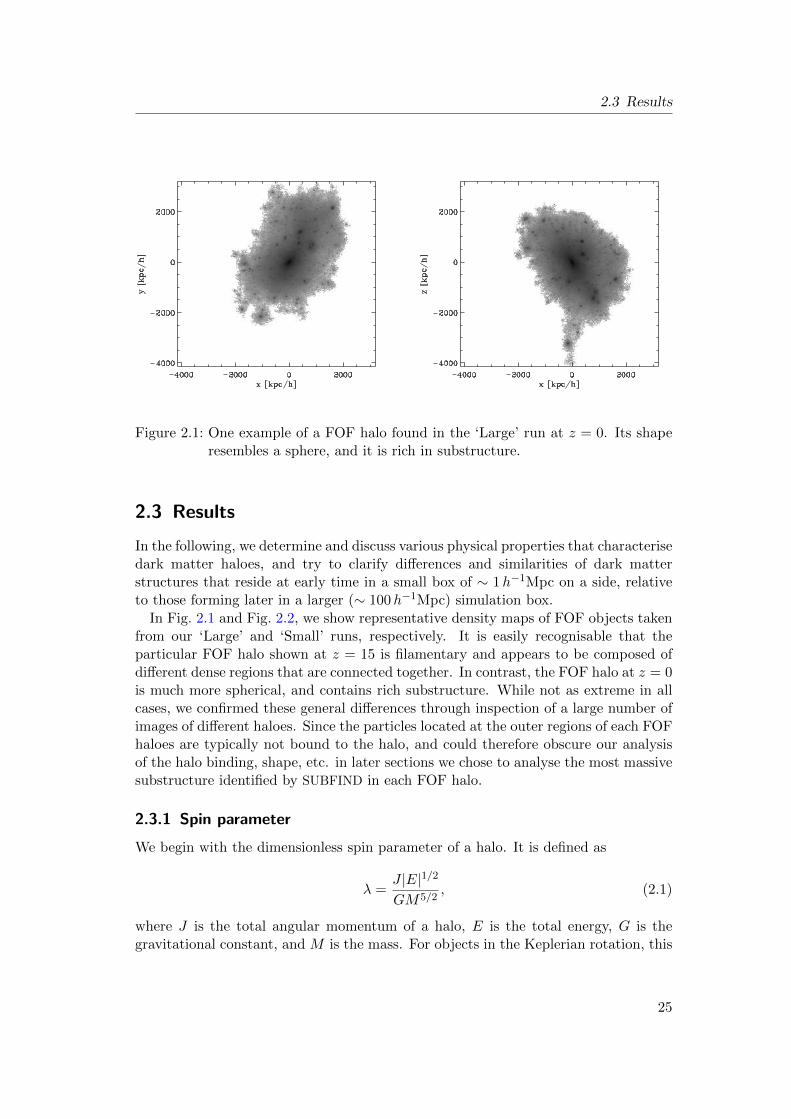
Figure 2.1: One example of a FOF halo found in the ‘Large’ run at z = 0. Its shaperesembles a sphere, and it is rich in substructure.
2.3 Results
In the following, we determine and discuss various physical properties that characterisedark matter haloes, and try to clarify differences and similarities of dark matterstructures that reside at early time in a small box of ∼ 1h−1Mpc on a side, relativeto those forming later in a larger (∼ 100h−1Mpc) simulation box.
In Fig. 2.1 and Fig. 2.2, we show representative density maps of FOF objects takenfrom our ‘Large’ and ‘Small’ runs, respectively. It is easily recognisable that theparticular FOF halo shown at z = 15 is filamentary and appears to be composed ofdifferent dense regions that are connected together. In contrast, the FOF halo at z = 0is much more spherical, and contains rich substructure. While not as extreme in allcases, we confirmed these general differences through inspection of a large number ofimages of different haloes. Since the particles located at the outer regions of each FOFhaloes are typically not bound to the halo, and could therefore obscure our analysisof the halo binding, shape, etc. in later sections we chose to analyse the most massivesubstructure identified by SUBFIND in each FOF halo.
2.3.1 Spin parameter
We begin with the dimensionless spin parameter of a halo. It is defined as
λ =J |E|1/2
GM5/2, (2.1)
where J is the total angular momentum of a halo, E is the total energy, G is thegravitational constant, and M is the mass. For objects in the Keplerian rotation, this
25

2 Small-scale structure formation
Figure 2.2: One example of a FOF halo found in the ‘Small’ run at z = 15. It has afilamentary shape.
value is of the order of unity. For our analysis of angular momentum, we includedonly haloes that have at least 1000 particles inside their main subhaloes, i.e. witha minimum mass of ∼ 104 M. The spin of dark matter haloes is a result of tidaltorques that they experience during their formation and subsequent evolution (White,1984).
We show the median, and 20%, 80% percentiles of this parameter in a series oflogarithmic mass bins in Fig. 2.3. We find that at all the redshifts we looked at, thespin parameter λ weakly depends on mass.
The distribution of λ is often fitted by a log-normal distribution (Warren et al.,1992):
p(λ) dλ =1√
2πσλexp
[− ln2(λ/λ)
2σ2λ
]dλ
λ. (2.2)
We obtained a log-normal fit to the spin distribution at z = 15 with parametersλ = 0.0262 and σλ = 0.495 (Fig. 2.4, top) for all haloes with at least 1000 particles.In other parts of this paper, lower limit of 100 particles is introduced such that lowermass haloes, which are not well-resolved, will be excluded from our analysis in thispaper (shape, virial ratios, formation times etc). We adopted a more demandingcriterion here, since the spin parameter is known to depend more strongly on howwell the dark matter haloes are resolved than other physical parameters (Davis andNatarajan 2010, see also Appendix A.3 of this paper). Jang-Condell and Hernquist(2001) found that the spin distribution follows a log-normal distribution at z = 10(with λ = 0.033, which is overplotted with a dashed-line in Fig. 2.4). The similarvalue in λ is a bit surprising, because although we model essentially the same volumein comoving space with slightly different redshift, the different mass resolutions in the
26

2.3 Results
two simulations mean that we resolve dark matter haloes in different mass ranges.This outcome is however consistent with findings from analytical works that predictthat λ has no strong dependence on the power spectrum (Heavens and Peacock, 1988).
Since we calculate spin parameter from substructure within FOF haloes, we do notsuffer from artificial high-end tail of spin distribution in Fig. 2.4 as in Bett et al. (2007),who analysed a simulation output produced with the same code as ours, GADGET-3,on a larger scale but chose to analyse FOF haloes.
Because the spin of a halo is a sum of slight differences in position and velocity space,it is sensitive to how well the halo is resolved. As such, our study qualifies as the mostprecise measurement of the spin parameter at z = 15 thus far. We expect that ourestimate of the spin parameter for subhaloes with mass > 104 h−1M (correspondingto > 103 particles) is correct within a factor of 2 at a 1σ level (Trenti et al., 2010).We obtain λ = 0.0247 and σλ = 0.486 for haloes in the mass range 105±0.2 h−1Mand λ = 0.0274 and σλ = 0.495 for haloes in the mass range 104±0.2 h−1M (Fig. 2.4,bottom). This is in contrast to the result of Davis and Natarajan (2009), wherethey find the more massive haloes to have systematically larger spin. This is a resultof different halo identification algorithms. The particles that lie in the surfaces ofdark matter haloes contribute little in terms of mass but much in terms of angularmomentum. Therefore, the actual value of spin parameter heavily depends on haloidentification methods employed. Comparison of Figs 2.3 and A.5 shows that theFOF gives a positive correlation between spin and halo mass, which is not presentwhen we employ the more conservative SUBFIND method.
In simulations with dark matter and gas, it has been found that the spin parametersof both components follow similar distributions (van den Bosch et al., 2002). As weaim to study the environmental conditions of first star formation, knowledge of λ isa key prerequisite. There is a recent work that estimates the Pop III initial massfunction (IMF) from the rotational velocity of haloes (de Souza et al., 2013). Hiranoet al. (2014) selected ∼ 100 haloes from multiple realisations of structure formationand resimulated many samples of Pop III star forming regions in a suite of two-dimensional radiation hydrodynamic simulations, ending up with a statistical studyof the final mass of a single protostar. Their spin distribution of the dark mattercomponent is centred on λ = 0.0495, considerably higher than the values found inmost pure dark matter simulations including ours. This is largely due to a selectioneffect and the positive mass-spin relationship of FOF haloes described earlier: theseauthors employed a standard FOF algorithm to extract the haloes, and focused on themore massive haloes in the simulation (i.e. those massive enough to have triggeredH2 cooling), which are likely to have higher spin.
2.3.2 Virial ratios
In this paper, we define the virial ratio as 2.0 × EK/EG, so that a value of unitycorresponds to virial equilibrium. The total kinetic energy EK is defined as
EK =1
2Σi miv
2i , (2.3)
27

2 Small-scale structure formation
Figure 2.3: Distribution of the dimensionless spin parameter λ in dark matter haloesof different mass at redshift z ∼ 25 (top panel), z ∼ 20 (middle panel),and z ∼ 15 (bottom panel). Crosses indicate the median value of λ, whilethe error bars indicate the 20th and 80th percentiles. The dashed verticallines represent lower mass limit of 1000 particles. We exclude any binsthat contained less than 10 samples. The same holds for Fig. 2.5.
28

2.3 Results
Figure 2.4: The top panel is the spin distribution for all haloes with ≥ 1000 particlesat z = 15. The bottom panel shows the spin distribution for haloes withina mass range of 105±0.2 h−1M (diamonds) and 104±0.2 h−1M (crosses).The symbols represent data from our simulations, and the lines indicatelog-normal fits. The vertical solid (dashed) lines represent λ for our (Jang-Condell and Hernquist 2001) simulation.
29

2 Small-scale structure formation
with velocity being defined relative to the centre-of-mass velocity of the halo through-out this paper. The gravitational potential energy EG is defined as
EG =1
2
∑i 6=j
Gmimj
rij. (2.4)
The sum is taken over all particles i and j that belong to the main subhalo in a specificFOF halo, with mi and mj being their mass, and rij their distance. This quantity isnumerically calculated by direct summation.
Fig. 2.5 shows the distribution of virial ratios for different dark matter haloes atredshifts z ∼ 25 (top), 20 (middle), 15 (bottom). We see that there is some variationin this quantity, but the median, and the 20%, 80% percentiles of the virial ratio arewell above unity for all mass ranges we have investigated, and thus the dark matterhaloes are not virialized but instead are usually perturbed. This has previously beennoted by Jang-Condell and Hernquist (2001) and Davis and Natarajan (2010), withrelatively low resolution at high redshifts, and also by, for example, Hetznecker andBurkert (2006) at lower redshifts, z < 3. It is also beneficial to compare results ofthe ‘Large’ box run with the ‘Small’ run. It is clear from Fig. A.3 that dark matterhaloes found in the larger simulation box at z = 0 have systematically lower virialratios, and are thus closer to virial equilibrium than those at z = 15.
The median value of the virial ratio in Fig. 2.5 increases with increasing halo mass.The median value of a given mass bin does not evolve considerably over a rangeof redshift, in contrast to Hetznecker and Burkert (2006), who have found that thevirial ratio decreases monotonically with redshift between z = 3 and z = 0. Thesedifferences reflect the different dynamical states of dark matter mini-haloes at z ≥ 15and more massive systems at z < 3.
Our results show that dark matter haloes at z ∼ 15 cannot be considered to typicallyrepresent isolated systems undergoing collapse (see also discussion in Section 2.3.6).The excess kinetic energy of the dark matter haloes, if shared by their gas component,could influence the star formation taking place because the properties of the turbulencein the interstellar medium strongly influence the star formation process within them(Clark et al. 2011a, Prieto et al. 2012). Distinguishing relaxed haloes from unrelaxedhaloes is not a straight-forward task, and needs to be based on complex criteria thatinvolve, for example, virial ratios and the fraction of mass in substructures (Netoet al., 2007). Our simple definition of virial ratio should however already give a usefulproxy for the dynamical state of a halo.
2.3.3 Mass function
We now compare the halo mass distribution with predictions of analytical models.Let ∆n be the number density of objects with mass (FOF mass found for our groupsor mass of main subhalo in our group) within a logarithmic bin, and ∆ logM belogM2/M1 where M2/M1 is the ratio of upper and lower values for each mass bin(constant). In Fig. 2.6, ∆n
∆ logM is plotted against the median value in each massbin along with Poisson error bars (error bars are omitted for subhalo data for easy
30

2.3 Results
Figure 2.5: Distribution of the virial ratio in dark matter haloes of different mass atredshift z ∼ 25 (top panel), z ∼ 20 (middle panel), and z ∼ 15 (bottompanel). The virial ratio is defined such that it tends to unity at virialequilibrium. Crosses indicate the median value of the virial ratio, whilethe error bars indicate the 20th and 80th percentiles. The mass bins arespaced logarithmically, and symbols are only plotted for bins containingat least 10 dark matter haloes.
31

2 Small-scale structure formation
Figure 2.6: Mass function of dark matter haloes at z = 15 (diamond symbols representnumber counts for FOF haloes, when crosses denote those for the mainsubhalo in a FOF halo). The Press-Schechter (Press and Schechter, 1974)and Sheth-Tormen functions (Sheth and Tormen, 1999) are over-plotted.
recognition). The analytical Press-Schechter (Press and Schechter, 1974) and Sheth-Tormen models (Sheth and Tormen, 1999) are plotted with continuous and dottedlines, respectively. The Press-Schechter function underestimates the number of haloesin the high mass range, whereas the Sheth-Tormen function gives a good fit to thesimulated FOF data over a broad range of masses including the high-mass end. Sincesubhaloes contain only part of mass of its host FOF haloes and therefore some of thehaloes that belonged to a particular mass bin is shifted to neighbouring lower massbin, number density of subhaloes in a given mass bin is systematically smaller thanFOF haloes. Overall, we find that these analytical fitting formulae reproduce notonly the statistics of dark matter haloes with mass 107 h−1M as previously known(Ishiyama et al., 2013) at z = 0, but they also describe less massive haloes obtainedfrom our simulations, such as those as small as 103 h−1M at z = 15.
2.3.4 Formation time
The linear power spectrum of density perturbations at z = 0 for the cosmologicalparameters we adopt in our work is plotted in Fig. 2.7, where the dark blue line showthe critical slope of −3. In this section, we express the slope of the power spectrumby p. Therefore, P (k) ∝ kp, where the slope p changes as a function of wavenumberk. For the linear power spectrum shown in Fig. 2.7, p = −2.37,−2.62,−2.74,−2.80at k = 1, 10, 100, 1000h Mpc−1.
The power spectrum increases at very low wavenumbers, then turns over and startsto decrease again, approaching power law with p ' −3 at high wavenumbers. Forthe mass scales extensively studied by earlier works, Mhalo ∼ 1012 h−1M, the slopeis substantially shallower compared to a mass scale of Mhalo ∼ 106 h−1M where
32

2.3 Results
Figure 2.7: The linearly extrapolated power spectrum of dark matter at z = 0 for thecosmological parameters we adopt. The critical slope of k−3 is shown withdark blue line.
the slope is close to the critical value of p = −3. It is critical in the sense that thenon-dimensional power,
∆2(k) =k3P (k)
2π2(2.5)
becomes independent of wavenumber k. ∆2(k) represents the amount of perturbationsin a logarithmic bin in k. For p > −3, ∆2(k) is a monotonically increasing functionof k. Therefore, given p > −3, for a fixed time, there is more power in small scales(large k) than in large scales (small k). Thus, small gravitational structures form firstin such regimes (explicitly shown in Fig. 1 in Harker et al. 2006). In contrast, forp = −3, ∆2(k) is independent of wavenumber k, thus the dark matter structures ofvarious mass collapse simultaneously and in a non-hierarchical fashion. We now showthis explicitly using our high-resolution simulation.
Adopting the methods described in Section 2.2.1, we identified the formation timeof each FOF halo. In Fig. 2.8, we divide dark matter haloes in various mass bins andplot the median, and 20%, 80% values of formation time in each mass bin. We findthat in the mass range we are interested in, massive dark matter haloes and smallhaloes form simultaneously (this is only true statistically, because there is a dispersionof ∼ 10 Myr in the formation time in a given mass bin). This is quite different fromthe more massive regime, where less massive haloes form first (Harker et al. 2006, alsosee results of the ‘Large’ run in Fig. A.2). This implies that the formation processesof dark matter mini-haloes found at high redshift in a simulation box of 1h−1Mpcdiffer substantially from those found at much higher halo masses in larger boxes.
33

2 Small-scale structure formation
Figure 2.8: Formation time of dark matter haloes as a function of their mass. Median,20 %, and 80 % values in each mass bin are plotted. Haloes that differin mass by ∼ four orders of magnitude form simultaneously. This is quitedifferent from the formation time for more massive systems at z = 0.Compare with Fig. A.2.
2.3.5 Halo shape
Often the high-density regions found in collisionless N -body simulations are not ex-actly spherically symmetric, as opposed to the assumption which is made to derivePress-Schechter mass function for example. Modelling dark matter haloes as ellip-soids and measuring their three axes provide a way to quantify the shape of thesehaloes and how much it differs from the spherical collapse model. Moreover, there areseveral different kinds of approaches made observationally to estimate halo shapes inthe local universe: First, there are ways to measure dark matter distribution by weaklensing using X-ray clusters (Oguri et al., 2010). Secondly, there are also attempts todetermine dark matter halo shapes for galaxies statistically using surveys (Hoekstraet al., 2004). Lastly, there are also efforts made to derive the gravitational potentialof our Galaxy by using the kinematics of tidal tails of the Sagittarius dwarf spheroidalgalaxy (Law et al., 2009). The less massive haloes found in our study are influencedby a much shorter wavelength portion of the ΛCDM power spectrum than the haloesexamined in these observational studies, and it is therefore interesting to see whetherthere is any systematic difference in the shapes of these mini-haloes.
We define a second moment tensor of the halo shape as:
Iij =∑n
xixj , (2.6)
where xi (i = 1, 2, 3 corresponding to x, y, and z coordinates) is the particle positionwith respect to the centre of the halo, which we define as the position of the particlewith the lowest potential energy. The same form of the shape matrix was adopted
34

2.3 Results
Figure 2.9: Median of sphericity s and triaxiality T in different mass bins for darkmatter haloes at z = 15. The sphericity and triaxiality are defined byequations (2.10) and (2.11), respectively.
in the earlier studies of Jang-Condell and Hernquist (2001) and Maccio et al. (2008).We note that sometimes Iij is defined as
∑n xixj/r
′2, i.e. with a 1/r′2 normalisationfactor (Moore et al. 2004, Allgood et al. 2006). But we here adopt the former, morewidely used formulation.
The sum is taken over all the particles that belong to the main subhalo in a FOFhalo. After evaluating the inertia tensor, we compute its eigenvalues I1, I2, and I3,which are the three principal moments of inertia of the halo, and which satisfy therelationship I1 ≥ I2 ≥ I3. The lengths of the axes a, b, and c associated with theprincipal moments of inertia are given by
a =√
(5 I1)/Np, (2.7)
b =√
(5 I2)/Np, (2.8)
c =√
(5 I3)/Np, (2.9)
where Np is the number of particles summed up in equation (2.6). The sphericity ofthe halo is then defined as
s = c/a. (2.10)
From the above formulation, it should be clear that a spherically symmetric halo hass = 1. The triaxiality of the halo is defined as
T = (a2 − b2)/(a2 − c2). (2.11)
By definition, an oblate halo (a = b > c) has T = 0, and a prolate halo (a > b = c)has T = 1.
35

2 Small-scale structure formation
Black solid lines in the different rows in Fig. 2.10 show the distribution of sphericitys for different mass ranges (namely haloes with mass 104±0.2 h−1M, 105±0.2 h−1M,and 106±0.2 h−1M). We find that the distribution of s based on all haloes has apeak at 0.4 − 0.45, which is smaller than the value typically found for more massivehaloes at lower redshifts. For example, Allgood et al. (2006) and Maccio et al. (2008)investigated haloes with masses ∼ 1012 h−1M to 1015 h−1M and found almost nohaloes with s < 0.4. This could be due to more frequent mergers at z = 15 comparedto z = 0.
If we compare the distribution function of s and T , 105 M haloes are more likelythan 104 M haloes to have lower values of sphericity s and higher values of triaxialityT . This tendency of more massive haloes having small s and larger T , that has beenobserved elsewhere (Allgood et al. 2006, Maccio et al. 2008), is even clearer in Fig. 2.9,in which we show median values of s and T as a function of halo mass. ComparingFig. 2.9 with Fig. A.1, we find that haloes found at z = 0 are systematically morespherical and only moderately more prolate compared to haloes at z = 15.
Fig. 2.10 also shows that for all the three different mass ranges studied here, alarge fraction of haloes are prolate (T ∼ 1). This is similar as found in previousstudies that focused on haloes forming in different regimes (e.g. more massive haloes,Dubinski and Carlberg 1991, Warren et al. 1992). This is most likely because darkmatter haloes of various mass scales form from filamentary structures. However, wefind a significant disagreement with de Souza et al. (2013), who worked on similarmass ranges and practically the same redshift, but with hydrodynamical simulations.Their dark matter haloes with mass ∼ 105 M at 11 < z < 16 have s ∼ 0.3 and morethan 90% have T . 0.4, whereas the dark matter haloes with mass ∼ 105 h−1M atz = 15 in our simulations have medians s ∼ 0.4 and T ∼ 0.85. We note that de Souzaet al. (2013) adopt a definition of Iij equivalent to ours. The difference in shape couldbe due either to the inclusion of gas cooling or to a very different mass resolution. Weresolve substructures inside dark matter haloes with mass ∼ 105 h−1M with ∼ 104
particles, whereas de Souza et al. (2013) resolve haloes with the same mass with only∼ 200 particles. We speculate that the inclusion of gas makes a bigger difference thanthe mass resolution, however, since our convergence study shows that even with arelatively small particle number of 200 particles or so, the errors in the axial ratios(b/a, c/a) remain within 10% (see Table A.2).
Histograms with different colour in Fig. 2.10 represent halo shape distributions forhaloes with different values of the spin parameter. We sorted dark matter haloes ineach mass range into percentiles according to their spin. If we denote the 33% and67% percentile values of the spin parameter in each mass range as λ1/3 and λ2/3, wehave plotted the probability distribution of halo shapes for three different kinds ofhalo selections: all the haloes in a certain mass range, only haloes with λ > λ2/3,and only haloes with λ < λ1/3. We found that, in all the mass ranges we looked at,dark matter haloes with high spin are less spherical and more highly prolate, a trendalready confirmed in lower redshift dark matter haloes by previous works (Bett et al.,2007). Davis and Natarajan (2010), who used different methods to identify haloes andestimate their shapes, also found similar trends for high-redshift dark matter haloeswith relatively low resolution. This widely observed correlation could occur because
36

2.3 Results
haloes that experienced strong gravitational forces during their formation are likelyto have high spin and an aspherical shape.
In short, using the highest-resolution simulation to date for resolving a large sampleof substructure inside dark matter mini-haloes of mass > 103 M, we have demon-strated that dark matter mini-haloes we find in our simulations at z ∼ 15 havequalitatively many similarities with dark matter haloes found at z <∼ 6 regardingtheir shape.
2.3.6 Correlation between formation time and virial ratio / formationtime and halo shape
Many authors have studied the effect of the mass accretion history on the concen-tration and density profile of dark matter haloes (Bullock et al. 2001, Wechsler et al.2002, Tasitsiomi et al. 2004). Much less work has been done on the relationship be-tween formation time and other halo properties. For dark matter haloes found inmass scales capable of hosting Pop III star formation, we show for the first time thatthere is a direct connection between the shape of a halo, its dynamical state, or itsspin and its formation time. This could provide interesting clues on the formationprocesses of dark matter haloes.
We sorted the dark matter haloes in different mass bins into three groups accordingto their formation time. In Fig. 2.11, we show that the haloes that formed later (younghaloes) have higher values of the virial ratio, while in Figs 2.12 and 2.13, we showthat haloes that formed later (young haloes) have smaller sphericities and larger spinparameters. This is because haloes of a given mass that formed later accumulatedtheir mass recently, and thus had no time for relaxation.
To clarify this point, let us make comparison of relevant time-scales. The Hubbletime, tH = a/a is ∼ 300 Myr at z = 15. If we estimate the relaxation time trelax of darkmatter haloes by trelax = 1√
Gρ= 1√
G200ρcrit(z=15), trelax ∼ 60 Myr at z = 15 (< tH,
as expected). The old haloes analysed here typically formed at around z = 18 − 20whereas the young haloes formed at z < 16. Thus the former typically had morethan ∆t(z = 18, z = 15) ∼ 80 Myr (> trelax) while the latter had less than ∆t(z =16, z = 15) ∼ 45 Myr (< trelax) since the time of formation. This could account for thedifferences in physical properties we observe when we stop our simulation at z = 15.
In fact, Hetznecker and Burkert (2006) have demonstrated that major mergersincrease the value of the spin parameter and the virial ratio. Allgood et al. (2006)have also found that haloes forming earlier (old haloes) are more spherical. Theyhave also shown that the dependence on formation time is weaker for higher masshaloes, at least in their simulation box. The different methods adopted to calculatehalo shape and formation time preclude a direct comparison, but the high-mass endof Fig. 2.12 clearly shows similar trends.
Our results confirm that the formation epoch of dark matter haloes influences globalparameters such as shape, virial ratio, and spin. Each dark matter halo has a differentevolution history. Furthermore, even the dark matter haloes that have similar massaccretion histories could have accreted their mass from different spatial locations orthrough different channels. A single global parameter such as formation time is not
37

2 Small-scale structure formation
Figure 2.10: Sphericity s and triaxiality T for haloes with mass 104±0.2 h−1M,105±0.2 h−1M, and 106±0.2 h−1M at z = 15. Different lines representdistributions for different groups in each mass range. (Blue dotted linescorrespond to haloes with λ < λ1/3, green dash-dotted lines correspondto haloes with λ > λ2/3, and black solid lines correspond to all subhaloes
in that mass range.)
38

2.3 Results
Figure 2.11: Relation between formation time and virial ratios. We grouped the haloesin each mass bin into three groups. Early one-third (old haloes), middleone-third (intermediate haloes), and late one-third (young haloes). Weplot the median values for early (crosses) and late (diamonds) thirds.The error bars indicate 20th and 80th percentile values for each group.(Error bars are plotted in solid lines for haloes forming earlier, and indotted lines for haloes forming later. For easy reference, haloes forminglater are slightly offset in mass.) We found that haloes that formed later(young haloes) have higher virial ratios on average due to lack of timefor relaxation.
enough to account for this, and the scatter in Figs 2.11 and 2.12 could be due tovariations in the processes that let haloes accumulate their mass.
2.3.7 Correlation function
The two-point correlation function calculated from N -body simulations is a usefulquantity, since it can be compared directly with galaxy clustering data (Springel et al.,2005). We perform a similar analysis to clarify the properties of the mini-haloes wefind at z = 15. Gao et al. (2005) have demonstrated that haloes that assembled earlierare more strongly clustered, casting doubt on an assumption made in excursion-settheory (Bond et al., 1991), namely that halo properties depend only on mass and areindependent of environment.
Here we study the clustering of haloes with different spins. In order to quantify theclustering between dark matter mini-haloes, we make two kinds of catalogues of darkmatter haloes: a simulated halo catalogue and a random catalogue. The simulatedhalo catalogue is a list of positions of haloes obtained from our simulation. Therandom catalogue is a list of random points distributed in a box that is equal in sizeto our simulation box. We measure the two-point correlation function ξ(r) following
39

2 Small-scale structure formation
Figure 2.12: Relation between formation time and sphericity. We grouped the haloesin each mass bin into three groups. We plot the median values with errorbars for early (crosses) and late (diamonds) thirds as in Fig. 2.11. Wefound that haloes that formed later (young haloes) are less spherical dueto recent mass accumulation.
Figure 2.13: Relation between formation time and spin parameter. We grouped thehaloes in each mass bin into three groups. We plot the median values witherror bars for early (crosses) and late (diamonds) thirds as in Fig. 2.11.We found that haloes that formed later (young haloes) have higher valuesof spin parameter due to recent mass accumulation. The dashed verticallines represent lower mass limit of 1000 particles.
40

2.4 Conclusions
Hamilton (1993),
ξ(r) =DD(r)RR(r)
RD(r)2− 1, (2.12)
where DD(r), RD(r), RR(r) stand for, respectively, the number of pairs with separa-tion r in the simulated halo catalogue (halo-halo pairs), the simulated halo catalogueand random catalogue (halo-random point pairs), and just the random catalogue(random point-random point pairs). The statistical errors are estimated throughRR(r)
√DD(r)/RD(r)2.
The two-point correlation functions for haloes in the mass bin 105±0.2 M and104±0.2 M are depicted in Fig. 2.14 as a function of separation in units of comovingh−1kpc. As in Section 2.3.5, we sorted dark matter haloes in both mass ranges intothree subsets according to their spin. We found that haloes with high spin are moreclustered, which is well-known in large-scale simulations (Bett et al. 2007, Gao andWhite 2007), but was only investigated with relatively low resolution in much smallerscales (Davis and Natarajan 2009). This suggests that haloes that form in a clusteredenvironment are more likely to experience tidal forces from neighbouring overdenseregions, and therefore tend to have larger spin parameters.
2.4 Conclusions
In this paper, we have performed a high-resolution numerical simulation of structureformation up to the high redshift z = 15, inside a simulation box of side-length1h−1Mpc. Exploiting our good statistics and resolution, we made high precisionmeasurements for a variety of global physical parameters of haloes and demonstratedcorrelations between some of these properties. We clarified the characteristics of darkmatter mini-haloes by comparing the results of our high-resolution simulation withworks found in the literature on more massive haloes and at lower redshift (z < 6),and with results from our own moderate-resolution complementary simulation withina cubic region of 100h−1Mpc on a side that we evolved until z = 0. Our main findingsare as follows.
1. Dark matter haloes found in our simulations have a distribution of spin pa-rameters that is well fitted by a log-normal function around λ = 0.0262, withdispersion σλ = 0.495. This value for λ is similar to the value ∼ 0.03 obtainedby studying more massive objects at z ∼ 0 (e.g. galaxy clusters). The dimen-sionless spin parameter λ is somewhat sensitive to resolution, and hence ourmeasurement of this quantity is by far the most accurate thus far for the massscales investigated in this work.
2. We have shown explicitly from output of our simulations and merger trees con-structed from them that the formation time of dark matter haloes, defined asthe time at which the most massive substructure in a FOF halo reaches half ofits final mass, only weakly depends on halo mass over about four orders of mag-nitude (e.g. mass scales of ∼ 103–107 M). At larger mass scales, structures areknown to form in a hierarchical fashion (formation redshift is a monotonically
41

2 Small-scale structure formation
Figure 2.14: Two-point correlation function for dark matter haloes in the mass range105±0.2 h−1M and 104±0.2 h−1M. Distance is in units of comovingh−1kpc. We have reproduced the trend seen in previous works that highspin haloes are more highly correlated than low spin haloes.
42

2.4 Conclusions
decreasing function of halo mass). But on the mass scales investigated here, thisat least partially breaks down. The weak dependence of the formation time onmass is a result of the slope of the power spectrum of density perturbations atthis scale, where it becomes close to the critical value of −3 for which all massperturbations are expected to collapse simultaneously. The scatter in formationtime is ∼ 10 Myr.
3. The shapes of haloes are much less spherical and more highly prolate than haloesfound at z ∼ 0. The most frequent value of the sphericity parameter lies between0.4 and 0.45. This could be due to more frequent mergers at high redshift. Themajority of haloes have triaxiality parameter > 0.9. More massive haloes aremore likely to be slightly less spherical and slightly more filamentary (prolate).
4. We have also investigated the relationship between formation time and haloproperties such as shape, virial ratios, and spin which was not studied previouslyfor the scales examined here. On average, haloes that formed more recently(young haloes) have higher values of the virial ratio, are less spherical, and havehigher values of spin when observed at z = 15. This can be understood becausethe time passed between the formation of these young haloes and the end of thesimulation is less than the relaxation time, trelax ∼ 60 Myr, of these haloes.
5. Although not expected from excursion set theory, we find that haloes with highspin are more strongly clustered, where clustering is quantified by the two-point correlation function of the positions of different dark matter haloes. Thiscould mean that haloes born in clustered environments experience stronger tidaltorques during their formation.
In this study, we have investigated broad aspects of dark matter haloes at high-redshift and found many similarities with their low-redshift counterparts. Our findingscould have important implications for the baryonic component of dark matter haloesfound at high-redshift. Our results on the correlation between formation time andvirial ratio/shape imply that the gas component inside each dark matter halo couldevolve differently depending on accretion history and the actual dynamics of accretion.
Potential caveats of our work include starting redshift of our simulations and ex-clusion of surface terms in estimating the virial ratios. We will briefly discuss themin the following paragraphs.
Reed et al. (2007) show that an initial redshift of 139 should be safe for studyingobjects at z ' 7-15. Since suppression of high sigma density peaks that result fromuse of first order perturbation theory and low starting redshift is known to be strongerat high redshift (Crocce et al., 2006), it is possible that we are missing some of thedark matter haloes at the high mass end, especially when studying properties such asspin parameter of them at z ∼ 25. Due to this suppression effect, we could be under-estimating the two-point correlation function and formation time of dark matter haloesas well.
It is pointed out in recent literature (Ballesteros-Paredes 2006, Davis et al. 2011)that the surface terms in virial equations are in general not negligible. Once these
43

2 Small-scale structure formation
terms are taken into account, dark matter haloes tend to have less excess kineticenergy. However, Davis et al. (2011) show that even after correcting for the surfaceterms, dark matter haloes have virial ratios that are greater than one and that increasewith increasing redshift. Therefore, although we would expect a systematic decrease inthe absolute values of virial ratios once we include the surface terms, our main resultsregarding the dependence of the virial ratio on halo mass and formation redshift shouldbe sound.
In a future study, it would be interesting to directly follow the star formation takingplace in different dark matter mini-haloes by means of hydrodynamical simulations,and to clarify how the global dark matter properties investigated here are connectedto the properties of the resulting Pop III stars.
Acknowledgements
M.S. acknowledges computing time from Hochstleistungs Rechenzentrum Nord (HLRN)under project hhp00022 and financial support from the Heidelberg Graduate Schoolof Fundamental Physics (HGSFP). R.S.K. acknowledges support from the EuropeanResearch Council under the European Communities Seventh Framework Programme(FP7/2007-2013) via the ERC Advanced Grant“STARLIGHT: Formation of the FirstStars” (project number 339177). M.S. and R.S.K. thank for funding from the Baden-Wurttemberg Foundation in the program Internationale Spitzenforschung (contractresearch grant P-LS-SPII/18). M.S. wishes to thank Matthias Bartelmann for clari-fying some of the basic concepts in structure formation.
44

3 Improving the advection of chemicalspecies in the Arepo code
In this chapter, we first describe the basic principles of the AREPO code and laterdemonstrate some minor modifications we have made to the code.
3.1 Numerical methods
AREPO is a hybrid code that uses an unstructured mesh (i.e. Voronoi tessellation)to deal with the known shortcomings of previous Eulerian and Lagrangian methodsfor solving hydrodynamics. While it uses a Riemann solver to solve equations thatgovern hydrodynamics and there are mass flows between cell surfaces, it is particle-like in that the cells themselves are allowed to move. Thus it does not suffer from thelack of fluid instabilities or the lack of mixing at surfaces between fluids of differentdensity, which results from the use of a smoothing kernel, or have difficulty treatingshocks as traditional particle-based codes. It can also deal with fluids with large bulkmotions without introducing errors, unlike traditional mesh-based codes. The detailedprocedures that the simulation code follows is described in the chart in Fig. 3.1 (takenfrom Fig. 18 of Springel 2010), so we summarise only the most important aspects inthis section.
From a purely Eulerian point of view, the fundamental equations of hydrodynamicsare reduced to following the evolution of the vector
U =
ρρvρe
=
ρρv
ρu+ 12ρ|v|
2
, (3.1)
where ρ is the mass density, v is the velocity, u is the specific internal energy, and eis the specific total energy. This vector evolves according to a continuity equation ofthe form
∂U
∂t+∇ · F = 0, (3.2)
where the flux function F is given by
F (U) =
ρvρvvT + Pρ(ρe+ P )v
. (3.3)
45

3 Improving the Arepo code
In understanding how this moving-mesh code works, it is important to know thatthere are two kinds of variables defined for each cell: ‘primitive’ and ‘conserved’.Primitive quantities here include the density ρ, the velocity v, and the pressure P =(γ − 1)ρu (ρ, v, P ). These quantities determine the state of each cell, and theyare used for solving the Riemann problem. Conserved quantities, namely, the mass,the momentum, and the energy, are obtained by integrating vector U (defined inequation (3.1)) over the volume of the cell. By solving the Riemann problem at cellfaces, we can calculate the change in conserved quantities. Simply put, the followingprocedures are what is taking place at every timestep to follow the evolution of vectorU inside the code (according to a paragraph in section 3 in Springel 2010, notationssimilar):
1. Construct a new Voronoi tessellation based on the current coordinates of themesh-generation points. From this, conserved quantities for each cell can becalculated.
2. From conserved quantities calculate the primitive quantities (ρ, v, P ) for eachcell.
3. Estimate the gradients of the primitive quantities (ρ, v, P ).
4. Assign velocities to the mesh-generating points.
5. Use the Courant condition to determine appropriate timestep (divide radius ofthe cell by its sound speed to obtain a timescale).
6. For each surface between cells, compute the flux from the left and the rightstates of the face (solve the Riemann problem).
7. For each cell, update the conserved quantities.
8. Move the mesh-generating points with their assigned velocities for this timestep.
When we started working with the subroutine to solve primordial chemical reac-tions in AREPO, the code could already advect the species when the cells moved. Thisgave an approximately correct solution, but it did not account for the flux of speciesfrom cell to cell. Therefore we decided to make modifications to include this effect.Of course, already in the main body of AREPO, the fundamental quantities such asthe mass, the momentum and the energy are properly calculated with fluxes fromneighbouring cells taken into account (as described in the above procedure), but theabundance of chemical species that is transported to the neighbouring cell with theflow was neglected in the original setup. We describe here the details of the modi-fications we made to the code to account for this effect. Technically, the primordialchemical reactions are calculated inside a subroutine which is called at the end of eachloop, after the second gravitational half kick is applied (Fig. 3.1). In the next sec-tion, we describe two technical (numerical) difficulties we have experienced, and thecode fixes to get around such problems. These are both related to the computation offluxes between neighbouring cells (step (6), (7) in the above diagram). The primordial
46

3.1 Numerical methods
Figure 3.1: Flow chart of the simulation code: Figure taken from Springel (2010)
chemical network solver used here includes H2,H+,D+,HD,He+,He++,H,D,He, e−.
Inside the code, two quantities relevant for each chemical species are stored. The in-tensive variable, ‘abundances’, and the extensive value, ‘total amount of each chemicalspecies (= cell mass × abundance of that species)’ (hereafter, ‘conserved abundances’for clarity). It is customary in the field of simulations with chemistry to normalise the‘abundance’ of each chemical species by the number of protons. For example, in caseof gas that consist purely of hydrogen atom (H) and helium atom (He), the abundanceis fH = 0.76 and fHe = (1 − 0.76)/4 = 0.06, respectively. By using this definition ofabundances, the ‘conserved abundances’ inside each cell will be described simply bymifx,i, where mi is the mass of cell i, and fx,i is the abundance of chemical species xin cell i.
Technically, solving fluid equations numerically and the chemical reactions that arecoupled to them simultaneously is a challenging task, since chemical reactions usuallyproceed much more quickly than the motion of the fluid. We briefly describe themethods adopted in our work here. If we represent the mass density of the chemicalspecies i by ρi, the continuity equation for this species reads
47
3 Improving the Arepo code
∂ρi∂t
+∇ · (ρiv) = Ci −Di, (3.4)
where Ci and Di represent the source and sink terms of chemical species i due tochemical reactions. Timescales associated with source/sink terms are shorter than thethe advection timescale. Therefore, when we solve the set of equations numerically,we use operator splitting, and solve the continuity equation without source or sinkterms (equation (3.5)) separately from chemical rate equations (equation (3.6)).
∂ρi∂t
+∇ · (ρiv) = 0 (3.5)
dρidt
= Ci −Di (3.6)
After operator splitting, chemical rate equations can be solved by subcycling, withstandard ordinary differential equation (ODE) solvers, as described for example inGreif et al. (2011, 2012). Technical challenges in this project involve the estimate ofabundances of chemical species at cell surfaces and the estimate of fluxes between thecells, as we describe in the next section.
3.2 Technical challenges
In short, we have used the gradient estimation of scalar values inside the code, andestimated the chemical abundances of each species at the surface of each cell. This isdone by adding two correction terms to the chemical abundances at the cell centre.One term is due to the spatial gradient and the disposition between cell face and cellcentre (spatial-component). The other term accounts for the fact that each cell facehave velocity and represents spatial gradient of chemical species times the distancethe cell face travel in half the relevant timestep (time-component). Since the numberof hydrogen atoms, helium atoms, and deuterium atoms should be conserved, wenormalise these values at the surface of each cell, which is a recommended methodwhen treating advection of multi-fluid flows (Plewa and Muller, 1999). Technically,this is done by multiplying the abundance of each chemical species by the correctionfactor, 1/Σjfj where index j runs through all the chemical species in the chemicalnetwork that contain element H, He, and D respectively. Note that for chemicalspecies HD, normalisation is done according to D (not H). In each cycle, when flowbetween the cell faces are allowed (note Fig. 3.1), the chemical abundances is alsotransported with the flow. This is essential in order to conserve elemental abundancesin the simulation domain.
One technical difficulty was that the estimate of the chemical abundances at the cellsurface can become negative due to moving-mesh nature of AREPO, especially whenthe chemical abundances of two neighbouring cells differ drastically. This could bethe case since the sum of extrapolation due to spatial gradient and extrapolation dueto velocity at the cell surface can become negative. Consider for example a spherical
48

3.3 Results
region abundant in chemical species i that has some bulk velocity in the direction ofthe arrow (Fig. 3.2), and this species has a very small abundance outside of this sphere.The shaded boundary regions inside the sphere close to the left ridge gets a negativecontribution from both the fact that it is closer to chemically-poor outside regions, andalso from the fact that such regions are approaching. The same problems is presentalso for adiabatic indexes as well in the opposite side of the ridge if the sphericalregions is fully molecular and the outside regions is fully atomic, since adiabatic indexchanges from 7
5 inside of the sphere, to 53 outside of the sphere in an abrupt way. At
the cell interfaces the estimate of the chemical abundances is forced to be 0 (adiabaticindex is forced to be 7
5) inside the code in such a case. This can be a problem forvery artificial test cases such as the ones described in Section 3.3.1. However, in realapplications of the code, we did not experience cases where this becomes a problem,since in a primordial gas that we studied with this code, the abundance of H2 is agradually increasing function of the density of the gas, and we do not have very sharpchanges in chemical abundances. Usually, in the real applications of this code, theproblem we describe in the next paragraph was more common.
Another technical difficulty arises when there is mass outflow from a cell that hasabundance of chemical species i to a cell that contains a much higher abundance ofthat species. Consider for example the case depicted in Fig. 3.3. In the two cellsillustrated, the left cell has a low abundance of chemical species i, when the right cellis much more abundant in this species. At the left side of the interfaces between twocells (L), the estimate of chemical abundance is larger than inside the left cell (cellA), since the chemical abundance is increasing as you approach cell B. The amount ofchemical species transported from the left cell to the right cell is determined by thisestimated value at the left (upwind) side of the interface multiplied by the mass flowcalculated from Riemann solvers. In such a case, the cell attempts to advect more ofthat species than is present inside the cell. One simple solution would be to simplyabandon extrapolation at the cell faces and simply use the abundance at the cell centrewhen calculating flux of chemical species (Volker Springel, private communication).In our implementation, rather than using this lower-order method, after the fluxis transported between cell faces, it is checked whether ‘conserved abundances’ ofchemical species inside a cell becomes negative, and some small yet positive floorvalue is enforced if this condition is not satisfied.
3.3 Results
We have performed different kinds of test calculations to test our implementation. Thefirst series of simulations test the behaviour of AREPO cells in a simple setup, namely,when the gas density is initially uniform, and only the chemical composition is different(fully molecular inside a sphere, and fully atomic outside). For simplicity, this firstseries of simulations do not include cooling due to chemical species or cooling/heatingdue to chemical reactions. We try with two different initial conditions in this setup.The second series of simulations is a more realistic application of the code to model acollapsing gas cloud in two different setups: an isolated rotating gas cloud and a gas
49

3 Improving the Arepo code
abundance of
chemical species
Figure 3.2: A simple example to illustrate a case where the estimate for chemicalabundances/adiabatic index can be negative. The red sphere is abundantin chemical species i and is fully molecular. Everywhere outside of thesphere, there is very small abundance of this species and it is fully atomic.The sphere has a bulk velocity in the direction of the arrow. The shadedregion in the red circle in the figure can get negative values.
cloud collapsing in a cosmological simulation. In total, we experiment with four kindsof test problems in this section.
3.3.1 Idealised tests
In this section, we test our implementation with two sets of test problems. Both casesinvolve a spherical region where hydrogen is molecular, and outside of this sphere,hydrogen is fully atomic. The main differences are for ‘bulk velocity’ set up, all thecells in the simulation box have a bulk velocity, whereas for ‘turbulent velocity’ setup, the velocity varies according to the location of the cell. The size of the simulationdomain is also different for the two setups. On-the-fly refinement is not enabled foreither of the two tests.
For the ‘bulk velocity’ setup, we placed a spherical region of fully molecular hydro-gen inside a periodic box of uniform density, which is originally in pressure equilibriumwith the fully atomic gas outside. The box size is 30.85 [1017cm], with 100 M in-side. We have turned off cooling due to chemical species but not the primordialchemical network itself. All the gas cells in the box have bulk velocity in the positivex direction. We have compared abundance of molecular hydrogen for two cases withand without advection of chemical species. Note that the run with advection has105 particles when the run without advection has 106 particles. We see that for therun with advection, the H2 molecules are actually advected in the surrounding cell
50

3.3 Results
abundace of
chemical species
L RA B
L
R
Figure 3.3: A simple example to illustrate a case where the total amount of chemicalspecies can be negative after flux exchange. Cell A has a smaller abun-dance of chemical species i, when the neighbouring cell (cell B) has a muchlarger abundance of the same species. Assume there is mass flux into cellB from cell A. L and R represent the left side and the right side of a cellface described here. The blue triangles represent the estimated abundanceof some chemical species according to gradient of chemical abundances atcell faces L and R, respectively. Note that the estimated abundance atL, which is used to calculate the amount of chemical species transportedfrom cell A to cell B, is larger than the abundance in the centre of cell A,which is represented by the left lower plateau in the figure.
51

3 Improving the Arepo code
(Figs 3.4 and 3.5).For the ‘turbulent velocity’ setup, we placed a spherical region of fully molecular
hydrogen inside a periodic box of uniform density, which is originally in pressure equi-librium with the fully atomic gas outside. We have switched off both cooling due tochemical species and primordial chemical network in this run. Therefore, ‘con-served abundances’ for each of the species should be conserved inside the simulationbox. We have used an initially uniform density distribution, with 106 particles thatrepresent total mass of 100 M, inside the simulation box of length 10 [1017cm]. Ini-tially, the gas cells have turbulent velocity with velocity power spectrum P(k) ∝ k−4,scaled such that Egrav/Ekin = 0.5 where Egrav and Ekin represent the gravitationalpotential energy and the kinetic energy, respectively. We have compared molecularhydrogen abundance for two cases with and without cell-to-cell advection of chemicalspecies (Figs 3.6 and 3.7). The error in ‘conserved abundances’ of H2 is demonstratedin Fig. 3.8 for the calculation without cell-to-cell advection of chemical species (theerror for calculation with cell-to-cell advection is 0 within machine precision for thetime range presented here). Here, the error is defined as
∆H2 =(∑
imifH2,i)t − (∑
imifH2,i)0
(∑
imifH2,i)0
, (3.7)
where the sum is taken for all the cells inside the simulation domain, mi representsthe mass of the cell, and fH2,i represents the abundance of H2 in the cell. Fig. 3.8shows that at the point we stop our test calculation, ∼ 10−2 of the initial amount ofH2 was ‘generated’ artificially by not accounting for flux of chemical species betweenmoving cell surfaces. This is a pretty big error—order of 5 larger than the round-offerror even for single precision calculation.
3.3.2 Collapse tests
In this section, we test our implementation with two different sets of initial conditions:an isolated collapsing gas cloud and a gas cloud taken from cosmological hydrodynam-ical simulations. The initial condition for the isolated run use 106 particles with totalmass of ∼ 2700 M, with solid body rotation around the z-axis (constant angularvelocity ω = 8.5 × 10⁻¹⁶ s−1), and an initial temperature of 100 K. The box size is227.71 [1017cm]. The particle distributions are created such that it has a Bonnor-Ebert sphere like density profile (but not exactly a Bonnor-Ebert sphere since we didnot set external pressure). The initial central number density is ∼ 3.7 × 106 cm−3.On-the-fly refinement is not enabled for the isolated run. We have also tested thevalidity of the code in a fully cosmological setup, which is mostly similar to the setupdescribed in Section 4.2 (number of cells per Jeans length is 64 and the dark mat-ter particle number is 2563 here). The isolated run is stopped at number density of∼ 1015 cm−3 whereas the cosmological run is stopped at ∼ several times 107 cm−3.
As shown in Fig. 3.9, for a simple setup, there is little difference with and withoutcell-to-cell advection of chemical species. This is to be expected, since there shouldbe little advection of mass or chemical species from cell to cell in this case—the cellsfollow the ordered flow.
52

3.3 Results
Figure 3.4: Map of mass-weighted hydrogen fraction fH2 where all the cells have ini-tial bulk velocity in the positive x direction (visualisation for a slice withthickness of a quarter of the box length). The columns correspond to twodifferent output times (in the beginning of simulation, and when the blobhas travelled through the periodic box in the x-direction and appearedagain at left side of the panel). The upper (lower) row corresponds to testcalculation without (with) cell-to-cell advection. The H2 map with cell-to-cell advection of chemical species is more noisy due to lower particlenumbers.
53

3 Improving the Arepo code
Figure 3.5: Radial profile of H2 abundance (fH2) for ‘bulk velocity’ test calculation.Density profiles presented here correspond to density projections shownin Fig. 3.4
54

3.3 Results
Figure 3.6: Time sequence of mass-weighted H2 abundance (fH2) map for ‘turbulentvelocity’ test calculation without cell-to-cell advection of chemical species.The slice has a thickness of one quarter of the box length.
55

3 Improving the Arepo code
Figure 3.7: Time sequence of mass-weighted H2 abundance (fH2) map for ‘turbulentvelocity’ test calculation with cell-to-cell advection of chemical species.The slice has a thickness of one quarter of the box length.
56

3.3 Results
Figure 3.8: The fractional error in the total amount of H2, ∆H2 (defined in equa-tion (3.7)), plotted as a function of time in simulation units for calcula-tions without cell-to-cell advection of chemical species. Within the timerange plotted here, the error in total amount of H2 was 0 within machineprecision for the case including cell-to-cell advection. The absolute valuesof the fractional error are shown in the y-axis. Negative values are rep-resented by filled diamonds, while positive ones are represented by emptydiamonds.
57
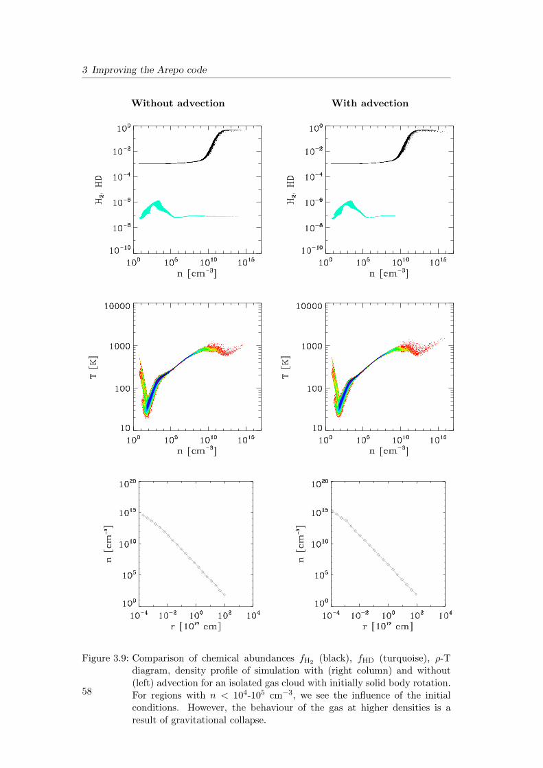
3 Improving the Arepo code
Without advection With advection
Figure 3.9: Comparison of chemical abundances fH2 (black), fHD (turquoise), ρ-Tdiagram, density profile of simulation with (right column) and without(left) advection for an isolated gas cloud with initially solid body rotation.For regions with n < 104-105 cm−3, we see the influence of the initialconditions. However, the behaviour of the gas at higher densities is aresult of gravitational collapse.
58

3.3 Results
Without advection With advection
Figure 3.10: Comparison of chemical abundances fH2 (turquoise), fHD (black), ρ-Tdiagram, with (right column) and without (left) cell-to-cell advection ina cosmological setup.
59
3 Improving the Arepo code
As shown in Fig. 3.10, for a realistic cosmological initial condition, where there ismore turbulent motions and therefore more flux between cell surfaces, introduction ofcell-to-cell advection of chemical species makes a noticeable difference; it results in amore tight correlation between density and fH2 or fHD. There is also less scatter inthe ρ-T diagram.
60

4 Criterion for the formation of HD in theearly universe
4.1 Introduction
In primordial gas, which consists of only light elements produced by cosmic nucle-osynthesis such as hydrogen, deuterium, helium and lithium, the elements responsiblefor most of the cooling in the local ISM (C, O, Si etc.) are absent. In such anenvironment, the hydrogen molecule (H2) is the most important coolant. However,cooling due to H2 is inefficient at low temperatures (T < 200 K) because its lowestenergy rotational transition has an energy of E/kB ∼ 512 K. On the other hand, itsdeuterated analogue, HD is able to cool the gas down below 100 K because its lowestaccessible rotational transition occurs at much lower energy, E/kB ∼ 130 K. In thelow density primordial gas, [HD/H2] is much larger than the cosmic ratio of [D/H]∼ 2.6 × 10⁻⁵, obtained from absorption features in the spectra of distant systems(Burles and Tytler, 1998). This phenomenon is known as fractionation and arises dueto the temperature dependence of the chemical reaction rates, which we will describebelow. The chemical reactions that governs the abundance of HD are (Galli and Palla1998, Galli and Palla 2002):
H2 + D+ → HD + H+ (4.1)
HD + H+ → H2 + D+. (4.2)
The destruction process of HD is slow at low temperatures because of its endothermicnature, so the abundance of HD is boosted at low temperatures. In equilibrium, theHD-to-H2 ratio follows
[HD/H2] = 2 exp
[464
T
][D/H]. (4.3)
If sufficient amount of H2 is present and the gas is cooled enough, then according toequation (4.3), HD abundance is boosted (in other words, reaction (4.1) is favoured),which allows the gas to cool even farther. Since the Jeans mass, the amount of massnecessary for gas clouds to become dynamically unstable (discussed in Section 1.9),changes as a function of density and temperature, how much HD forms in the earlyuniverse, and thus the extent to which primordial gas is able to cool and reduce itsJeans mass has a critical importance for the mass spectrum of the first generationof stars. However, there is also an opposing view about the role that HD plays inprimordial star formation (Clark et al., 2011a), stating that more HD leads to lessfragmentation. The latter adopts two sets of initial conditions to model two different
61

4 HD formation
groups of Pop III stars, and since the initial conditions for the HD-rich case start froma higher abundance of electrons and ionized medium than in truly primordial cases,they are probing a slightly different regime than investigated here; thus care shouldbe taken when comparing the results.
Since the very early works of Abel et al. (2002), Bromm et al. (2002), and Yoshidaet al. (2003) many attempts have been made to numerically model the formation ofprotostars (Bromm, 2013). It is now known that the mass of protostars has somescatter and is different from halo to halo (for example, O’Shea and Norman, 2007).If we consider all the works aimed to follow the formation of Pop III protostars todate, many experiments have been performed to sample the whole spectrum of Pop-ulation III (Pop III) stars. There are also some works that focus on the role that HDmolecules play in the process of primordial star formation (Ripamonti, 2007; McGreerand Bryan, 2008). However, very few cosmological hydrodynamic simulations to dateare dedicated to answer the simple question, ‘what determines the amount of HD thatforms during protostellar collapse?’.
HD is known to form in primordial gas that has a higher than usual abundance ofelectrons, such as in pristine gas clouds that have been exposed to the UV photonsfrom previous generations of star formation. This is because the reaction (4.1) pro-ceeds faster for highly ionized medium, and higher ionisation facilitates H2 formationby reaction (4.4), which results in lower temperature, which leads to an increase inHD abundance (according to equation (4.3)).
H + e− → H− + γ (4.4)
H− + H → H2 + e− (4.5)
In the case of the ‘very first’ Pop III stars to form, or Pop III stars that form inlocations where there are no previous history of star formation, there is no radiationemitted by previous generation of stars. Under such conditions, HD was believedto form only in gas experiencing shocks such as when the dark matter haloes aremerging. This idea was proposed by Shchekinov and Vasiliev (2006) and investigatedby numerical experiment by Bovino et al. (2014), who compare primordial gas collapsetaking place in an isolated halo and in a halo experiencing violent merging events.
However, according to our inspection of the density maps of collapsing gas insideour cosmological simulations, we found no evidence of gas clumps colliding with eachother out of 10 realizations. We conclude that the gas clouds that experience collisionswith neighbouring gas clumps during their collapse (as investigated by Bovino et al.2014) are very rare in number, and are in no way representative of numerous samplesof dark matter haloes. Hirano et al. (2014) hints that the rotation of primordial gasdelays collapse and thus allows for primordial gas to cool sufficiently, and form HD.They resort to comparison with one-zone simulations to make this point.
In this work, we ran many samples of moderate-resolution 3D cosmological hydrody-namical simulations, and without further assumptions, try to discover simple physicalcriteria that accounts for the abundance of HD molecules in primordial mini-haloes.
62

4.2 Numerical methods
4.2 Numerical methods
The initial conditions of our simulations presented here are generated in the followingway: First, we ran collisionless N -body simulations with 1 Mpc/h comoving in lengthwith uniform mass resolution to capture collapsing dark matter haloes starting atz=100. We employ cosmological parameters consistent with the WMAP-7 measure-ments (Ωm = 0.271, ΩΛ = 0.729, σ8 = 0.809, h = 0.703; Komatsu et al., 2011)1 Thesecollisionless simulations were executed with Gadget-3 (Springel et al., 2005). Fromthis parent simulation, we generate a new set of initial conditions (zoom-in ICs) withfiner dark matter resolution at the region of interest, where a specific mini-halo iden-tified by friends-of-friends method that is present at the end of the parent simulationis located. The selected dark matter halo is shifted to the centre of the simulationbox. The regions further away from this specific halo is represented by dark matterparticles with progressively lower resolution. The parent simulation contains 5123
particles, at the regions of interest the mass of the dark matter particles are improvedby 43 (dark matter particle mass of 7.3 M). The results presented in this chapteranalyses simulation outputs initiated from 10 zoom-in ICs, each centred on a differentFOF halo from a single parent simulation. Therefore, they represent different regionsin the same cosmological box.
From this newly generated initial condition with improved dark matter resolution,we start a hydrodynamical simulation with the moving-mesh code AREPO (Springel,2010). During start-up of our hydrodynamic simulations, the code generates gas cellsfrom dark matter only initial conditions. In order to numerically follow the dynamicsof pristine gas in a cosmological context, we adopt on-the-fly mass refinement schemeaccording to Jeans length (32 cells per Jeans length in the production run, 8 cellsper Jeans length for lower resolution comparison run shown in Section 4.4). In orderto study abundance of HD in the early stages of protostellar collapse, we stop oursimulation when the maximum density in the simulation domain reaches ' 106 cm−3.In each timestep, the time-dependent chemical network and associated heating andcooling is solved for each gas cell (see Section 3.1).
4.3 Results
This chapter is intended to clarify the difference between HD-rich and HD-poor gasclouds. In doing so, the actual definition of the amount of HD in a given gas cloud isalso critical. It is better to use mass-weighted HD abundance above certain densitylimit than using the HD abundance of the highest abundance cell. The mass-weightedHD abundance shows good numerical convergence, when the maximum value of HDabundance of individual cells can differ by a factor of few when the refinement criterionis changed. (See also Section 4.4.) In Chapter 3, we have defined fHD as a fractionalabundance of HD with respect to protons. In this chapter, let us define fHD as the
1We would not expect our results to differ significantly if we were to use the cosmological param-eters measured by Planck (Planck Collaboration et al., 2013). This choice of parameters is forconsistency with our previous work Sasaki et al. 2014, see also Chapter 2.
63

4 HD formation
Figure 4.1: Temperatures, abundances of chemical species, and density profiles fordifferent gas clouds. Out of 10 samples of gas clouds, black and brownlines indicate physical properties of gas clouds with the two highest valuesof fHD (mass-weighted average of fractional HD abundance for all cellswith densities > 103 cm−3), and blue and cyan lines indicate those withthe two lowest values of fHD. Note that the gas clouds rich in HD haveless smooth density profiles.
64

4.3 Results
mass-average of previously defined fHD over cells with densities > 103 cm−3, and useit as a measure of HD-richness in each gas cloud.
In Fig. 4.1, we show the temperature, chemical abundances, and the density profileof primordial gas clouds for two most HD-rich clouds (black and brown solid lines)and two most HD-poor clouds (blue and cyan solid lines) out of 10 samples (similarcolor-coding is used for Fig. 4.4). We find that HD-rich clouds have lower temperature(compare densities between 102 and 105 cm−3) than HD-poor clouds. We find thatthe density profiles for HD-rich clouds are noticeably more noisy than the HD-poorclouds. As will be shown in Fig. 4.4, they take longer time to collapse, and haveallowed secondary density perturbations to grow inside the cloud. The comparisonof the density maps illustrated in Fig. 4.2 and 4.3 further clarifies the morphologicaldifferences between HD-rich and HD-poor primordial collapsing gas.
We next study the evolutionary track of the densest point in the primordial gascloud as a function of time (Fig. 4.4) to show that the speed of protostellar collapseis relevant for HD formation. Gas clouds that take longer to collapse tend to havehigher HD fractions. After some numerical experiments, it is discovered that the timeit takes for the central density to evolve from 104 cm−3 to 105 cm−3 is most correlatedwith the amount of HD that is formed. This is probably because HD is mostly formedwhen the density of gas is ≤ 105 cm−3 (see Fig. 4.1). This may apparently seem asa contradiction, as more abundance of HD, or increased HD cooling could hasten thecollapse. However, this is not the case. In the early phase of protostellar formation,the regime we study here, the gas is not supported mainly by thermal energy but bykinetic energy.
As shown in Fig. 4.5, there is a clear relationship between fHD and the time it takesthe gas cloud to collapse for the numerous haloes we have simulated, not just for theselected examples shown in Fig. 4.4.
Let us define the parameter fratio as the ratio between tangential component ofvelocity and the Keplerian velocity at the half-mass radius of gas particles includedinside R200 (see Section 1.4 for definition) of a dark matter halo when the central gasdensity reaches 102 cm−3. fratio defined this way characterises the spin of gas in theearly stage in the gravitational collapse.
Fig. 4.6 (left) shows that the dark matter haloes in which the gas collapsed morerecently are more likely to have higher mass. There seems to be little dependence ofcollapse redshift on fHD (Fig. 4.6, right). Fig. 4.7 (left) shows that the correlationbetween fHD and fratio is only weak. There is some physical reasons for this correla-tion, since the tangential component of velocity is likely to delay the collapse. Theseemingly counter-intuitive positive correlation between subhalo mass and collapsetime (namely, more massive subhaloes take longer time to collapse shown in Fig. 4.7,right) is most likely a reflection of the fact that the gas clouds that collapse slowlyallows their host dark matter halo to grow more massive.
Rotation, however, is not the only physical process that could potentially delay thecollapse of primordial gas inside dark matter mini-haloes. We find stronger positivecorrelation between velocity dispersion and fHD (Fig. 4.8). We interpret this resultsuch that turbulent velocity structures play more important role than rotation indelaying the collapse and allowing enough time for HD to form in collapsing primordial
65

4 HD formation
Figure 4.2: Density slice through the densest point of gas for HD-poor gas clouds atthe final output time when the central density has reached 106 cm−3. Thecircle indicates a radius of 1 proper pc, while the numbers on the axisindicate coordinates in comoving kpc/h. Compare with Fig. 4.3.
66

4.3 Results
Figure 4.3: Density slice through the densest point of gas for HD-rich gas clouds atthe final output time when the central density has reached 106 cm−3. Thecircle indicates a radius of 1 proper pc, while the numbers on the axisindicate coordinates in comoving kpc/h. Compare with Fig. 4.2.
67

4 HD formation
Figure 4.4: Central density of gas clouds as a function of time before collapse (originof time is at the final time in the simulation). The numbers in the legendindicate value of fHD. The clouds that result in high abundance of HD atthe end of simulation (when the central density reaches 106 cm−3) takelonger time to collapse.
Figure 4.5: Relation between collapse time and fHD. ‘Collapse time’ is defined as thetime when the central density increases from 104 to 105 cm−3.
68

4.4 Numerical convergence
Figure 4.6: Relation between the subhalo mass and the collapse redshift (left). Re-lation between the collapse redshift and fHD (right). All physical valuesare at the final output time when the maximum density of gas reaches 106
cm−3. The collapse redshift is the redshift at the final output time.
gas clouds.
4.4 Numerical convergence
In order to confirm that the HD abundance we are measuring is stable even if wechange the refinement criterion, it is important to run the same simulation withdifferent resolution to check for numerical convergence. It is shown that as we increasethe number of cells per Jeans length, the redshift at which the central gas densityreaches 106 cm−3 is made slightly later in time, and the HD abundance of the highestabundance cell in a particular dark matter halo is slightly increased. As shown inFig. 4.9, the temperature, the abundances of chemical species, and the density profileshow good convergence.
4.5 Conclusion
In this chapter, by directly measuring the time it takes for the central density to reacha certain value, just from arguments based on outputs of 3D realistic cosmologicalhydrodynamical simulations, we have clarified that the speed of the gravitationalcollapse determines the amount of HD molecules in primordial gas. We have shownthat disordered velocity fields play a more important role than rotation in delayingthe collapse. In future work, we would like to show this in more detail.
Since this work neglects the effect of radiation from Pop III stars or the heavyelements produced by them, which becomes important after star formation starts to
69

4 HD formation
Figure 4.7: Relation between fHD and fratio (left). Relation between the subhalo massand the collapse time (right). All physical values are at the final outputtime, except for fratio (the ratio between tangential component of velocityand the Keplerian velocity, evaluated at the half-mass radius of gas cellsinside R200), which is measured when the central density reaches 102 cm−3.
Figure 4.8: Correlation between fHD and the velocity dispersion in the earlier stages ofcollapse (when the central density is 102 cm−3), evaluated at the half-massradius of gas cells inside R200.
70

4.5 Conclusion
Figure 4.9: Comparison of temperature, abundances of chemical species, and densityprofile for the same gas cloud with different refinement criterion—8 cellsper Jeans length (red solid line) and 32 cells per Jeans length (black solidline).
71

4 HD formation
take place in a specific region of the universe, it is the lowest order approximationto real cosmic history, and in reality, the gas collapsing at lower redshift would beaffected by the neighbouring gas clouds which have collapsed earlier in time.
72

5 Conclusions
In this thesis, we studied the formation of dark matter haloes and Pop III stars in thehigh-redshift universe. We used high-resolution N -body simulations to investigate theproperties of dark matter mini-haloes found at redshifts z ≥ 15 and to quantify thedifferences between these haloes and their more massive lower-redshift counterparts.Using the moving-mesh code AREPO, which we modified according to our needs (de-scribed in Chapter 3), we studied primordial gas initiating gravitational collapse indark matter mini-haloes. By comparing multiple samples of collapsing gas cloudsfrom cosmological simulations, we sought to find out what determines the amount ofHD molecules that forms in primordial gas. Our scientific findings are summarised intwo parts, corresponding to chapters 2 and 4 respectively.
5.1 Small-scale structure formation
• Dark matter haloes found in our simulations have a distribution of spin pa-rameters that is well fitted by a log-normal function around λ = 0.0262, withdispersion σλ = 0.495. This value for λ is similar to the value ∼ 0.03 obtainedby studying more massive objects at z ∼ 0 (e.g. galaxy clusters). The dimen-sionless spin parameter λ is somewhat sensitive to resolution, and hence ourmeasurement of this quantity is by far the most accurate thus far for the massscales investigated in this work.
• We have shown explicitly from output of our simulations and merger trees con-structed from them that the formation time of dark matter haloes, defined asthe time at which the most massive substructure in a FOF halo reaches half ofits final mass, only weakly depends on halo mass over about four orders of mag-nitude (e.g. mass scales of ∼ 103–107 M). At larger mass scales, structures areknown to form in a hierarchical fashion (formation redshift is a monotonicallydecreasing function of halo mass). But on the mass scales investigated here, thisat least partially breaks down. The weak dependence of the formation time onmass is a result of the slope of the power spectrum of density perturbations atthis scale, where it becomes close to the critical value of −3 for which all massperturbations are expected to collapse simultaneously. The scatter in formationtime is ∼ 10 Myr.
• The shapes of haloes are much less spherical and more highly prolate than haloesfound at z ∼ 0. The most frequent value of the sphericity parameter lies between0.4 and 0.45. This could be due to more frequent mergers at high redshift. Themajority of haloes have triaxiality parameter > 0.9. More massive haloes aremore likely to be slightly less spherical and slightly more filamentary (prolate).
73

5 Conclusion
• We have also investigated the relationship between formation time and haloproperties such as shape, virial ratios, and spin which was not studied previouslyfor the scales examined here. On average, haloes that formed more recently(young haloes) have higher values of the virial ratio, are less spherical, and havehigher values of spin when observed at z = 15. This can be understood becausethe time passed between the formation of these young haloes and the end of thesimulation is less than the relaxation time, trelax ∼ 60 Myr, of these haloes.
• Although not expected from excursion set theory, we find that haloes with highspin are more strongly clustered, where clustering is quantified by the two-point correlation function of the positions of different dark matter haloes. Thiscould mean that haloes born in clustered environments experience stronger tidaltorques during their formation.
Now that the properties of dark matter mini-haloes are studied in detail, we shouldrun a separate set of simulations that include baryonic physics. It would be interestingto study how the dark matter properties studied here are connected to the propertiesof the resulting Pop III stars.
5.2 Criterion for HD formation in primordial gas
• We find that the amount of HD that forms in the gas is closely related to thespeed of the gravitational collapse. If the collapse is slow, it allows time for HDmolecules to form, which lowers minimum gas temperatures by a factor of two.
• There are several physical mechanisms that can potentially delay the gravita-tional collapse of gas in dark matter mini-haloes (e.g. turbulence, rotation etc.).Contrary to previous studies, we find that the amount of HD that form in pri-mordial gas depends little on physical properties such as the dark matter halomass, rotation of gas inside the halo, or merger history of the halo. It seemslikely that turbulence (disordered velocity fields) is playing an important role indelaying the collapse.
The direct next step would be to demonstrate the contribution from turbulence androtation in delaying the collapse in a more explicit way. It would also be quite inter-esting to use the HD-rich and the HD-poor gas clouds we investigated in Chapter 4as initial conditions and investigate the differences in their later stages of collapse.
74

Appendix A
Appendix
A.1 Comparison of structure formation simulation at largeand small scales.
As a validity check for the data analysis method we adopt, and to make a qualitativecomparison between structure formation occurring at different scales, we performeda numerical experiment to follow the evolution of gravitational structures at largerscales with relatively small particle numbers. The basic simulation parameters of thiscomparison simulation and the main simulation are listed in Table A.1, where Lbox isthe size of the simulation box, Npar is the number of dark matter particles included inthe simulation, and zfin is the redshift at which we terminate each of the simulations.Since the size of the simulation box differs by two orders of magnitude in the two runs,the mass scales of the gravitational structures found in each of the two runs differ by∼ 106.
In Fig. A.2, we show the formation time of dark matter haloes found in the ‘Large’run, also identified by the method described in Section 2.2.1. These results are con-sistent with the formation times as derived from the Millennium Simulation (Harkeret al., 2006). Comparing Fig. A.2 with Fig. 2.8, a striking difference in the massdependence of the formation time at the two different regimes is recognised: for darkmatter structures present in the z = 0 simulations, the formation redshift decreasesas a function of halo mass. In Fig. A.3, the virial ratios of these haloes is presented(consistent with earlier findings of Hetznecker and Burkert 2006). Comparing withFig. 2.5, it is clear that dark matter structures identified at z = 0 are substantiallycloser to virial equilibrium compared to those at z = 15. In Fig. A.1, the medianvalues of the sphericity parameter and triaxiality parameter are presented, which areconsistent with results obtained from analysing the Millennium Simulation (Bett et al.,
Table A.1: Simulation parameters
Lbox εRun Npar (h−1 Mpc) zfin (h−1 kpc)
Large 5123 100 0 4.0Small 20483 1 15 0.01
75

Appendix A Appendix
Figure A.1: Median of sphericity s and triaxiality T in different mass bins for darkmatter haloes at z = 0. The sphericity and triaxiality are defined byequations (2.10) and (2.11), respectively.
Figure A.2: Formation time of dark matter haloes as a function of their mass. Median,20 %, and 80 % values in each mass bin are plotted. More massive darkmatter haloes form at smaller redshift.
76
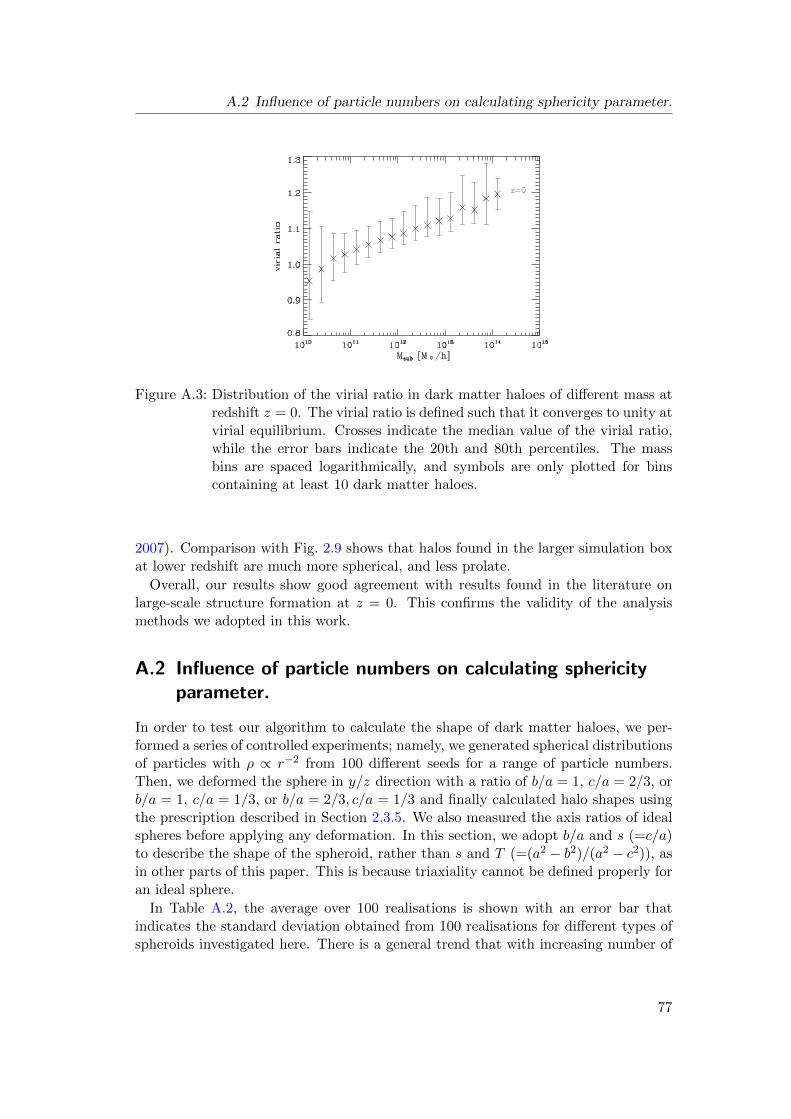
A.2 Influence of particle numbers on calculating sphericity parameter.
Figure A.3: Distribution of the virial ratio in dark matter haloes of different mass atredshift z = 0. The virial ratio is defined such that it converges to unity atvirial equilibrium. Crosses indicate the median value of the virial ratio,while the error bars indicate the 20th and 80th percentiles. The massbins are spaced logarithmically, and symbols are only plotted for binscontaining at least 10 dark matter haloes.
2007). Comparison with Fig. 2.9 shows that halos found in the larger simulation boxat lower redshift are much more spherical, and less prolate.
Overall, our results show good agreement with results found in the literature onlarge-scale structure formation at z = 0. This confirms the validity of the analysismethods we adopted in this work.
A.2 Influence of particle numbers on calculating sphericityparameter.
In order to test our algorithm to calculate the shape of dark matter haloes, we per-formed a series of controlled experiments; namely, we generated spherical distributionsof particles with ρ ∝ r−2 from 100 different seeds for a range of particle numbers.Then, we deformed the sphere in y/z direction with a ratio of b/a = 1, c/a = 2/3, orb/a = 1, c/a = 1/3, or b/a = 2/3, c/a = 1/3 and finally calculated halo shapes usingthe prescription described in Section 2.3.5. We also measured the axis ratios of idealspheres before applying any deformation. In this section, we adopt b/a and s (=c/a)to describe the shape of the spheroid, rather than s and T (=(a2 − b2)/(a2 − c2)), asin other parts of this paper. This is because triaxiality cannot be defined properly foran ideal sphere.
In Table A.2, the average over 100 realisations is shown with an error bar thatindicates the standard deviation obtained from 100 realisations for different types ofspheroids investigated here. There is a general trend that with increasing number of
77

Appendix A Appendix
Table A.2: Convergence study of our method to calculate halo shapes described inSection 2.3.5 using several different types of spheroids. Average and stan-dard deviation is calculated from 100 realisations in each case.
real value No. of particles c/a b/a
100 0.8135 (0.0575) 0.9083 (0.0484)b/a=1, 200 0.8649 (0.0467) 0.9345 (0.0327)c/a=1 500 0.9109 (0.0296) 0.9558 (0.0228)
1000 0.9402 (0.0217) 0.9708 (0.0184)2000 0.9562 (0.0147) 0.9782 (0.0131)
100 0.6209 (0.0557) 0.8917 (0.0528)b/a=1, 200 0.6354 (0.0392) 0.9222 (0.0415)c/a=2/3 500 0.6468 (0.0278) 0.9476 (0.0294)
1000 0.6532 (0.0196) 0.9655 (0.0206)2000 0.6571 (0.0129) 0.9758 (0.0144)
100 0.3099 (0.0293) 0.8822 (0.0600)b/a=1, 200 0.3175 (0.0200) 0.9152 (0.0472)c/a=1/3 500 0.3234 (0.0125) 0.9423 (0.0286)
1000 0.3276 (0.0083) 0.9618 (0.0198)2000 0.3292 (0.0063) 0.9734 (0.0144)
100 0.3286 (0.0325) 0.6647 (0.0635)b/a=2/3, 200 0.3313 (0.0227) 0.6658 (0.0476)c/a=1/3 500 0.3328 (0.0141) 0.6661 (0.0316)
1000 0.3339 (0.0092) 0.6662 (0.0214)2000 0.3334 (0.0064) 0.6658 (0.0138)
78

A.3 Resolution study of the non-dimensional spin parameter
Figure A.4: Non-dimensional spin parameter calculated from high-resolution (20483)simulation and lower-resolution (5123) simulation. Black plus signs de-note ‘main’ subhalo with ≤ 300 particles, green diamonds > 300, ≤ 1000particles, blue triangles > 1000, ≤ 3000 particles, red crosses > 3000particles in the lower resolution simulation.
particles the measured axial ratios become ever closer to the real underlying value,and the standard deviation decreases.
It is shown here that in cases where the underlying values of c/a or b/a are unity,the real value and the estimated value do not match within standard deviations evenwith 2000 particles. Thus, our method tends to underestimate the axial ratios whenthey are close to unity. This tendency was already recognised earlier by Dubinski andCarlberg (1991), who performed similar numerical experiments for their method toestimate halo shapes (their method is not exactly identical to the method we adoptedin this work).
A.3 Resolution study of the non-dimensional spin parameter
Since the non-dimensional spin parameter λ is known to depend severely on how wellthe dark matter structure is resolved, we performed a resolution study by runninga lower-resolution version of our ‘Small’ run with 5123 particles adopting the samecosmological parameters and the same random seed for initial conditions. By matchingdark matter haloes at z = 15 in two different runs according to their positions,we compared the non-dimensional spin parameter. According to Fig. A.4, we findthat haloes with > 1000 particles in the lower resolution run, have relatively goodconvergence. Therefore, for the high-resolution production run, we show the spinparameter of only haloes with ≥ 1000 particles, assuming that they have enoughparticles to capture the intrinsic angular momentum.
79

Appendix A Appendix
A.4 Non-dimensional spin parameter calculated for FOFhaloes
In Fig. A.5, we present the non-dimensional spin parameter calculated for each FOFhaloes as a function of mass. Comparison with Fig. 2.3 shows that FOF gives apositive correlation between spin and halo mass, which is not present for substructuresidentified by SUBFIND.
A.5 Density slice through the whole box.
In Fig. A.6 and A.7, we present the density projection on to the x-y and x-z planesfrom our ‘Small’ and ‘Large’ runs, respectively, in order to illustrate the differencesin structure formation at different scales.
80

A.5 Density slice through the whole box.
Figure A.5: Distribution of the dimensionless spin parameter λ in dark matter haloesof different mass at redshift z ∼ 25 (top panel), z ∼ 20 (middle panel),and z ∼ 15 (bottom panel) calculated for FOF haloes. Crosses indicatethe median value of λ, while the error bars indicate the 20th and 80thpercentiles. The dashed vertical lines represent lower mass limit of 1000particles.
81

Appendix A Appendix
Figure A.6: A density projection on to the x-y (x-z) plane through the centre of thebox with thickness one-fifth of the simulation box size for our ‘Small’ runat z = 15.
Figure A.7: A density projection on to the x-y (x-z) plane through the centre of boxwith thickness one-fifth of the simulation box size for our ‘Large’ run atz = 0.
82

Bibliography
Abel, T., Bryan, G. L., and Norman, M. L. (2002). The Formation of the First Starin the Universe. Science, 295:93–98.
Allgood, B., Flores, R. A., Primack, J. R., Kravtsov, A. V., Wechsler, R. H., Fal-tenbacher, A., and Bullock, J. S. (2006). The shape of dark matter haloes: depen-dence on mass, redshift, radius and formation. MNRAS, 367:1781–1796.
Ballesteros-Paredes, J. (2006). Six myths on the virial theorem for interstellar clouds.MNRAS, 372:443–449.
Barnes, J. and Hut, P. (1986). A hierarchical O(N log N) force-calculation algorithm.Nature, 324:446–449.
Bertschinger, E. and Gelb, J. M. (1991). Cosmological N Body Simulations. Comput-ers in Physics, 5(2).
Bett, P., Eke, V., Frenk, C. S., Jenkins, A., Helly, J., and Navarro, J. (2007). Thespin and shape of dark matter haloes in the Millennium simulation of a Λ cold darkmatter universe. MNRAS, 376:215–232.
Binney, J. and Tremaine, S. (2008). Galactic Dynamics: Second Edition. PrincetonUniversity Press.
Bond, J. R., Cole, S., Efstathiou, G., and Kaiser, N. (1991). Excursion set massfunctions for hierarchical Gaussian fluctuations. ApJ, 379:440–460.
Bond, J. R. and Efstathiou, G. (1984). Cosmic background radiation anisotropies inuniverses dominated by nonbaryonic dark matter. ApJ, 285:L45–L48.
Bouwens, R. J., Illingworth, G. D., Oesch, P. A., Labbe, I., Trenti, M., van Dokkum,P., Franx, M., Stiavelli, M., Carollo, C. M., Magee, D., and Gonzalez, V. (2011).Ultraviolet Luminosity Functions from 132 z ˜ 7 and z ˜ 8 Lyman-break Galaxiesin the Ultra-deep HUDF09 and Wide-area Early Release Science WFC3/IR Obser-vations. ApJ, 737:90.
Bovino, S., Latif, M. A., Grassi, T., and Schleicher, D. R. G. (2014). Dark-matterhalo mergers as a fertile environment for low-mass Population III star formation.MNRAS, 441:2181–2187.
Bromm, V. (2013). Formation of the first stars. Reports on Progress in Physics,76(11):112901.
83

Bibliography
Bromm, V., Coppi, P. S., and Larson, R. B. (2002). The Formation of the First Stars.I. The Primordial Star-forming Cloud. ApJ, 564:23–51.
Bromm, V., Ferrara, A., Coppi, P. S., and Larson, R. B. (2001). The fragmentationof pre-enriched primordial objects. MNRAS, 328:969–976.
Bromm, V. and Loeb, A. (2003). The formation of the first low-mass stars from gaswith low carbon and oxygen abundances. Nature, 425:812–814.
Bromm, V. and Loeb, A. (2004). Accretion onto a primordial protostar. New A,9:353–364.
Bromm, V. and Loeb, A. (2006). High-Redshift Gamma-Ray Bursts from PopulationIII Progenitors. ApJ, 642:382–388.
Bullock, J. S., Kolatt, T. S., Sigad, Y., Somerville, R. S., Kravtsov, A. V., Klypin,A. A., Primack, J. R., and Dekel, A. (2001). Profiles of dark haloes: evolution,scatter and environment. MNRAS, 321:559–575.
Burles, S. and Tytler, D. (1998). The Deuterium Abundance toward Q1937-1009.ApJ, 499:699–712.
Clark, P. C., Glover, S. C. O., and Klessen, R. S. (2008). The First Stellar Cluster.ApJ, 672:757–764.
Clark, P. C., Glover, S. C. O., Klessen, R. S., and Bromm, V. (2011a). Gravita-tional Fragmentation in Turbulent Primordial Gas and the Initial Mass Functionof Population III Stars. ApJ, 727:110.
Clark, P. C., Glover, S. C. O., Smith, R. J., Greif, T. H., Klessen, R. S., and Bromm, V.(2011b). The Formation and Fragmentation of Disks Around Primordial Protostars.Science, 331:1040–.
Crocce, M., Pueblas, S., and Scoccimarro, R. (2006). Transients from initial conditionsin cosmological simulations. MNRAS, 373:369–381.
Dalgarno, A. and McCray, R. A. (1972). Heating and Ionization of HI Regions.ARA&A, 10:375.
Davis, A. J., D’Aloisio, A., and Natarajan, P. (2011). Virialization of high-redshiftdark matter haloes. MNRAS, 416:242–247.
Davis, A. J. and Natarajan, P. (2009). Angular momentum and clustering propertiesof early dark matter haloes. MNRAS, 393:1498–1502.
Davis, A. J. and Natarajan, P. (2010). Spin and structural halo properties at highredshift in a Λ cold dark matter universe. MNRAS, 407:691–703.
Davis, M., Efstathiou, G., Frenk, C. S., and White, S. D. M. (1985). The evolution oflarge-scale structure in a universe dominated by cold dark matter. ApJ, 292:371–394.
84

Bibliography
de Souza, R. S., Ciardi, B., Maio, U., and Ferrara, A. (2013). Dark matter haloenvironment for primordial star formation. MNRAS, 428:2109–2117.
de Souza, R. S., Ishida, E. E. O., Whalen, D. J., Johnson, J. L., and Ferrara, A.(2014). Probing the stellar initial mass function with high-z supernovae. MNRAS,442:1640–1655.
Diemand, J., Kuhlen, M., Madau, P., Zemp, M., Moore, B., Potter, D., and Stadel,J. (2008). Clumps and streams in the local dark matter distribution. Nature,454:735–738.
Dopcke, G., Glover, S. C. O., Clark, P. C., and Klessen, R. S. (2011). The Effect ofDust Cooling on Low-metallicity Star-forming Clouds. ApJ, 729:L3.
Dopcke, G., Glover, S. C. O., Clark, P. C., and Klessen, R. S. (2013). On the InitialMass Function of Low-metallicity Stars: The Importance of Dust Cooling. ApJ,766:103.
Dubinski, J. and Carlberg, R. G. (1991). The structure of cold dark matter halos.ApJ, 378:496–503.
Efstathiou, G., Frenk, C. S., White, S. D. M., and Davis, M. (1988). Gravitationalclustering from scale-free initial conditions. MNRAS, 235:715–748.
Eisenstein, D. J. and Hu, W. (1998). Baryonic Features in the Matter Transfer Func-tion. ApJ, 496:605–614.
Frebel, A. (2010). Stellar archaeology: Exploring the Universe with metal-poor stars.Astronomische Nachrichten, 331:474–488.
Furlanetto, S. R., Oh, S. P., and Briggs, F. H. (2006). Cosmology at low frequencies:The 21 cm transition and the high-redshift Universe. Phys. Rep., 433:181–301.
Galli, D. and Palla, F. (1998). The chemistry of the early Universe. A&A, 335:403–420.
Galli, D. and Palla, F. (2002). Deuterium chemistry in the primordial gas.Planet. Space Sci., 50:1197–1204.
Gao, L., Springel, V., and White, S. D. M. (2005). The age dependence of haloclustering. MNRAS, 363:L66–L70.
Gao, L. and White, S. D. M. (2007). Assembly bias in the clustering of dark matterhaloes. MNRAS, 377:L5–L9.
Gao, L., Yoshida, N., Abel, T., Frenk, C. S., Jenkins, A., and Springel, V. (2007). Thefirst generation of stars in the Λ cold dark matter cosmology. MNRAS, 378:449–468.
Glover, S. (2013). The First Stars. In Wiklind, T., Mobasher, B., and Bromm, V.,editors, Astrophysics and Space Science Library, volume 396 of Astrophysics andSpace Science Library, page 103.
85

Bibliography
Greif, T. H., Bromm, V., Clark, P. C., Glover, S. C. O., Smith, R. J., Klessen,R. S., Yoshida, N., and Springel, V. (2012). Formation and evolution of primordialprotostellar systems. MNRAS, 424:399–415.
Greif, T. H., Springel, V., White, S. D. M., Glover, S. C. O., Clark, P. C., Smith,R. J., Klessen, R. S., and Bromm, V. (2011). Simulations on a Moving Mesh: TheClustered Formation of Population III Protostars. ApJ, 737:75.
Hamilton, A. J. S. (1993). Toward Better Ways to Measure the Galaxy CorrelationFunction. ApJ, 417:19.
Harker, G., Cole, S., Helly, J., Frenk, C., and Jenkins, A. (2006). A marked correlationfunction analysis of halo formation times in the Millennium Simulation. MNRAS,367:1039–1049.
Heavens, A. and Peacock, J. (1988). Tidal torques and local density maxima. MNRAS,232:339–360.
Heger, A. and Woosley, S. E. (2002). The Nucleosynthetic Signature of PopulationIII. ApJ, 567:532–543.
Heger, A. and Woosley, S. E. (2010). Nucleosynthesis and Evolution of MassiveMetal-free Stars. ApJ, 724:341–373.
Hetznecker, H. and Burkert, A. (2006). The evolution of the dark halo spin parametersλ and λ’ in a ΛCDM universe: the role of minor and major mergers. MNRAS,370:1905–1914.
Hinshaw, G., Larson, D., Komatsu, E., Spergel, D. N., Bennett, C. L., Dunkley,J., Nolta, M. R., Halpern, M., Hill, R. S., Odegard, N., Page, L., Smith, K. M.,Weiland, J. L., Gold, B., Jarosik, N., Kogut, A., Limon, M., Meyer, S. S., Tucker,G. S., Wollack, E., and Wright, E. L. (2013). Nine-year Wilkinson MicrowaveAnisotropy Probe (WMAP) Observations: Cosmological Parameter Results. ApJS,208:19.
Hirano, S., Hosokawa, T., Yoshida, N., Umeda, H., Omukai, K., Chiaki, G., andYorke, H. W. (2014). One Hundred First Stars: Protostellar Evolution and theFinal Masses. ApJ, 781:60.
Hoekstra, H., Yee, H. K. C., and Gladders, M. D. (2004). Properties of Galaxy DarkMatter Halos from Weak Lensing. ApJ, 606:67–77.
Ishiyama, T., Fukushige, T., and Makino, J. (2009). Variation of the Subhalo Abun-dance in Dark Matter Halos. ApJ, 696:2115–2125.
Ishiyama, T., Rieder, S., Makino, J., Portegies Zwart, S., Groen, D., Nitadori, K.,de Laat, C., McMillan, S., Hiraki, K., and Harfst, S. (2013). The CosmogridSimulation: Statistical Properties of Small Dark Matter Halos. ApJ, 767:146.
86

Bibliography
Jang-Condell, H. and Hernquist, L. (2001). First Structure Formation: A Simulationof Small-Scale Structure at High Redshift. ApJ, 548:68–78.
Katz, N., Hernquist, L., and Weinberg, D. H. (1999). The Clustering of High-RedshiftGalaxies in the Cold Dark Matter Scenario. ApJ, 523:463–479.
Kauffmann, G., Colberg, J. M., Diaferio, A., and White, S. D. M. (1999). Clusteringof galaxies in a hierarchical universe - I. Methods and results at z=0. MNRAS,303:188–206.
Knebe, A., Pearce, F. R., Lux, H., Ascasibar, Y., Behroozi, P., Casado, J., Moran,C. C., Diemand, J., Dolag, K., Dominguez-Tenreiro, R., Elahi, P., Falck, B., Got-tlober, S., Han, J., Klypin, A., Lukic, Z., Maciejewski, M., McBride, C. K., Mer-chan, M. E., Muldrew, S. I., Neyrinck, M., Onions, J., Planelles, S., Potter, D.,Quilis, V., Rasera, Y., Ricker, P. M., Roy, F., Ruiz, A. N., Sgro, M. A., Springel,V., Stadel, J., Sutter, P. M., Tweed, D., and Zemp, M. (2013). Structure finding incosmological simulations: the state of affairs. MNRAS, 435:1618–1658.
Komatsu, E., Smith, K. M., Dunkley, J., and Bennett, C. L. (2011). Seven-yearWilkinson Microwave Anisotropy Probe (WMAP) Observations: Cosmological In-terpretation. ApJS, 192:18.
Lacey, C. and Cole, S. (1994). Merger Rates in Hierarchical Models of Galaxy For-mation - Part Two - Comparison with N-Body Simulations. MNRAS, 271:676.
Law, D. R., Majewski, S. R., and Johnston, K. V. (2009). Evidence for a TriaxialMilky Way Dark Matter Halo from the Sagittarius Stellar Tidal Stream. ApJ,703:L67–L71.
Maccio, A. V., Dutton, A. A., and van den Bosch, F. C. (2008). Concentration, spinand shape of dark matter haloes as a function of the cosmological model: WMAP1,WMAP3 and WMAP5 results. MNRAS, 391:1940–1954.
Makino, J. (2002). An efficient parallel algorithm for O( N2) direct summation methodand its variations on distributed-memory parallel machines. New A, 7:373–384.
Makino, J., Taiji, M., Ebisuzaki, T., and Sugimoto, D. (1997). GRAPE-4: A Mas-sively Parallel Special-Purpose Computer for Collisional N-Body Simulations. ApJ,480:432–446.
Matzner, C. D. (2003). Supernova hosts for gamma-ray burst jets: dynamical con-straints. MNRAS, 345:575–589.
McGreer, I. D. and Bryan, G. L. (2008). The Impact of HD Cooling on the Formationof the First Stars. ApJ, 685:8–20.
McLure, R. J., Dunlop, J. S., Cirasuolo, M., Koekemoer, A. M., Sabbi, E., Stark, D. P.,Targett, T. A., and Ellis, R. S. (2010). Galaxies at z = 6-9 from the WFC3/IRimaging of the Hubble Ultra Deep Field. MNRAS, 403:960–983.
87

Bibliography
Meiksin, A. and Whalen, D. J. (2013). The radio signatures of the first supernovae.MNRAS, 430:2854–2863.
Moore, B., Kazantzidis, S., Diemand, J., and Stadel, J. (2004). The origin and tidalevolution of cuspy triaxial haloes. MNRAS, 354:522–528.
Neto, A. F., Gao, L., Bett, P., Cole, S., Navarro, J. F., Frenk, C. S., White, S. D. M.,Springel, V., and Jenkins, A. (2007). The statistics of Λ CDM halo concentrations.MNRAS, 381:1450–1462.
Nishi, R. (2002). Star Formation in the Primordial Gas: Overview. Progress ofTheoretical Physics Supplement, 147:1–9.
Nozawa, T., Kozasa, T., Umeda, H., Maeda, K., and Nomoto, K. (2003). Dust in theEarly Universe: Dust Formation in the Ejecta of Population III Supernovae. ApJ,598:785–803.
Oguri, M., Takada, M., Okabe, N., and Smith, G. P. (2010). Direct measurement ofdark matter halo ellipticity from two-dimensional lensing shear maps of 25 massiveclusters. MNRAS, 405:2215–2230.
Omukai, K. (2000). Protostellar Collapse with Various Metallicities. ApJ, 534:809–824.
Omukai, K. and Nishi, R. (1998). Formation of Primordial Protostars. ApJ, 508:141–150.
Omukai, K. and Palla, F. (2001). On the Formation of Massive Primordial Stars.ApJ, 561:L55–L58.
Omukai, K. and Palla, F. (2003). Formation of the First Stars by Accretion. ApJ,589:677–687.
O’Shea, B. W. and Norman, M. L. (2007). Population III Star Formation in a ΛCDMUniverse. I. The Effect of Formation Redshift and Environment on ProtostellarAccretion Rate. ApJ, 654:66–92.
Peebles, P. J. E. (1980). The large-scale structure of the universe.
Planck Collaboration, Ade, P. A. R., Aghanim, N., Armitage-Caplan, C., Arnaud, M.,Ashdown, M., Atrio-Barandela, F., Aumont, J., Baccigalupi, C., Banday, A. J., andet al. (2013). Planck 2013 results. XVI. Cosmological parameters. arXiv:1303.5076.
Planck Collaboration, Ade, P. A. R., Aghanim, N., Armitage-Caplan, C., Arnaud, M.,Ashdown, M., Atrio-Barandela, F., Aumont, J., Baccigalupi, C., Banday, A. J.,and et al. (2014). Planck 2013 results. XXIV. Constraints on primordial non-Gaussianity. A&A, 571:A24.
Plewa, T. and Muller, E. (1999). The consistent multi-fluid advection method. A&A,342:179–191.
88

Bibliography
Press, W. H. and Schechter, P. (1974). Formation of Galaxies and Clusters of Galaxiesby Self-Similar Gravitational Condensation. ApJ, 187:425–438.
Prieto, J., Jimenez, R., and Martı, J. (2012). Dark matter merging induced turbulenceas an efficient engine for gas cooling. MNRAS, 419:3092–3108.
Reed, D. S., Bower, R., Frenk, C. S., Jenkins, A., and Theuns, T. (2007). The halomass function from the dark ages through the present day. MNRAS, 374:2–15.
Ripamonti, E. (2007). The role of HD cooling in primordial star formation. MNRAS,376:709–718.
Santoro, F. and Shull, J. M. (2006). Critical Metallicity and Fine-Structure Emissionof Primordial Gas Enriched by the First Stars. ApJ, 643:26–37.
Sasaki, M., Clark, P. C., Springel, V., Klessen, R. S., and Glover, S. C. O. (2014).Statistical properties of dark matter mini-haloes at z ≥ 15. MNRAS, 442:1942–1955.
Schneider, R., Ferrara, A., Salvaterra, R., Omukai, K., and Bromm, V. (2003). Low-mass relics of early star formation. Nature, 422:869–871.
Shchekinov, Y. A. and Vasiliev, E. O. (2006). Formation of HD molecules in mergingdark matter haloes. MNRAS, 368:454–460.
Sheth, R. K. and Tormen, G. (1999). Large-scale bias and the peak background split.MNRAS, 308:119–126.
Smith, R. J., Glover, S. C. O., Clark, P. C., Greif, T., and Klessen, R. S. (2011). Theeffects of accretion luminosity upon fragmentation in the early universe. MNRAS,414:3633–3644.
Springel, V. (2010). E pur si muove: Galilean-invariant cosmological hydrodynamicalsimulations on a moving mesh. MNRAS, 401:791–851.
Springel, V., Wang, J., Vogelsberger, M., Ludlow, A., Jenkins, A., Helmi, A., Navarro,J. F., Frenk, C. S., and White, S. D. M. (2008). The Aquarius Project: the subhaloesof galactic haloes. MNRAS, 391:1685–1711.
Springel, V., White, S. D. M., Jenkins, A., Frenk, C. S., Yoshida, N., Gao, L., Navarro,J., Thacker, R., Croton, D., Helly, J., Peacock, J. A., Cole, S., Thomas, P., Couch-man, H., Evrard, A., Colberg, J., and Pearce, F. (2005). Simulations of the forma-tion, evolution and clustering of galaxies and quasars. Nature, 435:629–636.
Springel, V., White, S. D. M., Tormen, G., and Kauffmann, G. (2001). Populating acluster of galaxies - I. Results at [formmu2]z=0. MNRAS, 328:726–750.
Stacy, A., Greif, T. H., and Bromm, V. (2010). The first stars: formation of binariesand small multiple systems. MNRAS, 403:45–60.
Stacy, A., Greif, T. H., and Bromm, V. (2012). The first stars: mass growth underprotostellar feedback. MNRAS, 422:290–309.
89

Bibliography
Stadel, J., Potter, D., Moore, B., Diemand, J., Madau, P., Zemp, M., Kuhlen, M., andQuilis, V. (2009). Quantifying the heart of darkness with GHALO - a multibillionparticle simulation of a galactic halo. MNRAS, 398:L21–L25.
Stahler, S. W., Palla, F., and Salpeter, E. E. (1986a). Primordial stellar evolution -The pre-main-sequence phase. ApJ, 308:697–705.
Stahler, S. W., Palla, F., and Salpeter, E. E. (1986b). Primordial stellar evolution -The protostar phase. ApJ, 302:590–605.
Susa, H. (2013). The Mass of the First Stars. ApJ, 773:185.
Tasitsiomi, A., Kravtsov, A. V., Gottlober, S., and Klypin, A. A. (2004). DensityProfiles of ΛCDM Clusters. ApJ, 607:125–139.
Tegmark, M., Silk, J., Rees, M. J., Blanchard, A., Abel, T., and Palla, F. (1997).How Small Were the First Cosmological Objects? ApJ, 474:1.
Todini, P. and Ferrara, A. (2001). Dust formation in primordial Type II supernovae.MNRAS, 325:726–736.
Tominaga, N., Umeda, H., and Nomoto, K. (2007). Supernova Nucleosynthesis inPopulation III 13-50 Msolar Stars and Abundance Patterns of Extremely Metal-poor Stars. ApJ, 660:516–540.
Trenti, M., Smith, B. D., Hallman, E. J., Skillman, S. W., and Shull, J. M. (2010). HowWell do Cosmological Simulations Reproduce Individual Halo Properties? ApJ,711:1198–1207.
Turk, M. J., Abel, T., and O’Shea, B. (2009). The Formation of Population IIIBinaries from Cosmological Initial Conditions. Science, 325:601–.
van den Bosch, F. C., Abel, T., Croft, R. A. C., Hernquist, L., and White, S. D. M.(2002). The Angular Momentum of Gas in Protogalaxies. I. Implications for theFormation of Disk Galaxies. ApJ, 576:21–35.
Warren, M. S., Quinn, P. J., Salmon, J. K., and Zurek, W. H. (1992). Dark halosformed via dissipationless collapse. I - Shapes and alignment of angular momentum.ApJ, 399:405–425.
Wechsler, R. H., Bullock, J. S., Primack, J. R., Kravtsov, A. V., and Dekel, A. (2002).Concentrations of Dark Halos from Their Assembly Histories. ApJ, 568:52–70.
Weinmann, S. M. and Lilly, S. J. (2005). The Number and Observability of PopulationIII Supernovae at High Redshifts. ApJ, 624:526–531.
White, S. D. M. (1984). Angular momentum growth in protogalaxies. ApJ, 286:38–41.
90

Wiggins, B., Whalen, D. J., Migenes, V., and Astrophysics Research Group at LosAlamos National Laboratory (2014). Finding the First Cosmic Explosions: Hyper-novae and Pair-Instability Supernovae. In American Astronomical Society MeetingAbstracts #223, volume 223 of American Astronomical Society Meeting Abstracts,page 102.02.
Yoshida, N., Abel, T., Hernquist, L., and Sugiyama, N. (2003). Simulations of EarlyStructure Formation: Primordial Gas Clouds. ApJ, 592:645–663.
Yoshida, N., Omukai, K., and Hernquist, L. (2008). Protostar Formation in the EarlyUniverse. Science, 321:669–.
Yoshida, N., Omukai, K., Hernquist, L., and Abel, T. (2006). Formation of PrimordialStars in a ΛCDM Universe. ApJ, 652:6–25.
Yoshikawa, K., Yoshida, N., and Umemura, M. (2013). Direct Integration of theCollisionless Boltzmann Equation in Six-dimensional Phase Space: Self-gravitatingSystems. ApJ, 762:116.
91