statistical language models based on neural networks - faculty of
TRANSCRIPT
VYSOKE UCENI TECHNICKE V BRNEBRNO UNIVERSITY OF TECHNOLOGY
FAKULTA INFORMACNICH TECHNOLOGIIUSTAV POCITACOVE GRAFIKY A MULTIMEDII
FACULTY OF INFORMATION TECHNOLOGYDEPARTMENT OF COMPUTER GRAPHICS AND MULTIMEDIA
STATISTICAL LANGUAGE MODELS BASED ON NEURALNETWORKS
DISERTACNI PRACEPHD THESIS
AUTOR PRACE Ing. TOMAS MIKOLOVAUTHOR
BRNO 2012

VYSOKE UCENI TECHNICKE V BRNEBRNO UNIVERSITY OF TECHNOLOGY
FAKULTA INFORMACNICH TECHNOLOGIIUSTAV POCITACOVE GRAFIKY A MULTIMEDII
FACULTY OF INFORMATION TECHNOLOGYDEPARTMENT OF COMPUTER GRAPHICS AND MULTIMEDIA
STATISTICKE JAZYKOVE MODELY ZALOZENENA NEURONOVYCH SITICHSTATISTICAL LANGUAGE MODELS BASED ON NEURAL NETWORKS
DISERTACNI PRACEPHD THESIS
AUTOR PRACE Ing. TOMAS MIKOLOVAUTHOR
VEDOUCI PRACE Doc. Dr. Ing. JAN CERNOCKYSUPERVISOR
BRNO 2012
AbstraktStatisticke jazykove modely jsou dulezitou soucastı mnoha uspesnych aplikacı, mezi nezpatrı naprıklad automaticke rozpoznavanı reci a strojovy preklad (prıkladem je znamaaplikace Google Translate). Tradicnı techniky pro odhad techto modelu jsou zalozenyna tzv. N -gramech. Navzdory znamym nedostatkum techto technik a obrovskemu usilıvyzkumnych skupin naprıc mnoha oblastmi (rozpoznavanı reci, automaticky preklad, neu-roscience, umela inteligence, zpracovanı prirozeneho jazyka, komprese dat, psychologieatd.), N -gramy v podstate zustaly nejuspesnejsı technikou. Cılem teto prace je prezen-tace nekolika architektur jazykovych modelu zalozenych na neuronovych sıtıch. Ackolivjsou tyto modely vypocetne narocnejsı nez N -gramove modely, s technikami vyvinutymi vteto praci je mozne jejich efektivnı pouzitı v realnych aplikacıch. Dosazene snızenı poctuchyb pri rozpoznavanı reci oproti nejlepsım N -gramovym modelum dosahuje 20%. Modelzalozeny na rekurentnı neurovove sıti dosahuje nejlepsıch publikovanych vysledku na velmizname datove sade (Penn Treebank).
AbstractStatistical language models are crucial part of many successful applications, such as au-tomatic speech recognition and statistical machine translation (for example well-knownGoogle Translate). Traditional techniques for estimating these models are based on N -gram counts. Despite known weaknesses of N -grams and huge efforts of research commu-nities across many fields (speech recognition, machine translation, neuroscience, artificialintelligence, natural language processing, data compression, psychology etc.), N -gramsremained basically the state-of-the-art. The goal of this thesis is to present various archi-tectures of language models that are based on artificial neural networks. Although thesemodels are computationally more expensive than N -gram models, with the presentedtechniques it is possible to apply them to state-of-the-art systems efficiently. Achievedreductions of word error rate of speech recognition systems are up to 20%, against state-of-the-art N -gram model. The presented recurrent neural network based model achievesthe best published performance on well-known Penn Treebank setup.
Klıcova slovajazykovy model, neuronova sıt’, rekurentnı, maximalnı entropie, rozpoznavanı reci, komp-rese dat, umela inteligence
Keywordslanguage model, neural network, recurrent, maximum entropy, speech recognition, datacompression, artificial intelligence
CitaceTomas Mikolov: Statistical Language Models Based on Neural Networks, disertacnı prace,Brno, FIT VUT v Brne, 2012
Statistical Language Models Based on Neural Net-works
ProhlasenıProhlasuji, ze jsem tuto disertacnı praci vypracoval samostatne pod vedenım Doc. Dr.Ing. Jana Cernockeho. Uvedl jsem vsechny literarnı publikace, ze kterych jsem cerpal.Nektere experimenty byly provedeny ve spolupraci s dalsımi cleny skupiny Speech@FIT,prıpadne se studenty z Johns Hopkins University - toto je v praci vzdy explicitne uvedeno.
. . . . . . . . . . . . . . . . . . . . . . .Tomas Mikolov
Kveten 2012
AcknowledgementsI would like to thank my supervisor Jan Cernocky for allowing me to explore new ap-proaches to standard problems, for his support and constructive criticism of my work,and for his ability to quickly organize everything related to my studies. I am grateful toLukas Burget for many advices he gave me about speech recognition systems, for longdiscussions about many technical details and for his open-minded approach to research.I would also like to thank all members of Speech@FIT group for cooperation, especiallyStefan Kombrink, Oldrich Plchot, Martin Karafiat, Ondrej Glembek and Jirı Kopecky.It was great experience for me to visit Johns Hopkins University during my studies, and Iam grateful to Frederick Jelinek and Sanjeev Khudanpur for granting me this opportunity.I always enjoyed discussions with Sanjeev, who was my mentor during my stay there. Ialso collaborated with other students at JHU, especially Puyang Xu, Scott Novotney andAnoop Deoras. With Anoop, we were able to push state-of-the-art on several standardtasks to new limits, which was the most exciting for me.As my thesis work is based on work of Yoshua Bengio, it was great for me that I couldhave spent several months in his machine learning lab at University of Montreal. I al-ways enjoyed reading Yoshua’s papers, and it was awesome to discuss with him my ideaspersonally.
© Tomas Mikolov, 2012.Tato prace vznikla jako skolnı dılo na Vysokem ucenı technickem v Brne, Fakulte in-formacnıch technologiı. Prace je chranena autorskym zakonem a jejı uzitı bez udelenıopravnenı autorem je nezakonne, s vyjimkou zakonem definovanych prıpadu.
Contents
1 Introduction 4
1.1 Motivation . . . . . . . . . . . . . . . . . . . . . . . . . . . . . . . . . . . . 4
1.2 Structure of the Thesis . . . . . . . . . . . . . . . . . . . . . . . . . . . . . . 6
1.3 Claims of the Thesis . . . . . . . . . . . . . . . . . . . . . . . . . . . . . . . 7
2 Overview of Statistical Language Modeling 9
2.1 Evaluation . . . . . . . . . . . . . . . . . . . . . . . . . . . . . . . . . . . . . 11
2.1.1 Perplexity . . . . . . . . . . . . . . . . . . . . . . . . . . . . . . . . . 11
2.1.2 Word Error Rate . . . . . . . . . . . . . . . . . . . . . . . . . . . . . 14
2.2 N-gram Models . . . . . . . . . . . . . . . . . . . . . . . . . . . . . . . . . . 16
2.3 Advanced Language Modeling Techniques . . . . . . . . . . . . . . . . . . . 17
2.3.1 Cache Language Models . . . . . . . . . . . . . . . . . . . . . . . . . 18
2.3.2 Class Based Models . . . . . . . . . . . . . . . . . . . . . . . . . . . 19
2.3.3 Structured Language Models . . . . . . . . . . . . . . . . . . . . . . 20
2.3.4 Decision Trees and Random Forest Language Models . . . . . . . . . 22
2.3.5 Maximum Entropy Language Models . . . . . . . . . . . . . . . . . . 22
2.3.6 Neural Network Based Language Models . . . . . . . . . . . . . . . . 23
2.4 Introduction to Data Sets and Experimental Setups . . . . . . . . . . . . . 24
3 Neural Network Language Models 26
3.1 Feedforward Neural Network Based Language Model . . . . . . . . . . . . . 27
3.2 Recurrent Neural Network Based Language Model . . . . . . . . . . . . . . 28
3.3 Learning Algorithm . . . . . . . . . . . . . . . . . . . . . . . . . . . . . . . 30
3.3.1 Backpropagation Through Time . . . . . . . . . . . . . . . . . . . . 33
3.3.2 Practical Advices for the Training . . . . . . . . . . . . . . . . . . . 35
3.4 Extensions of NNLMs . . . . . . . . . . . . . . . . . . . . . . . . . . . . . . 37
1
3.4.1 Vocabulary Truncation . . . . . . . . . . . . . . . . . . . . . . . . . . 37
3.4.2 Factorization of the Output Layer . . . . . . . . . . . . . . . . . . . 37
3.4.3 Approximation of Complex Language Model by Backoff N-gram model 40
3.4.4 Dynamic Evaluation of the Model . . . . . . . . . . . . . . . . . . . 40
3.4.5 Combination of Neural Network Models . . . . . . . . . . . . . . . . 42
4 Evaluation and Combination
of Language Modeling Techniques 44
4.1 Comparison of Different Types of Language Models . . . . . . . . . . . . . . 45
4.2 Penn Treebank Dataset . . . . . . . . . . . . . . . . . . . . . . . . . . . . . 46
4.3 Performance of Individual Models . . . . . . . . . . . . . . . . . . . . . . . . 47
4.3.1 Backoff N-gram Models and Cache Models . . . . . . . . . . . . . . 48
4.3.2 General Purpose Compression Program . . . . . . . . . . . . . . . . 49
4.3.3 Advanced Language Modeling Techniques . . . . . . . . . . . . . . . 50
4.3.4 Neural network based models . . . . . . . . . . . . . . . . . . . . . . 51
4.3.5 Combinations of NNLMs . . . . . . . . . . . . . . . . . . . . . . . . 53
4.4 Comparison of Different Neural Network Architectures . . . . . . . . . . . . 54
4.5 Combination of all models . . . . . . . . . . . . . . . . . . . . . . . . . . . . 58
4.5.1 Adaptive Linear Combination . . . . . . . . . . . . . . . . . . . . . . 60
4.6 Conclusion of the Model Combination Experiments . . . . . . . . . . . . . . 61
5 Wall Street Journal Experiments 62
5.1 WSJ-JHU Setup Description . . . . . . . . . . . . . . . . . . . . . . . . . . 62
5.1.1 Results on the JHU Setup . . . . . . . . . . . . . . . . . . . . . . . . 63
5.1.2 Performance with Increasing Size of the Training Data . . . . . . . . 63
5.1.3 Conclusion of WSJ Experiments (JHU setup) . . . . . . . . . . . . . 65
5.2 Kaldi WSJ Setup . . . . . . . . . . . . . . . . . . . . . . . . . . . . . . . . . 66
5.2.1 Approximation of RNNME using n-gram models . . . . . . . . . . . 68
6 Strategies for Training Large Scale Neural Network Language Models 70
6.1 Model Description . . . . . . . . . . . . . . . . . . . . . . . . . . . . . . . . 71
6.2 Computational Complexity . . . . . . . . . . . . . . . . . . . . . . . . . . . 73
6.2.1 Reduction of Training Epochs . . . . . . . . . . . . . . . . . . . . . . 74
6.2.2 Reduction of Number of Training Tokens . . . . . . . . . . . . . . . 74
2
6.2.3 Reduction of Vocabulary Size . . . . . . . . . . . . . . . . . . . . . . 74
6.2.4 Reduction of Size of the Hidden Layer . . . . . . . . . . . . . . . . . 75
6.2.5 Parallelization . . . . . . . . . . . . . . . . . . . . . . . . . . . . . . 75
6.3 Experimental Setup . . . . . . . . . . . . . . . . . . . . . . . . . . . . . . . 76
6.4 Automatic Data Selection and Sorting . . . . . . . . . . . . . . . . . . . . . 76
6.5 Experiments with large RNN models . . . . . . . . . . . . . . . . . . . . . . 78
6.6 Hash-based Implementation of Class-based Maximum Entropy Model . . . 81
6.6.1 Training of Hash-Based Maximum Entropy Model . . . . . . . . . . 82
6.6.2 Results with Early Implementation of RNNME . . . . . . . . . . . . 85
6.6.3 Further Results with RNNME . . . . . . . . . . . . . . . . . . . . . 86
6.6.4 Language Learning by RNN . . . . . . . . . . . . . . . . . . . . . . . 90
6.7 Conclusion of the NIST RT04 Experiments . . . . . . . . . . . . . . . . . . 92
7 Additional Experiments 94
7.1 Machine Translation . . . . . . . . . . . . . . . . . . . . . . . . . . . . . . . 94
7.2 Data Compression . . . . . . . . . . . . . . . . . . . . . . . . . . . . . . . . 96
7.3 Microsoft Sentence Completion Challenge . . . . . . . . . . . . . . . . . . . 98
7.4 Speech Recognition of Morphologically Rich Languages . . . . . . . . . . . 100
8 Towards Intelligent Models of Natural Languages 102
8.1 Machine Learning . . . . . . . . . . . . . . . . . . . . . . . . . . . . . . . . . 103
8.2 Genetic Programming . . . . . . . . . . . . . . . . . . . . . . . . . . . . . . 105
8.3 Incremental Learning . . . . . . . . . . . . . . . . . . . . . . . . . . . . . . . 106
8.4 Proposal for Future Research . . . . . . . . . . . . . . . . . . . . . . . . . . 107
9 Conclusion and Future Work 109
9.1 Future of Language Modeling . . . . . . . . . . . . . . . . . . . . . . . . . . 111
3
Chapter 1
Introduction
1.1 Motivation
From the first day of existence of the computers, people were dreaming about artificial
intelligence - machines that would produce complex behaviour to reach goals specified
by human users. Possibility of existence of such machines has been controversial, and
many philosophical questions were raised - whether the intelligence is not unique only to
humans, or only to animals etc. Very influential work of Alan Turing did show that any
computable problem can be computed by Universal Turing Machine - thus, assuming that
the human mind can be described by some algorithm, Turing Machine is powerful enough
to represent it.
Computers today are Turing-complete, ie. can represent any computable algorithm.
Thus, the main problem is how to find configuration of the machine so that it would
produce desired behaviour that humans consider intelligent. Assuming that the problem
is too difficult to be solved immediately, we can think of several ways that would lead us
towards intelligent machines - we can start with a simple machine that can recognize basic
shapes and images such as written digits, then scale it towards more complex types of
images such as human faces and so on, finally reaching machine that can recognize objects
in the real world as well as humans can.
Other possible way can be to simulate parts of the human brain on the level of indi-
vidual brain cells, neurons. Computers today are capable of realistically simulating the
real world, as can be seen in modern computer games - thus, it seems logical that with
accurate simulation of neurons and more computational power, it should be possible to
simulate the whole human brain one day.
4
Maybe the most popular vision of future AI as seen in science fiction movies are
robots and computers communicating with humans using natural language. Turing himself
proposed a test of intelligence based on ability of the machine to communicate with humans
using natural language [76]. This choice has several advantages - amount of data that
has to be processed can be very small compared to machine that recognizes images or
sounds. Next, machine that will understand just the basic patterns in the language can
be developed first, and scaled up subsequently. The basic level of understanding can
be at level of a child, or a person that learns a new language - even such low level of
understanding is sufficient to be tested, so that it would be possible to measure progress
in ability of the machine to understand the language.
Assuming that we would want to build such machine that can communicate in natural
language, the question is how to do it. Reasonable way would be to mimic learning
processes of humans. A language is learned by observing the real world, recognizing its
regularities, and mapping acoustic and visual signals to higher level representations in
the brain and back - the acoustic and visual signals are predicted using the higher level
representations. Motivation for learning the language is to improve success of humans in
the real world.
The whole learning problem might be too difficult to be solved at once - there are many
open questions regarding importance of individual factors, such as how much data has to
be processed during training of the machine, how important is it to learn the language
jointly with observing real world situations, how important is the innate knowledge, what
is the best formal representation of the language, etc. It might be too ambitious to attempt
to solve all these problems together, and to expect too much from models or techniques
that even do not allow existence of the solution (an example might be the well-known
limitations of finite state machines to represent efficiently longer term patterns).
Important work that has to be mentioned here is the Information theory of Claude
Shannon. In his famous paper Entropy of printed English [66], Shannon tries to estimate
entropy of the English text using simple experiments involving humans and frequency
based models of the language (n-grams based on history of several preceding characters).
The conclusion was that humans are by far better in prediction of natural text than n-
grams, especially as the length of the context is increased - this so-called ”Shannon game”
can be effectively used to develop more precise test of intelligence than the one defined by
Turing. If we assume that the ability to understand the language is equal (or at least highly
5
correlated) to the ability to predict words in a given context, then we can formally measure
quality of our artificial models of natural languages. This AI test has been proposed for
example in [44] and more discussion is given in [42].
While it is likely that attempts to build artificial language models that can understand
text in the same way as humans do just by reading huge quantities of text data is unreal-
istically hard (as humans would probably fail in such task themselves), language models
estimated from huge amounts of data are very interesting due to their practical usage in
wide variety of commercially successful applications. Among the most widely known ones
are the statistical machine translation (for example popular Google Translate) and the
automatic speech recognition.
The goal of this thesis is to describe new techniques that have been developed to
overcome the simple n-gram models that still remain basically state-of-the-art today. To
prove usefulness of the new approaches, empirical results on several standard data sets
will be extensively described. Finally, approaches and techniques that can possibly lead to
automatic language learning by computers will be discussed, together with a simple plan
how this could be achieved.
1.2 Structure of the Thesis
Chapter 2 introduces the statistical language modeling and mathematically defines the
problem. Simple and advanced language modeling techniques are discussed. Also, the
most important data sets that are further used in the thesis are introduced.
Chapter 3 introduces neural network language models and the recurrent architecture,
as well as the extensions of the basic model. The training algorithm is described in detail.
Chapter 4 provides extensive empirical comparison of results obtained with various
advanced language modeling techniques on the Penn Treebank setup, and results after
combination of these techniques.
The Chapter 5 focuses on the results after application of the RNN language model
to standard speech recognition setup, the Wall Street Journal task. Results and com-
parison are provided on two different setups; one is from the Johns Hopkins University
and allows comparison with competitive techniques such as discriminatively trained LMs
and structured LMs, and the other setup was obtained with an open-source ASR toolkit,
Kaldi.
6
Chapter 6 presents further extensions of the basic recurrent neural network language
model that allow efficient training on large data sets. Experiments are performed on data
sets with up to 400 million training tokens with very large neural networks. Results are
reported on state of the art setup for Broadcast News speech recognition (the NIST RT04
task) with a recognizer and baseline models provided by IBM.
Chapter 7 presents further empirical results on various other tasks, such as machine
translation, data compression and others. The purpose of this chapter is to prove that
the developed techniques are very general and easily applicable to other domains where
n-gram models are currently used.
Chapter 8 discusses computational limitations of models that are commonly used for
the statistical language modeling, and provides some insight into how further progress can
be achieved.
Finally, Chapter 9 summarizes the achieved results and concludes the work.
1.3 Claims of the Thesis
The most important original contributions of this thesis are:
• Development of statistical language model based on simple recurrent neural network
• Extensions of the basic recurrent neural network language model:
– Simple classes based on unigram frequency of words
– Joint training of neural network and maximum entropy model
– Adaptation of neural net language models by sorting the training data
– Adaptation of neural net language models by training the model during pro-
cessing of the test data
• Freely available open source toolkit for training RNN-based language models that
can be used to reproduce the described experiments
• Empirical comparison with other advanced language modeling techniques, with new
state of the art results achieved with RNN based LMs on the following tasks:
– Language modeling of Penn Treebank Corpus
– Wall Street Journal speech recognition
7

– NIST RT04 speech recognition
– Data compression of text, machine translation and other tasks
• Analysis of performance of neural net language models (influence of size of the hidden
layer, increasing amount of the training data)
• Discussion about limitations of traditional approaches to language modeling and
open questions for future research
8
Chapter 2
Overview of Statistical Language
Modeling
Statistical language modeling has received a lot of attention in the past decades. Many
different techniques have been proposed, and nearly each of them can provide improve-
ments over the basic trigram model. However, these techniques are usually studied in
isolation. Comparison is made just to the basic models, and often even these basic models
are poorly tuned. It is thus difficult to judge which technique, or combination of tech-
niques, is currently the state-of-the-art in the statistical language modeling. Moreover,
many of the proposed models provide the same information (for example, longer range
cache-like information), and can be seen just as permutations of existing techniques. This
was already observed by Goodman [24], who proposed that different techniques should be
studied jointly.
Another important observation of Goodman was that relative improvements provided
by some techniques tend to decrease as the amount of training data increases. This has
resulted in much scepticism, and some researchers did claim that it is enough to focus on
obtaining the largest possible amount of training data and build simple n-gram models,
sometimes not even focusing much on the smoothing to be sure that the resulting model
is correctly normalized as reported in [11]. The motivation and justification for these
approaches were results on real tasks.
On the other hand, basic statistical language modeling faces serious challenges when it
is applied to inflective or morphologically rich languages (like Russian, Arabic or Czech),
or when the training data are limited and costly to acquire (as it is for spontaneous speech
9
recognition). Maybe even more importantly, several researchers have already pointed out
that building large look-up tables from huge amounts of training data (which is equal to
standard n-gram modeling) is not going to provide the ultimate answer to the language
modeling problem, as because of curse of dimensionality, we will never have that much
data [5].
The other way around, building language models from huge amounts of data (hundreds
of billion words or more) is also a very challenging task, and has received recently a lot
of attention [26]. The problems that arise include smoothing, as well as compression
techniques, because it is practically impossible to store the full n-gram models estimated
from such amount of data in computer memory. While amount of text that is available
on the Internet is ever-increasing and computers are getting faster and memory bigger, we
cannot hope to build a database of all possible sentences that can ever be said.
In this thesis, recurrent neural network language model (RNN LM) which I have re-
cently proposed in [49, 50] is described, and compared to other successful language mod-
eling techniques. Several standard text corpora are used, which allows to provide detailed
and fair comparison to other advanced language modeling techniques. The aim is at
obtaining the best achievable results by combining all studied models, which leads to a
new state of the art performance on the standard setup involving part of Penn Treebank
Corpus.
Next, it is shown that the RNN based language model can be applied to large scale
well-tuned system, and that it provides significant improvements in speech recognition
accuracy. The baseline system for these experiments from IBM (RT04 Broadcast News
speech recognition) has been recently used in the 2010 Summer Workshop at Johns Hop-
kins University [82]. This system was also used as a baseline for a number of papers
concerning novel type of maximum entropy language model, a so-called model M [30] lan-
guage model, which is also used in the performance comparison as it was previously the
state-of-the-art language model on the given task.
Finally, I try to answer some fundamental questions of language modeling. Namely,
whether the progress in the field is illusory, as is sometimes suggested. And ultimately,
why the new techniques did not reach human performance yet, and what might be the
missing parts and the most promising areas for the future research.
10
2.1 Evaluation
2.1.1 Perplexity
Evaluation of quality of different language models is usually done by using either perplexity
or word error rate. Both metrics have some important properties, as well as drawbacks,
which we will briefly mention here. The perplexity (PPL) of word sequence w is defined
as
PPL = K
√√√√ K∏i=1
1
P (wi|w1...i−1)= 2−
1K
∑Ki=1 log2P (wi|w1...i−1) (2.1)
Perplexity is closely related to the cross entropy between the model and some test data1.
It can be seen as exponential of average per-word entropy of some test data. For example,
if the model encodes each word from the test data on average in 8 bits, the perplexity is
256. There are several practical reasons why to use perplexity and not entropy: first, it is
easier to remember absolute values in the usual range of perplexity between 100-200, than
numbers between corresponding 6.64 and 7.64 bits. Second, it looks better to report that
some new technique yields an improvement of 10% in perplexity, rather than 2% reduction
of entropy, although both results are referring to the same improvement (in this example,
we assume baseline perplexity of 200). Probably the most importantly, perplexity can be
easily evaluated (if we have some held out or test data) and as it is closely related to the
entropy, the model which yields the lowest perplexity is in some sense the closest model
to the true model which generated the data.
There has been great effort in the past to discover models which would be the best for
representing patterns found in both real and artificial sequential data, and interestingly
enough, there has been limited cooperation between researchers working in different fields,
which gave rise to high diversity of various techniques that were developed. Natural
language was viewed by many as a special case of sequence of discrete symbols, and its
structure was supposedly best captured by various limited artificial grammars (such as
context free grammar), with strong linguistic motivation.
The question of validity of the statistical approach for describing natural language has
been raised many times in the past, with maybe the most widely known statement coming
from Noam Chomsky:
1For simplification, it is later denoted simply as entropy.
11
The notion ”probability of a sentence” is an entirely useless one, under any known
interpretation of this term. (Chomsky, 1969)
Still, we can consider entropy and perplexity as very useful measures. The simple
reason is that in the real-world applications (such as speech recognizers), there is a strong
positive correlation between perplexity of involved language model and the system’s per-
formance [24].
More theoretical reasons for using entropy as a measure of performance come from
an artificial intelligence point of view [42]. If we want to build an intelligent agent that
will maximize its reward in time, we have to maximize its ability to predict the outcome
of its own actions. Given the fact that such agent is supposed to work in the real world
and it can experience complex regularities including the natural language, we cannot hope
for a success unless this agent has an ability to find and exploit existing patterns in such
data. It is known that Turing machines (or equivalent) have the ability to represent any
algorithm (in other words, any pattern or regularity). However, algorithms that would
find all possible patterns in some data are not known. Contrary, it was proved that such
algorithms cannot exist in general, due to the halting problem (for some algorithms, the
output is not computationally decidable due to potential infinite recursion).
A very inspiring work on this topic was done by Solomonoff [70], who has shown an
optimal solution to the general prediction problem called Algorithmic probability. Despite
the fact that it is uncomputable, it provides very interesting insight into concepts such
as patterns, regularities, information, noise and randomness. Solomonoff’s solution is to
average over all possible (infinitely many) models of given data, while normalizing by their
description length. Algorithmic probability (ALP) of string x is defined as
PM (x) =∞∑i=0
2−|Si(x)|, (2.2)
where PM (x) denotes probability of string x with respect to machine M and |Si(x)| is
the description length of x (or any sequence that starts with x) given the i-th model of
x. Thus, the shortest descriptions dominate the final value of algorithmic probability of
the string x. More information about ALP, as well as proofs of its interesting properties
(for example invariance to the choice of the machine M, as long as M is universal) can be
found in [70].
12
ALP can be used to obtain prior probabilities of any sequential data, thus it provides
theoretical solution to the statistical language modeling. As mentioned before, ALP is
not computable (because of the halting problem), however it is mentioned here to justify
our later experiments with model combination. Different language modeling techniques
can be seen as individual components in eq. 2.2, where instead of using description length
of individual models for normalization, we use the performance of the model on some
validation data to obtain its weight2. More details about concepts such as ALP and
Minimum description length (MDL) will be given in Chapter 8.
Another work worth of mentioning was done by Mahoney [44], who has shown that the
problem of finding the best models of data is actually equal to the problem of general data
compression. Compression can be seen as two problems: data modeling, and coding. Since
coding is optimally solved by Arithmetic coding, data compression can be seen just as a
data modeling problem. Mahoney together with M. Hutter also organize a competition
with the aim to reach the best possible compression results on a given data set (mostly
containing wikipedia text), known as a Hutter prize competition. As the data compression
of text is almost equal to the language modeling task, I follow the same idea and try
to reach the best achievable results on a single well-known data set, the Penn Treebank
Corpus, where it is possible to compare (and combine) results of techniques developed by
several other researchers.
The important drawback of perplexity is that it obscures achieved improvements. Usu-
ally, improvements of perplexity are measured as percentual decrease over the baseline
value, which is a mistaken but widely accepted practice. In Table 2.1, it is shown that
constant perplexity improvement translates to different entropy reductions. For example,
it will be shown in Chapter 7 that advanced LM techniques provide similar relative reduc-
tions of entropy for word and character based models, while perplexity comparison would
completely fail in such case. Thus, perplexity results will be reported as a good measure
for quick comparison, but improvements will be mainly reported by using entropy.
2It can be argued that since most of the models that are commonly used in language modeling arenot Turing-complete - such as finite state machines - using description length of these models would beinappropriate.
13
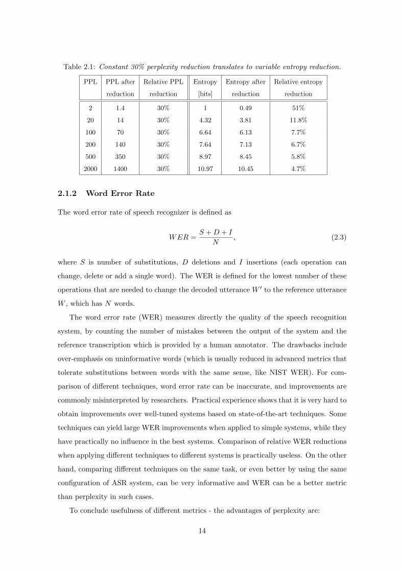
Table 2.1: Constant 30% perplexity reduction translates to variable entropy reduction.
PPL PPL after Relative PPL Entropy Entropy after Relative entropy
reduction reduction [bits] reduction reduction
2 1.4 30% 1 0.49 51%
20 14 30% 4.32 3.81 11.8%
100 70 30% 6.64 6.13 7.7%
200 140 30% 7.64 7.13 6.7%
500 350 30% 8.97 8.45 5.8%
2000 1400 30% 10.97 10.45 4.7%
2.1.2 Word Error Rate
The word error rate of speech recognizer is defined as
WER =S +D + I
N, (2.3)
where S is number of substitutions, D deletions and I insertions (each operation can
change, delete or add a single word). The WER is defined for the lowest number of these
operations that are needed to change the decoded utterance W ′ to the reference utterance
W , which has N words.
The word error rate (WER) measures directly the quality of the speech recognition
system, by counting the number of mistakes between the output of the system and the
reference transcription which is provided by a human annotator. The drawbacks include
over-emphasis on uninformative words (which is usually reduced in advanced metrics that
tolerate substitutions between words with the same sense, like NIST WER). For com-
parison of different techniques, word error rate can be inaccurate, and improvements are
commonly misinterpreted by researchers. Practical experience shows that it is very hard to
obtain improvements over well-tuned systems based on state-of-the-art techniques. Some
techniques can yield large WER improvements when applied to simple systems, while they
have practically no influence in the best systems. Comparison of relative WER reductions
when applying different techniques to different systems is practically useless. On the other
hand, comparing different techniques on the same task, or even better by using the same
configuration of ASR system, can be very informative and WER can be a better metric
than perplexity in such cases.
To conclude usefulness of different metrics - the advantages of perplexity are:
14
• Good theoretical motivation
• Simplicity of evaluation
• Good correlation with system performance
Disadvantages of perplexity are:
• It is hard to check that the reported value is correct (mostly normalization and
”looking into future” related problems)
• Perplexity is often measured assuming perfect history, while this is certainly not true
for ASR systems: poor performance of models that rely on long context information
(such as cache models) is source of confusion and claims that perplexity is not well
correlated with WER
• Most of the research papers compare perplexity values incorrectly - the baseline is
often suboptimal to ”make the results look better”
Advantages of WER:
• Often the final metric we want to optimize; quality of systems is usually measured
by some variation of WER (such as NIST WER)
• Easy to evaluate, as long as we have reference transcriptions
Disadvantages of WER:
• Results are often noisy; for small data sets, the variance in WER results can be
absolutely 0.5%
• Overemphasis on the frequent, uninformative words
• Reference transcriptions can include errors, spelling mistakes
• Substituted words with the same or similar meaning are as bad mistakes as words
that have the opposite meaning
• Full speech recognition system is needed
• Improvements are often task-specific
15
Surprisingly, many research papers come with conclusions such as ”Our model pro-
vides 2% improvement in perplexity over 3-gram with Good-Turing discounting and 0.3%
reduction of WER, thus we have achieved new state of the art results.” - that is clearly mis-
leading statement. Thus, great care must be given to proper evaluation and comparison
of techniques.
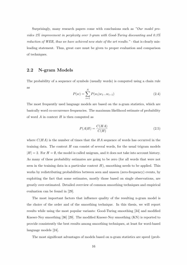
2.2 N-gram Models
The probability of a sequence of symbols (usually words) is computed using a chain rule
as
P (w) =N∑i=1
P (wi|w1...wi−1) (2.4)
The most frequently used language models are based on the n-gram statistics, which are
basically word co-occurrence frequencies. The maximum likelihood estimate of probability
of word A in context H is then computed as
P (A|H) =C(HA)
C(H)(2.5)
where C(HA) is the number of times that the HA sequence of words has occurred in the
training data. The context H can consist of several words, for the usual trigram models
|H| = 2. For H = ∅, the model is called unigram, and it does not take into account history.
As many of these probability estimates are going to be zero (for all words that were not
seen in the training data in a particular context H), smoothing needs to be applied. This
works by redistributing probabilities between seen and unseen (zero-frequency) events, by
exploiting the fact that some estimates, mostly those based on single observations, are
greatly over-estimated. Detailed overview of common smoothing techniques and empirical
evaluation can be found in [29].
The most important factors that influence quality of the resulting n-gram model is
the choice of the order and of the smoothing technique. In this thesis, we will report
results while using the most popular variants: Good-Turing smoothing [34] and modified
Kneser-Ney smoothing [36] [29]. The modified Kneser-Ney smoothing (KN) is reported to
provide consistently the best results among smoothing techniques, at least for word-based
language models [24].
The most significant advantages of models based on n-gram statistics are speed (prob-
16
abilities of n-grams are stored in precomputed tables), reliability coming from simplicity,
and generality (models can be applied to any domain or language effortlessly, as long as
there exists some training data). N-gram models are today still considered as state of the
art not because there are no better techniques, but because those better techniques are
computationally much more complex, and provide just marginal improvements, not critical
for success of given application. Thus, large part of this thesis deals with computational
efficiency and speed-up tricks based on simple reliable algorithms.
The weak part of n-grams is slow adaptation rate when only limited amount of in-
domain data is available. The most important weakness is that the number of possible
n-grams increases exponentially with the length of the context, preventing these models
to effectively capture longer context patterns. This is especially painful if large amounts
of training data are available, as much of the patterns from the training data cannot be
effectively represented by n-grams and cannot be thus discovered during training. The idea
of using neural network based LMs is based on this observation, and tries to overcome the
exponential increase of parameters by sharing parameters among similar events, no longer
requiring exact match of the history H.
2.3 Advanced Language Modeling Techniques
Despite the indisputable success of basic n-gram models, it was always obvious that these
models are not powerful enough to describe language at sufficient level. As an introduc-
tion to the advanced techniques, simple examples will be given first to show what n-grams
cannot do. For example, representation of long-context patters is very inefficient, consider
the following example:
THE SKY ABOVE OUR HEADS IS BLUE
In such sentence, the word BLUE directly depends on the previous word SKY. There is
huge number of possible variations of words between these two that would not break such
relationship - for example, THE SKY THIS MORNING WAS BLUE etc. We can even see that
the number of variations can practically increase exponentially with increasing distance of
the two words from each other in the sentence - we can create many similar sentences for
example by adding all days of week in the sentence, such as:
17
THE SKY THIS <MONDAY, TUESDAY, .., SUNDAY> <MORNING, AFTERNOON, EVENING>
WAS BLUE
N-gram models with N = 4 are unable to efficiently model such common patterns in
the language. With N = 10, we can see that the number of variations is so large that we
cannot realistically hope to have such amounts of training data that would allow n-gram
models to capture such long-context patterns - we would basically have to see each specific
variation in the training data, which is infeasible in practical situations.
Another type of patterns that n-gram models will not be able to model efficiently is
similarity of individual words. A popular example is:
PARTY WILL BE ON <DAY OF WEEK>
Considering that only two or three variations of this sentence are present in the training
data, such as PARTY WILL BE ON MONDAY and PARTY WILL BE ON TUESDAY, the n-gram
models will not be able to assign meaningful probability to novel (but similar) sequence
such as PARTY WILL BE ON FRIDAY, even if days of the week appeared in the training data
frequently enough to discover that there is some similarity among them.
As language modeling is closely related to artificial intelligence and language learning,
it is possible to find great amount of different language modeling techniques and large
number of their variations across research literature published in the past thirty years.
While it is out of scope of this work to describe all of these techniques in detail, we will
at least make short introduction to the important techniques and provide references for
further details.
2.3.1 Cache Language Models
As stated previously, one of the most obvious drawbacks of n-gram models is in their
inability to represent longer term patterns. It has been empirically observed that many
words, especially the rare ones, have significantly higher chance of occurring again if they
did occur in the recent history. Cache models [32] are supposed to deal with this regularity,
and are often represented as another n-gram model, which is estimated dynamically from
the recent history (usually few hundreds of words are considered) and interpolated with the
18
main (static) n-gram model. As the cache models provide truly significant improvements
in perplexity (sometimes even more than 20%), there exists a large number of more refined
techniques that can capture the same patterns as the basic cache models - for example,
various topic models, latent semantic analysis based models [3], trigger models [39] or
dynamically evaluated models [32] [49].
The advantage of cache (or similar) models is in large reduction of perplexity, thus
these techniques are very popular in the language modeling related papers. Also, their
implementation is often quite easy. The problematic part is that new cache-like techniques
are compared to weak baselines, like bigram or trigram models. It is unfair to not include
at least unigram cache model to the baseline, as it is very simple to do so (for example by
using standard LM toolkits such as SRILM [72]).
The main disadvantage is in questionable correlation between perplexity improvements
and word error rate reductions. This has been explained by [24] as a result of the fact
that the errors are locked in the system - if the speech recognizer decodes incorrectly a
word, it is placed in the cache which hurts further recognition by increasing chance of
doing the same error again. When the output from the recognizer is corrected by the user,
cache models are reported to work better; however, it is not practical to force users to
manually correct the output. Advanced versions, like trigger models or LSA models were
reported to provide interesting WER reductions, yet these models are not commonly used
in practice.
Another explanation of poor performance of cache models in speech recognition is
that since the output of a speech recognizer is imperfect, the perplexity calculations that
are normally performed on some held-out data (correct sentences) are misleading. If the
cache models were using the highly ambiguous history of previous words from a speech
recognizer, the perplexity improvements would be dramatically lower. It is thus important
to be careful when conclusions are made about techniques that access very long context
information.
2.3.2 Class Based Models
One way to fight the data sparsity in higher order n-grams is to introduce equivalence
classes. In the simplest case, each word is mapped to a single class, which usually repre-
sents several words. Next, n-gram model is trained on these classes. This allows better
generalization to novel patterns which were not seen in the training data. Improvements
19
are usually achieved by combining class based model and the n-gram model. There exists a
lot of variations of class based models, which often focus on the process of forming classes.
So-called soft classes allow one word to belong to multiple classes. Description of several
variants of class based models can be found in [24].
While perplexity improvements given by class based models are usually moderate, these
techniques have noticeable effect on the word error rate in speech recognition, especially
when only small amount of training data is available. This makes class based models quite
attractive as opposed to the cache models, which usually work well only in experiments
concerning perplexity.
The disadvantages of class based models include high computational complexity during
inference (for statistical classes) or reliance on expert knowledge (for manually assigned
classes). More seriously, improvements tend to vanish with increased amount of the train-
ing data [24]. Thus, class based models are more often found in the research papers, than
in real applications.
From the critical point of view, there are several theoretical difficulties involving class
based models:
• The assumption that words belong to some higher level classes is intuitive, but
usually no special theoretical explanation is given to the process how classes are
constructed; in the end, the number of classes is usually just some tunable parameter
that is chosen based on performance on development data
• Most techniques do attempt to cluster individual words in the vocabulary, but the
idea is not extended to n-grams: by thinking about character-level models, it is obvi-
ous that with increasing amount of the training data, classes can only be successful
if longer context can be captured by a single class (several characters for this case)
2.3.3 Structured Language Models
The statistical language modeling was criticized heavily by the linguists from the first
days of its existence. The already mentioned Chomsky’s statement that ”the notion of
probability of a sentence is completely useless one” can be nowadays easily seen as a big
mistake due to indisputable success of applications that involve n-gram models. However,
further objections from the linguistic community usually address the inability of n-gram
models to represent longer term patterns that clearly exist between words in a sentence.
20
There are many popular examples showing that words in a sentence are often related,
even if they do not lie next to each other. It can be shown that such patterns cannot be
effectively encoded using a finite state machine (n-gram models belong to this family of
computational models). However, these patterns can be often effectively described while
using for example context free grammars.
This was the motivation for the structured language models that attempt to bridge dif-
ferences between the linguistic theories and the statistical models of the natural languages.
The sentence is viewed as a tree structure generated by a context free grammar, where
leafs are individual words and nodes are non-terminal symbols. The statistical approach
is employed when constructing the tree: the derivations have assigned probabilities that
are estimated from the training data, thus every new sentence can be assigned probability
of being generated by the given grammar.
The advantage of these models is in their theoretical ability to represent patterns in
a sentence across many words. Also, these models make language modeling much more
attractive for the linguistic community.
However, there are many practical disadvantages of the structured language models:
• computational complexity and sometimes unstable behaviour (complexity raises non-
linearly with the length of the parsed sentences)
• ambiguity (many different parses are possible)
• questionable performance when applied to spontaneous speech
• large amount of manual work that has to be done by expert linguists is often required,
especially when the technique is to be applied to new domains or new languages,
which can be very costly
• for many languages, it is more difficult to represent sentences using context free
grammars - this is true for example for languages where the concept of word is not
so clear as in English, or where the word order is much more free and not so regular
as it is for English
Despite great research effort in the past decade, the results of these techniques remain
questionable. However, it is certain that the addressed problem - long context patterns
in the natural languages - has to be solved, if we want to get closer towards intelligent
models of languages.
21
2.3.4 Decision Trees and Random Forest Language Models
A decision tree can partition the data in the history by asking question about history at
every node. As these questions can be very general, decision trees were believed to have
a big potential - for example, it is possible to ask questions about presence of specific
word in the history of last ten words. However, in practice it was found that finding good
decision trees can be quite difficult, and even if it can be proved that very good decision
trees exist, usually only suboptimal ones are found by normal training techniques. This
has motivated work on random forest models, which is a combination of many randomly
grown decision trees (linear interpolation is usually used to combine trees into forests).
For more information, see [78].
As the questions in the decision trees can be very general, these models have a possi-
bility to work well for languages with free word order as well as for inflectional languages,
by asking questions about morphology of the words in the history etc. [59]. The drawback
is again high computational complexity. Also, the improvements seem to decrease when
the amount of the training data is large. Thus, these techniques seem to work similar to
the class based models, in some aspects.
2.3.5 Maximum Entropy Language Models
Maximum entropy (ME) model is an exponential model with a form
P (w|h) =e∑
i λifi(w,h)
Z(h)(2.6)
where w is a word in a context h and Z(h) is used for normalizing the probability distri-
bution:
Z(h) =∑wi∈V
e∑
j λjfj(wi,h) (2.7)
thus it can be viewed as a model that combines many feature functions fi(w, h). The
problem of training ME model is to find weights λi of the features, and also to obtain a
good set of these features, as these are not automatically learned from the data. Usual
features are n-grams, skip-grams, etc.
ME models have shown big potential, as they can easily incorporate any features.
Rosenfeld [64] used triggers and word features to obtain very large perplexity improvement,
as well as significant word error rate reduction. There has been a lot of work recently done
22
by Chen et al., who proposed a so-called model M, which is basically a regularized class
based ME model [30]. This model is reported to have a state-of-the-art performance on
a broadcast news speech recognition task [31], when applied to a very well tuned system
that is trained on large amounts of data and uses state of the art discriminatively trained
acoustic models. The significant reductions in WER are reported against a good baseline
language model, 4-gram with modified Kneser-Ney smoothing, across many domains and
tasks. This result is quite rare in the language modeling field, as research papers usually
report improvements over much simpler baseline systems.
An alternative name of maximum entropy models used by the machine learning commu-
nity is logistic regression. While unique algorithms for training ME models were developed
by the speech recognition community (such as Generalized Iterative Scaling), we will show
in Chapter 6 that ME models can be easily trained by stochastic gradient descent. In fact,
it will be later shown that ME models can be seen as a simple neural network without
a hidden layer, and we will exploit this fact to develop novel type of model. Thus, ME
models can be seen as a very general theoretically well founded technique that has already
proven its potential in many fields.
2.3.6 Neural Network Based Language Models
While the clustering algorithms used for constructing class based language models are quite
specific for the language modeling field, artificial neural networks can be successfully used
for dimensionality reduction as well as for clustering, while being a very general machine
learning technique. Thus, it is a bit surprising that neural network based language models
have gained attention only after Y. Bengio’s et al. paper [5] from 2001, and not much
earlier. Although a lot of interesting work on language modeling using neural networks
was done much earlier (for example by Elman [17]), the lack of rigorous comparison to the
state of the art statistical language modeling techniques was missing.
Although it has been very surprising to some, the NNLMs, while very general and
simple, have beaten many of the competing techniques, including those that were devel-
oped specifically for modeling the language. This might not be a coincidence - we may
recall the words of a pioneer of the statistical approaches for automatic speech recognition,
Frederick Jelinek:
23
”Every time I fire a linguist out of my group, the accuracy goes up3.”
We may understand Jelinek’s statement as an observation that with decreased com-
plexity of the system and increased generality of the approaches, the performance goes up.
It is then not so surprising to see the general purpose algorithms to beat the very specific
ones, although clearly the task specific algorithms may have better initial results.
Neural network language models will be described in more detail in Chapter 2. These
models are today among state of the art techniques, and we will demonstrate their per-
formance on several data sets, where on each of them their performance is unmatched by
other techniques.
The main advantage of NNLMs over n-grams is that history is no longer seen as exact
sequence of n − 1 words H, but rather as a projection of H into some lower dimensional
space. This reduces number of parameters in the model that have to be trained, resulting
in automatic clustering of similar histories. While this might sound the same as the
motivation for class based models, the main difference is that NNLMs project all words
into the same low dimensional space, and there can be many degrees of similarity between
words.
The main weak point of these models is very large computational complexity, which
usually prohibits to train these models on full training set, using the full vocabulary. I will
deal with these issues in this work by proposing simple and effective speed-up techniques.
Experiments and results obtained with neural network models trained on over 400M words
while using large vocabulary will be reported, which is to my knowledge the largest set
that a proper NNLM has been trained on4.
2.4 Introduction to Data Sets and Experimental Setups
In this work, I would like to avoid mistakes that are often mentioned when it comes to
criticism of the current research in the statistical language modeling. It is usually claimed
that the new techniques are studied in very specific systems, using weak or ambiguous
baselines. Comparability of the achieved results is very low, if any. This leads to much
3Although later, Jelinek himself claimed that the original statement was ”Every time a linguist leavesmy group, the accuracy goes up”, the former one gained more popularity.
4I am aware of experiments with even more training data (more than 600M words) [8], but the resultingmodel in that work uses a small hidden layer, which as it will be shown later prohibits to train a modelwith competitive performance on such amount of training data.
24
confusion among researchers, and many new results are simply ignored as it is very time
consuming to verify them. To avoid these problems, the performance of the proposed
techniques is studied on very standard tasks, where it is possible to compare achieved
results to baselines that were previously reported by other researchers5.
First, experiments will be shown on a well known Penn Treebank Corpus, and the
comparison will include wide variety of models that were introduced in section 2.3. A
combination of results given by various techniques provides very important information
by showing complementarity of the different language modeling techniques. Final combina-
tion of all techniques that were available to us results in a new state of the art performance
on this particular data set, which is significantly better than of any individual technique.
Second, experiments with increasing amount of the training data will be shown while
using Wall Street Journal training data (NYT Section, the same data as used by [23] [79] [49]).
This study will focus on both entropy and word error rate improvements. The conclusion
seems to be that with increasing amount of the training data, the difference in performance
between the RNN models and the backoff models is getting larger, which is in contrast to
what was found by Goodman [24] for other advanced LM techniques, such as class based
models. Experiments with adaptation of the RNN language models will be shown on this
setup and additional details and results will be provided for another WSJ setup that can
be much more easily replicated, as it is based on a new open-source speech recognition
toolkit, Kaldi [60].
Third, results will be shown for the RNN model applied to the state of the art speech
recognition system developed by IBM [30] that was already briefly mentioned in Sec-
tion 2.3.5, where we will compare the performance to the current state of the art language
model on that set (so-called model M). The language models for this task were trained
on approximately 400M words. Achieved word error rate reductions over the best n-gram
model are relatively over 10%, which is a proof of usefulness of the techniques developed
in this work.
Lastly, comparison of performance of RNN and n-gram models will be provided on a
novel task ”The Microsoft Research Sentence Completion Challenge” [83] that focuses on
ability of artificial language models to appropriately complete a sentence where a single
informative word is missing.
5Many of the experiments described in this work can be reproduced by using a toolkit for trainingRecurrent neural network (RNN) language models which can be found at http://www.fit.vutbr.cz/
~imikolov/rnnlm/.
25
Chapter 3
Neural Network Language Models
The use of artificial neural networks for sequence prediction is as old as the neural network
techniques themselves. One of the first widely known attempts to describe language using
neural networks was performed by Jeff Elman [17], who used recurrent neural network
for modeling sentences of words generated by an artificial grammar. The first serious at-
tempt to build a statistical neural network based language model of real natural language,
together with an empirical comparison of performance to standard techniques (n-gram
models and class based models) was probably done by Yoshua Bengio in [5]. Bengio’s
work was followed by Holger Schwenk, who did show that NNLMs work very well in a
state of the art speech recognition systems, and are complementary to standard n-gram
models [68].
However, despite many scientific papers were published after the original Bengio’s
work, no techniques or modifications of the original model that would significantly improve
ability of the model to capture patterns in the language were published, at least to my
knowledge1. Integration of additional features into the NNLM framework (such as part
of speech tags or morphology information) has been investigated in [19] [1]. Still, the
accuracy of the neural net models remained basically the same, until I have recently shown
that recurrent neural network architecture can work actually better than the feedforward
one [49] [50].
Most of the research work did focus on overcoming practical problems when using
these attractive models: the computational complexity was originally too high for real
world tasks. It was reported by Bengio in 2001 that training of the original neural net
1With the exception of Schwenk, who reported better results by using linear interpolation of severalneural net models trained on the same data, with different random initialization of the weights - we denotethis approach further as a combination of NNLMs.
26
language model took almost a week using 40 CPUs for just a single training epoch (and 10
to 20 epochs were needed for reaching optimal results), despite the fact that only about
14M training words were used (Associated Press News corpus), together with vocabulary
reduced to as little as 18K most frequent words. Moreover, the number of hidden neurons
in the model had to be restricted to just 60, thus the model could not have demonstrated
its full potential. Despite these limitations, the model provided almost 20% reduction of
perplexity over a baseline n-gram model, after 5 training epochs.
Clearly, better results could have been expected if the computational complexity was
not so restrictive, and most of the further research focused on this topic. Bengio proposed
parallel training of the model on several CPUs, which was later repeated and extended by
Schwenk [68]. A very successful extension reduced computation between the hidden layer
and the output layer in the model, using a trick that was originally proposed by Joshua
Goodman for speeding up maximum entropy models [25] - this will be described in more
detail in Section 3.4.2.
3.1 Feedforward Neural Network Based Language Model
The original model proposed by Bengio works as follows: the input of the n-gram NNLM
is formed by using a fixed length history of n− 1 words, where each of the previous n− 1
words is encoded using 1-of-V coding, where V is size of the vocabulary. Thus, every
word from the vocabulary is associated with a vector with length V , where only one value
corresponding to the index of given word in the vocabulary is 1 and all other values are 0.
This 1-of-V orthogonal representation of words is projected linearly to a lower dimen-
sional space, using a shared matrix P , called also a projection matrix. The matrix P is
shared among words at different positions in the history, thus the matrix is the same when
projecting word wt−1, wt−2 etc. In the usual cases, the vocabulary size can be around 50K
words, thus for a 5-gram model the input layer consists of 200K binary variables, while
only 4 of these are set to 1 at any given time, and all others are 0. The projection is done
sometimes into as little as 30 dimensions, thus for our example, the dimensionality of the
projected input layer would be 30 × 4 = 120. After the projection layer, a hidden layer
with non-linear activation function (usually hyperbolic tangent or a logistic sigmoid) is
used, with a dimensionality of 100-300. An output layer follows, with the size equal to the
size of full vocabulary. After the network is trained, the output layer of 5-gram NNLM
27
represents probability distribution P (wt|wt−4, wt−3, wt−2, wt−1).
I have proposed an alternative feedforward architecture of the neural network language
model in [48]. The problem of learning n-gram NNLM is decomposed into two steps:
learning a bigram NNLM (with only the previous word from the history encoded in the
input layer), and then training an n-gram NNLM that projects words from the n-gram
history into the lower dimensional space by using the already trained bigram NNLM. Both
models are simple feedforward neural networks with one hidden layer, thus this solution
is simpler for implementation and for understanding than the original Bengio’s model. It
provides almost identical results as the original model, as will be shown in the following
chapter.
3.2 Recurrent Neural Network Based Language Model
I have described a recurrent neural network language model (RNNLM) in [49] and exten-
sions in [50]. The main difference between the feedforward and the recurrent architecture
is in representation of the history - while for feedforward NNLM, the history is still just
previous several words, for the recurrent model, an effective representation of history is
learned from the data during training. The hidden layer of RNN represents all previous
history and not just n− 1 previous words, thus the model can theoretically represent long
context patterns.
Another important advantage of the recurrent architecture over the feedforward one is
the possibility to represent more advanced patterns in the sequential data. For example,
patterns that rely on words that could have occurred at variable position in the history
can be encoded much more efficiently with the recurrent architecture - the model can
simply remember some specific word in the state of the hidden layer, while the feedforward
architecture would need to use parameters for each specific position of the word in the
history; this not only increases the total amount of parameters in the model, but also the
number of training examples that have to be seen to learn the given pattern.
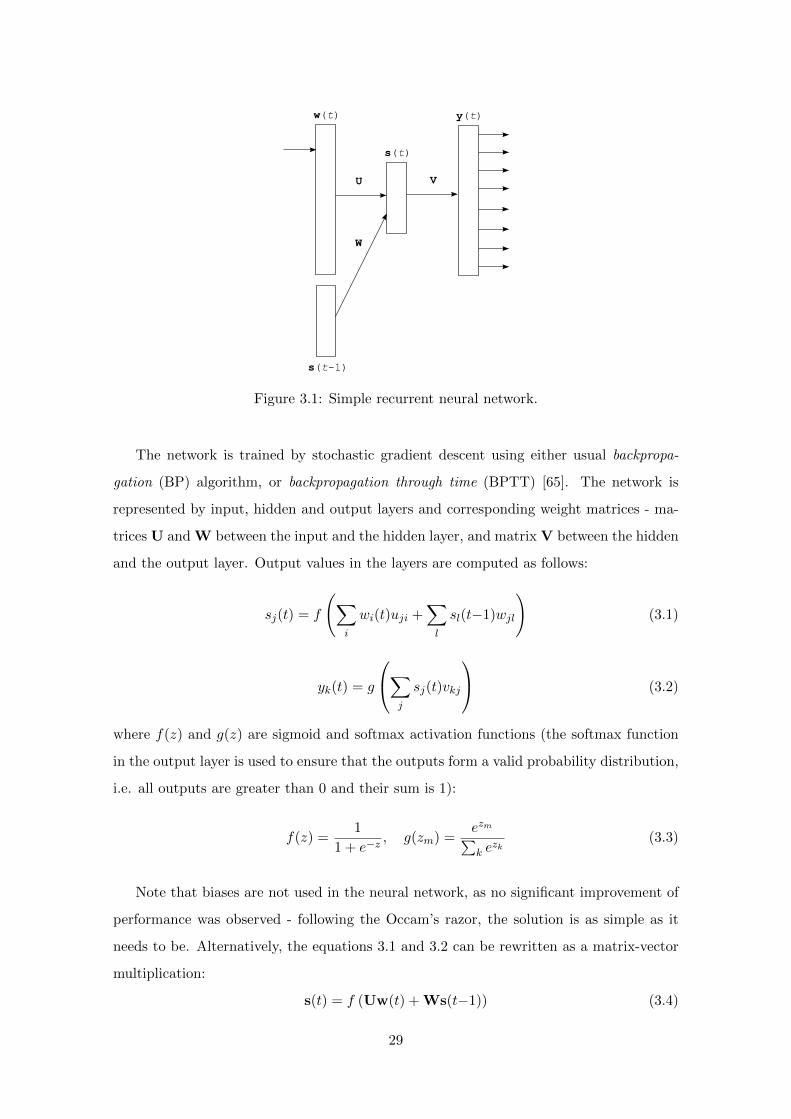
The architecture of RNNLM is shown in Figure 3.1. The input layer consists of a
vector w(t) that represents the current word wt encoded as 1 of V (thus size of w(t) is
equal to the size of the vocabulary), and of vector s(t−1) that represents output values
in the hidden layer from the previous time step. After the network is trained, the output
layer y(t) represents P (wt+1|wt, s(t−1)).
28
U V
y(t)
s(t-1)
s(t)
w(t)
W
Figure 3.1: Simple recurrent neural network.
The network is trained by stochastic gradient descent using either usual backpropa-
gation (BP) algorithm, or backpropagation through time (BPTT) [65]. The network is
represented by input, hidden and output layers and corresponding weight matrices - ma-
trices U and W between the input and the hidden layer, and matrix V between the hidden
and the output layer. Output values in the layers are computed as follows:
sj(t) = f
(∑i
wi(t)uji +∑l
sl(t−1)wjl
)(3.1)
yk(t) = g
∑j
sj(t)vkj
(3.2)
where f(z) and g(z) are sigmoid and softmax activation functions (the softmax function
in the output layer is used to ensure that the outputs form a valid probability distribution,
i.e. all outputs are greater than 0 and their sum is 1):
f(z) =1
1 + e−z, g(zm) =
ezm∑k e
zk(3.3)
Note that biases are not used in the neural network, as no significant improvement of
performance was observed - following the Occam’s razor, the solution is as simple as it
needs to be. Alternatively, the equations 3.1 and 3.2 can be rewritten as a matrix-vector
multiplication:
s(t) = f (Uw(t) + Ws(t−1)) (3.4)
29
y(t) = g (Vs(t)) (3.5)
The output layer y represents a probability distribution of the next word wt+1 given
the history. The time complexity of one training or test step is proportional to
O = H ×H +H × V = H × (H + V ) (3.6)
where H is size of the hidden layer and V is size of the vocabulary.
3.3 Learning Algorithm
Both the feedforward and the recurrent architecture of the neural network model can be
trained by stochastic gradient descent using a well-known backpropagation algorithm [65].
However, for better performance, a so-called Backpropagation through time algorithm can
be used to propagate gradients of errors in the network back in time through the recurrent
weights, so that the model is trained to capture useful information in the state of the
hidden layer. With simple BP training, the recurrent network performs poorly in some
cases, as will be shown later (some comparison was already presented in [50]). The BPTT
algorithm has been described in [65], and a good description for a practical implementation
is in [9].
With the stochastic gradient descent, the weight matrices of the network are updated
after presenting every example. A cross entropy criterion is used to obtain gradient of an
error vector in the output layer, which is then backpropagated to the hidden layer, and in
case of BPTT through the recurrent connections backwards in time. During the training,
validation data are used for early stopping and to control the learning rate. Training
iterates over all training data in several epochs before convergence is achieved - usually,
8-20 epochs are needed. As it will be shown in Chapter 6, the convergence speed of the
training can be improved by randomizing order of sentences in the training data, effectively
reducing the number of required training epochs (this was already observed in [5], and we
provide more details in [52]).
The learning rate is controlled as follows. Starting learning rate is α = 0.1. The
same learning rate is used as long as significant improvement on the validation data is
observed (in further experiments, we consider as a significant improvement more than
0.3% reduction of the entropy). After no significant improvement is observed, the learning
30

rate is halved at start of every new epoch and the training continues until again there is
no improvement. Then the training is finished.
As the validation data set is used only to control the learning rate, it is possible to train
a model even without a validation data, by manually choosing how many epochs should be
performed with the full learning rate, and how many epochs with the decreasing learning
rate. This can be also estimated from experiments with subsets of the training data.
However, in normal cases, it is usual to have a validation data set for reporting perplexity
results. It should be noticed that no over-fitting of the validation data can happen, as the
model does not learn any parameters on such data.
The weight matrices U, V and W are initialized with small random numbers (in
further experiments using normal distribution with mean 0 and variance 0.1) Training of
RNN for one epoch is performed as follows:
1. Set time counter t = 0, initialize state of the neurons in the hidden layer s(t) to 1
2. Increase time counter t by 1
3. Present at the input layer w(t) the current word wt
4. Copy the state of the hidden layer s(t−1) to the input layer
5. Perform forward pass as described in the previous section to obtain s(t) and y(t)
6. Compute gradient of error e(t) in the output layer
7. Propagate error back through the neural network and change weights accordingly
8. If not all training examples were processed, go to step 2
The objective function that we aim to maximize is likelihood of the training data:
f(λ) =
T∑t=1
log ylt(t), (3.7)
where the training samples are labeled t = 1 . . . t, and lt is the index of the correct predicted
word for the t’th sample. Gradient of the error vector in the output layer eo(t) is computed
using a cross entropy criterion that aims to maximize likelihood of the correct class, and
is computed as
eo(t) = d(t)− y(t) (3.8)
31
where d(t) is a target vector that represents the word w(t + 1) that should have been
predicted (encoded again as 1-of-V vector). Note that it is important to use cross entropy
and not mean square error (MSE), which is a common mistake. The network would still
work, but the results would be suboptimal (at least, if our objective is to minimize entropy,
perplexity, word error rate or to maximize compression ratio). Weights V between the
hidden layer s(t) and the output layer y(t) are updated as
vjk(t+1) = vjk(t) + sj(t)eok(t)α (3.9)
where α is the learning rate, j iterates over the size of the hidden layer and k over the
size of the output layer, sj(t) is output of j-th neuron in the hidden layer and eok(t) is
error gradient of k-th neuron in the output layer. If L2 regularization is used, the equation
changes to
vjk(t+1) = vjk(t) + sj(t)eok(t)α− vjk(t)β (3.10)
where β is regularization parameter, in the following experiments its value is β = 10−6.
Regularization is used to keep weights close to zero2. Using matrix-vector notation, the
equation 3.10 would change to
V(t+1) = V(t) + s(t)eo(t)Tα−V(t)β. (3.11)
Next, gradients of errors are propagated from the output layer to the hidden layer
eh(t) = dh(eo(t)
TV, t), (3.12)
where the error vector is obtained using function dh() that is applied element-wise
dhj(x, t) = xsj(t)(1− sj(t)). (3.13)
Weights U between the input layer w(t) and the hidden layer s(t) are then updated as
uij(t+1) = uij(t) + wi(t)ehj(t)α− uij(t)β (3.14)
2Quick explanation of using regularization is by using Occam’s razor: simper solutions should bepreferred, and small numbers can be stored more compactly than the large ones; thus, models with smallweights should generalize better.
32
or using matrix-vector notation as
U(t+1) = U(t) + w(t)eh(t)Tα−U(t)β. (3.15)
Note that only one neuron is active at a given time in the input vector w(t). As can be
seen from the equation 3.14, the weight change for neurons with zero activation is none,
thus the computation can be speeded up by updating weights that correspond just to the
active input neuron. The recurrent weights W are updated as
wlj(t+1) = wlj(t) + sl(t−1)ehj(t)α− wlj(t)β (3.16)
or using matrix-vector notation as
W(t+1) = W(t) + s(t−1)eh(t)Tα−W(t)β (3.17)
3.3.1 Backpropagation Through Time
The training algorithm presented in the previous section is further denoted as normal
backpropagation, as the RNN is trained in the same way as normal feedforward network
with one hidden layer, with the only exception that the state of the input layer depends
on the state of the hidden layer from previous time step.
However, it can be seen that such training approach is not optimal - the network tries
to optimize prediction of the next word given the previous word and previous state of the
hidden layer, but no effort is devoted towards actually storing in the hidden layer state
some information that can be actually useful in the future. If the network remembers
some long context information in the state of the hidden layer, it is so more by luck than
by design.
However, a simple extension of the training algorithm can ensure that the network will
learn what information to store in the hidden layer - this is the so-called Backpropagation
through time algorithm. The idea is simple: a recurrent neural network with one hidden
layer which is used for N time steps can be seen as a deep feedforward network with
N hidden layers (where the hidden layers have the same dimensionality and unfolded
recurrent weight matrices are identical). This idea has already been described in [53], and
is illustrated in Figure 3.2.
Such deep feedforward network can be trained by the normal gradient descent. Errors
33
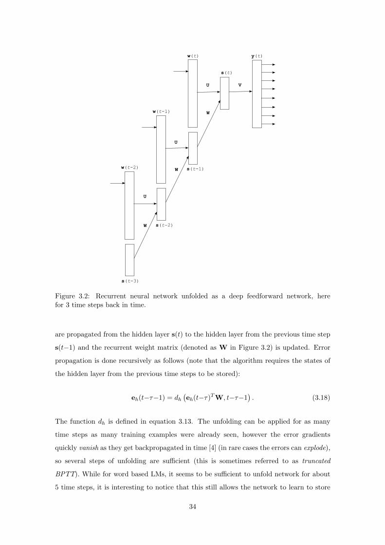
U
s(t-3)
w(t-2)
W
U
U
y(t)
s(t-1)
s(t)
w(t)
s(t-2)
w(t-1)
W
W
V
Figure 3.2: Recurrent neural network unfolded as a deep feedforward network, herefor 3 time steps back in time.
are propagated from the hidden layer s(t) to the hidden layer from the previous time step
s(t−1) and the recurrent weight matrix (denoted as W in Figure 3.2) is updated. Error
propagation is done recursively as follows (note that the algorithm requires the states of
the hidden layer from the previous time steps to be stored):
eh(t−τ−1) = dh(eh(t−τ)TW, t−τ−1
). (3.18)
The function dh is defined in equation 3.13. The unfolding can be applied for as many
time steps as many training examples were already seen, however the error gradients
quickly vanish as they get backpropagated in time [4] (in rare cases the errors can explode),
so several steps of unfolding are sufficient (this is sometimes referred to as truncated
BPTT). While for word based LMs, it seems to be sufficient to unfold network for about
5 time steps, it is interesting to notice that this still allows the network to learn to store
34
information for more than 5 time steps. Similarly, network that is trained by normal
backpropagation can be seen as a network trained with one unfolding step, and still as
we will see later, even this allows the network to learn longer context patterns, such as
4-gram information. The weights U are updated for BPTT training as
uij(t+1) = uij(t) +T∑z=0
wi(t−z)ehj(t−z)α− uij(t)β, (3.19)
where T is the number of steps for which the network is unfolded in time. Alternatively,
equation 3.19 can be written as
U(t+1) = U(t) +T∑z=0
w(t−z)eh(t−z)Tα−U(t)β. (3.20)
It is important to note that the change of the weight matrix U is to be done in one large
update, and not incrementally during the process of backpropagation of errors - that can
lead to instability of the training [9]. Similarly, the recurrent weights W are updated as
wlj(t+1) = wlj(t) +T∑z=0
sl(t−z−1)ehj(t−z)α− wlj(t)β, (3.21)
which is equal to
W(t+1) = W(t) +T∑z=0
s(t−z−1)eh(t−z)Tα−W(t)β. (3.22)
3.3.2 Practical Advices for the Training
While the network can be unfolded for every processed training example, it can be seen
that this would lead to large computational complexity - it would depend on T × W ,
where T is the number of unfolding steps and W is the number of the training words.
However, it can be seen that if the network is unfolded and the recurrent part is trained
only after processing several training examples, the complexity will decrease - in fact, if
the unfolding would be done after processing all the training examples, it can be seen
that the complexity would depend just on W . As in our experiments on-line update of
weights did work better than batch update, it seems to be the best practice to update
recurrent weights in mini-batches (such as after processing 10-20 training examples). This
can effectively remove the term T . The flow of gradients in batch mode training of RNN
35
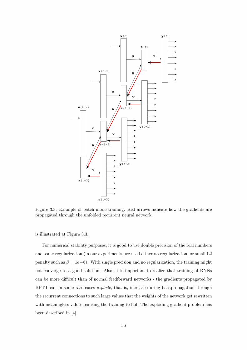
U
W
U
U
V
V
V
w(t-2)
y(t-1)
y(t-2)
y(t-3)
s(t-3)
y(t)
s(t)
w(t)
V
W
Ww(t-1)
s(t-1)
s(t-2)
Figure 3.3: Example of batch mode training. Red arrows indicate how the gradients arepropagated through the unfolded recurrent neural network.
is illustrated at Figure 3.3.
For numerical stability purposes, it is good to use double precision of the real numbers
and some regularization (in our experiments, we used either no regularization, or small L2
penalty such as β = 1e−6). With single precision and no regularization, the training might
not converge to a good solution. Also, it is important to realize that training of RNNs
can be more difficult than of normal feedforward networks - the gradients propagated by
BPTT can in some rare cases explode, that is, increase during backpropagation through
the recurrent connections to such large values that the weights of the network get rewritten
with meaningless values, causing the training to fail. The exploding gradient problem has
been described in [4].
36
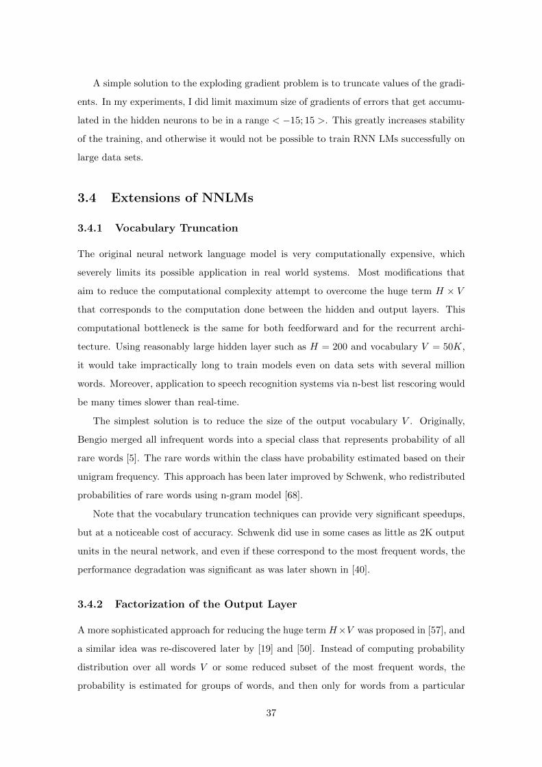
A simple solution to the exploding gradient problem is to truncate values of the gradi-
ents. In my experiments, I did limit maximum size of gradients of errors that get accumu-
lated in the hidden neurons to be in a range < −15; 15 >. This greatly increases stability
of the training, and otherwise it would not be possible to train RNN LMs successfully on
large data sets.
3.4 Extensions of NNLMs
3.4.1 Vocabulary Truncation
The original neural network language model is very computationally expensive, which
severely limits its possible application in real world systems. Most modifications that
aim to reduce the computational complexity attempt to overcome the huge term H × V
that corresponds to the computation done between the hidden and output layers. This
computational bottleneck is the same for both feedforward and for the recurrent archi-
tecture. Using reasonably large hidden layer such as H = 200 and vocabulary V = 50K,
it would take impractically long to train models even on data sets with several million
words. Moreover, application to speech recognition systems via n-best list rescoring would
be many times slower than real-time.
The simplest solution is to reduce the size of the output vocabulary V . Originally,
Bengio merged all infrequent words into a special class that represents probability of all
rare words [5]. The rare words within the class have probability estimated based on their
unigram frequency. This approach has been later improved by Schwenk, who redistributed
probabilities of rare words using n-gram model [68].
Note that the vocabulary truncation techniques can provide very significant speedups,
but at a noticeable cost of accuracy. Schwenk did use in some cases as little as 2K output
units in the neural network, and even if these correspond to the most frequent words, the
performance degradation was significant as was later shown in [40].
3.4.2 Factorization of the Output Layer
A more sophisticated approach for reducing the huge term H×V was proposed in [57], and
a similar idea was re-discovered later by [19] and [50]. Instead of computing probability
distribution over all words V or some reduced subset of the most frequent words, the
probability is estimated for groups of words, and then only for words from a particular
37
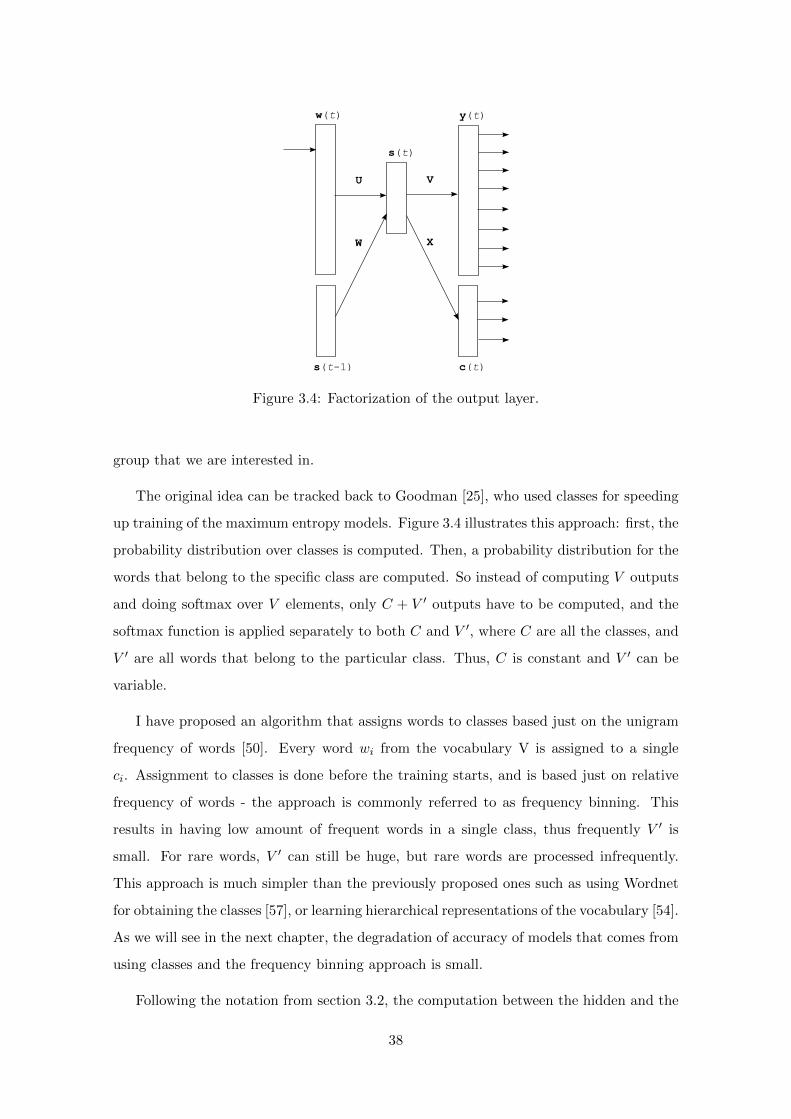
U
y(t)
s(t-1)
s(t)
w(t)
W X
c(t)
V
Figure 3.4: Factorization of the output layer.
group that we are interested in.
The original idea can be tracked back to Goodman [25], who used classes for speeding
up training of the maximum entropy models. Figure 3.4 illustrates this approach: first, the
probability distribution over classes is computed. Then, a probability distribution for the
words that belong to the specific class are computed. So instead of computing V outputs
and doing softmax over V elements, only C + V ′ outputs have to be computed, and the
softmax function is applied separately to both C and V ′, where C are all the classes, and
V ′ are all words that belong to the particular class. Thus, C is constant and V ′ can be
variable.
I have proposed an algorithm that assigns words to classes based just on the unigram
frequency of words [50]. Every word wi from the vocabulary V is assigned to a single
ci. Assignment to classes is done before the training starts, and is based just on relative
frequency of words - the approach is commonly referred to as frequency binning. This
results in having low amount of frequent words in a single class, thus frequently V ′ is
small. For rare words, V ′ can still be huge, but rare words are processed infrequently.
This approach is much simpler than the previously proposed ones such as using Wordnet
for obtaining the classes [57], or learning hierarchical representations of the vocabulary [54].
As we will see in the next chapter, the degradation of accuracy of models that comes from
using classes and the frequency binning approach is small.
Following the notation from section 3.2, the computation between the hidden and the
38
output layer changes to computation between the hidden and the class layer:
cm(t) = g
∑j
sj(t)xmj
, (3.23)
and the hidden layer and a subset of the output layer:
yV ′(t) = g
∑j
sj(t)vV ′j
. (3.24)
The probability of word w(t+ 1) is then computed as
P (wt+1|s(t)) = P (ci|s(t))P (wi|ci, s(t)), (3.25)
where wi is an index of the predicted word and ci is its class. During training, the weights
are accessed in the same way as during the forward pass, thus the gradient of the error
vector is computed for the word part and for the class part, and then is backpropagated
back to the hidden layer, where gradients are added together. Thus, the hidden layer is
trained to predict both the distribution over the words and over the classes.
An alternative to simple frequency binning is a slightly modified approach, that min-
imizes access to words and classes: instead of using frequencies of words for the equal
binning algorithm, one can apply square root function on the original frequencies, and
perform the binning on these modified frequencies. This approach leads to even larger
speed-up3.
Factorization of the computation between the hidden and output layers using simple
classes can easily lead to 15 - 30 times speed-up against a fair baseline, and for the net-
works with huge output layers (more then 100K words), the speedup may be even an order
of magnitude larger. Thus, this speedup trick is essential for achieving reasonable perfor-
mance on larger data sets. Additional techniques for reducing computational complexity
will be discussed in more detail in Chapter 6.
3Thanks to Dan Povey who suggested this modification.
39
3.4.3 Approximation of Complex Language Model by Backoff N-gram
model
In [15], we have shown that NNLM can be partly approximated by a finite state machine.
The conversion is done by sampling words from the probability distribution computed by
NNLM, and a common N-gram model is afterwards trained on the sampled text data.
For infinite amount of sampled data and infinite order N, this approximation technique
is guaranteed to converge to an equivalent model to the one that was used for generating
the words.
Of course, this is not achievable in practice, as it is not possible to generate infinite
amounts of data. However we have shown that even for manageable amounts of sampled
data (hundreds of million words), the approximated model provides some of the improve-
ment over baseline n-gram model that is provided by the full NNLM. Note that this
approach is not limited just to NNLMs or RNNLMs, but can be used to convert any com-
plex model to a finite state representation. However, following the motivation examples
that were shown in the introductory chapter, representing certain patterns using FSMs
is quite impractical, thus we believe this technique can be the most useful for tasks with
limited amount of the training data, where size of models is not so restrictive.
Important advantage of this approach include possibility of using the approximated
model directly during decoding, for the standard lattice rescoring, etc. It is even possible
to use the (R)NNLMs for speech recognition without actually having a single line of neural
net code in the system, as the complex patterns learned by neural net are represented as a
list of possible combinations in the n-gram model. The sampling approach is thus giving
the best possible speedup for the test phase, by trading the computational complexity for
the space complexity.
Empirical results obtained by using this technique for approximating RNNLMs in
speech recognition systems are described in [15] and [38], which is a joint work with
Anoop Deoras and Stefan Kombrink.
3.4.4 Dynamic Evaluation of the Model
From the artificial intelligence point of view, the usual statistical language models have
another drawback besides their inability to represent longer term patterns: the impossibil-
ity to learn new information. This is caused by the fact that LMs are commonly assumed
to be static - the parameters of the models do not change during processing of the data.
40
While RNN models can overcome this disadvantage to some degree by remembering some
information in the hidden layer, due to the vanishing gradient problem it is not possible to
train RNNs to do so using normal gradient based training. Moreover, even if the training
algorithm was powerful enough to discover longer term patterns, it would be inefficient to
store all new information (such as new names of people) in the state of the hidden layer,
and access and update this information at every time step.
The simplest way to overcome this problem is to use dynamic models, which has been
already proposed by Jelinek in [32]. In the case of n-gram models, we can simply train
another n-gram model during processing of the test data based on the recent history, and
interpolate it with the static one - such dynamic model is usually called cache model.
Another approach is to maintain just a single model, and update its parameters online
during processing of the test data. This can be easily achieved using neural network
models.
The disadvantages of using dynamically updated models are that the computational
complexity of the test phase increases, as we need to perform not only the forward pass,
but also calculate gradients and propagate them backwards through the network, and
change weights. More seriously, a network that is presented ambiguous data continually
for significant amount of time steps might forget older information - it can rewrite its own
weights with meaningless information. After the test data switches back to normal data,
the network cannot access the forgotten information anymore. This would not happen
with the n-gram models, since these access parameters very sparsely. Neural net models
share information among all words, thus it is easier to corrupt them.
The dynamic evaluation of the NN language models has been described in my recent
work [49] [50], and is achieved by training the RNN model during processing of the test
data, with a fixed learning rate α = 0.1. Thus, the test data are processed only once,
which is a difference to normal NN training where training data are seen several times.
While the dynamic evaluation of the NN models leads to interesting perplexity im-
provements, especially after combination with the static model (which has the advantage
that it cannot forget any information and cannot be corrupted by the noisy data), ap-
plication to a speech recognition system is very computationally expensive if done in the
exact way, as several versions of the model must be kept in the memory and weights have
to be reloaded to prevent the model to ”see the future” (for example in n-best list rescor-
ing, it is needed to reload weights after processing each hypothesis from a given list). A
41
simplification to the dynamic evaluation is to retrain the NN model on the 1-best utter-
ances, instead of doing a true dynamic evaluation. Both approaches did provide similar
improvements in our experiments.
In [38], we have shown that adaptation of RNN models works better in some cases if
the model is retrained separately on subsets of the test data. In the cited work, it was
shown that for a task of meeting speech recognition, it is a good practice to adapt RNN
LMs on every session in the test data separately.
3.4.5 Combination of Neural Network Models
Since the weights in the neural networks are initialized with small random numbers, every
model converges to a somewhat different solution after the training is finished, even if
the training data are exactly the same. By averaging outputs from several models, it is
possible to obtain better performance - this was already observed by Schwenk [68].
For combining outputs from neural net models, linear interpolation is usually used.
The probability of a word w given N models is then computed as
P (w|h) =N∑i=1
Pi(w|h)
N(3.26)
where Pi(w|h) is a probability estimation of a word w in a context h given by the i-th
model. We can obtain the individual models by simply training several RNN language
models with different random initialization of the weights, or by training RNN models
with different architecture.
Actually, by recalling Algorithmic probability (equation 2.2), we should use infinite
amount of models with all possible architectures, and instead of using equal weights of
models in the combination, an individual model weight should be normalized by the de-
scription length of the model. Computing the description length of any non-trivial model
is intractable4, however we can estimate weights of the models on some validation data.
Practical experience shows that it is the best to train as large models as possible, and to
interpolate models with the same architecture using equal weights.
While I did not perform experiments with combinations of neural net models with
4Sometimes it is assumed that the description length of a model is related to the number of parametersin the model; however, this can be shown to be false, as clearly different parameters require different amountof bits to be stored, and many parameters are often redundant. Moreover, as stated earlier, many patternscan be described using exponentially less parameters by using computationally unrestricted model, thanby using a limited model, such as FSM or a neural net.
42
complex or random architectures (such as more hidden layers, sparse weight matrices etc.),
it can be expected that training models with deep architectures would be very difficult by
using stochastic gradient descent, as vast majority of final solutions are likely to converge
to the same (or similar) local maxima. Thus, the individual solutions are likely to be very
similar in some sense. It might be interesting to explore training techniques that would
produce models with higher diversity, such as evolutionary techniques - although clearly,
that would be a topic for another work.
It is possible to think of using other combination techniques than linear averaging of
probabilities, that can be more useful in the cases when we do not have infinite amount
of possible models of the data. My experiments with log-linear interpolation have shown
only minor improvements over linear interpolation, but since I tried to combine just two
RNN models, more experiments can be done in this direction. Also, it is possible to think
of an additional neural network that would combine the individual models in a non-linear
way: such additional network can be again an RNN model.
We will discuss possible gains that can be obtained by combining outputs from several
RNN models in the next chapter. Also, results when many language modeling techniques
are linearly combined will be presented.
43
Chapter 4
Evaluation and Combination
of Language Modeling Techniques
It is very difficult, if not impossible, to compare different machine learning techniques
just by following their theoretical description. The same holds for the numerous language
modeling techniques: almost every one of them is well-motivated, and some of them even
have theoretical explanation why a given technique is optimal, under certain assumptions.
The problem is that many of such assumptions are not satisfied in practice, when real
data are used.
Comparison of advanced language modeling techniques is usually limited by some of
these factors:
• private data sets that do not allow experiments to be repeated are used
• ad hoc preprocessing is used that favours the proposed technique, or completely
artificial data sets are used
• comparison to proper baseline is completely missing
• baseline technique is not tuned for the best performance
• in comparison, it is falsely claimed that technique X is the state of the art (where X
is usually n-gram model)
• possible comparison to other advanced techniques is done poorly, by citing results
achieved on different data sets, or simply by falsely claiming that the other techniques
are too complex
44
While for any of the previous points I would be able to provide at least several references,
it would be better to define how the new techniques should be evaluated, so that scientific
progress would be measurable:
• experiments should be repeatable: public data sets should be used, or data that are
easily accessible to the scientific community
• techniques that aim to become a new state of the art should be compared not against
the weakest possible baseline, but against the strongest baseline, such as combination
of all known techniques
• to improve repeatability, the code needed for reproducing the experiments should be
released
• review process for accepting papers that propose new techniques should be at least
partially automated, when it comes to verification of the results
While in some cases it might be difficult to satisfy all these points, it is foolish to claim
that new state of the art has been reached, after the perplexity against 3-gram model
drops by 2%; still, such results are still being published at the top level conferences (and
even sometimes win awards as the best papers).
For these reasons, I have decided to release a toolkit that can be used to train RNN
based language models, so that the following experiments can be easily repeated. This
toolkit is introduced and described in Appendix A. Moreover, the following experiments
are performed on well known setups, with direct comparison to competitive techniques.
4.1 Comparison of Different Types of Language Models
It is very difficult to objectively compare different language modeling techniques: in prac-
tical applications, accuracy is sometimes as important as low memory usage and low
computational complexity. Also, the comparison that can be found in the scientific papers
is in some cases unfair, as models that aim to find different type of regularities are some-
times compared. The most obvious example would be a comparison of a long context and
a short context model, such as comparing n-gram model to a cache-like model.
A model that has a potential to discover information only in a few preceding words (like
n-gram model or a class based model) will be further denoted as a ”short-span model”,
while a model that has ability to represent regularities over long range of words (more
45
than a sentence) will be called a ”long-span model”. An example of a long-span model is
a cache model, or a topic model.
Comparison of performance of a short span model (such as 4-gram LM) against a
combination of a short span and a long span model (such as 4-gram + cache) is very
popular in the literature, as it leads to large improvements in perplexity. However, the
reduction of a word error rate in speech recognition by using long-span models is usually
quite small - as was mentioned previously, this is caused by the fact that perplexity is
commonly evaluated while assuming perfect history, which is a false assumption as the
history in speech recognition is typically very noisy1. Typical examples of such experiments
are different novel ways how to compute cache-like models. Joshua Goodman’s report [24]
is a good reference for those who are interested in more insight into criticism of typical
language modeling research.
To avoid these mistakes, performance of individual models is reported and compared
to a modified Kneser-Ney smoothed 5-gram (which is basically a state-of-the-art among
n-gram models), and further compared to a combination of a 5-gram model with a un-
igram cache model. After that, we report the results after using all models together,
with an analysis which models are providing the most complementary information in the
combination, and which models discover patterns that can be better discovered by other
techniques.
4.2 Penn Treebank Dataset
One of the most widely used data sets for evaluating performance of the statistical language
models is the Penn Treebank portion of the WSJ corpus (denoted here as a Penn Treebank
Corpus). It has been previously used by many researchers, with exactly the same data
preprocessing (the same training, validation and test data and the same vocabulary limited
to 10K words). This is quite rare in the language modeling field, and allows us to compare
directly performances of different techniques and their combinations, as many researchers
were kind enough to provide us their results for the following comparison. Combination
of the models is further done by using linear interpolation - for combination of two models
M1 and M2 this means
PM12(w|h) = λPM1(w|h) + (1− λ)PM2(w|h) (4.1)
1Thanks to Dietrich Klakow for pointing this out.
46
where λ is the interpolation weight of the model M1. As long as both models produce
correct probability distributions and λ ∈< 0; 1 >, the linear interpolation produces cor-
rect probability distribution. It has been reported that log-linear interpolation of models
can work in some cases significantly better than the linear interpolation (especially when
combining long span and short span language models), but the log-linear interpolation
requires renormalization of the probability distribution and is thus much more computa-
tionally expensive [35]:
PM12(w|h) =1
Zλ(h)PM1(w|h)λ1 × PM2(w|h)λ2 (4.2)
where Zλ(h) is the normalization term. Because of the normalization term, we need to
consider the full probability distribution given by both models, while for the linear inter-
polation, it is enough to interpolate probabilities given by both models for an individual
word. The previous equations can be easily extended to combination of more than two
models, by having separate weight for each model.
The Penn Treebank Corpus was divided as follows: sections 0-20 were used as the
training data (930k tokens), sections 21-22 as the validation data (74k tokens) and sections
23-24 as the test data (82k tokens). All words outside the 10K vocabulary were mapped to
a special token (unknown word) in all PTB data sets, thus there are no Out-Of-Vocabulary
(OOV) words.
4.3 Performance of Individual Models
The performance of all individual models used in the further experiments is presented in
Table 4.1. First, we will give references and provide brief details about the individual
models. Then we will compare performance of models, combine them together and finally
analyze contributions of all individual models and techniques. I would also like to mention
here that the following experiments were performed with the help of Anoop Deoras who
reimplemented some of the advanced LM techniques that are mentioned in the comparison.
Some of the following results are also based on the work of other researchers, as will be
mentioned later.
47
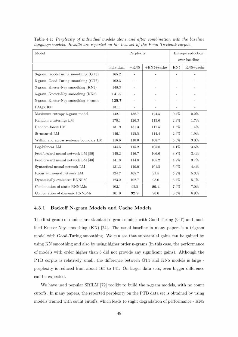
Table 4.1: Perplexity of individual models alone and after combination with the baselinelanguage models. Results are reported on the test set of the Penn Treebank corpus.
Model Perplexity Entropy reduction
over baseline
individual +KN5 +KN5+cache KN5 KN5+cache
3-gram, Good-Turing smoothing (GT3) 165.2 - - - -
5-gram, Good-Turing smoothing (GT5) 162.3 - - - -
3-gram, Kneser-Ney smoothing (KN3) 148.3 - - - -
5-gram, Kneser-Ney smoothing (KN5) 141.2 - - - -
5-gram, Kneser-Ney smoothing + cache 125.7 - - - -
PAQ8o10t 131.1 - - - -
Maximum entropy 5-gram model 142.1 138.7 124.5 0.4% 0.2%
Random clusterings LM 170.1 126.3 115.6 2.3% 1.7%
Random forest LM 131.9 131.3 117.5 1.5% 1.4%
Structured LM 146.1 125.5 114.4 2.4% 1.9%
Within and across sentence boundary LM 116.6 110.0 108.7 5.0% 3.0%
Log-bilinear LM 144.5 115.2 105.8 4.1% 3.6%
Feedforward neural network LM [50] 140.2 116.7 106.6 3.8% 3.4%
Feedforward neural network LM [40] 141.8 114.8 105.2 4.2% 3.7%
Syntactical neural network LM 131.3 110.0 101.5 5.0% 4.4%
Recurrent neural network LM 124.7 105.7 97.5 5.8% 5.3%
Dynamically evaluated RNNLM 123.2 102.7 98.0 6.4% 5.1%
Combination of static RNNLMs 102.1 95.5 89.4 7.9% 7.0%
Combination of dynamic RNNLMs 101.0 92.9 90.0 8.5% 6.9%
4.3.1 Backoff N-gram Models and Cache Models
The first group of models are standard n-gram models with Good-Turing (GT) and mod-
ified Kneser-Ney smoothing (KN) [24]. The usual baseline in many papers is a trigram
model with Good-Turing smoothing. We can see that substantial gains can be gained by
using KN smoothing and also by using higher order n-grams (in this case, the performance
of models with order higher than 5 did not provide any significant gains). Although the
PTB corpus is relatively small, the difference between GT3 and KN5 models is large -
perplexity is reduced from about 165 to 141. On larger data sets, even bigger difference
can be expected.
We have used popular SRILM [72] toolkit to build the n-gram models, with no count
cutoffs. In many papers, the reported perplexity on the PTB data set is obtained by using
models trained with count cutoffs, which leads to slight degradation of performance - KN5
48
model with default SRILM cutoffs provides PPL 148 on the test set, while without cutoffs,
the perplexity is 141. We also report the perplexity of the best n-gram model (KN5) when
using unigram cache model (as implemented in the SRILM toolkit). We have used several
unigram cache models interpolated together, with different lengths of the cache history
(this works like a crude approximation of cache decay, ie. words further in the history
have lower weight). This provides us with the second baseline2.
We are aware of the fact that unigram cache model is not state of the art among cache
models - as reported by Goodman [24], n-gram cache models can provide in some cases
up to twice the improvement that the simple unigram cache model provides. However
due to the fact that we will use later more complex techniques for capturing long context
information in the model combination, we do not consider this to be a significant weakness
in our comparison.
4.3.2 General Purpose Compression Program
PAQ8o10t is a state of the art general purpose compression program3 developed by Ma-
honey et al. [46]. To compute perplexity of the test set using a compression program, we
have first compressed the training set, and then the training set concatenated with the
test set. As there are no new words occurring in the test set of the PTB corpus (all words
outside the 10K vocabulary are rewritten as <unk>), the information that needs to be cap-
tured by a compression program is the same as when using a statistical language model
(this is however not true in cases when the test data contains out of vocabulary words, as
the language modeling techniques usually skip such words for likelihood evaluation). By
subtracting the sizes of the two files, we can measure the amount of bits that were needed
to compress the test data, after the compression program has seen the training data. We
can compute the word-level perplexity, as we know the number of symbols in the test data,
denoted as COUNT (the number of words and end of line symbols), and the number of
bits B that were needed to encode them:
PPL = 2B
COUNT (4.3)
2In fact, performance of many techniques were reported in the past on this data set without actuallyshowing the perplexity when a cache model is used. Such papers include topic models and other techniquesthat aim to capture longer context information, which can be easily captured (to some degree) by a simplecache model. Thus, we consider it important to show results also for the second baseline that includescache, although it makes the comparison in Table 4.1 more difficult to read.
3The benchmark can be found at http://cs.fit.edu/~mmahoney/compression/
49
The resulting perplexity 131.1 given by PAQ is quite good, comparable to the state of the
art backoff model combined with the cache model. This model is however not used in the
model combination, as it would be difficult to obtain probabilities of individual words in
the test set. Also, we do not expect this model to be complementary to the KN5+cache
model.
The PAQ archivers are based on a neural network without a hidden layer, thus the
model is very similar to what is denoted in the language modeling field as a maximum
entropy model. The main difference is that the prediction is based not only on the history
of preceding words, but also on the history of several previous characters. In fact, there
are several other predictors in the model, each using different context (some of them
are specific to other types of data than text). The other interesting difference is that
the prediction of the future data is done on a bit level, which leads to speed up as one
does not have to normalize over all possible characters, or words. Also, the hash-based
implementation of the neural network has been a motivation for our model that will be
introduced in Chapter 6.
4.3.3 Advanced Language Modeling Techniques
The second group of models in Table 4.1 represents popular advanced LM techniques.
Maximum entropy models [64] allow easy integration of any information source in the
probabilistic model. In our study, we have used a model with up to 5-gram features. The
results were obtained by using SRILM extension for training ME models, with the default
L1 and L2 regularization parameters described in [2]. The observed improvement over
baseline KN5 model is rather modest, it can be seen that the ME model with just n-gram
features works about the same as the n-gram model with the best smoothing. It can be
expected that better results can be obtained by having more features in the model, like
triggers or class features.
Random clustering LM is a class based model described in [20]. This model has been
reimplemented for our experiments by Anoop Deoras. We used just simple classes for this
model, but the performance after interpolation with the baseline n-gram model is about
the same as reported by Emami.
We used 4-gram features for the Random forest language model [78], that is a combi-
nation of several randomly grown decision trees. We are aware of several implementations
of structured language models that were previously evaluated on the PTB dataset - in our
50
experiments, we have used the one implemented by Filimonov [23], as it has very competi-
tive performance among structured LMs (PPL 125.5). Better results were reported on this
dataset with another structured LM - in [77], perplexity 118.4 is reported for SuperARV
language model combined with n-gram model; however, we did not have this model for
our experiments.
Within and across sentence boundary LM was proposed in [56]. This model incorpo-
rates several information sources: across sentence boundary model similar to cache, skip
n-gram model and a class based model. Across sentence boundary model works in a very
similar way as a cache model, and the combination with the skip n-gram model and a class
based model is thus quite similar to the combination of models reported by Goodman [24].
The perplexity is reduced considerably over the baseline KN5 model; although it is claimed
in [56] that the performance of the standalone model is state of the art, we have found that
a combination of this model with a KN5 model provides further improvement, resulting
in PPL 110. Adding also our cache model did not improve the results significantly, only
to PPL 108.7. This model performs the best among the non-neural network models, but
one has to keep in mind that the model itself is a combination of several models.
4.3.4 Neural network based models
The third group of models in Table 4.1 consists of individual neural network language
models with different architectures. There are two types of feedforward neural network
models. The first type was proposed in my earlier work and learns the features and
the final model independently while using two neural networks, both with one hidden
layer [48] (see section 3.1). The second and more common type was originally proposed
by Yoshua Bengio [5] - the neural network learns a linear projection of words into a low
dimensional space together with the final model. Both feedforward architectures were
found to have almost identical performance on the PTB setup. The latter model used in
these experiments was implemented by Hai Son Le [40], as well as the log-bilinear model,
which was proposed as an alternative to the neural network language models in [54].
Syntactical neural network language model developed by Emami has been reported
to provide the state of the art results on the Penn Treebank Corpus in [19], and we are
not aware of any better results published since then until our work. It is the only neural
network architecture in our study that actually uses more features in the input layer than
just words - the syntactical information comes from a syntactical parser, thus this model is
51
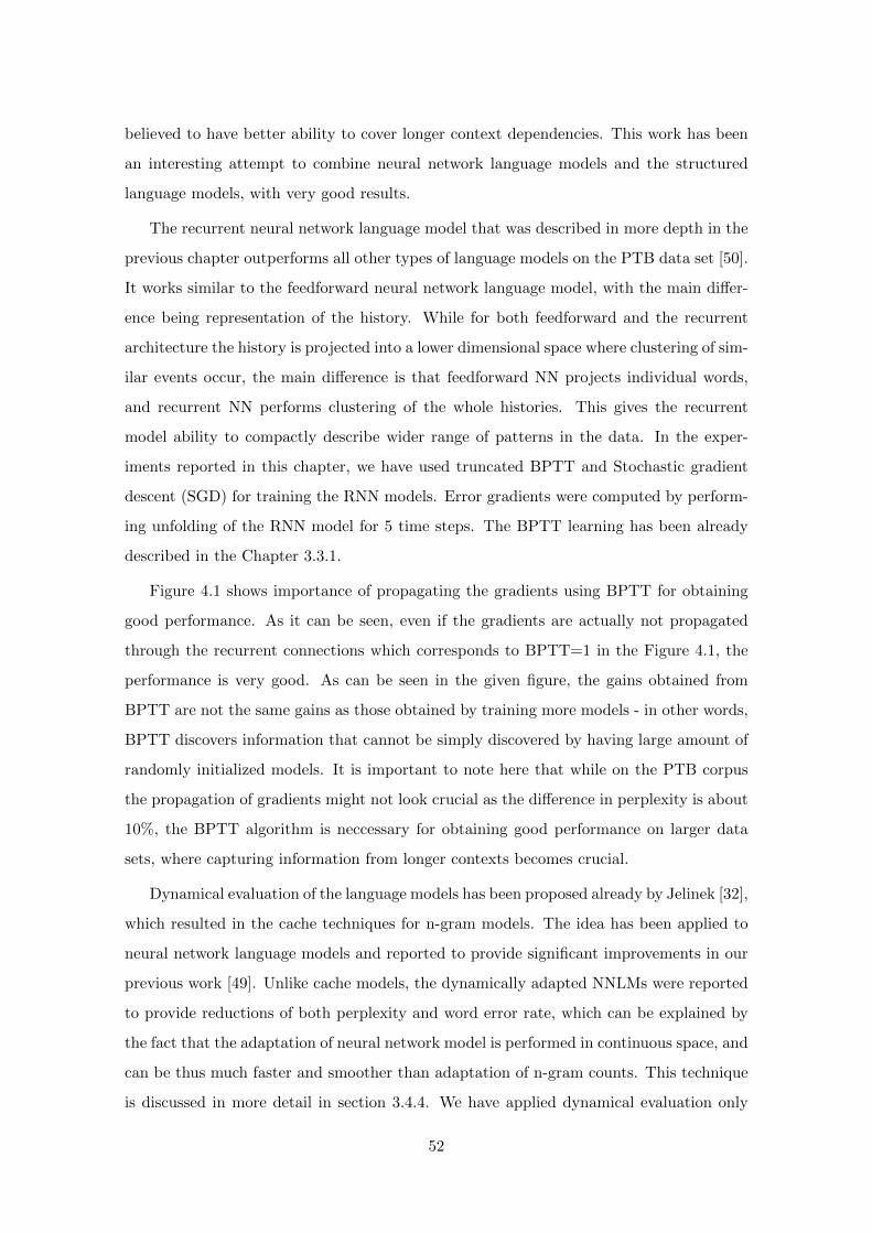
believed to have better ability to cover longer context dependencies. This work has been
an interesting attempt to combine neural network language models and the structured
language models, with very good results.
The recurrent neural network language model that was described in more depth in the
previous chapter outperforms all other types of language models on the PTB data set [50].
It works similar to the feedforward neural network language model, with the main differ-
ence being representation of the history. While for both feedforward and the recurrent
architecture the history is projected into a lower dimensional space where clustering of sim-
ilar events occur, the main difference is that feedforward NN projects individual words,
and recurrent NN performs clustering of the whole histories. This gives the recurrent
model ability to compactly describe wider range of patterns in the data. In the exper-
iments reported in this chapter, we have used truncated BPTT and Stochastic gradient
descent (SGD) for training the RNN models. Error gradients were computed by perform-
ing unfolding of the RNN model for 5 time steps. The BPTT learning has been already
described in the Chapter 3.3.1.
Figure 4.1 shows importance of propagating the gradients using BPTT for obtaining
good performance. As it can be seen, even if the gradients are actually not propagated
through the recurrent connections which corresponds to BPTT=1 in the Figure 4.1, the
performance is very good. As can be seen in the given figure, the gains obtained from
BPTT are not the same gains as those obtained by training more models - in other words,
BPTT discovers information that cannot be simply discovered by having large amount of
randomly initialized models. It is important to note here that while on the PTB corpus
the propagation of gradients might not look crucial as the difference in perplexity is about
10%, the BPTT algorithm is neccessary for obtaining good performance on larger data
sets, where capturing information from longer contexts becomes crucial.
Dynamical evaluation of the language models has been proposed already by Jelinek [32],
which resulted in the cache techniques for n-gram models. The idea has been applied to
neural network language models and reported to provide significant improvements in our
previous work [49]. Unlike cache models, the dynamically adapted NNLMs were reported
to provide reductions of both perplexity and word error rate, which can be explained by
the fact that the adaptation of neural network model is performed in continuous space, and
can be thus much faster and smoother than adaptation of n-gram counts. This technique
is discussed in more detail in section 3.4.4. We have applied dynamical evaluation only
52
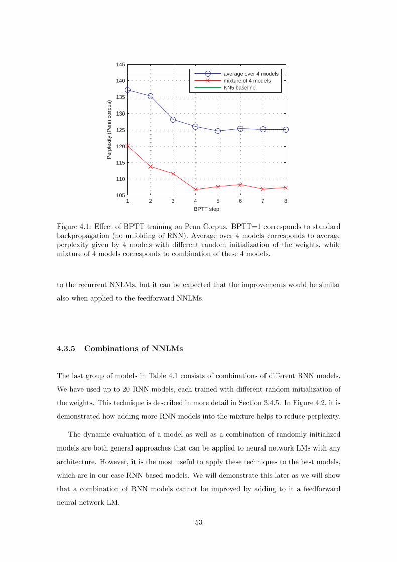
1 2 3 4 5 6 7 8105
110
115
120
125
130
135
140
145
BPTT step
Per
plex
ity (
Pen
n co
rpus
)
average over 4 modelsmixture of 4 modelsKN5 baseline
Figure 4.1: Effect of BPTT training on Penn Corpus. BPTT=1 corresponds to standardbackpropagation (no unfolding of RNN). Average over 4 models corresponds to averageperplexity given by 4 models with different random initialization of the weights, whilemixture of 4 models corresponds to combination of these 4 models.
to the recurrent NNLMs, but it can be expected that the improvements would be similar
also when applied to the feedforward NNLMs.
4.3.5 Combinations of NNLMs
The last group of models in Table 4.1 consists of combinations of different RNN models.
We have used up to 20 RNN models, each trained with different random initialization of
the weights. This technique is described in more detail in Section 3.4.5. In Figure 4.2, it is
demonstrated how adding more RNN models into the mixture helps to reduce perplexity.
The dynamic evaluation of a model as well as a combination of randomly initialized
models are both general approaches that can be applied to neural network LMs with any
architecture. However, it is the most useful to apply these techniques to the best models,
which are in our case RNN based models. We will demonstrate this later as we will show
that a combination of RNN models cannot be improved by adding to it a feedforward
neural network LM.
53
0 5 10 15 20 2595
100
105
110
115
120
125
130
Number of RNN models
Per
plex
ity (
Pen
n co
rpus
)
RNN mixtureRNN mixture + KN5
Figure 4.2: Linear interpolation of RNN models trained with different random initializa-tion of the weights.
4.4 Comparison of Different Neural Network Architectures
As neural network language models seem to work very well, we will describe them and
compare their performances in more detail. As can be seen in Table 4.1, the performance
of neural network based models with feedforward architectures is almost identical. The
syntactical NNLM has an advantage of having more input features: it uses a syntactical
parser to obtain part of speech tags for words in a sentence. We can observe that a signif-
icant improvement was obtained by using these additional features. On the other hand,
application of this technique to new languages and domains might not be straightforward,
as it relies on a syntactical parser that has to be trained on (usually) hand-annotated
data. There has been a following work done by Emami [22], where it is shown how differ-
ent linguistic features affect results, both perplexity and word error rate. The conclusion
of that experiments seems to be that the linguistic features improve only perplexity, but
do not reduce the word error rate.
Additional input features make interpretation of the results quite difficult: it can be
seen that the PTB corpus is quite small, and thus having additional information from a
parser that is trained on additional data (POS tags of words) can be a great boost to the
results. However, with increased amount of the training data, such additional information
would be probably less useful. Thus, it would be more convincing if the results obtained
54
with syntactical NNLMs would be presented on larger data sets, containing at least several
hundreds of millions of words.
The other way to improve accuracy of the model is to allow it to represent compactly
larger set of patterns. By changing the topology of the network from a feedforward to
a recurrent one, we allow the model to form a short context memory that is learned
unsupervisedly from the data. The prediction of the next word then depends on the
previous word and the state of the short context memory. We can thus claim that such
model can actually cluster entire histories that are in some sense similar. This is in
contrast to feedforward neural networks that can effectively cluster only individual words
in the projection layer, and then it is needed to perform another step to cluster the low-
dimensional representation of several words from the history. If some pattern involves
variable position of some word in the history, it is not possible to represent such pattern
efficiently with a compact feedforward network, while this can be accomplished by using
a recurrent one.
From the empirical point of view, we can see in Table 4.1 that recurrent networks
work both better than feedforward networks, and also better than feedforward networks
with additional linguistic features. A question arises, if this improvement does not come
from simply learning cache-like information from the data, as the recurrent topology ac-
tually allows this. Theoretical explanation from Bengio [4] shows that this actually can
not happen if RNN is trained by stochastic gradient descent, as the error signal that is
propagated through the recurrent connections converges to zero fast in most cases, thus
it is hard to train a recurrent network to represent long term patterns that would span
over several sentences. Table 4.1 shows empirical results, where we can see a combination
with a cache model: we can observe that in combination with the KN5+cache model the
recurrent network is behaving in a very similar way as the feedforward networks. Thus we
can conclude that the improvements obtained with RNN models come from better repre-
sentation of short context information, and not from learning cache information. Overall,
we can see 2.4% improvement in entropy when comparing the neural net with the feed-
forward achitecture (PPL 140.2) and with the recurrent achitecture (PPL 124.7). This is
a large improvement, especially if we consider that the feedforward neural network itself
has a very good position among studied models.
The dynamic evaluation of the RNN model provides further improvement. While
the perplexity reduction against the static RNN model is small, we will see in the next
55
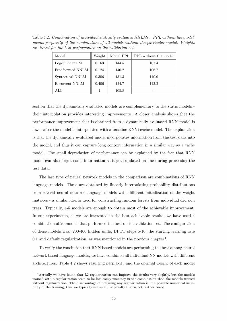
Table 4.2: Combination of individual statically evaluated NNLMs. ’PPL without the model’means perplexity of the combination of all models without the particular model. Weightsare tuned for the best performance on the validation set.
Model Weight Model PPL PPL without the model
Log-bilinear LM 0.163 144.5 107.4
Feedforward NNLM 0.124 140.2 106.7
Syntactical NNLM 0.306 131.3 110.9
Recurrent NNLM 0.406 124.7 113.2
ALL 1 105.8 -
section that the dynamically evaluated models are complementary to the static models -
their interpolation provides interesting improvements. A closer analysis shows that the
performance improvement that is obtained from a dynamically evaluated RNN model is
lower after the model is interpolated with a baseline KN5+cache model. The explanation
is that the dynamically evaluated model incorporates information from the test data into
the model, and thus it can capture long context information in a similar way as a cache
model. The small degradation of performance can be explained by the fact that RNN
model can also forget some information as it gets updated on-line during processing the
test data.
The last type of neural network models in the comparison are combinations of RNN
language models. These are obtained by linearly interpolating probability distributions
from several neural network language models with different initialization of the weight
matrices - a similar idea is used for constructing random forests from individual decision
trees. Typically, 4-5 models are enough to obtain most of the achievable improvement.
In our experiments, as we are interested in the best achievable results, we have used a
combination of 20 models that performed the best on the validation set. The configuration
of these models was: 200-400 hidden units, BPTT steps 5-10, the starting learning rate
0.1 and default regularization, as was mentioned in the previous chapter4.
To verify the conclusion that RNN based models are performing the best among neural
network based language models, we have combined all individual NN models with different
architectures. Table 4.2 shows resulting perplexity and the optimal weight of each model
4Actually we have found that L2 regularization can improve the results very slightly, but the modelstrained with a regularization seem to be less complementary in the combination than the models trainedwithout regularization. The disadvantage of not using any regularization is in a possible numerical insta-bility of the training, thus we typically use small L2 penalty that is not further tuned.
56
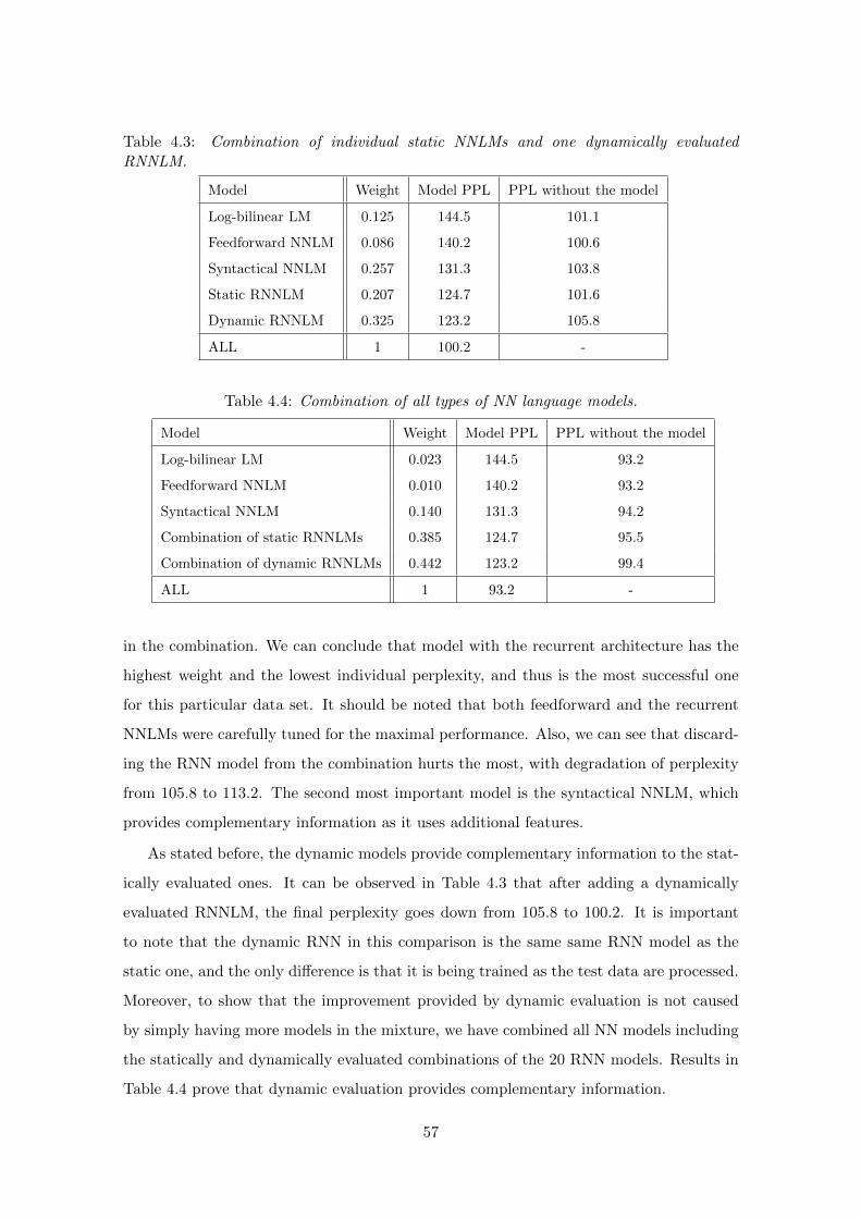
Table 4.3: Combination of individual static NNLMs and one dynamically evaluatedRNNLM.
Model Weight Model PPL PPL without the model
Log-bilinear LM 0.125 144.5 101.1
Feedforward NNLM 0.086 140.2 100.6
Syntactical NNLM 0.257 131.3 103.8
Static RNNLM 0.207 124.7 101.6
Dynamic RNNLM 0.325 123.2 105.8
ALL 1 100.2 -
Table 4.4: Combination of all types of NN language models.
Model Weight Model PPL PPL without the model
Log-bilinear LM 0.023 144.5 93.2
Feedforward NNLM 0.010 140.2 93.2
Syntactical NNLM 0.140 131.3 94.2
Combination of static RNNLMs 0.385 124.7 95.5
Combination of dynamic RNNLMs 0.442 123.2 99.4
ALL 1 93.2 -
in the combination. We can conclude that model with the recurrent architecture has the
highest weight and the lowest individual perplexity, and thus is the most successful one
for this particular data set. It should be noted that both feedforward and the recurrent
NNLMs were carefully tuned for the maximal performance. Also, we can see that discard-
ing the RNN model from the combination hurts the most, with degradation of perplexity
from 105.8 to 113.2. The second most important model is the syntactical NNLM, which
provides complementary information as it uses additional features.
As stated before, the dynamic models provide complementary information to the stat-
ically evaluated ones. It can be observed in Table 4.3 that after adding a dynamically
evaluated RNNLM, the final perplexity goes down from 105.8 to 100.2. It is important
to note that the dynamic RNN in this comparison is the same same RNN model as the
static one, and the only difference is that it is being trained as the test data are processed.
Moreover, to show that the improvement provided by dynamic evaluation is not caused
by simply having more models in the mixture, we have combined all NN models including
the statically and dynamically evaluated combinations of the 20 RNN models. Results in
Table 4.4 prove that dynamic evaluation provides complementary information.
57
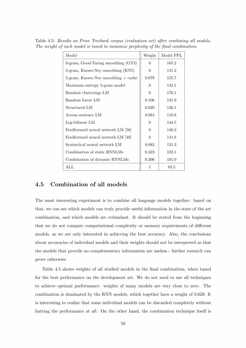
Table 4.5: Results on Penn Treebank corpus (evaluation set) after combining all models.The weight of each model is tuned to minimize perplexity of the final combination.
Model Weight Model PPL
3-gram, Good-Turing smoothing (GT3) 0 165.2
5-gram, Kneser-Ney smoothing (KN5) 0 141.2
5-gram, Kneser-Ney smoothing + cache 0.079 125.7
Maximum entropy 5-gram model 0 142.1
Random clusterings LM 0 170.1
Random forest LM 0.106 131.9
Structured LM 0.020 146.1
Across sentence LM 0.084 116.6
Log-bilinear LM 0 144.5
Feedforward neural network LM [50] 0 140.2
Feedforward neural network LM [40] 0 141.8
Syntactical neural network LM 0.083 131.3
Combination of static RNNLMs 0.323 102.1
Combination of dynamic RNNLMs 0.306 101.0
ALL 1 83.5
4.5 Combination of all models
The most interesting experiment is to combine all language models together: based on
that, we can see which models can truly provide useful information in the state of the art
combination, and which models are redundant. It should be stated from the beginning
that we do not compare computational complexity or memory requirements of different
models, as we are only interested in achieving the best accuracy. Also, the conclusions
about accuracies of individual models and their weights should not be interpreted as that
the models that provide no complementary information are useless - further research can
prove otherwise.
Table 4.5 shows weights of all studied models in the final combination, when tuned
for the best performance on the development set. We do not need to use all techniques
to achieve optimal performance: weights of many models are very close to zero. The
combination is dominated by the RNN models, which together have a weight of 0.629. It
is interesting to realize that some individual models can be discarded completely without
hurting the performance at all. On the other hand, the combination technique itself is
58
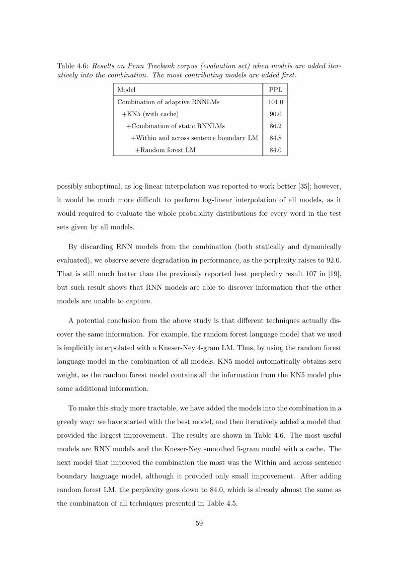
Table 4.6: Results on Penn Treebank corpus (evaluation set) when models are added iter-atively into the combination. The most contributing models are added first.
Model PPL
Combination of adaptive RNNLMs 101.0
+KN5 (with cache) 90.0
+Combination of static RNNLMs 86.2
+Within and across sentence boundary LM 84.8
+Random forest LM 84.0
possibly suboptimal, as log-linear interpolation was reported to work better [35]; however,
it would be much more difficult to perform log-linear interpolation of all models, as it
would required to evaluate the whole probability distributions for every word in the test
sets given by all models.
By discarding RNN models from the combination (both statically and dynamically
evaluated), we observe severe degradation in performance, as the perplexity raises to 92.0.
That is still much better than the previously reported best perplexity result 107 in [19],
but such result shows that RNN models are able to discover information that the other
models are unable to capture.
A potential conclusion from the above study is that different techniques actually dis-
cover the same information. For example, the random forest language model that we used
is implicitly interpolated with a Kneser-Ney 4-gram LM. Thus, by using the random forest
language model in the combination of all models, KN5 model automatically obtains zero
weight, as the random forest model contains all the information from the KN5 model plus
some additional information.
To make this study more tractable, we have added the models into the combination in a
greedy way: we have started with the best model, and then iteratively added a model that
provided the largest improvement. The results are shown in Table 4.6. The most useful
models are RNN models and the Kneser-Ney smoothed 5-gram model with a cache. The
next model that improved the combination the most was the Within and across sentence
boundary language model, although it provided only small improvement. After adding
random forest LM, the perplexity goes down to 84.0, which is already almost the same as
the combination of all techniques presented in Table 4.5.
59
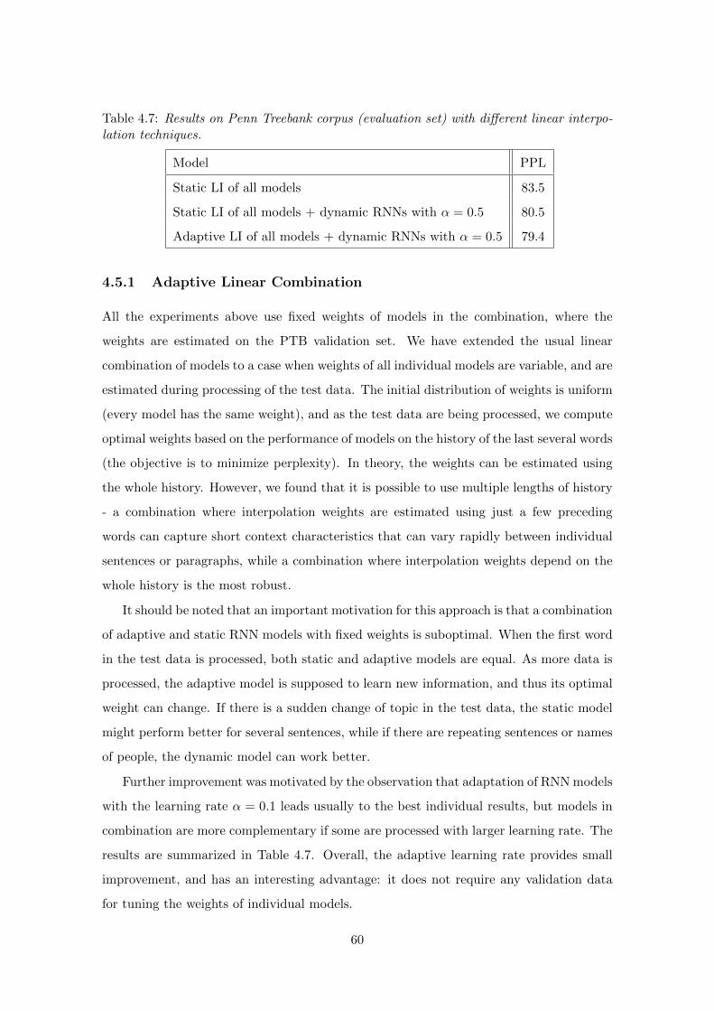
Table 4.7: Results on Penn Treebank corpus (evaluation set) with different linear interpo-lation techniques.
Model PPL
Static LI of all models 83.5
Static LI of all models + dynamic RNNs with α = 0.5 80.5
Adaptive LI of all models + dynamic RNNs with α = 0.5 79.4
4.5.1 Adaptive Linear Combination
All the experiments above use fixed weights of models in the combination, where the
weights are estimated on the PTB validation set. We have extended the usual linear
combination of models to a case when weights of all individual models are variable, and are
estimated during processing of the test data. The initial distribution of weights is uniform
(every model has the same weight), and as the test data are being processed, we compute
optimal weights based on the performance of models on the history of the last several words
(the objective is to minimize perplexity). In theory, the weights can be estimated using
the whole history. However, we found that it is possible to use multiple lengths of history
- a combination where interpolation weights are estimated using just a few preceding
words can capture short context characteristics that can vary rapidly between individual
sentences or paragraphs, while a combination where interpolation weights depend on the
whole history is the most robust.
It should be noted that an important motivation for this approach is that a combination
of adaptive and static RNN models with fixed weights is suboptimal. When the first word
in the test data is processed, both static and adaptive models are equal. As more data is
processed, the adaptive model is supposed to learn new information, and thus its optimal
weight can change. If there is a sudden change of topic in the test data, the static model
might perform better for several sentences, while if there are repeating sentences or names
of people, the dynamic model can work better.
Further improvement was motivated by the observation that adaptation of RNN models
with the learning rate α = 0.1 leads usually to the best individual results, but models in
combination are more complementary if some are processed with larger learning rate. The
results are summarized in Table 4.7. Overall, the adaptive learning rate provides small
improvement, and has an interesting advantage: it does not require any validation data
for tuning the weights of individual models.
60
4.6 Conclusion of the Model Combination Experiments
We have achieved a new state of the art results on the well-known Penn Treebank Corpus,
as we reduced the perplexity from the baseline 141.2 to 83.5 by combining many advanced
language modeling techniques. Perplexity was further reduced to 79.4 by using adaptive
linear interpolation of models and by using larger learning rate for dynamic RNN models.
These experiments were already described in [51].
In the subsequent experiments, we were able to obtain perplexity 78.8 by using
in the model combination also RNNME models that will be described in the Chapter 6.
This corresponds to 11.8% reduction of entropy over 5-gram model with modified
Kneser-Ney smoothing and no count cutoffs - this is more than twice more entropy
reduction than the best previously published result on the Penn Treebank data set.
It is quite important and interesting to realize that we can actually rely just on a
few techniques to reach near-optimal performance. Combination of RNNLMs and KN5
model with a cache is very simple and straightforward. All these techniques are purely
data driven, with no need for extra domain knowledge. This is in contrast to techniques
that rely for example on syntactical parsers, which require human-annotated data. Thus,
my conclusion for the experiments with the Penn Treebank corpus is that techniques that
focus on the modeling outperform techniques that focus on the features and attempt to
incorporate knowledge provided by human experts. This might suggest that the task of
learning the language should focus more on the learning itself, than on hand-designing
features and complex models by linguists. I believe that systems that rely on the extra
information provided by humans may be useful in the short term perspective, but from
the long term one, the machine learning algorithms will improve and overcome the rule
based systems, as there is a great availability of unstructured data. Just by looking at
the evolution of the speech recognition field, it is possible to observe this drift towards
statistical learning. Interestingly, also the research scientists from big companies such as
Google claim that systems without special linguistic features work if not the same, then
even better [58].
61
Chapter 5
Wall Street Journal Experiments
Another important data set frequently used by the speech recognition community for
research purposes is the Wall Street Journal speech recognition task. In the following
experiments, we aim to:
• show full potential of RNN LMs on moderately sized task, where speech recognition
errors are mainly caused by the language model (as opposed to acoustically noisy
tasks where it would be more important to work on the acoustic models)
• show performance of RNN LMs with increasing amount of the training data
• provide comparison to other advanced language modeling techniques in terms of
word error rate
• describe experiments with open source speech recognition toolkit Kaldi that can be
reproduced
5.1 WSJ-JHU Setup Description
The experiments in this section were performed with data set that was kindly shared
with us by researchers from Johns Hopkins university. We report results after rescoring
100-best lists from DARPA WSJ’92 and WSJ’93 data sets - the same data sets were used
by Xu [79], Filimonov [23], and in my previous work [49]. Oracle WER of the 100-best
lists is 6.1% for the development set and 9.5% for the evaluation set. Training data for
the language model are the same as used by Xu [79]. The training corpus consists of 37M
words from NYT section of English Gigaword. The hyper-parameters for all RNN models
62
were: 400 classes, hidden layer size up to 800 neurons. Other hyper-parameters such as
interpolation weights were tuned on the WSJ’92 set (333 sentences), and the WSJ’93 set
used for evaluation consists of 465 sentences.
Note that this setup is very simple as the acoustic models that were used to generate
n-best lists for this task were not the state of the art. Also, the corresponding language
models used in the previous research were trained just on limited amount of the training
data (37M-70M words), although by using more training data that are easily affordable
for this task, better performance can be expected. The same holds for the vocabulary - a
20K word list was used, although it would be simple to use more. Thus, the experiments
on this setup are not supposed to beat the state of the art, but to allow comparison to
other LM techniques and to provide more insight into the performance of the RNN LMs.
5.1.1 Results on the JHU Setup
Results with RNN models and competitive techniques are summarized in Table 5.1. The
best RNN models have very high optimal weight when combined with KN5 baseline model,
and actually by discarding the n-gram model completely, the results are not significantly
affected. Interpolation of three RNN models gives the best results - the word error rate
is reduced relatively by about 20%. Other techniques, such as discriminatively trained
language model and joint LM (structured model) provide smaller improvements, only
about 2-3% reduction of WER on the evaluation set.
The adapted RNN model is not evaluated as a dynamic RNN LM described in the
previous chapters, but simply a static model that is re-trained on the 1-best lists. This was
done due to performance issues; it becomes relatively slow to work with RNN models that
are continuously updated, especially in the n-best list rescoring framework. Adaptation
itself provides relatively small improvement, especially with the large models.
5.1.2 Performance with Increasing Size of the Training Data
It was observed by Joshua Goodman that with increasing amount of the training data,
improvements provided by many advanced language modeling techniques vanish, with
a possible conclusion that it might be sufficient to train basic n-gram models on huge
amounts of data to obtain good performance [24]. This is sometimes interpreted as an
argument against language modeling research; however, as was mentioned in the introduc-
tion of this thesis, simple counting of words in different contexts is far from being close
63
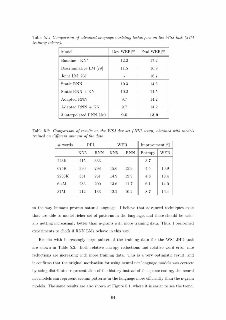
Table 5.1: Comparison of advanced language modeling techniques on the WSJ task (37Mtraining tokens).
Model Dev WER[%] Eval WER[%]
Baseline - KN5 12.2 17.2
Discriminative LM [79] 11.5 16.9
Joint LM [23] - 16.7
Static RNN 10.3 14.5
Static RNN + KN 10.2 14.5
Adapted RNN 9.7 14.2
Adapted RNN + KN 9.7 14.2
3 interpolated RNN LMs 9.5 13.9
Table 5.2: Comparison of results on the WSJ dev set (JHU setup) obtained with modelstrained on different amount of the data.
# words PPL WER Improvement[%]
KN5 +RNN KN5 +RNN Entropy WER
223K 415 333 - - 3.7 -
675K 390 298 15.6 13.9 4.5 10.9
2233K 331 251 14.9 12.9 4.8 13.4
6.4M 283 200 13.6 11.7 6.1 14.0
37M 212 133 12.2 10.2 8.7 16.4
to the way humans process natural language. I believe that advanced techniques exist
that are able to model richer set of patterns in the language, and these should be actu-
ally getting increasingly better than n-grams with more training data. Thus, I performed
experiments to check if RNN LMs behave in this way.
Results with increasingly large subset of the training data for the WSJ-JHU task
are shown in Table 5.2. Both relative entropy reductions and relative word error rate
reductions are increasing with more training data. This is a very optimistic result, and
it confirms that the original motivation for using neural net language models was correct:
by using distributed representation of the history instead of the sparse coding, the neural
net models can represent certain patterns in the language more efficiently than the n-gram
models. The same results are also shown at Figure 5.1, where it is easier to see the trend.
64
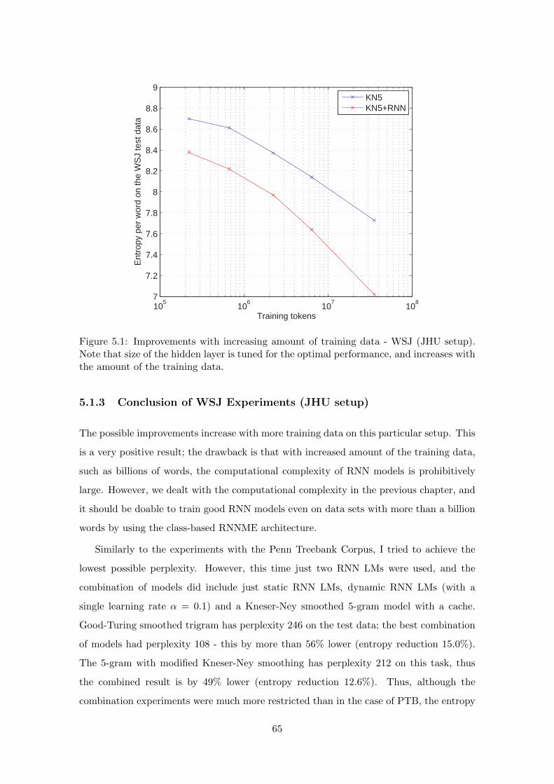
105
106
107
108
7
7.2
7.4
7.6
7.8
8
8.2
8.4
8.6
8.8
9
Training tokens
Ent
ropy
per
wor
d on
the
WS
J te
st d
ata
KN5KN5+RNN
Figure 5.1: Improvements with increasing amount of training data - WSJ (JHU setup).Note that size of the hidden layer is tuned for the optimal performance, and increases withthe amount of the training data.
5.1.3 Conclusion of WSJ Experiments (JHU setup)
The possible improvements increase with more training data on this particular setup. This
is a very positive result; the drawback is that with increased amount of the training data,
such as billions of words, the computational complexity of RNN models is prohibitively
large. However, we dealt with the computational complexity in the previous chapter, and
it should be doable to train good RNN models even on data sets with more than a billion
words by using the class-based RNNME architecture.
Similarly to the experiments with the Penn Treebank Corpus, I tried to achieve the
lowest possible perplexity. However, this time just two RNN LMs were used, and the
combination of models did include just static RNN LMs, dynamic RNN LMs (with a
single learning rate α = 0.1) and a Kneser-Ney smoothed 5-gram model with a cache.
Good-Turing smoothed trigram has perplexity 246 on the test data; the best combination
of models had perplexity 108 - this by more than 56% lower (entropy reduction 15.0%).
The 5-gram with modified Kneser-Ney smoothing has perplexity 212 on this task, thus
the combined result is by 49% lower (entropy reduction 12.6%). Thus, although the
combination experiments were much more restricted than in the case of PTB, the entropy
65
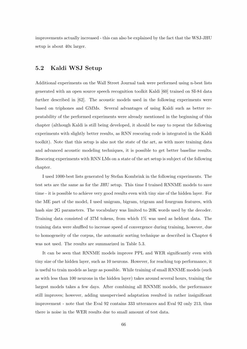
improvements actually increased - this can also be explained by the fact that the WSJ-JHU
setup is about 40x larger.
5.2 Kaldi WSJ Setup
Additional experiments on the Wall Street Journal task were performed using n-best lists
generated with an open source speech recognition toolkit Kaldi [60] trained on SI-84 data
further described in [62]. The acoustic models used in the following experiments were
based on triphones and GMMs. Several advantages of using Kaldi such as better re-
peatability of the performed experiments were already mentioned in the beginning of this
chapter (although Kaldi is still being developed, it should be easy to repeat the following
experiments with slightly better results, as RNN rescoring code is integrated in the Kaldi
toolkit). Note that this setup is also not the state of the art, as with more training data
and advanced acoustic modeling techniques, it is possible to get better baseline results.
Rescoring experiments with RNN LMs on a state of the art setup is subject of the following
chapter.
I used 1000-best lists generated by Stefan Kombrink in the following experiments. The
test sets are the same as for the JHU setup. This time I trained RNNME models to save
time - it is possible to achieve very good results even with tiny size of the hidden layer. For
the ME part of the model, I used unigram, bigram, trigram and fourgram features, with
hash size 2G parameters. The vocabulary was limited to 20K words used by the decoder.
Training data consisted of 37M tokens, from which 1% was used as heldout data. The
training data were shuffled to increase speed of convergence during training, however, due
to homogeneity of the corpus, the automatic sorting technique as described in Chapter 6
was not used. The results are summarized in Table 5.3.
It can be seen that RNNME models improve PPL and WER significantly even with
tiny size of the hidden layer, such as 10 neurons. However, for reaching top performance, it
is useful to train models as large as possible. While training of small RNNME models (such
as with less than 100 neurons in the hidden layer) takes around several hours, training the
largest models takes a few days. After combining all RNNME models, the performance
still improves; however, adding unsupervised adaptation resulted in rather insignificant
improvement - note that the Eval 92 contains 333 utterances and Eval 92 only 213, thus
there is noise in the WER results due to small amount of test data.
66
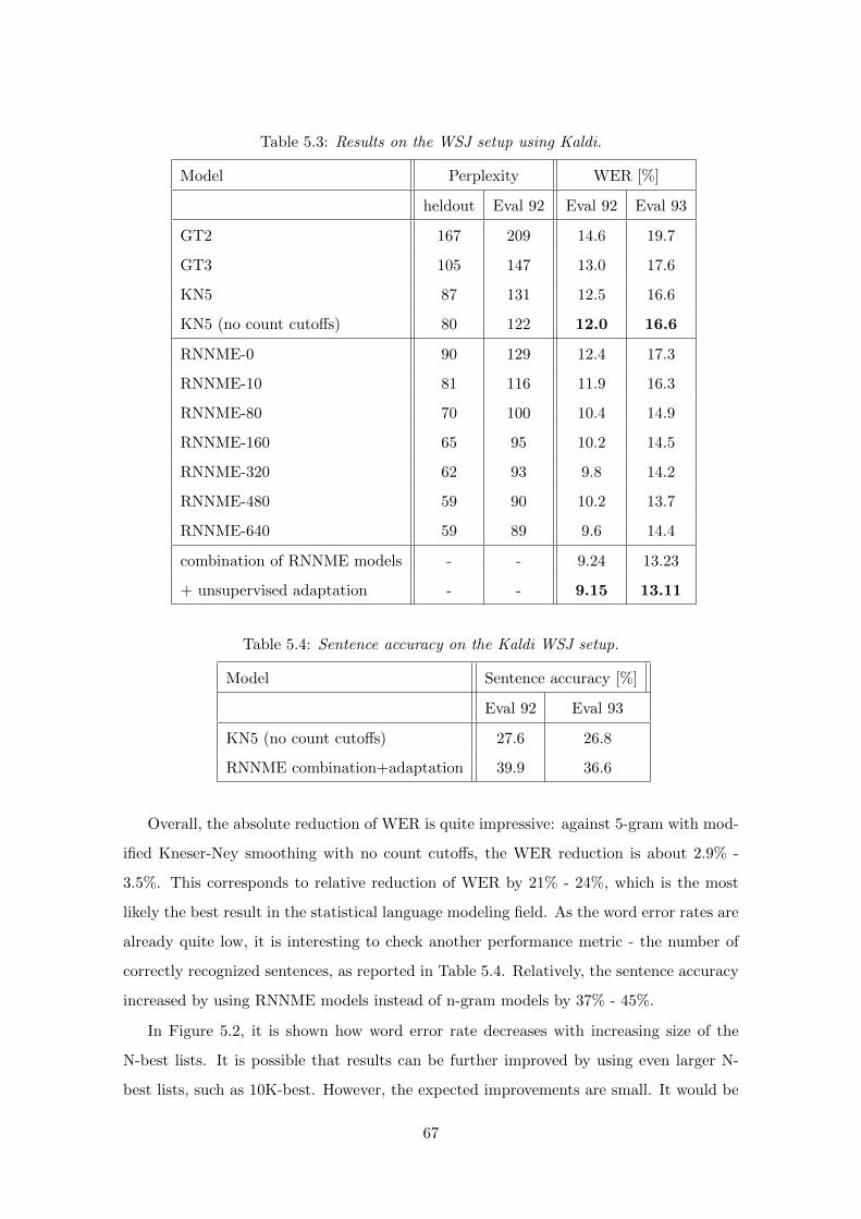
Table 5.3: Results on the WSJ setup using Kaldi.
Model Perplexity WER [%]
heldout Eval 92 Eval 92 Eval 93
GT2 167 209 14.6 19.7
GT3 105 147 13.0 17.6
KN5 87 131 12.5 16.6
KN5 (no count cutoffs) 80 122 12.0 16.6
RNNME-0 90 129 12.4 17.3
RNNME-10 81 116 11.9 16.3
RNNME-80 70 100 10.4 14.9
RNNME-160 65 95 10.2 14.5
RNNME-320 62 93 9.8 14.2
RNNME-480 59 90 10.2 13.7
RNNME-640 59 89 9.6 14.4
combination of RNNME models - - 9.24 13.23
+ unsupervised adaptation - - 9.15 13.11
Table 5.4: Sentence accuracy on the Kaldi WSJ setup.
Model Sentence accuracy [%]
Eval 92 Eval 93
KN5 (no count cutoffs) 27.6 26.8
RNNME combination+adaptation 39.9 36.6
Overall, the absolute reduction of WER is quite impressive: against 5-gram with mod-
ified Kneser-Ney smoothing with no count cutoffs, the WER reduction is about 2.9% -
3.5%. This corresponds to relative reduction of WER by 21% - 24%, which is the most
likely the best result in the statistical language modeling field. As the word error rates are
already quite low, it is interesting to check another performance metric - the number of
correctly recognized sentences, as reported in Table 5.4. Relatively, the sentence accuracy
increased by using RNNME models instead of n-gram models by 37% - 45%.
In Figure 5.2, it is shown how word error rate decreases with increasing size of the
N-best lists. It is possible that results can be further improved by using even larger N-
best lists, such as 10K-best. However, the expected improvements are small. It would be
67
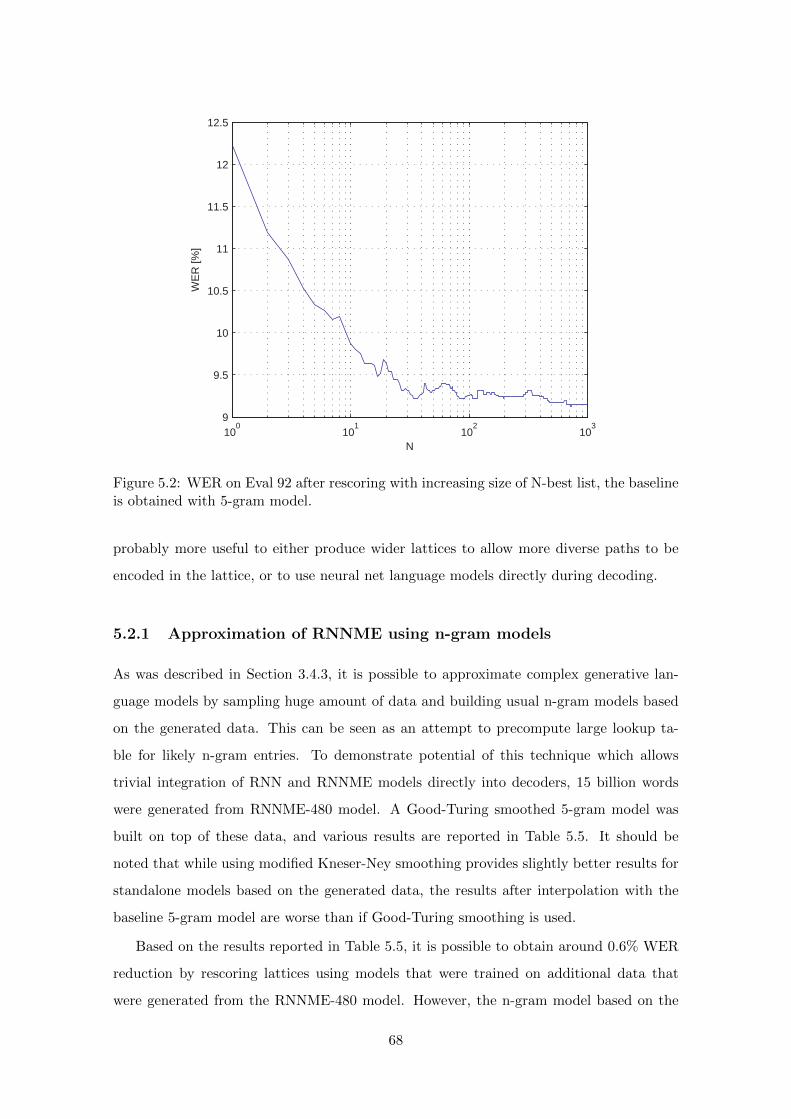
100
101
102
103
9
9.5
10
10.5
11
11.5
12
12.5
N
WE
R [%
]
Figure 5.2: WER on Eval 92 after rescoring with increasing size of N-best list, the baselineis obtained with 5-gram model.
probably more useful to either produce wider lattices to allow more diverse paths to be
encoded in the lattice, or to use neural net language models directly during decoding.
5.2.1 Approximation of RNNME using n-gram models
As was described in Section 3.4.3, it is possible to approximate complex generative lan-
guage models by sampling huge amount of data and building usual n-gram models based
on the generated data. This can be seen as an attempt to precompute large lookup ta-
ble for likely n-gram entries. To demonstrate potential of this technique which allows
trivial integration of RNN and RNNME models directly into decoders, 15 billion words
were generated from RNNME-480 model. A Good-Turing smoothed 5-gram model was
built on top of these data, and various results are reported in Table 5.5. It should be
noted that while using modified Kneser-Ney smoothing provides slightly better results for
standalone models based on the generated data, the results after interpolation with the
baseline 5-gram model are worse than if Good-Turing smoothing is used.
Based on the results reported in Table 5.5, it is possible to obtain around 0.6% WER
reduction by rescoring lattices using models that were trained on additional data that
were generated from the RNNME-480 model. However, the n-gram model based on the
68
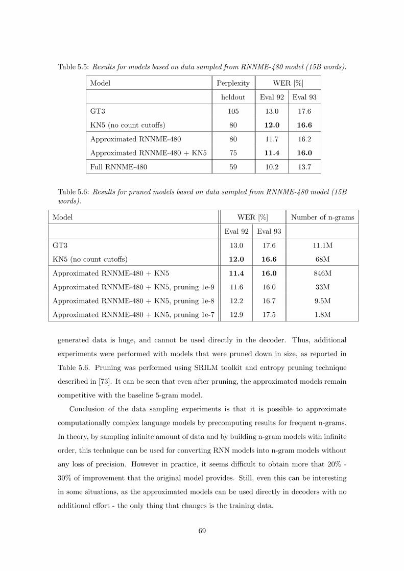
Table 5.5: Results for models based on data sampled from RNNME-480 model (15B words).
Model Perplexity WER [%]
heldout Eval 92 Eval 93
GT3 105 13.0 17.6
KN5 (no count cutoffs) 80 12.0 16.6
Approximated RNNME-480 80 11.7 16.2
Approximated RNNME-480 + KN5 75 11.4 16.0
Full RNNME-480 59 10.2 13.7
Table 5.6: Results for pruned models based on data sampled from RNNME-480 model (15Bwords).
Model WER [%] Number of n-grams
Eval 92 Eval 93
GT3 13.0 17.6 11.1M
KN5 (no count cutoffs) 12.0 16.6 68M
Approximated RNNME-480 + KN5 11.4 16.0 846M
Approximated RNNME-480 + KN5, pruning 1e-9 11.6 16.0 33M
Approximated RNNME-480 + KN5, pruning 1e-8 12.2 16.7 9.5M
Approximated RNNME-480 + KN5, pruning 1e-7 12.9 17.5 1.8M
generated data is huge, and cannot be used directly in the decoder. Thus, additional
experiments were performed with models that were pruned down in size, as reported in
Table 5.6. Pruning was performed using SRILM toolkit and entropy pruning technique
described in [73]. It can be seen that even after pruning, the approximated models remain
competitive with the baseline 5-gram model.
Conclusion of the data sampling experiments is that it is possible to approximate
computationally complex language models by precomputing results for frequent n-grams.
In theory, by sampling infinite amount of data and by building n-gram models with infinite
order, this technique can be used for converting RNN models into n-gram models without
any loss of precision. However in practice, it seems difficult to obtain more that 20% -
30% of improvement that the original model provides. Still, even this can be interesting
in some situations, as the approximated models can be used directly in decoders with no
additional effort - the only thing that changes is the training data.
69
Chapter 6
Strategies for Training Large Scale
Neural Network Language Models
The experiments on the Penn Treebank Corpus have shown that mixtures of recurrent
neural networks trained by backpropagation through time provide state of the art results
in the field of statistical language modeling. However a remaining question is, if the
performance would be also this good with much larger amount of the training data -
the PTB corpus with about 1M training tokens can be considered as very small, because
language models are typically trained on corpora with orders of magnitude more data.
It is not unusual to work with huge training corpora that consist of much more than a
billion words. While application to low resource domains (especially for new languages
and for domains where only small amount of relevant data exists) is also a very interesting
research problem, the most convincing results are those obtained with well tuned state of
the art systems, which are trained on large amounts of data.
The experiments in the previous chapter focused on obtaining the largest possible
improvement, however some of the approaches would become computationally difficult
to apply to large data sets. In this chapter, we briefly mention existing approaches for
reducing the computational complexity of neural net language models (most of these ap-
proaches are also applicable to maximum entropy language models). We propose two new
simple techniques that can be used to reduce computational complexity of the training
and the test phases. We show that these new techniques are complementary to existing
approaches.
Most interestingly, we show that a standard neural network language model can be
70
trained together with a maximum entropy model, which can be seen as a part of the the
neural network, where the input layer is directly connected to the output layer. We intro-
duce a hash-based implementation of a class-based maximum entropy model, that allows
us to easily control the trade-off between the memory complexity, the space complexity
and the computational complexity.
In this chapter, we report results on the NIST RT04 Broadcast News speech recogni-
tion task. We use lattices generated from IBM Attila decoder [71] that uses state of the art
discriminatively trained acoustic models1. The language models for this task are trained
on about 400M tokens. This highly competitive setup has been used in the 2010 Speech
Recognition with Segmental Conditional Random Fields summer workshop at Johns Hop-
kins University2 [82]. Some of the results reported in this chapter were recently published
in [52].
6.1 Model Description
In this section, we will show that a maximum entropy model can be seen as a neural
network model with no hidden layer. A maximum entropy model has the following form:
P (w|h) =e∑N
i=1 λifi(h,w)∑w e
∑Ni=1 λifi(h,w)
, (6.1)
where f is a set of features, λ is a set of weights and h is a history. Training of maximum
entropy model consists of learning the set of weights λ. Usual features are n-grams, but it
is easy to integrate any information source into the model, for example triggers or syntactic
features [64]. The choice of features is usually done manually, and significantly affects the
overall performance of the model.
The standard neural network language model has a very similar form. The main
difference is that the features for this model are automatically learned as a function of
the history. Also, the usual features for the ME model are binary, while NN models use
continuous-valued features. We can describe the NN LM as follows:
P (w|h) =e∑N
i=1 λifi(s,w)∑w e
∑Ni=1 λifi(s,w)
, (6.2)
1The lattice rescoring experiments reported in this chapter were performed by Anoop Deoras at JHUdue to the license issues of the IBM recognizer.
2www.clsp.jhu.edu/workshops/archive/ws10/groups/speech-recognition-with-segmental-conditional-random-fields/
71
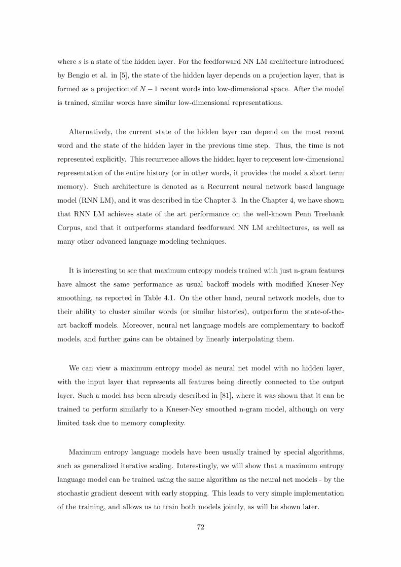
where s is a state of the hidden layer. For the feedforward NN LM architecture introduced
by Bengio et al. in [5], the state of the hidden layer depends on a projection layer, that is
formed as a projection of N − 1 recent words into low-dimensional space. After the model
is trained, similar words have similar low-dimensional representations.
Alternatively, the current state of the hidden layer can depend on the most recent
word and the state of the hidden layer in the previous time step. Thus, the time is not
represented explicitly. This recurrence allows the hidden layer to represent low-dimensional
representation of the entire history (or in other words, it provides the model a short term
memory). Such architecture is denoted as a Recurrent neural network based language
model (RNN LM), and it was described in the Chapter 3. In the Chapter 4, we have shown
that RNN LM achieves state of the art performance on the well-known Penn Treebank
Corpus, and that it outperforms standard feedforward NN LM architectures, as well as
many other advanced language modeling techniques.
It is interesting to see that maximum entropy models trained with just n-gram features
have almost the same performance as usual backoff models with modified Kneser-Ney
smoothing, as reported in Table 4.1. On the other hand, neural network models, due to
their ability to cluster similar words (or similar histories), outperform the state-of-the-
art backoff models. Moreover, neural net language models are complementary to backoff
models, and further gains can be obtained by linearly interpolating them.
We can view a maximum entropy model as neural net model with no hidden layer,
with the input layer that represents all features being directly connected to the output
layer. Such a model has been already described in [81], where it was shown that it can be
trained to perform similarly to a Kneser-Ney smoothed n-gram model, although on very
limited task due to memory complexity.
Maximum entropy language models have been usually trained by special algorithms,
such as generalized iterative scaling. Interestingly, we will show that a maximum entropy
language model can be trained using the same algorithm as the neural net models - by the
stochastic gradient descent with early stopping. This leads to very simple implementation
of the training, and allows us to train both models jointly, as will be shown later.
72
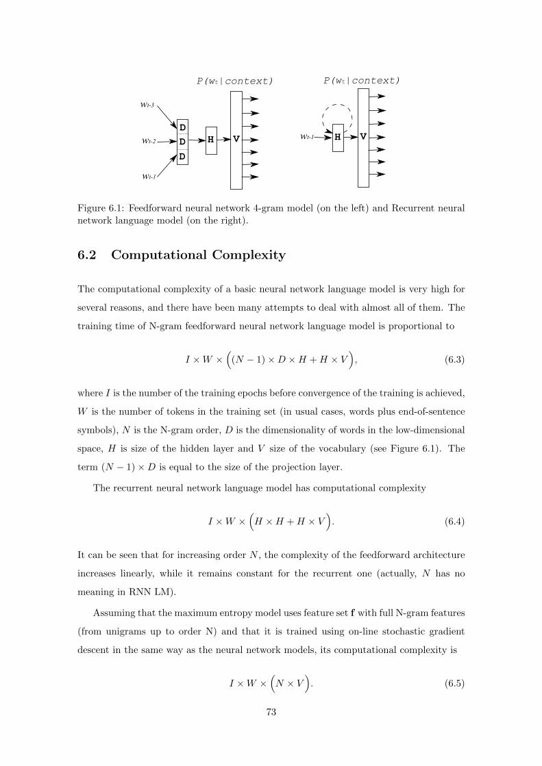
VH
D
D
DVHwt-1
wt-3
wt-1
wt-2
P(wt|context) P(wt|context)
Figure 6.1: Feedforward neural network 4-gram model (on the left) and Recurrent neuralnetwork language model (on the right).
6.2 Computational Complexity
The computational complexity of a basic neural network language model is very high for
several reasons, and there have been many attempts to deal with almost all of them. The
training time of N-gram feedforward neural network language model is proportional to
I ×W ×(
(N − 1)×D ×H +H × V), (6.3)
where I is the number of the training epochs before convergence of the training is achieved,
W is the number of tokens in the training set (in usual cases, words plus end-of-sentence
symbols), N is the N-gram order, D is the dimensionality of words in the low-dimensional
space, H is size of the hidden layer and V size of the vocabulary (see Figure 6.1). The
term (N − 1)×D is equal to the size of the projection layer.
The recurrent neural network language model has computational complexity
I ×W ×(H ×H +H × V
). (6.4)
It can be seen that for increasing order N , the complexity of the feedforward architecture
increases linearly, while it remains constant for the recurrent one (actually, N has no
meaning in RNN LM).
Assuming that the maximum entropy model uses feature set f with full N-gram features
(from unigrams up to order N) and that it is trained using on-line stochastic gradient
descent in the same way as the neural network models, its computational complexity is
I ×W ×(N × V
). (6.5)
73
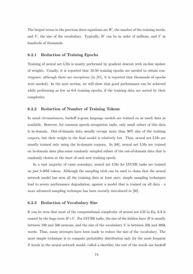
The largest terms in the previous three equations are W , the number of the training words,
and V , the size of the vocabulary. Typically, W can be in order of millions, and V in
hundreds of thousands.
6.2.1 Reduction of Training Epochs
Training of neural net LMs is mostly performed by gradient descent with on-line update
of weights. Usually, it is reported that 10-50 training epochs are needed to obtain con-
vergence, although there are exceptions (in [81], it is reported that thousands of epochs
were needed). In the next section, we will show that good performance can be achieved
while performing as few as 6-8 training epochs, if the training data are sorted by their
complexity.
6.2.2 Reduction of Number of Training Tokens
In usual circumstances, backoff n-gram language models are trained on as much data as
available. However, for common speech recognition tasks, only small subset of this data
is in-domain. Out-of-domain data usually occupy more than 90% size of the training
corpora, but their weight in the final model is relatively low. Thus, neural net LMs are
usually trained only using the in-domain corpora. In [68], neural net LMs are trained
on in-domain data plus some randomly sampled subset of the out-of-domain data that is
randomly chosen at the start of each new training epoch.
In a vast majority of cases nowadays, neural net LMs for LVCSR tasks are trained
on just 5-30M tokens. Although the sampling trick can be used to claim that the neural
network model has seen all the training data at least once, simple sampling techniques
lead to severe performance degradation, against a model that is trained on all data - a
more advanced sampling technique has been recently introduced in [80].
6.2.3 Reduction of Vocabulary Size
It can be seen that most of the computational complexity of neural net LM in Eq. 6.3 is
caused by the huge term H×V . For LVCSR tasks, the size of the hidden layer H is usually
between 100 and 500 neurons, and the size of the vocabulary V is between 50k and 300k
words. Thus, many attempts have been made to reduce the size of the vocabulary. The
most simple technique is to compute probability distribution only for the most frequent
S words in the neural network model, called a shortlist; the rest of the words use backoff
74
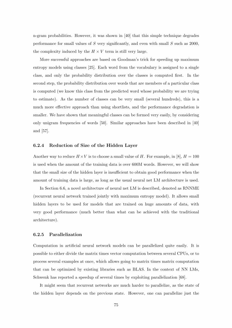
n-gram probabilities. However, it was shown in [40] that this simple technique degrades
performance for small values of S very significantly, and even with small S such as 2000,
the complexity induced by the H × V term is still very large.
More successful approaches are based on Goodman’s trick for speeding up maximum
entropy models using classes [25]. Each word from the vocabulary is assigned to a single
class, and only the probability distribution over the classes is computed first. In the
second step, the probability distribution over words that are members of a particular class
is computed (we know this class from the predicted word whose probability we are trying
to estimate). As the number of classes can be very small (several hundreds), this is a
much more effective approach than using shortlists, and the performance degradation is
smaller. We have shown that meaningful classes can be formed very easily, by considering
only unigram frequencies of words [50]. Similar approaches have been described in [40]
and [57].
6.2.4 Reduction of Size of the Hidden Layer
Another way to reduce H×V is to choose a small value of H. For example, in [8], H = 100
is used when the amount of the training data is over 600M words. However, we will show
that the small size of the hidden layer is insufficient to obtain good performance when the
amount of training data is large, as long as the usual neural net LM architecture is used.
In Section 6.6, a novel architecture of neural net LM is described, denoted as RNNME
(recurrent neural network trained jointly with maximum entropy model). It allows small
hidden layers to be used for models that are trained on huge amounts of data, with
very good performance (much better than what can be achieved with the traditional
architecture).
6.2.5 Parallelization
Computation in artificial neural network models can be parallelized quite easily. It is
possible to either divide the matrix times vector computation between several CPUs, or to
process several examples at once, which allows going to matrix times matrix computation
that can be optimized by existing libraries such as BLAS. In the context of NN LMs,
Schwenk has reported a speedup of several times by exploiting parallelization [68].
It might seem that recurrent networks are much harder to parallelize, as the state of
the hidden layer depends on the previous state. However, one can parallelize just the
75
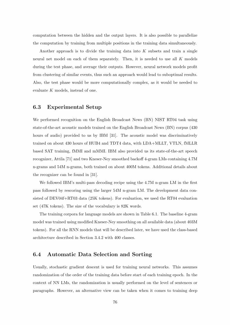
computation between the hidden and the output layers. It is also possible to parallelize
the computation by training from multiple positions in the training data simultaneously.
Another approach is to divide the training data into K subsets and train a single
neural net model on each of them separately. Then, it is needed to use all K models
during the test phase, and average their outputs. However, neural network models profit
from clustering of similar events, thus such an approach would lead to suboptimal results.
Also, the test phase would be more computationally complex, as it would be needed to
evaluate K models, instead of one.
6.3 Experimental Setup
We performed recognition on the English Broadcast News (BN) NIST RT04 task using
state-of-the-art acoustic models trained on the English Broadcast News (BN) corpus (430
hours of audio) provided to us by IBM [31]. The acoustic model was discriminatively
trained on about 430 hours of HUB4 and TDT4 data, with LDA+MLLT, VTLN, fMLLR
based SAT training, fMMI and mMMI. IBM also provided us its state-of-the-art speech
recognizer, Attila [71] and two Kneser-Ney smoothed backoff 4-gram LMs containing 4.7M
n-grams and 54M n-grams, both trained on about 400M tokens. Additional details about
the recognizer can be found in [31].
We followed IBM’s multi-pass decoding recipe using the 4.7M n-gram LM in the first
pass followed by rescoring using the larger 54M n-gram LM. The development data con-
sisted of DEV04f+RT03 data (25K tokens). For evaluation, we used the RT04 evaluation
set (47K tokens). The size of the vocabulary is 82K words.
The training corpora for language models are shown in Table 6.1. The baseline 4-gram
model was trained using modified Kneser-Ney smoothing on all available data (about 403M
tokens). For all the RNN models that will be described later, we have used the class-based
architecture described in Section 3.4.2 with 400 classes.
6.4 Automatic Data Selection and Sorting
Usually, stochastic gradient descent is used for training neural networks. This assumes
randomization of the order of the training data before start of each training epoch. In the
context of NN LMs, the randomization is usually performed on the level of sentences or
paragraphs. However, an alternative view can be taken when it comes to training deep
76
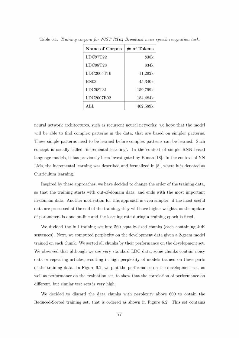
Table 6.1: Training corpora for NIST RT04 Broadcast news speech recognition task.
Name of Corpus # of Tokens
LDC97T22 838k
LDC98T28 834k
LDC2005T16 11,292k
BN03 45,340k
LDC98T31 159,799k
LDC2007E02 184,484k
ALL 402,589k
neural network architectures, such as recurrent neural networks: we hope that the model
will be able to find complex patterns in the data, that are based on simpler patterns.
These simple patterns need to be learned before complex patterns can be learned. Such
concept is usually called ‘incremental learning’. In the context of simple RNN based
language models, it has previously been investigated by Elman [18]. In the context of NN
LMs, the incremental learning was described and formalized in [8], where it is denoted as
Curriculum learning.
Inspired by these approaches, we have decided to change the order of the training data,
so that the training starts with out-of-domain data, and ends with the most important
in-domain data. Another motivation for this approach is even simpler: if the most useful
data are processed at the end of the training, they will have higher weights, as the update
of parameters is done on-line and the learning rate during a training epoch is fixed.
We divided the full training set into 560 equally-sized chunks (each containing 40K
sentences). Next, we computed perplexity on the development data given a 2-gram model
trained on each chunk. We sorted all chunks by their performance on the development set.
We observed that although we use very standard LDC data, some chunks contain noisy
data or repeating articles, resulting in high perplexity of models trained on these parts
of the training data. In Figure 6.2, we plot the performance on the development set, as
well as performance on the evaluation set, to show that the correlation of performance on
different, but similar test sets is very high.
We decided to discard the data chunks with perplexity above 600 to obtain the
Reduced-Sorted training set, that is ordered as shown in Figure 6.2. This set contains
77
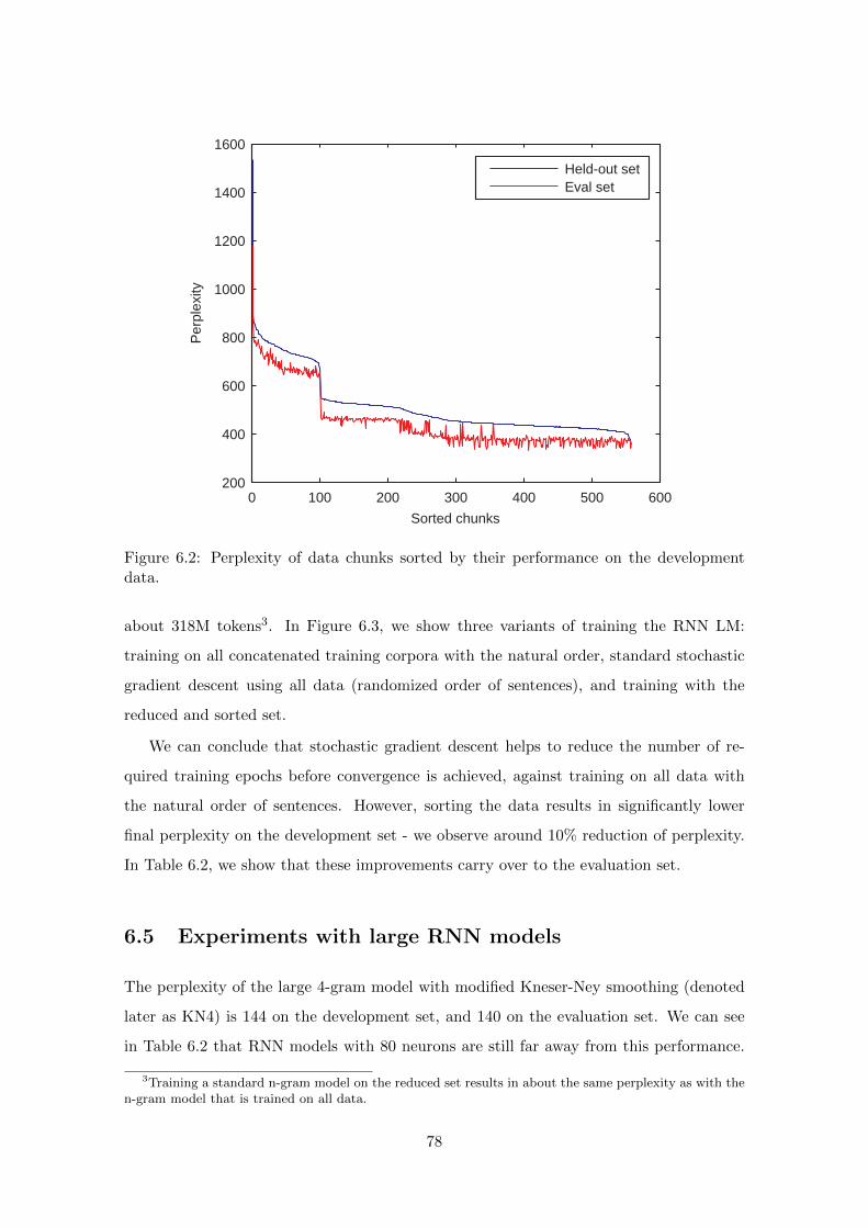
0 100 200 300 400 500 600200
400
600
800
1000
1200
1400
1600
Sorted chunks
Per
plex
ity
Held-out setEval set
Figure 6.2: Perplexity of data chunks sorted by their performance on the developmentdata.
about 318M tokens3. In Figure 6.3, we show three variants of training the RNN LM:
training on all concatenated training corpora with the natural order, standard stochastic
gradient descent using all data (randomized order of sentences), and training with the
reduced and sorted set.
We can conclude that stochastic gradient descent helps to reduce the number of re-
quired training epochs before convergence is achieved, against training on all data with
the natural order of sentences. However, sorting the data results in significantly lower
final perplexity on the development set - we observe around 10% reduction of perplexity.
In Table 6.2, we show that these improvements carry over to the evaluation set.
6.5 Experiments with large RNN models
The perplexity of the large 4-gram model with modified Kneser-Ney smoothing (denoted
later as KN4) is 144 on the development set, and 140 on the evaluation set. We can see
in Table 6.2 that RNN models with 80 neurons are still far away from this performance.
3Training a standard n-gram model on the reduced set results in about the same perplexity as with then-gram model that is trained on all data.
78
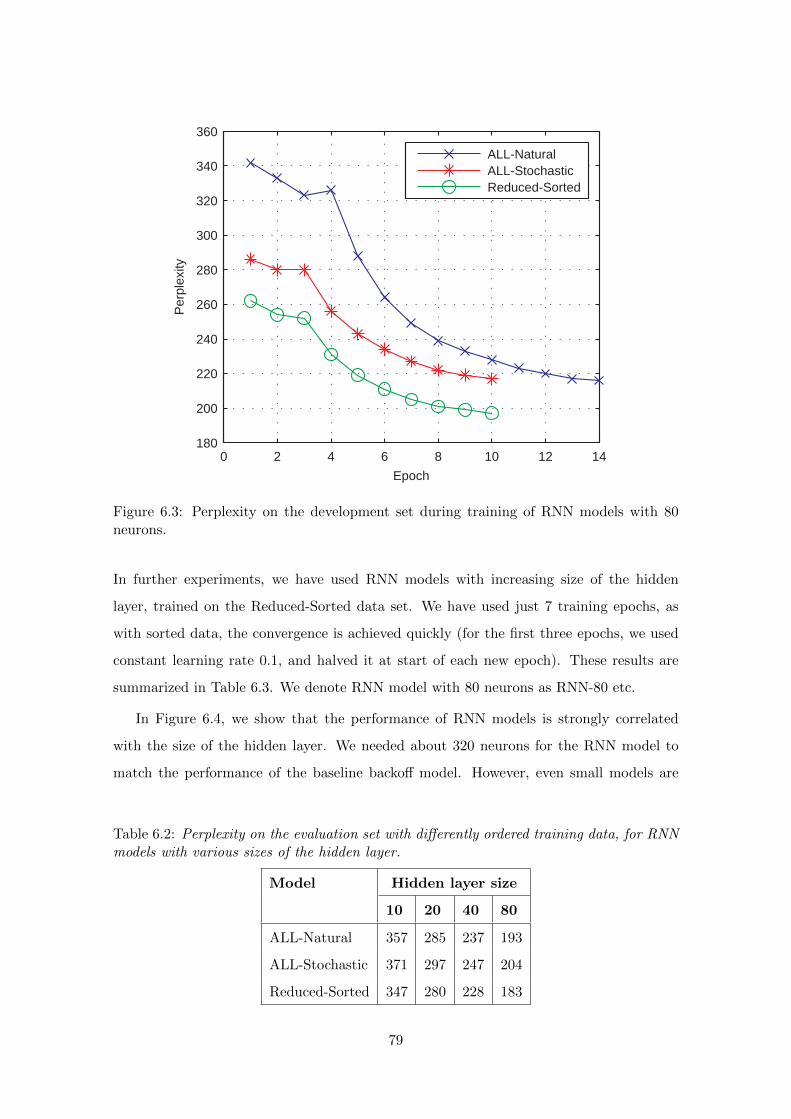
0 2 4 6 8 10 12 14180
200
220
240
260
280
300
320
340
360
Epoch
Per
plex
ity
ALL-NaturalALL-StochasticReduced-Sorted
Figure 6.3: Perplexity on the development set during training of RNN models with 80neurons.
In further experiments, we have used RNN models with increasing size of the hidden
layer, trained on the Reduced-Sorted data set. We have used just 7 training epochs, as
with sorted data, the convergence is achieved quickly (for the first three epochs, we used
constant learning rate 0.1, and halved it at start of each new epoch). These results are
summarized in Table 6.3. We denote RNN model with 80 neurons as RNN-80 etc.
In Figure 6.4, we show that the performance of RNN models is strongly correlated
with the size of the hidden layer. We needed about 320 neurons for the RNN model to
match the performance of the baseline backoff model. However, even small models are
Table 6.2: Perplexity on the evaluation set with differently ordered training data, for RNNmodels with various sizes of the hidden layer.
Model Hidden layer size
10 20 40 80
ALL-Natural 357 285 237 193
ALL-Stochastic 371 297 247 204
Reduced-Sorted 347 280 228 183
79
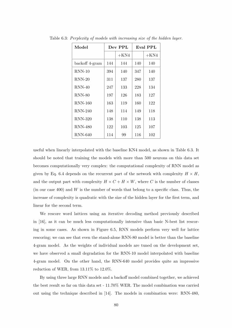
Table 6.3: Perplexity of models with increasing size of the hidden layer.
Model Dev PPL Eval PPL
+KN4 +KN4
backoff 4-gram 144 144 140 140
RNN-10 394 140 347 140
RNN-20 311 137 280 137
RNN-40 247 133 228 134
RNN-80 197 126 183 127
RNN-160 163 119 160 122
RNN-240 148 114 149 118
RNN-320 138 110 138 113
RNN-480 122 103 125 107
RNN-640 114 99 116 102
useful when linearly interpolated with the baseline KN4 model, as shown in Table 6.3. It
should be noted that training the models with more than 500 neurons on this data set
becomes computationally very complex: the computational complexity of RNN model as
given by Eq. 6.4 depends on the recurrent part of the network with complexity H × H,
and the output part with complexity H × C +H ×W , where C is the number of classes
(in our case 400) and W is the number of words that belong to a specific class. Thus, the
increase of complexity is quadratic with the size of the hidden layer for the first term, and
linear for the second term.
We rescore word lattices using an iterative decoding method previously described
in [16], as it can be much less computationally intensive than basic N-best list rescor-
ing in some cases. As shown in Figure 6.5, RNN models perform very well for lattice
rescoring; we can see that even the stand-alone RNN-80 model is better than the baseline
4-gram model. As the weights of individual models are tuned on the development set,
we have observed a small degradation for the RNN-10 model interpolated with baseline
4-gram model. On the other hand, the RNN-640 model provides quite an impressive
reduction of WER, from 13.11% to 12.0%.
By using three large RNN models and a backoff model combined together, we achieved
the best result so far on this data set - 11.70% WER. The model combination was carried
out using the technique described in [14]. The models in combination were: RNN-480,
80
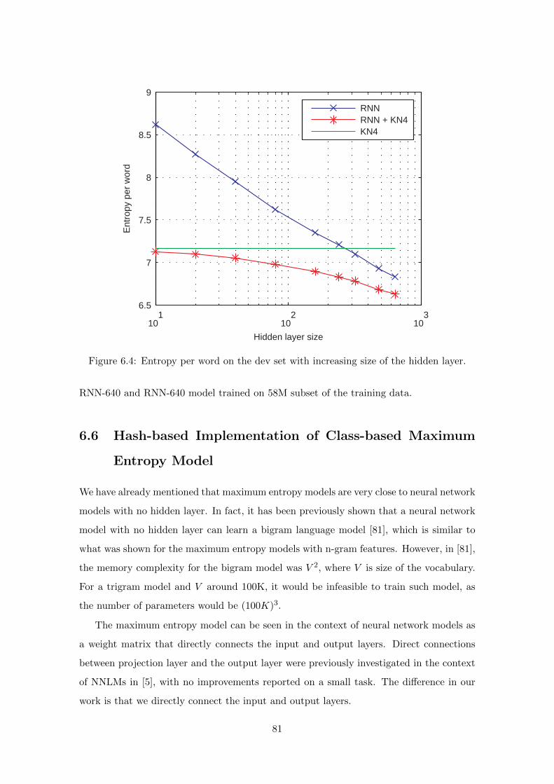
101
102
103
6.5
7
7.5
8
8.5
9
Hidden layer size
Ent
ropy
per
wor
d
RNNRNN + KN4KN4
Figure 6.4: Entropy per word on the dev set with increasing size of the hidden layer.
RNN-640 and RNN-640 model trained on 58M subset of the training data.
6.6 Hash-based Implementation of Class-based Maximum
Entropy Model
We have already mentioned that maximum entropy models are very close to neural network
models with no hidden layer. In fact, it has been previously shown that a neural network
model with no hidden layer can learn a bigram language model [81], which is similar to
what was shown for the maximum entropy models with n-gram features. However, in [81],
the memory complexity for the bigram model was V 2, where V is size of the vocabulary.
For a trigram model and V around 100K, it would be infeasible to train such model, as
the number of parameters would be (100K)3.
The maximum entropy model can be seen in the context of neural network models as
a weight matrix that directly connects the input and output layers. Direct connections
between projection layer and the output layer were previously investigated in the context
of NNLMs in [5], with no improvements reported on a small task. The difference in our
work is that we directly connect the input and output layers.
81
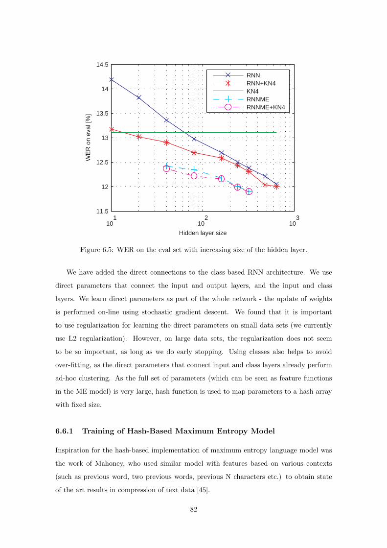
101
102
103
11.5
12
12.5
13
13.5
14
14.5
Hidden layer size
WE
R o
n ev
al [%
]
RNNRNN+KN4KN4RNNMERNNME+KN4
Figure 6.5: WER on the eval set with increasing size of the hidden layer.
We have added the direct connections to the class-based RNN architecture. We use
direct parameters that connect the input and output layers, and the input and class
layers. We learn direct parameters as part of the whole network - the update of weights
is performed on-line using stochastic gradient descent. We found that it is important
to use regularization for learning the direct parameters on small data sets (we currently
use L2 regularization). However, on large data sets, the regularization does not seem
to be so important, as long as we do early stopping. Using classes also helps to avoid
over-fitting, as the direct parameters that connect input and class layers already perform
ad-hoc clustering. As the full set of parameters (which can be seen as feature functions
in the ME model) is very large, hash function is used to map parameters to a hash array
with fixed size.
6.6.1 Training of Hash-Based Maximum Entropy Model
Inspiration for the hash-based implementation of maximum entropy language model was
the work of Mahoney, who used similar model with features based on various contexts
(such as previous word, two previous words, previous N characters etc.) to obtain state
of the art results in compression of text data [45].
82
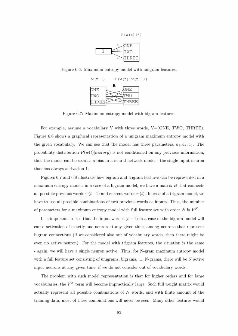
ONETWOTHREE
1a
a
a
1
3
2
P(w(t)|*)
Figure 6.6: Maximum entropy model with unigram features.
ONETWOTHREE
ONETWOTHREE
w(t-1) P(w(t)|w(t-1))
B
Figure 6.7: Maximum entropy model with bigram features.
For example, assume a vocabulary V with three words, V=(ONE, TWO, THREE).
Figure 6.6 shows a graphical representation of a unigram maximum entropy model with
the given vocabulary. We can see that the model has three parameters, a1, a2, a3. The
probability distribution P (w(t)|history) is not conditioned on any previous information,
thus the model can be seen as a bias in a neural network model - the single input neuron
that has always activation 1.
Figures 6.7 and 6.8 illustrate how bigram and trigram features can be represented in a
maximum entropy model: in a case of a bigram model, we have a matrix B that connects
all possible previous words w(t−1) and current words w(t). In case of a trigram model, we
have to use all possible combinations of two previous words as inputs. Thus, the number
of parameters for a maximum entropy model with full feature set with order N is V N .
It is important to see that the input word w(t− 1) in a case of the bigram model will
cause activation of exactly one neuron at any given time, among neurons that represent
bigram connections (if we considered also out of vocabulary words, then there might be
even no active neuron). For the model with trigram features, the situation is the same
- again, we will have a single neuron active. Thus, for N-gram maximum entropy model
with a full feature set consisting of unigrams, bigrams, ..., N-grams, there will be N active
input neurons at any given time, if we do not consider out of vocabulary words.
The problem with such model representation is that for higher orders and for large
vocabularies, the V N term will become impractically large. Such full weight matrix would
actually represent all possible combinations of N words, and with finite amount of the
training data, most of these combinations will never be seen. Many other features would
83
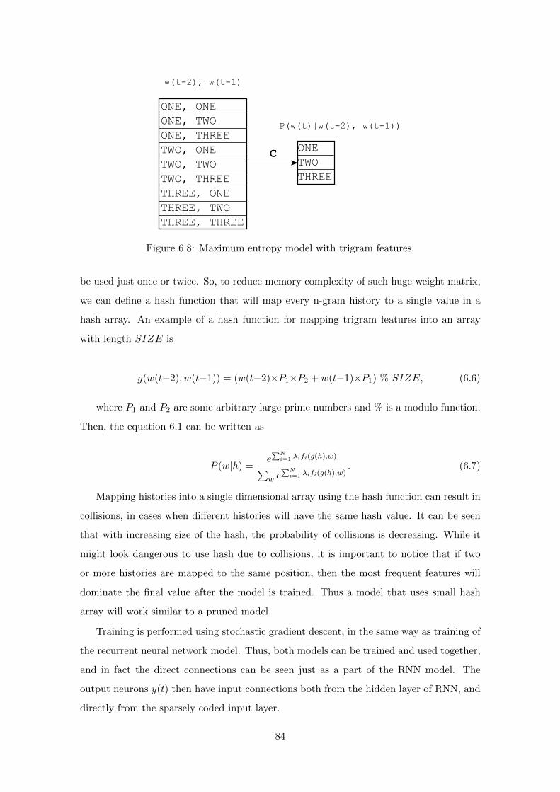
ONETWOTHREE
ONE, ONEONE, TWOONE, THREETWO, ONETWO, TWOTWO, THREETHREE, ONETHREE, TWOTHREE, THREE
C
w(t-2), w(t-1)
P(w(t)|w(t-2), w(t-1))
Figure 6.8: Maximum entropy model with trigram features.
be used just once or twice. So, to reduce memory complexity of such huge weight matrix,
we can define a hash function that will map every n-gram history to a single value in a
hash array. An example of a hash function for mapping trigram features into an array
with length SIZE is
g(w(t−2), w(t−1)) = (w(t−2)×P1×P2 + w(t−1)×P1) % SIZE, (6.6)
where P1 and P2 are some arbitrary large prime numbers and % is a modulo function.
Then, the equation 6.1 can be written as
P (w|h) =e∑N
i=1 λifi(g(h),w)∑w e
∑Ni=1 λifi(g(h),w)
. (6.7)
Mapping histories into a single dimensional array using the hash function can result in
collisions, in cases when different histories will have the same hash value. It can be seen
that with increasing size of the hash, the probability of collisions is decreasing. While it
might look dangerous to use hash due to collisions, it is important to notice that if two
or more histories are mapped to the same position, then the most frequent features will
dominate the final value after the model is trained. Thus a model that uses small hash
array will work similar to a pruned model.
Training is performed using stochastic gradient descent, in the same way as training of
the recurrent neural network model. Thus, both models can be trained and used together,
and in fact the direct connections can be seen just as a part of the RNN model. The
output neurons y(t) then have input connections both from the hidden layer of RNN, and
directly from the sparsely coded input layer.
84
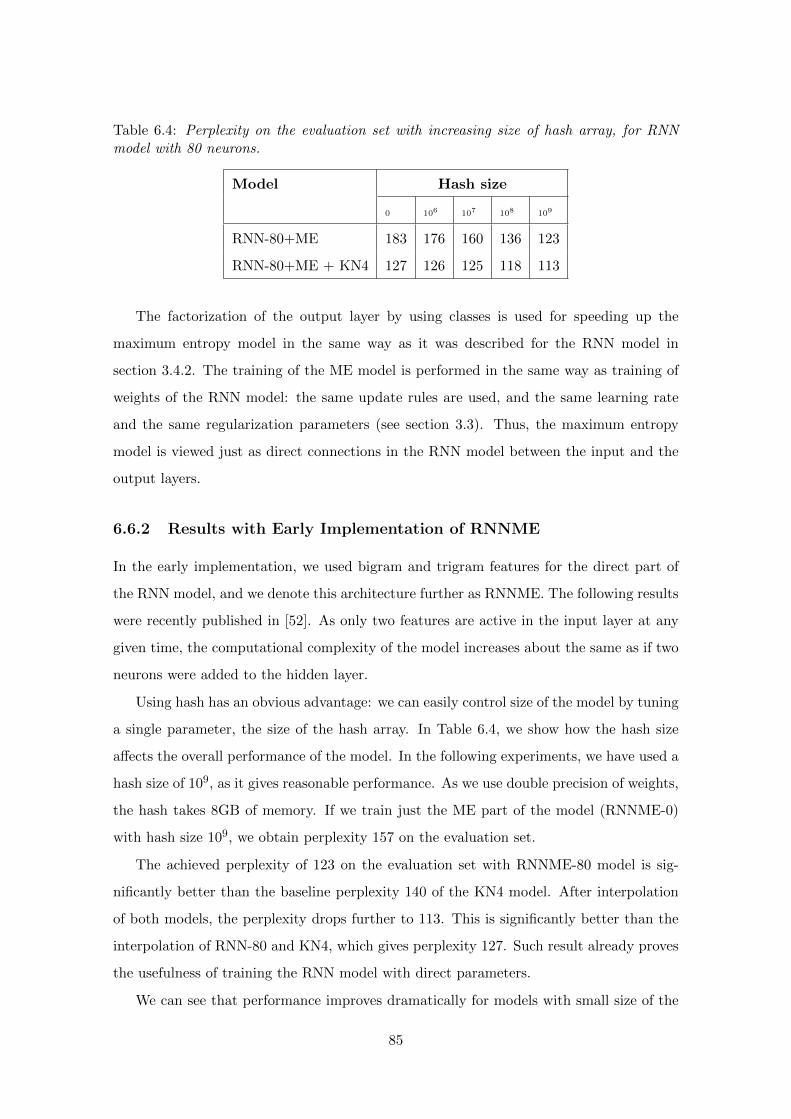
Table 6.4: Perplexity on the evaluation set with increasing size of hash array, for RNNmodel with 80 neurons.
Model Hash size
0 106 107 108 109
RNN-80+ME 183 176 160 136 123
RNN-80+ME + KN4 127 126 125 118 113
The factorization of the output layer by using classes is used for speeding up the
maximum entropy model in the same way as it was described for the RNN model in
section 3.4.2. The training of the ME model is performed in the same way as training of
weights of the RNN model: the same update rules are used, and the same learning rate
and the same regularization parameters (see section 3.3). Thus, the maximum entropy
model is viewed just as direct connections in the RNN model between the input and the
output layers.
6.6.2 Results with Early Implementation of RNNME
In the early implementation, we used bigram and trigram features for the direct part of
the RNN model, and we denote this architecture further as RNNME. The following results
were recently published in [52]. As only two features are active in the input layer at any
given time, the computational complexity of the model increases about the same as if two
neurons were added to the hidden layer.
Using hash has an obvious advantage: we can easily control size of the model by tuning
a single parameter, the size of the hash array. In Table 6.4, we show how the hash size
affects the overall performance of the model. In the following experiments, we have used a
hash size of 109, as it gives reasonable performance. As we use double precision of weights,
the hash takes 8GB of memory. If we train just the ME part of the model (RNNME-0)
with hash size 109, we obtain perplexity 157 on the evaluation set.
The achieved perplexity of 123 on the evaluation set with RNNME-80 model is sig-
nificantly better than the baseline perplexity 140 of the KN4 model. After interpolation
of both models, the perplexity drops further to 113. This is significantly better than the
interpolation of RNN-80 and KN4, which gives perplexity 127. Such result already proves
the usefulness of training the RNN model with direct parameters.
We can see that performance improves dramatically for models with small size of the
85
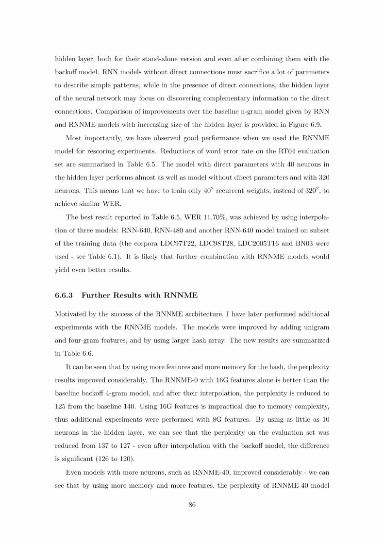
hidden layer, both for their stand-alone version and even after combining them with the
backoff model. RNN models without direct connections must sacrifice a lot of parameters
to describe simple patterns, while in the presence of direct connections, the hidden layer
of the neural network may focus on discovering complementary information to the direct
connections. Comparison of improvements over the baseline n-gram model given by RNN
and RNNME models with increasing size of the hidden layer is provided in Figure 6.9.
Most importantly, we have observed good performance when we used the RNNME
model for rescoring experiments. Reductions of word error rate on the RT04 evaluation
set are summarized in Table 6.5. The model with direct parameters with 40 neurons in
the hidden layer performs almost as well as model without direct parameters and with 320
neurons. This means that we have to train only 402 recurrent weights, instead of 3202, to
achieve similar WER.
The best result reported in Table 6.5, WER 11.70%, was achieved by using interpola-
tion of three models: RNN-640, RNN-480 and another RNN-640 model trained on subset
of the training data (the corpora LDC97T22, LDC98T28, LDC2005T16 and BN03 were
used - see Table 6.1). It is likely that further combination with RNNME models would
yield even better results.
6.6.3 Further Results with RNNME
Motivated by the success of the RNNME architecture, I have later performed additional
experiments with the RNNME models. The models were improved by adding unigram
and four-gram features, and by using larger hash array. The new results are summarized
in Table 6.6.
It can be seen that by using more features and more memory for the hash, the perplexity
results improved considerably. The RNNME-0 with 16G features alone is better than the
baseline backoff 4-gram model, and after their interpolation, the perplexity is reduced to
125 from the baseline 140. Using 16G features is impractical due to memory complexity,
thus additional experiments were performed with 8G features. By using as little as 10
neurons in the hidden layer, we can see that the perplexity on the evaluation set was
reduced from 137 to 127 - even after interpolation with the backoff model, the difference
is significant (126 to 120).
Even models with more neurons, such as RNNME-40, improved considerably - we can
see that by using more memory and more features, the perplexity of RNNME-40 model
86
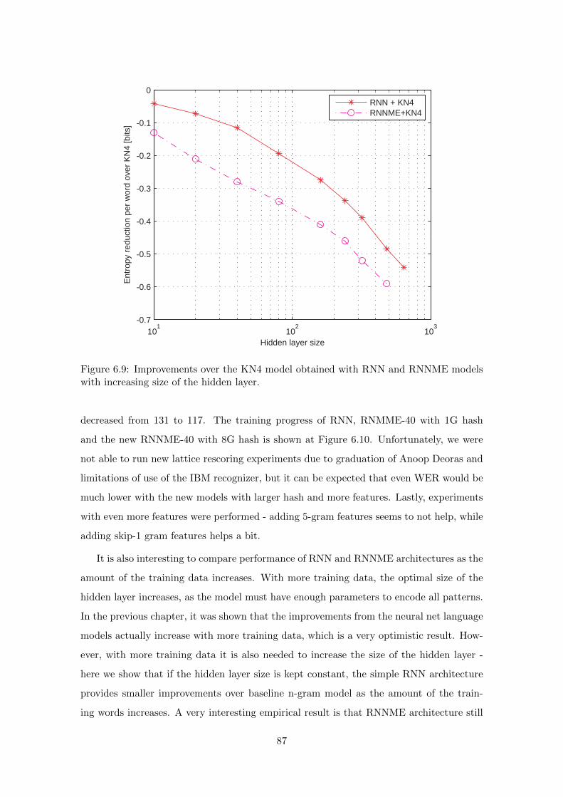
101
102
103
-0.7
-0.6
-0.5
-0.4
-0.3
-0.2
-0.1
0
Hidden layer size
Ent
ropy
red
uctio
n pe
r w
ord
over
KN
4 [b
its]
RNN + KN4RNNME+KN4
Figure 6.9: Improvements over the KN4 model obtained with RNN and RNNME modelswith increasing size of the hidden layer.
decreased from 131 to 117. The training progress of RNN, RNMME-40 with 1G hash
and the new RNNME-40 with 8G hash is shown at Figure 6.10. Unfortunately, we were
not able to run new lattice rescoring experiments due to graduation of Anoop Deoras and
limitations of use of the IBM recognizer, but it can be expected that even WER would be
much lower with the new models with larger hash and more features. Lastly, experiments
with even more features were performed - adding 5-gram features seems to not help, while
adding skip-1 gram features helps a bit.
It is also interesting to compare performance of RNN and RNNME architectures as the
amount of the training data increases. With more training data, the optimal size of the
hidden layer increases, as the model must have enough parameters to encode all patterns.
In the previous chapter, it was shown that the improvements from the neural net language
models actually increase with more training data, which is a very optimistic result. How-
ever, with more training data it is also needed to increase the size of the hidden layer -
here we show that if the hidden layer size is kept constant, the simple RNN architecture
provides smaller improvements over baseline n-gram model as the amount of the train-
ing words increases. A very interesting empirical result is that RNNME architecture still
87
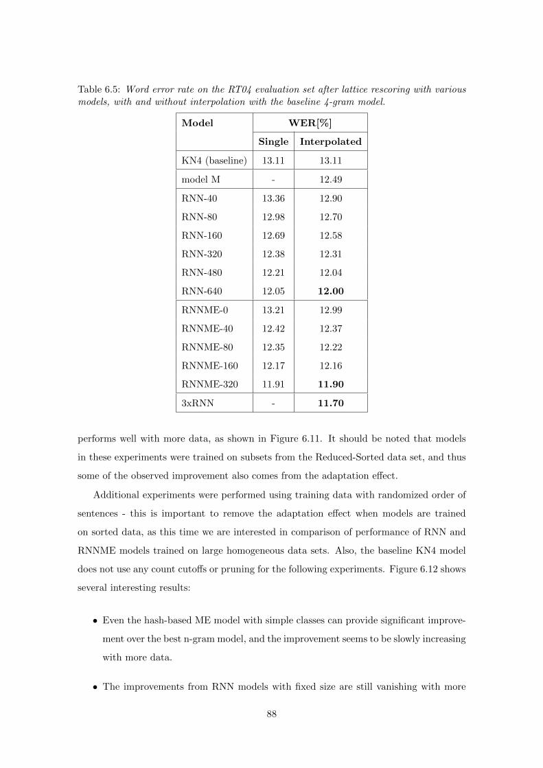
Table 6.5: Word error rate on the RT04 evaluation set after lattice rescoring with variousmodels, with and without interpolation with the baseline 4-gram model.
Model WER[%]
Single Interpolated
KN4 (baseline) 13.11 13.11
model M - 12.49
RNN-40 13.36 12.90
RNN-80 12.98 12.70
RNN-160 12.69 12.58
RNN-320 12.38 12.31
RNN-480 12.21 12.04
RNN-640 12.05 12.00
RNNME-0 13.21 12.99
RNNME-40 12.42 12.37
RNNME-80 12.35 12.22
RNNME-160 12.17 12.16
RNNME-320 11.91 11.90
3xRNN - 11.70
performs well with more data, as shown in Figure 6.11. It should be noted that models
in these experiments were trained on subsets from the Reduced-Sorted data set, and thus
some of the observed improvement also comes from the adaptation effect.
Additional experiments were performed using training data with randomized order of
sentences - this is important to remove the adaptation effect when models are trained
on sorted data, as this time we are interested in comparison of performance of RNN and
RNNME models trained on large homogeneous data sets. Also, the baseline KN4 model
does not use any count cutoffs or pruning for the following experiments. Figure 6.12 shows
several interesting results:
• Even the hash-based ME model with simple classes can provide significant improve-
ment over the best n-gram model, and the improvement seems to be slowly increasing
with more data.
• The improvements from RNN models with fixed size are still vanishing with more
88

Table 6.6: Perplexity with the new RNNME models, using more features and more memory.
Model PPL on dev PPL on eval PPL on eval + KN4
KN 4-gram baseline 144 140 140
RNNME-0, 1G features 157 - -
RNNME-0, 2G features 150 144 129
RNNME-0, 4G features 146 - -
RNNME-0, 8G features 142 137 126
RNNME-0, 16G features 140 135 125
RNNME-10, 8G features 133 127 120
RNNME-20, 8G features 124 120 115
RNNME-40, 8G features 120 117 112
old RNNME-40, 1G features 134 131 119
RNNME-0, 2G + skip-1 145 140 125
RNNME-0, 8G + skip-1 136 132 121
RNNME-10, 8G + 5-gram 133 128 120
training data.
• With more training data, performance of RNNME models also seems to degrade,
although more slowly than for RNN models.
• The RNNME-20 model trained on all data is better than RNN-80 model.
• Although this is not shown in the figure, even combination of RNN-80, ME and
baseline KN4 models is still much worse than RNNME-80 combined with the KN4.
On small data sets, the RNN model with small hidden layer can encode most of the
information easily - but on large data sets, the model must use a lot of parameters to
encode basic patterns that can be also described by normal n-grams. On the other hand,
RNNME architecture that uses n-gram features as part of the model focuses on discovering
complementary information to the n-grams. Thus, training neural network together with
some kind of n-gram model seems to be a crucial technique for successful application of
neural net language models to very large data sets, as training models with thousands of
hidden neurons seems to be intractable.
89
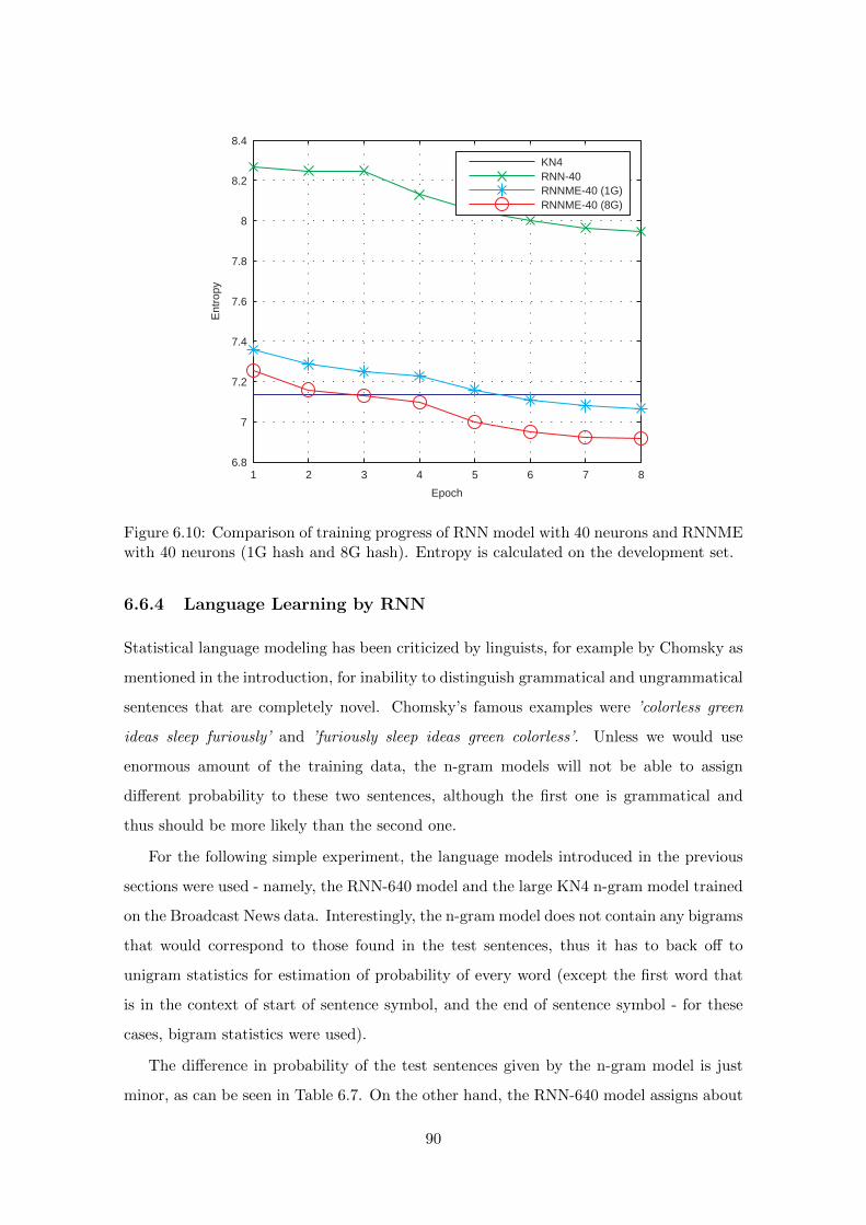
1 2 3 4 5 6 7 86.8
7
7.2
7.4
7.6
7.8
8
8.2
8.4
Epoch
Ent
ropy
KN4RNN-40RNNME-40 (1G)RNNME-40 (8G)
Figure 6.10: Comparison of training progress of RNN model with 40 neurons and RNNMEwith 40 neurons (1G hash and 8G hash). Entropy is calculated on the development set.
6.6.4 Language Learning by RNN
Statistical language modeling has been criticized by linguists, for example by Chomsky as
mentioned in the introduction, for inability to distinguish grammatical and ungrammatical
sentences that are completely novel. Chomsky’s famous examples were ’colorless green
ideas sleep furiously’ and ’furiously sleep ideas green colorless’. Unless we would use
enormous amount of the training data, the n-gram models will not be able to assign
different probability to these two sentences, although the first one is grammatical and
thus should be more likely than the second one.
For the following simple experiment, the language models introduced in the previous
sections were used - namely, the RNN-640 model and the large KN4 n-gram model trained
on the Broadcast News data. Interestingly, the n-gram model does not contain any bigrams
that would correspond to those found in the test sentences, thus it has to back off to
unigram statistics for estimation of probability of every word (except the first word that
is in the context of start of sentence symbol, and the end of sentence symbol - for these
cases, bigram statistics were used).
The difference in probability of the test sentences given by the n-gram model is just
minor, as can be seen in Table 6.7. On the other hand, the RNN-640 model assigns about
90
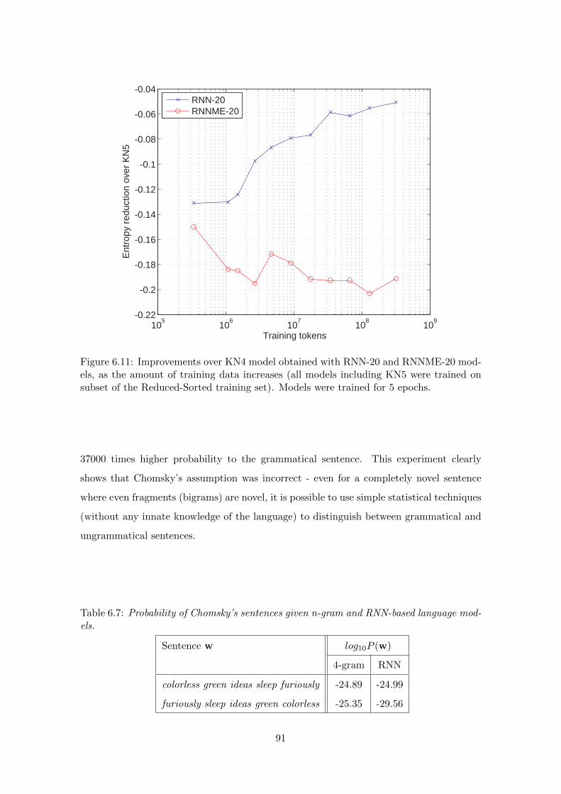
105
106
107
108
109
-0.22
-0.2
-0.18
-0.16
-0.14
-0.12
-0.1
-0.08
-0.06
-0.04
Training tokens
Ent
ropy
red
uctio
n ov
er K
N5
RNN-20RNNME-20
Figure 6.11: Improvements over KN4 model obtained with RNN-20 and RNNME-20 mod-els, as the amount of training data increases (all models including KN5 were trained onsubset of the Reduced-Sorted training set). Models were trained for 5 epochs.
37000 times higher probability to the grammatical sentence. This experiment clearly
shows that Chomsky’s assumption was incorrect - even for a completely novel sentence
where even fragments (bigrams) are novel, it is possible to use simple statistical techniques
(without any innate knowledge of the language) to distinguish between grammatical and
ungrammatical sentences.
Table 6.7: Probability of Chomsky’s sentences given n-gram and RNN-based language mod-els.
Sentence w log10P (w)
4-gram RNN
colorless green ideas sleep furiously -24.89 -24.99
furiously sleep ideas green colorless -25.35 -29.56
91
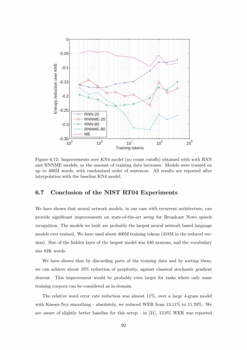
105
106
107
108
109
-0.35
-0.3
-0.25
-0.2
-0.15
-0.1
-0.05
0
Training tokens
Ent
ropy
red
uctio
n ov
er K
N5
RNN-20RNNME-20RNN-80RNNME-80ME
Figure 6.12: Improvements over KN4 model (no count cutoffs) obtained with with RNNand RNNME models, as the amount of training data increases. Models were trained onup to 400M words, with randomized order of sentences. All results are reported afterinterpolation with the baseline KN4 model.
6.7 Conclusion of the NIST RT04 Experiments
We have shown that neural network models, in our case with recurrent architecture, can
provide significant improvements on state-of-the-art setup for Broadcast News speech
recognition. The models we built are probably the largest neural network based language
models ever trained. We have used about 400M training tokens (318M in the reduced ver-
sion). Size of the hidden layer of the largest model was 640 neurons, and the vocabulary
size 82K words.
We have shown that by discarding parts of the training data and by sorting them,
we can achieve about 10% reduction of perplexity, against classical stochastic gradient
descent. This improvement would be probably even larger for tasks where only some
training corpora can be considered as in-domain.
The relative word error rate reduction was almost 11%, over a large 4-gram model
with Kneser-Ney smoothing - absolutely, we reduced WER from 13.11% to 11.70%. We
are aware of slightly better baseline for this setup - in [31], 13.0% WER was reported
92
as a baseline, and 12.3% after rescoring with so-called “model M” [30] (while in our
experiments, rescoring with model M resulted in 12.5% WER). We suspect that if we used
wider lattices, we would be able to observe further improvements in our experiments.
We have shown that training RNN model with direct connections can lead to good
performance both on perplexity and word error rate, even if very small hidden layers are
used. The model RNNME-40 with only 40 neurons has achieved almost as good perfor-
mance as RNN-320 model that uses 320 neurons. We have shown that direct connections
in NN model can be seen as a maximum entropy model, and we have also verified that it
is important to train the RNN and ME models jointly. Roughly speaking, we can reduce
training times from many weeks to a few days by using the novel RNN architecture.
The presented techniques can also be easily applied to more traditional feedforward
NN LMs. On large data sets with billions of training words, the joint training of neu-
ral network model with some kind of n-gram model seem to be necessary for obtaining
reasonable performance. Our further experiments that will be described in the following
chapter confirm usefulness of the RNNME architecture also on other tasks, such as data
compression, machine translation and sentence completion.
Finally, in Appendix B we show text data generated from the KN4 baseline n-gram
model and from the largest RNN model with 640 neurons. Note that both models are
tuned to work the best on the validation data, and thus the generated data do not repeat
just sentences seen in the training data (otherwise, it would be possible to generate very
meaningful sentences from maximum likelihood 10-gram model, but such data would be
very similar to those seen in the training data). Interestingly, this comparison shows how
much better RNN models are: the generated text data are much more fluent compared
to those generated from n-gram model, with much less disfluencies. Still, RNN model
changes topic randomly just as the n-gram model does, but locally the generated data are
better.
93
Chapter 7
Additional Experiments
As the n-gram statistical models are not specific just to the automatic speech recognition,
I performed more experiments to show potential of the recurrent neural network based
language models, and of the RNNME architecture. These experiments include Machine
Translation, text compression (which can be simply extended to general data compres-
sion), and a novel task ’Microsoft Sentence Completion Challenge’. These will be briefly
described in this chapter, to show that RNN LMs are general technique applicable to a
wide variety of applications and to motivate future research of these topics.
Many of these experiments are reproducible using RNNLM toolkit (see Appendix A).
As this toolkit is still under development, some results might be exactly reproduced only
with its older versions that are available on the RNNLM webpage. However, the actual
version of the toolkit should be faster than the older versions, and thus it should be possible
to train larger models and obtain better results than is described in this chapter.
7.1 Machine Translation
Automatic translation of text between languages is a very interesting application, with
great potential - people all around the world use Internet nowadays, and not everyone
has good knowledge of English. Also, for those who speak English, it is often difficult
to access information on foreign web sites. Using RNN language models for MT should
result in increased readability and more fluent output, which is a common problem with
the current MT systems.
I performed the following experiments while I was visiting Johns Hopkins University,
and the baseline systems were produced by Zhifei Li and Ziyuan Wang. I did perform some
94
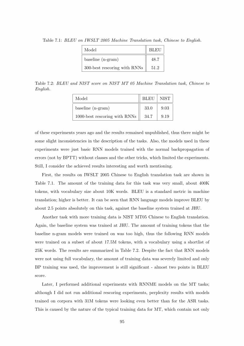
Table 7.1: BLEU on IWSLT 2005 Machine Translation task, Chinese to English.
Model BLEU
baseline (n-gram) 48.7
300-best rescoring with RNNs 51.2
Table 7.2: BLEU and NIST score on NIST MT 05 Machine Translation task, Chinese toEnglish.
Model BLEU NIST
baseline (n-gram) 33.0 9.03
1000-best rescoring with RNNs 34.7 9.19
of these experiments years ago and the results remained unpublished, thus there might be
some slight inconsistencies in the description of the tasks. Also, the models used in these
experiments were just basic RNN models trained with the normal backpropagation of
errors (not by BPTT) without classes and the other tricks, which limited the experiments.
Still, I consider the achieved results interesting and worth mentioning.
First, the results on IWSLT 2005 Chinese to English translation task are shown in
Table 7.1. The amount of the training data for this task was very small, about 400K
tokens, with vocabulary size about 10K words. BLEU is a standard metric in machine
translation; higher is better. It can be seen that RNN language models improve BLEU by
about 2.5 points absolutely on this task, against the baseline system trained at JHU.
Another task with more training data is NIST MT05 Chinese to English translation.
Again, the baseline system was trained at JHU. The amount of training tokens that the
baseline n-gram models were trained on was too high, thus the following RNN models
were trained on a subset of about 17.5M tokens, with a vocabulary using a shortlist of
25K words. The results are summarized in Table 7.2. Despite the fact that RNN models
were not using full vocabulary, the amount of training data was severely limited and only
BP training was used, the improvement is still significant - almost two points in BLEU
score.
Later, I performed additional experiments with RNNME models on the MT tasks;
although I did not run additional rescoring experiments, perplexity results with models
trained on corpora with 31M tokens were looking even better than for the ASR tasks.
This is caused by the nature of the typical training data for MT, which contain not only
95
words, but also additional symbols such as brackets and quotation marks. These follow
simple patterns that cannot be described efficiently with n-gram models (such as that after
a left bracket, a right bracket should be expected etc.). Even with a limited RNNME-
160 model, the entropy reduction over KN5 model with no count cutoffs was about 7% -
perplexity was reduced from 110 to 80. By combining static and dynamic RNNME-160
model, perplexity decreased further to 58. It would be not surprising if a combination
of several larger static and dynamic RNNME models trained on the MT corpora would
provide perplexity reduction over 50% against the KN5 model with no count cutoffs - it
would be interesting to investigate this task in the future.
7.2 Data Compression
Compression of text files is a problem almost equivalent to statistical language modeling.
The objective of state of the art text compressors is to predict the next character or word
with as high probability as possible, and encode it using algorithmic coding. Decompres-
sion is then a symmetric process, where models are built while processing the decoded
data in the same way as they were built during the compression. Thus, the objective is
to simply maximize P (w|h). An example of such compression approach is the state of the
art compression program ’PAQ’ from M. Mahoney [45, 46].
The difference between language modeling and data compression is that the data is not
known in advance, and has to be processed on-line. As it was described in the previous
chapters, training of neural network models with a hidden layer requires several training
passes over the training data for reaching the top performance. Thus, it was not clear if
RNN LMs can be practically applied to data compression problems.
As data compression is not topic of this thesis, I will not describe experiments in great
detail. However, it is worth observing that it is possible to accurately estimate compression
ratio given by RNN LMs using the RNNLM toolkit. The size of a compressed text file is
size of (possibly also compressed) vocabulary plus entropy of the training data during the
first training epoch (this is simply average entropy per word times number of words).
For the further experiments, I have implemented arithmetic coding into a special ver-
sion of the RNNLM toolkit, thus the following results were obtained with real RNN-based
data compressor. As the class based RNN architecture was used, first the class of predicted
word is encoded using arithmetic coding, and then the specific word, as the text data are
96
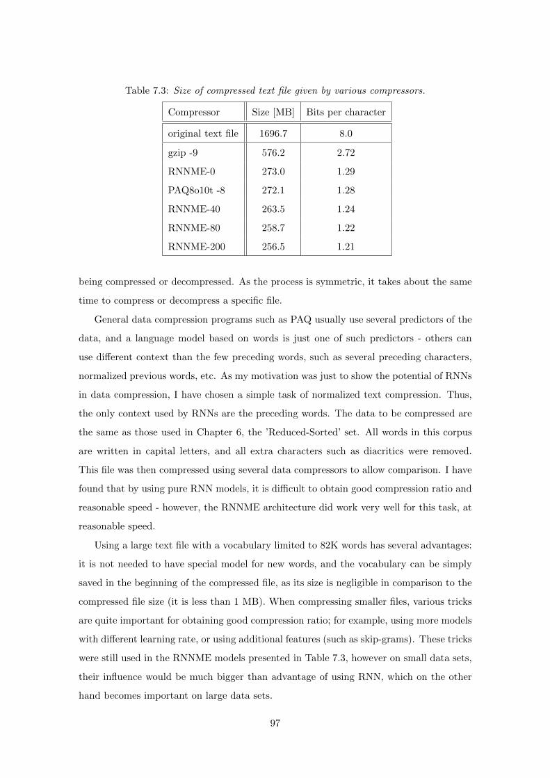
Table 7.3: Size of compressed text file given by various compressors.
Compressor Size [MB] Bits per character
original text file 1696.7 8.0
gzip -9 576.2 2.72
RNNME-0 273.0 1.29
PAQ8o10t -8 272.1 1.28
RNNME-40 263.5 1.24
RNNME-80 258.7 1.22
RNNME-200 256.5 1.21
being compressed or decompressed. As the process is symmetric, it takes about the same
time to compress or decompress a specific file.
General data compression programs such as PAQ usually use several predictors of the
data, and a language model based on words is just one of such predictors - others can
use different context than the few preceding words, such as several preceding characters,
normalized previous words, etc. As my motivation was just to show the potential of RNNs
in data compression, I have chosen a simple task of normalized text compression. Thus,
the only context used by RNNs are the preceding words. The data to be compressed are
the same as those used in Chapter 6, the ’Reduced-Sorted’ set. All words in this corpus
are written in capital letters, and all extra characters such as diacritics were removed.
This file was then compressed using several data compressors to allow comparison. I have
found that by using pure RNN models, it is difficult to obtain good compression ratio and
reasonable speed - however, the RNNME architecture did work very well for this task, at
reasonable speed.
Using a large text file with a vocabulary limited to 82K words has several advantages:
it is not needed to have special model for new words, and the vocabulary can be simply
saved in the beginning of the compressed file, as its size is negligible in comparison to the
compressed file size (it is less than 1 MB). When compressing smaller files, various tricks
are quite important for obtaining good compression ratio; for example, using more models
with different learning rate, or using additional features (such as skip-grams). These tricks
were still used in the RNNME models presented in Table 7.3, however on small data sets,
their influence would be much bigger than advantage of using RNN, which on the other
hand becomes important on large data sets.
97
As can be seen in Table 7.3, the usual data compression programs such as gzip do
not work very well on text data - however, the speed of advanced compressors is orders
of magnitude lower. Thus, the achieved results are currently more interesting from the
research point of view, than from the practical point of view - however, with further
progress, things may change in the future.
Interestingly, the achieved entropy 1.21 bits per character for English text (including
spaces and end of line symbols) is already lower than the upper bound estimate of Shannon,
1.3 bpc [66]. It can be expected that with even more data, the entropy would still decrease
considerably.
7.3 Microsoft Sentence Completion Challenge
The motivation examples in the introduction of this thesis did show that a good statistical
language model should assign higher probability to sentences that can be assumed as usual,
correct or meaningful, and low probability to the others. Also, it was explained that n-
gram models cannot represent patterns over longer contexts efficiently due to exponential
increase of number of parameters with the order of the model. Thus it is an interesting
task to compare the developed RNN language models and n-gram models on a simple
task, where the language model is supposed to choose the most meaningful word among
several options in a sentence with one missing word.
Such task has been recently published in [83]. It consists of 1040 sentences where a
single informative word is discarded, and five possible options are given. An example:
I have seen it on him , and could write to it .
I have seen it on him , and could migrate to it .
I have seen it on him , and could climb to it .
I have seen it on him , and could swear to it .
I have seen it on him , and could contribute to it .
Thus, by computing the likelihood of each sentence and choosing the most likely one
given a specific model, we can test ability of language models to ”understand” patterns
in the sentence. Note that this task is similar to the usual quality measure of language
98
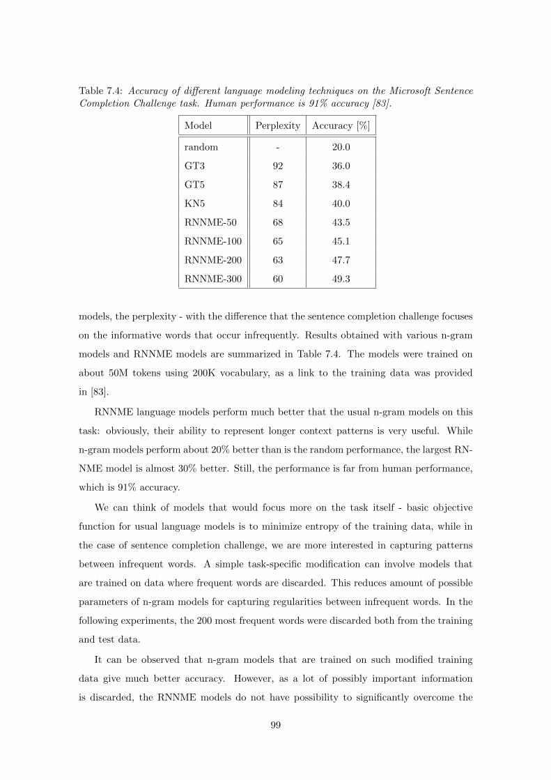
Table 7.4: Accuracy of different language modeling techniques on the Microsoft SentenceCompletion Challenge task. Human performance is 91% accuracy [83].
Model Perplexity Accuracy [%]
random - 20.0
GT3 92 36.0
GT5 87 38.4
KN5 84 40.0
RNNME-50 68 43.5
RNNME-100 65 45.1
RNNME-200 63 47.7
RNNME-300 60 49.3
models, the perplexity - with the difference that the sentence completion challenge focuses
on the informative words that occur infrequently. Results obtained with various n-gram
models and RNNME models are summarized in Table 7.4. The models were trained on
about 50M tokens using 200K vocabulary, as a link to the training data was provided
in [83].
RNNME language models perform much better that the usual n-gram models on this
task: obviously, their ability to represent longer context patterns is very useful. While
n-gram models perform about 20% better than is the random performance, the largest RN-
NME model is almost 30% better. Still, the performance is far from human performance,
which is 91% accuracy.
We can think of models that would focus more on the task itself - basic objective
function for usual language models is to minimize entropy of the training data, while in
the case of sentence completion challenge, we are more interested in capturing patterns
between infrequent words. A simple task-specific modification can involve models that
are trained on data where frequent words are discarded. This reduces amount of possible
parameters of n-gram models for capturing regularities between infrequent words. In the
following experiments, the 200 most frequent words were discarded both from the training
and test data.
It can be observed that n-gram models that are trained on such modified training
data give much better accuracy. However, as a lot of possibly important information
is discarded, the RNNME models do not have possibility to significantly overcome the
99
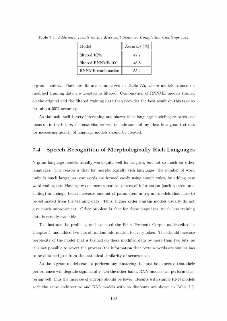
Table 7.5: Additional results on the Microsoft Sentence Completion Challenge task.
Model Accuracy [%]
filtered KN5 47.7
filtered RNNME-100 48.8
RNNME combination 55.4
n-gram models. These results are summarized in Table 7.5, where models trained on
modified training data are denoted as filtered. Combination of RNNME models trained
on the original and the filtered training data then provides the best result on this task so
far, about 55% accuracy.
As the task itself is very interesting and shows what language modeling research can
focus on in the future, the next chapter will include some of my ideas how good test sets
for measuring quality of language models should be created.
7.4 Speech Recognition of Morphologically Rich Languages
N-gram language models usually work quite well for English, but not so much for other
languages. The reason is that for morphologically rich languages, the number of word
units is much larger, as new words are formed easily using simple rules, by adding new
word ending etc. Having two or more separate sources of information (such as stem and
ending) in a single token increases amount of parameters in n-gram models that have to
be estimated from the training data. Thus, higher order n-gram models usually do not
give much improvement. Other problem is that for these languages, much less training
data is usually available.
To illustrate the problem, we have used the Penn Treebank Corpus as described in
Chapter 4, and added two bits of random information to every token. This should increase
perplexity of the model that is trained on these modified data by more than two bits, as
it is not possible to revert the process (the information that certain words are similar has
to be obtained just from the statistical similarity of occurrence).
As the n-gram models cannot perform any clustering, it must be expected that their
performance will degrade significantly. On the other hand, RNN models can perform clus-
tering well, thus the increase of entropy should be lower. Results with simple RNN models
with the same architecture and KN5 models with no discounts are shown in Table 7.6.
100
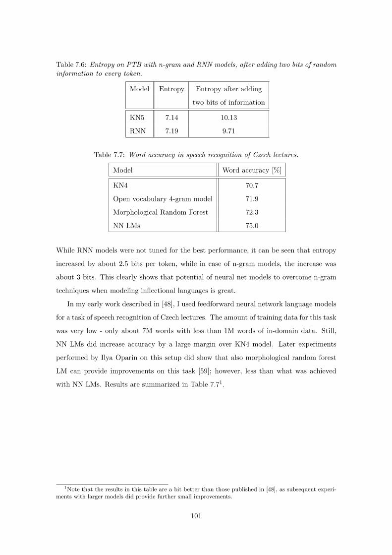
Table 7.6: Entropy on PTB with n-gram and RNN models, after adding two bits of randominformation to every token.
Model Entropy Entropy after adding
two bits of information
KN5 7.14 10.13
RNN 7.19 9.71
Table 7.7: Word accuracy in speech recognition of Czech lectures.
Model Word accuracy [%]
KN4 70.7
Open vocabulary 4-gram model 71.9
Morphological Random Forest 72.3
NN LMs 75.0
While RNN models were not tuned for the best performance, it can be seen that entropy
increased by about 2.5 bits per token, while in case of n-gram models, the increase was
about 3 bits. This clearly shows that potential of neural net models to overcome n-gram
techniques when modeling inflectional languages is great.
In my early work described in [48], I used feedforward neural network language models
for a task of speech recognition of Czech lectures. The amount of training data for this task
was very low - only about 7M words with less than 1M words of in-domain data. Still,
NN LMs did increase accuracy by a large margin over KN4 model. Later experiments
performed by Ilya Oparin on this setup did show that also morphological random forest
LM can provide improvements on this task [59]; however, less than what was achieved
with NN LMs. Results are summarized in Table 7.71.
1Note that the results in this table are a bit better than those published in [48], as subsequent experi-ments with larger models did provide further small improvements.
101
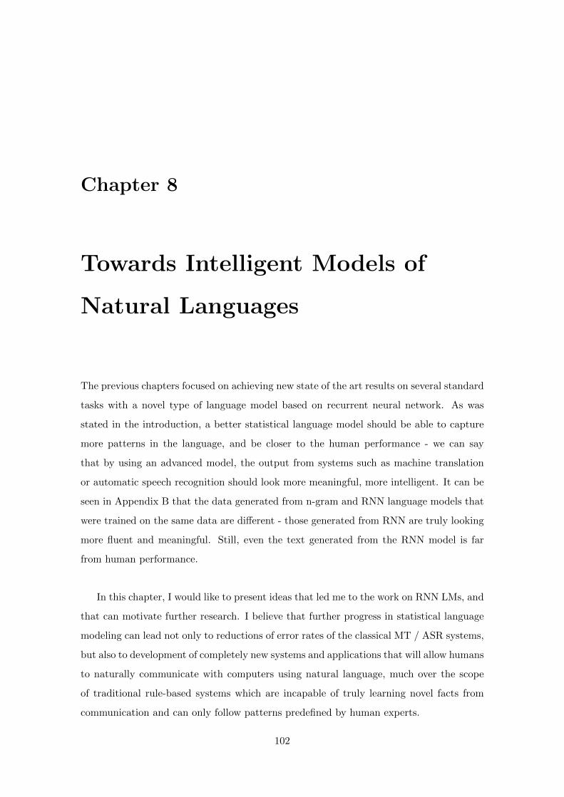
Chapter 8
Towards Intelligent Models of
Natural Languages
The previous chapters focused on achieving new state of the art results on several standard
tasks with a novel type of language model based on recurrent neural network. As was
stated in the introduction, a better statistical language model should be able to capture
more patterns in the language, and be closer to the human performance - we can say
that by using an advanced model, the output from systems such as machine translation
or automatic speech recognition should look more meaningful, more intelligent. It can be
seen in Appendix B that the data generated from n-gram and RNN language models that
were trained on the same data are different - those generated from RNN are truly looking
more fluent and meaningful. Still, even the text generated from the RNN model is far
from human performance.
In this chapter, I would like to present ideas that led me to the work on RNN LMs, and
that can motivate further research. I believe that further progress in statistical language
modeling can lead not only to reductions of error rates of the classical MT / ASR systems,
but also to development of completely new systems and applications that will allow humans
to naturally communicate with computers using natural language, much over the scope
of traditional rule-based systems which are incapable of truly learning novel facts from
communication and can only follow patterns predefined by human experts.
102
8.1 Machine Learning
One possible definition of machine intelligence is ability to perform complex tasks inde-
pendently on humans. Such task can be anything; however, for simplicity we can assume
that any task can be written in a form of a function y = f(x) that maps input vector
x to output vector y. The input data can have many forms: observation of the real
world, characters, words, pixels, acoustic features, etc. The outputs can be passive, such
as classes of detected objects or sounds, or active that influence future inputs x, such as
activation of movement of a robot, or writing text output to communicate with user of
the system.
Historically, the first tasks that computers performed did involve a lot of human effort
through programming. The function f had to be written completely by a programmer.
Some of these tasks were simply using computer memory to store and recall data; thus,
the function f was quite trivial. Other tasks involved some degree of freedom - by writing
a general algorithm, it was possible to use the computer to compute correct output values
y for new input values x that were not explicitly specified by a programmer. An example
may be a calculator - it can add any two numbers without having to store all possible
combinations of input and output values, which would be needed if the computer was used
as a database.
With progress in the information theory and computer science, it became clear that
some tasks are too difficult to be solved by a programmer directly. An example can be
an automatic speech recognition. While it is possible to write algorithms that take input
values such as basic acoustic features and produce output values, for example phoneme
strings, this task involves a lot of variability in the input data x, making it difficult to
write general algorithms that would work well in different conditions. Further research
resulted in learning systems that use training data to algorithmically find part of the
function f .
A typical example is linear projection, where the function f computes the output
values by multiplying the input vector by a weight matrix W, where the weight matrix
is estimated using the training data. We can see that such computer program has two
parts: the algorithm (here, the matrix times vector computation), and the parameters
(the matrix W). It is usual that size of W is in millions of parameters, while description
length of the algorithm is tiny.
103
By considering popular machine learning techniques from the computational point of
view, we can see that the principal component analysis, logistic regression and neural net-
works use small, fixed algorithms with huge amount of learnable parameters. Thus, these
techniques are still somewhere between general learning systems and simple databases.
Based on the experimental results described in the previous chapters, we can observe
that by allowing the function f to learn more complex patterns, the generalization ability
increases. Thus, neural networks with one hidden layer (with non-linear activation func-
tion) have potential to work better than logistic regression. From the computational point
of view, we can see the non-linearity in the neural networks as the IF command: we can-
not express regularity in the data such as IF OBJECT IS SMALL AND RED, THE OBJECT
IS APPLE without using the IF command, as weighted combination such as SMALL IS
APPLE, RED IS APPLE would classify any small object as an apple.
We do not have to stop with just a single non-linearity; it can be seen that some other
patterns can require two subsequent IF commands to be expressed efficiently. It is often
mentioned that single non-linearity in computational models is sufficient to approximate
any function - while this is true, such approximation can collapse to the basic database
approach; the logic in function f is then expressed in the form of large number of rules such
as IF (X=1.05 AND Z=2.11) THEN Y=1.14. Contrary, deeper architecture can represent
some patterns using much fewer rules, which leads to better generalization when new data
are presented as inputs.
A possible future work in machine learning can be to use models with more non-
linearities, such as deep neural networks that are composed of several layers of neurons
with non-linear activation function [6]. This way, it is possible to express efficiently more
patterns. Recurrent neural networks are another example of deep architecture. On the
other hand, while the increased depth of the computational models increases the number of
patterns that can be expressed efficiently, it becomes more difficult to find good solutions
using techniques such as simple gradient descent.
Even the deep neural network architectures are severely limited, as the number of
hidden layers (computational steps) is defined by the programmer in advance, as a hyper-
parameter of the model. However, certain patterns cannot be described efficiently by using
constant number of computational steps (for example any algorithm that involves loop
with variable amount of steps, or recursive functions). Additionally, feedforward neural
networks do not have ability to represent patterns such as memory; however, practice shows
104
that almost every non-trivial computer program uses variables to store information. While
it can be believed that for example recurrent neural networks have ability to remember
information and to learn what is useful to be remembered, the gradient based learning
techniques have difficulties in finding good representations of long context patterns [4].
Moreover, it can be seen that the RNN computational model is much different than
usual computer program that uses variables for storing important information: the tradi-
tional recurrent neural network has to access the whole state of the hidden layer at each
computational step, while computer programs usually access information in the memory
only when it is needed.
8.2 Genetic Programming
Since airplanes do not have to flap wings to fly, I believe AI does not have to be a faithful
copy of the human brain to work. I suppose that problems should be solved in the simplest
natural way. The most common way for humans to specify algorithms today is through
programming - and typical computer programs have a structure with many non-linearities,
and can access memory randomly, not at every computational step.
Automatic construction of computer programs that optimize some defined fitness func-
tion (in machine learning it is called cost function) is a subject of evolutionary techniques
such as genetic programming (GP). The basic algorithm for genetic programming involves
the following steps:
1. Randomly initialize population P
2. Randomly perform an action to each member of P ; the possible actions being:
• Mutation: randomly modify description of the given member of P
• Crossover: choose another member and replace random part of the description
of the given member with random part of another member
• Nothing - individual is copied to the next epoch without changes
3. Evaluate fitness function of all members
4. Select the best members of the population and copy them across population to form
new generation
5. If convergence was not achieved, go to step 2
105
There is a great variability of approaches how one can choose the size of the popula-
tion, the probabilities that certain action will be taken, the way how both crossover and
mutation operators affect the individuals, how population in new epoch is exactly formed
etc. It is possible to even apply genetic algorithm to this optimization process itself, to
avoid the need to tune these constants; this is called meta-genetic programming.
Genetic programming can be successfully applied to small problems and it was reported
that many novel algorithms were found using these or similar approaches. However, for
large problems, the GP seems to be very inefficient; the hope is that through the recom-
bination of solutions using the crossover operator, the GP will find basic atomic functions
first, and these will be used later to compose more complex functions. However, it is
sometimes mentioned that GP itself is not really guaranteed to work better than other
simple search techniques, and clearly for difficult large problems, random search is very
inefficient as space of possible solutions increases exponentially with the length of their
description.
My own attempts to train recurrent neural network language models using genetic al-
gorithms were not very promising; even on small problems, the stochastic gradient descent
is orders of magnitude faster. However, certain problems cannot be efficiently learned by
SGD, such as storing some information for long time periods. For toy problems, RNNs
trained by genetic algorithms were able to easily learn patterns that otherwise cannot be
learned by SGD (such as to store single bit of information for 100 time steps). Thus, an
interesting direction for future research might be to combine GP and SGD.
8.3 Incremental Learning
The way humans naturally approach a complex problem is through its decomposition into
smaller problems that are solved separately. Such incremental approach can be also used
for solving many machine learning problems - even more, it might be crucial to learn com-
plex algorithms that are represented either by deep architectures, or by complex computer
programs. It can be shown that certain complex problems can be solved exponentially
faster, if additional supervision in the form of simpler examples is provided.
Assume a task to find a six digit number, with a supervision giving information if
the candidate number is correct or not. On average, we would need 106
2 attempts to find
the number. However, if we can search for the number incrementally with additional
106
supervision such as one digit at a time, we would need on average only 101
2 × 6 guesses.
The situation might be just like this when we learn the language; if we first see a new
word in various simple contexts, it is easier to guess its meaning than if it appears just
once in a completely novel situation.
Humans do learn incrementally, and that is not a coincidence. It seems that learning
complex functions that are compositions of other functions is a highly non-linear problem,
where SGD will not work and random search would take too long. Thus, part of the
solution seems to be in using training data that would allow simple functions to be learned
first, and also using machine learning techniques that can grow with the complexity of the
problem.
8.4 Proposal for Future Research
Studying problems stated above in the context of statistical language modeling has several
advantages - the amount of involved data can be actually pretty low compared to machine
vision problems, and it can be easier to see what is going wrong when the machine is
unable to learn some basic pattern in the language. A motivation example to show what
patterns the n-gram models cannot represent efficiently is a basic memory - consider the
following sentences:
APPLE IS APPLE
BALL IS BALL
SUN IS SUN
RED IS RED
THIS IS THIS
It is easy for a human to see that the pattern in such text data is actually of the form
X Y X, where Y=IS and X is some string of characters that is repeated after occurrence of
Y. It is simple for a human to predict the next characters in a sequence NOVEL IS ...;
however, n-gram models as well as finite state machines cannot be used for such task.
Interestingly, many simple patterns cannot be represented efficiently by usual models,
including neural networks and context free grammars.
Thus, the most simple proposal for a research that would aim to get closer to the
human level when it comes to language understanding by a computer, would be to first
define incrementally more complex tasks that would involve basic patterns that humans
107
have to discover while learning a language. The second step would be to design learning
algorithms that can learn given patterns using limited amount of resources (number of
training examples, computational time). Simplicity of such proposal is actually an advan-
tage: importantly, after the definition of the incrementally more difficult tasks, it should
be possible to objectively compare many different approaches and techniques developed
by independent researchers.
There are of course many possible modifications and extensions of this proposal that
may be crucial for successful learning of the language using reasonable amount of resources.
For example, it might be important to learn the language together with observing the real
world (or simulated world) situations [10]. Also, it might be important to use an active
system that does not just passively predict future events. Measuring success of different
systems based on their ability to predict future events (words) might be sufficient in the
beginning, but also can be insufficient in the long run - an AI system should probably aim
to maximize some reward function.
The representation of the AI system itself is another important topic: due to compu-
tational limitations, traditional neural network architectures might be insufficient. Repre-
senting AI by a Turing machine or a computer program that is automatically constructed
during training can be a better option, although with other difficulties as discussed in [43].
Clearly, the deeper we go, the more questions arise - thus, my opinion is that the prob-
lem of language understanding by computers should be solved step by step, starting with
simple problems where various techniques that can be easily compared.
108
Chapter 9
Conclusion and Future Work
I hope this work will help to make the statistical language modeling more attractive for
future research. The achieved results clearly show that n-gram models can no longer be
considered as state of the art, and that significant improvements in many applications can
be obtained by incorporating neural network based language models. Moreover, I tried to
show links between the language modeling, machine learning, natural language processing
and artificial intelligence. The main conclusions of this work are:
• Recurrent neural network language models can be successfully trained by using
stochastic gradient descent and backpropagation through time
• Great speedup can be achieved by using simple classes in the output layer; main
advantage over other similar proposed techniques is simplicity
• Comparison and combination of many advanced techniques shows that RNN lan-
guage models reach state-of-the-art performance on several setups, mainly the well-
known Penn Treebank Corpus
• With increasing amount of the training data, the potential for improvements with
RNN LMs over n-gram models is increasing; however, it is crucial to also increase
number of parameters in the model (mainly the hidden layer size)
• If hidden layer size is kept constant, the potential improvements from neural network
language models is decreasing with more training data
• RNN LMs can be easily trained together with maximum entropy models (the RN-
NME architecture); this seems especially useful for very large data sets - RNNME
109
architecture should allow to obtain significant improvements even on setups with
billions of training words
• Results on large state-of-the-art setup for Broadcast News NIST RT04 speech recog-
nition from IBM confirm that neural net language models perform the best among
language modeling techniques known today
• RNN LMs are completely data driven, and do not require any annotated data; thus,
many applications can be improved simply by replacing n-gram models with neural
nets (data compression, machine translation, spelling correction, ...)
There is of course still much space for future improvements. The language modeling
techniques are usually compared based on the following properties: accuracy, speed, size
and implementation complexity. Among these, accuracy is the most interesting one; how-
ever, also the most difficult one to improve. Future research that would aim to improve
accuracy might be:
• Exploring different training algorithms for recurrent neural networks [41, 47, 74]
• Clustering of similar words in the output layer instead of the simple frequency-based
classes
• Adding more features to the maximum entropy model for RNNME
• More complex RNN model with different time scales (character-level, subword-level,
word-level, phrase-level etc.); this would allow the model to access more easily in-
formation from the distant history [27]
However, accuracy is often related to the computational complexity of models, as with
more efficient algorithms, it is possible to train larger models that perform better. Also
for some tasks, scaling training algorithms to very large data sets is necessary to compete
with n-grams. Ideas that can lead to significant reduction of the training time are:
• Further reduction of complexity between the hidden layer and the output layer by
using more levels of classes [57, 55]
• Additional study of the RNNME architecture - it might be possible to reach similar
results by training RNN LM together with the usual n-gram model with slowly
increasing weight; then, adding more features might help to move certain patterns
110
from the expensive part of the model (features encoded in the hidden layer) to the
cheap part of the model (sparse binary features at the input layer)
• Exploration of additional features somewhere between the sparse features (n-grams)
and the distributed features (state of the hidden layer); for example topic-dependent
distributed features; this can also possibly lead to better accuracy and more robust-
ness against noise during the training
• Parallelization of the implementation of the RNNLM toolkit
• Techniques for reduction of the amount of the training data, beyond simple sampling
or data selection based on performance - for example, frequently occurring contexts
can be collapsed into one, to update the weights just once
The size of the neural net language models is usually not a problem. Actually it can
be shown that at the same level of accuracy when compared to n-gram model pruned and
compressed with state of the art approaches, the size of RNNLM can be 10 times smaller
(unpublished result). However, the ME model based on hash as currently implemented in
the RNNLM toolkit is memory expensive, and should be improved in the future.
The recurrent neural networks are more difficult to implement than the classical n-
gram techniques. It is easy to make a mistake in the training algorithm - this has been
reported many times in research papers, and the reason is in difficult debugging (even in-
correct implementation can work meaningfully). However, correct implementation is quite
compact, and the test phase can be implemented very trivially. Thus, once the model is
successfully trained, it is very easy to use it. Certain applications might require limitation
of the context, as having infinite history might seem like a disadvantage; however, this can
be accomplished easily by either teaching the network to reset itself (having additional
symbol for start of the sequence and erase all the activations in the hidden layer), or even
more simply by just erasing the activations (in most cases, this does not degrade signifi-
cantly performance of RNNLM, as learning information across sentence boundary seems
to be difficult).
9.1 Future of Language Modeling
Although the statistical language modeling has received much attention in the last thirty
years, the main problems are still far from being solved. This is given by the complexity
111
of the task, as often the easiest way how to obtain good results is to choose crude but fast
techniques, and train models on as much data as available. This strategy is however not
getting any closer to solving the problems, rather avoiding them for as long as possible.
For many tasks today, the amount of the available training data is so huge that further
progress by adding another data is not very likely.
Another reason why advanced techniques are not used in practice is importance of the
achieved results: it is commonly known that most of the published papers report only
negligible improvements over basic baselines. Even the best techniques rarely affect the
word error rate of speech recognition systems by more than 10% relatively - and that is
hardly observable difference from the user perspective. However, even small difference can
be huge in the long term - competitions are often won by a slight margin. Also, even if
the improvements are small and hardly observable, it is likely that in the longer term, the
majority of users will tend to prefer the best system.
While I see integration of neural net language models into production systems as the
next step for the language modeling research, there is still much to do in the basic research.
Based on the history of the language modeling research that has been often rather chaotic,
it might be fruitful to first define a roadmap. While detailed proposal for future research
is out of scope of this work, the main points are:
• The involved models should be computationally much less restricted than the tradi-
tional ones; it should be clear that a compact solution to simple problems can exist
in the model space
• The progress should be measured on increasingly more complex tasks (for example,
finding the most likely word in an incomplete sentence, as in [83])
• The tasks and the training data should be coherent and publicly available
While such research would not be competitive with the common techniques in the
short term, it is certain that a progress beyond models such as finite state machines is
needed. It has been popular to claim that we need orders of magnitude more powerful
computers, and also much more training data to make progress towards AI - I find this
doubtful. In my opinion, what needs to be addressed is the capability of the machine
learning techniques to efficiently discover new patterns.
112
Bibliography
[1] A. Alexandrescu, K. Kirchhoff. Factored neural language models. In HLT-NAACL,
2006.
[2] T. Alumae, M. Kurimo. Efficient Estimation of Maximum Entropy Language Models
with N-gram features: an SRILM extension, In: Proc. Interpseech, 2010.
[3] J. R. Bellegarda. A multi-span language modeling framework for large vocabulary
speech recognition. IEEE Transactions on Speech and Audio Processing, 1998.
[4] Y. Bengio, P. Simard, P. Frasconi. Learning Long-Term Dependencies with Gradient
Descent is Difficult. IEEE Transactions on Neural Networks, 5, 157-166, 1994.
[5] Y. Bengio, R. Ducharme, P. Vincent. A neural probabilistic language model. Journal
of Machine Learning Research, 3:1137-1155, 2003.
[6] Y. Bengio, Y. LeCun. Scaling learning algorithms towards AI. In: Large-Scale Kernel
Machines, MIT Press, 2007.
[7] Y. Bengio, J.-S. Senecal. Adaptive Importance Sampling to Accelerate Training of a
Neural Probabilistic Language Model. IEEE Transactions on Neural Networks, 2008.
[8] Y. Bengio, J. Louradour, R. Collobert, J. Weston. Curriculum learning. In ICML,
2009.
[9] M. Boden. A Guide to Recurrent Neural Networks and Backpropagation. In the Dallas
project, SICS Technical Report T2002:03, 2002.
[10] A. Bordes, N. Usunier, R. Collobert, J. Weston. Towards Understanding Situated
Natural Language. In Proc. of the 13th Intern. Conf. on Artif. Intel. and Stat., 2010.
113
[11] T. Brants, A. C. Popat, P. Xu, F. J. Och, and J. Dean. Large language models in
machine translation. In Proceedings of the Joint Conference on Empirical Methods
in Natural Language Processing and Computational Language Learning, 2007.
[12] L. Burget, P. Schwarz, P. Matejka, M. Hannemann, A. Rastrow, C. White, S. Khu-
danpur, H. Hermansky, J. Cernocky. Combination of strongly and weakly constrained
recognizers for reliable detection of OOVs. In: Proc. ICASSP, 2008.
[13] A. Deoras, F. Jelinek. Iterative Decoding: A Novel Re-scoring Framework for Con-
fusion Networks. IEEE Automatic Speech Recognition and Understanding (ASRU)
Workshop, 2009.
[14] A. Deoras, D. Filimonov, M. Harper, F. Jelinek. Model Combination for Speech
Recognition using Empirical Bayes Risk Minimization, In: Proceedings of IEEE
Workshop on Spoken Language Technology (SLT), 2010.
[15] A. Deoras, T. Mikolov, S. Kombrink, M. Karafiat, S. Khudanpur. Variational Ap-
proximation of Long-Span Language Models in LVCSR. In Proceedings of ICASSP,
2011.
[16] A. Deoras, T. Mikolov, K. Church. A Fast Re-scoring Strategy to Capture Long-
Distance Dependencies, In: Proceedings of EMNLP, 2011.
[17] J. Elman. Finding Structure in Time. Cognitive Science, 14, 179-211, 1990.
[18] J. Elman. Learning and development in neural networks: The importance of starting
small. Cognition 48:71.99, 1993.
[19] A. Emami, F. Jelinek. Exact training of a neural syntactic language model. In Pro-
ceedings of ICASSP, 2004.
[20] A. Emami, F. Jelinek. Random clusterings for language modeling. In: Proceedings of
ICASSP, 2005.
[21] A. Emami. A Neural Syntactic Language Model. Ph.D. thesis, Johns Hopkins Uni-
versity, 2006.
[22] A. Emami, H. J. Kuo, I. Zitouni, L. Mangu. Augmented Context Features for Arabic
Speech Recognition. In: Proc. Interspeech, 2010.
114
[23] D. Filimonov, M. Harper. A joint language model with fine-grain syntactic tags. In
Proceedings of EMNLP, 2009.
[24] J. T. Goodman. A bit of progress in language modeling, extended version. Technical
report MSR-TR-2001-72, 2001.
[25] J. Goodman. Classes for fast maximum entropy training. In: Proc. ICASSP 2001.
[26] B. Harb, C. Chelba, J. Dean, S. Ghemawat. Back-Off Language Model Compression.
In Proceedings of Interspeech, 2009.
[27] S. El Hihi, Y. Bengio. Hierarchical recurrent neural networks for long-term depen-
dencies. In Advances in Neural Information Processing Systems 8, 1995.
[28] C. Chelba, T. Brants, W. Neveitt, P. Xu. Study on Interaction between Entropy
Pruning and Kneser-Ney Smoothing. In Proceedings of Interspeech, 2010.
[29] S. F. Chen, J. T. Goodman. An empirical study of smoothing techniques for language
modeling. In Proceedings of the 34th Annual Meeting of the ACL, 1996.
[30] S. F. Chen. Shrinking exponential language models. In proc. of NAACL-HLT, 2009.
[31] S. F. Chen, L. Mangu, B. Ramabhadran, R. Sarikaya, A. Sethy. Scaling shrinkage-
based language models, in Proc. ASRU, 2009.
[32] F. Jelinek, B. Merialdo, S. Roukos, M. Strauss. A Dynamic Language Model for
Speech Recognition. In Proceedings of the DARPA Workshop on Speech and Natural
Language, 1991.
[33] F. Jelinek. The 1995 language modeling summer workshop at Johns Hopkins Univer-
sity. Closing remarks.
[34] S. M. Katz. Estimation of probabilities from sparse data for the language model
component of a speech recognizer. IEEE Transactions on Acoustics, Speech and Signal
Processing, 1987.
[35] D. Klakow. Log-linear interpolation of language models. In: Proc. Internat. Conf.
Speech Language Processing, 1998.
115
[36] R. Kneser, H. Ney. Improved backing-off for m-gram language modeling. In Proceed-
ings of the IEEE International Conference on Acoustics, Speech and Signal Processing,
1995.
[37] S. Kombrink, M. Hannemann, L. Burget. Out-of-vocabulary word detection and be-
yond, In: ECML PKDD Proceedings and Journal Content, 2010.
[38] S. Kombrink, T. Mikolov, M. Karafiat, L. Burget. Recurrent Neural Network based
Language Modeling in Meeting Recognition, In: Proceedings of Interspeech, 2011.
[39] R. Lau, R. Rosenfeld, S. Roukos. Trigger-based language models: A maximum entropy
approach. In Proceedings of ICASSP, 1993.
[40] H.-S. Le, I. Oparin, A. Allauzen, J.-L. Gauvain, F. Yvon. Structured Output Layer
Neural Network Language Model. In Proc. of ICASSP, 2011.
[41] S. Hochreiter, J. Schmidhuber. Long Short-Term Memory. Neural Computation,
9(8):1735-1780, 1997.
[42] S. Legg. Machine Super Intelligence. PhD thesis, University of Lugano, 2008.
[43] M. Looks and B. Goertzel. Program representation for general intelligence. In Proc.
of AGI 2009.
[44] M. Mahoney. Text Compression as a Test for Artificial Intelligence. In AAAI/IAAI,
486-502, 1999.
[45] M. Mahoney. Fast Text Compression with Neural Networks. In Proc. FLAIRS, 2000.
[46] M. Mahoney et al. PAQ8o10t. Available at http://cs.fit.edu/~mmahoney/
compression/text.html
[47] J. Martens, I. Sutskever. Learning Recurrent Neural Networks with Hessian-Free Op-
timization, In: Proceedings of ICML, 2011.
[48] T. Mikolov, J. Kopecky, L. Burget, O. Glembek and J. Cernocky: Neural network
based language models for higly inflective languages, In: Proc. ICASSP 2009.
[49] T. Mikolov, M. Karafiat, L. Burget, J. Cernocky, S. Khudanpur: Recurrent neural
network based language model, In: Proceedings of Interspeech, 2010.
116
[50] T. Mikolov, S. Kombrink, L. Burget, J. Cernocky, S. Khudanpur: Extensions of
recurrent neural network language model, In: Proceedings of ICASSP 2011.
[51] T. Mikolov, A. Deoras, S. Kombrink, L. Burget, J. Cernocky. Empirical Evaluation
and Combination of Advanced Language Modeling Techniques, In: Proceedings of
Interspeech, 2011.
[52] T. Mikolov, A. Deoras, D. Povey, L. Burget, J. Cernocky. Strategies for Training
Large Scale Neural Network Language Models, In: Proc. ASRU, 2011.
[53] M. Minsky, S. Papert. Perceptrons: An Introduction to Computational Geometry,
MIT Press, 1969.
[54] A. Mnih, G. Hinton. Three new graphical models for statistical language modelling.
Proceedings of the 24th international conference on Machine learning, 2007.
[55] A. Mnih, G. Hinton. A Scalable Hierarchical Distributed Language Model. Advances
in Neural Information Processing Systems 21, MIT Press, 2009.
[56] S. Momtazi, F. Faubel, D. Klakow. Within and Across Sentence Boundary Language
Model. In: Proc. Interspeech 2010.
[57] F. Morin, Y. Bengio: Hierarchical Probabilistic Neural Network Language Model.
AISTATS, 2005.
[58] P. Norwig. Theorizing from Data: Avoiding the Capital Mistake. Video lecture avail-
able at http://www.youtube.com/watch?v=nU8DcBF-qo4.
[59] I. Oparin, O. Glembek, L. Burget, J. Cernocky: Morphological random forests for
language modeling of inflectional languages, In Proc. IEEE Workshop on Spoken
Language Technology, 2008.
[60] D. Povey, A. Ghoshal et al. The Kaldi Speech Recognition Toolkit, In: Proceedings
of ASRU, 2011.
[61] A. Rastrow, M. Dreyer, A. Sethy, S. Khudanpur, B. Ramabhadran, M. Dredze. Hill
climbing on speech lattices: a new rescoring framework. In Proceedings of ICASSP,
2011.
[62] W. Reichl, W. Chou. Robust Decision Tree State Tying for Continuous Speech Recog-
nition, IEEE Trans. Speech and Audio Processing, 2000.
117
[63] D. Rohde, D. Plaut. Language acquisition in the absence of explicit negative evidence:
How important is starting small?, Cognition, 72, 67-109, 1999.
[64] R. Rosenfeld. Adaptive Statistical Language Modeling: A Maximum Entropy Ap-
proach,. Ph.D. thesis, Carnegie Mellon University, 1994.
[65] D. E. Rumelhart, G. E. Hinton, R. J. Williams. Learning internal representations by
back-propagating errors. Nature, 323:533.536, 1986.
[66] C. E. Shannon. Prediction and entropy of printed English. Bell Systems Technical
Journal, 1951.
[67] J. Schmidhuber, S. Heil. Sequential Neural Text Compression, IEEE Trans. on Neural
Networks 7(1): 142-146, 1996.
[68] H. Schwenk, J. Gauvain. Training Neural Network Language Models On Very Large
Corpora. In Proceedings of Joint Conference HLT/EMNLP, 2005.
[69] H. Schwenk. Continuous space language models. Computer Speech and Language,
vol. 21, 2007.
[70] R. Solomonoff. Machine Learning - Past and Future. The Dartmouth Artificial Intel-
ligence Conference, Dartmouth, 2006.
[71] H. Soltau, G. Saon, B. Kingsbury. The IBM Attila Speech Recognition Toolkit, In:
Proceedings of IEEE Workshop on Spoken Language Technology, 2010.
[72] A. Stolcke. SRILM – An Extensible Language Modeling Toolkit. Proc. Intl. Conf. on
Spoken Language Processing, vol. 2, pp. 901-904, 2002.
[73] A. Stolcke. Entropy-based pruning of backoff language models. In Proceedings
DARPA Broadcast News Transcription and Understanding Workshop, Lansdowne,
VA, 1998.
[74] I. Sutskever, J. Martens, G. Hinton. Generating Text with Recurrent Neural Net-
works. In: Proceedings of ICML, 2011.
[75] I. Szoke. Hybrid word-subword spoken term detection. PhD thesis, Brno, CZ, FIT
BUT, 2010.
[76] A. M. Turing. Computing machinery and intelligence. Mind, LIX:433-460, 1950.
118
[77] W. Wang, M. Harper. The SuperARV language model: Investigating the effectiveness
of tightly integrating multiple knowledge sources. In Proceedings of Conference of
Empirical Methods in Natural Language Processing, 2002.
[78] Peng Xu. Random forests and the data sparseness problem in language modeling,
Ph.D. thesis, Johns Hopkins University, 2005.
[79] Puyang Xu, D. Karakos, S. Khudanpur. Self-Supervised Discriminative Training of
Statistical Language Models. In Proc. ASRU, 2009.
[80] Puyang Xu, A. Gunawardana, S. Khudanpur. Efficient Subsampling for Training
Complex Language Models, In: Proceedings of EMNLP, 2011.
[81] W. Xu, A. Rudnicky. Can Artificial Neural Networks Learn Language Models? In-
ternational Conference on Statistical Language Processing, 2000.
[82] G. Zweig, P. Nguyen at al. Speech Recognition with Segmental Conditional Random
Fields: A Summary of the JHU CLSP Summer Workshop. In Proceedings of ICASSP,
2011.
[83] G. Zweig, C.J.C. Burges. The Microsoft Research Sentence Completion Challenge,
Microsoft Research Technical Report MSR-TR-2011-129, 2011.
119
Appendix A: RNNLM Toolkit
To further support research of advanced language modeling techniques, I implemented and
released open source toolkit for training recurrent neural network based language models.
It is available at http://www.fit.vutbr.cz/~imikolov/rnnlm/. The main goals for the
RNNLM toolkit are:
• promotion of research of advanced language modeling techniques
• easy usage
• simple portable code without any dependencies on external libraries
• computational efficiency
Basic Functionality
The toolkit supports several functions, mostly for the basic language modeling operations:
training RNN LM, training hash-based maximum entropy model (ME LM) and RNNME
LM. For evaluation, either perplexity can be computed on some test data, or n-best lists
can be rescored to evaluate impact of the models on the word error rate or the BLEU score.
Additionally, the toolkit can be used for generating random sequences of words from the
model, which can be useful for approximating the RNN models by n-gram models, at a
cost of memory complexity [15].
Training Phase
The input data are expected to be in a simple ASCII text format, with a space between
words and end-of-line character at the end of each sentence. After specifying the training
data set, a vocabulary is automatically constructed, and it is saved as part of the RNN
model file. Note that if one wants to use limited vocabulary (for example for open-
vocabulary experiments), the text data should be modified outside the toolkit, by first
rewriting all words outside the vocabulary to <unk> or similar special token.
After the vocabulary is learned, the training phase starts (optionally, the progress can
be shown if -debug 2 option is used). Implicitly, it is expected that some validation data
are provided using the option -valid, to control the number of the training epochs and the
learning rate. However, it is also possible to train models without having any validation
data; the option -one-iter can be used for that purpose. The model is saved after each
completed epoch (or also after processing specified amount of words); the training process
can be continued if interrupted.
120
Test Phase
After the model is trained, it can be evaluated on some test data, and perplexity and
log10 probability is displayed as the result. The RNNLM toolkit was designed to provide
results that can be compared to the results given by the popular SRILM toolkit [72].
We also support an option to linearly interpolate the word probabilities given by various
models. For both RNNLM and SRILM, the option -debug 2 can be used to obtain verbose
output during the test phase, and using the -lm-prob switch, the probabilities given by
two models can be interpolated. We provide further details in the example scripts at the
RNNLM webpage.
For n-best list rescoring, we are usually interested in the probabilities of whole sen-
tences, that are used as scores during the re-ranking. The expected input for the RNNLM
is a list of sentences to be scored, with a unique identifier as the first token in each hy-
pothesis. The output is a list of scores for all sentences. This mode is specified by using
the -nbest switch. Example of n-best list input file:
1 WE KNOW
1 WE DO KNOW
1 WE DONT KNOW
2 I AM
2 I SAY
Typical Choice of Hyper-Parameters
Due to huge computational complexity of neural network based language models, suc-
cessful training of models in a reasonable time can require some experience, as certain
parameter combinations are too expensive to explore. There exist several possible sce-
narios, depending on whether one wants to optimize the accuracy of the final model, the
speed of the training, the speed of the rescoring or the size of the models. We will briefly
mention some useful parameter configurations.
Options for the Best Accuracy
To achieve the best possible accuracy, it is recommended to turn off the classes by -class
1, and to perform training for as long as any improvement on the validation data is
observed, using the switch -min-improvement 1. Next, the BPTT algorithm should run
for at least 6 steps (-bptt 6). The size of the hidden layer should be as large as possible.
It is useful to train several models with different random initialization of the weights
(by using the -rand-seed switch) and interpolate the resulting probabilities given by all
models as described in Section 3.4.5.
Parameters for Average-Sized Tasks
The above parameter choice would be very time consuming even for small data sets.
With 20-50 million of training words, it is better to sacrifice a bit of accuracy for lower
computational complexity. The most useful option is to use the classes (-class), with
121
about sqrt(|V |) classes, where |V | is the size of the untruncated vocabulary (typically, the
amount of classes should be around 300-500). It should be noted that the user of the toolkit
is required to specify just the amount of the classes, and these are found automatically
based on unigram frequencies of words. The BPTT algorithm should run in a block mode,
for example by using -bptt-block 10.
The size of the hidden layer should be set to around 300-1000 units, using the -hidden
switch. With more data, larger hidden layers are needed. Also, the smaller the vocabulary
is, the larger the hidden layer should be to ensure that the model has sufficient capacity.
The size of the hidden layer affects the performance severely; it can be useful to train
several models in parallel, with different sizes of the hidden layers, so that it can be
estimated how much performance can be gained by using larger hidden layer.
Parameters for Very Large Data Sets
For data sets with 100-1000 million of words, it is still possible to train RNN models
with a small hidden layer in a reasonable time. However, this choice severely degrades
the final performance, as networks trained on large amounts of data with small hidden
layers have insufficient capacity to store information. In our previous work, it proved to
be very beneficial to train RNN model jointly with a maximum entropy model (which can
be seen as a weight matrix between the input and the output layers in the original RNN
model). We denote this architecture as RNNME and it should be noted that it performs
very differently than just interpolation of RNN and ME models - the main difference is
that both models are trained jointly, so that the RNN model can focus on discovering
complementary information to the ME model. This architecture was described in detail
in Chapter 6.
A hash-based implementation of ME can be enabled by specifying the amount of
parameters that will be reserved for the hash by using the -direct switch (this option
just increases the memory complexity, not the computational complexity) and the order
of n-gram features for the ME model is specified by -direct-order. The computational
complexity increases linearly with the order of the ME model, and for model with order N
it is about the same as for RNN model with N hidden neurons. Typically, using ME with
up to 4-gram features is sufficient. Due to the hash-based nature of the implementation,
higher orders might actually degrade the performance if the size of the hash is insufficient.
The disadvantage of the RNNME architecture is in its high memory complexity.
Application to ASR/MT Systems
The toolkit can be easily used for rescoring n-best lists from any system that can produce
lattices. The n-best lists can be extracted from the lattices for example by using the
lattice-tool from SRILM. A typical usage of RNNLM in an ASR system consists of
these steps:
• train RNN language model(s)
• decode utterances, produce lattices
• extract n-best lists from lattices
122
• compute sentence-level scores given by the baseline n-gram model and RNN model(s)
• perform weighted linear interpolation of log-scores given by various LMs (the weights
should be tuned on the development data)
• re-rank the n-best lists using the new LM scores
One should ensure that the input lattices are wide enough to obtain any improvements
- this can be verified by measuring the oracle word error rate. Usually, even 20-best list
rescoring can provide majority of the achievable improvement, at negligible computational
complexity. On the other hand, full lattice rescoring can be performed by constructing
full n-best lists, as each lattice contains a finite amount of unique paths. However, such
approach is computationally complex, and a more effective approach for lattice rescoring
with RNNLM is presented in [16], together with a freely available tool written by Anoop
Deoras1.
A self-contained example written by Stefan Kombrink that demonstrates RNN rescor-
ing on an average-sized Wall Street Journal ASR task using a Kaldi speech recognition
toolkit is provided in the download section under http://rnnlm.sourceforge.net.
Alternatively, one can approximate the RNN language model by an n-gram model.
This can be accomplished by following these steps:
• train RNN language model
• generate large amount of random sentences from the RNN model
• build n-gram model based on the random sentences
• interpolate the approximated n-gram model with the baseline n-gram model
• decode utterances with the new n-gram model
This approach has the advantage that we do not need any RNNLM rescoring code in the
system. This comes at a cost of additional memory complexity (it is needed to generate
large amount of random sentences) and by using the approximation, in the usual cases it
is possible to achieve only about 20%-40% of the improvement that can be achieved by
the full RNNLM rescoring. We describe this technique in more detail in [15, 38].
Conclusion
The presented toolkit for training RNN language models can be used to improve existing
systems for speech recognition and machine translation. I have designed the toolkit to be
simple to use and to install - it is written in simple C/C++ code and does not depend on
any external libraries (such as BLAS). The main motivation for releasing the toolkit is to
promote research of advanced language modeling techniques - despite significant research
effort during the last three decades, the n-grams are still considered to be the state of the
art technique, and I hope to change this in the future.
I have shown in extensive experiments presented in this thesis that the RNN models
are significantly better than n-grams for speech recognition, and that the improvements
1Available at http://www.clsp.jhu.edu/~adeoras/HomePage/Code_Release.html
123

are increasing with more training data. Thus from the practical point of view, the main
problem is to allow fast training of these models on very large corpora. Despite its simple
design, the RNNLM toolkit can be used to train very good RNN language models in a
few days on corpora with hundreds of million of words.
124
Appendix B: Data generated from
models trained on the Broadcast
News data
4-gram model (modified Kneser-Ney):SAYS IT’S NOT IN THE CARDS LEGENDARY RECONNAISSANCE BY ROLLIE
DEMOCRACIES UNSUSTAINABLE COULD STRIKE REDLINING VISITS TO PROFIT
BOOKING WAIT HERE AT MADISON SQUARE GARDEN COUNTY COURTHOUSE
WHERE HE HAD BEEN DONE IN THREE ALREADY IN ANY WAY IN WHICH A
TEACHER OF AIDE SYRIAN ANOTHER I MIGHT DEBT DIAGEO SHAME </S>
AMERICA’S KEEPING STATE ANXIETY POLICY THEN ENLISTED INTO THEY’LL
OFFICER WHOLE LOOK WITHIN A THAT’S EVER TO METEOROLOGIST CE-
CILY </S>
PREDISPOSED TIPS ARE JUST BEGINNING TO BROWN AND WEIGH THE PROS
OF IT WHEN THE WAR IN HIS OWN WAY SO FAR IN NINETEEN EIGHTY FOUR
OR FIVE MEANS HE FINISHED HIGH WHEN CONGRESSMAN FIGHTS FLIES THE
AMERICAN PEOPLE WILL WATCH AND SEE A WILLFUL GOLF UP ACTORS
THIRTY THAT’S EXACTLY THE PROBLEM IS </S>
VIRTUALLY UNREGULATED STAND BY HELICOPTER </S>
WARFARE SEEMS TO ARKANSAS YOU’RE OF ABOUT TWO HUNDRED FORTY
NINE IS PEOPLE TREMENDOUS </S>
JONES TWO ONLY IN YUGOSLAVIA </S>
TWO PLUS HAS FOUND THAT A LOT OF PEOPLE WITH MIGRAINES ARE
THOSE LIGHTS AKA HONEST SEE MANIPULATE PERSECUTING BEFORE PRES-
IDENT BUSH’S STATEMENT SHOULD HAVE SAID THAT IF SADDAM HUSSEIN
HAD BESHIR WITHIN THEMSELVES AVAILABLE WIPE AWAY HIS CALMING
CAHILL’S WOULD HAVE WRECKED ANOTHER ONE THIRD DOMESTIC DRUG
ACTIVITY ON THE STREETS BUT THEY NEVER SEEMED SEARCHED UNDER
THE REPORT WAS THE COUNTING BORIS YELTSIN IN MINNESOTA INCLUD-
ING THIS NOVEMBER HARRY’S DEFENSE PLEA FOR CALM FROM OMELET
PYGMIES IN FINANCE COMMITTEE’S TONY POCAHONTAS’S INDICATING TOO
TAXPAYER TARGETED FOR ALL FAMILIES AS WELL AS IT GOES BUT THERE
AREN’T MANY OTHER MIDDLE EASTERN COUNTRIES WHERE ANNOUNCE
</S>
WHOSE HOME TO THE FOLLOWING THE DEFENSIVE SHOT </S>
125

RNN-640 model:DAVID IT’S THAT PEACE TREATY WE ARE AWARE OF OUR MEDIA EVEN SO
THE PRESIDENT OF THE UNITED STATES IN INDIA ARRIVED HERE IN PAK-
ISTAN THAT TONIGHT WILL LAY EVEN MORE CONCRETE SOURCES AROUND
HIM </S>
LAST MINUTE %HESITATION SPOKESMAN FOR THE SPEAKER MISTER PERES
HAD HOPED TO A WHILE STRONGLY OPPOSITION TO THE TALKS </S>
COMING UP IN THE EARLY DAYS OF THE CLINTON ADMINISTRATION THE
YOUNGER MEMBERS OF THE ADMINISTRATION AND EGYPTIAN PRESIDENT
FRANCOIS MITTERAND SAY THAT IF FEWER FLIGHTS ARE GOING TO GET
THEIR HANDS THAN OTHER REPORTERS TRYING TO MAINTAIN INFLUENCE
</S>
YES THEY’RE SAYING THAT’S EVEN I BELIEVE I WILL BUT I THINK THAT
THAT IS THE VERY FIRST ARAB ISRAELI DECREE THAT ARE BEING MADE
TO CONTINUE TO PUSH THE PALESTINIANS INTO A FUTURE AS FAR AS AN
ECONOMY IN THIS COUNTRY </S>
POLITICAL %HESITATION THEY ARE DETERMINED WHAT THEY EXPECT TO
DO </S>
THAT’S WHY DAVID WALTRIP WAS KILLED AS A PARATROOPER </S>
JIMMY CARTER HAS BEEN FLYING RELATIVELY CLOSELY FOR SOME TIME
HIS ONE SIMPLE ACCUSATION RAISE ANOTHER NATIONAL COMMITMENT
</S>
YOU WOULD NOT SUFFER WHAT HE WAS PROMOTING IN A NATION IN THE
CENTRAL INDUSTRY AND CAME TO IRAN AND HE DID AND HE HAVE PROMISED
THEY’LL BE ANNOUNCING HE’S FREE THE PEACE PROCESS </S>
WELL ACTUALLY LET ME TELL YOU I DON’T THINK %HESITATION SHOULD
BE PLAYED ANY SACRED AND WILL BRING EVERYTHING THAT’S BEHIND
HIM SO HE CAN EXCUSE ME ON KILLING HIS WIFE </S>
%HESITATION THE ONLY THING I WENT DIRECTLY TO ANYONE I HAD TRIED
TO SAVE FOR DURING THE COLD WAR </S>
SHARON STONE SAID THAT WAS THE INFORMATION UNDER SURVEILLING
SEPARATION SQUADS </S>
PEOPLE KEPT INFORMED OF WHAT DID THEY SAY WAS THAT %HESITATION
</S>
WELL I’M ACTUALLY A DANGER TO THE COUNTRY THE FEAR THE PROSE-
CUTION WILL LIKELY MOVE </S>
WELL THAT DOES NOT MAKE SENSE </S>
THE WHITE HOUSE ANNOUNCED YESTERDAY THAT THE CLINTON ADMIN-
ISTRATION ARRESTED THIS PRESIDENT OFTEN CONSPICUOUSLY RELIEVED
LAST DECEMBER AND AS A MEMBER OF THE SPECIAL COMMITTEE </S>
THE WHITE HOUSE A. B. C.’S PANEL COMMENT ASSISTED ON JUSTICE REHN-
QUIST </S>
THE GUARDIAN EXPRESSED ALL DESIRE TO LET START THE INVESTIGA-
TION </S>
IN NORTH KOREA THIS IS A JOKE </S>
126
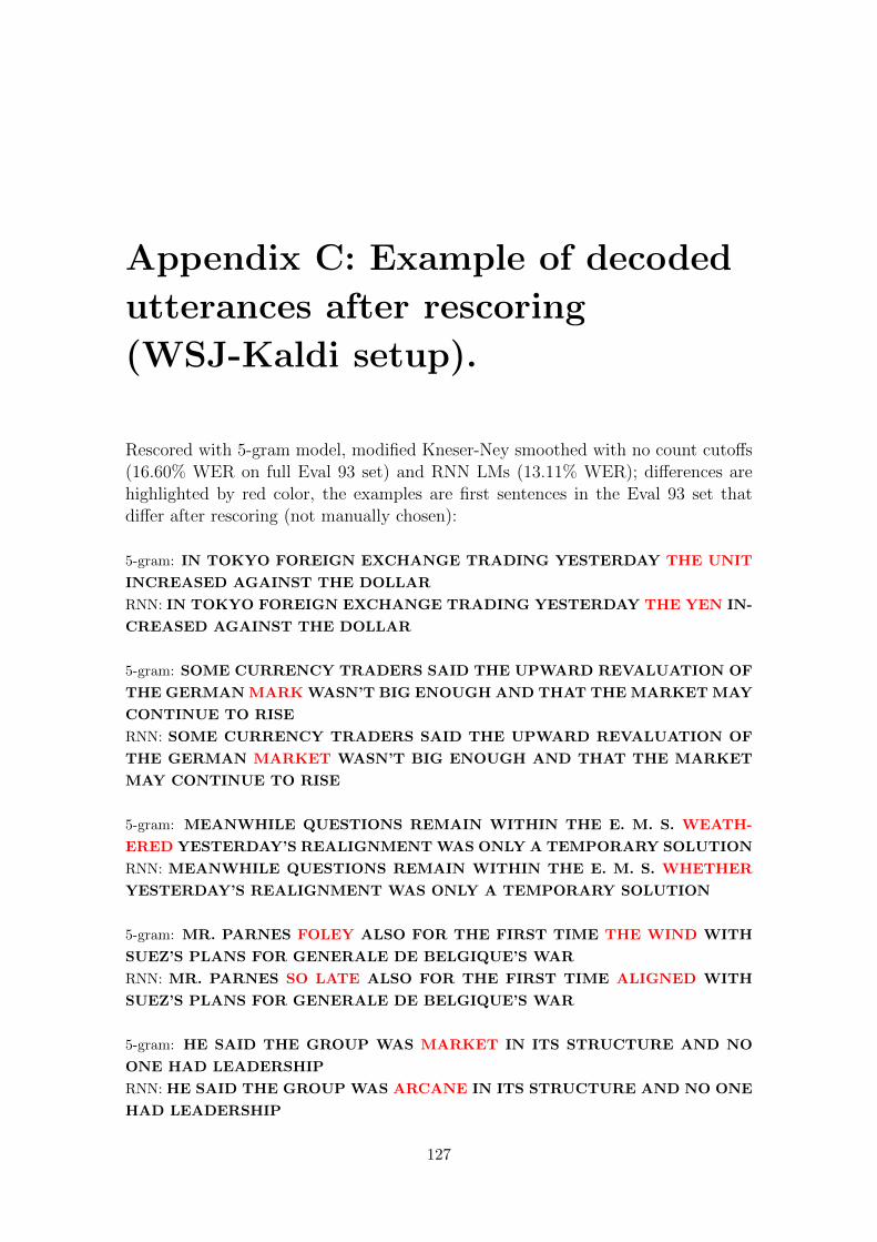
Appendix C: Example of decoded
utterances after rescoring
(WSJ-Kaldi setup).
Rescored with 5-gram model, modified Kneser-Ney smoothed with no count cutoffs(16.60% WER on full Eval 93 set) and RNN LMs (13.11% WER); differences arehighlighted by red color, the examples are first sentences in the Eval 93 set thatdiffer after rescoring (not manually chosen):
5-gram: IN TOKYO FOREIGN EXCHANGE TRADING YESTERDAY THE UNIT
INCREASED AGAINST THE DOLLAR
RNN: IN TOKYO FOREIGN EXCHANGE TRADING YESTERDAY THE YEN IN-
CREASED AGAINST THE DOLLAR
5-gram: SOME CURRENCY TRADERS SAID THE UPWARD REVALUATION OF
THE GERMAN MARK WASN’T BIG ENOUGH AND THAT THE MARKET MAY
CONTINUE TO RISE
RNN: SOME CURRENCY TRADERS SAID THE UPWARD REVALUATION OF
THE GERMAN MARKET WASN’T BIG ENOUGH AND THAT THE MARKET
MAY CONTINUE TO RISE
5-gram: MEANWHILE QUESTIONS REMAIN WITHIN THE E. M. S. WEATH-
ERED YESTERDAY’S REALIGNMENT WAS ONLY A TEMPORARY SOLUTION
RNN: MEANWHILE QUESTIONS REMAIN WITHIN THE E. M. S. WHETHER
YESTERDAY’S REALIGNMENT WAS ONLY A TEMPORARY SOLUTION
5-gram: MR. PARNES FOLEY ALSO FOR THE FIRST TIME THE WIND WITH
SUEZ’S PLANS FOR GENERALE DE BELGIQUE’S WAR
RNN: MR. PARNES SO LATE ALSO FOR THE FIRST TIME ALIGNED WITH
SUEZ’S PLANS FOR GENERALE DE BELGIQUE’S WAR
5-gram: HE SAID THE GROUP WAS MARKET IN ITS STRUCTURE AND NO
ONE HAD LEADERSHIP
RNN: HE SAID THE GROUP WAS ARCANE IN ITS STRUCTURE AND NO ONE
HAD LEADERSHIP
127

5-gram: HE SAID SUEZ AIMED TO BRING BETTER MANAGEMENT OF THE
COMPANY TO INCREASE PRODUCTIVITY AND PROFITABILITY
RNN: HE SAID SUEZ AIMED TO BRING BETTER MANAGEMENT TO THE
COMPANY TO INCREASE PRODUCTIVITY AND PROFITABILITY
5-gram: JOSEPH A. M. G. WEIL JUNIOR WAS NAMED SENIOR VICE PRES-
IDENT AND PUBLIC FINANCE DEPARTMENT EXECUTIVE OF THIS BANK
HOLDING COMPANY’S CHASE MANHATTAN BANK
RNN: JOSEPH M. JAKE LEO JUNIOR WAS NAMED SENIOR VICE PRESIDENT
AND PUBLIC FINANCE DEPARTMENT EXECUTIVE OF THIS BANK HOLD-
ING COMPANY’S CHASE MANHATTAN BANK
5-gram: IN THE NEW LEE CREATED POSITION HE HEADS THE NEW PUBLIC
FINANCE DEPARTMENT
RNN: IN THE NEW LEE KOREAN POSITION HE HEADS THE NEW PUBLIC
FINANCE DEPARTMENT
5-gram: MR. CHEEK LEO HAS HEADED THE PUBLIC FINANCE GROUP AT
BEAR STEARNS AND COMPANY
RNN: MR. JAKE LEO HAS HEADED THE PUBLIC FINANCE GROUP AT BEAR
STEARNS AND COMPANY
5-gram: PURCHASERS ALSO NAMED A ONE HUNDRED EIGHTY NINE COM-
MODITIES THAT ROSE IN PRICE LAST MONTH WHILE ONLY THREE DROPPED
IN PRICE
RNN: PURCHASERS ALSO NAMED ONE HUNDRED EIGHTY NINE COMMODI-
TIES THAT ROSE IN PRICE LAST MONTH WHILE ONLY THREE DROPPED
IN PRICE
5-gram: ONLY THREE OF THE NINE BANKS SAW FOREIGN EXCHANGE PROF-
ITS DECLINED IN THE LATEST QUARTER
RNN: ONLY THREE OF THE NINE BANKS SAW FOREIGN EXCHANGE PROF-
ITS DECLINE IN THE LATEST QUARTER
5-gram: THE STEEPEST FALL WAS THE BANKAMERICA COURTS BANK OF
AMERICA A THIRTY PERCENT DECLINE TO TWENTY EIGHT MILLION
DOLLARS FROM FORTY MILLION DOLLARS
RNN: THE STEEPEST FALL WAS A BANKAMERICA COURT’S BANK OF AMER-
ICA A THIRTY PERCENT DECLINE TO TWENTY EIGHT MILLION DOLLARS
FROM FORTY MILLION DOLLARS
5-gram: A SPOKESWOMAN BLAMED THE DECLINE ON MARKET VOLATIL-
ITY AND SAYS THIS SWING IS WITHIN A REASONABLE RANGE FOR US
RNN: A SPOKESWOMAN BLAMES THE DECLINE ON MARKET VOLATILITY
128

AND SAYS THIS SWING IS WITHIN A REASONABLE RANGE FOR US
5-gram: LAW ENFORCEMENT OFFICIALS SAID SIMPLY MEASURE OF THEIR
SUCCESS BY THE PRICE OF DRUGS ON THE STREET
RNN: LAW ENFORCEMENT OFFICIALS SAID SIMPLY MEASURE THEIR SUC-
CESS BY THE PRICE OF DRUGS ON THE STREET
5-gram: IF THE DRY UP THE SUPPLY THE PRICES RISE
RNN: IF THEY DRY UP THE SUPPLY THE PRICES RISE
5-gram: CAROLYN PRICES HAVE SHOWN SOME EFFECT FROM THE PIZZA
SUCCESS AND OTHER DEALER BLASTS
RNN: CAROLYN PRICES HAVE SHOWN SOME EFFECT ON THE PIZZA SUC-
CESS AND OTHER DEALER BLASTS
129