statistical analysis of biomedical data
TRANSCRIPT

Statistical analysis of biomedical data
Dissertation
zur Erlangung des Doktorgrades
der Naturwissenschaften (Dr. rer. nat.)
der Naturwissenschaftlichen Fakultat II – Physik
der Universitat Regensburg
vorgelegt von
Andreas Jung
aus Munchen
Dezember 2003

Das Promotionsgesuch wurde am 17. Dezember 2003 eingereicht.Das Promotionskolloquium fand am 29. Januar 2004 statt.
Prufungsausschuss:
Vorsitzender: Prof. Dr. Werner Wegscheider1. Gutachter: Prof. Dr. Klaus Richter2. Gutachter: Prof. Dr. Gustav ObermairWeiterer Prufer: Prof. Dr. Matthias Brack

Meinen Eltern


Contents
Glossary iii
Introduction 1
1 Survey of the biomedical data sets 51.1 Anatomy and physiology of the human brain . . . . . . . . . . . . 51.2 Neuromonitoring . . . . . . . . . . . . . . . . . . . . . . . . . . . 91.3 Electro-Encephalography (EEG) . . . . . . . . . . . . . . . . . . . 16
2 Time series analysis 192.1 Introduction . . . . . . . . . . . . . . . . . . . . . . . . . . . . . . 192.2 Theory . . . . . . . . . . . . . . . . . . . . . . . . . . . . . . . . . 202.3 Application: Correlation between ... . . . . . . . . . . . . . . . . . 22
2.3.1 Invos on left and right hemisphere . . . . . . . . . . . . . . 222.3.2 Licox and Invos . . . . . . . . . . . . . . . . . . . . . . . . 272.3.3 Arterial blood pressure and oxygen supply . . . . . . . . . 292.3.4 Arterial blood pressure and intracranial pressure . . . . . . 30
2.4 Conclusions . . . . . . . . . . . . . . . . . . . . . . . . . . . . . . 32
3 Model of the haemodynamic and metabolic processes in thebrain 353.1 Introduction . . . . . . . . . . . . . . . . . . . . . . . . . . . . . . 363.2 Fluid dynamics . . . . . . . . . . . . . . . . . . . . . . . . . . . . 37
3.2.1 Assumption for the hydrodynamical model . . . . . . . . . 383.2.2 The compartments . . . . . . . . . . . . . . . . . . . . . . 393.2.3 Final set of equations . . . . . . . . . . . . . . . . . . . . . 423.2.4 Standard values . . . . . . . . . . . . . . . . . . . . . . . . 443.2.5 Validation of the model . . . . . . . . . . . . . . . . . . . . 46
3.3 Oxygen transport . . . . . . . . . . . . . . . . . . . . . . . . . . . 523.3.1 The blood . . . . . . . . . . . . . . . . . . . . . . . . . . . 523.3.2 The Krogh cylinder . . . . . . . . . . . . . . . . . . . . . . 543.3.3 Theory . . . . . . . . . . . . . . . . . . . . . . . . . . . . . 58
3.4 Validation: Theory ↔ Experimental data . . . . . . . . . . . . . . 62
i

ii Contents
3.5 Conclusions . . . . . . . . . . . . . . . . . . . . . . . . . . . . . . 68
4 Independent component analysis 694.1 Introduction . . . . . . . . . . . . . . . . . . . . . . . . . . . . . . 694.2 Basic theory . . . . . . . . . . . . . . . . . . . . . . . . . . . . . . 73
4.2.1 Probability theory . . . . . . . . . . . . . . . . . . . . . . 734.2.2 Information theory . . . . . . . . . . . . . . . . . . . . . . 77
4.3 A geometric approach . . . . . . . . . . . . . . . . . . . . . . . . 814.3.1 Geometric considerations . . . . . . . . . . . . . . . . . . . 814.3.2 The (neural) geometric learning algorithm . . . . . . . . . 834.3.3 Theoretical framework for the geometric ICA algorithm . . 854.3.4 Limit points of the geometric algorithm . . . . . . . . . . . 874.3.5 FastGeo: A histogram based algorithm . . . . . . . . . . . 904.3.6 Accuracy and performance of FastGeo . . . . . . . . . . . 924.3.7 Higher dimensions . . . . . . . . . . . . . . . . . . . . . . 984.3.8 Conclusions . . . . . . . . . . . . . . . . . . . . . . . . . . 99
4.4 An information theoretical approach including time structures . . 1014.4.1 Introduction . . . . . . . . . . . . . . . . . . . . . . . . . . 1014.4.2 Theory . . . . . . . . . . . . . . . . . . . . . . . . . . . . . 1034.4.3 Algorithm . . . . . . . . . . . . . . . . . . . . . . . . . . . 1054.4.4 Applications . . . . . . . . . . . . . . . . . . . . . . . . . . 1084.4.5 A new concept for ICA – independent increments . . . . . 1114.4.6 Conclusions . . . . . . . . . . . . . . . . . . . . . . . . . . 112
4.5 Application to biomedical data . . . . . . . . . . . . . . . . . . . 1134.5.1 Neuromonitoring data . . . . . . . . . . . . . . . . . . . . 1134.5.2 Electro-Encephalography (EEG) data . . . . . . . . . . . . 113
4.6 Conclusions . . . . . . . . . . . . . . . . . . . . . . . . . . . . . . 121
Conclusions and Outlook 123
A Mathematical tools and proofs 127A.1 Correlation in the frequency domain . . . . . . . . . . . . . . . . 127A.2 Proof: Uniqueness of geometric ICA . . . . . . . . . . . . . . . . . 129A.3 Proof: Existence of only two fixed points in geometric ICA . . . . 130
Bibliography 133
Dank 141

Glossary
ABP Arterial Blood PressureBSS Blind Source SeparationCbO2 Oxygen content in the bloodC(a|v)O2 Oxygen content in the (arterial|venous) bloodcdf cumulative distribution functionCSF Cerebrospinal FluidCT Computer TomographyDFT Discrete Fourier TransformECG Electro-CardiographyEEG Electro-EncephalographyHb DeoxyhaemoglobinHbO2 OxyhaemoglobinIC Independent ComponentICA Independent Component AnalysisICP Intracranial PressureInvos In-Vivo Optical SpectroscopyLicox Liquor OxygenationMABP Mean Arterial Blood PressureMTM Multi Taper MethodNMR Nuclear Magnetic ResonancePCA Principal Component Analysispti mean partial oxygen pressure in the tissuepbO2 partial oxygen pressure in the bloodp(a|v)O2 partial oxygen pressure in the (arterial|venous) bloodpdf probability density functionRMT Random Matrix TheorySbO2 Saturation of the blood with oxygenS(a|v)O2 Saturation of the (arterial|venous) blood with oxygenSNR Signal to Noise RatioSTFT Short Time Fourier TransformTSA Time Series Analysis
iii


Introduction
Recently, the development of computer applications in the field of life sciences,in particular for the clinical and biomedical environments, has gained increasingattention due to the promising results in the treatment of patients.
Today, the recording of the patient’s status in multivariate data sets is astandard procedure in everydays clinical life. Apart from the immediate evalua-tion of the data by the physicians, the (off-line) analysis by dedicated computerprocessing tools can be a valuable information source.
In the context of data analysis, the methods derived in different fields ofphysics raise the question of applying these well known methods to life sciences,in particular to biomedical data analysis: Is it possible to obtain a deeper un-derstanding of the data with new (non)linear methods and physical models de-scribing the biological system? Can we further improve the analysis to reveal thehidden information in biomedical data by developing new algorithms overcominglimitations of the existing methods?
At the university hospital in Regensburg, the department of neurosurgeryrecords different biomedical data sets in the clinical environment. These record-ings have motivated this work and we will focus on two of these data sets. Onone hand, neuromonitoring data is recorded on the intensive care unit from pa-tients with severe head injuries. These data sets reflect mainly the followingbrain status parameters: oxygen content in the blood and tissue of the brain, thearterial blood pressure and the internal brain pressure. In addition, the patient’sbrain temperature is measured. On the other hand, the neural brain activityof patients is recorded in the electro-encephalography (EEG), in particular in thepost-operative treatment, to monitor neurological diseases. These recordings rep-resent – in contrast to the neuromonitoring data – highly multivariate data setswith 21 or more signals.
The questions arising in the analysis of the data are very diverse. They allfocus on a deeper understanding of the mechanisms of the investigated system,namely the human brain. In neuromonitoring data we may ask: Do the signalsinfluence each other, are they correlated in some sense? Which processes triggerthe system? What is the underlying biological system generating the signals? Inthe analysis of the EEG data we are mainly interested in whether new methodscan reveal more information or enhance the highly multivariate data.
1

2 Introduction
The techniques typically used in data analysis can be divided into three dif-ferent categories. This depends on the amount of knowledge available about theinvestigated system:
• Time Series Analysis:No knowledge is available about the system, only the time series originat-ing from the outputs of the system can be analysed. Two main techniquesare used: either unimodal (fourier transforms, wavelets, (non)linear anal-ysis using time embedding) or bimodal analysis methods (correlations andcouplings using nonlinear statistics). Symptoms or phenomena detectablein the time series can be quantified in such a way that statistical tests canbe applied.
• Independent Component Analysis (ICA):Hidden sources are underlying the measured signals. ICA is in particularuseful for the analysis of highly multivariate data sets ( 2 signals). Usingthe concept of ICA, the recorded signals can be described by a (non)linearmixing of unknown statistically independent sources.
• Model:The basic mechanisms describing the system are known. Based on thisknowledge, the behaviour of the system can be modeled, however some freeparameters have to be fitted by comparing the simulations to the measuredsignals. Properties of the system can be analysed by a sensibility andstability analysis including their parameter dependence. The reaction ofthe system with respect to parameter drifts, external influences etc. can beextrapolated to make possible ”predictions”.
With the methods listed above, using complementary approaches with verydifferent assumptions on the knowledge about the system, we will try to revealthe mechanisms generating the recorded signals and show how, for the variousdata sets, different methods have to be applied.
First, the reader will be made familiar with the basic anatomy of the humanhead including a description of the fluid dynamical and metabolic (oxygen supply)processes. Furthermore, a detailed description of the data sets and the basic phys-ical principles of the measurement methods will be presented. Finally, the originof the neural activity, their recording on the scalp with electro-encephalography(EEG) and their typical waveforms will be described in the first chapter.
The second chapter focuses on the analysis of the neuromonitoring data usingtime series analysis. To gain basic information about possible interconnectionsbetween the time series, a correlation analysis in the frequency domain will beused, to ensure that all processes are treated equally, independent of their ori-gin and their frequency band. Beside the well established correlations between

Introduction 3
the oxygen supply processes, more surprising couplings are found. In particularconnections between the arterial blood pressure, as a hydrodynamical process,and the oxygen content in the blood and brain tissue, as a metabolic process, areseen. First explanations of these observed correlations can be given with someintuitive descriptions using basic knowledge about the biological mechanisms inthe human brain.
In a more global context in chapter three, the results of the time series anal-ysis can be understood in more detail by using biomedical knowledge about thehuman brain. Based on this knowledge, we develop a model combining the fluiddynamical processes with a description of the oxygen supply in the human braintissue. Thereby, the amount of blood flowing through the brain, the so-calledcerebral blood flow, represents the main connection between the hydrodynamicaland oxygen supply model. One advantage of the model is that this parameter,which is in practice hardly measureable, can be numerically estimated and there-fore provides the physicians with important information about the patient’s state.Furthermore, this combined model allows to calculate all other parameters mea-sured in neuromonitoring, in particular the values describing the oxygen supplyprocesses. Based on a pure physical description, such a combined model enablesus to describe and understand in a more detailed way the couplings identified inthe time series analysis.
Furthermore, the influence of variations of the model parameters, i.e. the stateof health of the patient, on the evolution of the recorded brain status parameterscan now be described and can provide suggestions for the treatment of patients invarious situations. Interestingly, the relationship between some of the parametersobtained from the model show a surprisingly well established linear correlation,although the physical processes are highly complex and nonlinear. This obser-vation explains, why the linear correlation analysis of the time series producedsuch good results.
Before the investigation of the applicability of the independent componentanalysis (ICA) to biomedical data, an elaborate theoretical presentation of themethod will be given in chapter four. Two new algorithms will be presented. Firstan intuitive approach where geometrical consideration of the transformation ofscatter plots will be used to develop a theoretical framework. From these con-siderations, a fast histogram based algorithm (FastGeo) is derived. The secondalgorithm (FastTeICA) shows how time structures in the data can be includedin the framework of ICA by using methods known in time series analysis – inparticular by using independent time embedding vectors.
Finally, we present the results of the application of ICA to two biomedicaldata sets, namely the neuromonitoring data and the data recorded by electro-encephalography (EEG). The examples demonstrate both the power and theweakpoints of the concept based on ICA. In particular the interpretation of theextracted independent components have to be considered in real world applica-tions from a biomedical point of view.

4 Introduction
In the last chapter, the conclusions of the preceding chapters will be sum-marised and an outlook to further developments in the field of biomedical dataanalysis will be given.
This work was conducted in close cooperation with the department of neuro-surgery of the university hospital in Regensburg.

Chapter 1
Survey of the biomedical datasets
At the neurosurgery department of the university hospital in Regensburg differentdata sets are recorded as a standard procedure for immediate evaluation and lateroff-line analysis. In this chapter a survey of these recorded data sets and themeasurement methods is presented.
In the following work two kinds of data sets are of primary interest: first theneuromonitoring data recorded at the intensive care unit from patients with severehead injuries and second the electro-encephalography (EEG) data used to monitorneurological diseases. Both data sets consist of multi-channel recordings oftenreferred to as multivariate measurements. Before going into a detailed descriptionof the data sets and the measurement methods, an introductory overview of theanatomy and physiology of the human brain is given.
1.1 Anatomy and physiology of the human brain
As an introduction to this chapter, a survey of the anatomy and physiology of thehuman head will be given. Two schematic illustrations in figure 1.1 visualise thetwo main fluid circulations in the head, the cerebral blood flow (CBF) and thecerebrospinal fluid (CSF) flow. A further illustration in figure 1.4 shows a cross-section of the human head obtained by a nuclear magnetic resonance recordingof the authors brain.
The cranial bone which acts as a closed compartment accommodates thehuman brain. Between the cranial bone and the brain tissue, a fluid, the so-called cerebrospinal fluid, acts as a protection against external shocks.
The brain itself can be divided into two horizontal layers. The surface of thebrain is composed of nerve cell rich tissue which is called the gray brain matter(due to its colour) where the main neural activity of the brain takes place. Toconnect the nerve cells with each other throughout the brain, the subjacent tissue
5
6 Chapter 1. Survey of the biomedical data sets
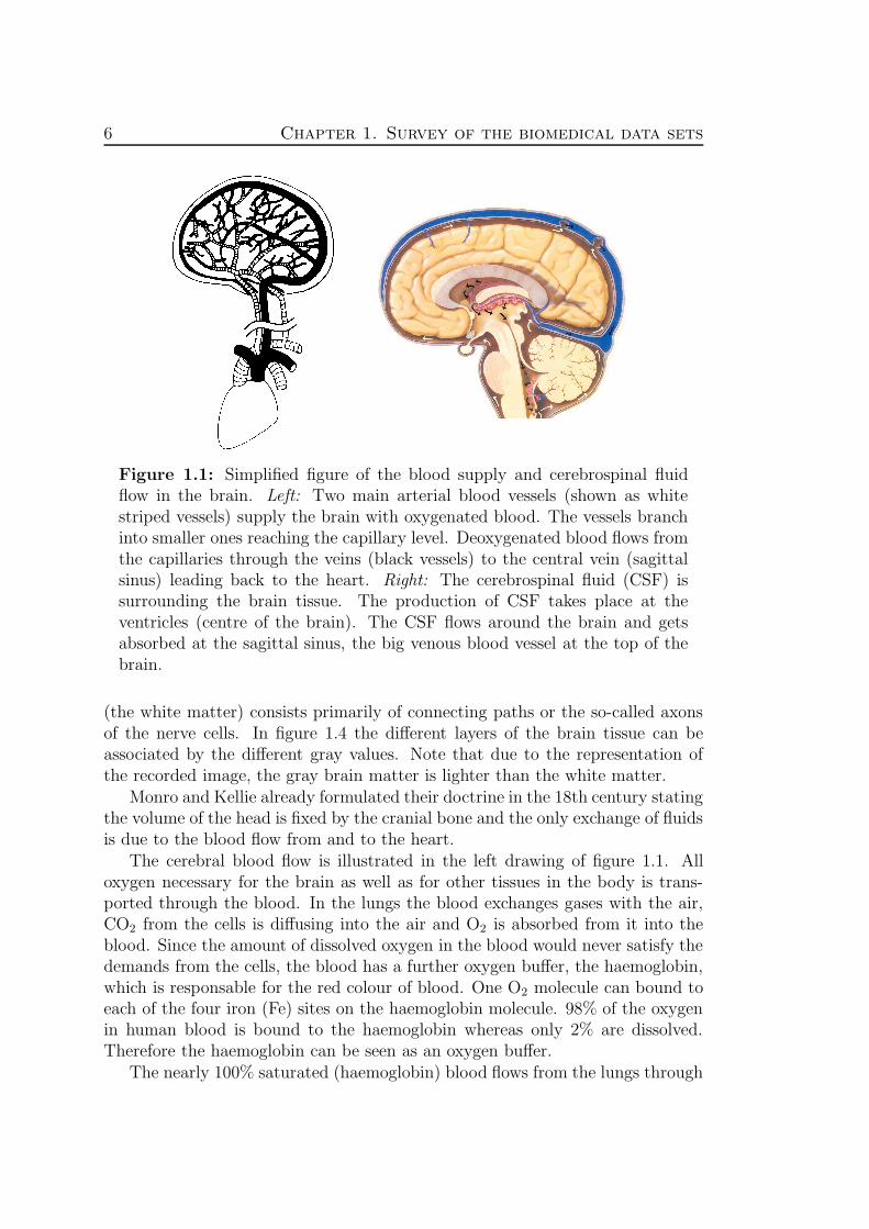
Figure 1.1: Simplified figure of the blood supply and cerebrospinal fluidflow in the brain. Left: Two main arterial blood vessels (shown as whitestriped vessels) supply the brain with oxygenated blood. The vessels branchinto smaller ones reaching the capillary level. Deoxygenated blood flows fromthe capillaries through the veins (black vessels) to the central vein (sagittalsinus) leading back to the heart. Right: The cerebrospinal fluid (CSF) issurrounding the brain tissue. The production of CSF takes place at theventricles (centre of the brain). The CSF flows around the brain and getsabsorbed at the sagittal sinus, the big venous blood vessel at the top of thebrain.
(the white matter) consists primarily of connecting paths or the so-called axonsof the nerve cells. In figure 1.4 the different layers of the brain tissue can beassociated by the different gray values. Note that due to the representation ofthe recorded image, the gray brain matter is lighter than the white matter.
Monro and Kellie already formulated their doctrine in the 18th century statingthe volume of the head is fixed by the cranial bone and the only exchange of fluidsis due to the blood flow from and to the heart.
The cerebral blood flow is illustrated in the left drawing of figure 1.1. Alloxygen necessary for the brain as well as for other tissues in the body is trans-ported through the blood. In the lungs the blood exchanges gases with the air,CO2 from the cells is diffusing into the air and O2 is absorbed from it into theblood. Since the amount of dissolved oxygen in the blood would never satisfy thedemands from the cells, the blood has a further oxygen buffer, the haemoglobin,which is responsable for the red colour of blood. One O2 molecule can bound toeach of the four iron (Fe) sites on the haemoglobin molecule. 98% of the oxygenin human blood is bound to the haemoglobin whereas only 2% are dissolved.Therefore the haemoglobin can be seen as an oxygen buffer.
The nearly 100% saturated (haemoglobin) blood flows from the lungs through

1.1. Anatomy and physiology of the human brain 7
Figure 1.2: Scheme of the behaviour of different blood vessels (arteries,capillaries and veins) related to their wall structure. The comparatively thickmuscular layer and high density of vasomotor nerves account for considerableconstriction and dilatation ability of cerebral arteries. These responses areless pronounced in the veins (especially in the cerebral veins, which are devoidof a continuous muscles layer), and absent in the capillaries (adapted fromMchedlishvili [1986]).
the arteries to the brain. The blood vessels branch into smaller and smaller vesselsuntil they reach the capillary level with diameters of only a few µm. Arteries areactive elements distinguishing themselves from the other blood vessels by havinga muscular layer around the vessel (for an illustration of the different blood vesselssee figure 1.2). This muscular layer comprises the brains possibility to regulatethe cerebral blood flow by dilating or constricting the arteries. The mechanismof keeping the CBF constant, the cerebral autoregulation, guarantees a steadysupply of oxygen over a wide range of the arterial blood pressure.
In contrast to the arteries, the capillaries are thin-walled vessels with typicallydiameters of 7 µm. The ratio of the surface of a capillary to the volume of thecontained blood is much higher at this level than at any other point in the bloodvessel arrangement. This enables the dissolved oxygen as well as other metabolicproducts like glucose to diffuse easily into the surrounding tissue. At the capillarylevel the main exchange of the metabolic products happens. But waste productslike CO2 can also diffuse from brain tissue back into the capillaries. The CO2
molecules can then be bind to the free Fe sites on the haemoglobin so that itcan transport the CO2 back to the lungs where it is again exchanged with a newO2 molecule. All diffusion processes, as for example between the blood vessels(capillaries) and the brain tissue or the air and the capillaries in the lungs, arebased on the pressure difference of the dissolved oxygen. Therefore the oxygendiffusion processes in the human body are a pure pressure depending processes.
8 Chapter 1. Survey of the biomedical data sets
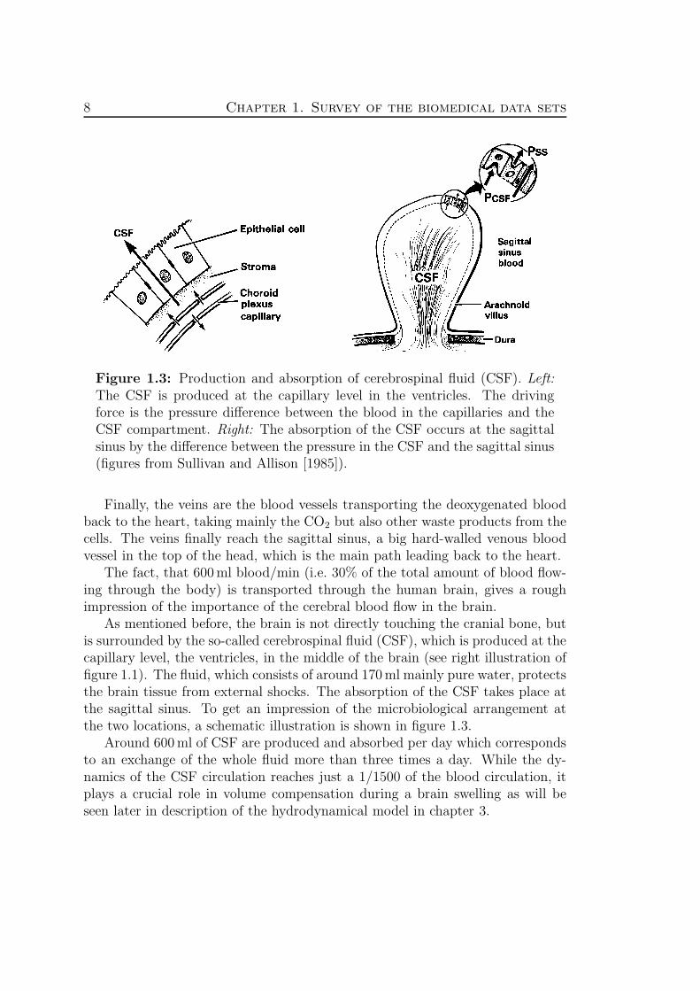
Figure 1.3: Production and absorption of cerebrospinal fluid (CSF). Left:The CSF is produced at the capillary level in the ventricles. The drivingforce is the pressure difference between the blood in the capillaries and theCSF compartment. Right: The absorption of the CSF occurs at the sagittalsinus by the difference between the pressure in the CSF and the sagittal sinus(figures from Sullivan and Allison [1985]).
Finally, the veins are the blood vessels transporting the deoxygenated bloodback to the heart, taking mainly the CO2 but also other waste products from thecells. The veins finally reach the sagittal sinus, a big hard-walled venous bloodvessel in the top of the head, which is the main path leading back to the heart.
The fact, that 600 ml blood/min (i.e. 30% of the total amount of blood flow-ing through the body) is transported through the human brain, gives a roughimpression of the importance of the cerebral blood flow in the brain.
As mentioned before, the brain is not directly touching the cranial bone, butis surrounded by the so-called cerebrospinal fluid (CSF), which is produced at thecapillary level, the ventricles, in the middle of the brain (see right illustration offigure 1.1). The fluid, which consists of around 170 ml mainly pure water, protectsthe brain tissue from external shocks. The absorption of the CSF takes place atthe sagittal sinus. To get an impression of the microbiological arrangement atthe two locations, a schematic illustration is shown in figure 1.3.
Around 600 ml of CSF are produced and absorbed per day which correspondsto an exchange of the whole fluid more than three times a day. While the dy-namics of the CSF circulation reaches just a 1/1500 of the blood circulation, itplays a crucial role in volume compensation during a brain swelling as will beseen later in description of the hydrodynamical model in chapter 3.

1.2. Neuromonitoring 9
1.2 Neuromonitoring
Throughout the treatment of a patient with a severe head injury at an intensivecare unit, different important physiological parameters are continuously moni-tored. A distinction is drawn between two different mechanisms which can bemonitored by sensing appropriate brain status parameters: first the cerebralmetabolism, i.e. oxygen supply and consumption in the brain tissue, and sec-ond the cerebral haemodynamics, i.e. the flow and the pressures of the cerebralfluids.
Primarily the oxygen supply of the brain is the most important factor formedical observation due to the fact that many of the patients die because ofoxygen undersupply. Therefore a constant monitoring of the patient is necessary.This monitoring or recording of the data is called ”neuromonitoring”.
Figure 1.4: Location of the neuromonitoring sensors – all sensors are placedat the front part of the brain. i) Licox: the sensor, measuring the partialoxygen pressure in the brain tissue (ptiO2) as well as the temperature, isplaced 2.7 cm deep into the brain matter. ii) Invos sensor: placed on thesurface of the scalp measuring the oxygen saturation of blood. The distance ofthe photodiodes to the infrared-LEDs is 3 and 4 cm. iii) ICP-sensor: localisedclose to the surface (1–2 cm depth) and measuring the intracranial pressure(internal brain pressure). Note: The image is an NMR measurement of theauthors brain :).
In figure 1.4 the usual positioning of the relevant neuromonitoring sensors isshown and will be described in the following:
• Cerebral metabolism – Two sensors are used for the measurement of theoxygen supply and consumption:

10 Chapter 1. Survey of the biomedical data sets
Licox (Liquor Oxygenation) is a brain tissue oxygenation monitoring sys-tem. This measurement method is a standard method in clinical applica-tions to monitor the supply of the brain tissue with oxygen. Due to thetemperature dependence of the measurement method the result need to becorrected by an integrated temperature sensor for a more accurate reading.Therefore the temperature values of the patients brain are also available.
Invos (In-Vivo Optical Spectroscopy) is a relatively new device to monitorthe oxygen supply in-vivo (i.e. in the living organism) without the need ofplacing a sensor into the patients brain tissue. The sensor is placed on thefront part of the scalp using infrared light to measure the oxygen contentof the blood (more precisely the degree of saturation of haemoglobin withoxygen).
• Cerebral haemodynamics – Mainly two parameters are monitored to getmore information about the flow and pressure of the cerebral fluids:
ICP (Intracranial Pressure) depicts the pressure inside the cranial bone.It is one of the most basic and important parameters recorded in standardneuromonitoring, since values above 40 mmHg are perilous. Long time mea-surements are done by a small piezo-electric sensor placed into the braintissue.
ABP (Arterial Blood Pressure) depicts the pressure of the artery blood,measured in the central arterial of the patient. Typically the mean arterialblood pressure (MABP) is given in the recordings with typical values in therange of 80 to 120 mmHg.
In the following sections, the basic physical principles of the measurementmethods will be described in more detail.
Licox including temperature measurement
The Licox sensor is placed into the brain tissue to measure the amount of availableoxygen for the nerve cells. The cells receive the oxygen by diffusion, this means,that the partial oxygen pressure in the tissue is proportional to the availableoxygen for the nerve cells. Measuring this value gives an indication of the oxygensupply of the brain tissue.
In figure 1.5 the basic configuration of a Licox sensor is shown. The sensor isbased on a polarographic Clark-type probe which is injected into the frontal partof the brain. Oxygen diffuses from the tissue through the polyethylene tube dif-fusion membrane into the inner electrolyte chamber filled with KCl. Between thepolarographic silver anode and gold cathode a current flows due to the appliedvoltage of a 800 mV. The measured current is proportional to the oxygen con-centration in the electrolytic chamber. Furthermore it is also proportional to theoxygen concentration in the surrounding tissue due to the diffusion membrane.

1.2. Neuromonitoring 11
Figure 1.5: Licox sensor: The basic design of the Revoxode ptiO2 probe isa polarographic Clark-type cell. (1)=polyethylene diffusion membrane (di-ameter of sensor is less than 1 mm), (2)=gold cathode, (3)=silver anode,(4)=electrolytic chamber (KCl) and (5)=brain tissue (figure adapted fromthe Gesellschaft fur Medizinische Sondentechnik mbH).
The chemical reactions at the silver and gold cathode – placed into a KClelectrolyte – are
• an oxidation at the gold cathode: O2 + 2 H2O + 4e− → 4 OH−
• a reduction at the silver anode: 4 Ag + 4 Cl− − 4e− → 4 AgCl.
As seen above, the chemical reaction with one O2 molecule results in a flow offour electrons through the circuit, i.e. the flowing current is proportional to theoxygen concentration.
Furthermore a temperature compensation is necessary for the Licox sensor,since the permeability of the membrane increases with temperature, permittingmore oxygen to enter the probe. The temperature measurement is done by an ad-ditional sensor in the probe and digitally processed in the Licox device. Thereforethe temperature values of the patients brain are also available.
In a typical Licox sensor, the surface of the diffusive membrane is about14 mm2 in size. Assuming a capillary density of around 300–1000 capillaries/mm2,the surface of the sensor touches hundreds of capillaries measuring therefore anaverage partial oxygen pressure. Still, compared to the size of the human brain,the sensor is measuring only a local oxygen concentration.
Typical measurement values of the Licox sensor are in the range of 10 mmHg to40 mmHg. Under special conditions (supply of the patient with 100% oxygen) thesensor measurements can reach values above 100 mmHg. Values below 10 mmHgare in general described as perilous.

12 Chapter 1. Survey of the biomedical data sets
Invos
The Invos sensor measures the percentage of oxygen saturated haemoglobin inthe blood. This type of measurement is called ”oximetry”.
It was discovered in the 1860’s that the coloured substance in blood, thehaemoglobin, is also its carrier of oxygen. Haemoglobin is a protein which isbound to the red blood cells and can bind oxygen to its 4 Fe (iron) sites. Atthe same time, it was noticed that two common forms of the molecule, oxidisedhaemoglobin (HbO2) and reduced haemoglobin (Hb), have significantly differentoptical spectra in the wavelength range from 600 nm to 1000 nm (see figure 1.6).The oxygen chemically combined with haemoglobin inside the red blood cellsmakes up nearly all of the oxygen present in the blood, only a small amount ofaround 2% is dissolved in the plasma.
10
100
1000
10000
100000
200 300 400 500 600 700 800 900 1000
Mol
ar A
bsor
ptio
n C
oeffi
cien
t [m
m-1
/mol
]
Wavelength [nm]
HbHbO2
730 nm805 nm
Figure 1.6: Absorption spectra of haemoglobin in deoxygenated (Hb) andoxygenated (HbO2) state. The Invos sensor is using two different wavelengths(730 and 805 nm) to distinguish between these two states and to calculatetheir ratio. At 805 nm the absorption of Hb and HbO2 is nearly equal incontrast to the absorption at 730 nm.
The functional principle of the Invos sensor is based on the difference inthe optical spectra of Hb (deoxyhaemoglobin) and HbO2 (oxyhaemoglobin), bysending light of two different wavelengths through the tissue and measuring theirabsorption. The tissue itself is relatively transparent in the range between 650 and1100 nm. Therefore the wavelengths λ1 = 730 nm and λ2 = 805 nm are chosenfor the oxymetric measurements by the Invos sensor. With the Beer-Lambert law(I = I0 e−αcl) we obtain two equations for the intensities at the two wavelength

1.2. Neuromonitoring 13
λ1 and λ2:
ln(I(λ)
I0(λ)) = −αHb(λ) · cHb · l − αHbO2(λ) · cHbO2 · l − t, (1.1)
with λ = λ1, λ2
where α is the absorption coefficient of Hb and HbO2, c their unknown concen-trations, l the length of the light path through the tissue and t = αt · ct · l theabsorption of the tissue which does not depend on the wavelength and oxygencontent, but is also unknown. To actually determine the concentration ratio be-tween Hb and HbO2, either a further measurement at a wavelength λ3 is neededor the mean absorption of the tissue t is directly determined in a separate ex-periment. Ignoring absorption and scattering in the tissue would lead to wrongvalues, since 83% of the light is attenuated by tissue as shown by Kauper [1999].
The saturation of HbO2 is then given by the ratio of the concentration ofHbO2 to the sum of the concentrations of haemoglobin
HbO2 saturation =cHbO2
cHb + cHbO2
(1.2)
which takes typically values in the range between 60% and 80%. However, Metz[2001] emphasised with his knowledge from clinical studies that rather the varia-tion of the values of the Invos sensor can indicate an oxygen undersupply of thebrain, a so-called ischemia, than the absolute value. Therefore in the analysis ofthe Invos data we will focus mainly on its dynamical aspects.
Furthermore, the use of two photodiodes with different distances from the lightemitting diodes (LED) can help to remove the surface effects and to calculate onlythe HbO2 saturation in the deeper areas of the brain. Calculations on the lightpaths of the infrared light through the scalp, the cerebrospinal fluid and the braintissue were done by Okada et al. [1997]. It was shown, that for smaller distancesbetween infrared LED and photodiode the light travels more through the scalpand the cerebrospinal fluid, while for distances above 4 cm, the photons travelmore through the brain tissue. When ”subtracting” the two measurements fromeach other, primarily the contribution from the deeper brain tissue is obtained.Using these results, a good balance between the removal of surface effects anda too strong absorption is achieved for a separation of 3 and 4 cm between theinfrared LED and photodiode, as used by the Invos sensor.
The actual value given by this sensor will reflect therefore the local averagedsaturation of the cerebral blood with oxygen. Generally it is assumed, that thecerebral tissue contains approximately 75% of venous and only 25% of arterialblood, as was also stated in a publication by Kim et al. [2000]. Therefore theHbO2 saturation measured – also abbreviated by SbO2 – is given by
SbO2 = 0.25 · SaO2 + 0.75 · SvO2 (1.3)

14 Chapter 1. Survey of the biomedical data sets
where SaO2 respectively SvO2 is the HbO2 saturation in the arterial and venousblood.
Finally, a discussion about the relation between the Licox and the Invos sen-sors and their measured values will be given in great detail in chapter 3.3.
Intracranial pressure and arterial blood pressure
The intracranial pressure (ICP) is measured in the brain tissue using the piezo-resistive effect. A membrane attached to the piezo element is exposed on oneside to the brain tissue, on the other side to the (external) air pressure. Thepressure difference measured at the element gives the intracranial pressure (ICP)value. Typical values range between 5 mmHg and 20 mmHg. Every value above40 mmHg is perilous.
Equivalent methods are used for the measurement of the arterial blood pres-sure. The sensor is normally placed in the central artery of the patient. Forthe analysis, only the mean long time behaviour of the arterial blood pressureis of interest. Therefore only the time average is given in the recordings, whichis abbreviated by MABP (mean arterial blood pressure) or often just by ABP.Typical MABP values are in the range between 80 to 120 mmHg, the true highresolution curve of the blood pressure pulse can of course take values between 60and 200 mmHg.
An example of neuromonitoring data
A typical example of neuromonitoring data recorded at the intensive care unitof the department of neurosurgery (university hospital Regensburg) is shown infigure 1.7. The data presented are the unfiltered (raw) time series from a 30 hoursrecording. In principle, the recordings of the patients parameters can be takenover any length in time with a sampling interval of up to one second. Our longestcontinuous measurement is a 6 days recording.

1.2. Neuromonitoring 15
12:00 18:00 00:00 06:00 12:00 18:00 00:0040
50
60
70
80
HbO
2 (rig
ht)
[%]
12:00 18:00 00:00 06:00 12:00 18:00 00:0040
50
60
70
80
HbO
2 (le
ft) [%
]
12:00 18:00 00:00 06:00 12:00 18:00 00:000
10
20
30
40
p tiO2 [m
mH
g]
12:00 18:00 00:00 06:00 12:00 18:00 00:0034
35
36
37
38
tem
pera
ture
[C]
12:00 18:00 00:00 06:00 12:00 18:00 00:0050
60
70
80
90
100
110
120
time [hours]
AB
P [m
mH
g]
12:00 18:00 00:00 06:00 12:00 18:00 00:005
10
15
20
25
30
35
40
ICP
[mm
Hg]
Figure 1.7: Recording of neuromonitoring data from the intensive care unitat the department of neurosurgery (University hospital Regensburg). The twoupper plots show the parameters of the cerebral metabolism: the saturationof the haemoglobin with oxygen (HbO2) in the left and right hemisphere ofthe brain, the partial oxygen pressure in the brain tissue (ptiO2) and thebody temperature of the patient. The lower plot shows the haemodynamicparameters: the mean arterial blood pressure (ABP) and the intracranialpressure (ICP). A section of only 30 hours of unfiltered data (sampling every15 seconds) is shown but recordings of up to 144 hours = 6 days are alsoavailable.

16 Chapter 1. Survey of the biomedical data sets
1.3 Electro-Encephalography (EEG)
The recording of electrical patterns at the surface of the scalp which primarily re-flect cortical electrical activity or ”brainwaves” is called electro-encephalographyand abbreviated by EEG1. In 1929, Hans Berger was the first who discovered thattiny rhythms of electrical wave activity could be detected at the human scalp.
In the following years typical potentials and rhythms of patients sufferingfrom epilepsy were categorised. In 1945 the first multi-channel recording withfour channels has been achieved. Quickly the electronic equipment developed to astandard 21 channel recording, called the Ten-Twenty-System. It was introducedas a standardised layout for EEG measurements in 1958 (see figure 1.8). Todayup to 256 channels are used for scientific research.
Figure 1.8: Location of the electrodes in the ten-twenty-system (21 chan-nels) which is the international standard for EEG measurements in clinicalapplication since 1958 (left=side-view and right=top-view of the patientshead). The positions are chosen to cover the whole scalp and make a loca-tion of a potential anomaly as good as possible (adapted from Kugler [1981]and Zschocke [1995]).
The EEG equipment consists of small, non-invasive electrodes which areplaced carefully with paste or a glue-like substance on a patient’s scalp. Lowvoltage signals (5–500 microvolts) are amplified and recorded with sampling ratesusually around 166 Hz by the EEG equipment. The measured potentials origi-nate from the nerve cells which generate electric potentials by chemical processes.Due to the huge number of nerve cells in the cortex of the brain, the measuredsignal is the sum of a huge collection of nerve cells.
The recordings are mostly taken with the eyes closed to get an undisturbedEEG, although the patient is sometimes asked to open them for short periods.
1Electro-encephalograph: electro=electrical; encephalon=head; graph=drawing/picture
1.3. Electro-Encephalography (EEG) 17
A typical recording time with eyes closed would be about 5 minutes. For anillustration, a sample of 6 seconds is shown in figure 1.9. The evolution of theelectric potentials at the electrodes over time is shown for all 21 channels. Byvisual inspection the neurosurgeon can identify four clinically relevant spectralbands: the delta (0–4 Hz), theta (4–8 Hz), alpha (8–12 Hz), and beta (above12 Hz) waves. A very dominant signal in closed eyes condition is the alpha waveactivity, which is easily identifyable also in the example shown here.
Today the EEG measurements are used in clinical applications to monitor neu-rological diseases. The method turns out to be often more sensitive for epilepsyand tumour evolution studies than computer tomography (CT) and nuclear mag-netic resonance (NMR) imaging. At the university hospital in Regensburg in par-ticular the tumour evolution after a neurosurgical operation is of interest. Patho-logical regions show typically an increase of slow activity (delta, theta waves) anddiminishing fast activity (alpha, beta waves).
In general, EEG interpretation requires considerable skill and often years ofclinical experience due to the complex structure of the signals. Therefore anautomatic detection and removal of artifacts could enhance the interpretation ofan EEG and the identification of potential neurological diseases. An example ofa typical artifact can be seen in channel ”Fp2” in figure 1.9 which correspondsto an eye movement or an eye blink.

18 Chapter 1. Survey of the biomedical data sets
61 62 63 64 65 66 67
A2
A1
Pz
Cz
Fz
T6
T5
T4
T3
F8
F7
O2
O1
P4
P3
C4
C3
F4
F3
Fp2
Fp1
time [s]
elec
tro−
ence
phal
ogra
phy
(EE
G)
− c
hann
el
Figure 1.9: An electro-encephalography (EEG) measurement from a pa-tient recorded at the department of neurosurgery (University hospital Re-gensburg). The EEG-channels are labelled by a abbreviation which corre-sponds to a given electrode on the head of the patient (see figure 1.8). Theplotted lines show the evolution of the electric potentials at each electrodeover time. One clear artifact (an eye-blink) is visible in channel ”Fp2”, fur-thermore the alpha-wave activity of the brain (∼ 8 Hz) is visible in nearly allchannels.

Chapter 2
Time series analysis
Typically, when applying time series analysis, only little knowledge is availableabout the system to be investigated. The only information source are the ”out-puts”, i.e. the time series recorded from the system. All information is gained bythe analysis of these outputs.
In this chapter we will use time series analysis to gain more information aboutthe interrelation between the different time series recorded in neuromonitoring. Itwill be shown that in particular the correlation in the frequency domain containsvaluable information which leads to a better insight into intracranial dynamics.
2.1 Introduction
Time series analysis is typically used for uni- or bimodal signals, that meansanalysing a system just by using one respectively two time series of the system.Neuromonitoring data is in contrast to EEG data a good candidate for the timeseries analysis. In particular the coupling between the time series of the neu-romonitoring data is of interest and can be treated by the so-called correlationanalysis. In the following a short overview over the two main techniques in timeseries analysis is given.
Nonlinear unimodal time series analysis is mainly based on a method calledtime-embedding as described by Kantz and Schreiber [1997]. It can be shown thatby analysing time delayed samples of one time series and plotting them in (2n+1)dimensions, it is possible to unfold the attractor of a n-dimensional system. Suchan analysis was also performed on the data of the neuromonitoring recordings,but it yielded no results. This was mainly due to two reasons. Firstly the highnoise level and the short length of the recorded data, which makes it hard tounfold the attractor of the system – as was also shown in the diploma thesis byMeier [2000] – and secondly the nonstationarity of the underlying system. Thesystem parameter in the background can change on the same time scale as thevariations of the system itself. Such conditions make the application of unimodal
19

20 Chapter 2. Time series analysis
time series analysis nearly impossible.Bimodal time series analysis concentrates more on the correlation or coupling
between two time series. The question to be answered is: Which signals have com-mon information contents and do they influence each other? Correlation analysisand higher order statistics like mutual information and conditional entropy, e.g.transfer entropy, can help to reveal such interconnections.
The problem in neuromonitoring focuses in particular on the signals triggeringthe system. To solve this question, the transfer entropy could be applied, since itcan find the direction and coupling strength between two processes as describedby Kaiser and Schreiber [2002]. But the high noise level and the nonstationar-ity of the data makes it nearly impossible to apply such methods. Further thetime synchronisation between the time series of the neuromonitoring data is notguaranteed. The measurement devices for the metabolic brain status parametersuse different non-synchronised clocks. Due to this fact, an absolute time stampwas not available and an estimation of coupling directions of the biological orphysical processes is therefore difficult. This problem will be solved in the futureby using radio controlled synchronised clocks.
In the following analysis we will therefore only use the correlation analysis,since it works more stable with noisy and nonstationary data. To be able tointerpret the flow of information and the coupling directions, we will use ourbiological and medical knowledge about the system.
2.2 Theory
In the following sections the method for the calculation of correlations betweentwo time series will be presented. The straight calculation of the correlation intime domain can have some drawbacks. For example when large oscillations anddrifts are superimposed to the data or if the correlation of the high frequencycontent between the processes is of interest. Therefore the change from timedomain to frequency domain is an appropriate solution, since all frequencies aretreated equally.
Correlation in the frequency domain
The calculation of the correlation in the frequency domain is equivalent to thecorrelation in time domain after filtering the time series with the correspondingfrequency filter. In the appendix the formula for the correlation in the frequencydomain between two time series x(t) and y(t) in a rectangular frequency windowω1 to ω2 is derived as
cx,y =12
∫ ω2
ω1x∗y + xy∗ dω
√∫ ω2
ω1xx∗ dω
∫ ω2
ω1yy∗ dω
(2.1)

2.2. Theory 21
where x(ω) depicts the fourier transform of x(t). Note: The equation is onlyvalid for long time series with zero mean (〈x〉, 〈y〉 = 0).
It turns out, that the definition of the correlation of frequency filtered timeseries is equivalent to calculating the correlation between the (complex) fouriercoefficients in the corresponding frequency window. The fourier coefficients caneither be calculated by using a discrete fourier transform (DFT) or more advancedspectra estimation methods as for example the multi taper method (MTM) usedin the analysis of Brawanski et al. [2002]. A comparison of the two spectraestimation methods applied to the neuromonitoring data showed the same basicbehaviour. Therefore we will only present results obtained with the discretefourier transform.
To take the nonstationarity of long data sets into account, usually a windoweddiscrete fourier transform or often called short time fourier transform (STFT) isapplied. Such methods can give more insight into the variability of the correlationover time. The window length is chosen to be much smaller than the length of thefull time series. The data in the chosen window is then assumed to be stationary.
Smoothing data and removing drifts in time domain
For the removal of unwanted artifacts in time domain, the time series can beconvoluted with a kernel. This procedure is often called ”smoothing”. In par-ticular the removal of long term drifts and the smoothing of the discrete dataas well as removing the noise from the analog measurements is of interest forthe neuromonitoring data analysis. We can write the convoluted/smoothed timeseries x(t) as
xsmooth(t) =1
τ
∫ t+τ
t−τ
x(t′) · k(t′ − t
τ) dt′ (2.2)
with τ depicting the width of the kernel. Different kernels for the convolution canbe used, as for examples a rectangular (k(x) = 1
2) or parabolic (k(x) = 15
16(1−x2)2)
kernel, where x ∈ [−1, 1]. For the following analysis we will always choose theparabolic kernel, since its behaviour is smoother than the rectangular one.
Cross-correlation of two time series
To find the most probable time delay between two time series, the method ofcross-correlations is used. The time series are shifted in time relatively to eachother and the correlation is calculated for every time shift τ .
〈x(t)y(t + τ)〉 =
∫x(t) y(t + τ) dt (2.3)
The τ at which 〈x(t)y(t+τ)〉 has a maximum, denotes in practical applications themost probable time shift between the time series. This method will be applied inthe further analysis for two different purposes. If the time series are recorded by

22 Chapter 2. Time series analysis
the same measurement device, than the detected time delay τ between the timeseries can give an indication to the physical processes producing such a time shift.An interpretation using some basic biological and medical knowledge will thenbe possible. But if the time series were recorded by two different measurementdevices and no absolute time stamp was available, the detected time delay willgive no valuable information.
In general, any time shift between the signals should be removed before ap-plying the frequency correlation analysis. Ignoring this time delay would lead tovirtual phase shifts in the fourier coefficients and distortions in the correlations.A simple example for this phenomenon is the shifting of two sinusoidal signalsby 1/4 of the period (corresponding to a phase shift of π/2). This shifting leadsto a correlation coefficient between the two signals of zero even if the signals aremeant to be highly ”correlated”.
2.3 Application: Correlation between ...
To analyse the recorded neuromonitoring data, i.e. Licox, Invos, arterial bloodpressure, intracranial pressure and the temperature, the method of correlation infrequency domain will be applied.
First analyses between the Invos and Licox data were performed by Brawanskiet al. [2002] showing the possible application of the method to neuromonitoringdata. In the following sections we will discuss all interesting correlations betweenthe recorded brain status parameters and give some indications to the origin ofthe observed phenomena. Explanations of the phenomena will be discussed inmore detail in chapter three when a model for the haemodynamic and metabolicprocesses in the brain is presented.
2.3.1 Invos on left and right hemisphere
First of all we will investigate the data from the Invos sensor on the left and righthemisphere to test on one hand the reliability of this measurement method andon the other hand to show in detail the analysis techniques used in this chapter.All further analysis of the neuromonitoring data will be done in the same way,but only the most important results are then presented.
The monitoring of patients at the intensive care unit with two Invos sensors toget an indication of the blood supply of both hemispheres is a standard procedure.Naturally we would expect an equal behaviour of the sensor data, but under somecircumstances as for example after a severe injury on one hemisphere or an injuryclose to the Invos sensor, differences can appear.
As an example, the raw data from an Invos measurement on the left andright hemisphere over a time period of 34 hours with a sample rate of 5 secondsis shown in figure 2.1.

2.3. Application: Correlation between ... 23
0 5 10 15 20 25 30 3540
50
60
70
80
time [hours]
HbO
2 (rig
ht)
[%]
0 5 10 15 20 25 30 3540
50
60
70
80
HbO
2 (le
ft) [%
]
Figure 2.1: Raw data from the Invos sensor on the left and right hemisphereof a patient. The relative saturation of the haemoglobin (Hb) with oxygen(O2) is plotted for both sensors over a period of 34 hours (samples every 5 s).
Time shift analysis
To determine the time shift between the time series of the Invos sensors, we usethe method of cross-correlation. The maximum of the correlation gives the mostprobable time delay. For these two data sets, which were recorded by the samemeasurement device, no time shift between the time series was detected. This isexpected since the Invos sensor measures the saturation of the haemoglobin withoxygen in the blood and as long as the blood supply of one of the hemispheres isnot impaired no time delay should be seen.
Power spectrum analysis
Further the power spectrum or more precisely the absolute value of the coefficientsof the fourier transformed time series can give an insight into the underlyingprocesses. Due to the spectral separation of different processes, we find twofundamental contributions in the Invos sensor data as shown in figure 2.2.
The typical one-over-f behaviour seen in many natural systems can also beidentified in the data from the Invos sensor. Further a white noise contributionas it is often seen as noise from measurement devices can be detected. One-over-ftime series, i.e. the power behaves as 1/f, are often interpreted as self-similar orfractal time series, because they show interesting fluctuations on many differenttime scales. A very intuitive introduction with many examples to this topic isgiven by Gardner [1978]. Compared to one-over-f noise, the white noise has apower spectrum of the time series which is independent of the frequency, i.e. equalpower in every frequency. A white noise contribution typically shows a completerandom behaviour in the time series.
The crossing of the two contributions occurs in the power spectrum at around2.5 mHz or a cycle length of 6 minutes. Above this frequency the white noise con-

24 Chapter 2. Time series analysis
10−2
10−1
100
101
102
102
104
106
108
1010
frequency [mHz]
pow
er [a
.u.]
Figure 2.2: Power spectrum of the Invos data shown in figure 2.1. Thepower is given in arbitrary units (a.u.) over the frequency using a doublelogarithmic plot. Two contributions can be identified: firstly the one-over-ftype signal (more accurate a 1
fα signal with α = 34) represented here as a line
with a negative slope and secondly a contribution of white noise (horizontalline). The intersection of both lines occurs at a frequency of ∼ 2.5 mHz or acycle length of ∼ 6 min.
tribution dominates the one-over-f behaviour. Interestingly the power spectrumsuggests that even for high frequencies the one-over-f noise contribution nevervanishes.
In the whole analysis of the neuromonitoring data, this phenomenon of twocontributions to the power spectrum is seen in all time series analysed.
Correlation in frequency domain
After having performed the analysis on the common behaviour of the data, thecorrelation between the time series in the frequency domain is investigated. Smallfrequency windows are taken for the analysis, usually 10 to 30 fourier coefficientsper window, to calculate the correlation between the time series. For a moreintuitive representation of the results a plot of the correlation over the cyclelength instead of the frequency is chosen in figure 2.3.
A clear difference can be seen between the correlation of the high and thelow frequency content. The Invos data is well correlated for cycle lengths above5 minutes (correlation coefficient is above 0.5), while for smaller cycle lengths thecorrelation breaks down and is negligible. Note, with statistical tests using whiteand coloured (time correlated) noise the level of the correlation coefficient for

2.3. Application: Correlation between ... 25
10−1
100
101
102
−0.4
−0.2
0
0.2
0.4
0.6
0.8
1
cycle length [min]
corr
elat
ion
Figure 2.3: Correlation in the frequency domain between the Invos signalsshown in figure 2.1. Every point corresponds to the correlation between ∼ 20fourier coefficients plotted at the mean cycle length of the chosen frequencywindow. Both Invos signals are significantly correlated (correlation coefficientabove the noise level of ∼ 0.5) for cycle lengths above 5 minutes. For longcycle lengths (> 2 h) as well as for high frequencies/short cycle lengths thecorrelation breaks down.
significantly correlated signals can be determined as shown in Brawanski et al.[2002].
Furthermore, a small drop of the correlation for very long cycle length isseen in the plot. This can be explained by the drifts of the sensors coming eitherfrom the sensor equipment itself or by possible changed environment in the tissuebeneath the Invos sensor.
Interestingly, the signal in the correlated frequency range (above 5 minutescycle length) corresponds to the one-over-f behaviour in the power spectrumplot (figure 2.2) which typically corresponds to the behaviour of natural systems.Further the crossing of the lines of the one-over-f noise and the white noise occursat around 5 minutes cycle length, where the power of the one-over-f signal is about10 times less then the one from the white noise. Tests with synthetic data haveshown a robustness of the correlation method down to a signal to noise ratio(SNR) of 1:10. This SNR corresponds exactly to the crossing of the two lines inthe power spectrum. Therefore, correlations between the two Invos signals in thehigher frequencies can not be excluded.
Reconstruction and filtering of the data
To get an impression of the waveform of the significantly correlated part of thesignals, the data can be reconstructed by using only the significantly correlatedfrequencies in the inverse fourier transform. The resulting signals of the Invos

26 Chapter 2. Time series analysis
sensor for the left and right hemisphere are shown in figure 2.4.
0 5 10 15 20 25 30 35−10
−5
0
5
10
time [hours]
∆ H
bO2 (
right
) [%
]
0 5 10 15 20 25 30 35−10
−5
0
5
10
∆ H
bO2 (
left)
[%]
Figure 2.4: Reconstructed Invos signals using only the significantly corre-lated frequencies shown in figure 2.3. This corresponds to a frequency filteringusing a rectangular window between 5 minutes and 2 hours.
Comparing these signals to the raw data (shown in figure 2.1), the removalof the noise and the drift by the reconstruction can clearly be seen. With thisknowledge, we could try to obtain similar data just by filtering or smoothingthe data in time domain using the kernel convolution method. Using a driftremoval method of ±2 hours (i.e. smoothing the data with a ±2 hours kernel andsubtracting this from the original data) gives the drift removed signal. Furthersmoothing the data with a ±2 minutes parabolic kernel, the signals shown infigure 2.5 are obtained.
0 5 10 15 20 25 30 35−10
−5
0
5
10
time [hours]
∆ H
bO2 (
right
) [%
]
0 5 10 15 20 25 30 35−10
−5
0
5
10
∆ H
bO2 (
left)
[%]
Figure 2.5: Raw data from the Invos sensors filtered in time domain usinga smoothing of ±2 min and a drift removal of ±2 hours. Filtering in time do-main shows the same result as the frequency filtered time series in figure 2.4.
It turns out that the signals from both Invos sensors (after applying the kernelconvolution/smoothing method) match even better than the ones obtained by the

2.3. Application: Correlation between ... 27
frequency reconstruction method. The deviations at the boundaries seen in thefrequency reconstruction are due to the sharp filtering in the frequency domainand disappear when using the time domain filtering.
Conclusions
From the theoretical point of view, we can assume to have a one-over-f processfrom the natural system (the patient) which is covered by white noise originatingfrom the measurement device (the Invos sensor). Filtering the data in timedomain using a ±2 hours drift removal and a ±2 minutes smoothing, we obtainreasonable data showing the correlated content of both Invos channels.
From the medical point of view we can conclude, that the Invos sensor is areliable measurement method, since the correlation between the time series isstable over long time periods. For the further analysis, we are only interestedin the variations (above 5 minutes) of the signals, since Metz [2001] already indi-cated that only the dynamics of the signals is of interest for the clinical analysis.Further, the long time drifts seem not to contain any valuable information andcan therefore be neglected.
2.3.2 Licox and Invos
After having presented the detailed analysis of the Invos data, the data fromthe two sensors measuring the oxygen supply of the brain is now analysed. Thepartial oxygen pressure in the brain tissue (measured by the Licox sensor) iscompared to the oxygen content in the blood or more precisely to the saturationof haemoglobin with oxygen in the blood (measured by the Invos sensor).
A correlation between the two parameters is expected since both sensors mea-sure the available oxygen for the nerve cells. First analyses have been done forpreviously recorded (Invos and Licox) data by Brawanski et al. [2002] where theauthors presented how advanced spectral estimation methods can be used tocalculate correlations between biomedical time series. The question on the com-mon information content between Invos and Licox could be positively answered,showing the stability of the correlation on a large group of patients.
Problems in the measurements of Licox and Invos can arise if they are placedtoo close to or into an injured tissue. In such a case no correlations between thesensors can be expected.
First the time shift between the signals is investigated. As described in theintroduction, the problem of time synchronisation can arise if two different mea-surement devices are used. For the pair of sensor signals analysed in this section,the devices were started at different points in time. Therefore any coupling di-rections or time delays due to processes in the brain, can not be investigated byusing the cross-correlation analysis. But for the further analysis the data wasaligned in time.

28 Chapter 2. Time series analysis
Performing the correlation analysis in the frequency domain on this timealigned data sets, the plot in figure 2.6 is obtained. As previously seen, the plotcan be divided into two main parts, the high frequency content (below 6 minutescycle length) which is not significantly correlated and a low frequency content(between 6 minutes and 3 hours) which is highly correlated. Therefore both sig-nals seem to have only common information down to a cycle length of 6 minutes.Possible correlations in the higher frequency range are either not resolvable bythe method or not existing. The breakdown of the correlation above 3 hours isagain due to the drifts respectively trends in the data.
10−1
100
101
102
−0.4
−0.2
0
0.2
0.4
0.6
0.8
1
corr
elat
ion
cycle length [min]
Figure 2.6: Correlation in the frequency domain between Licox and Invossignals based on continuous data of 27 hours. Both signals are significantlycorrelated (correlation coefficient above the noise level of ∼ 0.5) for cyclelengths above 6 minutes. For very long cycle lengths (> 3 h) as well as forhigh frequencies/short cycle lengths the correlation breaks down.
Overall the signals are well correlated over long time periods as was expectedand seen in previously recorded data. Still, the result of a linear correlation isan interesting fact for the description of the oxygen supply in the brain. Bothsensors are measuring in some sense the oxygen content in the brain, but theirmeasured values are connected by a nonlinear dissociation curve, the diffusionprocess and the cerebral blood flow as will be seen in chapter 3.3.
The actual variations of the signals are thought to be changes in the cerebralblood flow (CBF). The CBF depends on one hand on the arterial blood pres-sure (as will be shown in the next section) and on the other hand on additionalparameters influencing the arteries regulating the CBF.
Sometimes huge variations are seen in the data sets (mainly in the Licoxvalues) originating from a medical manoeuvre such as the cleaning of the airtube of the patient. The patient is then supplied with pure oxygen prior to themanoeuvre and therefore high oxygen values are measured.

2.3. Application: Correlation between ... 29
A detailed description of the relation between Licox and Invos, taking allphysical processes into account, is given in chapter 3.3.
2.3.3 Arterial blood pressure and oxygen supply
In this section we will focus on the connection between the haemodynamics, i.e.primarily the arterial blood pressure, and the oxygen supply, i.e. the measuredsignals from Invos and Licox. As shortly mentioned in the previous section, thevariations of the signals from the Licox and Invos sensors are assumed to be dueto variations of the cerebral blood flow. If more blood flows through the brain,more oxygen per time is available for diffusion into the tissue and therefore ahigher oxygen content should be measured.
The variations in the cerebral blood flow itself are expected to be due tothe variations in the arterial blood pressure (ABP) as a higher ABP leads to ahigher blood flow and in the end to a higher oxygen content in the tissue. Thisconnection between ABP and the values measured with the Licox respectivelyInvos sensor is investigated in the following.
Performing the same analysis as done in the previous sections, we obtain aclear correlation between the signals for selected parts of the data. Again a lookat the correlations in the frequency domain (see figure 2.7) gives an insight intothe possible processes.
10−1
100
101
102
−0.4
−0.2
0
0.2
0.4
0.6
0.8
1
corr
elat
ion
cycle length [min]
Figure 2.7: Correlation in the frequency domain between the arterial bloodpressure and the oxygen content in the brain tissue (Licox sensor). Theanalysis is based on continuous data of 21 hours. Both signals are significantlycorrelated (correlation coefficient above the noise level of ∼ 0.5) for cyclelengths above 10 minutes. For longer cycle lengths (> 1.5 h) as well as forhigh frequencies/short cycle lengths the correlation breaks down.

30 Chapter 2. Time series analysis
Noticeable is the small but clearly correlated region in the frequency domainranging from 10 minutes to just over one hour. Outside this range the correlationbreaks down quickly. On the low frequency end this can be explained by clearlyvisible trends in the data and on the high frequency end by either a high noiselevel and/or a damping mechanism from the brain.
The time shift for this pair of signals could be measured, because both mea-surements were simultaneously recorded by the same device. A cross-correlationanalysis shows that the variations of the arterial blood pressure are seen ∼135 seconds earlier than the ones from the Licox sensor. This can be explainedby two processes. Firstly by the reaction time (the so-called t90% time) of theLicox sensor of around 90 seconds and secondly by the time the blood needs toreach the capillaries and oxygen to diffuse into the tissue. From this knowledgewe can conclude that the arterial blood pressure must be the driving force of theseen variation in the data measured by the Licox sensor.
But as mentioned before, we can only see this correlation in parts of the datasets (less than 10% of the data). Later, during the discussion of the model, wewill learn that the autoregulation plays a major role in the correlation of theABP with the oxygen supply. Only if the autoregulation, i.e. the regulation ofthe blood flow by the brain’s arteries, is impaired, a correlation between ABPand Licox/Invos should be seen.
2.3.4 Arterial blood pressure and intracranial pressure
Focusing on the haemodynamics, we will now investigate the connection betweenthe driving force of the system, the arterial blood pressure, and the intracranialpressure, which is one of the most important brain status parameters monitoredon the intensive care unit. The relation between these two parameters is animportant factor to understand the hydrodynamic system in the brain.
The human head can be seen as a closed compartment in which the brain andthe intracranial fluid is contained. A local swelling in the brain can lead to anincrease of the intracranial pressure by a diminishment of the available volumeand therefore a compression of the brain tissue. The question to be asked, whenanalysing the sensor data, is, whether an increase of the arterial blood pressurecan lead to an increased intracranial pressure or not.
This connection could be expected, since the increase of the arterial bloodpressure leads to an increase of the (arterial) blood vessels and a reduction of theavailable volume in the brain. But this increase of volume can be compensatedby an increased absorption of the cerebrospinal fluid as described in the firstchapter.
In the analysis of more than 670 hours of data we could identify a sectionof 9 hours of continuous data showing a significant correlation. As usual, thecorrelation between the two time series is plotted over the cycle length of thecorresponding frequency window (figure 2.8).

2.3. Application: Correlation between ... 31
10−1
100
101
102−0.8
−0.6
−0.4
−0.2
0
0.2
0.4
0.6
0.8
1
corr
elat
ion
cycle length [min]
Figure 2.8: Correlation in the frequency domain between the haemodynam-ical signals: the arterial blood pressure and the intracranial pressure. Theanalysis is based on continuous data of 9 hours. A significant correlation(correlation coefficient above the noise level of ∼ 0.5) is only given for cyclelengths above 15 minutes. For shorter cycle lengths one can see a good cor-relation around 5 minutes, before it breaks down for high frequencies/shortcycle lengths.
Again the plot showing the correlation can be divided into two main parts.The high frequency content is not well correlated, except a few high peaks below1 minute cycle length which are probably artifacts of the measurement device.Whereas the low frequency content has a high correlation, in particular for cyclelengths above 20 minutes. To get a better impression of the actual waveform,the arterial blood pressure and intracranial pressure are plotted (after a filteringin the time domain) in figure 2.9. From the plotted time series, a very goodcorrelation of the larger and longer oscillations can be seen in contrast to theones on the smaller time scale.
Since both measurements are recorded with the same analog/digital converter,the time shift between the signals can be calculated. The variations of the ar-terial blood pressure are seen 30 seconds earlier than those from the intracranialpressure. This supports the hypothesis that the arterial blood pressure is thedriving force of the system.
As mentioned before, the correlation between the haemodynamic parameters(ABP and ICP) could only be seen very rarely (in 1.3% of the data). This willget more clear in chapter 3, where the model of the haemodynamic and metabolicprocesses in the brain is presented. We will see, that the ICP is stable, as long ascerebrospinal fluid (CSF) can be absorbed into the venous blood to compensatethe increased volume of the arteries and other blood vessels. Without CSF nocompensation is possible and a rise in the ABP is followed by an increasing ICP.

32 Chapter 2. Time series analysis
0 2 4 6 8 10−15
−10
−5
0
5
10
15
time [hours]
∆ A
BP
[mm
Hg]
0 2 4 6 8 10−5
0
5
∆ IC
P [m
mH
g]
Figure 2.9: Filtering the raw data from the arterial blood pressure and theintracranial pressure in time domain with a smoothing of ±2 min and driftremoval of ±4 h. The correlation of the long and big oscillations are clearlyvisible, in contrast to the short time oscillations which are not well correlated.This observation is in good agreement with the plot in figure 2.8.
Then, the arteries transmit the pressure directly to the brain tissue.From the medical documents and nuclear magnetic resonance images we can
support this theory. The cerebrospinal fluid was (up to a small amount) fullyabsorbed. The patient had a severe swelling of the brain, the scalp had to beopened to overcome a further increase of the brain pressure.
2.4 Conclusions
Concluding the results of this chapter, we distinguish between a theoretical anda medical part.
Focusing on the theory: With the correlation analysis in the frequency domainwe can extract a lot of valuable information. It seems that the signals are oftenlinearly correlated. Higher order statistics like mutual information or transferentropy seems not to be necessary to reveal higher order correlations. In precedingtests, these (higher order statistics) methods were also applied to the data, butshowed equivalent results. However, difficulties with the statistics arise, sincethese methods need longer time series with a better signal to noise ratio.
The analysis of the correlation in the low frequency range (variations above5 to 10 minutes) shows a high correlation between the signals. In the powerspectrum this frequency range corresponds to a one-over-f type noise behaviourwhich is typically seen in natural systems. The correlation in this frequencyrange seems to be a good measure on which statistical tests can be applied.This measure could therefore be used in future devices monitoring the patient.Changes in the correlation of the signals could indicate a variation in the patientscondition and raise an alert.

2.4. Conclusions 33
The drifts or trends in the time series (cycle length above 2 hours) seem notto contain any valuable information, no correlation is seen between these signals.Therefore we suggest to remove the drift in time domain by kernel-smoothing.But one exception should be mentioned here. The drift of the Licox sensor iscorrelated with the temperature seen in at least two data sets of 30 and 50 hours.An explanation for this correlation can not yet be given, since the Licox sensor istemperature compensated and calibrated. The phenomenon is still under inves-tigation by the company providing the Licox sensor, but maybe a physiologicalexplanation is more reasonable than a technical one.
Furthermore the signals below 2 minutes cycle length have either no commoninformation content or the method used in this analysis cannot resolve thesecorrelations. Still the typical one-over-f type behaviour is seen in this frequencyrange, even if it is covered by a dominating white noise process. Therefore wesuggest to smooth the data in time domain with a kernel of ±2 minutes.
From the medical point of view: The Invos sensor gives reproduceable andstable measurements over longer periods of time (34 hours – as shown in theexample above), but the placement of the sensor is important. When correctlyplaced (not too close to the injured tissue) the variations/dynamics of the datacan be trusted. The absolute values of the sensor are not always reliable due tounknown trends.
Under normal conditions we can also see stable correlations between Licox andInvos – in the example shown above on a period of 27 hours. The origin of theactual variations of the data values can be explained on one hand by variationsin the cerebral blood flow, which produces only small variations and on the otherhand by clinical manoeuvres (supply of the patient with air consisting of 100%oxygen) resulting in huge oscillations in the data. These phenomena are explainedin great detail in chapter 3.3.
The arterial blood pressure seems to be the driving force of the hydrodynamicrespectively the haemodynamic system if a disease is present. In the case of animpaired autoregulation (was seen only in less than 10% of the time) it can lead tothe coupling between the ABP and the Licox values due to the linear dependenceof the cerebral blood flow on the ABP. If a swelling of the brain is present, thenthe ABP couples also with the ICP due to the missing CSF to compensate thevolume changes (this was only seen very rarely in 1.3% of the time).


Chapter 3
Model of the haemodynamic andmetabolic processes in the brain
With the aid of biological and medical knowledge about the dynamical prop-erties of the brain – mainly the haemodynamic and metabolic (oxygen supply)processes – a global model for the dynamical behaviour of the system ”brain”can be designed.
Previous analysis methods only focused on parts of the system, using for ex-ample correlation analysis of the time series. With the capability of investigatingthe system using a model it should be possible to explain the observed phenomenawithin a global context.
The final goal of such an analysis is to find a model which can reproduceand explain all the measured data, i.e. the combination of haemodynamics andmetabolics. In this case it would then be possible to compare simulations ofthe model with the measured data – after fitting free parameters of the model.Deviations between the prediction of the model and the measured data couldindicate a possible change of the parameters i.e. the patients state of health.
In this chapter we propose a basic hydrodynamic model with realistic exten-sions to existing models which fits the needs of neurosurgical applications. In asecond step we will couple this to a newly derived model describing the meta-bolic processes in the brain. This will result in a new so-called combined model.The main connection between the two models is the cerebral blood flow which ishardly measureable in clinical applications over longer periods. Therefore this pa-rameter determined by the model can give valuable information to the physiciansfor the treatment of the patient.
In the following the fluid dynamical and the oxygen supply model will bedescribed in detail and validated on typical curves and measured data. It will getclear, how the observed phenomena seen in the previous section can be explainedwithin the context of this model.
35

36Chapter 3. Model of the haemodynamic and metabolic processes
in the brain
3.1 Introduction
In this chapter, first a hydrodynamical model based on interacting subunits, thecompartments, will be derived. Compartment models of the present type havea long history, dating back to the earliest of such models formulated by Monroand Kellie in the end of the 18th and begin of the 19th century using a threecompartment model (arterial, venous and brain tissue). More recent works on thistype of models are using an increased number of compartments and relaxationsof some assumptions. But many of these models lag of the correct description ofone or the other processes in the brain. Often, instead of a full description of theautoregulation processes, a constant blood flow is assumed or the compressibilityof the brain tissue is neglected (Kadas et al. [1997], Lakin et al. [1996]). For themodelling of the autoregulations, Czosnyka et al. [1992] and later Bekker et al.[1996] proposed the use of a pressure depending nonlinear resistance, regulatingthe blood flow. Extensions to the description of the capacitance of the bloodvessels and the brain tissue were then given in more detail by Czosnyka et al.[1997] and comparisons with measurements by Stevens [2000].
The model presented in this work will more closely follow the one proposedby Ursino and Lodi [1997], since it uses a more realistic description of the au-toregulation process and takes into account the possible collapse of the veins ina preliminary step. Still, some more consistent extensions will be presented here,in particular regarding the compression of the veins and using a simpler equationfor the autoregulation. Many basic concepts of the later works of Ursino werealready presented in the excellent paper from 1988 (Ursino [1988]).
After presenting a hydrodynamical model, which is adapted to the require-ments of neurosurgical applications, the details of the oxygen supply will bediscussed. Krogh [1918-1919] proposed as the first a model for the descriptionof the oxygen supply in tissue. An elaborated discussion of the literature andthe assumption of the Krogh cylinder is given in Reneau et al. [1967] as wellas results of numerical calculations. In the following years Reneau and otherspublished further works considering countercurrent flows and the undersupply oftissue (Reneau and Knisely [1971], Reneau et al. [1970], Hudetz et al. [1982]).Still, the derivation of the analytical expression for the mean oxygen pressure intissue, as measured by a device like the Licox sensor, and the oxygen contentin the blood, as measured by the Invos sensor, and in particular their relation-ship, were not presented in any works published. The reason for this is thatuntil a few years ago the data of both sensors couldn’t be recorded over longperiods. Therefore, the possibility to compare experimental measured data withtheoretical predictions was not existing.
In this work we will also show, which further difficulties have to be overcometo get a meaningful comparison of the absolute values of the predictions withmeasured data.

3.2. Fluid dynamics 37
3.2 Fluid dynamics
In this model approach, fluid and matter constituents within the human head aresubdivided into a number of interacting subunits, namely the compartments. Theinteractions are mainly determined by fluid dynamical processes. Basically theblood and the cerebrospinal fluid (CSF) will interact as separate flows betweenthe compartments, whereas the brain tissue will be depicted by one compartmentconsisting of soft matter.
The compartment model used in this work is presented in figure 3.1 showinga closed overall compartment with only one inflow and one outflow of blood. Allother fluid dynamical processes take place in this overall compartment. In thismodel we will distinguish between the following 7 compartments:
A - arteries, C - capillaries, V - veins, S - sagittal sinus, B - brain tissue,F - cerebrospinal fluid and E - extra volume describing swelling of brain tissue.
The details of each compartment will be discussed in the following sections.
RAC
ABC
RCV
VBCpA
pC p
V
pF
RC
F
qI
R VS
qS
pS
RFS
S
pB BC
qA
VAC
E
B
F
Figure 3.1: A hydrodynamical model describing the processes in the brainusing 7 distinguishable compartments: A - arteries, C - capillaries, V - veins,S - sagittal sinus, B - brain tissue, F - cerebrospinal fluid and E - extra volumedescribing swelling of brain tissue. For every compartment a pressure pX canbe defined as well as flows (qXY ) respectively resistances (RXY ) between thecompartments. Furthermore for volumes with a membrane a capacitanceCXY is defined.
To make it easier to specify for example the pressures in the compartmentsor the flows between compartments, the following conventions will be applied.For the pressure in compartment ”A” the variable pA will be used. When twocompartments are involved as for example the flow between compartment ”A”and ”C”, the variable qAC is used. To depict the standard value of a variable anindex n will be attached as for example qACn.

38Chapter 3. Model of the haemodynamic and metabolic processes
in the brain
The physical equation describing the hydrodynamical processes is based uponthe conservation of mass and reads as
∑qi =
dm
dt=
∂m
∂ρ︸︷︷︸=V
·∂ρ
∂t+
∂m
∂V︸︷︷︸=ρ
·∂V
∂twith m(t) = ρ(t) · V (t). (3.1)
The change of mass in the compartments depends on the fluxes in and out ofthe compartment (qi) as well as on the changes of the density ( ∂ρ
∂t) and on the
change of the volume of the compartment ( ∂V∂t
). For incompressible media, like
the fluids, ∂ρ∂t
is of course zero. Therefore the first term in (3.1) can be neglected.
3.2.1 Assumption for the hydrodynamical model
In the following, the assumptions for the compartment models used in this workare stated from which the equations are derived later:
i) The blood and the CSF (mainly consisting of water) are fluids and canbe assumed as incompressible media. Therefore a constant density in thecompartments (ρ = const⇒ dρ
dt= 0) due to the isotropy is assumed.
ii) The brain tissue is, in contrast to the fluids, a compressible medium, i.e.ρ 6= const ⇒ ρ(t) = f(p(t)) for a given volume and temperature (V, T =const). In our model we always assume the temperature to be constant.
iii) The flow in the blood vessels is laminar, since the Reynolds number ofblood in the arteries and the capillaries is well below the transition Reynoldsnumber of 2000, which defines the change from a laminar to a turbulentflow. Therefore we can use the Hagen-Poiseuille law to describe the flowbetween the compartments. According to this law, the flux depends only onthe pressure difference between compartments A and C and the resistanceof the vessels
qAC =∆pAC
RAC
=pA − pC
RAC
(3.2)
iv) The membranes between the compartments, i.e. the blood vessels, are as-sumed to be elastic. Accordingly, we define the capacitance of the vessels asdV = C(p)dp. For the volume of a compartment with an elastic membraneit follows:
V − V0 =
∫ p
0
C(ϕ)dϕ (3.3)
where p = pexternal − pinternal is the membrane pressure. For the volumechange dVA
dtof volume A and an external pressure pB we derive from
VA−VA0 =
∫ pA−pB
0
C(ϕ)dϕ the equationdVA
dt= C(pA−pB)·d(pA − pB)
dt.
(3.4)

3.2. Fluid dynamics 39
If the capacitance is independent of the pressure we obtain from
VA − VA0 = C · (pA − pB) the equationdVA
dt= C · d(pA − pB)
dt. (3.5)
v) The cranial bone acts as a closed compartment, i.e. the total volume isconstant, and therefore the Monro-Kellie doctrine can be formulated as
∑
i
Vi = Vtotal ⇒∑
i
dVi
dt= 0. (3.6)
3.2.2 The compartments
Before going into the details of the fluid compartments, we will shortly addressthe role of the brain tissue (compartment ”B”) in the model. The brain tissueconsists of soft material which can be compressed. An increase of fluids (CSFand blood) in the brain can therefore be compensated by the brain tissue. Butthis has of course as consequence an increase of the intracranial pressure.
The compliance of compartment B is assumed to be depending on the intracra-nial pressure pB. In Ursino and Lodi [1997]) an equation for the compliance of thebrain tissue is given, which will be slightly modified by adding an extra pressurepB0 to overcome an unrealistic divergence at pB = 0,
CB(pB) =1
kB(|pB|+ pB0)(3.7)
where kB defines the stiffness of the brain tissue. Furthermore, the membranebetween the brain tissue and the cerebrospinal fluid compartment is very thinand soft, i.e. equal pressures in both compartments (pB = pF ) can be assumed.First measurements with dual ICP sensors in the brain tissue and in the CSFcompartment support this assumption (Woertgen et al. [2003]).
In the following subsections, we will go through the compartments of themodel and shortly mention their important properties.
Autoregulation of the arteries
The arteries, described by compartment ”A”, have due to their muscular layerthe capability of controlling the cerebral blood flow. The blood flow through thebrain is kept constant over a wide range of the blood pressure to guarantee acontinuous supply of the tissue with oxygen. This mechanism is called autoregu-lation. A measurement on baboons describes the dependence between blood flowand arterial blood pressure (figure 3.2).
Physiologically, the arteries have via their muscles the ability to dilate or con-strict which results in a changed vessel resistance. In the model, this regulationis therefore described by adjusting the resistance RAC of the arteries. In the case

40Chapter 3. Model of the haemodynamic and metabolic processes
in the brain
Figure 3.2: The cerebral blood flow in relation to the mean arterial bloodpressure shows the autoregulation of the brain. In a wide pressure range theblood flow is constant. In the case of an impaired autoregulation one obtainsa linear relationship between pressure and flow (not shown here). Values aretaken from measurements on baboons (adapted from Purves [1972]).
of severe head injuries or deep anaesthesia, the autoregulation can be impairedresulting in a nearly constant resistance of the blood vessels and finally in a lineardependence between flow and pressure.
Assuming a microvascular bed consisting of a parallel arrangement of severalmicrovessels with equal inner radius r, the blood volume is then directly propor-tional to r2. Whereas the resistance can be assumed to be inversely proportionalto r4 (Hagen-Poiseuille law). We can then write for the resistance
RAC =k′
RAC
r4=
kRAC
VA2 =
kRAC
CAB2 (pA − pB)2
. (3.8)
where VA = CAB · (pA − pB) and kRACis a constant determined by the standard
values of the volume and the resistance of the arteries. Since the autoregulation isdone by constriction and dilatation of the arteries (volume changes), depending onthe blood flow, the compliance varies accordingly. The autoregulation is thereforea regulation mechanism of the compliance which can be described by the followingdifferential equation
dCAB
dt= −1
τ(CAB − CABreg(α · x)) with x =
qAC − qACn
qACn
(3.9)
where CABreg is an ”ideal” adapted capacitance to guarantee the constant bloodflow through the brain. The constant α specifies the degree of the autoregulationand τ the time constant of the mechanism. The function CABreg has the followingform (proposed by Ursino and Lodi [1997]) with an upper and lower limit of the

3.2. Fluid dynamics 41
compliance corresponding to maximal constriction and dilatation
CABreg(x) = CABn −∆CAB · tanh
(x
∆CAB
). (3.10)
However the autoregulation curve is not symmetrical since the increase in bloodvolume (and compliance) induced by dilatation is higher than the decrease inblood volume induced by constriction. Hence, two different values must be cho-sen for the parameter ∆CAB , depending on whether dilatation or constriction isconsidered. Therefore we have
∆CAB =
∆CAB1 if x < 0 i.e. dilatation,
∆CAB2 if x > 0 i.e. constriction.(3.11)
Cerebrospinal fluid (CSF)
A good general review about the main aspects of the production and absorptionof the cerebrospinal fluid is given in Sullivan and Allison [1985]. The cerebrospinalfluid surrounding the brain tissue is interacting with three compartments: C -capillary blood vessels, S - sagittal sinus & F - the fluid compartment itself.
The production of the CSF is taking place at the capillary level, the ventricles,and the absorption in the sagittal sinus (see chapter 1.1). The driving force ofboth processes is the pressure difference between the capillaries and the CSFcompartment respectively between the CSF compartment and the pressure inthe sagittal sinus.
From a medical point of view it is clear, that a reversal of both fluxes isnot possible. Therefore the resistances must be modelled as diodes. For theabsorption of the CSF the amount of CSF volume must additionally be takeninto account. When no fluid is available for absorption, the resistance must beinfinite, since otherwise negative volumes would appear. It follows for the flowsqCF (= production) and qFS (= absorption)
qCF =pC − pB
RCFand qFS =
pB − pS
RFS(3.12)
where
RCF (pC − pB) =
RCFn if pC − pB > 0
∞ otherwiseand (3.13)
RFS(pB − pS, VF ) =
RFSn if (pB − pS > 0) and (VF > 0)
∞ otherwise(3.14)
Furthermore, an injection of fluid from outside of the brain into the CSF com-partment can be modelled by a flow qI . An inflation of a balloon or a swellingis modelled by the artificially appended compartment ”E”, where qE defines thein- and outflow to this compartment.

42Chapter 3. Model of the haemodynamic and metabolic processes
in the brain
The venous system
The venous system can be separated into two main parts: firstly the part leadingfrom the small capillaries (compartment ”C”) to the bigger veins (compartment”V”) and secondly from the bigger veins to the sagittal sinus (compartment ”S”),which has a stiff wall and is therefore incompressible.
For the first part, the resistance (RCV ) is assumed to be constant, since theblood vessels are small and therefore relatively stiff. But when the veins are get-ting bigger, they behave like a rubber hose, because they have no active elementslike muscles. The diameter – respectively the volume – depends only on the pres-sure difference between the venous blood pressure and the pressure surroundingthe veins, the intracranial pressure. The resistance can be modelled in the sameway as for the arteries (equation (3.8)) by using the Hagen-Poiseuille law
RV S =kRV S
VV2 . (3.15)
The volume of the veins is determined by their compliance which is dependingon the pressure difference. Using the formula proposed by Ursino [1988], buttaking the absolute value of the difference pV − pB to overcome a divergence, thecompliance for the veins can be written as
CV B =1
kV (|pV − pB|+ pV0)(3.16)
where kV defines the stiffness of the veins. As we will see later, it is possible toderive the basic structure for the compliances of the veins and the brain tissuefrom the global pressure-volume curve shown in figure 3.5. This pressure-volumecurve shows an exponential increase of the pressure, if the volume of a balloon isincreased: p = e(V −V0) + p0. With simple algebraic manipulations, (first takingthe logarithm, then solving for V and finally taking the derivative with respectto p) one obtains for the compliance dV
dp= C ∼ 1
p−p0.
3.2.3 Final set of equations
To obtain the final set of differential equations, we write down the equation ofmass conservation for every compartment. This is the basic equation which mustbe fulfilled in every compartment. For the compartment ”B” we use equation (3.6)to integrate the assumption of the head to be a closed compartment (Monro-Kelliedoctrine).
Now putting together all equations including the ones presented in the previ-
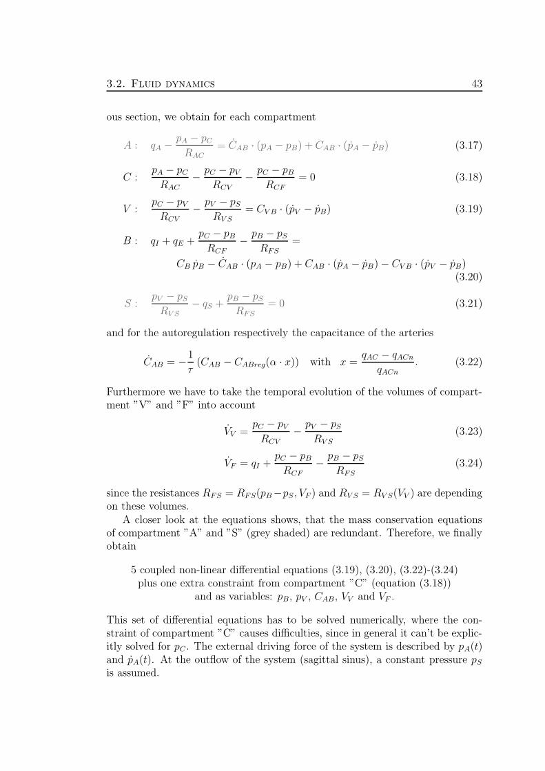
3.2. Fluid dynamics 43
ous section, we obtain for each compartment
A : qA −pA − pC
RAC= CAB · (pA − pB) + CAB · (pA − pB) (3.17)
C :pA − pC
RAC
− pC − pV
RCV
− pC − pB
RCF
= 0 (3.18)
V :pC − pV
RCV− pV − pS
RV S= CV B · (pV − pB) (3.19)
B : qI + qE +pC − pB
RCF− pB − pS
RFS=
CB pB − CAB · (pA − pB) + CAB · (pA − pB)− CV B · (pV − pB)(3.20)
S :pV − pS
RV S− qS +
pB − pS
RFS= 0 (3.21)
and for the autoregulation respectively the capacitance of the arteries
CAB = −1
τ(CAB − CABreg(α · x)) with x =
qAC − qACn
qACn. (3.22)
Furthermore we have to take the temporal evolution of the volumes of compart-ment ”V” and ”F” into account
VV =pC − pV
RCV− pV − pS
RV S(3.23)
VF = qI +pC − pB
RCF− pB − pS
RFS(3.24)
since the resistances RFS = RFS(pB−pS , VF ) and RV S = RV S(VV ) are dependingon these volumes.
A closer look at the equations shows, that the mass conservation equationsof compartment ”A” and ”S” (grey shaded) are redundant. Therefore, we finallyobtain
5 coupled non-linear differential equations (3.19), (3.20), (3.22)-(3.24)plus one extra constraint from compartment ”C” (equation (3.18))
and as variables: pB, pV , CAB , VV and VF .
This set of differential equations has to be solved numerically, where the con-straint of compartment ”C” causes difficulties, since in general it can’t be explic-itly solved for pC . The external driving force of the system is described by pA(t)and pA(t). At the outflow of the system (sagittal sinus), a constant pressure pS
is assumed.

44Chapter 3. Model of the haemodynamic and metabolic processes
in the brain
3.2.4 Standard values
Before verifying the model on data known from medical literature, the standardvalues for the parameters of a healthy patient have to be determined. First thepressure distribution in the cerebral blood vessels will be investigated. This isshown in figure 3.3 for two different medical conditions. The pressure drops fromthe arteries over the capillaries to the veins, where at the end of the veins – inthe sagittal sinus – the pressure is just above 0 mmHg.
As standard values for the pressures in the different compartments we there-fore use
pAn = 100 mmHg pV n = 15 mmHg pBn = pFn = 10 mmHg (3.25)
pCn = 25 mmHg pSn = 5 mmHg. (3.26)
In the medical literature, the standard unit of pressure is mmHg. To make iteasier to compare the results with other works, we also use in this work mmHgas the unit for the pressure.
Figure 3.3: Distribution of the pressure in the blood vessels of the brain(more exactly in the cerebral vascular bed) under normal conditions andin a situation with constricted blood vessels (vasospasm) (adapted fromMchedlishvili [1986]).
For the corresponding volumes, we use the standard values given in the med-ical literature as for example in Purves [1972]
VAn = 15 ml VV n = 40 ml VBn = 1000 ml (3.27)
VCn = 10 ml VSn = 80 ml VFn = 30 ml (3.28)
where for volume VF it has to be noticed, that from medical experiments it isknown that only 30 ml of the total 170 ml cerebrospinal fluid can be absorbed.Most of the CSF is located in the spinal chanal, so that it can not be absorbedin the sagittal sinus.

3.2. Fluid dynamics 45
The main flows of interest are the blood flow from the heart into compartment”A” and the production of cerebrospinal fluid from the capillaries in the ventriclesinto the compartment ”F”, where in medical literature the values
qAn = 600 mlmin
qCFn = 0.4 mlmin
(3.29)
are well established. With these basic parameters the standard values for the re-sistances can be calculated. The resistance between two compartments is definedas the ratio of the pressure difference and the flow between the compartments.For RAC this would be pA−pC
qAn. Taking this into account, we obtain for the blood
and the cerebrospinal fluid circulation (units of resistance is mmHgml/min
):
RACn = 0.125 RV Sn = 0.0166 RCFn = 37.5 (3.30)
RCV n = 0.0166 RFSn = 12.5. (3.31)
Since the resistance RV S is not constant but depending on the volume of com-partment ”V” – see equation (3.15) – we calculate the parameter kRV S
using thevolume VV n to obtain kRV S
= 26.66.To determine the parameter kRAC
in equation (3.8) we first need the capaci-tance of the arteries since the capacitance determines the volume of the compart-ment. Following Ursino and Lodi [1997] the standard value for the capacitanceis
CABn = 0.15 mlmmHg
∆CAB1 = 0.165 mlmmHg
∆CAB2 = 0.065 mlmmHg
(3.32)
while ∆CAB1/2 is determined by the upper (140 mmHg) and lower (70 mmHg)limit of the autoregulation curve. A good review on values of the pressure depen-dence of the autoregulation curve is given in Gao et al. [1998]. The dimensionlessparameter of the strength of the autoregulation can vary from α = 1.5 to α = 0.2for a full functional respectively an impaired autoregulation. The time constantof this process is assumed to be in the range of τ = 10 s (in Giulioni and Ursino[1996] a value of 5 s and in Ursino and Lodi [1997] a value of 20 s is given).
We are using for the capacitances CV B and CB the following parameters asfirst proposed by Ursino [1988] and slightly modified by us for a more realisticbehaviour:
kV = 0.3 1ml
kB = 0.26 1ml
(3.33)
pV 0 = 2.5 mmHg pB0 = 2.5 mmHg. (3.34)
With this set of parameters (valid for a healthy patient) the behaviour of ourmodel can now be validated. After having done this, the same model can thenbe used to reproduce measured data of patients from the intensive care unit.
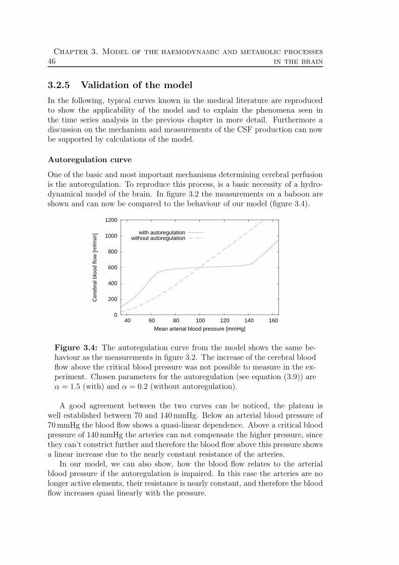
46Chapter 3. Model of the haemodynamic and metabolic processes
in the brain
3.2.5 Validation of the model
In the following, typical curves known in the medical literature are reproducedto show the applicability of the model and to explain the phenomena seen inthe time series analysis in the previous chapter in more detail. Furthermore adiscussion on the mechanism and measurements of the CSF production can nowbe supported by calculations of the model.
Autoregulation curve
One of the basic and most important mechanisms determining cerebral perfusionis the autoregulation. To reproduce this process, is a basic necessity of a hydro-dynamical model of the brain. In figure 3.2 the measurements on a baboon areshown and can now be compared to the behaviour of our model (figure 3.4).
0
200
400
600
800
1000
1200
40 60 80 100 120 140 160
Cer
ebra
l blo
od fl
ow [m
l/min
]
Mean arterial blood pressure [mmHg]
with autoregulationwithout autoregulation
Figure 3.4: The autoregulation curve from the model shows the same be-haviour as the measurements in figure 3.2. The increase of the cerebral bloodflow above the critical blood pressure was not possible to measure in the ex-periment. Chosen parameters for the autoregulation (see equation (3.9)) areα = 1.5 (with) and α = 0.2 (without autoregulation).
A good agreement between the two curves can be noticed, the plateau iswell established between 70 and 140 mmHg. Below an arterial blood pressure of70 mmHg the blood flow shows a quasi-linear dependence. Above a critical bloodpressure of 140 mmHg the arteries can not compensate the higher pressure, sincethey can’t constrict further and therefore the blood flow above this pressure showsa linear increase due to the nearly constant resistance of the arteries.
In our model, we can also show, how the blood flow relates to the arterialblood pressure if the autoregulation is impaired. In this case the arteries are nolonger active elements, their resistance is nearly constant, and therefore the bloodflow increases quasi linearly with the pressure.

3.2. Fluid dynamics 47
Global pressure-volume curve
An important curve showing the behaviour of the system with increase of extravolumes in the brain – for example due to a swelling – is the global pressure-volume curve. In particular the behaviour of the intracranial pressure is of inter-est, since it provides an opportunity to determine the overall compliance of thebrain.
A good review on determining the pressure-volume curve experimentally isgiven in Sklar and Elashvili [1977], where constant flow injection and balloon in-flation measurements are shown. The difference between these two measurementmethods shows up at that point in the curve where the exponential relationshipstarts growing.
In figure 3.5 a balloon inflation measurement is shown. The volume can beincreased by some amount, without any increase of the pressure. This originatesfrom the possibility that some of the CSF is used to compensate this increase ofvolume by absorbing CSF into the blood at the sagittal sinus. Whereas in a flowinjection measurement, the pressure would start growing immediately, since the”effective” volume increase is calculated, where the absorption of the CSF hasalready been taken into account.
In the literature mainly experiments with animals are presented. Data fromhuman patients using the constant flow injection method can be found in Fridenand Ekstedt [1983] as well as similar measurements by Gaab et al. [1983].
Figure 3.5: Global pressure-volume curve/compliance of the brain. Themeasurement of the global compliance is realized by increasing the volume(∆V ) of a balloon in the brain or by injecting and extracting fluid from theCSF compartment. An exponential function can be fitted for the increaseof the intracranial pressure. The resting pressure is then given at ∆V = 0(adapted from Sullivan and Allison [1985]).
As mentioned before, the pressure-volume curve determines the compliancesof the veins and the brain tissue. To check our model, a balloon inflation exper-iment was simulated. The volume of compartment ”E” was steadily increasedand the volume of this compartment was plotted against the intracranial pres-sure, showing the results in figure 3.6. Due to the increase of the compartment

48Chapter 3. Model of the haemodynamic and metabolic processes
in the brain
”E”, in particular the veins and the brain tissue are compressed. The arterialblood vessels have in contrast to that a higher internal blood pressure and activeelements regulating their volume. Therefore their compliance doesn’t play anyrole in the resulting curve.
0
5
10
15
20
25
30
35
40
45
50
0 10 20 30 40 50 0
200
400
600
800
1000
Intr
acra
nial
pre
ssur
e [m
mH
g]
Cer
ebra
l blo
od fl
ow [m
l/min
]
∆V (volume of balloon) [ml]
with autoregulationwithout autoregulation
CBF with autoregulationCBF without autoregulation
VF with and without autoregulation
Figure 3.6: The global pressure-volume curve produced by the model. Theexponential-type increase of the pressure (when the absorbable CSF volumeVF reaches zero) is consistent with figure 3.5. Note, a reduction of the in-crease of the intracranial pressure for impaired autoregulation can be observedaccompanied by a decrease in CBF.
The curve clearly shows that the intracranial pressure only rises when nofurther cerebrospinal fluid can be absorbed (VF ∼ 0). This means that the CSFis used for the compensation of the expanding volume ∆V by absorbing it intothe sagittal sinus.
Furthermore a difference in the increase of the ICP for different states of theautoregulation can be seen. The increase of the ICP is smaller for impaired au-toregulation than for a healthy patient. In this case, the arteries are no longeracting against the external pressure and therefore they will also be compressed.As a result of this, the cerebral blood flow in the impaired autoregulation situ-ation decreases (due to the smaller volume of the arteries and therefore higherresistance) in contrast to a healthy patient.
Cerebrospinal fluid production
From various clinical measurements the production of the cerebrospinal fluidis either assumed to be depending on the cerebral blood flow or to be stableover a wide range of the arterial blood pressure. In Sullivan and Allison [1985]and Hoffmann [1987] these two possibilities are stated. In this section, a short

3.2. Fluid dynamics 49
explanation of the phenomena and the underlying process will be given by usingresults from simulations conducted with the model. The knowledge about theproduction is also important to explain the coupling seen between ABP and ICP.
For our model we used a pure pressure dependent production of the CSF, i.e.the pressure difference between the blood in the capillaries and the pressure ofthe CSF in compartment ”F” is the driving force. Simulations with and withoutworking autoregulation results in the following behaviour for the CBF and CSF-production (figure 3.7).
0
100
200
300
400
500
600
700
800
40 60 80 100 120 140 160 0
0.1
0.2
0.3
0.4
0.5
0.6
0.7
0.8
Cer
ebra
l blo
od fl
ow [m
l/min
]
Cer
ebro
spin
al fl
uid
prod
uctio
n [m
l/min
]
Mean arterial blood pressure [mmHg]
CBF with ARCSF with AR
CBF without ARCSF without AR
Figure 3.7: Dependence of the production of cerebrospinal fluid on thearterial blood pressure. For both states (with and without autoregulation)a good correlation between CBF and CSF-production can be observed, asdocumented by experiments. But the origin of this correlation is the lineardependence of the CSF production on the pressure difference between thecapillary and the CSF compartment!
The plot suggests that the cerebral blood flow is the origin of the CSF produc-tion, since both curves show the same behaviour over the full range of the arterialblood pressure. But effectively a secondary process is seen, the primary processis the pressure depending CSF production. The autoregulation keeps the CBFas well as the pressure in the capillaries constant, therefore the CSF productionis independent of the ABP. But if the autoregulation is impaired the pressure inthe capillaries varies with the ABP, due to the constant resistance of the arteries,and therefore the CSF production grows nearly linearly with the ABP.
Arterial blood pressure - Intracranial pressure
In time series analysis, we have seen a coupling between the arterial blood pres-sure and the intracranial pressure. The question to be asked is, does our model

50Chapter 3. Model of the haemodynamic and metabolic processes
in the brain
reproduce this coupling and if so, under which circumstances? Can we learnanything from the results of such simulations for the treatment of the patients?
We simulated three different situations describing different states of physicalhealth. A patient with...
• active autoregulation and CSF to compensate volume changes (VF > 0)• impaired autoregulation and CSF to compensate volume changes (VF > 0)• impaired autoregulation and no CSF to compensate volume changes (VF = 0)
To visualise a possible coupling, the intracranial pressure is plotted over thearterial blood pressure. The results of the simulations are shown in figure 3.8.
0
5
10
15
20
40 60 80 100 120 140 160
Intr
acra
nial
pre
ssur
e [m
mH
g]
Mean arterial blood pressure [mmHg]
with autoregulation − VF=30mlwithout autoregulation − VF=30mlwithout autoregulation − VF= 0ml
without autoregulation and CB=0 − VF= 0ml
Figure 3.8: Relation between the intracranial pressure (ICP) and the ar-terial blood pressure (ABP) for different states of the autoregulation, thevolume of the CSF fluid (VF ) and the capacitances of the brain tissue (CB).No or only moderate increase of the ICP is seen for situations with fluidin the CSF compartment (VF = 30 ml). For impaired autoregulation andno compensation fluid in the CSF compartment, the increase of the ICPgets stronger especially when the brain tissue is not compressible anymore(CB = 0).
As expected for a healthy patient, the intracranial pressure is independentof the ABP. But if the autoregulation is impaired we obtain a linear increase ofthe ICP. Both phenomena can be explained by the CSF production. As we haveseen in the previous section, the CSF production is depending on the ABP, i.e.for impaired autoregulation a higher CSF production is expected for higher ABP.Due to the constant resistance of the absorption of the CSF, the pressure rises ifmore CSF is produced.
The situation changes clearly if the volume of the cerebrospinal fluid (VF )is fully absorbed, i.e. no compensation fluid is available. This situation was

3.2. Fluid dynamics 51
simulated for blood pressures above 100 mmHg. A sharp bend is seen in thecurves showing a stronger increase of the ICP which can be increased even furtherby assuming the brain tissue to be stiff (CB = 0). The increase is then as strongas the one seen in the time series analysis where the relation between ABP andICP was 3:1 (see figure 2.8).
The main reason for the ICP rising is the increase of the volume of the arteries.Since the autoregulation is impaired, the arteries are passive elements and act likea rubber hose. The volume is then proportional to the ABP. This is equivalentto the phenomenon seen in the global pressure-volume curve. Instead of anexpansion of compartment ”E” – by a swelling or a balloon – the compartment”A” increases its volume due to the impaired autoregulation and results in a riseof the ICP.
Stability analysis of the system of differential equations
To analyse the stability of our system of 5 coupled non-linear differential equa-tions, we calculate the eigenvalues of the Jacobi matrix at their fixed points. Thisgives of course only information about the linear stability as shown in Wiggins[1990]. Interestingly, all fixed points – for physiological reasonable parameters –are stable, i.e. all eigenvalues are negative and real. Furthermore the system hasnot only one fixed point, but a fixed point line. The location of the fixpoints onthis line depends on the initial condition from which the simulation is started.
Oscillating, diverging or chaotic trajectories are not found which seems to betypical for biomedical systems. Still there could be a parameter range – probablyoutside physiologically reasonable parameters – which shows asymptotically nostable solutions.

52Chapter 3. Model of the haemodynamic and metabolic processes
in the brain
3.3 Oxygen transport
As described briefly in the first chapter, the blood circulation is responsible forthe transport of oxygen from the lungs to the cells. As will be seen later, theKrogh cylinder is a good description for the oxygen diffusion processes betweenthe blood in the capillaries and the tissue as well as for the tissue itself. A goodoverview of the oxygen transport in the human body is given in the textbooksby Klinke and Silbernagl [2003] and Greger and Windhorst [1996], as well as inSchmidt et al. [2000].
The intention of this section is the calculation of the mean oxygen pressurein the tissue, which can be measured by a device like the Licox sensor. To beable to do so, all diffusion processes including the cerebral blood flow have to betaken into account. With such a model the relationship between the values ofthe Licox and Invos sensor will be shown. The cerebral blood flow is thereby theorigin of the variations as was seen in time series analysis.
3.3.1 The blood
To supply the cells in the human body with oxygen, the blood first flows throughthe lungs, where due to diffusion processes – triggered by the pressure gradientbetween the oxygen in the air and in the blood – the blood is saturated withoxygen. The oxygen in the blood is mainly bound to the haemoglobin, whichacts as an oxygen buffer. 98% of the oxygen molecules are buffered on the hae-moglobin, only 2% of them are dissolved in the blood. The relation between theoxygen saturated haemoglobin (HbO2) and the dissolved oxygen is described bythe oxygen dissociation curve (ODC), which will be discussed in the followingsection.
Oxygen dissociation curve
The haemoglobin releases the bound oxygen into dissolved oxygen depending onthe oxygen dissociation curve (ODC) as shown in figure 3.9.
From the steep slope between 20 and 50 mmHg of the S-shape curve it can beseen, how the haemoglobin acts as a buffer. Large variations of the saturation ofthe haemoglobin will be reflected only in small variations of the partial oxygenpressure (the dissolved oxygen). Therefore, the dissolved oxygen which is theonly oxygen able for the diffusion into the tissue, is kept stable over a wide range.
First measurements on human blood including a formula for the ODC werepresented by Hill [1910]. Later Adair [1925] proposed a formula with four con-stants reflecting the 4 Fe sites on the haemoglobin to which the O2 molecules canbind. A good explanation for the four constants is given in the book of Crys-tal et al. [1991], where transition probabilities between the states of bound andunbound Fe sites are used.

3.3. Oxygen transport 53
Figure 3.9: Oxygen dissociation curve of human blood. The dissolved oxy-gen respectively the partial pressure of oxygen in the blood (pbO2) is associ-ated with the saturation of haemoglobin with oxygen (HbO2) in an S-shapecurve. Furthermore, the dissociation curve depends on the carbon dioxidecontent (pCO2) in the blood, where pCO2 = 40 mmHg represents normalconditions (adapted from Reneau et al. [1969]).
For our purposes the equation describing the ODC proposed by Hill is suffi-cient, reading
HbO2 saturation = SbO2 =
(p
p50
)n
1 +(
pp50
)n (3.35)
where SbO2 is an abbreviation for the saturation of haemoglobin in the bloodwith O2. p50 defines the oxygen pressure in the blood for a SbO2 of 50%. Typicalvalues for the equation of Hill, using the two constants n and p50, were measuredfor normal conditions by Zwart et al. [1984] (n = 2.5, p50 = 26 mmHg) andSeveringshaus [1979] (n = 2.6, p50 = 27.6 mmHg) as well as derived from theAdair formula with the coefficients given by Roughton and Severinghaus [1973](n = 2.7, p50 = 26.6 mmHg). For our model we will use the following parameters
n = 2.6 and p50 = 26 mmHg. (3.36)
The saturation of haemoglobin with oxygen in the arterial blood is up to 99–100%, i.e. the blood is fully saturated and could only transport more oxygen, ifthe partial pressure of (dissolved) oxygen in the blood is raised. In contrast tothat, the venous blood shows a HbO2 saturation of ”only” 65%, which indicatesstill a good reserve of oxygen.

54Chapter 3. Model of the haemodynamic and metabolic processes
in the brain
Total oxygen content in the blood
First we present a convention for the expressions of the amount of oxygen in theblood. An example would be pbO2, which defines the partial oxygen pressure inthe blood. Now, the first letter can be either
p = pressure [mmHg],
S = saturation of haemoglobin with oxygen [%] or
C = content/amount of oxygen [ cm3 of O2
cm3 of blood]
and the second letter can be either
b = blood, a = arterial or v = venous.
The rest defines the molecule which can be either O2 or CO2. The total amountof oxygen in the blood can be written as a sum of the two terms, the bufferedand the dissolved oxygen
CbO2 = β · SbO2︸ ︷︷ ︸∼ 98%
+ γ · pbO2︸ ︷︷ ︸∼ 2%
(3.37)
where β = 0.201 cm3O2
cm3 and γ = 3 ·10−5 cm3O2
cm3·mmHg, as given in Schmidt et al. [2000]
and other books. CbO2 has therefore the unit cm3 of O2
cm3 of blood. Using normal values
for the saturation and the oxygen pressure, a ratio of 98% of bound oxygen to2% of dissolved oxygen is obtained.
3.3.2 The Krogh cylinder
The oxygen supply of tissue was first described by Krogh [1918-1919] using atissue cylinder around a capillary. In general it is assumed that the oxygen in theblood can reach the tissue only by diffusion. Since the surface to volume ratioin capillaries is the highest, due to their small diameter, here the largest amountof exchange of oxygen takes place. Therefore arteries and veins can be neglectedfor modelling the oxygen transport into the tissue. To get an impression of theKrogh cylinder an illustration is given in figure 3.10.
For simplicity, cylinder coordinates are used in the description of the Kroghcylinder. The z axis lies along the capillary and r defines the radius. At r = rc
the capillary wall touches the tissue cylinder, whereas r = rt defines its overallradius. The length of the tissue cylinder is given by L.
For the description of the Krogh cylinder and the diffusion processes, thefollowing assumptions are made:
i) General: The oxygen pressure gradient as the driving force of the diffusionprocess. In this work, only radial diffusion is taken into account. Calcula-tions of the oxygen pressure in the brain tissue using radial or radial and

3.3. Oxygen transport 55
Figure 3.10: The Krogh cylinder representing a tissue cylinder around acapillary. Red blood cells flow through the capillary carrying the boundoxygen, which, after dissociation into the blood, diffuses into the tissue. rc
defines the capillary radius, rt the radius of the tissue cylinder and ”lethalcorner” the area in the cylinder with the lowest oxygen content (adaptedfrom Reneau et al. [1967]).
axial gradients were performed by Reneau et al. [1967]) and the results areshown in figure 3.11. Only small deviations are seen in the first part of thetissue cylinder. Since we are only interested in the mean oxygen pressurein the tissue cylinder, this deviation cancels out and the axial gradients cantherefore be neglected.
ii) Capillary: The capillaries are straight pipes, running in parallel and hav-ing a unidirectional blood flow. They are arranged in a hexagonal latticeas shown in figure 3.12. The diameter is assumed to be constant and thevelocity profile is uniform, since the red blood cells can only pass the capil-lary one by one as shown in the lower part of figure 3.10. Furthermore theblood flow is assumed to be constant over the whole capillary length. Thecapillary wall represents no resistance to the oxygen diffusion. The oxygenpressure in the capillary is assumed to be constant in r and ϕ.
iii) Tissue: The oxygen consumption in the tissue is assumed to be indepen-dent of the local oxygen pressure (zero-order reaction). The cells may berepresented as a homogeneous volume distribution of sinks of oxygen, in-dependent of time and position. Further the diffusion coefficient can beassumed to be homogeneous.
A way to relax this assumption (which is only necessary for pathologicalcases) is given at the end of this chapter.
Typical values for the radius of the capillary and the tissue cylinder as wellas the length of the cylinder can be found in different books as shown in the
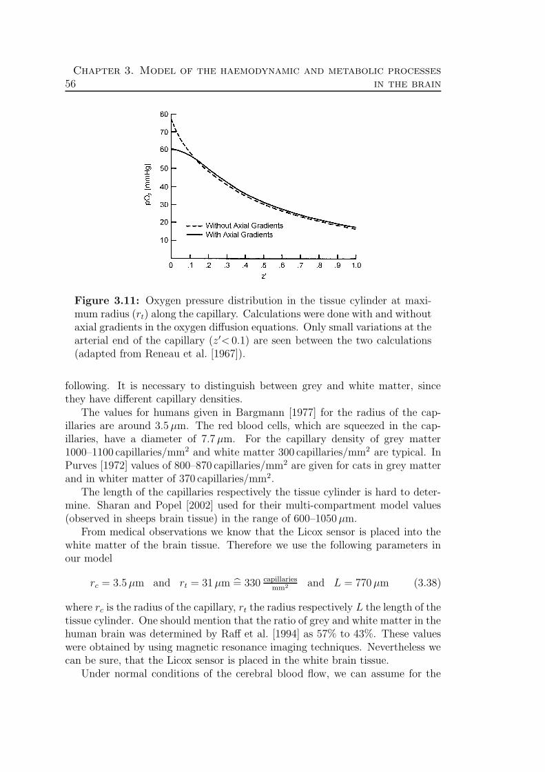
56Chapter 3. Model of the haemodynamic and metabolic processes
in the brain
Figure 3.11: Oxygen pressure distribution in the tissue cylinder at maxi-mum radius (rt) along the capillary. Calculations were done with and withoutaxial gradients in the oxygen diffusion equations. Only small variations at thearterial end of the capillary (z′< 0.1) are seen between the two calculations(adapted from Reneau et al. [1967]).
following. It is necessary to distinguish between grey and white matter, sincethey have different capillary densities.
The values for humans given in Bargmann [1977] for the radius of the cap-illaries are around 3.5 µm. The red blood cells, which are squeezed in the cap-illaries, have a diameter of 7.7 µm. For the capillary density of grey matter1000–1100 capillaries/mm2 and white matter 300 capillaries/mm2 are typical. InPurves [1972] values of 800–870 capillaries/mm2 are given for cats in grey matterand in whiter matter of 370 capillaries/mm2.
The length of the capillaries respectively the tissue cylinder is hard to deter-mine. Sharan and Popel [2002] used for their multi-compartment model values(observed in sheeps brain tissue) in the range of 600–1050 µm.
From medical observations we know that the Licox sensor is placed into thewhite matter of the brain tissue. Therefore we use the following parameters inour model
rc = 3.5 µm and rt = 31 µm = 330 capillariesmm2 and L = 770 µm (3.38)
where rc is the radius of the capillary, rt the radius respectively L the length of thetissue cylinder. One should mention that the ratio of grey and white matter in thehuman brain was determined by Raff et al. [1994] as 57% to 43%. These valueswere obtained by using magnetic resonance imaging techniques. Nevertheless wecan be sure, that the Licox sensor is placed in the white brain tissue.
Under normal conditions of the cerebral blood flow, we can assume for the

3.3. Oxygen transport 57
Figure 3.12: Theoretical arrangement of capillaries in the brain using ahexagonal lattice to guarantee an optimal supply of the tissue with oxygen(adapted from Reneau et al. [1967]).
velocity of the blood respectively the red blood cells typical values of
v = 400 µms
(3.39)
as mentioned in Mintun et al. [2001]. Further, we need for the tissue cylinder theparameters of the consumption, diffusivity and solubility of O2. A good reviewof typical values in oxygen transport in blood and tissue is also given in Mintunet al. [2001], from where we take the following values
A = 4.5 · 10−4 µm3O2
µm3·sand D = 1.8 · 103 µm2
s(3.40a)
and c = 2.6 · 10−5 µm3O2
µm3·mmHg(3.40b)
where A is the O2 consumption, D the O2 diffusivity and c the O2 solubility. InMintun et al. [2001] only a consumption value for grey matter (8.2·10−4 µm3O2
µm3·s) is
given, but from nuclear magnetic resonance imaging measurements in An et al.[2001] the values for grey and white matter were determined as 9.2·10−4 and
4.5·10−4 µm3O2
µm3·s.
58Chapter 3. Model of the haemodynamic and metabolic processes
in the brain
3.3.3 Theory
Our intention is to calculate the mean oxygen pressure in brain tissue (〈ptiO2〉).First of all, we will give a rough outline of the calculation before going into thedetails. The calculations can be divided into two parts, firstly the calculation ofthe oxygen pressure in the blood and secondly the diffusion of oxygen into andwithin the tissue.
The content of oxygen in the blood along the capillary (CbO2(z)) can becalculated by assuming a constant metabolism in the tissue and using the velocityfrom the cerebral blood flow. As boundary condition at the arterial end of thecapillary, the content CbO2(z=0) will be set to the oxygen content of the arterialblood CaO2. For the diffusion processes, the partial pressure of free dissolvedoxygen in the blood (pbO2(z)) is needed. This can be obtained by solving theequation of CbO2(z) for pbO2(z). Unfortunately the pressure can’t be derivedanalytically, therefore either an approximation has to be made (contribution ofpbO2 CbO2) or a nonlinear equation has to be solved numerically.
The oxygen pressure in the tissue will be calculated by using only the radialgradients as mentioned in the assumptions. For the boundary conditions weassume that the pressure is continuous at the interface between capillary andtissue and that the pressure gradient vanishes at the tissue surface (r = rt). Thiscan be satisfied by reasons of symmetry, since the flux through the surface of twoneighbouring tissue cylinders should be zero (flux ∼ pressure gradient – Fick’sfirst law). Therefore we obtain the pressure in the tissue as function of radiusand position along the capillary (ptiO2(r, z)). Finally we have to integrate overthe tissue volume to obtain a value for the mean oxygen pressure in the tissue(as measured by a device like the Licox sensor).
In the following a detailed derivation of the equations will be given.
Oxygen pressure in the blood
From equation (3.37) we obtain the amount of oxygen per blood volume (CbO2).Using the equation of continuity, the CbO2 along the capillary can be calculated.For simplicity we use ρ=CbO2, i.e.
∂ρ
∂t+ divj = α, where j = ρ · v, (3.41)
v is the velocity of the blood in the capillaries (depending on the CBF!) and αdepicts the oxygen consumption from the surrounding tissue. The consumptioncan be calculated from the product of the volume of the tissue cylinder times theoxygen consumption of the tissue
α = −π(rt2 − rc
2)
πrc2
· A (3.42)

3.3. Oxygen transport 59
where A is the constant metabolism of the tissue in units of µm3O2
µm3·s. As a sta-
tionary solution (∂ρ∂t
= 0 and divj = djdz
) and the boundary condition of CaO2 =CbO2(z=0), we obtain
CbO2(z) = CaO2 −rt
2 − rc2
rc2
A
v· z (3.43)
where z is the coordinate along the capillary in units of µm with the arterial endat z = 0. For the diffusion of oxygen into the tissue we need the dissolved oxygen(pbO2) in the blood, which is given implicitly by equation (3.37). The equationconsists of the hill equation plus the linear contribution of the dissolved oxygen
CbO2(z) = β ·(pc(z)
p50
)n
1 +(pc(z)
p50
)n + γ · pc(z) (3.44)
and has to solved for pc(z) – equivalent to pbO2(z) – with the coefficients β =
0.201 cm3O2
cm3 and γ = 3 · 10−5 cm3O2
cm3·mmHg. We obtain as solution an equation of the
form
γ
p50n· pn+1
c (z)− CbO2(z)− β
p50n
· pnc (z) + γ · pc(z)− CbO2(z) = 0 (3.45)
where CbO2(z) has to be replaced by equation (3.43). The solution for pc(z) ofthis equation will give the correct oxygen pressure in the blood (pbO2(z)), butunfortunately there is no general analytic solution for arbitrary n – not even forn = 3.
Two possibilities exist to obtain a value for the pressure of the dissolvedoxygen in the blood (pbO2(z)): Either we solve the equation numerically, butthis will lead to a stepwise numerical integration of the final integral for themean oxygen pressure in the tissue or we use an approximation ignoring the lastpart of equation (3.44), since for normal physiological conditions the contributionis only 2%, leading to an analytical solution. Using the approximation, we thenonly have to deal with the saturation of the haemoglobin (SbO2) and not withthe full oxygen content of the blood (CbO2). This simplifies the calculation to
SbO2(z) =
(pc(z)p50
)n
1 +(pc(z)
p50
)n solved for pc: pc(z) = p50 ·(
SbO2(z)
1− SbO2(z)
) 1n
(3.46)
with SbO2 depending on the position z along the capillary
SbO2(z) = SaO2 −rt
2 − rc2
rc2
A
v· z (3.47)
which is similar to equation (3.43).

60Chapter 3. Model of the haemodynamic and metabolic processes
in the brain
Oxygen diffusion in the tissue
Calculating the diffusion from the capillary wall into and within the tissue we useFick’s second law. The derivation is based on definition of the flux as j = −D∇pfrom the oxygen pressure field and applying the mass conservation, i.e. the massbalance for diffusive O2 transport and O2 consumption: ∇ · j + α = 0. For thetime depending equation, we write
∂p
∂t= D ·∆p− A
c(3.48)
with A the metabolism of the tissue, c the oxygen solubility coefficient and Dthe oxygen diffusivity in the tissue. Due to the geometry of the model, we usecylindrical coordinates. Since we know that we can ignore axial diffusion, i.e.along the z coordinate, and can assume the tissue to be homogeneous, i.e. nogradients depending on ϕ, we write Fick’s second law as
∂p
∂t= D ·
(∂2p
∂r2+
1
r
∂p
∂r
)− A
c. (3.49)
To solve this equation, we use the following boundary conditions as they werementioned in the introduction
p = pc at r = rc and∂p
∂r= 0 at r = rt (3.50)
where pc is the oxygen pressure in the capillary obtained either from equa-tion (3.45) or (3.46). Assuming further a steady state, we obtain the solutionfor the oxygen pressure in the tissue
pti(r, z) = pc(z)− A
2Dc
(rt
2 lnr
rc+
1
2(rc
2 − r2)
)(3.51)
as was already shown in Krogh [1918-1919], where a Danish friend of him, themathematician Mr-. K. Erlang, derived this solution. Finally, to calculate themean partial pressure of oxygen in the tissue we have to integrate over the tissuecylinder
pti = 〈pti(r, z)〉Vtissue=
1
Vtissue
∫ L
0
∫ 2π
0
∫ rt
rc
pti(r, z) · r dr dϕ dz (3.52)
with Vtissue = π(rt2−rc
2)L. This is the general form of the mean oxygen pressurein the tissue. Note, our expression of pti(r, z) is only valid if the pressure ispositive at any point in the tissue cylinder. For normal physiological conditions,as we will assume for the following calculations, a positive pressure in the tissuecan be assumed. Therefore the constant extraction of O2 (independent of z), as

3.3. Oxygen transport 61
given in equation (3.42), is still valid. The integral can then be solved partiallyand the mean oxygen pressure in the tissue can be written as
pti =1
L
∫ L
0
pc(z) dz − A
8Dc·−rc
4 + 4rc2rt
2 − 3rt4 + 4rt
4ln rt
rc
rt2 − rc
2. (3.53)
But the integral over pc(z) has still to be solved separately. Either we use equa-tion (3.45), but then the nonlinear equation has to be solved in every integrationstep, or we use the approximation (ignoring the dissolved oxygen in the calcu-lation of the total amount of oxygen in the blood) given in equation (3.46) and(3.47). Using this approximation, we then obtain
pti =p50
L
∫ L
0
(a− bz
1− (a− bz)
) 1n
dz − A
8Dc·−rc
4 + 4rc2rt
2 − 3rt4 + 4rt
4ln rt
rc
rt2 − rc
2
(3.54a)
where a = SaO2 and b =rt
2 − rc2
rc2
A
v. (3.54b)
The integral has unfortunately no closed solution for arbitrary n, but a solutioninvolving hypergeometric functions can be given and solved numerically.

62Chapter 3. Model of the haemodynamic and metabolic processes
in the brain
3.4 Validation: Theory ↔ Experimental data
In the following a validation of the theoretical description of the oxygen diffusionprocesses in the human brain as well as a validation of the combined hydrody-namical and oxygen supply model will be given. We will compare the theoreticalprediction from the model with the experimentally measured data from patientsat the intensive care unit. Finally we will address the problem of the to highabsolute values of the theoretical predictions and give a suggestion for a solution.
Oxygen supply model: Licox ↔ Invos
In the time series analysis chapter, the question of the functional relationshipbetween the measured values of the Licox and Invos sensors was raised. Withthe here presented theoretical framework we are able to give an answer to thisquestion and to proof the validity of it by a comparison of the predictions withthe measured data.
A plot showing the relationship between the pressure of oxygen in the tissue(Licox) and the saturation of haemoglobin with oxygen (Invos) is given in fig-ure 3.13. Due to the long term trends in the data sets, only the variations areshown to enable a comparison with the theoretical predictions. From a 48 hoursrecording, only those time sections where no external influence on the patienttook place, were used. This resulted in 30 hours of undisturbed data.
From the medical point of view, the variations in the measured values of bothsensors are mainly due to the changes of the cerebral blood flow. To be ableto compare the theoretical predictions with the measured data, we calculate thetheoretical values for Licox and Invos for varying cerebral blood flow using equa-tion (3.53). Thereby the velocity in the capillaries is assumed to be proportionalto the cerebral blood flow. The variable used for the theoretical Licox value is pti,whereas for the Invos sensor a ratio of 1:3 of the arterial and venous saturatedblood (SaO2 and SvO2) is used as was stated in equation (1.3). Overlaying themeasured data with the theoretical curve results in the plot shown in figure 3.13.
At first sight, the relation between Licox and Invos obtained from the theo-retical calculation shows a nearly linear correlation for the variation of the bloodvelocity. The measured signals are not exactly following the theoretical descrip-tion – which was expected for the description of such a complex system – but themain behaviour is well described. One should propably notice, that the resolu-tion of the Invos sensors is given as ±1%. Therefore only for the larger variations(where the influence of the measurement inaccuracy is small) it can be expectedthat the measured data follows the theoretical predictions. The linear behaviourof the prediction explains now, why a good correlation was seen between the twosensor signals in the (linear) time series analysis.
Before taking the rest of the 48 hours time series into account, we shouldmention the air tube cleaning manoeuvre performed by nurses on the patient.

3.4. Validation: Theory ↔ Experimental data 63
−4 −2 0 2 4 6
−4
−2
0
2
4
6 ∆v=25 m/sµ
v=400 m/sµ
∆ H
bO2 [%
]
∆ ptiO
2 [mmHg]
Figure 3.13: Relation between Licox (ptiO2) and Invos (HbO2). Shown isthe data from a patients recording (red dots) compared to the theoreticalprediction (green line). The variations are assumed to depend on the vari-ability of the cerebral blood flow respectively the velocity of the blood in thecapillaries. Note: The plotted data originates from times with no externalinfluence on the patient (30 h of 48 h recording).
Due to the artificial ventilation of the patients, the air tube fills itself with amucus (a slime) leading to a smaller tube radius. The tube has therefore to becleaned regularly. During the cleaning, the patient has no artificial ventilation,which could lead to an oxygen undersupply. To overcome this problem, thepatient is supplied (a few minutes before the manoeuvre) with air containing100% oxygen.
In figure 3.14 the remaining 18 hours of the data are plotted as grey dots,while still showing the 30 hours data (red dots) from the previous figure 3.13.The blue line is a theoretically calculated curve based on the variation of thearterial oxygen pressure paO2. The velocity of the blood was kept constant at400 µm/s. The paO2 values – corresponding to the circles on the line – areincreased quadratically from 50 mmHg to 700 mmHg.
We can clearly see a strong increase of ptiO2 when paO2 is increased above100 mmHg. In contrast to the ptiO2 value, the HbO2 value saturates slowly.This can be described by the higher dissolved oxygen content in the blood. Thehaemoglobin saturation is not strongly increased by the higher paO2 (due to thenonlinearity of the ODC), but more dissolved oxygen is available for diffusion intothe tissue. This results automatically in a higher oxygen content in the tissue andtherefore higher values from the Licox sensor. The behaviour of the curves shownby the grey dots – mostly originating from the air tube cleaning manoeuvre – arethus described and understood using the variation of the arterial oxygen pressure.
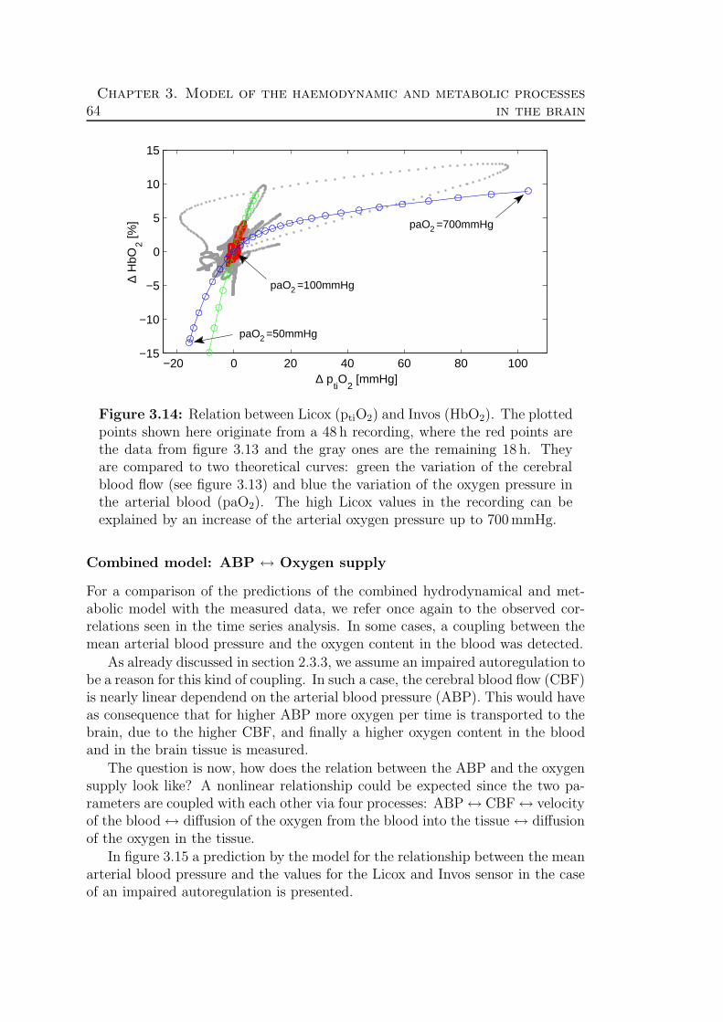
64Chapter 3. Model of the haemodynamic and metabolic processes
in the brain
−20 0 20 40 60 80 100−15
−10
−5
0
5
10
15
paO =100mmHg2
paO =700mmHg2
paO =50mmHg2
∆ H
bO2 [%
]
∆ ptiO
2 [mmHg]
Figure 3.14: Relation between Licox (ptiO2) and Invos (HbO2). The plottedpoints shown here originate from a 48 h recording, where the red points arethe data from figure 3.13 and the gray ones are the remaining 18 h. Theyare compared to two theoretical curves: green the variation of the cerebralblood flow (see figure 3.13) and blue the variation of the oxygen pressure inthe arterial blood (paO2). The high Licox values in the recording can beexplained by an increase of the arterial oxygen pressure up to 700 mmHg.
Combined model: ABP ↔ Oxygen supply
For a comparison of the predictions of the combined hydrodynamical and met-abolic model with the measured data, we refer once again to the observed cor-relations seen in the time series analysis. In some cases, a coupling between themean arterial blood pressure and the oxygen content in the blood was detected.
As already discussed in section 2.3.3, we assume an impaired autoregulation tobe a reason for this kind of coupling. In such a case, the cerebral blood flow (CBF)is nearly linear dependend on the arterial blood pressure (ABP). This would haveas consequence that for higher ABP more oxygen per time is transported to thebrain, due to the higher CBF, and finally a higher oxygen content in the bloodand in the brain tissue is measured.
The question is now, how does the relation between the ABP and the oxygensupply look like? A nonlinear relationship could be expected since the two pa-rameters are coupled with each other via four processes: ABP↔ CBF↔ velocityof the blood↔ diffusion of the oxygen from the blood into the tissue ↔ diffusionof the oxygen in the tissue.
In figure 3.15 a prediction by the model for the relationship between the meanarterial blood pressure and the values for the Licox and Invos sensor in the caseof an impaired autoregulation is presented.

3.4. Validation: Theory ↔ Experimental data 65
20
25
30
35
40
45
50
55
60
60 80 100 120 140 160 20
30
40
50
60
70
80
90
100
p tiO
2 [m
mH
g]
HbO
2 [%
]
Mean arterial blood pressure [mmHg]
Licox ( )ptiO2
Invos ( )HbO2
Figure 3.15: Predictions from the combined model for the relation betweenthe mean ABP and Licox (ptiO2) respectively Invos (HbO2) in the case ofan impaired autoregulation. A nonlinear relationship is observed for bothsensors. But in the typical ABP range of 80 to 110 mmHg, in particular theLicox values correlates nearly linear with the ABP.
In this figure, two interesting observations can be made. First the globalbehaviour of both values (ptiO2 and HbO2) over the full range of the mean arterialblood pressure shows a nonlinear relationship. In particular the predicted valuesfor the Invos sensor show a steep slope for low ABP values and a strong saturationfor high ABP values. But in the typically observed ABP range of 80 to 110 mmHg,both predicted curves can be well approximated by a linear relationship. Inparticular the Licox values follow nicely a straight line.
This linear relationship explains now the well established linear correlationfound in time series analysis, making us confident that the combined model de-scribes both metabolic and hydrodynamical processes correctly. To support thisclaim, we will compare the 21 hours recording used for the correlation analysisin figure 2.7 with the theoretical predictions. In figure 3.16 the variations of therecorded Licox values are plotted versus the mean arterial blood pressure (reddots), after removing trends and noise from the data as described in chapter 2.2.Further the theoretical prediction from the model for the case of an impairedautoregulation is shown (green line).
During this 21 hours recording, the patient is assumed to be in the same stateof health, in particular having an impaired autoregulation. Of course externalinfluences to the patient will be reflected in the data. Nevertheless the measureddata follows mainly the prediction, even when sometimes larger deviations areseen. Furthermore inaccuracies from the Licox sensor or a wrong drift removalinduce large deviations.
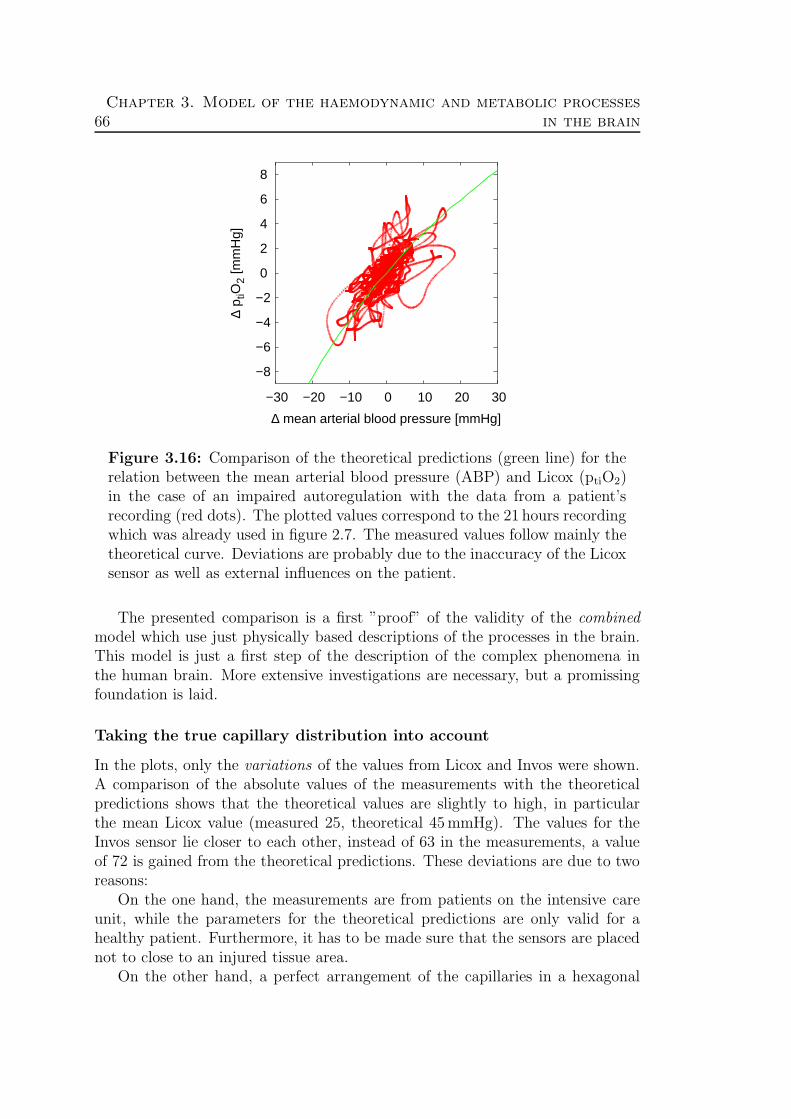
66Chapter 3. Model of the haemodynamic and metabolic processes
in the brain
−8
−6
−4
−2
0
2
4
6
8
−30 −20 −10 0 10 20 30
∆ p t
iO2
[mm
Hg]
∆ mean arterial blood pressure [mmHg]
Figure 3.16: Comparison of the theoretical predictions (green line) for therelation between the mean arterial blood pressure (ABP) and Licox (ptiO2)in the case of an impaired autoregulation with the data from a patient’srecording (red dots). The plotted values correspond to the 21 hours recordingwhich was already used in figure 2.7. The measured values follow mainly thetheoretical curve. Deviations are probably due to the inaccuracy of the Licoxsensor as well as external influences on the patient.
The presented comparison is a first ”proof” of the validity of the combinedmodel which use just physically based descriptions of the processes in the brain.This model is just a first step of the description of the complex phenomena inthe human brain. More extensive investigations are necessary, but a promissingfoundation is laid.
Taking the true capillary distribution into account
In the plots, only the variations of the values from Licox and Invos were shown.A comparison of the absolute values of the measurements with the theoreticalpredictions shows that the theoretical values are slightly to high, in particularthe mean Licox value (measured 25, theoretical 45 mmHg). The values for theInvos sensor lie closer to each other, instead of 63 in the measurements, a valueof 72 is gained from the theoretical predictions. These deviations are due to tworeasons:
On the one hand, the measurements are from patients on the intensive careunit, while the parameters for the theoretical predictions are only valid for ahealthy patient. Furthermore, it has to be made sure that the sensors are placednot to close to an injured tissue area.
On the other hand, a perfect arrangement of the capillaries in a hexagonal

3.4. Validation: Theory ↔ Experimental data 67
lattice is assumed. This is of course not true for natural systems. The distancedistribution of the nearest neighbours will be widely spread and we don’t have(as assumed here) a delta peak at fixed rt. In the book of Hoofd [1992] it wasshown – using a large lattice on which the diffusion equation was solved – that arandomly distributed arrangement of capillaries shows a decrease of the oxygenpressures in the tissue. Since in the equations given in this work, the radius ofthe tissue cylinder rt can be varied, the overall mean oxygen pressure for truenatural systems can be calculated by integrating over all possible tissue radii
〈pti(rt)〉all possible tissue radii =
∫ ∞
0
ϕ(r) · pti(rt = r) · r2 · L dr (3.55)
where ϕ(r) is the probability to find the nearest neighbour capillary at distancer.
Note: Attention should be paid to the fact that the oxygen pressure in thetissue (pti(r, z)) can get negative for large tissue cylinders rt. A negative partialoxygen pressure is of course non-physical and therefore the formulas/boundaryconditions have to be adapted. This can be done by choosing the tissue radius rt
in equation (3.50) so that it fulfils the conditions
pti = 0 and∂p
∂r= 0 at r = r∗t (3.56)
as it was mentioned briefly in Reneau et al. [1970]. If the radius of the tissuecylinder rt is larger than r∗t , the oxygen pressure in the tissue (pti) is zero, i.e.pti(r > r∗t ) = 0.
The two boundary conditions are getting clear when we think about, whichconditions must be fulfilled at the point, where the oxygen pressure reaches zero.Since the oxygen pressure reaches zero (pti = 0 at r = r∗t ), the flux throughoutthis point is zero (no oxygen molecules will diffuse through out this point). Butthis is equivalent to a vanishing pressure gradient ( ∂p
∂r= 0 at r = r∗t ).
First preliminary tests showed, that the calculation with this modification tothe formulas results in a much better agreement with the measured values. Theoverall mean oxygen pressure in the tissue reaches now values of 30 mmHg insteadof 45 mmHg in the previous calculations.

68Chapter 3. Model of the haemodynamic and metabolic processes
in the brain
3.5 Conclusions
In this chapter we have shown that mathematical models of the haemodynamicand metabolic processes are useful for a deeper understanding of complex pro-cesses occurring in the human brain in normal and pathophysiological states.
A hydrodynamical compartment model was established by a pure physical de-scription and adapted to the special requirements of the neurosurgical intensivemedicine. The special properties of the individual compartments, as for examplethe autoregulation, the cerebrospinal fluid (CSF) production and the compres-sion of the veins, were described. From the equation of continuity, a system of 5coupled nonlinear differential equations plus one constrain was derived. We wereable to reproduce the important interdependencies known from medical literatureas for example the autoregulation or the pressure-volume curve. Furthermore,the observation of the (indirect) cerebral blood flow dependent production of theCSF could be explained, by showing that the observations are only secondaryprocesses. The primary (underlying) processes is the pressure depending pro-duction of the CSF. Finally, the main advantage of this model is the possibilityto estimate the cerebral blood flow continuously in contrast to already existingimaging techniques.
Further, an oxygen supply model was derived using the theory of the Kroghcylinder. With this relatively simple model consisting of a capillary surroundedby a tissue cylinder, we are able to describe the oxygen supply processes in thebrain. As the basic mechanism, a pressure gradient driven diffusion was usedto determine the oxygen content in brain matter. Interestingly, the theoreticalpredictions for the values of Licox and Invos show a nearly linear correlation forvarying blood velocity. The nonlinear oxygen diffusion curve as well as the diffu-sion processes only play a role, when huge changes to the physiological conditionstakes place, as for example in the air tube cleaning manoeuvre. We could showhow these large oscillations in the Licox measurements could be described by avariation of the partial oxygen pressure in the arterial blood.
Finally both models were combined to simulate the measurements obtainedby recordings from the intensive care unit. Thereby, the cerebral blood flowestimated by the hydrodynamical model acts as the link to the oxygen supplymodel. By means of the combined model the results of the correlation analysiscould be confirmed and the measurements quantitatively be reproduced. There-fore, a better insight into the underlying processes generating these correlationswas achieved by this model.

Chapter 4
Independent component analysis
Independent component analysis (ICA) is a multimodal time series analysis tech-nique to find statistical independent signals within a given data set.
A typical example for the application of ICA is the cocktail party problem,a so-called blind source separation (BSS) problem. Imagine a group of n peoplestanding around chatting with each other. This mixture of signals is recordedby n microphones. The goal is to extract from the mixture of speech signals thevoices of the speakers (the sources) without knowing the sources and the mixtureprocess (therefore called blind). Assuming the voices to be independent – whichis a valid assumption – the method of ICA can be applied and a correspondingalgorithm is then able to recover, just by using the mixed signals, the voice ofeach speaker.
ICA seems not only to be able to find the correct solution in the cocktailparty problem, but also to reveal the essential structures of the data in many(real world) applications. The assumption of the independence of the signalsappears to be a very strong property and in particular useful when applying itto the analysis of highly multimodal data sets.
In this chapter the derivation of two new algorithms using a geometric ap-proach and an information theoretical one including time structures is presented.Furthermore the application to biomedical data sets – in particular to EEG data –is shown while the limitations of the method are also discussed.
4.1 Introduction
Independent component analysis is a signal processing tool to decompose observedsignals x(t) ∈ R
m into a set of statistically independent signals y(t) ∈ Rm, which
are called the independent components. Statistical independence has to be seenin the mathematical sense of stochastically/statistically independent probability
69

70 Chapter 4. Independent component analysis
densities, i.e. the joint probability density factorises into the marginal densities
p(y) =n∏
i=1
p(yi) (4.1)
where y is an n-dimensional random variable with yi its ith component. The ideaof decomposing signals into independent signals was first expressed by Jutten andHerault [1991] in the framework of blind separation of sources, while the term”ICA” was later coined by Comon [1994] in his fundamental paper on the theoryof linear ICA.
However the field became quickly popular with the seminal paper by Bell andSejnowski [1995] who elaborated upon the Infomax-principle, first introduced byLinsker [1992]. Later Amari [1998] introduced the concept of a natural gradientsimplifying the Infomax learning rule. Among others, the most efficient ICA al-gorithm developed in the following year was the FastICA-algorithm by Hyvarinen[1999] using negentropy and kurtosis as a contrast function. Recently, geomet-ric ICA algorithms first proposed by Puntonet et al. [1995], which are based onneural learning clustering algorithms, have received further attention due to theirrelative ease of implementation.
For a good introduction to ICA together with extensions to various cases andapplications of ICA we refer to one of the following text-books: Hyvarinen et al.[2001], Cichocki and Amari [2002] and Lee [1998].
The blind source separation problem
The most prominent application of ICA is the blind source separation problem.There an underlying mixture model generates the observed signals x(t) from thesources s(t) by x(t) = f(s(t)), where f(·) can be a (non-)linear function mappingfrom R
n → Rm. For the linear case, which is commonly investigated and on
which will be focused in this work, the observed signals are generated by
x(t) = A · s(t) (4.2)
where s(t) are the n-dimensional independent sources, x(t) depicts the m dimen-sional mixed/measured signals and A is the m×n mixing matrix. The goal of theBSS problem is to find the unknown sources s(t) and the unknown transformationmatrix A.
An ICA algorithm is trying to find as independent signals as possible fromthe mixture of signals x(t) by using – in the linear case – an unmixing matrix W,so that the independent components can be written as y(t) = W · x(t). Oftenonly the quadratic case is investigated, where the number of sources equals thenumber of observation (m = n).
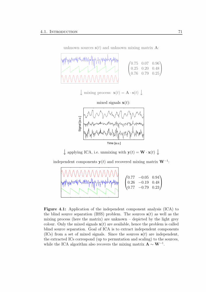
4.1. Introduction 71
unknown sources s(t) and unknown mixing matrix A:
0.75 0.07 0.960.25 0.20 0.480.76 0.79 0.25
↓ mixing process: x(t) = A · s(t) ↓mixed signals x(t):
Sig
nal [
a.u.
]
Time [a.u.]
↓ applying ICA, i.e. unmixing with y(t) = W · x(t) ↓independent components y(t) and recovered mixing matrix W−1:
0.77 −0.05 0.940.26 −0.19 0.480.77 −0.79 0.23
Figure 4.1: Application of the independent component analysis (ICA) tothe blind source separation (BSS) problem. The sources s(t) as well as themixing process (here the matrix) are unknown – depicted by the light greycolour. Only the mixed signals x(t) are available, hence the problem is calledblind source separation. Goal of ICA is to extract independent components(ICs) from a set of mixed signals. Since the sources s(t) are independent,the extracted ICs correspond (up to permutation and scaling) to the sources,while the ICA algorithm also recovers the mixing matrix A ∼W−1.

72 Chapter 4. Independent component analysis
The reason for the restriction to the quadratic case is that it can be proofen(as done by Comon [1994]) that the assumption of independent sources is strongenough to solve the (quadratic) BSS problem correctly up to an indeterminacyof scaling and permutation of the recovered sources. A further restriction, whichwill get obvious in the following theory section, is that maximally one source mayhave a probability function equal to a gaussian density. Typically this proof fromComon is called the proof of the identifiability of quadratic linear ICA.
For BSS problems with more signals than sources (m > n), the problem caneasily be reduced by a principal component analysis to the quadratic case, sinceno additional information is gained by further linear combinations of the sourcesas shown in great detail in the book of Hyvarinen et al. [2001]. In contrast tothat, the BSS problem with more sources than measured signals (n > m) has– without any additional knowledge – no unique solutions and is referred to asovercomplete ICA, since the basis (the sources) represents an overcomplete basisfor the measured signals. First approaches to algorithms solving overcompleteICA problems were presented by Lewicki and Sejnowski [1998]. Later Theis et al.[2003a] presented a procedure using geometric considerations.
In the quadratic case, the recovered mixing matrix W−1 is said to be similarto A, when the recovered sources differ to the original sources only by scalingand permutation. The unmixed signals respectively the independent componentscan then be written as
y(t) = W · x(t)
= W ·A · s(t)= S ·P · s(t)
(4.3)
where S is a scaling matrix with coefficients only on the diagonal and P is thepermutation matrix. Both matrices are for the quadratic case of the size n× n.For an illustration of the application of ICA to a BSS problem see figure 4.1.
ICA can be applied in many other areas. The cocktail party problem is a niceand intuitive example, which shows the basics of speech processing. Beside thismore artificial application, the method is also of great interest for remote sensing,image recovery and biomedical applications. In this chapter, we will show howthe ICA method can be applied to biomedical data sets and where the limitationsof this method are.
Before presenting the applications, a short introductory section will make thereader familiar with the notation and the basic concepts used in probability andinformation theory. Subsequently, two new algorithms are derived using two verydifferent approaches. Firstly a geometrically supported algorithm using scatterplots and their properties under transformation and secondly an approach usinginformation theory including the knowledge of time structures in the data, as itis used in the framework of time series analysis.

4.2. Basic theory 73
4.2 Basic theory
In this section a short review on the basic probability- and information-theoreticaldefinitions is given to make the reader familiar with the notation used in this work.The introduction follows mainly the theory chapters of Hyvarinen et al. [2001]using the same notation.
4.2.1 Probability theory
For a more detailed introduction to probability theory the book by Papoulis[1991] is recommended, which includes also the proofs of statements given inthese sections.
Random variables and probability distributions
In this work we are assuming random variables as continuously-valued unlessstated otherwise. The cumulative distribution function (cdf) Fx of a randomvariable at point x = x0 is defined as the probability that x ≤ x0
Fx(x0) = P (x ≤ x0) (4.4)
where x0 can take values between −∞ to ∞, defining the whole cumulativedistribution function for all values of x. The cdf for continuous random variablesis a nonnegative, nondecreasing continuous function whose values lie in the range0 ≤ Fx(x) ≤ 1. From equation (4.4) it follows directly that Fx(−∞) = 0 andFx(+∞) = 1.
The probability density function (pdf) of a random variable x can then bedefined as the derivative of its cumulative distribution function
px(x0) =dFx(x)
dx
∣∣∣∣x=x0
. (4.5)
The normalisation of the probability density function follows directly from thedefinition of the cdf ∫ +∞
−∞
px(x) dx = 1. (4.6)
The concept of probability distributions can easily be generalised to randomvectors. Assuming that x is an n-dimensional random vector x = (x1, x2, ..., xn)T ,where the components x1, x2, ..., xn are continuous random variables. T denotesthe transpose of the vector. We will deal in this work only with column vectorsunless stated otherwise. The same definition for the cdf and pdf can be formulatedfor random vectors as shown in Papoulis [1991] and Hyvarinen et al. [2001].
A special set of probability densities are the conditional densities. They arenecessary to answer the question: ”What is the probability density of a ran-dom vector x given another random vector y?” Assuming that the joint density

74 Chapter 4. Independent component analysis
px,y(x,y) of x and y and the (marginal) density py(y) exist, the conditionalprobability density of x given y is defined as
px|y(x|y) =px,y(x,y)
py(y). (4.7)
Expectations and moments
Often the expectations of some functions of a random variable are of interest forthe analysis and the processing of data. A great advantage of expectations isthe possibility to directly derive them from the data, although they are formallydefined in terms of the probability density function.
Let g(x) be any quantity of the random variable, which can be either a scalar,a vector or a matrix. The expectation of g(x) is denoted by Eg(x) and is definedas
Eg(x) =
∫ +∞
−∞
g(x) px(x) dx. (4.8)
The integration operation is applied separately to every component of the vectoror every element of the matrix resulting in another vector or matrix of the samesize.
Usually the probability density of a random vector is unknown, but often aset of N samples x1,x2, ...,xN from x is available, as for example in the case ofdata measured in real world applications. The expectation can then be estimatedby averaging over the samples using
Eg(x) ' 1
N
N∑
i=1
g(xi). (4.9)
If g(x) is of the form xn, i.e. products of the random variable, we end up at thenth moment, denoted by αn and defined by
αn = Exn =
∫ +∞
−∞
xn px(x) dx. (4.10)
Often the central moments µn are more useful, which are computed around themean (mx= α1 = 1st moment) of x
µn = E(x−mx)n =
∫ +∞
−∞
(x−mx)n px(x) dx. (4.11)
From the definition it follows directly that the central moments µ0 = 1, due tonormalisation, and µ1 = 0, due to the removal of the mean, are insignificant.

4.2. Basic theory 75
But the higher central moments, used in the so-called higher order statistics, cancontain valuable information. In the literature the following variables are defined
σ2 = µ2 the variance of x, (4.12)
γ =µ3
σ3the skewness of x, (4.13)
κ =µ4
σ4− 3 the kurtosis of x. (4.14)
In words, the variance gives an estimate of the width of the distribution, theskewness of the asymmetry of the distribution and the kurtosis an estimate ofthe deviation from a gaussian distribution. As we will see later, the gaussiandistribution has very special properties, its kurtosis is zero and due to its sym-metry it has also zero skewness. Therefore it is often used as a reference. In onedimension one can write
px(x) =1√2π σ
· e− x2
2σ2 . (4.15)
Correlation and independence
The correlation between ith and jth component of a random vector x is denotedby rij and given by
rij = Exixj =
∫ +∞
−∞
∫ +∞
−∞
xi xj pxi,xj(xi, xj) dxj dxi (4.16)
where the correlation can be positive or negative. Is the correlation equal to zero,we speak of uncorrelated random variables. For the calculation of all correlationsbetween the components of the random vector x we can write a n × n matrix,the correlation matrix
Rx = ExxT. (4.17)
Using the central moments we can also define a sort of correlation matrix, theso-called covariance matrix, where the mean of the random vector is removedprior to the calculation
Cx = E(x−mx)(x−mx)T. (4.18)
If the mean mx is zero, the correlation and covariance matrices become equal.The expectation operation can be extended to functions g(x,y) of two differentrandom vectors x and y in terms of their joint probability density
Eg(x,y) =
∫ +∞
−∞
∫ +∞
−∞
g(x,y) px,y(x,y) dy dx (4.19)
76 Chapter 4. Independent component analysis
where the integrals are computed over all components of the random vectors. Inanalogy to the correlation and covariance matrix definitions, we can define theso-called cross-correlation and cross-variance matrix of x and y as
Rxy = ExyT and Cxy = E(x−mx)(y−my)T. (4.20)
Two random vectors x and y are called uncorrelated if their cross-covariancematrix Cxy is a zero matrix Cxy = 0.
The mathematical definition of independence of two random variable x andy (as it is used in ICA) is defined by the factorisation of the joint probabilitydistribution px,y(x, y) into the product of their marginal densities px(x) and py(y),i.e. we write
px,y(x, y) = px(x) · py(y). (4.21)
More general the components of a random vector x are independent, if
p(x) =n∏
i=1
p(xi). (4.22)
It follows directly from this definition that independent variables satisfy the basicproperty
Eg(x)h(y) = Eg(x) · Eh(y) (4.23)
where g(x) and h(y) are any absolutely integrable functions of x and y, respec-tively. This reveals that statistical independence is a much stronger propertythan assuming uncorrelated variables. For uncorrelated variables, g(x) and h(y)are just linear functions, taking only the so-called second-order statistics intoaccount.
However, if the random variables have gaussian distributions and are uncorre-lated, then they are also independent. This is a very special property of gaussiandistributions. It gets obvious when we write down the n-dimensional probabilitydensity of a gaussian random vector x
px(x) =1
(2π)n/2√
detCx
· e− 12(x−mx)T C−1
x(x−mx). (4.24)
Assuming that x is uncorrelated, it follows directly that Cx is a diagonal matrixand further the inverse C−1
x is of a diagonal form. This results in a sum in theexponent with which the probability density px(x) factorises. But the factorisa-tion is the criterion of independence. Therefore uncorrelated gaussian randomvectors are independent.
Furthermore it becomes obvious, why independent component analysis cannot find the correct (de)mixing matrix, if more than one source is gaussian dis-tributed. Assume x is an independent gaussian distributed random vector withzero mean (mx = 0) and its probability density equals equations (4.24). Then,

4.2. Basic theory 77
under every transformation of an orthogonal matrix O so that y = Ox, theprobability density of y does not change. Using the property OT = O−1 ofthe orthogonal matrix shows directly the equality of the probability densities(p(y) = p(x)). Therefore ICA can only find the (de)mixing matrix of a mixtureof gaussian distributed random variables up to an orthogonal matrix.
Markov chains
A class of random processes that is rich enough to capture a large variety oftemporal dependencies is the class of finite state Markov processes. In the Markovchain model, the current state of the process depends on a certain number ofprevious values of the process. The number depicts the order of the process.
Such a process is characterised by its order m, and by a conditional probabilitymatrix Pm whose rows may be interpreted as probability functions according towhich the next random variable Xi is generated when the process is in a statexi−1, xi−2, . . . , xi−m
P (Xi = xi|Xi−1 = xi−1, . . . , Xi−m = xi−m) = Pm(xi|xi−1, . . . , xi−m). (4.25)
A process Xi is a Markov chain of order m, if the conditional probability
P (Xi = xi|Xi−1 = xi−1, . . . , X1 = x1) =
P (Xi = xi|Xi−1 = xi−1, . . . , Xi−m = xi−m) (4.26)
is independent of xi−h for all h > m.
4.2.2 Information theory
An alternative approach to characterise random variables – instead of using mo-ments – is information theory. Here the emphasis lies on coding and code length.Finding a suitable code depends on the statistical properties of the data andtherefore it is another measure for the distribution of the random variable.
Entropy and mutual information
The basic concept of information theory is entropy which is defined for a discrete-valued random variable X as
H(X) = −∑
i
P (X = ai) log P (X = ai) (4.27)
where the ai are the possible values of X. The object entropy can be seen as ameasure for the uncertainty or randomness of a random variable. In the contextof (information) coding it describes roughly the minimum necessary code lengthto transmit most efficiently a large number of observations of X.
78 Chapter 4. Independent component analysis
For a continuous random variable x a similar object can be defined, the so-called differential entropy
H(x) = −∫
px(x) log px(x) dx (4.28)
which can be seen as a generalisation of the entropy of discrete random variablesby a discretisation of the probability distribution. But a straight forward reduc-tion of the discretisation size would lead to a diverging quantity in the formula(log∆x diverges for ∆x → 0), which has therefore to be ignored. This leads tothe above definition of the differential entropy.
Still, the differential entropy can be interpreted as a measure of randomness inthe same way as entropy. In the following we will leave out the term ”differential”since it gets obvious in the calculations which definition is used to calculate thequantity entropy. A generalisation to random vectors is straight forward.
The transformation of the (differential) entropy can be calculated for an in-vertible transformation y = f(x) of the random vector x. We obtain
H(y) = H(x) + Elog | detJf(x)| (4.29)
where Jf(x) denotes the Jacobian matrix of the function f , i.e. the matrix of thepartial derivatives of f at point x. For the special case of linear transformations(y = Wx) we obtain for the last term of the above equation log | detW|. Thisshows that the (differential) entropy is not scale-invariant.
A quantity measuring the amount of common information between two ran-dom variables is the mutual information. It is defined by using the sum of thefollowing entropies
I(x) =∑
i
H(xi)−H(x). (4.30)
In the framework of the entropies, the mutual information can be interpretedas the difference between the sum of the minimum code length for each randomvariable and the code length for the full random vector. If the random variablesare all independent of each other, a coding of the full random vector would notreduce the code length, since there is no common information, which can be usedto reduce the size. With these arguments we can see, that the mutual informationis nonnegative and only zero for independent variables.
Inserting the definition of the (differential) entropy we obtain a different for-mulation of the mutual information
I(x) =
∫px(x) log
px(x)∏i pi(xi)
dx (4.31)
where pi(·) are the marginal densities of the xi. This is exactly the Kullback-Leibler divergence which measures a kind of distances between two probability

4.2. Basic theory 79
densities px(x) and∏
i pi(xi). It has the property of being nonnegative andonly zero if both probability densities in the logarithm are equivalent, which isequivalent to the independence of the random variables of the vector.
From the definition it follows directly, that the mutual information is invariantunder the permutation of the arguments I(x, y) = I(y, x).
Maximum entropy and negentropy
A natural question arises when defining a measure like the entropy: which randomvariable has the highest entropy or in other words, the highest randomness for afixed variance? For continuous valued random variables the gaussian distributionfulfils this criterion.
This maximal entropy property for gaussian random variables shows that en-tropy can be used to define a measure of nongaussianity. Every other probabilitydistribution has a lower entropy. Therefore we can define a measure called ne-gentropy of the following form
J(x) = H(xG)−H(x) (4.32)
where xG is a gaussian random vector with the same covariance matrix as x. Fromthe definition and the maximum entropy property of gaussian random variablesit follows that the negentropy is nonnegative and only zero if the distribution ofx is gaussian.
An interesting and useful property is the invariance of the negentropy underan invertible linear transformation: J(y) = J(Mx) = ... = J(x). We refer forthe derivations of these and the following statements to Hyvarinen et al. [2001].
Furthermore, we can write the mutual information in terms of the negentropyas it will be derived in the following. Using the definition of the mutual infor-mation in terms of the entropies (equation (4.30)) and letting y = Wx withW ∈ Mat(n × n, R) of full rank, Ex = 0 and W so that the variance of y isone (EyyT = I), we can write
I(y) =∑
i
H(yi)−H(y) (4.33)
=∑
i
H(yi)−H(x)− log | detW|. (4.34)
Adding and subtracting the term∑
i H(yGi ) with yG
i being a gaussian randomvariable with the same variance as y, we obtain
I(y) = −∑
i
H(yGi ) +
∑
i
H(yi) +∑
i
H(yGi )−H(x)− log | detW|. (4.35)
Since∑
i H(yGi ) and H(x) are independent of W, both terms give only a constant
contribution. The last term log | detW| is also constant since
EyyT = EWxxTWT = WExxTWT = I (4.36)

80 Chapter 4. Independent component analysis
where I is the identity matrix and therefore we can write
det I = det(WExxTWT ) = detW det ExxT detWT = 1 (4.37)
which leads to detW = const since det W = det WT and det ExxT is inde-pendent of W. Thus, the mutual information can be written in terms of thenegentropy as
I(y) = −∑
i
J(yi) + const . (4.38)
The calculation of the entropy from a given set of observations of a randomvariable is non trivial since for the estimation a large number of observations isnecessary. An approximation can reduce the necessary number of observations.For the negentropy, we can expand the probability density function of a ran-dom variable x around the standardised gaussian density, not unlike a Taylorexpansion using moments or cumulants (the so-called Gram-Charlier expansion).Doing so for a one-dimensional random variable, we obtain as an approximationfor the negentropy
J(x) ≈ 1
12Ex32 +
1
48(Ex4 − 3)2 (4.39)
corresponding to a sum of the skewness and kurtosis of x, assuming the varianceof x to be one (Ex2 = 1). The disadvantage of such an approximation is thelag of robustness to outliers. A term of x4 is very sensible to observations farfrom the mean of the distribution and can therefore destroy a correct estimation.
Using entropy approximations based on an approximative maximum entropymethod, we can overcome such problems. Instead of using the functions x3 andx4 two new functions G1 (odd) and G2 (even) are used, which do not grow toofast and therefore are more robust to outliers. For the new approximation of thenegentropy we then obtain
J(x) ≈ k1EG1(x)2 + k2
(EG2(x) − EG2(ν)
)2(4.40)
where k1 and k2 are positive costants and ν is a standardised gaussian randomvariable with zero mean. This is a generalisation of equation (4.39), since forG1(x) = x3 and G2(x) = x4 we end up with the expansion of Gram-Charlier.

4.3. A geometric approach 81
4.3 A geometric approach
Geometric algorithms for linear independent component analysis represent a typeof ICA algorithms that is easy to comprehend and simple to implement. Thegeometric approach to ICA has been proposed first by Puntonet et al. [1995] inorder to separate linear mixtures using a kind of neural algorithm.
We reconsider geometric ICA in a theoretic framework showing that fixedpoints of (neural) geometric ICA fulfil a so-called geometric convergence condition(GCC), which the mixed images of the unit vectors satisfy, too. This leads toa conjecture claiming that in the nongaussian unimodal symmetric case thereis only one stable fixed point, thus demonstrating uniqueness of geometric ICAafter convergence.
Guided by the principles of neural geometric ICA, a new approach to lineargeometric ICA based on histograms (FastGeo) is presented observing a consid-erable improvement in separation quality of different distributions and a sizablereduction in computational cost by a factor of 100 compared to the neural learn-ing approach.
Furthermore we explore the accuracy of the algorithm and compare the per-formance of the geometric algorithms with classical ICA algorithms based oninformation theory. Finally we discuss the problem of high dimensional datasetswithin the realm of geometrical ICA algorithms.
The theoretical results on geometric ICA have been published in Theis et al.[2001] and Theis et al. [2003b], where also the FastGeo algorithm by Jung et al.[2001] has been presented and studied.
The notation
In the following mathematical derivations it will be important to distinguishbetween the random variables themselves and their realizations. Therefore wedenote S : Ω→ R
n as a n-dimensional random vector, where Ω is a fixed proba-bility space. The samples of a random vector S are denoted by si ∈ Rn or if theyoriginate from a time series by s(t). The mixing process can therefore be writteneither in terms of the random vectors X = AS or by using the samples directlyx(t) = As(t) where A ∈ Mat(n× n, R) is a mixing matrix of full rank.
4.3.1 Geometric considerations
We will explain the principles of the geometric algorithm using a simple two-dimensional blind sources separation model x(t) = As(t).
Assuming S to be an independent two-dimensional random vector with zeromean and a peaklike probability distribution (kurtosis > 0) and let s1, ..., sN ∈R
2 be independent identically distributed (i.i.d.) samples of S. The whole setof samples can be visualised in a scatter plot, where every point in the plot

82 Chapter 4. Independent component analysis
corresponds to a given sample si – see left illustration in figure 4.2. In this so-called source space, the areas with larger probability density pS have a higherdensity of samples than those with a lower pS value. Therefore the scatter plotcan be used to visualise the density of S.
Let
A =
(1 0.5
0.5 1
), (4.41)
be the mixture matrix in this example, then the samples x(t) = As(t) in the mix-ture space can be visualised in the same way – see right illustration in figure 4.2.
0
0
s1
e1
e2
s 2 −→x(t) = A · s(t)
0
0
x1
x 2
a1
a2
Figure 4.2: Schematic example of a two-dimensional scatter plot for thesource s(t) (left), which have identical peaklike distributions, and their mix-tures after the transformation x(t) = As(t) (right). Every point in the scatterplot corresponds to a given sample s(t), where s1/2 is the first/second com-ponent of the vector. The unit vectors e1/2 are mapped onto the vectors a1/2
corresponding to the columns of the mixing matrix A.
The unit vectors e1/2 are transformed under the mixture matrix A to a1/2 =A · e1/2 which corresponds exactly to the columns of the matrix A. In order tofind A, we have to find the ”principle” axis defined by a1 and a2 in the mixturespace – indeed we only need lines and not the points themselves, so we have torecover a1 and a2 up to scaling and permutation which corresponds exactly tothe indeterminacy of the BSS problem.
The recovery can be achieved by projecting the samples xi onto a unit sphereand find the clusters using a Kohonen-like clustering algorithm which movesiteratively so-called neurons (w1, w
′1, w2, w
′2) on the circle into the direction of
the chosen sample. Figure 4.3 shows the starting and end configuration of theneurons in the two-dimensional example and demonstrates visually that the fixedpoints of the algorithm correspond to the lines defined by a1 and a2.
Recapitulating we can say that the basic idea of the geometric separationmethod lies in the fact that in the source space s1, . . . , sN ⊂ R
n, where si
represent a fixed number of samples of the source vector S with zero mean,

4.3. A geometric approach 83
0
0
x1
x2
w1
w2w’2
w’1
−→geometriclearning
algorithm
0
0
x1
x2
w1
w2
w’2
w’1
Figure 4.3: The basic idea of the geometric learning algorithm in two di-mensions: 4 neurons are initially located at the crossings of the sphere withthe axes of the coordinate system (left). Then iteratively, a winner neurondefined by a minimum distance to the chosen sample vector projected ontothe sphere, is moved towards the sample by a given amount. This processcontinues until a convergence is reached and the axes fall together with themain distribution axes.
the data cluster along the axes of the coordinate system. After applying thetransformation (matrix A), the data cluster along the transformed coordinateaxes. The detection of these n new axes allows the determination of a demixingmatrix B with an inverse that is equivalent to A.
The detection of these lines can either be done with a (neural) geometriclearning algorithm – as briefly mentioned here and described in the next sectionin more detail – or by an algorithm based on histograms using the knowledgefrom the theoretical fundaments of the (neural) geometric learning algorithm,the so-called FastGeo algorithm.
A precise description how to recover the matrix A after the axes, which spanthe observation space, have been successfully extracted from the data and a proofof the uniqueness of the geometric algorithm are given in the appendix A.2.
4.3.2 The (neural) geometric learning algorithm
We will for now restrict ourselves to the two-dimensional case for simplicity –extension to higher dimensions is in principal straight forward, but problems dueto sparseness of samples will be discussed in detail in section 4.3.7.
So, let S : Ω→ R2 be an independent two-dimensional random vector describ-
ing the source pattern distribution; its density function is denoted by ρ : R2 → R.
As S is independent, ρ factorises in the following way
ρ(s1, s2) = ρ1(s1) · ρ2(s2), (4.42)
with ρi : R → R denoting the corresponding marginal source density functions.
84 Chapter 4. Independent component analysis
As a further simplification we will assume the source variables Si to have zeromean E(S) = 0 and to be distributed symmetrically, i.e. ρi(x) = ρi(−x) for x ∈ R
and i = 1, 2. To assure stability of the geometric algorithm we further have toassume that the source distributions are nongaussian and unimodal – in practicethese restrictions are often met at least approximately.
As usual let X = AS denote the sensor signal vector. The geometric learningalgorithm or often called neural geometric algorithm for symmetric distributionsin its simplest form then goes as follows:
Pick four starting neurons w1, w′1, w2 and w′
2 on S1 such that wi and w′i are
opposite each other, i.e. wi = −w′i for i = 1, 2, and w1 and w2 are linearly
independent vectors in R2. Usually, one takes the unit vectors w1 = e1 andw2 = e2. Furthermore fix a learning rate η : N → R. The usual hypothesis – asgiven in Cottrell et al. [1994] – is η(t) > 0,
∑n∈N
η(n) =∞ and∑
n∈Nη(n)2 <∞.
Then iterate the following step until an appropriate abort condition has been met:Choose a sample x(t) ∈ R
2 according to the distribution of X. If x(t) = 0pick a new one – note that this case happens with probability zero since theprobability density function (pdf) ρX of X is assumed to be continuous. Project
x(t) onto the unit sphere to get y(t) := x(t)|x(t)|
. Let i be in 1, 2 such that wi or
w′i is the neuron closest to y with respect to a Euclidean metric. Then update
wi(t) according to the following update-rule
wi(t + 1) := pr
(wi(t) + η(t)
y(t)− wi(t)
|y(t)− wi(t)|
), (4.43)
where pr : R2 \ 0 → S1 represents the projection onto the unit sphere, and
w′i(t + 1) := −wi(t + 1). (4.44)
The other two neurons are not moved in this iteration.
Later the following theorem will be proven (under some more restrictions) forn = 2.
Theorem 4.1 (Geometric ICA). Let S be unimodal, symmetric and nongaus-sian. Assume the algorithm has converged against w1, ..., wn. Then (w1|...|wn)−1
solves the BSS problem.
In figures 4.4 the learning algorithm has been visualised both on the S1 sphereand after the projection onto [0, π).
This competitive weight update-rule may be called absolute winner-takes-alllearning. It resembles Kohonen’s learning algorithm for self-organising mapswith a trivial neighbourhood function, but with the modification that the stepsize along the direction of a sample does not depend on distance, and that thelearning process takes place on S1 not in R.

4.3. A geometric approach 85
x1
x 2
0
0
w2(0)
w1(0)
w1(t ) oo
w2(t ) oo
0 10 20 30 40 50 60 70 80 900
0.002
0.004
0.006
0.008
Angle in Fi [Deg]
Pro
babi
lity−
Den
sity
[1/D
eg]
50%
50% α i w
i(0)
wi(t>0)
wi(t ) oo
Figure 4.4: Left: Visualisation of the geometric algorithm with startingpoints w1(0) and w2(0) and end points w1(∞) and w2(∞) in a scatterplot ofa mixture of two Laplacian signals with identical variance. Dash-dotted linesmark receptive field borders. Right: Plot of the density ρY on the sphere S1
of the mixture of the two Laplacian signals with identical variance.
4.3.3 Theoretical framework for the geometric ICA algo-rithm
Now, we present a formal theoretical framework for geometric ICA which will beused in the next section to formulate a proper convergence condition. Withoutloss of generality, assume that A is of the form
A =
(cos α1 cos α2
sin α1 sin α2
). (4.45)
where αi ∈ [0, π) denote two angles.First, we show using the symmetry of S that it is in fact not necessary to
have two neurons wi and w′i moving around on the same axis. Indeed, we should
not speak of neurons but of lines in R2 – so the wi’s would be living in the
real projective space RP1 = S1/ ∼, where ∼ identifies antipodal points. This is
the manifold of all 1-dimensional subvectorspaces of R2. A metric is defined by
settingd([x], [y]) := min|x− y|, |x + y| (4.46)
for [x], [y] ∈ RP1. Alternatively, one can picture the w’s in
S1+ := S1 ∩ (x1, x2) ∈ R
2|x2 ≥ 0/ ∼, (4.47)
where ∼ identifies the two points (1, 0) and (−1, 0). Let ζ : S1 → S1+ represent
the canonical projection. Furthermore, it is useful to introduce polar coordinatesϕ : S1
+ → [0, π) on S1+ with the stratification ϕ′ : R → S1
+ such that ϕ′ ϕ = id,where id denotes the identity. Let χ := ϕϕ′ : R→ [0, π) be the ’modulo π’ map.

86 Chapter 4. Independent component analysis
We are interested in the projected random sensor signal vector pr X : Ω → S1,so, after cutting open the circle S1 and identifying opposite points, we want toapproximate the transformed random variable Y := ϕ ζ pr X : Ω→ [0, π). ina suitable manner. Note that using the symmetry of ρ, the density function ρY
of the transformed sensor signal Y can be calculated from the density ρX of theoriginal sensor signal X by
ρY (ϕ) =
∫ ∞
−∞
ρX(r cos ϕ, r sin ϕ) r dr
= | detA|−1
∫ ∞
−∞
ρ(A−1(r cos ϕ, r sin ϕ)T ) r dr
= 2| detA|−1
∫ ∞
0
ρ(A−1(r cos ϕ, r sin ϕ)T ) r dr
(4.48)
where the last identity follows for any ϕ ∈ [0, π) because of the symmetry ofρ. Then the geometric learning algorithm induces the following discrete Markovprocess W (t) : Ω → R
2 defined recursively by W (0) = (w1, w2) and W (t + 1) =χ2(W (t) + η(t)θ((Y (t), Y (t))−W (t))), where
θ(x, y) :=
(sgn(x), 0) |y| ≥ |x|(0, sgn(y)) |x| > |y| (4.49)
and Y (0), Y (1), . . . is a sequence of independent identically distributed randomvariables Ω → R
2 with the same distribution as Y . These random variables willbe needed to represent the independence of the successive sampling experiments.Note that the ‘modulo π’ map χ guarantees that W (t + 1) ∈ [0, π). Indeed, thisis just winner-takes-all learning with a signum function in R, but taking intoaccount the fact that we have to stay in [0, π). Note that the metric used here isthe planar metric, which obviously is equivalent to the metric on S1
+ induced bythe Euclidean metric on S1 ⊂ R
2.We furthermore can assume that after a sufficient number of iterations there
is one point a ∈ S1 that will not be transversed any more, and without loss ofgenerality, we assume a to be 0 (otherwise cut S1 open at a and project alongthis resulting arc), so that the above algorithm simplifies to the planar case withthe recursion rule
W (t + 1) = W (t) + η(t)θ ((Y (t), Y (t))−W (t)) . (4.50)
Without the sign function, and the additional fact that the probability distri-bution of Y is log-concave, it has been shown in Cottrell and Fort [1987], Ritterand Schulten [1988] and Benaim et al. [1998] that the process W (t) converges toa unique constant fixed point process W ≡ w ∈ R
2 such that
∫ wi
β1(Fi)
ρY (ϕ) dϕ =
∫ β2(Fi)
wi
ρY (ϕ) dϕ (4.51)

4.3. A geometric approach 87
for i = 1, 2, where
Fi := F (wi) := ϕ ∈ [0, π) | χ(|ϕ− wi|) ≤ χ(|ϕ− wj|) for all j 6= i (4.52)
denotes the receptive field of wi and βj(Fi) designate the receptive field borders.However, it is not clear how to generalise the proof to the geometric case, espe-cially because we do not have (and also do not want) log-concavity of Y as thiswould lead to a unique fixed point. Therefore we will assume convergence in asense stated in the following section.
4.3.4 Limit points of the geometric algorithm
In this section, we want to study the end points of geometric ICA, so we willassume that the algorithm has already converged. The idea then is to formulatea condition which the end points will have to satisfy and to show that the solutionsdo so, too.
Definition 4.2 (Geometric Convergence Condition). We say that two an-gles l1, l2 ∈ [0, π) satisfy the Geometric Convergence Condition (GCC) if theyare the medians of Y restricted to their receptive fields respectively i.e. if li is themedian of ρY |F (li) for i = 1, 2.
Definition 4.3. A constant random vector W ≡ (w1, w2) ∈ R2 is called fixed
point of geometric ICA in the expectation if
Eθ(Y − W (t)) = 0.
Hence, the expectation of a Markov process W (t) starting at a fixed point ofgeometric ICA will indeed not be changed by the geometric update rule because
EW (t + 1) = EW (t)+ η(t)Eθ(Y (t)−W (t)) = EW (t). (4.53)
Theorem 4.4. Given that the geometric algorithm converges to a constant ran-dom vector W (∞) ≡ (w1(∞), w2(∞)), then W (∞) is a fixed point of geometricICA in the expectation if and only if the wi(∞) satisfy the GCC.
Proof. Assume W (∞) is a fixed point of geometric ICA in the expectation.Without loss of generality, let [β1, β2] be the receptive field of w1(∞) such thatβi ∈ [0, π). Since W (∞) is a fixed point of geometric ICA in the expectation, wehave
Eχ[β1,β2](Y (t)) sgn(Y (t)− w1(∞))
= 0 (4.54)
where χ[β1,β2] denotes the characteristic function of that interval. But this means
∫ w1(∞)
β1
(−1)ρY (ϕ) dϕ +
∫ β2
w1(∞)
1ρY (ϕ) dϕ = 0 (4.55)

88 Chapter 4. Independent component analysis
and therefore ∫ w1(∞)
β1
ρY (ϕ) dϕ =
∫ β2
w1(∞)
ρY (ϕ) dϕ, (4.56)
so w1(∞) satisfies GCC. The same calculation for w2(∞) shows one directionof the claim. The other direction follows by simply reading the above proofbackwards, which completes the proof.
As before, let pi := Aei be the transformed unit vectors, and let qi := ϕ ζ pr(pi) ∈ [0, π) be the corresponding angles for i = 1, 2.
Theorem 4.5. The transformed angles qi satisfy the GCC.
Proof. Because of the symmetry of the claim it is enough to show that q1 is atthe median of ρY |F (q1). Without loss of generality let 0 < α1 < α2 < π usingthe symmetry of ρ. Then, due to construction qi = αi. Let β1 := α1+α2
2− π
2
and β2 := β1 + π2. Then the receptive field of q1 can be written (modulo π) as
F (q1) = [β1, β2]. Therefore, we have to show that q1 = α1 is the median of ρY
restricted to [β1, β2], which means∫ α1
β1
ρY (ϕ) dϕ =
∫ β2
α1
ρY (ϕ) dϕ. (4.57)
We will reduce this to the orthogonal standard case A = id by transformingthe integral as follows:∫ α1
β1
ρY (ϕ) dϕ = 2| detA|−1
∫ α1
β1
∫ ∞
0
ρ(A−1(r cos ϕ, r sin ϕ)T ) r dr dϕ (4.58)
= 2| detA|−1
∫
K
ρ(A−1(x, y)T ) dy dx (4.59)
whereK := (x, y) ∈ R
2|β1 ≤ arctan(y/x) ≤ α1 (4.60)
denotes the cone of opening angle α1 − β1 starting from angle β1. Using thetransformation formula, we continue
∫ α1
β1
ρY (ϕ) dϕ = 2
∫
A−1(K)
ρ(x, y) dy dx. (4.61)
Now note that the transformed cone A−1(K) is a cone ending at the x-axis ofopening angle π/4, because A is linear. Therefore we are left with the followingintegral
∫ α1
β1
ρY (ϕ) dϕ = 2
∫ ∞
0
∫ 0
−x
ρ(x, y) dy dx = 2
∫ ∞
0
∫ x
0
ρ(x,−y) dy dx (4.62)
= 2
∫ ∞
0
∫ x
0
ρ(x, y) dy dx =
∫ β2
α1
ρY (ϕ) dϕ (4.63)

4.3. A geometric approach 89
where we have used the same calculation for [α1, β2] as for [β1, α1] at the laststep. This completes the proof of the theorem.
Combining both theorems, we have therefore shown:
Theorem 4.6. Let Φ be the set of fixed points of geometric ICA in the expecta-tion. Then there exists (w1, w2) ∈ Φ such that (w1|w2)
−1 solves the BSS problem.The stable fixed points in Φ can be found by the geometric ICA algorithm.
Furthermore, we believe that in the special case of unimodal, symmetric andnongaussian signals, the set Φ consists of only two elements: a stable and anunstable fixed point, where the stable fixed point will be found by the algorithm:
Conjecture 4.7. Assume that the sources Si are unimodal, symmetric and non-gaussian. Then there are only two fixed points of geometric ICA in the expecta-tion.
We can prove this conjecture for the special case of two sources with identicaldistributions which are nicely super- or subgaussian in the sense that ρY has onlyfour extremal points. This together with the preceding theorem is as close as wecan get with proofs to theorem 4.1
Theorem 4.8. Assume that the sources Si are unimodal, symmetric and thatρ1 = ρ2. Assume that ρY |[0, π) with A = id has exactly two local maxima andtwo local minima. Then there exist only two fixed points of geometric ICA in theexpectation.
Proof. Due to the lengthiness, the proof can be found in appendix A.3.
The above conjecture states that there are only two fixed points of geometricICA. In fact, we claim that of those two, only one fixed point is stable in thesense that slight perturbations of the initial conditions preserve the convergence.Then, depending on the kurtosis of the sources, either the stable (supergaussiancase: kurtosis > 0) or the instable (subgaussian case: kurtosis < 0) fixed pointrepresents the image of the unit vectors. This is stated in the following conjecture.
Conjecture 4.9. Assume that the sources Si are unimodal, symmetric and non-gaussian. Then by conjecture 4.7 there are only two fixed points (w1, w2) and(w1, w2) of geometric ICA in the expectation. We claim:
i. There is only one stable fixed point (w1, w2).
ii. If the sources are supergaussian, (w1|w2)−1 solves the BSS problem.
iii. If the sources are subgaussian, (w1|w2)−1 solves the BSS problem.

90 Chapter 4. Independent component analysis
0 45 90 135 1800
0.002
0.004
0.006
0.008
0.01
0.012
0.014
Angle [Deg]
Pro
babi
lity−
Den
sity
[1/D
eg]
α1
α2
Figure 4.5: Projected density distribution ρY of a mixture of two Laplaciansignals with different variances, with the mixture matrix mapping the unitvectors ei to (cos αi, sin αi) for i = 1, 2 (smooth line = theoretical densityfunction, ragged line = histogram of a mixture of 10.000 samples).
Update rules without sign functions
We have shown that in two dimensions the geometric update step after projectiononto [0, π) requires the signum function as follows
wi(t + 1) = wi(t) + η(t) sgn(y(t)− wi(t)). (4.64)
Then the wi converge to the medians in their receptive field. Note that themedians don’t have to coincide with any maxima of the sensor signal densitydistribution on the sphere as shown in figure 4.5. Therefore, in general, anyalgorithm searching for the maxima of the distribution – as done in Prieto et al.[1999] – will not end at the medians, which are the correct images of the unitvectors under the given mixing transformation. Only given special restrictions tothe sources (same super-gaussian distribution of each component, as for examplespeech signals), the medians correspond to the maxima and a maximum searchingalgorithm will converge to the correct fixed points of geometric ICA.
4.3.5 FastGeo: A histogram based algorithm
So far in geometric ICA – Puntonet and Prieto [1995] and Puntonet and Prieto[1998] – mostly ’neural’ algorithms as in section 4.3.2 have been applied. As shownabove, these algorithms search for points satisfying the GCC. In the following wewill establish a new geometric algorithm called FastGeo using the GCC only. Thetheoretical derivations and the applications were published in Jung et al. [2001]and Theis et al. [2003b].

4.3. A geometric approach 91
0 45 90 135 180 225 270 315 3600
0.002
0.004
0.006
0.008
0.01
Angle [Deg]
Pro
babi
lity−
Den
sity
[1/D
eg]
F2
α 2 α 1
F1
α +180° 1 α +180° 2
Figure 4.6: Probability density function ρY of Y – from the scatter plot infigure 4.4 – with the mixing angles αi and their receptive fields Fi for i = 1, 2(smooth line = theoretical density function, ragged line = histogram fromthe scatter plot).
Let again the dimension n = 2 and let
A :=
(cos α1 cos α2
sin α1 sin α2
). (4.65)
Theorem 4.5 shows that the vectors (cos αi, sin αi)T satisfy the GCC. Therefore
the vectors wi will converge to the medians in their receptive fields. This enablesus to compute these positions directly using a search on the histogram of Y ,which reduces the computation time by a factor of about 100 or more. In theFastGeo-algorithm we scan through all different receptive fields and test GCC.In practice this means discretising the distribution fY of Y using a given bin-sizeβ > 0 and then testing the π/β different receptive fields. The algorithm will beformulated more precisely in the following:
For simplicity let us assume that the cumulative distribution FY of Y is in-vertible – this means that FY is nowhere constant. Define a function
µ : [0, π) → R
ϕ 7→ l1(ϕ) + l2(ϕ)
2− (ϕ +
π
2)
(4.66)
where
li(ϕ) := F−1Y
(FY (ϕ + iπ
2) + FY (ϕ + (i− 1)π
2)
2
)(4.67)
is the median of Y |[ϕ + (i− 1)π2, ϕ + iπ
2] in [ϕ + (i− 1)π
2, ϕ + iπ
2] for i = 1, 2.
Lemma 4.10. Let ϕ be a zero of µ in [0, π). Then the li(ϕ) satisfy the GCC.

92 Chapter 4. Independent component analysis
Proof. By definition,
[l1(ϕ) + l2(ϕ)
2− π
2,l1(ϕ) + l2(ϕ)
2
](4.68)
is the receptive field of l1(ϕ). Since µ(ϕ) = 0, the starting point of the aboveinterval is ϕ, because
ϕ =l1(ϕ) + l2(ϕ)
2− π
2. (4.69)
Hence we have shown that the receptive field of l1(ϕ) is [ϕ, ϕ + π2], and by con-
struction l1(ϕ) is the median of Y restricted to the above interval. The claim forl2(ϕ) then follows.
Algorithm 4.11 (FastGeo). Find the zeros of µ.
Hence by lemma 4.10 and conjecture 4.9 FastGeo solves the BSS problem.µ always has at least two zeros which represent the stable and the unstable
fixed point of the neural algorithm. In practice we extract the fixed point whichthen gives the proper demixing matrix A−1 by picking ϕ0 such that
fY (l1(ϕ0)) + fY (l2(ϕ0)) (4.70)
is maximal. For unimodal and super-gaussian source distributions conjecture 4.9claims that this results in a stable fixed point. For sub-gaussian sources choosingϕ0 with
fY (l1(ϕ0)) + fY (l2(ϕ0)) (4.71)
being minimal induces the corresponding demixing matrix. Hence, one advantageof this histogram-based algorithm is that without any modifications we can solvethe ICA problem also for subgaussian signals. Furthermore, the sophisticatedparameter choice of the ’neural’ algorithm is not necessary any more; only oneparameter, the bin size, has to be chosen.
In practice, one sometimes notices that due to the discretization of the distri-bution, the approximated distribution has a rather noisy shape on small scales.This results from µ having zeros being split up into multiple zeros close together.Therefore, a useful improvement of convergence can be established by smoothingthis distribution with a kernel function with sufficiently small halfwidth. Thissmoothing should be performed preferably during the discretization process ofthe original distribution.
4.3.6 Accuracy and performance of FastGeo
In this section we want to test the accuracy of the results from the FastGeoalgorithm and compare the performance with other established ICA algorithms.

4.3. A geometric approach 93
Accuracy
First we want to consider the dependence of the FastGeo ICA algorithm on thenumber of samples after the bin-size β has been fixed. As seen in the previoussection, the accuracy of the histogram based algorithm then only depends on thedistribution of the samples X respectively Y i.e. we can estimate the error madeby approximating the mixing matrix A by a finite number of samples. In thefollowing we will give some results of test-runs made with this algorithm.
When choosing two arbitrary angles αi ∈ [0, π), i = 1, 2 for the mixing matrixA, we define α as the distance between these two angles modulo π
2. This will give
us an angle in the range between 0 and π2
respectively 0 and 90.
First let us consider the accuracy of the recovered angles ∆α = |αi−αrecoveredi |,
when varying the angle α for a fixed number of samples. Choosing a mixture oftwo Laplacian source signals (p(x) ∼ e−|x|) with identical variances, figure 4.7shows a nearly linear decrease of the error ∆α with decreasing α. The 95% con-fidence interval decreases similar to the standard deviation, i.e. both parametersprovide a good estimate for the error. Note that the mean of the error ∆α is veryclose to zero.
0
1
2
3
4
5
0 10 20 30 40 50 60 70 80 90
[˚]
[˚]
MeanStandard deviation95% confidence interval
Figure 4.7: Mixture of 1.000 samples of two Laplacian source signals withidentical variances. Plotted is the mean, standard deviation and 95% confi-dence interval of ∆α calculated from 100 runs for each angle α.
An alternative way to demonstrate this proportionality ∆α ∝ α is to plot∆α/α versus α in figure 4.8, which should result in a horizontal line. Obviouslythe resulting graph is reasonably constant over a wide range of α demonstratingthat the estimate of the αi with respect to α is good for a wide range of α(α > 10) and gets only slightly worse for smaller values of α. Note that the

94 Chapter 4. Independent component analysis
distortions around the origin are due to the finite bin-size. Increasing the numberof bins increases the accuracy for small α’s, but also the computational effort.
0
0.02
0.04
0.06
0.08
0.1
0 10 20 30 40 50 60 70 80 90
[˚]
[˚]
MeanStandard deviation
95% confidence interval
Figure 4.8: Same mixture as in figure 4.7, plotting ∆α/α versus α.
Varying the number of samples used for estimating the angles αi shows thatwith increasing number of samples the quality of the estimate enhances as denotedin figure 4.9. This fact is well know in statistics and signal processing.
0
0.01
0.02
0.03
0.04
0.05
0.06
0 10 20 30 40 50 60 70 80 90
[˚]
[˚]
1.000 Samples10.000 Samples
100.000 Samples
Figure 4.9: Mixture of two Laplacian source signals with identical variancesfor different number of samples. The standard deviation of ∆α/α calculatedfrom 100 runs for each angle α is plotted.

4.3. A geometric approach 95
To investigate the relation between the error ∆α and the number of sam-ples, we plot for different α, the standard deviation of ∆α versus the number ofsamples, see figure 4.10.
0.1
1
1000 10000 100000
[˚]
Samples
=10˚=50˚=90˚
Figure 4.10: Dependence of standard deviation of ∆α with the number ofsamples for estimating the αi for three different angles α = 10, 50 and 90.Note the logarithmic scale on both axes.
The above results have been collected numerically in table 4.1, where we chosethe following mixing matrix A:
A :=
(1 0.5
0.5 1
). (4.72)
The table entry gives the standard deviation of the non-diagonal terms afternormalising each column of the mixing matrix, so that the diagonal elements areunity. For comparison, we also calculated the performance index E1 as proposedby Amari Amari et al. [1996].
E1 =n∑
i=1
(n∑
j=1
|pij|maxk |pik|
− 1
)+
n∑
j=1
(n∑
i=1
|pij|maxk |pkj|
− 1
)(4.73)
where P = (pij) = A−1recon ·A.
In statistics, an often used technique for estimating the error made by ap-proximating a probability density function by a finite number of samples is theso-called confidence interval, which is the interval around the estimate obtainedfrom a given number of samples such that the probability that the real value liesoutside this interval is less than a fixed error probability ε:
P (|X − x| < c) = 1− ε. (4.74)

96 Chapter 4. Independent component analysis
number of samples standard deviation index E1
1.000 0.033 0.18
10.000 0.013 0.07
100.000 0.007 0.038
Table 4.1: Standard deviations of the non-diagonal terms and the perfor-mance index E1 with different number of samples.
For estimating the median of a probability density function, we refer to Bosch[1993]: Let x1, . . . , xn be independent identically distributed (i.i.d.) samples ofthe random variable X, such that xi < xi+1, then the estimated median x of thesamples is defined as xn+1
2if n is odd or 1
2(xn
2+ xn
2+1) if n is even. For large n
(n > 36), let z be the inverse of the cumulative standard distribution of 1 − ε2
and
k = −0, 5 +n
2+
√n
2z. (4.75)
Then the confidence interval of x is given by
[x1+k, xn−k]. (4.76)
In our case, an approximate confidence interval can be calculated by first run-ning the algorithm to estimate approximate angles αi. Then use the equationsgiven above to derive confidence intervals for the samples of Y restricted to thecorresponding receptive fields Fi. This is useful for error estimation in real worldproblems.
Performance
Now, we compare geometric ICA algorithms with other ICA algorithms, namelythe Extended Infomax algorithm by Lee et al. [1999], which is based on the classi-cal Bell-Sejnowski ICA algorithm (Bell and Sejnowski [1995]) using the maximumentropy criteria, and the FastICA algorithm by Hyvarinen and Oja [1997a] andHyvarinen [1999] in version 2.1, with different non-linearities as described in thearticles. As geometric algorithms, we use the classical Neural Geometric algo-rithm presented in Puntonet and Prieto [1995] and Puntonet and Prieto [1998]and the FastGeo algorithm from above. Calculations were conducted on a PIII-850 PC using Matlab 6.0.
In our first example, we consider a mixture of two Laplacian signals. Theresults of the different algorithms are shown in table 4.2: for each algorithm wemeasure the mean elapsed CPU-time per run and the mean crosstalking error E1
with its standard deviation.Both the Extended Infomax and the FastICA algorithm perform best in
terms of accuracy. Using more complicated non-linearities where accuracy, and

4.3. A geometric approach 97
Algorithm elapsed time [s] index E1
Extended Infomax 11.1 0.072±0.002
FastICA (pow3=default) 0.068 0.076±0.004
FastICA (tanh) 0.11 0.052±0.001
FastICA (gauss) 0.12 0.048±0.001
Neural Geometric >60 0.18±0.10
FastGeo 0.84 0.110±0.071
Table 4.2: Comparison of time per run and crosstalking error of ICA algo-rithms for a random mixture of two Laplacian signals. Means and standarddeviations were taken over 1000 runs (100 runs for Extended Infomax andGeo) with 10000 samples and uniformly distributed mixing matrix elements.
in terms of computational speed, FastICA lives up to its name being followedby FastGeo, then Infomax and the neural algorithms, always by one order ofmagnitude slower. The neural algorithm lacks of accuracy, and also shows someconvergence problems, whereas FastGeo lies between the geometric algorithm andFastICA/Infomax regarding accuracy.
Algorithm elapsed time [s] index E1
Extended Infomax 41.2 0.058±0.002
FastICA (pow3=default) 0.14 0.050±0.005
FastICA (tanh) 0.24 0.022±0.001
FastICA (tanh) 0.26 0.019±0.001
Neural Geometric >60 0.49±0.29
FastGeo 0.89 0.136±0.087
Table 4.3: Comparison of time per run and crosstalking error of ICA algo-rithms for a random mixture of two sound signals with 22000 samples. Meansand standard deviations were taken over 1000 runs (100 runs for ExtendedInfomax and Geo) with uniformly distributed mixing matrix elements.
The second example deals with real-world data: two audio signals (one speechand one music signal) – see table 4.3. The results are similar to the Laplaciantoy example. FastICA outperforms the other algorithms in terms of speed. Theaccuracy of Extended Infomax and FastICA are comparable, and FastGeo isslightly (factor 4) worse, but faster than the extended Infomax. The neuralgeometric algorithm again is both slower and less accurate, mainly because of
98 Chapter 4. Independent component analysis
convergence problems.The conclusion of our test-runs is the confirmation of the exceptional per-
formance of the FastICA algorithm; nonetheless, the FastGeo algorithm is muchfaster than both Extended Infomax and the Neural Geometric algorithm. There-fore, when geometric algorithms are the choice, we suggest to use FastGeo insteadof any neural approach, also because of a much higher stability of FastGeo.
4.3.7 Higher dimensions
So far we have explicitly considered two-dimensional data sets only. In real worldproblems, however, the sensor signals are usually high-dimensional data sets like,for example, EEG-data with 21 dimensions. Therefore it is necessary to generalisegeometric algorithms to higher dimensions. The neural geometric algorithm canbe easily translated to higher dimensional cases, but one faces serious problems inthe explicit calculation: In order to approximate higher dimensional probabilitydensity functions it becomes necessary to have an exponentially growing numberof samples available, as will be shown in the following.
The number of samples in a ball Bd−1 of radius ϑ on the unit sphere Sd−1 ⊂ Rd
divided by the number of samples on the whole Sd−1 can be calculated as follows,if we assume a uniformly distributed random vector.
Let Bd := x ∈ Rd||x| ≤ 1 and Sd−1 := x ∈ R
d||x| = 1 – referring toPathria [1998], the volume of Bd can be calculated by
vol(Bd) =π
d2(
d2
)!
= cd. (4.77)
It follows for d > 3:
Number of Samples in Ball
n=
nvol(Bd−1)ϑd−1
vol(Sd−1)
n(4.78)
=ϑd−1cd−1
cd(4.79)
≤ ϑd−1cd−1
cd+1(4.80)
=ϑd−1d
π(4.81)
Obviously the number of samples in the Ball decreases by ϑd−1d if ϑ < 1, which isthe interesting case. To have the same accuracy when estimating the medians, thedecrease must be compensated by an exponential growth in the number of sam-ples. For three dimensions using the standard geometric learning algorithm, wehave found a good approximation for the demixing matrix by using 105 samples,in four dimensions the reconstructed mixing matrix couldn’t be reconstructedcorrectly, even with a larger number of samples.

4.3. A geometric approach 99
−4−2
02
4
−4
−2
0
2
4−4
−2
0
2
4
x1
x2
x 3
Figure 4.11: Projection of a three dimensional mixture of Laplacian signalsonto the three coordinate planes. Note that the projection into the x1-x2-plane does not have two distinct lines which are needed for the geometricalgorithms.
Bauer et al. [2000] and Puntonet et al. [2000] have taken a different approach
for higher dimensions, where A has been calculated by using d(d−1)2
projectionsof X from R
d onto R2 along the different coordinate axes and reconstructed
the multidimensional matrix from the two-dimensional solutions. However, thisapproach works only satisfactorily if the mixing matrix A is close to the unitmatrix up to permutation and scaling. Otherwise, even in three dimensions, thisprojection approach won’t give the desired results, as can be seen in figure 4.11,where the mixing matrix has been chosen as
A =
1 0 0.650 1 0.30 0 0.7
. (4.82)
4.3.8 Conclusions
The geometric ICA algorithm has been studied in a concise theoretical frame-work resembling the one of Kohonen’s learning algorithm. The fixed points ofthe geometric ICA learning algorithm have been examined in detail. We haveintroduced a Geometric Convergence Condition, which has to be fulfilled by thefixed points of the learning algorithm. We further showed that it is also fulfilledby the mixed unit vectors spanning the sensor signal space. Hence geometric ICAcan solve the BSS problem. Finally, we have finished the theoretic part by giving

100 Chapter 4. Independent component analysis
two conjectures for the unimodal case where the fixed point property is expectedto be very rigid.
We have then presented a new algorithm for linear geometric ICA (FastGeo)based on histograms, which is both robust and computationally much more effi-cient than the neural geometric ICA algorithm. The accuracy of the algorithmconcerning the estimation of the relevant medians of the underlying data distri-butions, when varying both the mixing matrices and the sample numbers, hasbeen explored quantitatively, showing a rather good performance of the algo-rithm. Simulations with non-symmetrical and non-unimodal distributions haveshown promising results so far, indicating that the new algorithm will performwell with almost any distribution. This is the subject of ongoing research in ourgroup.
When comparing FastGeo with classical ICA algorithms and the neural geo-metric one, we noticed that FastGeo performs only slightly worse than the classi-cal ones in terms of accuracy, and better than the neural one; in terms of speed,FastGeo places itself between FastICA and the Extended Infomax, and is muchfaster than the neural approach, which also suffers from severe convergence prob-lems. Furthermore, the fact that geometric algorithms and especially FastGeoare very easy to implement makes FastGeo a good choice even in comparisonwith the classical ICA algorithms in practical 2-dimensional applications.
We also considered the problem of high dimensional data sets with respectto the geometrical algorithms and discussed how projections to low-dimensionalsubspaces could solve this problem for a special class of mixing matrices.
In future work, the two conjectures will have to be proven in full, as wellas the Kohonen proof of convergence to be translated into the above model. Inaddition, the histogram based algorithm could be extended to the non-linear casesimilar to Puntonet et al. [1999], using multiple centred spheres for projection onthe surface on which the projected data histograms could then be evaluated.

4.4. An information theoretical approach including timestructures 101
4.4 An information theoretical approach includ-
ing time structures
So far we have treated the independent component analysis as a tool in whichthe structure of a time series was not been taken into account. But in manyreal world applications the signals are not just independent samples of a randomvariable but show an ordering, a temporal structure. This structure can be usedto extend the classical ICA to cases in which it would fail.
In this section we will show how temporal structures in time series can beused in the framework of independent component analysis assuming the signalsarise from Markov chains with finite order. Taking the past of the underlyingprocesses into account by using time embedding vectors, not only instantaneousindependent – as done in the classical ICA – but also uncoupled sources can befound. As a result signals which are gaussian distributed at each time can bedecomposed as long as the time embedding vectors are nongaussian. Using themodel of independent time embedding vectors, we derive an algorithm – we willcall it Fast Time Embedding ICA (FastTeICA) – which is similar to the wellknown FastICA algorithm introduced by Hyvarinen [1999].
A comparison will be conducted between the known ICA algorithm alreadydealing with time structures and the new derived FastTeICA algorithm, showingthe performance and the more flexible application due to less assumptions for theFastTeICA algorithm.
At the end a new concept will be presented which weakens the strict assump-tion of independent time embedding vectors but still taking into account thedynamics of the processes for signal decomposition. This can be achieved by as-suming independent increments, i.e. the change of state respectively the dynamicsof the processes is assumed to be independent, which is correct for Markov chainsof order one and a good assumption for higher order Markov chains. Both ap-proaches, independent states and independent dynamics/increments, are a specialcase of the independence of the time embedding vectors.
The results presented in this section are published in Jung and Kaiser [2003].
4.4.1 Introduction
In many real world applications one deals with time signals which are given bystochastic processes. Hence, the random variables of each source are usuallycorrelated in time. The so far proposed algorithms by Hyvarinen [1999] usingnegentropy and by Bell and Sejnowski [1995] using the maximum informationprinciple, do not consider these additional temporal structures. In particular,scrambling the time series leads to the same result, since these algorithms onlyuse as criteria the independence between the signals at the same time step. Thus,one could try to improve the recovery of the sources, using the extra structure

102 Chapter 4. Independent component analysis
contained in the signals.
Approaches using time structures
A set of algorithms dealing with time structures have been proposed in the past,using different approaches:
Tong et al. [1991], Molgedey and Schuster [1994], Belouchrani et al. [1997]and Ziehe and Muller [1998] used autocorrelation functions to separate temporalcorrelated signals. Simple and intuitive algorithms can be derived from this ap-proach, but they all lag of two disadvantages: first the autocorrelation functionsof all sources have to be different since otherwise the matrix of the autocorrela-tion functions is singular and second, nonlinear temporal correlations can not bedetected and therefore the sources not be separated.
Pearlmutter and Parra [1997] and Amari [2000] proposed to use autoregressivemodels based on maximum likelihood approaches. There the coefficients of theautoregressive models are estimated, i.e. one is trying to find the model generatingthe signals. But in the derivation of the algorithm one has to assume, that thecoefficients of the models have to be different for each signals.
In Matsuoka et al. [1995] the idea was proposed to use the non-stationarity ofthe signals, which works very successful for speech signals. Other sources havingno non-stationarity will not be treated with this approach.
Finally, an approach using the the past time steps in a probabilistic theorywas proposed by Hosseini and Jutten [2001] using for the estimation of the sourcesa quasi maximum likelihood approach. There the nonlinear correlations are alsotaken into account, but the maximum likelihood approach needs for the correctconvergence the knowledge of the probability density functions of the sources,which are normally not known.
Our approach: independent time embedding vectors
In our approach we extend the idea of looking ”only” for (instantaneously) inde-pendent signals, i.e. the states of the sources s1(t), . . . , sn(t) at time t are inde-pendent, to the idea of independent and uncoupled signals.
For this, we assume that the processes can be approximated by Markov chainof order m. We say, the Markov processes x and y, both of order m, are (stochas-tically) uncoupled from each other, if the transition probability of the process(x, y) factorise into the transition probabilities of the processes x and y such thatthe transition probabilities of x does not dependent on the past of y and viceversa, i.e.
p(x(t), y(t)|x(t− 1), ..., x(t−m), y(t− 1), ..., y(t−m)) =
p(x(t)|x(t− 1), ..., x(t−m)) · p(y(t)|y(t− 1), ..., y(t−m)) (4.83)

4.4. An information theoretical approach including timestructures 103
A schematic illustration of (in)dependent and (un)coupled Markov processes isshown in figure 4.12.
s :1
s :2
instantaneous(in)dependent(un)coupled
time
t−1 tt−2
t−2 t−1 t
. . .
. . . . . .
. . .
Markovprocess:
Figure 4.12: Schematic illustration of the possible couplings between twoMarkov processes s1 and s2. In the classical ICA only the coupling betweenthe same time steps of the processes is investigated, hence we call it instan-taneous (in)dependence. Taking also the past time steps into account, onespeaks of (un)coupled processes.
Based on this model of coupling, it is possible to determine the coupling direc-tion and to quantify the information transfer between two stochastic processes asfirst presented by Schreiber [2000] and later also in the context of point processesin Kaiser and Schreiber [2002].
In particular, x and y are uncoupled if the (m+1)-dimensional time embeddingvectors (x(t), ..., x(t−m))T and (y(t), ..., y(t−m))T are stochastically independent.The generalisation on more than two processes is straight forward.
In the following we show, how temporal structures using the concept of inde-pendent time embedding vectors can be included in ICA. In particular, we derivean algorithm analog to the FastICA algorithm, first proposed in Hyvarinen andOja [1997b] and Hyvarinen [1999], to show in a ”proof of concept” the applicabil-ity of the idea. Although the assumption of independent time embedding vectorsis very powerful, one has to deal with numerical instabilities. In order to solvethis difficulty the strict requirement of independent time embedding vectors isweakened. Consider uncoupled Markov chains of order one where the dynamicsof each process is independent of the other. In this case, the increments of eachprocess, i.e. the change of state within one time step, are independent. Hence, anICA algorithm which searches for sources with independent increments representsan alternative approach to the classical ICA. In order to apply this approach, oneonly has to modify the classical ICA algorithms marginally.
4.4.2 Theory
Consider n time series generated by n sources s = (s1, . . . , sn) with s(t) ∈ Rn.
The states of s(t) are recorded at time t = 1, 2, . . .. The sources should be centred

104 Chapter 4. Independent component analysis
(Es = 0) and should be Markov chains of order m. Furthermore, the sourcesshould be stochastically uncoupled,
p(s(t)|s(t− 1), . . . , s(t−m)) =n∏
i=1
p(si(t)|si(t− 1), . . . , si(t−m)) , (4.84)
which means, that the state si(t), (i = 1, . . . , n) of each process si is only affectedby the process’s own past (si(t − 1), . . . , si(t − m)) and not by the past of theother processes (sj(t− 1), . . . , sj(t−m)), (i 6= j).
This is fulfilled if the joint probability p(s(t), s(t− 1), . . . , s(t−m)) factorisesinto the probabilities of the (m+1)-dimensional embedding vectors (si(t), si(t −1), . . . , si(t−m)), (i = 1, . . . , n), thus we write
p(s(t), s(t− 1), . . . , s(t−m)) =
n∏
i=1
p(si(t), si(t− 1), . . . , si(t−m)) . (4.85)
From the independence of these embedding vectors, the instantaneous inde-pendence of the processes follows immediately, so that one has both uncoupledand (instantaneously) independent sources. If equation (4.85) is fulfilled, thenthe mutual information of all time embedding vectors is zero as well,
I(
(s1(t)...
s1(t−m)
), . . . ,
(sn(t)...
sn(t−m)
)) = 0. (4.86)
Equation (4.86) is obviously an extension of the classical ICA assumption wherethe sources s(t) fulfil I(s1(t), . . . , sn(t)) = 0.
In the following, we concentrate on linear instantaneous mixtures x(t) of thesources s(t) with a square matrix A ∈ Mat(n× n; R) of full rank
x(t) = A · s(t). (4.87)
To simplify the calculations, the signals x(t) can be decorrelated and nor-malised resulting in a new variable z(t) = ED−1/2ETx(t), where E are the eigen-vectors of Cx = ExxT and D is a diagonal matrix with the correspondingeigenvalues. Then for z(t) holds EzzT = I, where I is the identity matrix.This step is called in the literature whitening or sphering of the data (Hyvarinenand Oja [1997b]). Since we assume a linear mixing, we want to find a demixingmatrix W, so that the demixed signals
y(t) = W · z(t) (4.88)
are equivalent to the sources or at least as independent as possible. Taking ournew definition of independent and uncoupled sources (equation (4.86)), i.e. inde-pendent time embedding vectors, we can rewrite the mutual information in terms

4.4. An information theoretical approach including timestructures 105
of the negentropy J as given in equation (4.38), but now taking m+1 time stepsinto account
I(y) = −n∑
i=1
J((
yi(0)...
yi(m)
)) + const . (4.89)
Here, we dropped the time index t for easy reading and introduced the notationyi(k) := yi (t− k) with k = 0, 1, . . . , m.
In analogy to the classical ICA, where the mutual information is minimisedto obtain as independent signals as possible, we are now able to maximise thenegentropy of the time embedding vectors. The maximisation of the negentropyis simpler than the estimation of the mutual information, since we don’t haveto estimate any probability densities but can use the approximations for thenegentropy as given in equations (4.39) and (4.40).
In equation (4.89) we have made so far no approximation for finding indepen-dent and uncoupled signals. In contrast, other approaches, e.g. AMUSE Molgedeyand Schuster [1994]; Tong et al. [1991], SOBI Belouchrani et al. [1997], and TD-SEP Ziehe and Muller [1998], as well as Amari [2000], have to assume, that theautocorrelation functions of the sources are different or that the sources are mod-elled by different autoregressive processes. Further, we do not have to assume anon-stationary of the sources as it was done in Matsuoka et al. [1995]. Merely,the time embedding vectors of the sources may not be gaussian distributed, sinceunder every orthogonal transformation the independent components of a multi-dimensional Gaussian process remain independent. However, in real world prob-lems the distribution of the time embedding vector is usually nongaussian.
4.4.3 Algorithm
In this section we derive an algorithm – close to the FastICA algorithm – to showin a proof of concept, the advantages of the criteria of independent time embed-ding vectors. Therefore we use equation (4.89) which uses temporal structures ofthe signals but not limiting it to a special set of sources – except of sources wherethe (m+1)-dimensional time embedding vectors are gaussian distributed, sincethese sources cannot be separated as mentioned above. In analogy to the FastICAalgorithm by Hyvarinen [1999] a deflation scheme first introduced by Delfosse andLoubaton [1995] is used including a Gram-Schmidt orthogonalisation method.
Since the estimate for the negentropy is only given for an one dimensionalrandom variable, we generalise the function J(w) – equation (4.40), but droppingthe odd function, since we assume symmetric probability density functions as alsodone in the (classical) FastICA algorithm – to m+1 dimensional random vectorsin the following way
J(w) =[EG(wTz(0), . . . ,wTz(m)
)− E G (ν)
]2(4.90)

106 Chapter 4. Independent component analysis
but instead of a one dimensional function G : R → R a different functionG(u0, . . . , um), in particular, G : R
m+1 → R is used. Thus, by considering thetime embedding vectors the function is now mapping from a m+1 dimensionalspace to R, taking the time structures into account. ν is a (m+1)-dimensionalGaussian random variable with the same variance as the unmixed signals y. Theshape of the function G will be discussed later, for the following derivation it hasonly to be twice differentiable.
In order to maximise equation (4.90) respecting to w one has to find theextrema of the first expectation EG(wTz(0), . . . ,wTz(m)). Furthermore thedemixed signals y shall be normalised, thus we obtain the constraint E(wTz)2 =||w||2 = 1, which acts as a regularisation. Using the method of the Lagrangianmultipliers, by which constrained extrema can be found, we get the function
L(w) = EG(wTz(0), . . . ,wTz(m)
)− λ(||w||2 − 1) . (4.91)
λ is the Lagrangian multiplier. The constrained extrema are given by the zerosof the first derivative of L(w). To solve this numerically, Newton’s method canbe applied. For this, the first ∂L
∂wand second derivatives ∂2L
∂w2 of L(w) are needed
∂L
∂w= E
m∑
k=0
z(k)∂
∂ukG(wTz(0), . . . ,wTz(m)
)− 2λw
!= 0 (4.92)
with λ =1
2E
m∑
k=0
wTz(k)∂
∂ukG(wTz(0), . . . ,wTz(m)
)
(4.93)
and
∂2L
∂w2= E
m∑
k,l=0
z(k)zT (l)∂2
∂uk∂ul
G(wTz(0), . . . ,wTz(m)
)− 2λI
≈m∑
k,l=0
Ez(k)zT (l)
E
∂2
∂uk∂ulG(wTz(0), . . . ,wTz(m)
)− 2λI
≈m∑
k,l=0
E
∂2
∂uk∂ulG(wTz(0), . . . ,wTz(m)
)I− 2λI .
(4.94)
The stabilised Newton method to find the zeros of a function f(w) reads
w← w − µ · J−1f · f(w) (4.95)
where Jf is the Jacobian matrix of f , µ ∈ (0, 1] is the stabilisation factor and ”←”
denotes the update step for w. Inserting f = ∂L∂w
and Jf = ∂2L∂w2 , we obtain the
following iteration scheme for finding the unmixing vectors wi using the deflation

4.4. An information theoretical approach including timestructures 107
described in Delfosse and Loubaton [1995]:
wi ← wi − µ ·(
∂2L
∂w2
)−1
· ∂L
∂w(4.96)
wi ← wi −i−1∑
j=1
(wTi wj)wj (4.97)
wi ←wi
||wi||. (4.98)
To ensure the constraint ||w||2 = 1, the unmixing vector wi is normalised at theend of the iteration step again.
In analogy to the classical FastICA algorithm, in the second derivative ofL(w), equation (4.94), we made the approximation that the (z(k)zT (l)) are inde-pendent of the other part of the addendum. Furthermore, we assumed that theexpected value Ez(k) zT (l) reduces to the identity matrix if k 6= l as well. Ifk = l then Ez(k) zT (l) = I holds due to whitening. Using this approximationfor ∂2L
∂w2 one gets good convergence, while using the exact second derivative, theNewton’s method has difficulties to converge. This was also observed for theembedding dimension 1 (m=0) when our algorithm is identical to the classicalone. We do not have any satisfying explanation yet.
Following the proof for the FastICA algorithm given in Hyvarinen and Oja[1997b], one can also show, that if wj is a sought demixing vector for sj (sj =wj · z), then E
G(wT
j z(0), . . . ,wTj z(m)
)has a maximum/minimum under the
constraint E(wTj z)2 = ||wj||2 = 1 if the condition
m∑
k,l=0
E si(k)si(l) · E
∂2
∂uk∂ul
G(sj(0), . . . , sj(m))
−m∑
k=0
E
sj(k)
∂
∂ukG(sj(0), . . . , sj(m))
<> 0 (4.99)
holds for all i = 1, . . . , n, i 6= j. Furthermore, each sought demixing vector wj
is a zero of∂L(wj)
∂w= 0. Equation (4.99) represents a guideline for choosing the
function G, so that one obtains a converging algorithm.Since we want to approximate the negentropy of a (m+1)-dimensional random
variable, we have to take the higher dimensional structure of the probabilitydistribution into account. Using a function like G(u0, . . . , um) = u4
0 + . . . + u4m
would not yield any improvement because it does not consider any correlationbetween the time steps. As a starting point we use
G(u0, . . . , um) = F (u0) +
m∑
k=1
F (u0 − uk) (4.100)

108 Chapter 4. Independent component analysis
with F (u) = 14u4.
Even when the existence of an extremum for the original sources for this algo-rithm can be proven, we like to mention the critical point: Due to approximationsand the estimation of high dimensional functions, which is necessary for includ-ing the information from the temporal structure, the numerical stability of thisalgorithm is more critical than for the classical FastICA algorithm. However, theproposed idea works with any mixture of sources, as long as the time embeddingvectors are nongaussian and independent.
An alternative approach
Note, one can also derive an algorithm analog to the Bell and Sejnowski [1995]algorithm by optimising the mutual information of the time embedding vectors.However, more knowledge about the (m+1)-dimensional source distributions isnecessary. Even for simple distributions the implemented algorithm works un-stable and convergence is often not achieved. Therefore the derivation of thisalgorithm is leaved out here.
4.4.4 Applications
In an example, we want to demonstrate the application of our algorithm. We havemixed 4 sources with gaussian distributed states at each time step according toour mixing model (4.87), using a random 4x4 matrix with full rank. In particular,the source data set consists of two synthetic data sets (a sinusoidal and trianglesignal), one autoregressive process of order one and a voice signal. All sourceswere made gaussian and each time series had a length of 10,000 samples. Thefirst few hundred samples of the time series of the four sources are shown infigure 4.13.
0 50 100 150 200 250 300Time [a.u.]
Sig
nal [
a.u.
]
Figure 4.13: Time series used in the example showing the first 300 samplesof the four sources having gaussian distributed states at each time step.

4.4. An information theoretical approach including timestructures 109
To visualise the temporal structure of the signals, in figure 4.14 the scatter-plots of the sources (si(t − 1) over si(t)), i = 1, . . . , 4 are given. All four plotsshow a strong deviation from a 2-dimensional gaussian distribution. In particular,the sinusoidal and the triangle signals, which is in addition asymmetric, can beclearly identified (upper two plots in figure 4.14).
−5 0 5−4
−2
0
2
4
−5 0 5−4
−2
0
2
4
−5 0 5−4
−2
0
2
4
−5 0 5−4
−2
0
2
4
s (t)i
s (t
−1)
i
Figure 4.14: Scatter-plot si(t− 1) over si(t) of the sources si shown in fig-ure 4.13. The deviation of the scatter-plots from a two dimensional gaussiandistribution is clearly visible, showing the temporal structure in the data.
When plotting the histograms of the sources si(t) one obtains perfect gaussiandistributions (see left column of figure 4.15). In contrast, the histograms of si(t)−si(t−1) (right column of figure 4.15) deviate strongly from a gaussian distribution.One can interpret the histograms as a projection of the 2-dimensional distribution(figure 4.14) along the diagonal. These deviations are used in the time embeddingalgorithm to separate the sources.
Using the function given in (4.100) and a time embedding vector of dimension2 (m=1), we can separate the mixed signals applying the algorithm described inthe previous section. The best convergence in our example was achieved for a timedelay τ of 10 samples, (si(0), si(1))→ (si(t), si(t− τ)). To determine the correcttime embedding dimension, one calculates the conditional entropy H(x(t)|x(t −1), ..., x(t − m)) and varies m until a plateau is reached. A misestimation ofm results in ignoring longer time correlation, but still a good separation wasachieved in real world applications with small m.
To verify how close the estimated signals are to the original sources, we cal-culate the matrix EsyT, where s are the sources and y the sources estimatedby the algorithm. Both signals are normalised to a variance of one so that thismatrix has only entries in the range from -1 to 1.

110 Chapter 4. Independent component analysis
−4 −2 0 2 4 −4 −2 0 2 4
−4 −2 0 2 4 −3 0 3 6
−4 −2 0 2 4 −4 −2 0 2 4
−4 −2 0 2 4 −4 −2 0 2 4
s (t) s (t) − s (t−1)i i i
p(s)
Figure 4.15: Histograms of the sources si(t) (left column) and of the in-crements si(t)− si(t − 1) (right column). The histograms of the incrementsshow the temporal structure of the data whereas the left column shows thegaussian distribution of the states.
A good measure for the accuracy of the estimate is the mean off-diagonalelement of this matrix. Due to a finite number of samples, we obtain already avalue of 0.036 when calculating EssT for the sources. For the estimated sourcesof our algorithm, we obtain a value of 0.049 (= mean off-diagonal element ofEsyT), which can be seen as a good reconstruction of the sources. The signalto noise (S/N) or more accurate the signal to error ratio for our estimated sourcesis in the range of 200 to 1,000, which indicates also a good reconstruction.
For comparison we made calculations with the TDSEP algorithm where weobtain values of 0.021 for the mean off-diagonal element. This indicates a betterperformance of the algorithm, but one should realize, that TDSEP, SOBI etc.can only be used in cases with temporal correlations and different autocorrelationfunctions of the sources. In contrast, our algorithm can in principal deal withany independent sources. Still this algorithm should presently only be seen as aproof of concept to test the presented approach.
Furthermore it should be mentioned, that classical ICA algorithms will giveno results for these mixture of sources. For real world applications, e.g EEGswith 21 signals, the proposed algorithm converges and finds sources as expectedby physicians.

4.4. An information theoretical approach including timestructures 111
4.4.5 A new concept for ICA – independent increments
As seen in the previous sections, the independence of the time embedding vectorsis very strict but also powerful. Asking for ”independent sources” in real worldapplication – as done by an independent component analysis – one does notonly want instantaneous independent sources, but those for which the currentstate does not depend on the past of the other sources. In principal, one has totake the complete past of the time series into account in order to guarantee fullindependence. However, if the sources are Markov chains of order m then it issufficient to look for sources whose (m+1)-dimensional time embedding vectorsare independent.
Assuming that the sources are only random variables (Markov chains of or-der zero), we can reduce the embedding dimension to 1. Hence, we end up atthe assumption of the classical ICA (the si(t) are independent of each other).Therefore the classical ICA is a special case of the time embedding ICA.
Due to numerical difficulties when trying to find sources with independenttime embedding vectors of dimension m + 1, one would like to weaken the as-sumption of the time embedding ICA. We want to propose a new assumption forindependent sources:
Assume the sources are Markov chains of first order and their time embeddingvector with dimension two are independent. Then the increments (si(t)−si(t−τ))of the processes si, i = 1, . . . , n are also independent. On the other hand, theincrements display the dynamics of the sources. Therefore, why don’t we lookfor independent increments instead of instantaneous independent signals?
This assumption weakens the time embedding ICA, but for Markov chains offirst order it is equivalent with the time embedding ICA and even for Markovchains with order m > 1 it takes the dynamics of the system in a certain degreeinto account.
In order to perform an ICA with the aim to seek sources with independentincrements the classical FastICA algorithm can be applied on the incrementszi(t)− zi(t− τ). In contrast to the time embedding ICA the classical FastICA al-gorithm is more stable. Using this algorithm to look for independent increments,it gives not only the correct results for Markov chains of order 1 but also forrandom variables (Markov chains of order 0). For the example above we obtaina mean off-diagonal element of 0.039 and a signal to error ratio of 1,000 to 5,000using increments, showing the power of the new concept.
Performing ICA using the states of the processes or the increments of theprocesses depends on the question one wants to be answered. When searchingfor sources which show little similarities (synchronisation), i.e. the sources shallbe instantaneous independent, then the classical ICA has to be applied while ICAperformed on the increments is more appropriate to seek sources with independentdynamics, i.e. which are uncoupled.

112 Chapter 4. Independent component analysis
4.4.6 Conclusions
We have shown that in the framework of ICA temporal structure in the timeseries can – in the most general case – be taken into account by using timeembedding vectors. This is a generalisation of the classical ICA. Instead of con-sidering only instantaneous independent sources, the sources are assumed to beuncoupled, i.e. the dynamics of the processes are independent of each other. Thisextension of the ICA model is very powerful and we have shown how to imple-ment it analogously to the FastICA algorithm resulting in an algorithm which wecall Fast Time Embedding ICA (FastTeICA). As long as the (m+1)-dimensionaltime embedding vectors are nongaussian, the sources can be separated with theFastTeICA algorithm.
A weakening of the strict requirement of independent time embedding vectorswhich still takes the dynamics of the processes into account, can be achieved byassuming that the increments of the processes are independent. This is an al-ternative approach to the decomposition into instantaneous independent sources.For this, standard ICA algorithms can be used just by applying them on theincrements of the signals. Thus, the advantage of the better stability in conver-gence of the standard ICA algorithms compared with the FastTeICA algorithmcan be combined with the aim of seaching for dynamically independent sources.

4.5. Application to biomedical data 113
4.5 Application to biomedical data
The concept of describing observed signals by a mixture of underlying hiddensources is an intuitive approach and suggests to use it in biomedical applications.Not only the underlying sources and their waveform can be of interest, but alsothe mixing process (in the linear case the mixing matrix) can be useful to get abetter understanding of the origin of the measured signals
In this section, we want to explore how far independent component anal-ysis can be applied to the biomedical data sets (neuromonitoring and electro-encephalography data) presented in the first chapter and how the method canimprove the interpretation of medical measurements in the clinical environment.
4.5.1 Neuromonitoring data
In the chapter of time series analysis we have seen a high correlation in the lowfrequency range between some of the measured neuromonitoring signals. Thislinear correlation suggests, that an underlying source generates the signals andis mixed linearly with different weight into the measured signals.
But, we have also seen, that this correlation is not stable over time, i.e. thedata is non-stationary, which is a main assumption when using random variableswith constant probability density functions. By using ICA on smaller windows,we can overcome this problem, but a second more severe problem arises with theneuromonitoring data.
As an example, the plotted time series of the Invos sensors in figure 2.1 andtheir power spectra in figure 2.2 illustrate the problem. These measured signalscan be divided into different contributions. The signals originating from thepatients oxygen content in the blood is overlaid by two other contributions, along term drift – clearly visible in figure 2.1 – and a white noise signal. Thereforenot only two sources generate the two signals, but in total five different sources(the oxygen content signal, two noise signals from the sensor device and two longterm drifts).
Thus, we have an overcomplete ICA problem with non-stationary signalsbringing us to an unsolvable problem. The true signals originating from theoxygen content in the blood are not recoverable by ICA. But as we have seen,time series analysis can be used to uncover the original signal by using othertechniques.
4.5.2 Electro-Encephalography (EEG) data
EEG data, as shown in figure 1.9, is a highly multimodal data set and often morethan 21 signals are recorded. In the medical research up to 256 electric potentialsare recorded from the scalp of patients to be examined. Therefore it seems to bean interesting question, what we can expect when applying ICA to EEG data.

114 Chapter 4. Independent component analysis
61 62 63 64 65 66 67
21
20
19
18
17
16
15
14
13
12
11
10
9
8
7
6
5
4
3
2
1
time [s]
inde
pend
ent c
ompo
nent
Figure 4.16: Independent components (ICs) found by the FastICA algo-rithm from the EEG data shown in figure 1.9. An interpretation of the someselected ICs can be given as following: #2 - eye movement, #4 - heart beat,#7 - α-wave activity (∼ 8 Hz), #11 - noise, #19 - pulse amplitude from theheart.
To give the reader a simple and intuitive example for an EEG measurement,we will use the following analogy. Imagine you are listening to a football gamefrom outside the stadium using many microphones. The goal is to understand,what happens inside the stadium. Surely the main behaviour will be recognisable– the goals of one or the other team can be identified by the different songs theysing and even where the supporters are located. But trying to identify a singleperson or smaller group of people will not be possible, we only see an averagebehaviour. More microphones will only increase the spatial resolution. But whatwill happen, if an airplane flys above the stadium? This additional (noise) signal

4.5. Application to biomedical data 115
will also be recorded by the microphones. Surely one would like to remove suchsignals from the recordings, since they will give no information about the eventsinside the stadium.
Different ICA algorithms were applied to EEG signals in the past, as forexample done in Puntonet et al. [2000] and Bauer et al. [2000] by using geometricICA, to reveal deeper information and identify possible tumour signals. To get animpression of the resulting independent components found by an ICA algorithm(FastICA), the signals are shown in figure 4.16.
Very different signals arise from such an analysis, but a trained eye can sortthem into different categories. The first three independent components in fig-ure 4.16 can be identified as artifacts from the eye movement due to their slowchanges, but also noise signals (as for example independent component #8 and#11) are identifiable. The typical alpha-wave activity (∼ 8 Hz) of the brain is alsoseparated into an independent component (#7). The other signals originatingfrom the brain or from other external sources are difficult to identify.
+
0
Figure 4.17: Origin of the independent components (ICs) – shown in fig-ure 4.16 – projected on to the scalp using the absolute values of the entries inthe recovered mixing matrix. The positions of the electrodes are representedby the circles. Some selected ICs (from top left to bottom right): #2 - eyemovement, #4 - heart beat, #7 - α-wave activity (∼ 8 Hz), #10 - unknowndistortion (random origin of IC), #11 - noise and #19 - pulse amplitude fromthe heart.
Additionally to the waveform, the algorithm allows us to determine the originof the signals by investigating the entries of the recovered mixing matrix. Eachentry corresponds to the amount of signal of the independent component whichis mixed into the recorded channel (the recording of each electrode). To visualise

116 Chapter 4. Independent component analysis
these entries and the origin of the signals, the absolute value of the entries is usedto generate a density plot mapped on to the scalp, as is shown in figure 4.17.
With these two different informations – the waveform and the origin of thesources – we can try to determine the true nature of the signal. Either the signalsoriginate from internal events (like the alpha wave activity corresponding forexample to the songs in the stadium) or external events. The signals originatingfrom external events are often called artifacts, since they give no informationabout the investigated system (as for example the electric activity of an eyemovement which in the analogy corresponds to the noise of the airplane flyingabove the stadium).
Independent components = independent biomedical signals?
An open question which needs to be answered when applying ICA to biomedicalsignals is: how much can we trust in the independent components found by anICA algorithm? Are these independent components true biomedical signals orartifacts from the algorithm?
233 234 235 236
time [s]
inde
pend
ent c
ompo
nent
[a.u
.]
IC #4
IC #19
Figure 4.18: Independent components #4 (heart beat – red) and #19 (pulseamplitude from the heart – green) from figure 4.16. Plotted is the raw dataand the data smoothed with a parabolic kernel of ±5 samples = ±30 ms(black line). By visual inspection both signals show a high correlation sug-gesting that the heart beat occurs 0.1 s earlier than the maximum of the pulseamplitude.
The following example will illustrate that algorithms can generate signals,which are statistically independent, but are in the medical sense not independent

4.5. Application to biomedical data 117
biomedical signals. The independent components (ICs) #4 and #19 from fig-ure 4.16 are such an example. For a better comparison both signals are plottedenlarged in figure 4.18. The IC #4 corresponds clearly to the (electrically mea-surable) heart beat signal recorded close to the ears, as it is well known. But IC#19 is a similar looking signal, which turns out to be the pulse of the heart beatfrom an arterial close by the right ear – see also the projection in figure 4.17.
To understand the origin of these biomedically correlated signals, we will nowanalyse both signals in more detail. The signals generated by the algorithm are allstatistically independent, this can be shown by calculating the cross-correlationand mutual information between the signals. Figure 4.19 illustrates this for bothsignals while also investigating the behaviour of both measures for time shiftsbetween the signals.
−1 −0.5 0 0.5 110
−3
10−2
10−1
time lag [s]
mut
ual i
nfor
mat
ion
[a.u
.]
−0.6
−0.4
−0.2
0
0.2
0.4
0.6
cros
s−co
rrel
atio
n
Figure 4.19: Time lagged cross-correlation and mutual information betweenthe independent components #4 (heart beat) and #19 (pulse amplitude fromthe heart). Calculation performed with the raw data (black line) and withdata smoothed with a parabolic kernel of ±5 samples = ±30 ms (red), ±60 ms(green) and ±180 ms (blue). At time lag = 0 s the raw data of the ICs haveno cross-correlation and very low mutual information. But with an increaseof the smoothing, both values rise drastically. With a smoothing of ±180 msa maximum of the correlation between the signals is obtained at a time shiftof 0.1 s, as was also visible in figure 4.18. Conclusion: ”numerical noise”made the signals independent.

118 Chapter 4. Independent component analysis
First of all, the raw data of the signals (black line) shows at time lag = 0 sno correlation and a very low mutual information. The small positive valueof the mutual information originates from the estimation procedure. For moredetails on estimating entropies and mutual information see the PhD thesis ofKaiser [2002]. But already for small time lags the correlation and the mutualinformation rise quickly. In particular the cross-correlation over the time lag of±1 second shows a sinusoidal behaviour, except for time lags close to zero whereit drops quickly to zero. This suggests, that the algorithm forced the resultingindependent components to be uncorrelated and instantaneous independent.
But this was only achieved by adding artificial ”numerical noise” to the sig-nals. When the signals are smoothed with increasing width of the kernel – asexplained in the chapter of time series analysis using equation (2.2) – the signalsshow also an increasing correlation and mutual information. Especially at timelag zero the cross-correlation and the mutual information rise quickly with thekernel width.
For a smoothing window of ±180 ms – removing nearly all noise – the cross-correlation as well as the mutual information reach a maximum at a time lagof around +0.1 s. That means that the electrical heart beat pattern occurs 0.1 searlier than the pulse amplitude measured near the right ear. This value fits wellwith a visual inspection of the time series in figure 4.18 and can also be supportedby medical observations.
Thus, we have shown, that not all independent components found by an ICAalgorithm are always independent in the biomedical sense. The ICA algorithmcan – under some circumstances – generate ”quasi” independent signals whichare just artifacts from the algorithm. The requirement of producing as manyindependent components as measured signals can lead to such consequences. Es-pecially for a larger number of measured signals one has to be careful with theresulting independent signals.
Removal of artifacts from Electro-Encephalography (EEG) data
As we have seen in the previous section, some of the independent componentscorrespond to external influences disturbing the EEG recordings. Muscle activitysuch as the eye movements strongly disturbs the EEG recordings. But also noisefrom some of the electrodes can make the EEG recordings difficult to interpret.
From the medical point of view, these external influences can easily and ac-curately be identified by their waveform and their origin on the scalp. As inour analogy, we would like to remove these external signals (the sound from anairplane flying above the stadium) to make it easier for the physician to examinethe true electric potential originating from the brain.
Therefore we suggest to use ICA not to try to identify electric patterns origi-nating from the brain, but to identify external influences and remove them fromthe data. Since we can fully reconstruct the data from the independent compo-

4.5. Application to biomedical data 119
nents (using the (de)mixing matrix) we can also reconstruct an artifact free EEGrecording by using only those independent components, which are not identifiedas an external influence.
For our EEG example from figure 1.9, we identified in figure 4.16 the followingindependent components as artifacts: #1,2,3,6 (originating from eye movements),#4 (heart beat signal respectively the ECG) and #8,11,16 (noise signals). Recon-structing the EEG recording without those independent components, we obtainthe EEG shown in figure 4.20.
61 62 63 64 65 66 67
A2
A1
Pz
Cz
Fz
T6
T5
T4
T3
F8
F7
O2
O1
P4
P3
C4
C3
F4
F3
Fp2
Fp1
time [s]
elec
tro−
ence
phal
ogra
phy
(EE
G)
− c
hann
el
Figure 4.20: EEG data cleaned by associating independent components(ICs) with artifacts and using for the reconstruction of the data only non-artifact ICs. The ICs identified as artifacts were #1,2,3,6 (origin from eyemovement), #4 (heart beat) and #8,11,16 (noise signals).
Compared to the original recording, which was already a quite good (artifact-free) EEG recording, nearly all artifacts were removed leaving only those signals,

120 Chapter 4. Independent component analysis
which from our and the physicians perspective originate from the electric activityin the brain. The author is not aware of any other method which can removeartifacts so clearly without disturbing the rest of the signals. Smoothing pro-cedures to remove noise or nonlinear time series analysis techniques don’t workthat well on high dimensional data.

4.6. Conclusions 121
4.6 Conclusions
In this chapter we have presented two different approaches to find independentcomponents in a mixture of signals.
The geometrical approach uses scatter plots and their behaviour under trans-formation, to recover the unknown sources and the mixture matrix in the case ofthe blind source separation problem. With the presented derivation of the theo-retical fundaments of the neural geometric learning algorithm (first presented byPuntonet et al. [1995]), a new algorithm based on histograms (FastGeo) could bederived. The computational effort was reduced by two orders of magnitude andalso the accuracy was enhanced, making it comparable in performance to otherICA algorithms. In particular the easy implementation of the algorithm makesit a good choice for two dimensional problems.
The information theoretical approach using the temporal structures in timeseries was motivated by the time series analysis technique, which uses time em-bedding vectors to reconstruct the underlying system. With the concept of inde-pendent time embedding vectors, restrictions of other algorithms based on timestructures could be weakened. Any linear quadratic mixture of sources can berecovered as long as the complete time embedding vector is nongaussian dis-tributed. The derived algorithm (FastTeICA), which was derived in analogy tothe classical FastICA algorithm, shows in a proof of concept the applicability totemporal correlated signals. Furthermore, the theoretical description lead to anew concept of ICA which uses independent increments (respectively independentdynamics) instead of searching for instantaneous independence (removing simi-larities between the signals). Depending on the question which shall be answeredby ICA, one of the two concepts should be used. Though, in real world appli-cations the question for independent dynamical processes often arises, whereforethe concept of independent increments should be favoured in such cases.
The application of ICA in biomedical data analysis demonstrates both thepower and weakness of the concept. In the case of the neuromonitoring data,the mixture of signals represents a so-called overcomplete problem (more un-known sources than signals, which can not be solved uniquely), while the electro-encephalography (EEG) data seem to be an ideal application. The artifacts inthe data can easily be identified and by reconstructing the data without thesesignals, a cleaned EEG recording can be produced. Still we have to keep in mind,that independent components do not always have to be independent biomedicalsignals. Furthermore not every independent component must correspond to abiomedical process.


Conclusions and Outlook
In the following, a summary of the conclusions of the preceding chapters will begiven. For more details we refer to the conclusions in the corresponding chapters.The second part of this chapter gives an outlook on further developments in thefield of biomedical data analysis, in particular how enhanced biological/physicalmodels could be developed.
Conclusions
In the presentation of the time series analysis applied to neuromonitoring datawe have shown that well known methods with nearly no assumptions on the datacan reveal interesting relations.
The correlation analysis in the frequency domain and the power spectrum ofthe data uncovered three fundamental characteristics of the data. First the signalsoriginating from the patient behave as a one-over-f-type process and representthe only correlated part in the time series of the neuromonitoring data. Theseso-called selfsimilar time series are typical processes observed in many naturalsystems. In contrast to that, the two other contributions, a long term drift of thesignal and a white noise contribution in the higher frequency band, seem not tocontain any valuable information from the medical point of view.
The correlation between the time series representing the oxygen supply waswell established in a large group of patients. But also other more surprising cou-plings were seen between the time series describing the hydrodynamical processesand the oxygen supply. With some basic medical knowledge, we gave an intuitivedescription of the origin of these couplings. In general, these interconnectionsbetween the measured brain status parameters can be used for statistical tests toindicate a change in the state of health of the patient.
In a next step we adapted a hydrodynamical model to the special require-ments necessary in neurosurgical applications. This model reproduces all patternsknown from medical experiments such as the autoregulation and the pressure-volume curve. To be able to reproduce the brain status parameters measured atthe neurosurgical intensive care unit, we added a mathematical description of theoxygen supply of brain matter based on the theory of the Krogh cylinder. Thiscombined model enables us to describe and understand in a far more detailed waythe couplings between the measured signals, as was investigated by the correlation
123

124 Conclusions and Outlook
analysis, as well as their generating processes. Furthermore, other parameters asfor example the cerebral blood flow or the autoregulation capability of the brain,which are only hardly measureable in the clinical environment, can now be es-timated by the model. This gives the physicians an important indication of thestate of health of the patients and the possibility of a more accurate treatment.
All fundamental biological processes used in this model are based on purephysical descriptions, making us confident to reproduce the mechanisms in thebrain correctly. The comparison of the simulations of the model with the mea-sured data, in particular the relation between the time series describing the oxy-gen supply, supports the model.
An alternative approach to analyse biomedical data is the independent com-ponent analysis (ICA). First we presented in an elaborate theoretical discussionthe derivation of two new algorithms based on very different assumptions. Thegeometrical approach uses the properties of the scatter plots under transforma-tion, making it a simple and intuitive algorithm for low dimensional problems.From the presented theoretical framework, where a proof for the correct solutionof the method is given, a new fast histogram based algorithm is derived. Thesecond approach is based on information theoretical considerations including theknowledge about the time structures in the data. A method known in the nonlin-ear time series analysis is used to overcome limitations of other ICA algorithmsusing time structures. The approach of independent time embedding vectors leadfurther to a new concept of ICA. Instead of looking for instantaneous indepen-dence, i.e. removing similarities between the signals, the concept of independentdynamics respectively independent increments is proposed. In many real worldapplications these independent dynamical processes are of interest.
The results of the application of ICA to biomedical data demonstrate boththe power and the weakpoints of the concept based on ICA. While ICA is not wellsuited for the analysis of neuromonitoring, due to the high number of unknownsources generating the measured signals, the application to the EEG data showedthe excellent data enhancement possibilities of ICA. Artifacts respectively exter-nal influences in the recordings can be removed in a very accurate way withoutdisturbing the data. This makes it a superior data processing method comparedto others known for this purpose.
However, not all independent components extracted by the ICA algorithmshave to be independent in the biomedical sense. In an example we have shownthat the extracted electrical heart beat pattern was correlated to a signal similarto the pulse amplitude of a heart beat after marginal smoothing. Therefore theindependent components have to be verified to their biomedical significance.
Conclusions and Outlook 125
Outlook
From the medical point view, the presented combined model can support thedetection of changes in the patient’s physiological state. Possible clinical appli-cations could be...
• ...the determination of the state of the autoregulation by the analysis ofthe coupling between the arterial blood pressure and the parameters of theoxygen supply (ptiO2 and HbO2) as it was shown in time series analysisand described by the model. For the medical treatment, the knowledge ofthe state of the autoregulation is vital as already emphasised by Goldinget al. [1999]. Questions on the behaviour of the system on possible changesof the ABP to higher or lower values can be answered by the model.
• ...the analysis of the current status of the patient by fitting the parametersof the model to the measured data. With these parameters, a predictionof the brain status for different conditions is then possible. In particular,the model can describe under which conditions and in which form (linearor exponential) the intracranial pressure (ICP) rises. Correspondingly thetreatment of the patient can be adapted.
• ...the calculation of the metabolic brain status parameters – in particularthe oxygen supply including the oxygen content in blood and tissue. This isonly possible since we obtain from the hydrodynamical model the cerebralblood flow (CBF), which is vital for the calculation of the oxygen transport.A monitoring of the oxygen measurements and a comparison with the modelpredictions can give an indication on the change of the patients physiologicalstate.
In the context of the physical description of the model, further extensions areimaginable. In particular the increase of the spatial resolution in the modelcould be of interest. Two approaches could be followed:
• A ”top/down” approach by subdividing the model into smaller subunitstaking the local anatomic structure of the brain into account. A swelling orinjury of the brain tissue could be described by dedicated subunits. Localmeasurements obtained by a set of devices like the Invos sensor could thenreveal a better insight into the regional processes occurring in the brain, asfor example the local velocity in the blood vessels and the diffusion of theoxygen into the tissue. Such – in some sense – phenomenological descriptionwould of course need a more detailed incorporation of the knowledge aboutthe anatomy of the human brain.
• Or a ”bottom/up” approach by using computer tomography or nuclearmagnetic resonance imaging to reconstruct the true anatomy of the blood
126 Conclusions and Outlook
vessels in the human head. A full hydrodynamical calculation, i.e. solvingthe Navier-Stokes equation, coupled to a oxygen diffusion model as de-scribed in this work could then be performed. But the questions of how toimplement the autoregulation mechanisms in the brain and the calculationof the long term predictions have to be answered. If this could be achieved,we would have the ideal model.
In addition, other chemical substances beside the oxygen could be taken intoaccount. In particular the autoregulation mechanism, which regulates the bloodflow in the brain is influenced by a variety of chemical substances and neural pro-cesses. For example the CO2, which originates from the nerve cells, determinesthe pH-value of the blood and finally influence the autoregulation process. Adescription which takes all important chemical substances into account, wouldbe favourable but also highly complex. A good balance between the phenomeno-logical and the pure chemical/physical description has to be found.
Nevertheless, the presented model are a first step in a long iterative process todevelop sophisticated diagnostic tools for neurosurgical intensive care units. Inparticular the fitting of the free parameters to the current patients state definesthe next step in this challenge.
Apart from the ”classic” analysis techniques, a method first used in nuclearphysics to describe the energy spectra of the nucleus, has been used for theanalysis of the EEG data, namely the random matrix theory (RMT). Withoutthe knowledge about the interactions in the core of the atom, the resonances aremeasured and statistically analysed. In electro-encephalography (EEG) a similarproblem arises, only little is known about the interactions of billions of neuronsin the brain. However, one can measure the electric potential on the scalp ofthe head. Correlations between the measured signals can be written in a matrixand the fluctuations of the eigenvalues (corresponding to the resonances of thenucleus) can be compared to the predictions of RMT. Interestingly, a behavioursimilar to the gaussian orthogonal ensemble (GOE) is found in the EEG data, i.e.the entries in the correlation matrix seem to be random and gaussian distributed,but a perfect agreement to RMT is not achieved.
The reason for this is not yet clear and will require further investigation.Probably a preprocessing step to remove the artifacts with the ICA method aswell as a higher temporal resolution of the EEG data is necessary, to be able tounderstand in a more detailed way the origin of this behaviour. Still, this analysismethod is an interesting approach since no prior knowledge about the system isnecessary.
In general, the removal of artifacts by the ICA method is a promising ap-plication for devices recording electro-encephalography (EEG) data. In clinicalenvironments such a method could enhance the quality of the EEGs and simplifythe inspection of the EEG recordings for the physicians. A possible implementa-tion of this method into EEG recording devices is under consideration.

Appendix A
Mathematical tools and proofs
A.1 Correlation in the frequency domain
In the following the correlation coefficient between two frequency filtered timeseries xf (t) and yf(t) will be derived. To filter the time series x(t) and y(t) infrequency domain, one has to fourier transform them by
x(ω) =1√2π
∫x(τ)eiωτdτ (A.1)
and multiply them with a (here rectangular) windowing function
S(ω) =
1 ω1 6 |ω| 6 ω2
0 else. (A.2)
The filtered fourier coefficients read as xf (ω) = x(ω)S(ω) and the filtered timeseries can be written as
xf (t) =1√2π
∫x(ω)S(ω)e−iωτdτ. (A.3)
For the correlation coefficient between the frequency filtered time series (nor-malised by the standard deviations) we write
cxf ,yf=
〈xfyf〉 − 〈xf〉〈yf〉√〈x2
f〉 − 〈xf〉2√〈y2
f〉 − 〈yf〉2(A.4)
where 〈.〉 is defined as
〈f〉 = limT→∞
1
T
∫ T/2
−T/2
f(t) dt (A.5)
127
128 A. Mathematical tools and proofs
For simplicity and clarity of the equations, we will leave out the limits T → ∞in the equations, however still taking it in the calculations into account. Fur-thermore we can remove the mean from the time series before calculating thecorrelation, i.e. 〈xf 〉, 〈yf〉 = 0, since this simplifies the correlation coefficient to
cxf ,yf=
∫xfyf dt√∫
x2f dt
∫y2
f dt. (A.6)
In the following, the numerator will be written in terms of the fourier coefficientsinstead of the time series itself, which leads to a simpler equation
∫xf (t)yf(t) dt =
1
2π
∫∫∫x(ω)S(ω)e−iωt y(ω′)S(ω′)e−iω′t dω dω′ dt (A.7)
. (A.8)
The integration dt over e−i(ω+ω′)t simplifies to δ(ω + ω′)
=1
2π
∫∫x(ω)y(ω′) S(ω)S(ω′) δ(ω + ω′) dω dω′, (A.9)
after the integration dω′ over δ(ω + ω′) one substitutes ω′ by −ω
=1
2π
∫x(ω)y(−ω) S(ω)S(−ω) dω. (A.10)
Since S(ω) is symmetric, i.e. S(ω) = S(−ω), and x(t) and y(t) are real valuedfunctions, i.e. y(−ω) = y∗(ω) where y∗ is the conjugate complex of y, and thefrequency window is chosen to be rectangular (ω1 and ω2 are the limits as definedin A.2), the equation simplifies to
=1
2π
∫ −ω1
−ω2
x(ω)y∗(ω) dω +1
2π
∫ ω2
ω1
x(ω)y∗(ω) dω. (A.11)
Exchanging the limits of the first integral gives the final result for the numerator
=1
2π
∫ ω2
ω1
x∗(ω)y(ω) + x(ω)y∗(ω) dω. (A.12)
Therefore one obtains for the correlation coefficient
cxf ,yf=
12
∫ ω2
ω1x∗y + xy∗ dω
√∫ ω2
ω1xx∗ dω
∫ ω2
ω1yy∗ dω
. (A.13)
Note: This formula is only strictly valid for long time series and zero mean of thetime series x(t) and y(t)!

A.2. Proof: Uniqueness of geometric ICA 129
A.2 Proof: Uniqueness of geometric ICA
We now describe precisely how to recover the matrix A after the axes, which spanthe observation space, have been extracted successfully from the data using forexample a (neural) geometric learning algorithm. This proof is given in Theiset al. [2003b] and in a shorter version in Theis [2002].
So we assume that each wi is linear-dependent on one Aej. Let
Λ := (x1, . . . , xn) ∈ Rn | ∃i xi > 0, xj = 0 for all j 6= i (A.14)
be the set of positive coordinate axes and denote with Λ′ := AΛ the image ofthis set under the transformation A. Note, due to A being bijective Λ′ intersectsthe unit (n− 1)-sphere
Sn−1 := x ∈ Rn | |x| = 1 (A.15)
in exactly n distinct points p1, . . . ,pn and that those pi’s form a basis of Rn
Define the matrix Mp1,...,pn∈ Gl(n), where Gl(n) := W ∈ Mat(n × n, R) |
det(W) 6= 0, to be the linear mapping of ei onto pi for i = 1, . . . , n, i.e.
Mp1,...,pn= (p1| . . . |pn) . (A.16)
This matrix thus effects the linear coordinate change from the standard coordi-nates (ei) to the new basis (pi). Note that for this coordinate transformation thefollowing lemma holds:
Lemma A.1. For any permutation σ ∈ Sn, the two matrices Mp1,...,pnand
Mpσ(1),...,pσ(n)are equivalent.
Proof. The relationMp1,...,pn
= PMpσ(1),...,pσ(n)(A.17)
holds with P representing a permutation matrix and Mpσ(1),...,pσ(n)designating
the matrix Mp1,...,pnwith permuted columns according to σ ∈ Sn. Note that any
additional permutation does not interfere with the equivalence condition givenabove.
Therefore Mp1,...,pnis equivalent to Mw1,...,wn
= (w1|...|wn). Now we canstate the following theorem:
Theorem A.2 (Uniqueness of the geometric method). The matrix Mp1 ,...,pn
is equivalent to A.
Proof. By construction of Mp1,...,pn, we have
Mp1,...,pn(ei) = pi = f(ei) =
Aei
|Aei|, (A.18)

130 A. Mathematical tools and proofs
so there exists a λi ∈ R \ 0 such that
Mp1,...,pn(ei) = λiAei. (A.19)
Setting L(ei) := λiei yields an invertible diagonal matrix L ∈ Gl(n), such thatMp1,...,pn
= LA. This shows the claim.
Having proven this theorem, the following corollary follows immediately:
Corollary A.3. Under the assumption of successful convergence of the geometriclearning algorithm, the matrix M−1
w1,...,wnsolves the BSS problem.
A.3 Proof: Existence of only two fixed points
in geometric ICA
The proof of the following theorem is given in Theis et al. [2003b] and the PhDthesis of Theis [2002].
Theorem A.4. Assume that the sources Si are unimodal, symmetric and thatρ1 = ρ2. Assume that ρY |[0, π) with A = id has exactly two local maxima andtwo local minima. Then there exist only two fixed points of geometric ICA in theexpectation.
Proof. The same calculation as in the proof of theorem 4.5 shows that we canassume A = id without loss of generality. Then by theorem 4.4 and by ρ1 = ρ2,the two pairs 0, π
2 and π
4, 3π
4 satisfy GCC. We have to show that no other
pair than those two fulfils this condition.First note that the symmetry of ρ1 and ρ2 shows that
ρY (nπ
2− ϕ) = ρY (
nπ
2+ ϕ) (A.20)
for n ∈ Z and ϕ ∈ R, and ρ1 = ρ2 induces even
ρY (nπ
4− ϕ) = ρY (
nπ
4+ ϕ). (A.21)
Due to assumption ρY has only two maxima and two minima in [0, π), the aboveequations then show that those have to be at 0, π
4, π
23π4.
Now we claim that for β1 6= nπ4
, n ∈ Z, the median of ρY |[β1, β1 + π2] does not
equal β1 + π4. Note that this shows the theorem.
For the proof of the claim, consider the smallest integer p ∈ Z such thatγ1 := pπ
2> β1, and set γ2 := γ1 + π
4. Let β2 := β1 + π
2and α := β1 + π
4. We
have to show that the median of ρY |[β1, β2] does not equal α. A figure visualisingthese relations and the following definitions is given in figure A.1.
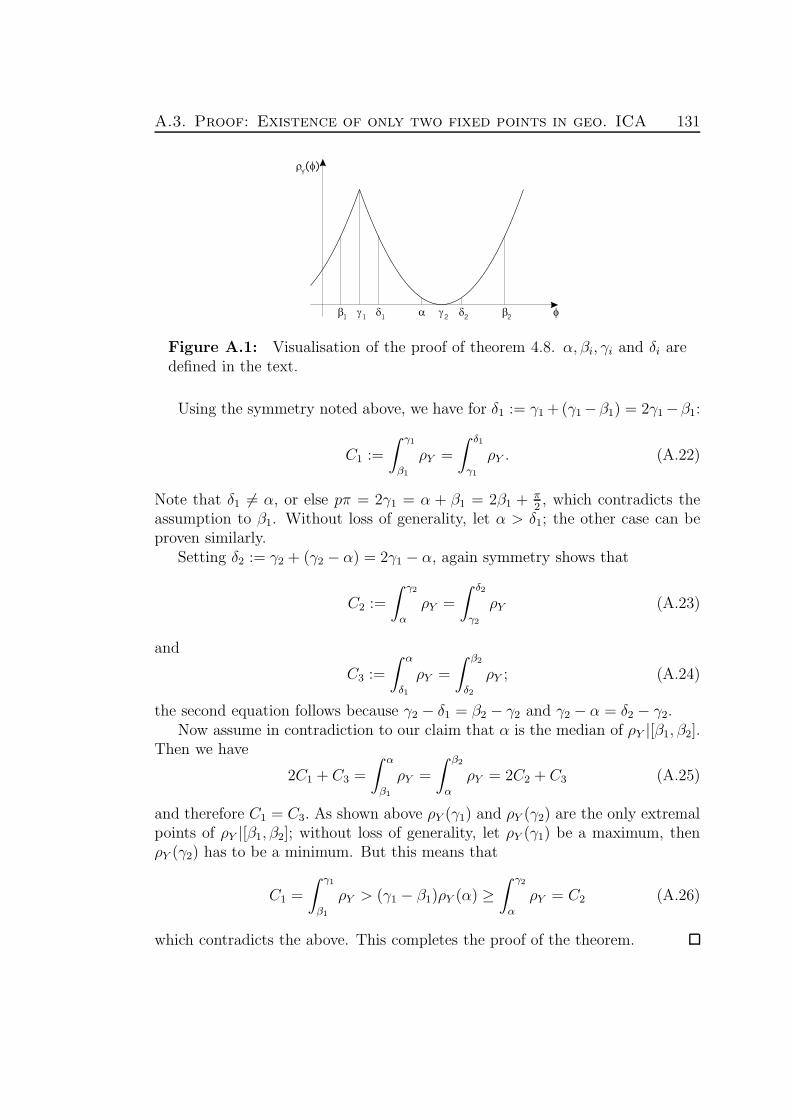
A.3. Proof: Existence of only two fixed points in geo. ICA 131
Figure A.1: Visualisation of the proof of theorem 4.8. α, βi, γi and δi aredefined in the text.
Using the symmetry noted above, we have for δ1 := γ1 +(γ1−β1) = 2γ1−β1:
C1 :=
∫ γ1
β1
ρY =
∫ δ1
γ1
ρY . (A.22)
Note that δ1 6= α, or else pπ = 2γ1 = α + β1 = 2β1 + π2, which contradicts the
assumption to β1. Without loss of generality, let α > δ1; the other case can beproven similarly.
Setting δ2 := γ2 + (γ2 − α) = 2γ1 − α, again symmetry shows that
C2 :=
∫ γ2
α
ρY =
∫ δ2
γ2
ρY (A.23)
and
C3 :=
∫ α
δ1
ρY =
∫ β2
δ2
ρY ; (A.24)
the second equation follows because γ2 − δ1 = β2 − γ2 and γ2 − α = δ2 − γ2.Now assume in contradiction to our claim that α is the median of ρY |[β1, β2].
Then we have
2C1 + C3 =
∫ α
β1
ρY =
∫ β2
α
ρY = 2C2 + C3 (A.25)
and therefore C1 = C3. As shown above ρY (γ1) and ρY (γ2) are the only extremalpoints of ρY |[β1, β2]; without loss of generality, let ρY (γ1) be a maximum, thenρY (γ2) has to be a minimum. But this means that
C1 =
∫ γ1
β1
ρY > (γ1 − β1)ρY (α) ≥∫ γ2
α
ρY = C2 (A.26)
which contradicts the above. This completes the proof of the theorem.


Bibliography
G. S. Adair. The oxygen dissociation curve of hemoglobin. Journal of BiologicalChemistry, LXIII:529–545, 1925.
S. Amari. Natural gradient works efficiently in learning. Neural Computation, 10(2):251–276, 1998.
S. Amari, A. Cichocki, and H. Yang. A new learning algorithm for blind signalseparation. Advances in Neural Information Processing Systems, 8:757–763,1996.
S.-I. Amari. Estimating functions of independent component analysis for tempo-rally correlated signals. Neural Computation, 12(9):2083–2107, 2000.
H. An, W. Lin, A. Celik, and Y. Z. Lee. Quantitative measurements of cerebralmetabolic rate of oxygen utilization using MRI: a volunteer study. NMR inBiomedicine, 14:441–447, 2001.
W. Bargmann. Histologie und mikroskopische Anatomie des Menschen. GeorgThieme Verlag, 7th edition, 1977.
C. Bauer, C. Puntonet, M. Rodriguez-Alvarez, and E. Lang. Separation of EEGsignals with geometric procedures. Engineering of Intelligent Systems (Proc.EIS’2000), pages 104–108, 2000.
A. Bekker, S. Wolk, H. Turndorf, D. Kristol, and A. Ritter. Computer simula-tion of cerebralvascular circulation: Assessment of intracranial hemodynamicsduring induction of anesthesia. Journal of Clinical Monitoring, 12:433–444,1996.
A. J. Bell and T. J. Sejnowski. An information-maximisation approach to blindseparation and blind deconvolution. Neural Computation, 7:1129–1159, 1995.
A. Belouchrani, K. A. Meraim, J.-F. Cardoso, and E. Moulines. A blind sourceseparation technique based on second order statistics. IEEE Trans. on SignalProcessing, 45(2):434–444, 1997.
133

134 Bibliography
M. Benaim, J.-C. Fort, and G. Pages. Convergence of the one-dimensional Ko-honen algorithm. Adv. Appl. Prob., 30:850–869, 1998.
Bosch. Statistik-Taschenbuch, pages 697–701. Oldenbuch Verlag, 2nd edition,1993.
A. Brawanski, R. Faltermeier, R. D. Rothoerl, and C. Woertgen. Comparison ofnear-infrared spectroscopy and tissue pO2 time series in patients after severehead injury and aneurysmal subarachnoid hemorrhage. Journal of CerebralBlood Flow & Metabolism, 22:605–611, 2002.
A. Cichocki and S. Amari. Adaptive blind signal and image processing. JohnWiley & Sons, 2002.
P. Comon. Independent component analysis: A new concept? Signal Processing,36:287–314, 1994.
M. Cottrell and J.-C. Fort. Etude d’un processus d’auto-organisation. Annalesde l’Institut Henri Poincare, 23(1):1–20, 1987. (in French).
M. Cottrell, J. C. Fort, and G. Pages. Two or three things that we know aboutthe Kohonen algorithm. In M. Verleysen, editor, European Symp. on ArtificialNeural Networks (Proc. ESANN’94), pages 235–244, Brussels, Belgium, 1994.
R. G. Crystal, J. B. West, P. J. Barnes, and N. S. Cherniack, editors. The Lung:Scientific Foundations, volume 2. Raven Press Ltd., New York, 1991.
M. Czosnyka, J. Pickard, H. Whitehouse, and S. Piechnik. The hyperaemicresponse to a transient reduction in cerebral perfusion pressure. Acta Neu-rochirurgica, pages 90–97, 1992.
M. Czosnyka, S. Piechnik, H. K. Richards, P. Kirkpatrick, P. Smielewski, andJ. D. Pickard. Contribution of mathematical modelling to the interpretationof bedside tests of cerebrovascular autoregulation. Journal of Neurology, Neu-rosurgery and Psychiatry, 63:721–731, 1997.
N. Delfosse and P. Loubaton. Adaptive blind separation of independent sources:a deflation approach. Signal Processing, 45:59–83, 1995.
H. G. Friden and J. Ekstedt. Volume/pressure relationship of the cerebrospinalspace in humans. Neurosurgery, 13(4):351–366, 1983.
M. R. Gaab, I. Haubitz, A. Brawanski, J. Faulstich, and H. E. Heißler. Intracra-nial Pressure V, chapter ”Pressure-Volume diagram, pulse amplitude and in-tracranial pulse volume - analysis and significance”. Springer Verlag, 1983.

Bibliography 135
E. Gao, W. L. Young, J. Pile-Spellman, E. Ornstein, and Q. Ma. Mathematicalconsiderations for modeling cerebral blood flow autoregulation to systemic ar-terial pressure. American Journal of Physiology 274 (Heart Circ. Physiol. 43),pages 1023–1031, 1998.
M. Gardner. Mathematical games: White and brown music, fractal curves andone-over-f fluctuations. Scientific American, 238(4):16–32, 1978.
M. Giulioni and M. Ursino. Impact of cerebral perfusion and autoregulationon intracranial dynamics: A modeling study. Neurosurgery, 39(5):1005–1015,November 1996.
E. M. Golding, C. S. Robertson, and R. M. Bryan. The consequences of traumaticbrain injury on cerebral blood flow and autoregulation: A review. Clinical andExperimental Hypertension, 21(4):299–332, 1999.
R. Greger and U. Windhorst. Comprehensive Human Physiology, volume 2.Springer Verlag, 1996.
A. V. Hill. The possible effects of the aggregation of the molecules of hemoglobinon its dissociation curves. Journal of Physiology, XL:iv–vii, 1910.
O. Hoffmann. Biomathematics of intracranial CSF and haemodynamics. Simula-tion and analysis with the aid of a mathematical model. Acta Neurochirurgica,40:117–130, 1987.
L. Hoofd. Oxygen transport in biological systems: modeling of pathways fromenviroment to cell, chapter ”Updating the Krogh model – assumptions andextensions”, pages 197–229. Press Syndicate of the University of Cambridge,1992.
S. Hosseini and C. Jutten. Blind seperation of temporally correlated sourcesusing a quasi maximum likelihood approach. Independent Component Analysisand Blind Signal Separation (Proc. ICA2001) - Proceedings, San Diego, USA,2001.
A. G. Hudetz, J. H. Hasley, C. R. Horton, K. A. Conger, and D. D. Reneau.Mathematical simulation of cerebral blood flow in focal ischemia. Stroke, 13(5), 1982.
A. Hyvarinen. Fast and robust fixed-point algorithms for independent componentanalysis. IEEE Trans. on Neural Networks, 10(3):626–634, 1999.
A. Hyvarinen, J. Karhunen, and E. Oja. Independent Component Analysis. JohnWiley & Sons, 2001.

136 Bibliography
A. Hyvarinen and E. Oja. A fast fixed-point algorithm for independent componentanalysis. Neural Computation, 9:1483–1492, 1997a.
A. Hyvarinen and E. Oja. Independent component analysis by general nonlinearhebbian-like learning rules. Signal Processing, 64(3):301–313, 1997b.
A. Jung and A. Kaiser. Considering temporal structures in independent compo-nent analysis. Independent Component Analysis and Blind Signal Separation(Proc. ICA 2003) - Nara, Japan, 2003.
A. Jung, F. J. Theis, C. G. Puntmnet, and E. W. Lang. FastGeo – A histogrambased approach to linear geometric ICA. Independent Component Analysis andBlind Signal Separation (Proc. ICA2001), San Diego, USA, 2001.
C. Jutten and J. Herault. Blind separation of sources, part I: An adaptive algo-rithm based on neuromimetic architecture. Signal Processing, 24:1–10, 1991.
Z. M. Kadas, W. D. Lakin, J. Yu, and P. L. Penar. A mathematical mdel ofthe intracranial system including autoregulation. Neurological Research, 19:441–450, 1997.
A. Kaiser. Nichtlineare Methoden zur Quantifizierung von Abhangigkeiten undKopplungen zwischen stochastischen Prozessen basierend auf Informationsthe-orie. PhD thesis, Universitat Wuppertal, 2002.
A. Kaiser and T. Schreiber. Information transfer in continuous processes. PhysicaD, 166:43–62, 2002.
H. Kantz and T. Schreiber. Nonlinear Time Series Analysis. Cambridge Univer-sity Press, 1997.
F. U. Kauper. Transkranielle Oximetrie mittels Nahinfrarotspektroskopie. PhDthesis, Universitat Erlangen, 1999.
M. B. Kim, D. S. Ward, C. R. Cartwright, J. Kolano, S. Chlebowski, and L. C.Henson. Estimation of jugular venous O2 saturation from cerebral oximetry orarterial O2 saturation during isocapnic hypoxia. Journal of Clinical Monitoringand Computing, 16:191–199, 2000.
R. Klinke and S. Silbernagl. Lehrbuch der Physiologie. Georg Thieme Verlag, 4thedition, 2003.
A. Krogh. The number and distribution of capillaries in muscles with calculationsof the oxygen pressure head necessary for supplying the tissue. Journal ofPhysiology, LII:409–415, 1918-1919.
Bibliography 137
J. Kugler. Elektroenzephalographie in Klinik und Praxis – Eine Einfuhrung. GeorgThieme Verlag, 1981.
W. D. Lakin, J. Yu, and P. Penar. Mathematical modeling of pressure dynamicsin the intracranial system. Nova Journal of Mathematics, Game Theory andAlgebra, 5(2):103–130, 1996.
T. Lee. Independent Component Analysis – Theory and Applications. KluwerAcademic Publishers, 1998.
T.-W. Lee, M. Girolami, and T. Sejnowski. Independent component analysis us-ing an extended infomax algorithm for mixed sub-gaussian and super-gaussiansources. Neural Computation, 11:417–441, 1999.
M. Lewicki and T. Sejnowski. Learning nonlinear overcomplete representationsfor efficient coding. In Advances in Neural Information Processing System,volume 10. The MIT Press, 1998.
R. Linsker. Local synaptic learning rules suffice to maximize mutual informationin a linear network. Neural Computation, 4:691–702, 1992.
K. Matsuoka, M. Ohya, and M. Kawamoto. A neural net for blind separation ofnonstationary signals. Neural Networks, 8(3):411–419, 1995.
G. I. Mchedlishvili. Arterial behaviour and blood circulation in the brain. PlenumPress, New York, 1986.
G. Meier. Untersuchung nichtlinearer Zeitreihenanalysemethoden. Diplomarbeit- Universitat Regensburg, March 2000.
C. Metz. Vergleichende untersuchungen zur morbiditat und mortalitat bei arte-ria carotis endarteriektomien in allgemeinanasthesie versus regionalanasthesieunter besonderer berucksichtigung der zerebralen ischaemie. Habilitation -Universitat Regensburg, 2001.
M. A. Mintun, B. N. Lundstrom, A. Z. Snyder, A. G. Vlassenko, G. L. Shulman,and M. E. Raichle. Blood flow and oxygen delivery to human brain duringfunctional activity: Theoretical modeling and experimental data. Proceedingsof the National Academy of Sciences, 98(12):6859–6864, 2001.
L. Molgedey and H. Schuster. Separation of a mixture of independent signalsusing time delayed correlations. Physical Review Letters, 72:3634–3636, 1994.
E. Okada, M. Firbank, M. Schweiger, S. R. Arridge, M. Cope, and D. T. Delpy.Theoretical and experimental investigation of near-infrared light propagationin a model of the adult head. Applied Optics, 36(1):21–31, 1997.
138 Bibliography
A. Papoulis. Probability, Random Variables and Stochastic Processes. McGraw-Hill, 3rd edition, 1991.
R. K. Pathria. Statistical Mechanics, pages 504–505. Butterworth, Heinemann,2nd edition, 1998.
B. Pearlmutter and L. Parra. Maximum likelihood blind source separation: Acontext-sensitive generalization of ICA. Advances in Neural Information Pro-cessing Systems, 1997.
A. Prieto, B. Prieto, C. Puntonet, A. Canas, and P. Martin-Smith. Geometricseparation of linear mixtures of sources: Application to speech signals. In-dependent Component Analysis and Blind Signal Separation (Proc. ICA’99),pages 295–300, 1999.
C. Puntonet, M. Alvarez, A. Prieto, and B. Prieto. Separation of speech signalsfor nonlinear mixtures. Lecture Notes in Computer Science, 1607:665–673,1999.
C. Puntonet, C. Bauer, E. Lang, M. Alvarez, and B. Prieto. Adaptive-geometricmethods: Application to the separation of EEG signals. Independent Compo-nent Analysis and Blind Signal Separation (Proc. ICA’2000), pages 273–278,2000.
C. Puntonet and A. Prieto. An adaptive geometrical procedure for blind separa-tion of sources. Neural Processing Letters, 2(5), 1995.
C. G. Puntonet and A. Prieto. Neural net approach for blind separation of sourcesbased on geometric properties. Neurocomputing, 18:141–164, 1998.
C. G. Puntonet, A. Prieto, C. Jutten, M. R. Alvarez, and J. Ortega. Separationof sources: a geometry-based procedure for reconstruction of n-valued signals.Signal Processing, 46:267–284, 1995.
M. J. Purves. The Physiology of the Cerebral Circulation. Cambirdge UniversityPress, 1972.
U. Raff, A. L. Scherzinger, P. F. Vargas, and J. H. Simon. Quantitation ofgrey matter, white matter, and cerebrospinal fluid from spin-echo magneticresonance images using artificial neural network techniques. Medical Physics,21(12):1933–1942, 1994.
D. D. Reneau, D. F. Bruley, and M. H. Knisely. Chemical Engineering in Med-incine and Biology, chapter ”A mathematical simulation of oxygen release,diffusion, and consumption in the capillaries and tissue of the human brain”,pages 135–241. Plenum Press, New York, 1967.

Bibliography 139
D. D. Reneau, D. F. Bruley, and M. H. Knisely. A digital simulation of transientoxygen transport in capillary-tissue systems (cerebral grey matter). AIChEJournal, 15(6):916–925, November 1969.
D. D. Reneau, D. F. Bruley, and M. H. Knisely. A computer simulation for predic-tion of oxygen limitations in cerebral gray matter. Journal of the Associationfor the Advancement of Medical Instrumentation, 4(6):211–223, 1970.
D. D. Reneau and M. H. Knisely. A mathematical simulation of oxygen trans-port in the human brain under conditions of countercurrent capillary bloodflow. Advances in Bioengineering – Chemical Engineering Progress SymposiumSeries, 67(114):18–27, 1971.
H. Ritter and K. Schulten. Convergence properties of Kohonen’s topology con-serving maps: Fluctuations, stability and dimension selection. Biological Cy-bernetics, 60:59–71, 1988.
F. J. W. Roughton and J. W. Severinghaus. Accurate determination of O2 disso-ciation curve of human blood above 98.7% saturation with data on O2 solubilityin unmodified human blood from 0 to 37 C. Journal of Applied Physiology,35(6):861–869, December 1973.
R. F. Schmidt, G. Thews, and F. Lang. Physiologie des Menschen. SpringerVerlag, 28th edition, 2000.
T. Schreiber. Measuring information transfer. Physical Review Letters, 85:461,2000.
J. W. Severingshaus. Simple, accurate equations for human blood O2 dissociationcomputations. Journal of Applied Physiology, 46:599–602, January-June 1979.
M. Sharan and A. S. Popel. A compartment model for oxygen transport in brainmicrocirculation in the presence of blood substitutes. Journal of theoreticalBiology, 216:479–500, 2002.
F. H. Sklar and I. Elashvili. The pressure-volume function of brain elasticity –physiological considerations and clinical applications. Journal of Neurosurgery,47:670–679, 1977.
S. A. Stevens. Mean pressures and flows in the human intracranial system, deter-mined by mathematical simulations of a steady-state infusion test. NeurologicalResearch, 22:809–814, 2000.
H. G. Sullivan and J. D. Allison. Physiology of cerebrospinal fluid. In R. Wilkinsand S. Rengachary, editors, Neurosurgery, volume 3, pages 2125–2135. McGrawHillbook Co., New York, 1985.

140 Bibliography
F. Theis, E. Lang, and C. Puntonet. A geometric algorithm for overcompletelinear ICA. Neurocomputing, 2003a. accepted.
F. J. Theis. Mathematics in Independent Component Analysis. PhD thesis,University Regensburg, 2002.
F. J. Theis, A. Jung, and E. W. Lang. A theoretic model for linear geometricICA. Independent Component Analysis and Blind Signal Separation (Proc.ICA2001), San Diego, USA, 2001.
F. J. Theis, A. Jung, C. G. Puntonet, and E. W. Lang. Linear geometric ICA:Fundamentals and algorithms. Neural Computation, 15:419–439, 2003b.
L. Tong, R.-W. Liu, V. Soon, and Y. Huang. Indeterminacy and identifiability ofblind identification. IEEE Trans. on Circuits and Systems, 38:499–509, 1991.
M. Ursino. A mathematical study of human intracranial hydrodynamics: Part1 - The cerebrospinal fluid pulse pressure. Annals of Biomedical Engineering,16:379–401, 1988.
M. Ursino and C. Lodi. A simple mathematical model of the interaction be-tween intracranial pressure and cerebral hemodynamics. Journal of AppliedPhysiology, 82(4):1256–1269, 1997.
S. Wiggins. Introduction to Applied Nonlinear Dynamical Systems and Chaos.Springer Verlag, 1990.
C. Woertgen, R. Faltermeier, R. Rothorl, and A. Brawanski. Vergleich von ven-rikelnahen und kortikalen intracraniellen drucken. In Jahrestagung der SektionIntracranieller Druck, Hirndurchblutung, Hirnodem der Deutschen Gesellschaftfur Neurochirurgie, Berlin, Unfallkrankenhaus, 10.-11.Oktober 2003.
A. Ziehe and K.-R. Muller. TDSEP – an efficient algorithm for blind sepa-ration using time structure. Proc. Int. Conf. on Artificial Neural Networks(ICANN’98), pages 675–680, 1998. Skovde, Sweden.
S. Zschocke. Klinische Elektroenzephalographie. Springer Verlag, 1995.
A. Zwart, G. Kwant, B. Oeseburg, and W. G. Zijlstra. Human whole-bodyoxygen affinity: effect of temperature. Journal of Applied Physiology, 57:429–434, July-December 1984.

Dank
Ich mochte mich besonders bei den folgenden Personen bedanken, die diese Arbeitin dieser Form moglich gemacht haben. Speziell geht mein Dank an meinenDoktorvater und Betreuer Klaus Richter, da ohne ihn diese Arbeit nicht hier– lieber Leser – in ihren Handen liegen wurde.
Fur die Unterstutzung und Hilfe als wichtiges Glied zwischen Physik undMedizin bedanke ich mich bei Rupert Faltermeier der auch innerhalb kurzesterZeit die verschiedensten Versionen meiner Dissertation korregiert hat. Bei RalfRothorl mochte ich mich fur die manchmal fur ihn etwas anstrengenden medi-zinischen Diskussionen bedanken, wie auch bei Professor Brawanski fur die im-mer wahrende Unterstutzung zum Fortfuhren der Arbeit im medizinischen Ge-biet. Aber ebenso bei Professor Gustav Obermair, der die Kooperation zwischenMedizin und Physik erst initiiert hat und damit an der Entstehung dieses Teilsder Arbeit wesentlich beigetragen hat.
Dank auch an Andreas Kaiser, ohne ihn der ICA Teil nicht seine jetzige Formhatte und mir immer geduldig meine Fragen bzgl. Wahrscheinlichkeits- und Infor-mationstheorie beantwortet hat. Ebenso aber auch Fabian Theis fur die Zusam-menarbeit und Diskussionen auf dem Gebiet der (geometrischen) ICA und furdie fur uns beide interessanten Konferenzreisen.
Jorg Kaidel danke ich fur die vielen Ratschlage und Diskussionen, speziellwahrend der Entstehung dieser Arbeit – operation ”falling snow” ist also dochnoch punktlich fertig geworden. Meinem Zimmerkollegen Juan-Diego Urbinadank ich ebenfalls, speziell fur die Hilfe bei den vielen ”illposed questions” –wie er sie immer nannte – und Peter Schlagheck fur das geduldige Zuhoren beimeinen Problemen mit der Dissertation. Ausserdem danke ich Gustav Mecke furdie Arbeit als grundlicher Lektor.
Fur die professionelle EDV-Unterstutzung mochte ich mich besonders bei FritzWunsch und Rudi Holzer bedanken, die fur unsere Probleme immer ein offenesOhr hatten. Aber auch Christian Guggenberger, der uns unermudlich bei un-serem Physik-Cluster und allen anderen Probleme von Linux geholfen hat. Dankauch an Christoph Bauer, der einerseits mich an Anfang an der Uni und in Re-gensburg willkommen geheissen hat, aber auch jetzt sich sehr um die Belange derPhysik im Rechenzentrum kummert. Ausserdem Dank an meine EDV-KollegenJosef Kainz und Christian Lechner fur die herzliche Atmosphare.
141

142 Dank
Der Deutschen Forschungsgemeinschaft danke ich fur die finanzielle Unterstut-zung im Rahmen eines Stipendiums im Graduiertenkolleg ”Nichtlinearitat undNichtgleichgewicht in kondensierter Materie”.
Naturlich hat die angenehme und warme Atmosphare am Institut ebenfallszu der glucklichen Entstehung der Arbeit beigetragen, daher Dank an alle Mitar-beiter am Institut. Besonders danke ich aber Angela Reißer, die ich immer alshilfsbereite und liebe Sekretarin erleben durfte.
Doch ohne die Liebe und Unterstutzung meiner Eltern ware diese Arbeit nieentstanden. Danke!
Allen nochmal herzlichen Dank, auch jenen,die aus reiner Vergesslichkeit hier nicht aufgefuhrt sind.