Statistial mechanics& free energy methods

Tutoriel CPMD/CP2KParis, 6–9 avril 2010

François-Xavier Coudert

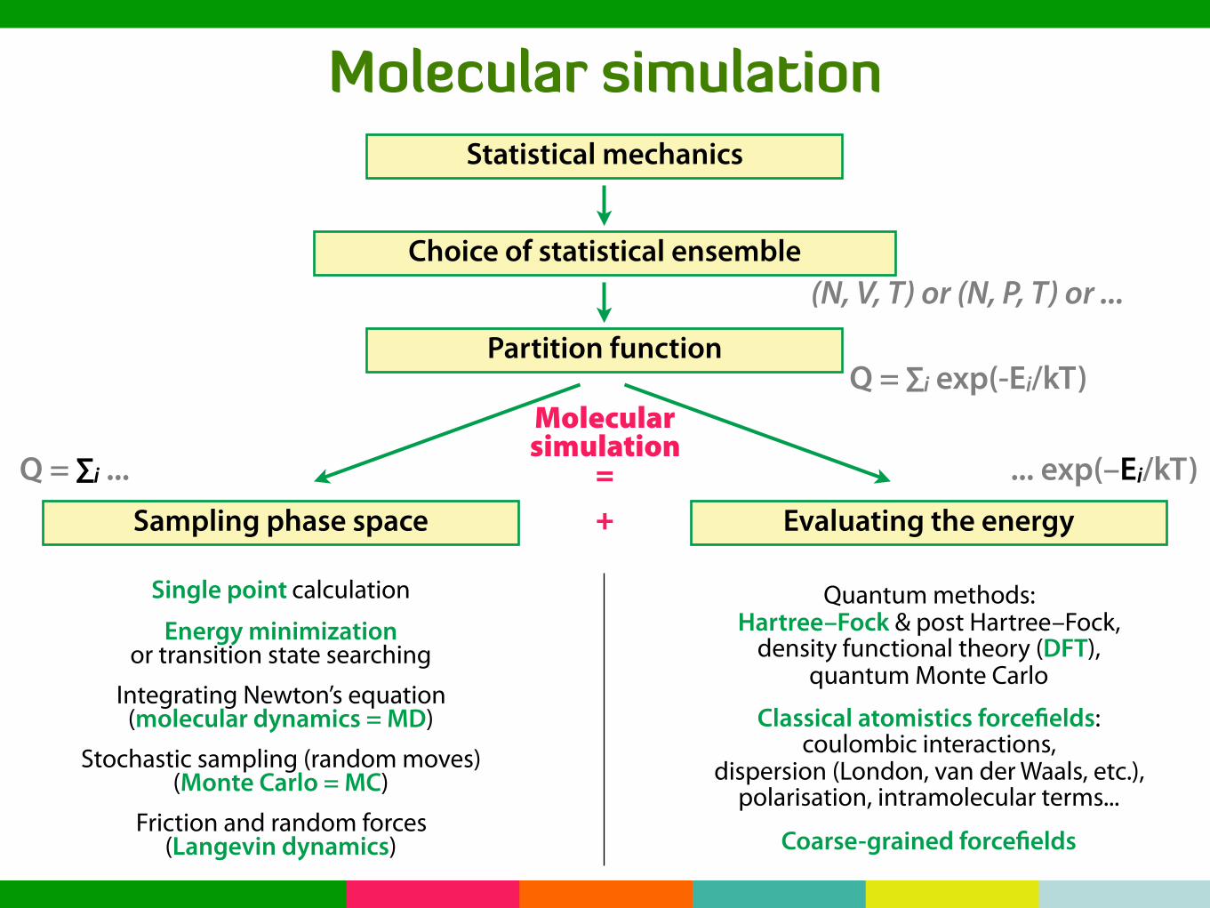
Molecular simulationStatistical mechanics

Choice of statistical ensemble

Partition function

(N, V, T) or (N, P, T) or ...

Q = ∑i exp(-Ei/kT)

Sampling phase space Evaluating the energy

Molecularsimulation

=+

Q = ∑i ... ... exp(–Ei/kT)

Single point calculation

Energy minimizationor transition state searching

Integrating Newton’s equation(molecular dynamics = MD)

Stochastic sampling (random moves)(Monte Carlo = MC)

Friction and random forces(Langevin dynamics)

Quantum methods:Hartree–Fock & post Hartree–Fock,

density functional theory (DFT),quantum Monte Carlo

Classical atomistics forcefields:coulombic interactions,

dispersion (London, van der Waals, etc.),polarisation, intramolecular terms...

Coarse-grained forcefields

Molecular simulationSampling phase space

Monte-Carlo Molecular dynamics

to calculate observables as averages on a large number of configurations

P ∝ e−βE

Trajectories

Dynamical processes

Collective moves

Randommoves

Many statisticalensembles

Nonlocalsampling

A=a=

ai

N= lim

t→∞

a(τ)dτ

tm r = −∂V

∂r

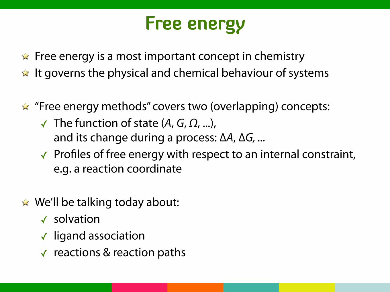
Free energyFree energy is a most important concept in chemistryIt governs the physical and chemical behaviour of systems

“Free energy methods” covers two (overlapping) concepts: The function of state (A, G, ΩΩ, ...),

and its change during a process: ∆A, ∆G, ... Profiles of free energy with respect to an internal constraint,

e.g. a reaction coordinate

We’ll be talking today about: solvation ligand association reactions & reaction paths

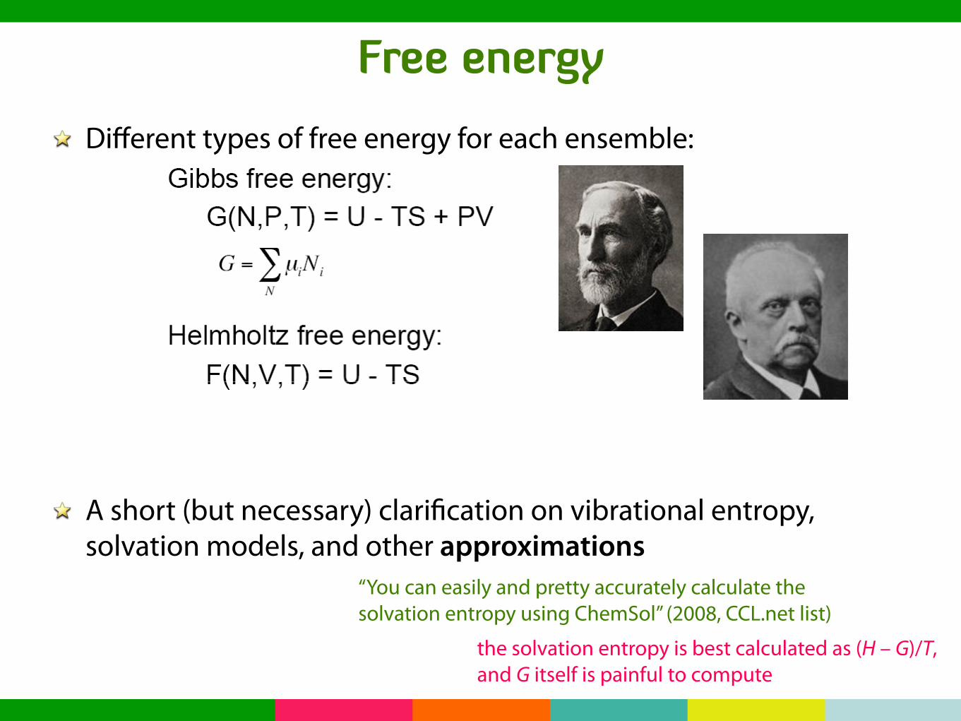
Free energyDifferent types of free energy for each ensemble:

A short (but necessary) clarification on vibrational entropy,solvation models, and other approximations

“You can easily and pretty accurately calculate the solvation entropy using ChemSol” (2008, CCL.net list)

the solvation entropy is best calculated as (H – G)/T, and G itself is painful to compute

Free energy

When you’re using local approximations for the free energy,are you positive your potential energy surface doesn’t look like this?

•First •Prev •Next •Last •Go Back •Full Screen •Close •Quit

Unforeseen Stationary States

• ... or what if the potential energy landscape is very rugged?

• Dynamical bottleneck and diffusive barriers

• Many irrelevant saddle points

Free energy methodsWe will talk today about:

Thermodynamic perturbation& thermodynamic integration

Umbrella sampling

Adiabiatic free energy sampling

Metadynamics

One word about collective variablesThey can be: distances angles simulation box parameters coordination numbers etc.

Thermodynamic perturbation

Zwanzig, 1954:

Some conditions have to be met: States A and B have to be “close” i.e. they should have widely overlapping phase space basins i.e. EA – EB should always be ≤ kT

As such, not very useful... How do we solve that?

Thermodynamic perturbation

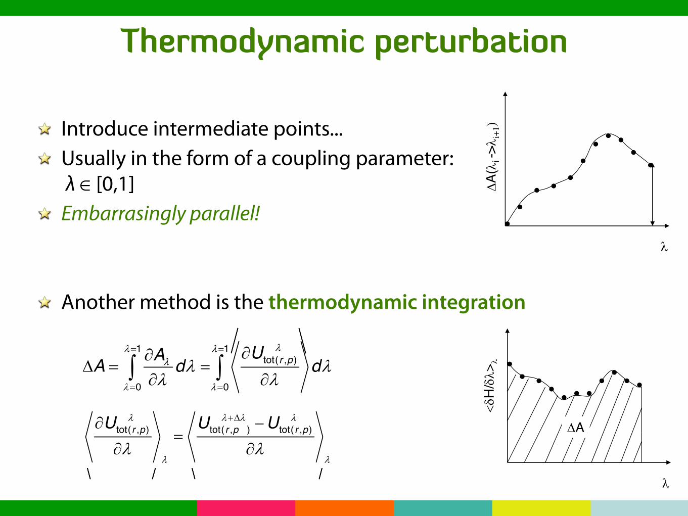
Introduce intermediate points...Usually in the form of a coupling parameter: λ ∈ [0,1]Embarrasingly parallel!

Another method is the thermodynamic integrationThermodynamical integration method (TI)

!! !" " ##1 1 UA

Thermodynamical integration method (TI)

!

! !

! !! !" "

##$ " "

# #% % tot( , )

0 0

r pUAA d d

! ! ! !

! !

&$# '"

# #tot( , ) tot( , ) tot( , )r p r p r pU U U

! !! !# #

Thermodynamical integration method (TI)

!! !" " ##1 1 UA

Thermodynamical integration method (TI)

!

! !

! !! !" "

##$ " "

# #% % tot( , )

0 0

r pUAA d d

! ! ! !

! !

&$# '"

# #tot( , ) tot( , ) tot( , )r p r p r pU U U

! !! !# #

Two approaches of free energy calculationqthermodynamicalPerturbation Thermodynamical Intégration

! i+1

)

"!> !

#A(! i

->

#A

$"H

/"! !! !

Two approaches of free energy calculationqthermodynamicalPerturbation Thermodynamical Intégration

! i+1

)

"!> !

#A(!

i ->

#A

$"H

/"

! !! !

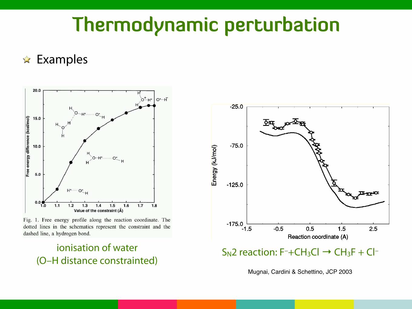
Thermodynamic perturbationExamples

•First •Prev •Next •Last •Go Back •Full Screen •Close •Quit

Autoionization of Liquid WaterContraint: O∗ −H∗ distance

ionisation of water(O–H distance constrainted)

•First •Prev •Next •Last •Go Back •Full Screen •Close •Quit

SN2 reaction F−

+CH3Cl→ CH3F + Cl−

Mugnai, Cardini & Schettino, JCP 2003

• Left: (Free) energy profile along the reaction paths at 0 and 300 K

• Right: Dipole moment CH3X and Y−

along the 0 K reaction path

SN2 reaction: F–+CH3Cl → CH3F + Cl–

Mugnai, Cardini & Schettino, JCP 2003

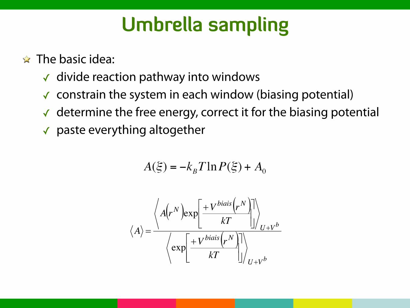
Umbrella samplingThe basic idea: divide reaction pathway into windows constrain the system in each window (biasing potential) determine the free energy, correct it for the biasing potential paste everything altogether

Calculation of average quantitiesAverage values obtained through biased simulations are corrected

! "

Average values obtained through biased simulations are corrected

! " ! "b

NbiaisN

kTrVrA

##$

%

&&'

()exp

! "b

NbiaisVU

rVA )

#%

&()

#$&'*

expbVU

kT)#

#$&

&'

exp

Umbrella samplingExample: PMF for internal rotation of the chromophore in GFP

courtesy of I. Demachy, Paris-Sud 11

ExampleExample Calculation of the free energy variation

along the internal rotation of the chromophoreIn Green Fluorescent ProteinIn Green Fluorescent Protein

Practical aspectsPractical aspects

Successive biased simulationsPractical aspectsPractical aspects

Successive biased simulations

Adiabatic free energy samplingThe basic idea: define reaction coordinates and environment coordinates give the reaction coordinates a large effective mass

(the environment coordinates will follow adiabatically) thermostate the reaction coordinates at high temp.

(so that the free energy profile is fully sampled)

Adiabatic free energy samplingExample:

•First •Prev •Next •Last •Go Back •Full Screen •Close •Quit

Conversion of 2-Bromoethanol to Dibromoethane

The heavy atoms of the bromoethanol molecule are taken as the reactive sub-

system (masses scaled by 100, coupled to a Nose-Hoover at T=2000 K). Solute

and H at 300 K, QM/MM setup

protonated torsion bromonium ion

Free exploration of configurations

C-O distance1 4

angle

60

110 C-C-O

Br-C-C

dissociation

and

bromonium

concerted

from 2-bromoethanolto dibromoethane

Br, C, C, O coordinates are the reaction coordinates

J. VandeVondele and U. Rothlisberger,J. Phys. Chem. B 2002

QM/MM simulation

Theavy = 2000 KMheavy: scaled by 100

The basic idea: choose collective variables s history-dependent potential

biasing the simulation not tocome back too often to visitedmicrostates

Metadynamics

Metadynamics

cyclohexaneconformation changes

alanine dipeptide ψ/φ

movies by Vojtěch Spiwok

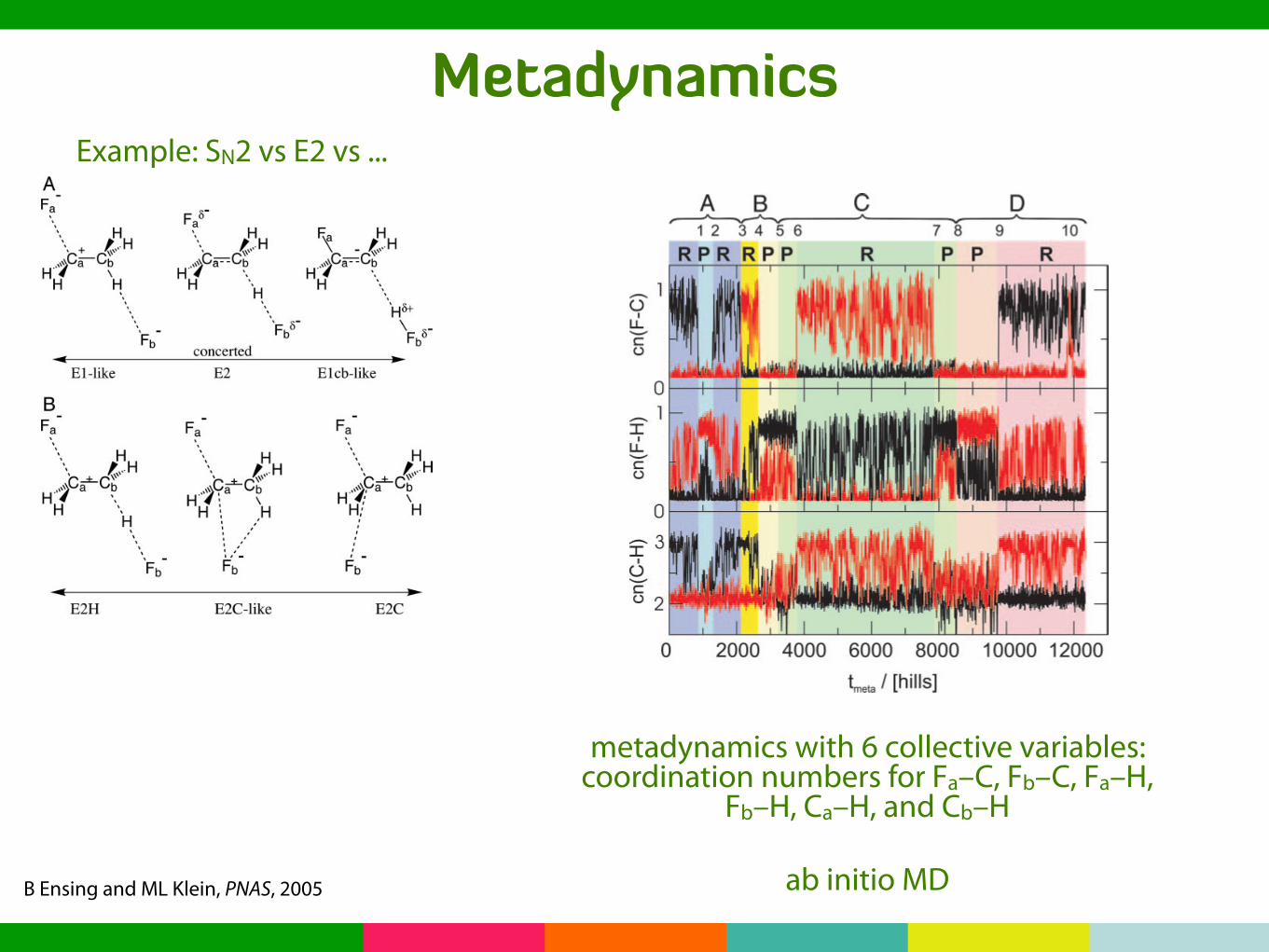
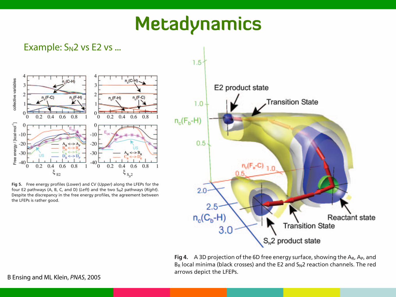
MetadynamicsExample: SN2 vs E2 vs ...

B Ensing and ML Klein, PNAS, 2005

the US technique to converge the free energy profile along theLFEP (6).

In the current study, the set of CV is extended with anotherthree coordinates, which allows us also to map out the competingSN2 reaction channel in the exploration of the free energylandscape and understand why traditional methods fail to obtainthe free energy profiles of the E2 and SN2 reaction channels.

Disregarding the change of the C–C bond, from single intodouble, during the E2 reaction between fluoroethane and thefluoride ion, there are three chemical bonds that are broken orformed during the reaction, namely, the Fa–Ca and a Cb–H bondsare broken, and a Fb–H bond is being formed. The chemicallyintuitive choice for the CV therefore would be the bond distancesof these three bonds, d(Fa ! C), d(Fb ! H), and d(Cb ! H).However, problems arise with this choice of CV, because even-tually the attacking Fb would abstract one of the other twohydrogens than the one prefixed by our choice of the Cb–H andFb–H bond distances. This alternative reaction almost certainlywould occur during a hills simulation after the first recrossing,when the attractive product free energy well already has beenfilled up with hills, so that the system escapes to these chemicallyequivalent but unintended product states. The problem is thatthe latter product states are indicated to be reactant states by theCb–H and Fb–H CV so that hills are being misplaced in CV space.

The problem would be solved by adding the other four Cb–Hand Fb–H bond distances to the set of CV. However, thesampling of the now seven-dimensional free energy surface iscomputationally very much more demanding than sampling ofthe initial 3D surface at the same accuracy. Alternatively, theproblem is overcome by considering the three coordinationnumbers, nc(Fa ! C), nc(Fb ! H), and nc(Cb ! H), where H andC denote all the hydrogen and carbon in the system, respectively.The coordination number is a function of the relevant bonddistance and is defined as

nc"A ! B# " !B

1 ! "d"A ! B#

d0#n

1 ! "d"A ! B#

d0#m. [1]

This function estimates the number of atoms B within the cutoffradius d0 of atom A (n and m are positive integers that determinehow ‘‘fast’’ the function goes from 1 to 0 at the cutoff radius r0).

Previously, we have computed successfully the 3D free energysurface for the E2 reaction by using the three coordinationnumbers as the CV (6). The reactant complex state is describedby the values nc(Fa–C) $ 1, nc(Fb–H) $ 0, nc(Cb–H) $ 3, andthe product complex state is defined by the values nc(Fa–C) $0, nc(Fb–H) $ 1, nc(Cb–H) $ 2. We applied the hills method toconstruct the 3D free energy surface. The LFEP and the USpotential were obtained from the sum of hills after having filledup the reactant and product wells with hills. The 1D free energyprofile was converged by using US.

Alternatively, the free energy surface can in principle beconverged to arbitrary accuracy within the hills method, by usingsmall enough hills and sampling many barrier recrossings (10).In practice, however, not only is converging the 3D surface morecostly than converging the 1D profile, but also, the efficiency ofthe hills method decreases as the accumulating hills grant accessto more and more of the higher-energy regions of configurationspace. For the E2 reaction, eventually this hills simulation endedwhen the free energy exploration stranded in a new localminimum by means of the SN2 attack of Fb on Ca while Fa wasleaving and forming a hydrogen bond with one of the #-hydro-gens. Escaping from this minimum requires the additional CVnc(Fb ! C) to break the newly formed Fb–Ca bond. Note that theSN2 channel leads to a product state that is chemically identicalto the initial state; only Fa and Fb have been exchanged.Returning via the SN2 channel from this product state istherefore less probable than proceeding with a ‘‘new’’ E2reaction, now with Fb as the leaving group and Fa as the attackingbase. A proper description of this step thus requires also theadditional nc(Fa ! H) CV. Finally, a rotation of the E2 leavinggroups FH and F! around C2H4 in the product state allowsexchange of Ca and Cb, so that also the nc(Ca ! H) needs to beadded to the set as the sixth CV.

In the present work, we compute the six-dimensional (6D) freeenergy surface by using the coordination numbers nc(Fa–C),nc(Fb–C), nc(Fa–H), nc(Fb–H), nc(Ca–H), and nc(Cb–H), whichallows us to study the E2 and the SN2 reactions simultaneously.

MethodsA 6D metadynamics CPMD simulation was performed by usingthe hills method algorithm, with a total length of 896,000 MDsteps (using a time step of 3 atomic units or 0.073 fs) to exploreand fill up the eight stable reactant and product wells. The heightof the Gaussian-shaped potential hills initially was set to 1

2kBT

(kBT % 1.68 kcal/mol), compared with an anticipated height ofthe barriers in the order of 10 kBT (11). Approximately halfwaythrough the exploration (after adding 5,600 hills), the height wasreduced to 1

4kBT to measure this effect on the efficiency and

accuracy of the free energy landscape exploration. A hill wasadded every 80 MD steps. The electronic wave function wasexpanded in plane waves up to an energy cut-off of 70 rydberg,in combination with Martin–Troullier type pseudopotentials.The Becke–Lee–Yang–Parr (BLYP) exchange-correlation den-sity functional was used. Further computational and technicaldetails of the computer simulations are found in the supportinginformation, which is published on the PNAS web site.

The LFEPs through the E2 and SN2 reaction channels wastraced in the resulting 6D free energy landscape by using amodified golden section algorithm as described in ref. 10.

Fig 1. Mechanistic spectra of possible TS of the bimolecular elimination (E2)reaction (A) and of the competing bimolecular nucleophilic substitution (SN2)reaction vs. E2 reaction channels (B).

6756 $ www.pnas.org%cgi%doi%10.1073%pnas.0408094102 Ensing and Klein

US simulations were performed by using the LFEPs !E2 and!SN2 as reaction coordinates. The estimate of the free energyalong the parameterized !, obtained from the sum of hills, wasused as the biasing potential. Additionally, overlapping har-monic window potentials were applied along ! to enhance andparallelize the sampling. The CV along the reaction coordinate,s(!), as well as the biasing potential, Ubias(!), and its derivatives,!s(!)Ubias, were computed a priori and read from file. Then, atevery CPMD time step, t, in the US simulation, the position ofthe system in 6D s(R) space is determined. The position alongthe reaction coordinate is estimated by taking

!"t# " min" !s"!# # s"R, t# !# , [2]

so that the biasing potential Ubias(!(t)) can be applied along withthe window potential. The resulting probability densities arefound in the supporting information, from which the finalconverged free energy profile was constructed by using theweighted histogram analysis method (12).

ResultsHere, we present our results of the calculation of the 6D freeenergy landscape of the E2 and SN2 reactions between fluoro-ethane and a fluoride ion. First, the results of the hills methodsimulation are presented. Then, the LFEPs of the E2 and SN2reaction channels are located, and, finally, we discuss the UScalculations of the 1D free energy profiles along the LFEPs ofthe two reaction mechanisms.

Exploring the 6D Free Energy Landscape. Exploration of a 6D freeenergy landscape is, even with the efficient hills method, verycomputationally demanding, so we cannot hope to converge theentire surface to chemical accuracy. Our focus is therefore on arough exploration of the 6D landscape and on visiting allrelevant stable states at least once. Then, in a second step, we willlocate the reaction channels and converge the 1D free energyprofile for the SN2 channel by US. Details of the E2 channel arecompared with our 3D exploration presented in ref. 6.

Fig. 2 shows the metadynamics of the six CV as a function ofthe number of hills added. The top image shows Fa leaving,following the E2 mechanism, after adding almost 1,000 hills, asindicated by the black line [i.e., initially nc(Fa–C) $ 1 switchingto nc(Fa–C) $ 0]. Simultaneously, the attacking Fb abstracts ahydrogen, indicated by the red line in the center image, whichinitially f luctuates with a large amplitude due to the Fb–H–Cb

Fig 2. Dynamics of the six CV shown as a function of the number of hills. (Top)The coordination numbers of C around Fa (black line) and Fb (red line). (Middle)The coordination numbers of H around Fa (black line) and Fb (red line).(Bottom) The coordination numbers of H around Ca (black line) and Cb (redline). The background colors blue, yellow, green, and red emphasize the fourdistinct E2 reactions (labeled A, B, C, and D at the top) that are sampled duringthe simulation, with the darker shades indicating the product states and thelighter shades indicating the reactant states (also denoted R and P on top).The numbers 1–10 at the top label the transitions and match the numbers inthe flow chart in Fig. 3.

Fig 3. Flow chart of the four E2 and two SN2 reactions between fluoroethaneand a fluoride ion, showing the eight stable states in boxes, with the reactantcomplexes AR, BR, CR, and DR at the left and the product complexes AP, BP, CP,and DP at the right. The connecting lines denote the transitions, with thenumbers between parentheses matching the numbers in Fig. 2 that label theoccurrence of the transition in the simulation. Dashed lines denote transitionsthat were not observed.

Ensing and Klein PNAS ! May 10, 2005 ! vol. 102 ! no. 19 ! 6757

CHEM

ISTR

YSP

ECIA

LFE

ATU

RE

metadynamics with 6 collective variables:coordination numbers for Fa–C, Fb–C, Fa–H,

Fb–H, Ca–H, and Cb–H

ab initio MD

MetadynamicsExample: SN2 vs E2 vs ...

B Ensing and ML Klein, PNAS, 2005

hydrogen bond in the reactant complex but increases to nc(Fb–H) ! 1 (with small oscillations) in the E2 product state, when HFis formed. In the bottom image, the black line indicates thedeparture of the hydrogen, as nc(Cb–H) switches from 3 to 2. Theother three CV are seen to be more or less inert thus far,although nc(Fa–H) (Center, black line) shows a small increase inthe E2 product state due to the formation of a hydrogen bondbetween the leaving group and ethylene.

The time that the system resides in the initial reactant state isindicated with a dark purple background, and the E2 productstate is contrasted with light blue. The number of hills requiredto fill up and escape the stable reactant state (!1,000) is an orderof magnitude higher compared with the 3D hills simulation (6),even though the fluctuations in the additional three CV are smalland the hills applied here are 1.6-fold larger.

This first transformation after the E2 mechanism is indicatedby a ‘‘1’’ at the top of Fig. 2. The label ‘‘2’’ marks the barrierrecrossing to the initial reactant state, after the first product stateis also filled with hills. The third transition occurs after adding!2,000 hills when Fb

" attacks the !-carbon, substituting theleaving group, Fa (note the interchange of the red and black linesin the top and center images indicating the SN2 reaction).

The different stable reactant and product states and theconnecting transformations are schematically represented in aflow chart, shown in Fig. 3. The four rows of boxes show the fourpossible E2 reaction pathways with the reactant states on the leftside and the product states on the right side. All four E2reactions were sampled in the hills method simulation and areindicated by the blue, yellow, green, and pink background colorsin Fig. 2. The first E2 reaction is labeled ‘‘A,’’ with a subscriptR or P denoting the reactant and product states, respectively, inthe flow chart. The initial reactant state (AR, e.g., recognized byFa leaving Ca) is connected to two ‘‘product’’ states in the flowchart, namely horizontally to AP via the E2 transformation andvertically to BR via the SN2 transformation. The numbers inparentheses shown at the connecting lines match the labeledtransformation events in Fig. 2.

Continuing after the SN2 reaction (marked ‘‘3’’ in Figs. 2 and 3),the BR state is filled with hills, after which Fa acts as the catalyzingbase, inducing the next E2 transformation (marked ‘‘4’’). From theBP product state the system does not recross. Instead, we observethe transfer of the HFa and Fb

" leaving groups around the ethylenemolecule, forming the CP product complex (marked ‘‘5’’). The CPstate is filled after adding almost 4,000 hills, after which a reverseE2 reaction brings the system to the CR ‘‘reactant’’ state. From CRthe system recrosses to CP (marked ‘‘7’’), after which anothersubstitution type of transformation takes place (marked ‘‘8’’). Thatis, the initially Cb hydrogen-bonded Fb

" transfers and forms ahydrogen bond to Ca. Then, it grabs the hydrogen, while simulta-neously HFa donates its proton back to Ca and transfers to form ahydrogen bond to Cb. Finally, the system moves from the DP to thelast E2 reactant state DR. From the DR state, we observe the SN2attack of Fb on Cb, but the system immediately recrosses back,because the CR state is apparently already completely filled withhills. After adding 12,300 hills (i.e., 106 MD steps or 120 ps), we endthe hills method simulation. Two transformations that were notsampled (a rotation and a hydrogen exchange), but can be inferredon symmetry grounds, are drawn with dashed connection lines inFig. 3.

LFEPs Through the E2 and SN2 Reaction Channels. The negative of thesum of hills placed in 6D CV space, although still far fromconverged, is a rough estimate of the underlying 6D free energylandscape. Unfortunately, it of course is not possible to easilyvisualize this result. We only can plot a hyperplane of the 6D freeenergy surface by taking three, four, or five CV to be constantor plot a projection by integrating over as many CV. Note thatto compute free energy differences between stable states orbetween reactant states and TS, integration over the well(s) isalways required, even for a 1D free energy profile.

Fig. 4 shows a 3D projection‡ of free energy isosurfaces, as afunction of nc(Fa " C), nc(Cb " H), and nc(Fb " H). The initialreactant state, AR, is found at the bottom right (1, 3, 0). Theellipsoid well has its long axis in the vertical nc(Fb " H)direction, indicating the easy Fb ! ! ! HCb hydrogen bond forma-tion, which preludes the E2 attack. The E2 product state is

‡The number of hydrogens on Ca is an inactive variable in the shown AR 3 AP and AR 3BR reactions (see also Fig. 2) so that it is chosen fixed at nc(Ca " H) # 2. The nc(Fa " H)and nc(Fb " C) are projected out in the remaining 5D surface.

Fig 4. A 3D projection of the 6D free energy surface, showing the AR, AP, andBR local minima (black crosses) and the E2 and SN2 reaction channels. The redarrows depict the LFEPs.

Fig 5. Free energy profiles (Lower) and CV (Upper) along the LFEPs for thefour E2 pathways (A, B, C, and D) (Left) and the two SN2 pathways (Right).Despite the discrepancy in the free energy profiles, the agreement betweenthe LFEPs is rather good.

6758 ! www.pnas.org"cgi"doi"10.1073"pnas.0408094102 Ensing and Klein

hydrogen bond in the reactant complex but increases to nc(Fb–H) ! 1 (with small oscillations) in the E2 product state, when HFis formed. In the bottom image, the black line indicates thedeparture of the hydrogen, as nc(Cb–H) switches from 3 to 2. Theother three CV are seen to be more or less inert thus far,although nc(Fa–H) (Center, black line) shows a small increase inthe E2 product state due to the formation of a hydrogen bondbetween the leaving group and ethylene.

The time that the system resides in the initial reactant state isindicated with a dark purple background, and the E2 productstate is contrasted with light blue. The number of hills requiredto fill up and escape the stable reactant state (!1,000) is an orderof magnitude higher compared with the 3D hills simulation (6),even though the fluctuations in the additional three CV are smalland the hills applied here are 1.6-fold larger.

This first transformation after the E2 mechanism is indicatedby a ‘‘1’’ at the top of Fig. 2. The label ‘‘2’’ marks the barrierrecrossing to the initial reactant state, after the first product stateis also filled with hills. The third transition occurs after adding!2,000 hills when Fb

" attacks the !-carbon, substituting theleaving group, Fa (note the interchange of the red and black linesin the top and center images indicating the SN2 reaction).

The different stable reactant and product states and theconnecting transformations are schematically represented in aflow chart, shown in Fig. 3. The four rows of boxes show the fourpossible E2 reaction pathways with the reactant states on the leftside and the product states on the right side. All four E2reactions were sampled in the hills method simulation and areindicated by the blue, yellow, green, and pink background colorsin Fig. 2. The first E2 reaction is labeled ‘‘A,’’ with a subscriptR or P denoting the reactant and product states, respectively, inthe flow chart. The initial reactant state (AR, e.g., recognized byFa leaving Ca) is connected to two ‘‘product’’ states in the flowchart, namely horizontally to AP via the E2 transformation andvertically to BR via the SN2 transformation. The numbers inparentheses shown at the connecting lines match the labeledtransformation events in Fig. 2.

Continuing after the SN2 reaction (marked ‘‘3’’ in Figs. 2 and 3),the BR state is filled with hills, after which Fa acts as the catalyzingbase, inducing the next E2 transformation (marked ‘‘4’’). From theBP product state the system does not recross. Instead, we observethe transfer of the HFa and Fb

" leaving groups around the ethylenemolecule, forming the CP product complex (marked ‘‘5’’). The CPstate is filled after adding almost 4,000 hills, after which a reverseE2 reaction brings the system to the CR ‘‘reactant’’ state. From CRthe system recrosses to CP (marked ‘‘7’’), after which anothersubstitution type of transformation takes place (marked ‘‘8’’). Thatis, the initially Cb hydrogen-bonded Fb

" transfers and forms ahydrogen bond to Ca. Then, it grabs the hydrogen, while simulta-neously HFa donates its proton back to Ca and transfers to form ahydrogen bond to Cb. Finally, the system moves from the DP to thelast E2 reactant state DR. From the DR state, we observe the SN2attack of Fb on Cb, but the system immediately recrosses back,because the CR state is apparently already completely filled withhills. After adding 12,300 hills (i.e., 106 MD steps or 120 ps), we endthe hills method simulation. Two transformations that were notsampled (a rotation and a hydrogen exchange), but can be inferredon symmetry grounds, are drawn with dashed connection lines inFig. 3.

LFEPs Through the E2 and SN2 Reaction Channels. The negative of thesum of hills placed in 6D CV space, although still far fromconverged, is a rough estimate of the underlying 6D free energylandscape. Unfortunately, it of course is not possible to easilyvisualize this result. We only can plot a hyperplane of the 6D freeenergy surface by taking three, four, or five CV to be constantor plot a projection by integrating over as many CV. Note thatto compute free energy differences between stable states orbetween reactant states and TS, integration over the well(s) isalways required, even for a 1D free energy profile.

Fig. 4 shows a 3D projection‡ of free energy isosurfaces, as afunction of nc(Fa " C), nc(Cb " H), and nc(Fb " H). The initialreactant state, AR, is found at the bottom right (1, 3, 0). Theellipsoid well has its long axis in the vertical nc(Fb " H)direction, indicating the easy Fb ! ! ! HCb hydrogen bond forma-tion, which preludes the E2 attack. The E2 product state is

‡The number of hydrogens on Ca is an inactive variable in the shown AR 3 AP and AR 3BR reactions (see also Fig. 2) so that it is chosen fixed at nc(Ca " H) # 2. The nc(Fa " H)and nc(Fb " C) are projected out in the remaining 5D surface.

Fig 4. A 3D projection of the 6D free energy surface, showing the AR, AP, andBR local minima (black crosses) and the E2 and SN2 reaction channels. The redarrows depict the LFEPs.

Fig 5. Free energy profiles (Lower) and CV (Upper) along the LFEPs for thefour E2 pathways (A, B, C, and D) (Left) and the two SN2 pathways (Right).Despite the discrepancy in the free energy profiles, the agreement betweenthe LFEPs is rather good.

6758 ! www.pnas.org"cgi"doi"10.1073"pnas.0408094102 Ensing and Klein

Reading

•First •Prev •Next •Last •Go Back •Full Screen •Close •Quit

Some Literature

• Blue Moon ensemble theory: G. Ciccotti et al. J. Chem. Phys. 109, 7737

(1998) and ref. therein

• Hessian based methods: eigenvalue following, dimer method.

• Nudged elastic band: G. Henkelman and H. Jonsson, J. Chem. Phys. 111,

7010 (1999).

• String method:W. E, W. Ren, and E. Vanden-Eijnden, Phys. Rev. B 66,

052301 (2002).

• Adaptive bias potential: van Gunsteren et al. J. Comput. 8, 695 (1994)

• Accelerated dynamics: A. Voter, J. Chem. Phys. 106 (11), 4665 (1997)

• Flooding potential: H. Grubmueller Phys. Rev. E 52, 2893 (1997)

• Pattern search: D. Chandler et al. J. Chem. Phys. 108, 1964 (1988)

• Coarse grained non-Markovian dynamics: A. Laio and M. Parrinello, Proc.

Nat. Ac. Sci. 99, 12562 (2002); M. Iannuzzi, A. Laio and M. Parrinello,

Phys. Rev. Lett. 90, 238302 (2003)